Embed Size (px)
Citation preview
Computational Statistics & Data Analysis 51 (2006) 2246–2266www.elsevier.com/locate/csda
Nonlinear dynamics in Nasdaq dealer quotes
Bart Frijnsa,∗, Peter C. Schotmanb
aNijmegen School of Management, Radboud University Nijmegen, P.O. Box 9108, 6500 HK Nijmegen, The NetherlandsbLIFE, Maastricht University, P.O. Box 616, 6200 MD Maastricht, The Netherlands, and CEPR
Available online 9 October 2006
Abstract
A nonlinear dynamic model for the quotes issued by Nasdaq dealers is considered. The model focusses on the top two electroniccommunication networks (ECNs), Island and Instinet, and the three most active market makers for a sample of twenty stocks. Themodel extends the standard linear vector error correction model for price discovery in three different ways. First, quote adjustmentsare set relative to the inside quote, i.e. the best bid and ask in the market. Second, dealers react to the inside spread. Third, adjustmentsdiffer according to which dealer is currently at the inside. Adjustments are different if an ECN is currently at the inside comparedto an individual dealer. This difference is attributed to the asymmetric information among dealers. Price discovery dynamics arestudied using generalized impulse response functions.© 2006 Elsevier B.V. All rights reserved.
Keywords: High frequency data; Dealer markets; Error correction models; Nonlinear impulse-response functions
1. Introduction
Price discovery is an important aspect of the functioning of financial markets. It measures which participants con-tribute most effectively to incorporating fundamental news about the value of a security. Measures of price discoveryare typically derived from a dynamic model of prices (or quotes) of the same asset at different markets or by differentparticipants on a market.
The best known price discovery measure has been developed by Hasbrouck (1995). It is based on a reduced formvector error correction model of prices. The only drivers of the price dynamics in this model are past prices. Contributionsto price discovery are derived from the long-run impulse responses of shocks from different market participants. Nextto the original application to equity prices at different regional exchanges, the Hasbrouck (1995) methodology has beenapplied in various other settings. A few examples are Eun and Sabherwal (2003) who study internationally cross-listedfirms, Peiers (1997) who looks at banks dealing in the foreign exchange market, and Huang (2002) who investigatesthe role of electronic communication networks (ECNs) on the Nasdaq.
Apart from past prices, there are various other factors that influence price dynamics. Examples are traded volume,trade direction and stock price volatility. For stock markets these external factors have been investigated by Hasbrouck(1991, 1999), Harris et al. (1995) and Engle and Patton (2004) among others.
∗ Corresponding author. Tel.: +31 24 3611599; fax: +31 24 3612379.E-mail addresses: [email protected] (B. Frijns), [email protected] (P.C. Schotman).
0167-9473/$ - see front matter © 2006 Elsevier B.V. All rights reserved.doi:10.1016/j.csda.2006.09.011
B. Frijns, P.C. Schotman / Computational Statistics & Data Analysis 51 (2006) 2246–2266 2247
This paper emphasizes the role of an additional variable in the dynamics. Like Huang (2002), we consider the relationbetween ECNs and individual dealers on Nasdaq, but we add more detail to the dynamic model. An important pieceof information to dealers are the inside quotes, i.e. the best bid and offer quotes. We include dummy variables thatindicate who is at the inside at any given time. These dummies should reveal whether being at the inside is informativeto other dealers. Due to their internal crossing, the inside quotes most often come from an ECN. When one of theindividual dealers moves to the inside, this could signal important information and lead to different reactions by otherdealers. In our model this brings an important nonlinearity into the vector error correction model. Other nonlinearitiesinclude the adjustment itself. Instead of an error correction towards the midpoint of quotes, we empirically show thatthe adjustment is towards the inside quotes.
As we focus on the informational role of the inside quotes, our model for quote dynamics is related to modelsof information asymmetries across dealers. For the Nasdaq, informational asymmetries across different dealers havebeen addressed by Huang (2002). For several categories of dealers, he evaluates the informational asymmetry betweendealers in terms of price discovery by computing Hasbrouck (1995) information shares of ECNs versus non-ECNs.However, Huang (2002) focuses on the (non)presence of asymmetric information and not on the consequences of thisasymmetry on the quote setting of dealers. We extend this work by looking at the consequences of this asymmetry onthe dynamics of dealer quotes.
The nonlinear model is motivated by the developments that have taken place at the Nasdaq. Since the studiesof Christie and Schultz (1994) and Christie et al. (1994) there has been a fierce discussion about competition atNasdaq. In 1997, the order handling rule (OHR), stating that all trades have to be executed at the national bestbid or offer, reduced the tick size and further liberalized the operations of ECNs. This rule brought a great changeto the competitive nature of trade at Nasdaq. Nowadays over 60% of quotes are issued by ECNs, which are alsoconsidered to be most efficient in terms of quote setting (see e.g. Huang, 2002). Efficient ECN quotes would prohibitpotential collusion at Nasdaq, since ECNs would only suffer from keeping prices above the level of marginal costs.Because being at the inside attracts order flow, dealers compete to be at the inside and this competition should haveincreased with the liberalization of ECNs. However, dealers will only improve the inside quote by the smallest possibleamount.Any further improvement would only reduce her profits. For these reasons (increased competition and marginalimprovement beyond the inside) we propose an error correction towards the inside quote, instead of the midpoint (seeHasbrouck, 1991). This effect should be stronger after the introduction of the OHR as competition for order flowincreased.
Since ECNs are at the inside quotes most of the time, dealer quotes will become more indicative. Dealer quoteswould then be a means of disseminating information. When a dealer, who is normally not at the inside, sets the insidequote, this can signal information about either her inventory position or information she might possess. We thereforeargue that being at the inside reveals information and other dealers might respond to this. This motivates the inclusionof an indicator function for dealers being at the inside.
The model we propose is designed to model the dynamic interaction in dealer quotes. It can be seen as part of a moregeneral VAR that also describes the trade process (see Hasbrouck, 1991). However, as we are interested in describingthe interaction of dealer quotes, we only focus on the quote setting process and therefore exclude other external factorsthat influence the quote setting process (see Engle and Patton, 2004).
With a nonlinear model the price discovery measures of Hasbrouck (1995) can not be applied unconditionally. Ina nonlinear model the reaction to a shock depends on the state of the system (i.e. who is currently setting the insidequotes) and on the size and direction of the shock, i.e. moving towards or away from the inside. We use the generalizedimpulse response functions of Koop et al. (1996) to analyze the impact of quote changes on other dealer quotes. In ourempirical analysis we consider the top two ECNs, Island and Instinet, and the top three market makers, in terms ofquoting frequency, of 20 actively traded stocks at Nasdaq.
We find that the nonlinear specification significantly improves the linear specification of Hasbrouck (1991), wherethe largest improvement is caused by the inclusion of the inside dummies. Dealers correct strongly towards the insidequote, but, except for Island, tend to move away from it when they have reached it. Overall, when Island sets the insidequote, dealers adjust their quotes to the inside as well. This effect is not present when any of the other dealers is atthe inside. We further find that all dealers have the tendency to keep spreads small, but that this effect is strongestfor ECNs. Price discovery is addressed in terms of impulse response functions. These functions not only allow us todetermine the impact that a dealer’s quoting behavior has on the quotes of other dealers, but also allow us to evaluatethe speed at which this adjustment takes place. We compute impulse response functions for both the linear and the
2248 B. Frijns, P.C. Schotman / Computational Statistics & Data Analysis 51 (2006) 2246–2266
nonlinear model. We find that the impulse responses for the nonlinear model lead to important differences comparedto the impulse responses of the linear model.
The remainder of this paper is structured as follows. In the next section we propose a nonlinear adjustment model fordealer quotes, which is a generalization of the linear model. We further show how dealer efficiency can be measuredwith nonlinear impulse-responses. In Section 3 we address the data used in this study. Section 4 presents the empiricalresults of our models and discusses the results of the impulse responses. Finally, Section 5 concludes.
2. The model
In this section we specify a nonlinear model for the dynamic interaction between dealer quotes. The model can beseen as a generalization of the linear vector error correction model proposed by Hasbrouck (1991). We further proposean alternative decomposition for quotes to the decomposition of Hasbrouck (1995), for which we can analyze pricediscovery in terms of impulse response functions.
For an actively traded stock at Nasdaq we consider bid and ask quotes from the N most active dealers in terms ofquoting frequency. For each dealer i, let bit ≡ log(Bidit ), where Bidit is the bid quote of dealer i at time t . Likewisedefine ait ≡ log(Askit ). These quotes are stacked in the vectors bt ≡ (b1t , . . . , bNt )
′ and at ≡ (a1t , . . . , aNt )′. We
further define the inside quotes iqbt as the highest bid over all dealers and iqa
t as the lowest ask over all dealers. In thedata these inside quotes are determined over all dealer quotes and not only the N most active. Finally, we define the2N -vector of inside dummies It = (I b
t′I at
′)′. An element I ait is equal to one if dealer i is at the inside ask (ait = iqa
t ).Analogously, I b
it = 1, if bit = iqbt . These inside dummies and the inside quotes are both nonlinear functions of the bid
and ask quotes. We propose the following nonlinear vector error correction model for the dynamic interaction in dealerquotes,(
�bt
�at
)= Ct(·) + �It−1 + �
(�bt−1�at−1
)+ �
(bt−1 − � iqb
t−1at−1 − � iqa
t−1
)
+ �(iqat−1 − iqb
t−1) +(
�bt
�at
), (1)
where the matrices �, � and � are all of dimension (2N × 2N ), � is a (2N × 1) vector and � is a (N × 1) unit vector.Ct(·) is a deterministic function of constants, Ct(·)= �0 + �1D
Ot + �2D
St , where �0, �1, and �2 are (2N × 1) parameter
vectors, DOt is a dummy variable equal to 1 if the observation is for an overnight period and zero otherwise, and DS
t isa dummy variable used if a stock split occurred. It equals 1 before the split and 0 after. The innovation terms �b
t and�at are assumed to be independently distributed, and we will later introduce a specific structure on their conditional
covariances.The model contains two important nonlinearities. First, inside dummies are included because being at the inside
might reveal information. For example, when dealer i, who is seldom at the inside, reaches the inside, information mightbe revealed to other dealers. The opposite also holds: a dealer who often quotes the inside, might reveal informationwhen not quoting the inside (see e.g. Stoll, 1989). The regime-dependent expected quote adjustments are an importantsource of nonlinearity.
Second, dealers adjust their quotes relative to the deviation from the inside quotes, instead of the midquote. To relate(1) to the linear error correction model, partition � and � as
� =(
�bb �ba
�ab �aa
), � =
(�b
�a
). (2)
Eq. (1) reduces to a linear VECM if � = 0 and the inside quotes can be eliminated,(�bb �ba
�ab �aa
) (−� 00 −�
) (iqb
t−1iqa
t−1
)+
(�b
�a
)(−1 1)
(iqb
t−1iqa
t−1
)=
(00
), (3)
where 0 is an N -vector of zeros. This results in the following 4N parameter restrictions
(�bb + �ba)� = 0, �b = −�bb�,
(�ab + �aa)� = 0, �a = �aa�. (4)

B. Frijns, P.C. Schotman / Computational Statistics & Data Analysis 51 (2006) 2246–2266 2249
In the restricted model the rows of � add up to zero, which imposes linear cointegration upon the model. With theserestrictions the inside quotes disappear from the model and the model takes the basic form as in Hasbrouck (1991) andWang (2001). A Wald test, considering a 2 distribution with 4N degrees of freedom, can be used to test the linear modelagainst the nonlinear one. Similarly, we test the hypothesis � = 0 using a Wald test that is asymptotically 2(4N2).
The last part of the specification concerns the possible regime-dependence of the error covariance matrix. As beingat the inside may alter the behavior of a dealer (quoting with specific information can be different from quoting withoutspecific information) we expect the innovation term �t = (�b
t′�at′)′ to differ depending on whether a dealer is at the
inside or not. Define t =E[�t�
′t
]as the conditional covariance matrix of quote innovations at time t given the position
of the dealers relative to the inside quotes. The covariance matrix has the natural partitioning in blocks aat , ab
t andbb
t . For h = aa, ab, bb, we specify
hii,t+1 = �h
0i + �h1iI
bit + �h
2iIait , (5)
hij,t+1 = �h
0ij + �h1ij I
bit + �h
2ij Iait + �h
3ij Ibj t + �h
4ij Iaj t , (6)
where hij,t is the covariance between a particular quote of dealer i and dealer j . We test the null hypothesis that the
parameters �1i , �2i and �1j , �2j , �3j , �4j are jointly equal to zero. To test for such regime-dependent heteroskedasticitywe perform a Breusch–Pagan test (Breusch and Pagan, 1979).
To discuss dealer efficiency and price discovery we opt for an alternative approach than the approach proposedby Hasbrouck (1995) and applied by Huang (2002). Hasbrouck (1995) considers the amount of variance each dealercontributes to the total variance of the price process. However, a unique decomposition does not exist when quoteinnovations are contemporaneously correlated. More important, in a nonlinear system the decomposition is conditionalon the type of shock and state of the system. We therefore opt for an alternative approach by computing impulseresponse functions. These functions are computed for both the nonlinear model in (1) and the linear specification wherethe dummy variables are excluded and the restrictions in (4) are imposed.
In impulse response functions an initial shock is applied to the model after which the outcome of the shock isevaluated. As the main model that we estimate is nonlinear, we cannot compute standard linear impulse responsefunctions. For nonlinear models, the impulse response functions depend on the history of the model (i.e. the situationthe market is in) and the size of the shock applied. For linear models, impulse responses do not depend on this andthey can be calculated in the normal way. To determine these nonlinear impulse responses we apply the methodologyas proposed by Koop et al. (1996). However, before discussing this methodology we first define what an appropriateshock size is.
We are interested in determining what impact private information of a particular dealer has on the quotes of otherdealers and the level of prices. To find this private shock size, we decompose the quote innovations �b
t and �at into
two components. The first component refers to a market-wide shock common to all dealers and can be seen as thepublic information shared by these dealers. The second component is dealer specific and can be seen as the privateinformation of a dealer. As the private information is known to only this dealer, this can affect both bid and ask quoteand we therefore allow for correlation between the bid and the ask of this dealer.
We propose the following decomposition of the innovation terms �bt and �a
t ,
�bt = t � + �b
t ,
�at = t � + �a
t , (7)
where t is the market-wide or fundamental noise and �bt and �a
t represent the dealers’ idiosyncratic noise components.Our main interest is in the dealer specific shocks as they indicate how other dealers react to private information. Wemake the following assumptions regarding the components in (7),
E[ 2t ] = �2
ε ,
E[�bt �
bt
′] = �bb,
E[�at �
at′] = �aa ,
E[�bt �
at′] = E[�a
t �bt
′] = �ba = �ab, (8)

2250 B. Frijns, P.C. Schotman / Computational Statistics & Data Analysis 51 (2006) 2246–2266
where the (N×N) matrices �aa , �bb, �ba and �ab are all diagonal.All other moments are zero. Given these assumptionson the shocks, the unconditional covariance matrix will have the structure
=[
�2�
′ + �bb �2ε��
′ + �ba
�2�
′ + �ab �2ε��
′ + �aa
]. (9)
The elements in �aa , �bb and �ba provide us with plausible sizes of dealer specific shocks.With an appropriate size for a shock we can determine the nonlinear impulse responses. For this we follow the
approach of Koop et al. (1996), who consider generalized impulse response functions (GI). These GI are dependenton the state of system Yt−1, and the size and direction of the shock (vt ). The generalized impulse response function isdefined as
GI(k, vt , Yt−1) = E[yt+k|vt , Yt−1] − E[yt+k|Yt−1] for k = 0, 1, . . . , K , (10)
where K is the number of periods considered. The state of the system Yt contains the current bid and ask quotesyt =(b′
t a′t )
′, the inside quotes iqa =min(at ), iqbt =max(bt ) and the inside indicators I a
it =I(ait =iqat ), I
bit =I(bit =iqb
t ).The series of conditional expectations E[yt+k|vt , Yt−1] defines the expected path of quotes conditional on the shock vt
and conditional on a specific history. The conditional expectation E[yt+k|Yt−1] leads to the expected path conditionalonly on the specific history. This is also called the baseline. To arrive at unconditional nonlinear impulse responses wecan integrate over all possible shocks and all possible histories.
For the present setting we are interested in specific shocks and histories. For a “bid” shock to dealer i we set allelements of vt equal to zero except the two related to the bid and ask of dealer i, which are
vi,t = ±√
�bbii ,
vi+N,t = �abii
�bbii
vi,t . (11)
The “ask” shock is defined analogously.To construct the baseline we integrate out all possible paths given a specific history. We start with a specific initial
situation Yt−1, e.g. a specific dealer at the inside, and then simulate the possible paths from this initial situation usingmodel (1). In the simulation the inside quotes iqt and inside dummies It are determined endogenously. The best bidis the maximum of the vector bt , with the maximum taken over the N dealers in the model. In this respect we differslightly from the empirical model, in which the inside quotes were the best quotes over all dealers in the market. Sincewe include the most active dealers, the difference is very small, as one of these dealers is virtually always at the inside.Therefore, we always have that at least one of the elements of I a
t and I bt is equal to one.
In the data quotes are issued at a discrete price grid and multiple dealers can be (and often are) at the inside. Whenrandomly drawing error terms in the simulation, however, quotes become continuous, so that only one dealer will beat the inside. Therefore, we define a dealer to be at the inside (i.e. the respective inside dummy is equal to one) if herquote is within the range of half a tick size from our simulated inside. In this way multiple dealers can be at the insidesimultaneously.
Simulation of the error terms �t is subject to the condition that at every point in time and for each dealer the ask quotemust always be above the bid quote. A second condition on the simulated shocks is that they respect the conditionalcovariances depending on which dealer is at the inside. For these reasons we do not draw �t from a normal distribution,but prefer a bootstrap approach.
We simulate the system (K +1) steps ahead by conditionally bootstrapping the innovation terms from our estimatedmodel. The bootstrap is conditional since we draw from the empirical error terms �t in such a way that spreads remainpositive at all times. If some draw �t would lead to a violation of strictly positive spreads, this draw is rejected and a newerror vector is drawn. A second reason for doing a conditional bootstrap is the regime-dependent heteroskedasticity thatmay be present in the innovation terms. The distribution of the innovation term could be different depending on whetherdealer i would be at the inside or not. When dealer i is at the inside in the simulation, we draw from the set of errorswhere dealer i was at the inside in the data. However, to perform this conditional bootstrap correctly we would have todraw from the error term of our model conditional on the full state the model is in. In our empirical model we considerfive dealers, and therefore 10! permutations of who is at the inside bid or ask. If at some point in the simulation dealers
B. Frijns, P.C. Schotman / Computational Statistics & Data Analysis 51 (2006) 2246–2266 2251
1 and 2 are at the inside ask, and dealers 2 and 4 are at the inside bid, we would have to condition on this completeevent. Since the number of possible states by far exceeds the number of observations, this is empirically not feasible.To guarantee that each draw comes from a large set of shocks we would in the example draw from the set where eitherone or both of dealers 1 and 2 are at the inside ask, and either one or both of dealers 2 and 4 is at the inside bid. Theconditional bootstrap subject to the inequality restrictions on bid and ask quotes introduces further non-linearity in thesystem.
When the baseline has been set conditional on the initial situation we can apply a one standard deviation shockwith the size determined by our covariance matrix decomposition. The system is simulated again with the conditionalbootstrap and the final generalized impulse response function GI(·) is calculated by subtracting the baseline from theshocked system.
3. Data
Nasdaq dealer quotes are obtained from the Nastraq data set provided by Nasdaq. This data set includes all trans-actions, dealer quotes and inside quotes issued at the Nasdaq trading system. Since we focus on dealer behavior weonly consider the quote data in this paper. The data set contains time stamped quotes (to the nearest second) togetherwith the identity of the market maker. Our sample runs from 1st February 1999 until 31st July 1999, giving us a totalof 124 trading days. Huang (2002) uses a similar data set, but for different months. From the data set we select 20companies that had the highest average trading volume over this period. Stock names and ticker symbols are reportedin the Appendix in Table A.1.
When studying the dynamics of quotes issued on the NYSE, Engle and Patton (2004) include variables to capture thediurnality. They find that the diurnality is insignificant apart from the opening 30 mins. Chung and Zhao (2003) showthat the intraday spread pattern of Nasdaq stocks has become similar to the intraday spread pattern for NYSE stocks.In our model we do not include variables to capture the diurnality pattern, but we exclude the first twenty minutes ofthe trading day. We therefore consider the trading day from 9.20 a.m until 4.00 p.m. Not considering the first 20 minsalso circumvents the problem of a dealer not having posted a firm quote to the system yet.
Table 1Summary statistics on spreads
Stock No. of days IQ Island Instinet MM1 MM2 MM3
AAPL 124 0.0794 0.465 0.487 0.483 0.500 0.562AMAT 124 0.0772 0.217 0.327 0.634 0.656 0.540AMGN* 121 0.108 1.560 1.470 0.750 0.596 0.700AMZN 120 0.145 0.357 0.832 1.296 4.411 1.742ATHM* 122 0.176 0.729 1.836 1.180 2.316 1.904CMGI* 123 0.257 0.654 3.485 2.534 1.838 2.564COMS 123 0.0667 0.167 0.166 0.260 0.296 0.263CPWR* 121 0.0831 0.623 1.613 0.570 0.848 0.992CSCO* 123 0.0754 0.184 0.246 0.566 0.847 0.655DELL* 123 0.0654 0.109 0.137 0.452 0.378 0.289EGRP* 122 0.111 0.273 0.694 0.603 0.669 0.513INTC* 123 0.0707 0.207 0.167 0.464 0.531 0.475MSFT* 123 0.0722 0.187 0.212 0.480 0.535 0.449NOVL 124 0.0687 0.306 0.627 0.305 0.413 0.256NXTL 118 0.0760 0.898 1.345 0.505 0.637 0.379ORCL 123 0.0666 0.142 0.246 0.336 0.439 0.235PSFT 123 0.0683 0.209 0.284 0.276 0.359 0.270SUNW* 123 0.0807 0.313 0.315 0.661 0.926 0.698WCOM 124 0.0743 0.362 0.222 0.585 0.437 0.781YHOO* 123 0.169 0.427 0.821 1.324 2.640 2.689
This table reports average spreads for the firms in our sample. Data is from the period February 1999 to August 1999. Ticker symbols with an asteriskhad a stock split occurring within the sample period. Number of days indicates the days without recording errors or other data issues and are thenumber of days used for our analysis. We report average spreads for the inside quote and dealer quotes in absolute terms (dollar spreads).
2252 B. Frijns, P.C. Schotman / Computational Statistics & Data Analysis 51 (2006) 2246–2266
0 20 40 60 80 100 120 140 160 180
0 20 40 60 80 100 120 140 160 180
0.25
0.50
0.75
1.00
1.25
1.50
1.75
2.00 ISLDMASHSLKC
INCAMLCOIQ
ISLDMASHSLKC
INCANITEIQ
Amgen
0.1
0.2
0.3
0.4
0.5
0.6
0.7
0.8
0.9
Intel
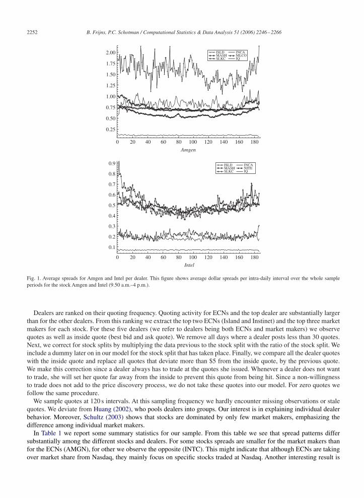
Fig. 1. Average spreads for Amgen and Intel per dealer. This figure shows average dollar spreads per intra-daily interval over the whole sampleperiods for the stock Amgen and Intel (9.50 a.m.–4 p.m.).
Dealers are ranked on their quoting frequency. Quoting activity for ECNs and the top dealer are substantially largerthan for the other dealers. From this ranking we extract the top two ECNs (Island and Instinet) and the top three marketmakers for each stock. For these five dealers (we refer to dealers being both ECNs and market makers) we observequotes as well as inside quote (best bid and ask quote). We remove all days where a dealer posts less than 30 quotes.Next, we correct for stock splits by multiplying the data previous to the stock split with the ratio of the stock split. Weinclude a dummy later on in our model for the stock split that has taken place. Finally, we compare all the dealer quoteswith the inside quote and replace all quotes that deviate more than $5 from the inside quote, by the previous quote.We make this correction since a dealer always has to trade at the quotes she issued. Whenever a dealer does not wantto trade, she will set her quote far away from the inside to prevent this quote from being hit. Since a non-willingnessto trade does not add to the price discovery process, we do not take these quotes into our model. For zero quotes wefollow the same procedure.
We sample quotes at 120 s intervals. At this sampling frequency we hardly encounter missing observations or stalequotes. We deviate from Huang (2002), who pools dealers into groups. Our interest is in explaining individual dealerbehavior. Moreover, Schultz (2003) shows that stocks are dominated by only few market makers, emphasizing thedifference among individual market makers.
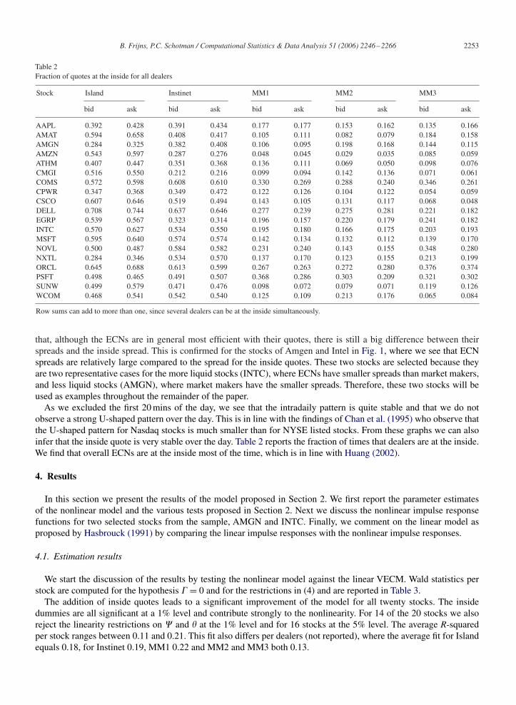
In Table 1 we report some summary statistics for our sample. From this table we see that spread patterns differsubstantially among the different stocks and dealers. For some stocks spreads are smaller for the market makers thanfor the ECNs (AMGN), for other we observe the opposite (INTC). This might indicate that although ECNs are takingover market share from Nasdaq, they mainly focus on specific stocks traded at Nasdaq. Another interesting result is
B. Frijns, P.C. Schotman / Computational Statistics & Data Analysis 51 (2006) 2246–2266 2253
Table 2Fraction of quotes at the inside for all dealers
Stock Island Instinet MM1 MM2 MM3
bid ask bid ask bid ask bid ask bid ask
AAPL 0.392 0.428 0.391 0.434 0.177 0.177 0.153 0.162 0.135 0.166AMAT 0.594 0.658 0.408 0.417 0.105 0.111 0.082 0.079 0.184 0.158AMGN 0.284 0.325 0.382 0.408 0.106 0.095 0.198 0.168 0.144 0.115AMZN 0.543 0.597 0.287 0.276 0.048 0.045 0.029 0.035 0.085 0.059ATHM 0.407 0.447 0.351 0.368 0.136 0.111 0.069 0.050 0.098 0.076CMGI 0.516 0.550 0.212 0.216 0.099 0.094 0.142 0.136 0.071 0.061COMS 0.572 0.598 0.608 0.610 0.330 0.269 0.288 0.240 0.346 0.261CPWR 0.347 0.368 0.349 0.472 0.122 0.126 0.104 0.122 0.054 0.059CSCO 0.607 0.646 0.519 0.494 0.143 0.105 0.131 0.117 0.068 0.048DELL 0.708 0.744 0.637 0.646 0.277 0.239 0.275 0.281 0.221 0.182EGRP 0.539 0.567 0.323 0.314 0.196 0.157 0.220 0.179 0.241 0.182INTC 0.570 0.627 0.534 0.550 0.195 0.180 0.166 0.175 0.203 0.193MSFT 0.595 0.640 0.574 0.574 0.142 0.134 0.132 0.112 0.139 0.170NOVL 0.500 0.487 0.584 0.582 0.231 0.240 0.143 0.155 0.348 0.280NXTL 0.284 0.346 0.534 0.570 0.137 0.170 0.123 0.155 0.213 0.199ORCL 0.645 0.688 0.613 0.599 0.267 0.263 0.272 0.280 0.376 0.374PSFT 0.498 0.465 0.491 0.507 0.368 0.286 0.303 0.209 0.321 0.302SUNW 0.499 0.579 0.471 0.476 0.098 0.072 0.079 0.071 0.119 0.126WCOM 0.468 0.541 0.542 0.540 0.125 0.109 0.213 0.176 0.065 0.084
Row sums can add to more than one, since several dealers can be at the inside simultaneously.
that, although the ECNs are in general most efficient with their quotes, there is still a big difference between theirspreads and the inside spread. This is confirmed for the stocks of Amgen and Intel in Fig. 1, where we see that ECNspreads are relatively large compared to the spread for the inside quotes. These two stocks are selected because theyare two representative cases for the more liquid stocks (INTC), where ECNs have smaller spreads than market makers,and less liquid stocks (AMGN), where market makers have the smaller spreads. Therefore, these two stocks will beused as examples throughout the remainder of the paper.
As we excluded the first 20 mins of the day, we see that the intradaily pattern is quite stable and that we do notobserve a strong U-shaped pattern over the day. This is in line with the findings of Chan et al. (1995) who observe thatthe U-shaped pattern for Nasdaq stocks is much smaller than for NYSE listed stocks. From these graphs we can alsoinfer that the inside quote is very stable over the day. Table 2 reports the fraction of times that dealers are at the inside.We find that overall ECNs are at the inside most of the time, which is in line with Huang (2002).
4. Results
In this section we present the results of the model proposed in Section 2. We first report the parameter estimatesof the nonlinear model and the various tests proposed in Section 2. Next we discuss the nonlinear impulse responsefunctions for two selected stocks from the sample, AMGN and INTC. Finally, we comment on the linear model asproposed by Hasbrouck (1991) by comparing the linear impulse responses with the nonlinear impulse responses.
4.1. Estimation results
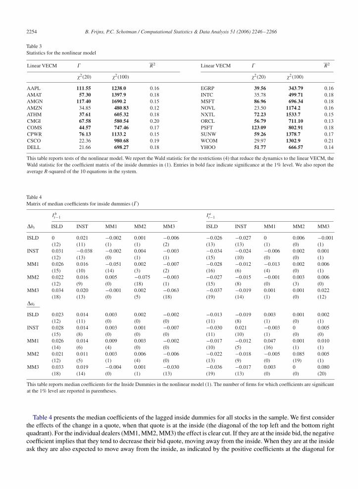
We start the discussion of the results by testing the nonlinear model against the linear VECM. Wald statistics perstock are computed for the hypothesis � = 0 and for the restrictions in (4) and are reported in Table 3.
The addition of inside quotes leads to a significant improvement of the model for all twenty stocks. The insidedummies are all significant at a 1% level and contribute strongly to the nonlinearity. For 14 of the 20 stocks we alsoreject the linearity restrictions on � and � at the 1% level and for 16 stocks at the 5% level. The average R-squaredper stock ranges between 0.11 and 0.21. This fit also differs per dealers (not reported), where the average fit for Islandequals 0.18, for Instinet 0.19, MM1 0.22 and MM2 and MM3 both 0.13.
2254 B. Frijns, P.C. Schotman / Computational Statistics & Data Analysis 51 (2006) 2246–2266
Table 3Statistics for the nonlinear model
Linear VECM � R2 Linear VECM � R2
2(20) 2(100) 2(20) 2(100)
AAPL 111.55 1238.0 0.16 EGRP 39.56 343.79 0.16AMAT 57.30 1397.9 0.18 INTC 35.78 499.71 0.18AMGN 117.40 1690.2 0.15 MSFT 86.96 696.34 0.18AMZN 34.85 480.83 0.12 NOVL 23.50 1174.2 0.16ATHM 37.61 605.32 0.18 NXTL 72.23 1533.7 0.15CMGI 67.58 580.54 0.20 ORCL 56.79 711.10 0.13COMS 44.57 747.46 0.17 PSFT 123.09 802.91 0.18CPWR 76.13 1133.2 0.15 SUNW 59.26 1378.7 0.17CSCO 22.36 980.68 0.19 WCOM 29.97 1302.9 0.21DELL 21.66 698.27 0.18 YHOO 51.77 666.57 0.14
This table reports tests of the nonlinear model. We report the Wald statistic for the restrictions (4) that reduce the dynamics to the linear VECM, theWald statistic for the coefficient matrix of the inside dummies in (1). Entries in bold face indicate significance at the 1% level. We also report theaverage R-squared of the 10 equations in the system.
Table 4Matrix of median coefficients for inside dummies (�)
I bt−1 I a
t−1
�bt ISLD INST MM1 MM2 MM3 ISLD INST MM1 MM2 MM3
ISLD 0 0.021 −0.002 0.001 −0.006 −0.026 −0.027 0 0.006 −0.001(12) (11) (1) (1) (2) (13) (13) (1) (0) (1)
INST 0.031 −0.038 −0.002 0.004 −0.003 −0.034 −0.024 −0.006 0.002 0.001(12) (13) (0) (1) (1) (15) (10) (0) (0) (1)
MM1 0.026 0.016 −0.051 0.002 −0.007 −0.028 −0.012 −0.013 0.002 0.006(15) (10) (14) (3) (2) (16) (6) (4) (0) (1)
MM2 0.022 0.016 0.005 −0.075 −0.003 −0.027 −0.015 −0.001 0.003 0.006(12) (9) (0) (18) (1) (15) (8) (0) (3) (0)
MM3 0.034 0.020 −0.001 0.002 −0.063 −0.037 −0.019 0.001 0.001 0.022(18) (13) (0) (5) (18) (19) (14) (1) (0) (12)
�at
ISLD 0.023 0.014 0.003 0.002 −0.002 −0.013 −0.019 0.003 0.001 0.002(12) (11) (0) (0) (0) (11) (8) (1) (0) (1)
INST 0.028 0.014 0.003 0.001 −0.007 −0.030 0.021 −0.003 0 0.005(15) (8) (0) (0) (0) (11) (10) (1) (0) (0)
MM1 0.026 0.014 0.009 0.003 −0.002 −0.017 −0.012 0.047 0.001 0.010(14) (6) (4) (0) (0) (10) (5) (16) (1) (1)
MM2 0.021 0.011 0.003 0.006 −0.006 −0.022 −0.018 −0.005 0.085 0.005(12) (5) (1) (4) (0) (13) (9) (0) (19) (1)
MM3 0.033 0.019 −0.004 0.001 −0.030 −0.036 −0.017 0.003 0 0.080(18) (14) (0) (1) (13) (19) (13) (0) (0) (20)
This table reports median coefficients for the Inside Dummies in the nonlinear model (1). The number of firms for which coefficients are significantat the 1% level are reported in parentheses.
Table 4 presents the median coefficients of the lagged inside dummies for all stocks in the sample. We first considerthe effects of the change in a quote, when that quote is at the inside (the diagonal of the top left and the bottom rightquadrant). For the individual dealers (MM1, MM2, MM3) the effect is clear cut. If they are at the inside bid, the negativecoefficient implies that they tend to decrease their bid quote, moving away from the inside. When they are at the insideask they are also expected to move away from the inside, as indicated by the positive coefficients at the diagonal for
B. Frijns, P.C. Schotman / Computational Statistics & Data Analysis 51 (2006) 2246–2266 2255
Table 5Matrix of median coefficients for lagged quotes (�)
�bt−1 �at−1
�bt ISLD INST MM1 MM2 MM3 ISLD INST MM1 MM2 MM3
ISLD −0.101 0.004 −0.001 −0.003 −0.001 0.038 0.013 0.001 0.010 0.015(18) (0) (0) (1) (0) (15) (2) (0) (0) (0)
INST 0.008 −0.129 0.006 0.002 0.001 0.027 0.015 0.010 0.009 0.016(1) (17) (0) (0) (0) (10) (3) (2) (1) (1)
MM1 0 0.006 −0.105 0 −0.004 0.015 0.014 0.024 0.015 0.020(1) (1) (20) (5) (2) (5) (6) (6) (2) (2)
MM2 0.010 0.012 0.008 −0.108 0.013 0.032 0.017 0.005 0.024 0.003(2) (2) (2) (19) (3) (8) (7) (1) (7) (0)
MM3 0.016 0.014 0.019 0.005 −0.097 0.028 0.016 0.011 0.006 0.019(5) (8) (6) (4) (15) (10) (7) (2) (1) (3)
�at
ISLD 0.033 0.013 0.008 0.004 0.004 −0.098 −0.004 −0.011 −0.001 −0.003(13) (4) (1) (0) (0) (15) (1) (2) (0) (0)
INST 0.022 0.016 0.015 0.011 0.014 0.007 −0.133 −0.011 −0.004 0.002(11) (2) (6) (1) (0) (3) (19) (0) (0) (1)
MM1 0.014 0.012 0.025 0.011 0.029 −0.002 0.003 −0.127 −0.008 0.002(5) (5) (8) (3) (7) (1) (1) (20) (2) (2)
MM2 0.020 0.018 0.015 0.018 0.021 0.010 0.003 −0.005 −0.116 −0.004(9) (8) (5) (5) (3) (4) (2) (1) (19) (1)
MM3 0.018 0.015 0.019 0.007 0.027 0.023 0.011 −0.002 0.005 −0.096(8) (6) (7) (4) (6) (6) (4) (2) (2) (17)
This table reports median coefficients for the lagged quotes (�) in the nonlinear model (1). The number of firms for which coefficients are significantat the 1% level are reported in parentheses.
the ask dynamics. The estimates are significant for most stocks at the 1% level. The results are different for the twoECNs. Here the coefficients are less often significant and the median over all stocks is much closer to zero. The effectsare particularly small to non-existent for Island.
There are several interesting cross-effects observed in the table. First, there is a positive and symmetric reaction ofother dealers’ bid and ask quotes (the first columns of each quadrant) to Island being at the inside bid. Dealers tend toraise both quotes with the same amount when Island is at the inside bid. A similar result is obtained when Island is atthe inside ask, all other dealers tend to lower their quotes, again in a symmetric fashion. This is an indication of theimportance of this ECN. For Instinet the results are similar, though less significant. On the other side of the spectrumwe observe the reaction of the ECNs to market makers being at the inside. There is only a very small reaction of ECNsto market makers being at the inside, with only few significant coefficients.
In Table 5 we present the median coefficients of the AR(1) component. All coefficients along the main diagonal arenegative. Hence, when a dealer raises a quote she is more inclined to lower that quote again in the next period. Themagnitude of this effect is the same for all dealers. Furthermore, there are some cross effects present between the bidand ask of the same dealer, but most of the other cross effects are insignificant.
Table 6 presents the median coefficients of the error correction term. Again we observe a strong effect along themain diagonal, where all coefficients are negative and significant. Hence, all dealers adjust their quotes towardsthe respective inside quotes. Note that these coefficients get smaller in absolute terms for the less active dealers.This is in line with the fractions of time a dealer is at the inside as we observed in Table 2 and indicates that er-ror correction effects are stronger for ECNs than for market makers. We hardly observe cross effects between bidand ask quotes of the same dealer, except for market maker 3, who has her other quote moving away from theinside (market maker 3 is often represented by the same market maker SLKC). This indicates that dealers only fo-cus on the respective inside quote and do not consider the other inside quote. All other cross effects are mostlyinsignificant.
2256 B. Frijns, P.C. Schotman / Computational Statistics & Data Analysis 51 (2006) 2246–2266
Table 6Matrix of median coefficients for error correction term (�)
(bt−1 − �iqbt−1) (at−1 − �iqa
t−1)
�bt ISLD INST MM1 MM2 MM3 ISLD INST MM1 MM2 MM3
ISLD −0.604 0.021 0.031 0.014 0.011 −0.010 0.013 0.010 0.003 −0.005(20) (9) (11) (5) (4) (5) (1) (3) (0) (2)
INST 0.024 −0.530 0.019 0.012 0.018 0.006 0.002 0 −0.004 −0.016(3) (20) (2) (6) (5) (1) (4) (2) (0) (2)
MM1 0.033 0.028 −0.553 0.023 0.017 0.009 0.003 −0.021 −0.004 −0.011(12) (7) (20) (13) (9) (3) (3) (6) (2) (3)
MM2 0.018 0.011 0.012 −0.241 0.010 0.003 0.004 −0.004 −0.021 −0.006(5) (4) (2) (19) (3) (0) (1) (4) (9) (3)
MM3 0.021 0.010 0 −0.002 −0.215 0.009 0.005 −0.009 −0.002 −0.086(3) (3) (5) (4) (20) (2) (1) (5) (0) (16)
�at
ISLD −0.006 0.009 0.006 0.001 −0.002 −0.630 0.034 0.047 0.024 0.018(5) (2) (1) (3) (3) (20) (9) (17) (10) (4)
INST −0.004 0.007 −0.006 −0.001 −0.013 0.036 −0.486 0.045 0.017 0.021(1) (2) (0) (1) (3) (8) (20) (14) (9) (8)
MM1 0.002 0.002 −0.030 0 −0.024 0.069 0.040 −0.435 0.030 0.030(2) (0) (8) (6) (11) (19) (15) (20) (16) (11)
MM2 0.005 0 −0.012 −0.023 −0.008 0.025 0.015 0.024 −0.208 0.013(1) (0) (4) (11) (5) (8) (6) (9) (20) (7)
MM3 0.003 0.002 −0.009 −0.003 −0.079 0.012 0.016 0.009 0.007 −0.199(1) (1) (1) (3) (18) (3) (6) (7) (6) (20)
This table reports median coefficients for the error correction term (�) in the nonlinear model (1). The number of firms for which coefficients aresignificant at the 1% level are reported in parentheses.
Table 7Median coefficients for the inside spread (�)
�bt aiqt−1 − biqt−1 �at aiqt−1 − biqt−1
ISLD 0.305 (17) ISLD −0.135 (10)INST 0.340 (19) INST −0.164 (12)MM1 0.205 (17) MM1 −0.066 (5)MM2 0.170 (13) MM2 −0.026 (2)MM3 0.121 (7) MM3 −0.004 (5)
This table reports results for inside spread coefficients in model (1). We report median coefficients for � and the number of firms for which � issignificant at the 1% level.
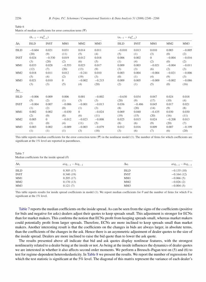
Table 7 reports the median coefficients on the inside spread. As can be seen from the signs of the coefficients (positivefor bids and negative for asks) dealers adjust their quotes to keep spreads small. This adjustment is stronger for ECNsthan for market makers. This confirms the notion that ECNs profit from keeping spreads small, whereas market makerscould potentially profit from larger spreads. Therefore, ECNs are more inclined to keep spreads small than marketmakers. Another interesting result is that the coefficients on the changes in bids are always larger, in absolute terms,than the coefficients of the changes in the ask. Hence there is an asymmetric adjustment of dealer quotes to the size ofthe inside spread. Dealers are more inclined to raise the bid quote than to lower the ask quote.
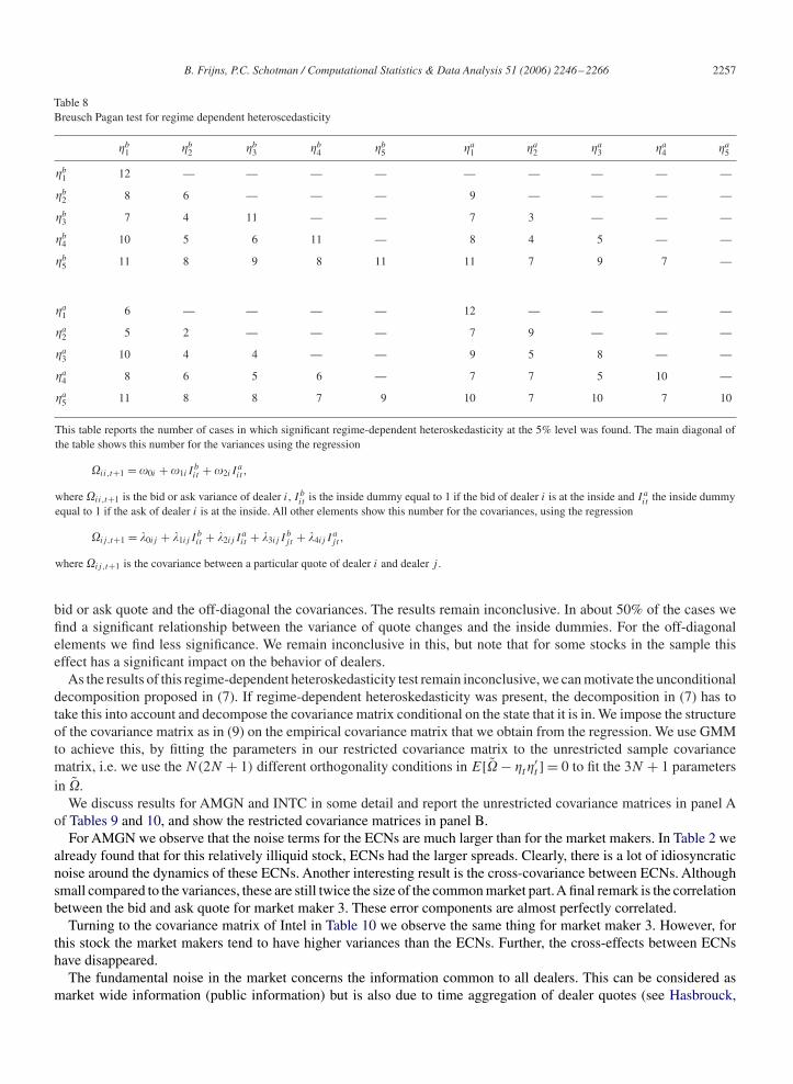
The results presented above all indicate that bid and ask quotes display nonlinear features, with the strongestnonlinearity related to a dealer being at the inside or not. As being at the inside influences the dynamics of dealer quoteswe are interested in whether it also affects second order moments. We perform a Breusch–Pagan test on (5) and (6) totest for regime-dependent heteroskedasticity. In Table 8 we present the results. We report the number of regressions forwhich the test statistic is significant at the 5% level. The diagonal of this matrix represent the variance of each dealer’s
B. Frijns, P.C. Schotman / Computational Statistics & Data Analysis 51 (2006) 2246–2266 2257
Table 8Breusch Pagan test for regime dependent heteroscedasticity
�b1 �b
2 �b3 �b
4 �b5 �a
1 �a2 �a
3 �a4 �a
5
�b1 12 — — — — — — — — —
�b2 8 6 — — — 9 — — — —
�b3 7 4 11 — — 7 3 — — —
�b4 10 5 6 11 — 8 4 5 — —
�b5 11 8 9 8 11 11 7 9 7 —
�a1 6 — — — — 12 — — — —
�a2 5 2 — — — 7 9 — — —
�a3 10 4 4 — — 9 5 8 — —
�a4 8 6 5 6 — 7 7 5 10 —
�a5 11 8 8 7 9 10 7 10 7 10
This table reports the number of cases in which significant regime-dependent heteroskedasticity at the 5% level was found. The main diagonal ofthe table shows this number for the variances using the regression
ii,t+1 = �0i + �1i Ibit + �2i I
ait ,
where ii,t+1 is the bid or ask variance of dealer i, I bit is the inside dummy equal to 1 if the bid of dealer i is at the inside and I a
it the inside dummyequal to 1 if the ask of dealer i is at the inside. All other elements show this number for the covariances, using the regression
ij ,t+1 = �0ij + �1ij Ibit + �2ij I
ait + �3ij I
bj t + �4ij I
aj t ,
where ij ,t+1 is the covariance between a particular quote of dealer i and dealer j .
bid or ask quote and the off-diagonal the covariances. The results remain inconclusive. In about 50% of the cases wefind a significant relationship between the variance of quote changes and the inside dummies. For the off-diagonalelements we find less significance. We remain inconclusive in this, but note that for some stocks in the sample thiseffect has a significant impact on the behavior of dealers.
As the results of this regime-dependent heteroskedasticity test remain inconclusive, we can motivate the unconditionaldecomposition proposed in (7). If regime-dependent heteroskedasticity was present, the decomposition in (7) has totake this into account and decompose the covariance matrix conditional on the state that it is in. We impose the structureof the covariance matrix as in (9) on the empirical covariance matrix that we obtain from the regression. We use GMMto achieve this, by fitting the parameters in our restricted covariance matrix to the unrestricted sample covariancematrix, i.e. we use the N(2N + 1) different orthogonality conditions in E[ − �t�
′t ] = 0 to fit the 3N + 1 parameters
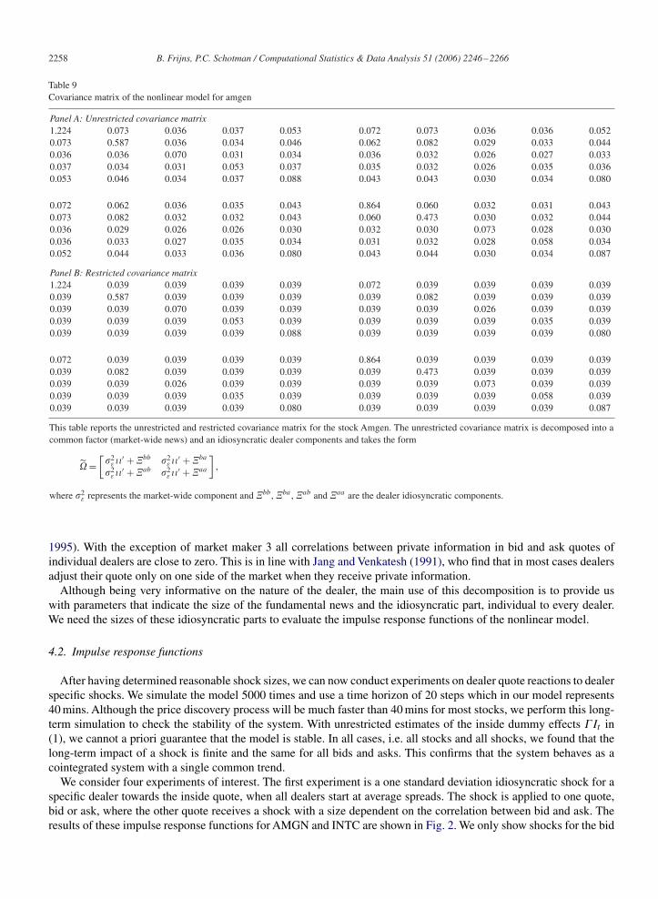
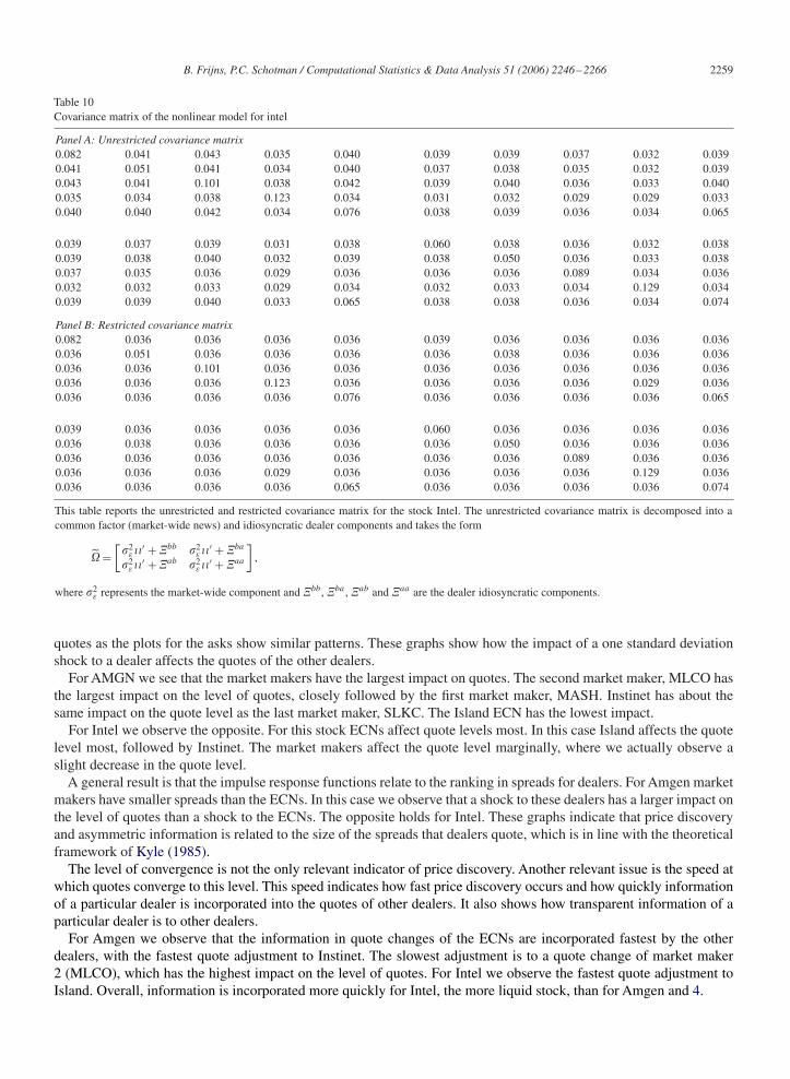
in .We discuss results for AMGN and INTC in some detail and report the unrestricted covariance matrices in panel A
of Tables 9 and 10, and show the restricted covariance matrices in panel B.For AMGN we observe that the noise terms for the ECNs are much larger than for the market makers. In Table 2 we
already found that for this relatively illiquid stock, ECNs had the larger spreads. Clearly, there is a lot of idiosyncraticnoise around the dynamics of these ECNs. Another interesting result is the cross-covariance between ECNs. Althoughsmall compared to the variances, these are still twice the size of the common market part.A final remark is the correlationbetween the bid and ask quote for market maker 3. These error components are almost perfectly correlated.
Turning to the covariance matrix of Intel in Table 10 we observe the same thing for market maker 3. However, forthis stock the market makers tend to have higher variances than the ECNs. Further, the cross-effects between ECNshave disappeared.
The fundamental noise in the market concerns the information common to all dealers. This can be considered asmarket wide information (public information) but is also due to time aggregation of dealer quotes (see Hasbrouck,
2258 B. Frijns, P.C. Schotman / Computational Statistics & Data Analysis 51 (2006) 2246–2266
Table 9Covariance matrix of the nonlinear model for amgen
Panel A: Unrestricted covariance matrix1.224 0.073 0.036 0.037 0.053 0.072 0.073 0.036 0.036 0.0520.073 0.587 0.036 0.034 0.046 0.062 0.082 0.029 0.033 0.0440.036 0.036 0.070 0.031 0.034 0.036 0.032 0.026 0.027 0.0330.037 0.034 0.031 0.053 0.037 0.035 0.032 0.026 0.035 0.0360.053 0.046 0.034 0.037 0.088 0.043 0.043 0.030 0.034 0.080
0.072 0.062 0.036 0.035 0.043 0.864 0.060 0.032 0.031 0.0430.073 0.082 0.032 0.032 0.043 0.060 0.473 0.030 0.032 0.0440.036 0.029 0.026 0.026 0.030 0.032 0.030 0.073 0.028 0.0300.036 0.033 0.027 0.035 0.034 0.031 0.032 0.028 0.058 0.0340.052 0.044 0.033 0.036 0.080 0.043 0.044 0.030 0.034 0.087
Panel B: Restricted covariance matrix1.224 0.039 0.039 0.039 0.039 0.072 0.039 0.039 0.039 0.0390.039 0.587 0.039 0.039 0.039 0.039 0.082 0.039 0.039 0.0390.039 0.039 0.070 0.039 0.039 0.039 0.039 0.026 0.039 0.0390.039 0.039 0.039 0.053 0.039 0.039 0.039 0.039 0.035 0.0390.039 0.039 0.039 0.039 0.088 0.039 0.039 0.039 0.039 0.080
0.072 0.039 0.039 0.039 0.039 0.864 0.039 0.039 0.039 0.0390.039 0.082 0.039 0.039 0.039 0.039 0.473 0.039 0.039 0.0390.039 0.039 0.026 0.039 0.039 0.039 0.039 0.073 0.039 0.0390.039 0.039 0.039 0.035 0.039 0.039 0.039 0.039 0.058 0.0390.039 0.039 0.039 0.039 0.080 0.039 0.039 0.039 0.039 0.087
This table reports the unrestricted and restricted covariance matrix for the stock Amgen. The unrestricted covariance matrix is decomposed into acommon factor (market-wide news) and an idiosyncratic dealer components and takes the form
=[�2
ε��′ + �bb �2
ε��′ + �ba
�2�
′ + �ab �2ε��
′ + �aa
],
where �2ε represents the market-wide component and �bb , �ba , �ab and �aa are the dealer idiosyncratic components.
1995). With the exception of market maker 3 all correlations between private information in bid and ask quotes ofindividual dealers are close to zero. This is in line with Jang and Venkatesh (1991), who find that in most cases dealersadjust their quote only on one side of the market when they receive private information.
Although being very informative on the nature of the dealer, the main use of this decomposition is to provide uswith parameters that indicate the size of the fundamental news and the idiosyncratic part, individual to every dealer.We need the sizes of these idiosyncratic parts to evaluate the impulse response functions of the nonlinear model.
4.2. Impulse response functions
After having determined reasonable shock sizes, we can now conduct experiments on dealer quote reactions to dealerspecific shocks. We simulate the model 5000 times and use a time horizon of 20 steps which in our model represents40 mins. Although the price discovery process will be much faster than 40 mins for most stocks, we perform this long-term simulation to check the stability of the system. With unrestricted estimates of the inside dummy effects �It in(1), we cannot a priori guarantee that the model is stable. In all cases, i.e. all stocks and all shocks, we found that thelong-term impact of a shock is finite and the same for all bids and asks. This confirms that the system behaves as acointegrated system with a single common trend.
We consider four experiments of interest. The first experiment is a one standard deviation idiosyncratic shock for aspecific dealer towards the inside quote, when all dealers start at average spreads. The shock is applied to one quote,bid or ask, where the other quote receives a shock with a size dependent on the correlation between bid and ask. Theresults of these impulse response functions for AMGN and INTC are shown in Fig. 2. We only show shocks for the bid
B. Frijns, P.C. Schotman / Computational Statistics & Data Analysis 51 (2006) 2246–2266 2259
Table 10Covariance matrix of the nonlinear model for intel
Panel A: Unrestricted covariance matrix0.082 0.041 0.043 0.035 0.040 0.039 0.039 0.037 0.032 0.0390.041 0.051 0.041 0.034 0.040 0.037 0.038 0.035 0.032 0.0390.043 0.041 0.101 0.038 0.042 0.039 0.040 0.036 0.033 0.0400.035 0.034 0.038 0.123 0.034 0.031 0.032 0.029 0.029 0.0330.040 0.040 0.042 0.034 0.076 0.038 0.039 0.036 0.034 0.065
0.039 0.037 0.039 0.031 0.038 0.060 0.038 0.036 0.032 0.0380.039 0.038 0.040 0.032 0.039 0.038 0.050 0.036 0.033 0.0380.037 0.035 0.036 0.029 0.036 0.036 0.036 0.089 0.034 0.0360.032 0.032 0.033 0.029 0.034 0.032 0.033 0.034 0.129 0.0340.039 0.039 0.040 0.033 0.065 0.038 0.038 0.036 0.034 0.074
Panel B: Restricted covariance matrix0.082 0.036 0.036 0.036 0.036 0.039 0.036 0.036 0.036 0.0360.036 0.051 0.036 0.036 0.036 0.036 0.038 0.036 0.036 0.0360.036 0.036 0.101 0.036 0.036 0.036 0.036 0.036 0.036 0.0360.036 0.036 0.036 0.123 0.036 0.036 0.036 0.036 0.029 0.0360.036 0.036 0.036 0.036 0.076 0.036 0.036 0.036 0.036 0.065
0.039 0.036 0.036 0.036 0.036 0.060 0.036 0.036 0.036 0.0360.036 0.038 0.036 0.036 0.036 0.036 0.050 0.036 0.036 0.0360.036 0.036 0.036 0.036 0.036 0.036 0.036 0.089 0.036 0.0360.036 0.036 0.036 0.029 0.036 0.036 0.036 0.036 0.129 0.0360.036 0.036 0.036 0.036 0.065 0.036 0.036 0.036 0.036 0.074
This table reports the unrestricted and restricted covariance matrix for the stock Intel. The unrestricted covariance matrix is decomposed into acommon factor (market-wide news) and idiosyncratic dealer components and takes the form
=[�2
ε��′ + �bb �2
ε��′ + �ba
�2�
′ + �ab �2ε��
′ + �aa
],
where �2ε represents the market-wide component and �bb , �ba , �ab and �aa are the dealer idiosyncratic components.
quotes as the plots for the asks show similar patterns. These graphs show how the impact of a one standard deviationshock to a dealer affects the quotes of the other dealers.
For AMGN we see that the market makers have the largest impact on quotes. The second market maker, MLCO hasthe largest impact on the level of quotes, closely followed by the first market maker, MASH. Instinet has about thesame impact on the quote level as the last market maker, SLKC. The Island ECN has the lowest impact.
For Intel we observe the opposite. For this stock ECNs affect quote levels most. In this case Island affects the quotelevel most, followed by Instinet. The market makers affect the quote level marginally, where we actually observe aslight decrease in the quote level.
A general result is that the impulse response functions relate to the ranking in spreads for dealers. For Amgen marketmakers have smaller spreads than the ECNs. In this case we observe that a shock to these dealers has a larger impact onthe level of quotes than a shock to the ECNs. The opposite holds for Intel. These graphs indicate that price discoveryand asymmetric information is related to the size of the spreads that dealers quote, which is in line with the theoreticalframework of Kyle (1985).
The level of convergence is not the only relevant indicator of price discovery. Another relevant issue is the speed atwhich quotes converge to this level. This speed indicates how fast price discovery occurs and how quickly informationof a particular dealer is incorporated into the quotes of other dealers. It also shows how transparent information of aparticular dealer is to other dealers.
For Amgen we observe that the information in quote changes of the ECNs are incorporated fastest by the otherdealers, with the fastest quote adjustment to Instinet. The slowest adjustment is to a quote change of market maker2 (MLCO), which has the highest impact on the level of quotes. For Intel we observe the fastest quote adjustment toIsland. Overall, information is incorporated more quickly for Intel, the more liquid stock, than for Amgen and 4.
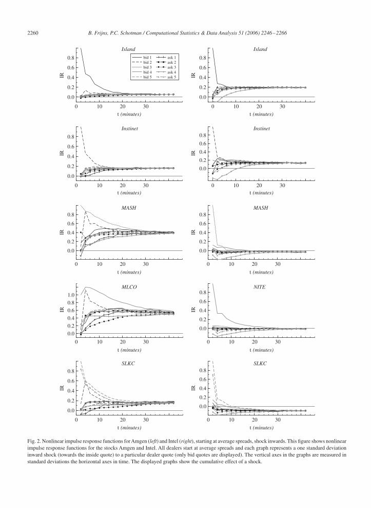
2260 B. Frijns, P.C. Schotman / Computational Statistics & Data Analysis 51 (2006) 2246–2266
0 10 20 30
0.0
0.2
0.4
0.6
0.8
Island
bid 1 bid 2 bid 3 bid 4 bid 5
ask 1 ask 2 ask 3 ask 4 ask 5
0 10 20 30
0.0
0.2
0.4
0.6
0.8
Island
0 10 20 30
0.0
0.2
0.4
0.6
0.8
Instinet
0 10 20 30
0.0
0.2
0.4
0.6
0.8Instinet
0 10 20 30
0.0
0.2
0.4
0.6
0.8MASH
0 10 20 30
0.0
0.2
0.4
0.6
0.8MASH
0 10 20 30
0.0
0.2
0.4
0.6
0.8
1.0
MLCO
0 10 20 30
0.0
0.2
0.4
0.6
0.8NITE
0 10 20 30
0.0
0.2
0.4
0.6
0.8
SLKC
0 10 20 30
0.0
0.2
0.4
0.6
0.8SLKC
IR
IRIR
IRIR
IR
IRIR
IRIR
t (minutes)
t (minutes)
t (minutes)
t (minutes)
t (minutes)
t (minutes)
t (minutes)
t (minutes)
t (minutes)
t (minutes)
Fig. 2. Nonlinear impulse response functions forAmgen (left) and Intel (right), starting at average spreads, shock inwards. This figure shows nonlinearimpulse response functions for the stocks Amgen and Intel. All dealers start at average spreads and each graph represents a one standard deviationinward shock (towards the inside quote) to a particular dealer quote (only bid quotes are displayed). The vertical axes in the graphs are measured instandard deviations the horizontal axes in time. The displayed graphs show the cumulative effect of a shock.
B. Frijns, P.C. Schotman / Computational Statistics & Data Analysis 51 (2006) 2246–2266 2261
0 10 20 30
0.0
0.2
0.4
0.6
0.8
Island
IRbid 1 bid 2 bid 3 bid 4 bid 5
ask 1 ask 2 ask 3 ask 4 ask 5
0 10 20 30
0.0
0.2
0.4
0.6
0.8
Island
IR0 10 20 30
0.0
0.2
0.4
0.6
0.8
Instinet
IR
t (minutes)
t (minutes)t (minutes)
t (minutes)
t (minutes)
t (minutes)
t (minutes)
t (minutes)
t (minutes)
t (minutes)
0 10 20 30
0.0
0.2
0.4
0.6
0.8Instinet
IR
0 10 20 30
0.0
0.2
0.4
0.6
0.8
MASH
IR
0 10 20 30
0.0
0.2
0.4
0.6
0.8
MASH
IR
0 10 20 30
0.0
0.2
0.4
0.6
0.8
1.0
MLCO
IR
0 10 20 30
0.0
0.2
0.4
0.6
0.8
NITE
IR
0 10 20 30
0.0
0.2
0.4
0.6
0.8
SLKC
IR
0 10 20 30
0.0
0.2
0.4
0.6
0.8
SLKC
IR
Fig. 3. Nonlinear impulse response functions forAmgen (left) and Intel (right), starting at inside for dealer, shock inwards. This figure shows nonlinearimpulse response functions for the stocks Amgen and Intel. All dealers start at the inside quote and each graph represents a one standard deviationinward shock to a particular dealer quote (only bid quotes are displayed). The vertical axes in the graphs are measured in standard deviations thehorizontal axes in time. The displayed graphs show the cumulative effect of a shock.
2262 B. Frijns, P.C. Schotman / Computational Statistics & Data Analysis 51 (2006) 2246–2266
0 10 20 30-1.0
-0.8
-0.6
-0.4
-0.2
Island
bid 1 bid 2 bid 3 bid 4 bid 5
ask 1 ask 2 ask 3 ask 4 ask 5
0 10 20 30-1.0
-0.8
-0.6
-0.4
-0.2
Island
0 10 20 30-1.0
-0.8
-0.6
-0.4
-0.2
Instinet
IR
IRIR
IRIR
IR
IRIR
IRIR
t (minutes)
t (minutes)
t (minutes)
t (minutes)
t (minutes)
t (minutes)
t (minutes)
t (minutes)
t (minutes)
t (minutes)0 10 20 30
-1.0
-0.8
-0.6
-0.4
-0.2
0.0
Instinet
0 10 20 30-1.0
-0.8
-0.6
-0.4
-0.2
MASH
0 10 20 30-1.0
-0.8
-0.6
-0.4
-0.2
0.0
MASH
0 10 20 30
-1.2-1.0-0.8-0.6-0.4-0.20.0
MLCO
0 10 20 30-1.0
-0.8
-0.6
-0.4
-0.2
0.0
NITE
0 10 20 301.0
-0.8
-0.6
-0.4
-0.2
0.0SLKC
0 10 20 30-1.0
-0.8
-0.6
-0.4
-0.2
0.0
SLKC
Fig. 4. Nonlinear impulse response functions for Amgen (left) and Intel (right), starting at inside for dealer, shock outwards. This figure showsnonlinear impulse response functions for the stocks Amgen and Intel. All dealers start at the inside and each graph represents a one standard deviationoutward shock (away from the inside) to a particular dealer quote (only bid quotes are displayed). The vertical axes in the graphs are measured instandard deviations the horizontal axes in time. The displayed graphs show the cumulative effect of a shock.
B. Frijns, P.C. Schotman / Computational Statistics & Data Analysis 51 (2006) 2246–2266 2263
0 10 20 30
0.0
0.2
0.4
0.6
0.8
Island
bid 1 bid 2 bid 3 bid 4 bid 5
ask 1 ask 2 ask 3 ask 4 ask 5
0 10 20 30
- 0.2
0.0
0.2
0.4
0.6
0.8Island
0 10 20 30
0.0
0.2
0.4
0.6
0.8
Instinet
0 10 20 30
- 0.4- 0.2
0.00.20.40.60.8
Instinet
0 10 20 30
0.0
0.2
0.4
0.6
0.8
MASH
0 10 20 30
- 0.2
0.0
0.2
0.4
0.6
0.8MASH
0 10 20 30
0.0
0.2
0.4
0.6
0.8
MLCO
0 10 20 30- 0.2
0.0
0.2
0.4
0.6
0.8
NITE
0 10 20 30
0.0
0.2
0.4
0.6
0.8
SLKC
0 10 20 30- 0.2
0.0
0.2
0.4
0.6
0.8
SLKC
IR
IRIR
IRIR
IR
IRIR
IRIR
t (minutes)
t (minutes)
t (minutes)
t (minutes)
t (minutes)
t (minutes)
t (minutes)
t (minutes)
t (minutes)
t (minutes)
Fig. 5. Nonlinear impulse response functions for Amgen (left) and Intel (right), starting at average spreads, shock reaching inside. This figure showsnonlinear impulse response functions for the stocks Amgen and Intel. All dealers start at average spreads and each graph represents an inward shockreaching the inside to a particular dealer quote (only bid quotes are displayed). The vertical axes in the graphs are measured in standard deviationsthe horizontal axes in time. The displayed graphs show the cumulative effect of a shock.
2264 B. Frijns, P.C. Schotman / Computational Statistics & Data Analysis 51 (2006) 2246–2266
0.00
0.05
0.10
0.15
0.20
0.25
0.30
0.35
0.40LinearNon-Linear
Amgen
-0.05
0.00
0.05
0.10
0.15
0.20
0.25
0.30LinearNon-Linear
Island Instinet
MASH MLCO
SLKCIntel
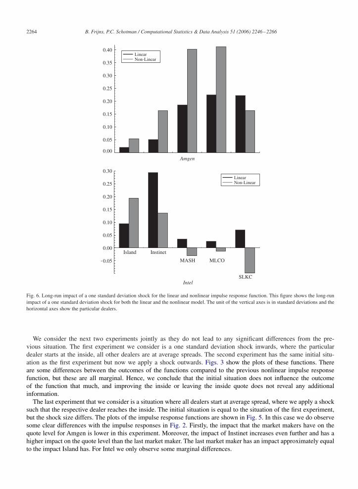
Fig. 6. Long-run impact of a one standard deviation shock for the linear and nonlinear impulse response function. This figure shows the long-runimpact of a one standard deviation shock for both the linear and the nonlinear model. The unit of the vertical axes is in standard deviations and thehorizontal axes show the particular dealers.
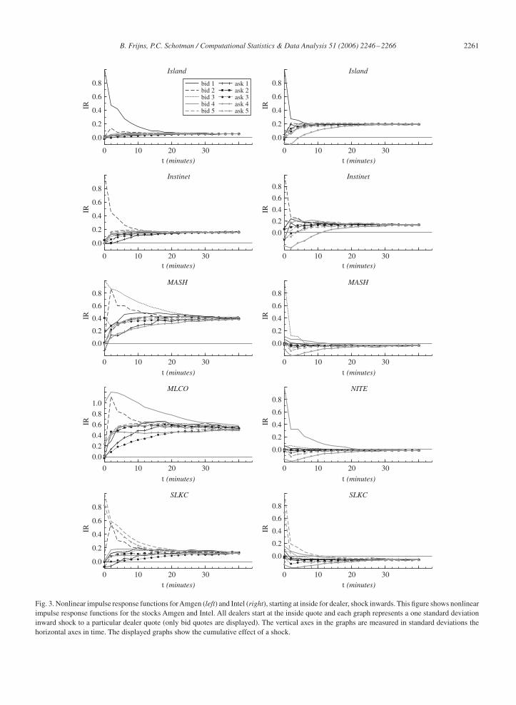
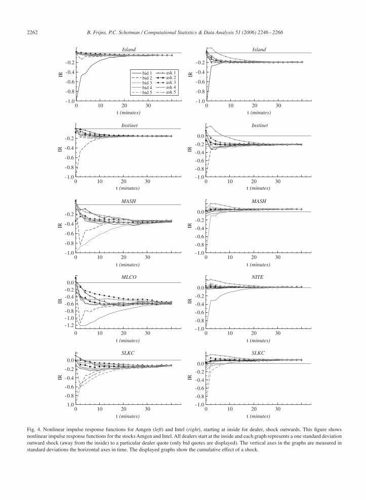
We consider the next two experiments jointly as they do not lead to any significant differences from the pre-vious situation. The first experiment we consider is a one standard deviation shock inwards, where the particulardealer starts at the inside, all other dealers are at average spreads. The second experiment has the same initial situ-ation as the first experiment but now we apply a shock outwards. Figs. 3 show the plots of these functions. Thereare some differences between the outcomes of the functions compared to the previous nonlinear impulse responsefunction, but these are all marginal. Hence, we conclude that the initial situation does not influence the outcomeof the function that much, and improving the inside or leaving the inside quote does not reveal any additionalinformation.
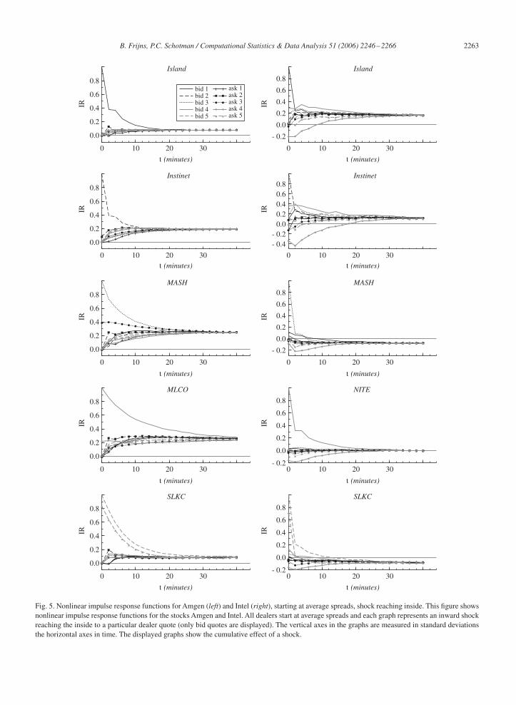
The last experiment that we consider is a situation where all dealers start at average spread, where we apply a shocksuch that the respective dealer reaches the inside. The initial situation is equal to the situation of the first experiment,but the shock size differs. The plots of the impulse response functions are shown in Fig. 5. In this case we do observesome clear differences with the impulse responses in Fig. 2. Firstly, the impact that the market makers have on thequote level for Amgen is lower in this experiment. Moreover, the impact of Instinet increases even further and has ahigher impact on the quote level than the last market maker. The last market maker has an impact approximately equalto the impact Island has. For Intel we only observe some marginal differences.
B. Frijns, P.C. Schotman / Computational Statistics & Data Analysis 51 (2006) 2246–2266 2265
Overall, the results of these responses show that the dynamics of quotes are insensitive to the initial situation, butmore sensitive to the shock size.
The question remains whether these nonlinear impulse responses lead to different results than traditional linearimpulse responses. As a robustness check we compute linear impulse responses. These are computed by estimating (1)imposing the restrictions in (3) and excluding the inside dummies. Although linear impulse responses are insensitiveto the shock size and the history of the model, we do take the correlations between a dealer’s bid and ask quote intoaccount. These are determined by the decomposition in (7).
To compare the linear impulse responses to the nonlinear impulse responses we consider the long-run impact of a onestandard deviation shock to a particular dealer for both functions. The nonlinear impulse response function consideredis a one standard deviation shock inwards, starting at average spreads (see Fig. 2). The long-run impact is determinedby the average level of bid and ask quotes of a particular dealer 40 minutes after the shock has been applied. In Fig. 6we compare the linear impulse response function to the nonlinear impulse response function for both Amgen and Intel.Since standard errors of the long-run impact coefficients are never larger than 0.04, the differences are statisticallysignificant in most cases.
ForAmgen we observe considerable differences between the linear and nonlinear specification. The largest differenceis that in the nonlinear specification shocks have a larger impact on the level of quotes. The impulse responses also leadto a different view on the importance of dealers for the price discovery process. In the linear specification market makers2 and 3 (MLCO and SLKC) appear to be the leading market makers. In the nonlinear specification the importance ofSLKC declines, whereas the importance of the other MLCO and market maker 1 (MASH) increases.
For Intel we observe an opposite pattern. In general, the impact of a one standard deviation shock on the quote leveldeclines in the nonlinear specification. Again the linear and nonlinear specification lead to different results in terms ofprice discovery. In the linear specification Instinet leads in terms of price discovery. For the nonlinear specification thisis Island.
5. Conclusion
In this paper we propose a nonlinear error correction model for quote changes, which extends the linear model ofHasbrouck (1991). Nonlinear dynamics are introduced through the inside bid and ask quotes. The model allows quoteadjustments to be different depending on who is currently at the inside and allows for an error correction towards theinside quotes instead of the midpoint. We test for a third form of nonlinearity in the distribution of the error terms,which we allow to depend on which dealer is at the inside.
Overall, we find that our model significantly improves the linear specification. Specifically, we find that all dealersstrongly correct towards the inside quotes. However, all dealers, except Island, have the tendency to move away fromthe inside when they are at the inside. We further observe that all dealer move towards the inside quote when Island ECNis at the inside. Dealers react asymmetrically to the size of the spread, by raising their bid quote more than loweringtheir ask. The results for the regime-dependent heteroskedasticity tests remain inconclusive.
Finally, we discuss price discovery in an impulse response function framework. We use a conditional bootstrap tocompute nonlinear impulse response functions. We find that the initial situation of the model does not affect the outcomeof the function, but the size of the shock does. Further, the outcomes of the nonlinear model differ substantially fromthe outcomes of the linear model. Ignoring these nonlinearities leads to different conclusions towards who dominatesin terms of price discovery.
Acknowledgments
We would like to thank Ronald Mahieu, Franz Palm, Christian Wolff and participants at the Market MicrostructureWorkshop in Madrid, March 2005, for their useful comments and suggestions.
Appendix A
Stock names and ticker symbols are reported in Table A.1.
2266 B. Frijns, P.C. Schotman / Computational Statistics & Data Analysis 51 (2006) 2246–2266
Table A.1Ticker symbols and company names
Symbol Company name Symbol Company name
AAPL Apple Computer Inc. EGRP E*TRADE Group, Inc.AMAT Applied Materials Inc. INTC Intel CorporationAMGN Amgen Inc. MSFT Microsoft CorporationAMZN Amazon.com Inc. NOVL Novell Inc.ATHM At Home Corporation NXTL Nextel CommunicationsCMGI CMGI, Inc. ORCL Oracle CorporationCOMS 3Com Corporation PSFT Peoplesoft Inc.CPWR Compuware Corporation SUNW Sun Microsystems Inc.CSCO Cisco Systems Inc. WCOM MCI WorldCom Inc.DELL Dell Computer Corporation YHOO Yahoo!, Inc.
References
Breusch, T., Pagan, A.R., 1979. A simple test for heteroskedasticity and random coefficient variation. Econometrica 47, 1287–1294.Chan, K., Christie, W.G., Schultz, P.H., 1995. Market structure and the intraday pattern of bid-ask spreads for Nasdaq securities. J. Business 68,
35–60.Christie, W.G., Schultz, P.H., 1994. Why do Nasdaq market makers avoid odd-eighth quotes? J. Finance 49, 1813–1840.Christie, W.G., Harris, J.H., Schultz, P.H., 1994. Why did Nasdaq market makers stop avoiding odd-eighth quotes? J. Finance 49, 1841–1860.Chung, K.H., Zhao, X., 2003. Intraday variation in the bid-ask spread: evidence after the market reform. J. Finan. Res. 26, 191–206.Engle, R.F., Patton, A.J., 2004. Impacts of trades in an error-correction model of quote prices. J. Finan. Markets 7, 1–25.Eun, C., Sabherwal, S., 2003. Cross-border listings and price discovery: evidence from U.S. listed Canadian stocks. J. Finance 58, 549–576.Harris, F., McInish, T.H., Chakravarty, R.R., 1995. Bids and asks in disequilibrium market microstructure: the case of IBM. J. Banking Finance 19,
323–345.Hasbrouck, J., 1991. Measuring the information content of stock trades. J. Finance 46, 179–207.Hasbrouck, J., 1995. One security, many markets: determining the contribution to price discovery. J. Finance 50, 1175–1199.Hasbrouck, J., 1999. The dynamics of discrete bid and ask quotes. J. Finance 54, 2109–2142.Huang, R.D., 2002. The quality of ECN and Nasdaq market maker quotes. J. Finance 57, 1285–1319.Jang, H., Venkatesh, P., 1991. Consistency between predicted and actual bid-ask quote revisions. J. Finance 46, 433–446.Koop, G., Pesaran, M.H., Potter, S.M., 1996. Impulse response analysis in nonlinear multivariate models. J. Econometrics 74, 119–147.Kyle, A.S., 1985. Continuous auctions and insider trading. Econometrica 53, 1315–1335.Peiers, B., 1997. Informed traders, intervention, and price leadership: a deeper view of the microstructure of the foreign exchange market. J. Finance
52, 1589–1613.Schultz, P.H., 2003. Who makes markets. J. Finan. Markets 6, 49–72.Stoll, H.R., 1989. Inferring the components of the bid-ask spread: theory and empirical tests. J. Finance 44, 115–134.Wang, J.-X., 2001. Quote revision and information flow among foreign exchange dealers. J. Int. Finan. Markets, Institutions and Money 11,
115–136.


![新ファンドのお知らせ【iFreeNEXT NASDAQ 次世代50】...2020/12/29 · [Rtf —77)' F] NASDAQ Q-50 (È) I I 12 Daiwa Asset Press Release NASDAQ Nasdaq, Inc. Nasdaq, Inc](https://img.pdfslide.us/doc/110x75/60ad0a5669e6fa12ef6df966/fffcifreenext-nasdaq-50-20201229.jpg)


![Reevaluation of Programmed I/O with Write-Combining ...benl/Publications/...arbitrage trading [1]. One example is Xasax claiming 30 microseconds delay between NASDAQ quotes and trade](https://img.pdfslide.us/doc/110x75/5f5d3cf6d45b3a4bdd23f81a/reevaluation-of-programmed-io-with-write-combining-benlpublications-arbitrage.jpg)