Embed Size (px)
Citation preview

Nonlinear diffusionequations I
JUAN LUIS VAZQUEZ
Departamento de MatematicasUniversidad Autonoma de Madridand Royal Academy of Sciences
CIME Summer Course“Nonlocal and Nonlinear Diffusions and
Interactions: New Methods and Directions”Cetraro, Italia July 4, 2016
J. L. Vazquez (UAM) Nonlinear Diffusion 1 / 47

Outline
1 Theories of DiffusionDiffusionHeat equationLinear Parabolic EquationsNonlinear equations
2 Degenerate Diffusion and Free BoundariesIntroductionThe basicsGeneralities
3 Fast Diffusion EquationFast Diffusion Ranges
J. L. Vazquez (UAM) Nonlinear Diffusion 2 / 47

Outline
1 Theories of DiffusionDiffusionHeat equationLinear Parabolic EquationsNonlinear equations
2 Degenerate Diffusion and Free BoundariesIntroductionThe basicsGeneralities
3 Fast Diffusion EquationFast Diffusion Ranges
J. L. Vazquez (UAM) Nonlinear Diffusion 3 / 47

Diffusion
Populations diffuse, substances (like particles in a solvent) diffuse, heatpropagates, electrons and ions diffuse, the momentum of a viscous(Newtonian) fluid diffuses (linearly), there is diffusion in the markets, ...
• what is diffusion anyway? Is diffusion more or less random walk ?
• how to explain it with mathematics? is it pure or applied mathematics ?what would Kolmogorov say?
• How much of it can be explained with linear models, how much isessentially nonlinear?
• The stationary states of diffusion belong to an important world, ellipticequations. Elliptic equations, linear and nonlinear, have many relatives:diffusion, fluid mechanics, waves of all types, quantum mechanics, ...
The Laplacian ∆ is the King of Differential Operators.
J. L. Vazquez (UAM) Nonlinear Diffusion 4 / 47

Diffusion in Wikipedia
Diffusion. The spreading of any quantity that can be described by thediffusion equation or a random walk model (e.g. concentration, heat,momentum, ideas, price) can be called diffusion.Some of the most important examples are listed below.* Atomic diffusion* Brownian motion, for example of a single particle in a solvent* Collective diffusion, the diffusion of a large number of (possiblyinteracting) particles * Effusion of a gas through small holes.* Electron diffusion, resulting in electric current* Facilitated diffusion, present in some organisms.* Gaseous diffusion, used for isotope separation* Heat flow * Ito- diffusion * Knudsen diffusion* Momentum diffusion, ex. the diffusion of the hydrodynamic velocity field* Osmosis is the diffusion of water through a cell membrane. * Photondiffusion* Reverse diffusion * Self-diffusion * Surface diffusion
J. L. Vazquez (UAM) Nonlinear Diffusion 5 / 47

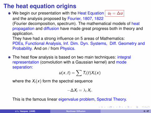
The heat equation originsWe begin our presentation with the Heat Equation ut = ∆uand the analysis proposed by Fourier, 1807, 1822(Fourier decomposition, spectrum). The mathematical models of heatpropagation and diffusion have made great progress both in theory andapplication.They have had a strong influence on 5 areas of Mathematics:PDEs, Functional Analysis, Inf. Dim. Dyn. Systems, Diff. Geometry andProbability. And on / from Physics.
The heat flow analysis is based on two main techniques: integralrepresentation (convolution with a Gaussian kernel) and modeseparation:
u(x , t) =∑
Ti (t)Xi (x)
where the Xi (x) form the spectral sequence
−∆Xi = λi Xi .
This is the famous linear eigenvalue problem, Spectral Theory.
J. L. Vazquez (UAM) Nonlinear Diffusion 6 / 47

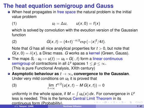
The heat equation semigroup and GaussWhen heat propagates in free space the natural problem is the initialvalue problem
(1) ut = ∆u, u(x ,0) = f (x)
which is solved by convolution with the evoution version of the Gaussianfunction
(2) G(x , t) = (4πt)−n/2exp (−|x |2/4t).
Note that G has all nice analytical properties for t > 0, but note thatG(x ,0) = δ(x), a Dirac mass. G works as a kernel (Green, Gauss).The maps St : u0 7→ u(t) := u0 ∗G(·, t) form a linear continuoussemigroup of contractions in all Lp spaces 1 ≤ p ≤ ∞.(This is pure Functional Analysis, XXth century)Asymptotic behaviour as t →∞, convergence to the Gaussian.Under very mild conditions on u0 it is proved that
(3) limt→∞
tn/2(u(x , t)−M G(x , t)) = 0
uniformly in the whole space, if M =∫
u0(x) dx . For convergence in Lp
less is needed. This is the famous Central Limit Theorem in itscontinuous form (Probability).
J. L. Vazquez (UAM) Nonlinear Diffusion 7 / 47

The personalities
J. Fourier and K. F. Gauss
J. L. Vazquez (UAM) Nonlinear Diffusion 8 / 47

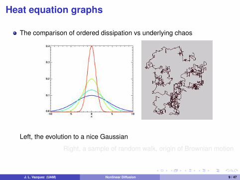
Heat equation graphs
The comparison of ordered dissipation vs underlying chaos
Left, the evolution to a nice Gaussian
Right, a sample of random walk, origin of Brownian motion
J. L. Vazquez (UAM) Nonlinear Diffusion 9 / 47

Heat equation graphs
The comparison of ordered dissipation vs underlying chaos
Left, the evolution to a nice Gaussian
Right, a sample of random walk, origin of Brownian motion
J. L. Vazquez (UAM) Nonlinear Diffusion 9 / 47
Heat equation graphs
The comparison of ordered dissipation vs underlying chaos
Left, the evolution to a nice Gaussian
Right, a sample of random walk, origin of Brownian motion
J. L. Vazquez (UAM) Nonlinear Diffusion 9 / 47

Heat equation graphs
The comparison of ordered dissipation vs underlying chaos
Left, the evolution to a nice Gaussian
Right, a sample of random walk, origin of Brownian motion
J. L. Vazquez (UAM) Nonlinear Diffusion 9 / 47

Linear heat flowsFrom 1822 until 1950 the heat equation has motivated(i) Fourier analysis decomposition of functions (and set theory),(ii) development of other linear equations=⇒ Theory of Parabolic Equations
ut =∑
aij∂i∂ju +∑
bi∂iu + cu + f
Main inventions in Parabolic Theory:(1) aij ,bi , c, f regular⇒ Maximum Principles, Schauder estimates,Harnack inequalities; Cα spaces (Holder); potential theory; generation ofsemigroups.(2) coefficients only continuous or bounded⇒W 2,p estimates,Calderon-Zygmund theory, weak solutions; Sobolev spaces.
The probabilistic approach: Diffusion as an stochastic process: Bachelier,Einstein, Smoluchowski; Kolmogorov, Wiener, Levy; Ito, Skorokhod, ...
dX = bdt + σdW
J. L. Vazquez (UAM) Nonlinear Diffusion 10 / 47
Nonlinear heat flows
In the last 50 years emphasis has shifted towards the Nonlinear World.Maths more difficult, more complex, and more realistic.My group works in the areas of Nonlinear Diffusion and ReactionDiffusion.I will talk about the theory mathematically called Nonlinear ParabolicPDEs. General formula
ut =∑∂iAi (u,∇u) +
∑B(x ,u,∇u)
Typical nonlinear diffusion: Stefan Problem, Hele-Shaw Problem, PME:ut = ∆(um), EPLE: ut = ∇ · (|∇u|p−2∇u).
Typical reaction diffusion: Fujita model ut = ∆u + up.
The fluid flow models: Navier-Stokes or Euler equation systems forincompressible flow. Any singularities?
The geometrical models: the Ricci flow, movement by curvature.
J. L. Vazquez (UAM) Nonlinear Diffusion 11 / 47

The Nonlinear Diffusion ModelsThe four classical ’sisters’ of the 1980’s
The Stefan Problem (Lame and Clapeyron, 1833; Stefan 1880)
SE :
ut = k1∆u for u > 0,ut = k2∆u for u < 0. TC :
u = 0,v = L(k1∇u1 − k2∇u2).
Main feature: the free boundary or moving boundary where u = 0. TC=Transmission conditions at u = 0.The Hele-Shaw cell (Hele-Shaw, 1898; Saffman-Taylor, 1958)
u > 0, ∆u = 0 in Ω(t); u = 0, v = L∂nu on ∂Ω(t).
The Porous Medium Equation→(hidden free boundary)
ut = ∆um, m > 1.
The p-Laplacian Equation, ut = div (|∇u|p−2∇u).
Recent interest in p = 1 (images) or p =∞ (geometry and transport)
J. L. Vazquez (UAM) Nonlinear Diffusion 12 / 47
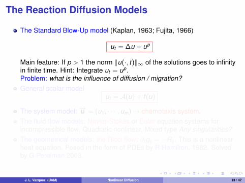
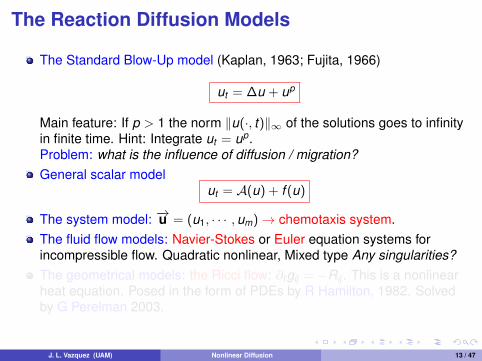
The Reaction Diffusion Models
The Standard Blow-Up model (Kaplan, 1963; Fujita, 1966)
ut = ∆u + up
Main feature: If p > 1 the norm ‖u(·, t)‖∞ of the solutions goes to infinityin finite time. Hint: Integrate ut = up.Problem: what is the influence of diffusion / migration?General scalar model
ut = A(u) + f (u)
The system model: −→u = (u1, · · · ,um)→ chemotaxis system.The fluid flow models: Navier-Stokes or Euler equation systems forincompressible flow. Quadratic nonlinear, Mixed type Any singularities?The geometrical models: the Ricci flow: ∂tgij = −Rij . This is a nonlinearheat equation. Posed in the form of PDEs by R Hamilton, 1982. Solvedby G Perelman 2003.
J. L. Vazquez (UAM) Nonlinear Diffusion 13 / 47

An opinion by John Nash, 1958:The open problems in the area of nonlinear p.d.e. are very relevant to
applied mathematics and science as a whole, perhaps more so that theopen problems in any other area of mathematics, and the field seemspoised for rapid development. It seems clear, however, that freshmethods must be employed...
Little is known about the existence, uniqueness and smoothness ofsolutions of the general equations of flow for a viscous, compressible,and heat conducting fluid...
Continuity of solutions of elliptic and parabolic equations,paper published in Amer. J. Math, 80, no 4 (1958), 931-954.
De Giorgi, Ennio, Sulla differenziabilita e l’analiticita delle estremali degliintegrali multipli regolari. Mem. Accad. Sci. Torino. Cl. Sci. Fis. Mat. Nat.(3) 3 (1957), 25–43.
J. Moser, A new proof of De Giorgi’s theorem concerning the regularityproblem for elliptic differential equations. Comm. Pure Appl. Math. 13(1960) 457–468.A Harnack inequality for parabolic differential equations, Comm. Pureand Appl. Math. 17 (1964), 101–134.
J. L. Vazquez (UAM) Nonlinear Diffusion 14 / 47

Outline
1 Theories of DiffusionDiffusionHeat equationLinear Parabolic EquationsNonlinear equations
2 Degenerate Diffusion and Free BoundariesIntroductionThe basicsGeneralities
3 Fast Diffusion EquationFast Diffusion Ranges
J. L. Vazquez (UAM) Nonlinear Diffusion 15 / 47

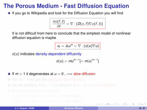
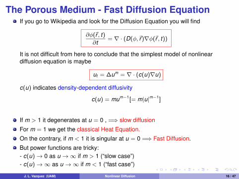
The Porous Medium - Fast Diffusion EquationIf you go to Wikipedia and look for the Diffusion Equation you will find
∂φ(~r , t)∂t
= ∇ · (D(φ,~r)∇φ(~r , t))
It is not difficult from here to conclude that the simplest model of nonlineardiffusion equation is maybe
ut = ∆um = ∇ · (c(u)∇u)
c(u) indicates density-dependent diffusivity
c(u) = mum−1[= m|u|m−1]
If m > 1 it degenerates at u = 0 , =⇒ slow diffusion
For m = 1 we get the classical Heat Equation.
On the contrary, if m < 1 it is singular at u = 0 =⇒ Fast Diffusion.
But power functions are tricky:- c(u)→ 0 as u →∞ if m > 1 (“slow case”)- c(u)→∞ as u →∞ if m < 1 (“fast case”)
J. L. Vazquez (UAM) Nonlinear Diffusion 16 / 47

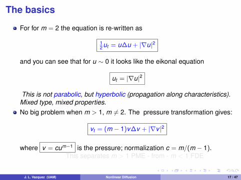
The basics
For for m = 2 the equation is re-written as
12 ut = u∆u + |∇u|2
and you can see that for u ∼ 0 it looks like the eikonal equation
ut = |∇u|2
This is not parabolic, but hyperbolic (propagation along characteristics).Mixed type, mixed properties.No big problem when m > 1, m 6= 2. The pressure transformation gives:
vt = (m − 1)v∆v + |∇v |2
where v = cum−1 is the pressure; normalization c = m/(m − 1).This separates m > 1 PME - from - m < 1 FDE
J. L. Vazquez (UAM) Nonlinear Diffusion 17 / 47

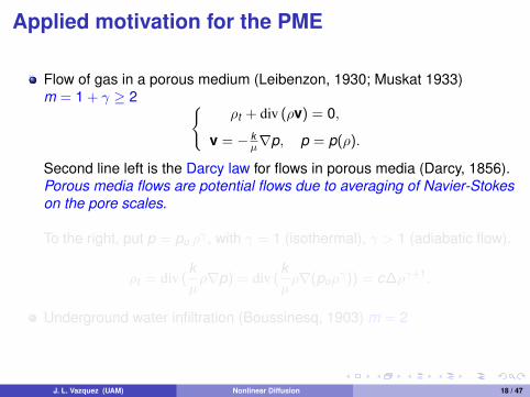
Applied motivation for the PME
Flow of gas in a porous medium (Leibenzon, 1930; Muskat 1933)m = 1 + γ ≥ 2
ρt + div (ρv) = 0,
v = − kµ∇p, p = p(ρ).
Second line left is the Darcy law for flows in porous media (Darcy, 1856).Porous media flows are potential flows due to averaging of Navier-Stokeson the pore scales.
To the right, put p = po ργ , with γ = 1 (isothermal), γ > 1 (adiabatic flow).
ρt = div (kµρ∇p) = div (
kµρ∇(poρ
γ)) = c∆ργ+1.
Underground water infiltration (Boussinesq, 1903) m = 2
J. L. Vazquez (UAM) Nonlinear Diffusion 18 / 47

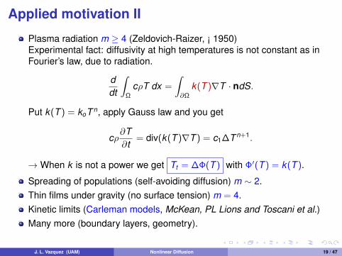
Applied motivation II
Plasma radiation m ≥ 4 (Zeldovich-Raizer, ¡ 1950)Experimental fact: diffusivity at high temperatures is not constant as inFourier’s law, due to radiation.
ddt
∫Ω
cρT dx =
∫∂Ω
k(T )∇T · ndS.
Put k(T ) = koT n, apply Gauss law and you get
cρ∂T∂t
= div(k(T )∇T ) = c1∆T n+1.
→When k is not a power we get Tt = ∆Φ(T ) with Φ′(T ) = k(T ).
Spreading of populations (self-avoiding diffusion) m ∼ 2.Thin films under gravity (no surface tension) m = 4.Kinetic limits (Carleman models, McKean, PL Lions and Toscani et al.)Many more (boundary layers, geometry).
J. L. Vazquez (UAM) Nonlinear Diffusion 19 / 47

Planning of the Theory
These are the main topics of mathematical analysis (1958-2006):The precise meaning of solution.
The nonlinear approach: estimates; functional spaces.
Existence, non-existence. Uniqueness, non-uniqueness.
Regularity of solutions: is there a limit? Ck for some k?
Regularity and movement of interfaces: Ck for some k?.
Asymptotic behaviour: patterns and rates? universal?
The probabilistic approach. Nonlinear process. Wasserstein estimates
Generalization: fast models, inhomogeneous media, anisotropic media,applications to geometry or image processing; other effects.
J. L. Vazquez (UAM) Nonlinear Diffusion 20 / 47

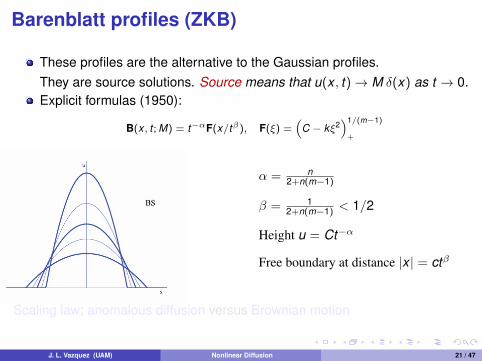
Barenblatt profiles (ZKB)
These profiles are the alternative to the Gaussian profiles.They are source solutions. Source means that u(x , t)→ M δ(x) as t → 0.Explicit formulas (1950):
B(x , t ; M) = t−αF(x/tβ), F(ξ) =(
C − kξ2)1/(m−1)
+
α = n2+n(m−1)
β = 12+n(m−1) < 1/2
Height u = Ct−α
Free boundary at distance |x | = ctβ
Scaling law; anomalous diffusion versus Brownian motion
J. L. Vazquez (UAM) Nonlinear Diffusion 21 / 47

My Russian friend
Grisha I. Barenblatt
J. L. Vazquez (UAM) Nonlinear Diffusion 22 / 47

My Russian friend
Grisha I. Barenblatt
J. L. Vazquez (UAM) Nonlinear Diffusion 22 / 47

Concept of solution
There are many concepts of generalized solution of the PME:
Classical solution: only in non-degenerate situations, u > 0.Limit solution: physical, but depends on the approximation (?).Weak solution Test against smooth functions and eliminate derivativeson the unknown function; it is the mainstream; (Oleinik, 1958)∫ ∫
(u ηt −∇um · ∇η) dxdt +
∫u0(x) η(x ,0) dx = 0.
Very weak ∫ ∫(u ηt + um ∆η) dxdt +
∫u0(x) η(x ,0) dx = 0.
J. L. Vazquez (UAM) Nonlinear Diffusion 23 / 47

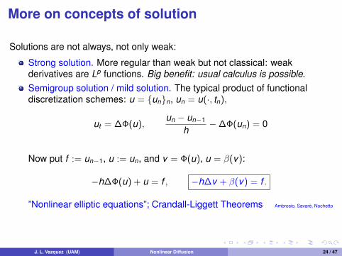
More on concepts of solution
Solutions are not always, not only weak:
Strong solution. More regular than weak but not classical: weakderivatives are Lp functions. Big benefit: usual calculus is possible.Semigroup solution / mild solution. The typical product of functionaldiscretization schemes: u = unn, un = u(·, tn),
ut = ∆Φ(u),un − un−1
h−∆Φ(un) = 0
Now put f := un−1, u := un, and v = Φ(u), u = β(v):
−h∆Φ(u) + u = f , −h∆v + β(v) = f .
”Nonlinear elliptic equations”; Crandall-Liggett Theorems Ambrosio, Savare, Nochetto
J. L. Vazquez (UAM) Nonlinear Diffusion 24 / 47

More on concepts of solution II
Solutions of more complicated diffusion-convection equations need newconcepts:
Viscosity solution Two ideas: (1) add artificial viscosity and pass to thelimit; (2) viscosity concept of Crandall-Evans-Lions (1984); adapted toPME by Caffarelli-Vazquez (1999).Entropy solution (Kruzhkov, 1968). Invented for conservation laws; itidentifies unique physical solution from spurious weak solutions. It isuseful for general models degenerate diffusion-convection models;
Renormalized solution (Di Perna - PLLions).
BV solution (Volpert-Hudjaev).
Kinetic solutions (Perthame,...).
Proper solutions (Galaktionov-Vazquez,...).
J. L. Vazquez (UAM) Nonlinear Diffusion 25 / 47

Regularity results
The universal estimate holds (Aronson-Benilan, 79):
∆v ≥ −C/t .
v ∼ um−1 is the pressure.(Caffarelli-Friedman, 1982) Cα regularity: there is an α ∈ (0,1) such thata bounded solution defined in a cube is Cα continuous.If there is an interface Γ, it is also Cα continuous in space time.How far can you go?Free boundaries are stationary (metastable) if initial profile is quadraticnear ∂Ω: u0(x) = O(d2). This is called waiting time. Characterized byJLV in 1983. Visually interesting in thin films spreading on a table.
Existence of corner points possible when metastable,⇒ no C1
Aronson-Caffarelli-V. Regularity stops here in n = 1
J. L. Vazquez (UAM) Nonlinear Diffusion 26 / 47

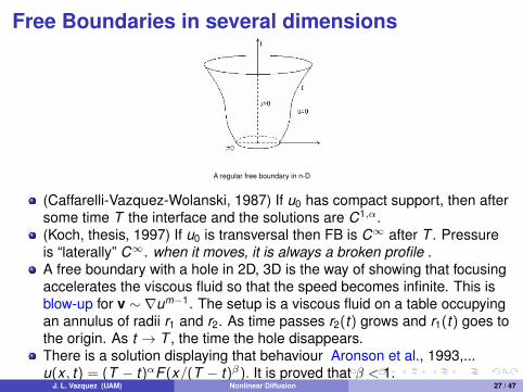
Free Boundaries in several dimensions
A regular free boundary in n-D
(Caffarelli-Vazquez-Wolanski, 1987) If u0 has compact support, then aftersome time T the interface and the solutions are C1,α.(Koch, thesis, 1997) If u0 is transversal then FB is C∞ after T . Pressureis “laterally” C∞. when it moves, it is always a broken profile .A free boundary with a hole in 2D, 3D is the way of showing that focusingaccelerates the viscous fluid so that the speed becomes infinite. This isblow-up for v ∼ ∇um−1. The setup is a viscous fluid on a table occupyingan annulus of radii r1 and r2. As time passes r2(t) grows and r1(t) goes tothe origin. As t → T , the time the hole disappears.There is a solution displaying that behaviour Aronson et al., 1993,...u(x , t) = (T − t)αF (x/(T − t)β). It is proved that β < 1.
J. L. Vazquez (UAM) Nonlinear Diffusion 27 / 47

Parabolic to EllipticSemigroup solution / mild solution. The typical product of functionaldiscretization schemes: u = unn, un = u(·, tn),
ut = ∆Φ(u),un − un−1
h−∆Φ(un) = 0
Now put f := un−1, u := un, and v = Φ(u), u = β(v):
−h∆Φ(u) + u = f , −h∆v + β(v) = f .
”Nonlinear elliptic equations”; Crandall-Liggett Theorems Ambrosio, Savare, Nochetto
Separation of variables. Put u(x , t) = F (x)G(t). Then PME gives
F (x)G′(t) = Gm(t)∆F m(x),
so that G′(t) = −Gm(t), i.e., G(t) = (m − 1)t−1/(m−1) if m > 1 and
−∆F m(x) = F (x), −∆v(x) = vp(x), p = 1/m.
This is more interesting for m < 1, specially for m = (n − 2)/(n − 2).
J. L. Vazquez (UAM) Nonlinear Diffusion 28 / 47

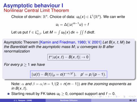
Asymptotic behaviour INonlinear Central Limit Theorem
Choice of domain: Rn. Choice of data: u0(x) ∈ L1(Rn). We can write
ut = ∆(|u|m−1u) + f
Let us put f ∈ L1x,t . Let M =
∫u0(x) dx +
∫∫f dxdt .
Asymptotic Theorem [Kamin and Friedman, 1980; V. 2001] Let B(x , t ; M) bethe Barenblatt with the asymptotic mass M; u converges to B afterrenormalization
tα|u(x , t)− B(x , t)| → 0
For every p ≥ 1 we have
‖u(t)− B(t)‖p = o(t−α/p′), p′ = p/(p − 1).
Note: α and β = α/n = 1/(2 + n(m − 1)) are the zooming exponents asin B(x , t).Starting result by FK takes u0 ≥ 0, compact support and f = 0.
J. L. Vazquez (UAM) Nonlinear Diffusion 29 / 47

Calculations of entropy ratesWe rescale the function as u(x , t) = r(t)n ρ(y r(t), s)where r(t) is the Barenblatt radius at t + 1, and “new time” iss = log(1 + t). Equation becomes
ρs = div (ρ(∇ρm−1 +c2∇y2)).
Then define the entropyE(u)(t) =
∫(
1mρm +
c2ρy2) dy
The minimum of entropy is identified as the Barenblatt profile.Calculate
dEds
= −∫ρ|∇ρm−1 + cy |2 dy = −D
Moreover, dDds
= −R, R ∼ λD.
We conclude exponential decay of D in new time s, which is potential inreal time t. It follows that E decays to a minimum E∞ > 0 and we provethat this is the level of the Barenblatt solution.
J. L. Vazquez (UAM) Nonlinear Diffusion 30 / 47
ReferencesReferences. 1903: Boussinesq, ∼1930: Liebenzon.Muskat, ∼1950: Zeldovich,Barenblatt, 1958: Oleinik,...Classical work after ∼1970 by Aronson, Benilan, Brezis, Crandall, Caffarelli,Friedman, Kamin, Kenig, Peletier, JLV, ... Recent by Carrillo, Toscani, MacCann,Markowich, Dolbeault, Lee, Daskalopoulos, ...Books. About the PME
J. L. Vazquez, ”The Porous Medium Equation. Mathematical Theory”, OxfordUniv. Press, 2007, xxii+624 pages.About estimates and scaling
J. L. Vazquez, “Smoothing and Decay Estimates for Nonlinear ParabolicEquations of Porous Medium Type”, Oxford Univ. Press, 2006, 234 pages.About asymptotic behaviour. (Following Lyapunov and Boltzmann)
J. L. Vazquez. Asymptotic behaviour for the Porous Medium Equation posed in the wholespace. Journal of Evolution Equations 3 (2003), 67–118.On Nonlinear Diffusion
J. L. Vazquez. Perspectives in Nonlinear Diffusion. Between Analysis, Physics andGeometry. Proceedings of the International Congress of Mathematicians, ICM Madrid2006. Volume 1, (Marta Sanz-Sole et al. eds.), Eur. Math. Soc. Pub. House, 2007. Pages609–634.
J. L. Vazquez (UAM) Nonlinear Diffusion 31 / 47
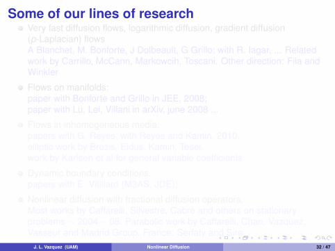
Some of our lines of researchVery fast diffusion flows, logarithmic diffusion, gradient diffusion(p-Laplacian) flowsA Blanchet, M. Bonforte, J Dolbeault, G Grillo; with R. Iagar, ... Relatedwork by Carrillo, McCann, Markowcih, Toscani. Other direction: Fila andWinkler
Flows on manifolds:paper with Bonforte and Grillo in JEE, 2008;paper with Lu, Lei, Villani in arXiv, june 2008 ...
Flows in inhomogeneous media.papers with G. Reyes; with Reyes and Kamin, 2010.elliptic work by Brezis, Eidus, Kamin, Tesei,work by Karlsen et al for general variable coefficients
Dynamic boundary conditions.papers with E. Vitillaro (M3AS, JDE);
Nonlinear diffusion with fractional diffusion operators.Most works by Caffarelli, Silvestre, Cabre and others on stationaryproblems ∼ 2004− 08. Parabolic work by Caffarelli, Chan, Vazquez,Vasseur and Madrid Group. France: Serfaty and Sire.
J. L. Vazquez (UAM) Nonlinear Diffusion 32 / 47

A theorem from 2016This is the main result of a project with Herbert Koch and Clemens Kienzler from Bonn.We solve an open problem posed in 1987, and once the idea was found the projecthas taken a number of years.
Theorem
Let ρ ≥ 0 be a solution of the PME posed for all x ∈ Rn, n ≥ 1, and t > 0, and let theinitial data ρ0 be nonnegative, bounded and compactly supported. Then, there exists atime Tr depending on ρ0 such that for all t > Tr
(i) The free boundary is a C∞ hypersurface close to a ball of radiusR(t) = c1(n,m) M(m−1)λtλ, with λ = 1/(n(m − 1) + 2) (the Barenblatt exponent);(ii) The solution pressure ρm−1(t , x) is a C∞ function inside the support and up to thefree boundary. Moreover, the free boundary function t = h(x) is C∞ in thecomplement of the ball of radius R(Tr ).(iii) Moreover, if the initial mass is M > 0 and the initial function is supported in the ballBR(0), then we can write the upper estimate of the regularization time asTr = T (n,m)Mm−1R2+n(m−1).
The full paper is now in the final touches.We use delicate flatness conditions, scalings, heat semigroups and harmonic analysis.We have eliminated the non-degeneracy condition on the initial data.The estimates are uniform. The result cannot be improved in a number of directions
J. L. Vazquez (UAM) Nonlinear Diffusion 33 / 47
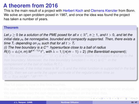

Outline
1 Theories of DiffusionDiffusionHeat equationLinear Parabolic EquationsNonlinear equations
2 Degenerate Diffusion and Free BoundariesIntroductionThe basicsGeneralities
3 Fast Diffusion EquationFast Diffusion Ranges
J. L. Vazquez (UAM) Nonlinear Diffusion 34 / 47
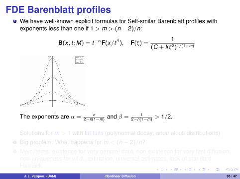
FDE Barenblatt profilesWe have well-known explicit formulas for Self-smilar Barenblatt profiles withexponents less than one if 1 > m > (n − 2)/n:
B(x , t ; M) = t−αF(x/tβ), F(ξ) =1
(C + kξ2)1/(1−m)
The exponents are α = n2−n(1−m)
and β = 12−n(1−m)
> 1/2.
Solutions for m > 1 with fat tails (polynomial decay; anomalous distributions)
Big problem: What happens for m < (n − 2)/n?
Main items: existence for very general data, non-existence for very fast diffusion,non-uniqueness for v.f.d., extinction, universal estimates, lack of standardHarnack.
J. L. Vazquez (UAM) Nonlinear Diffusion 35 / 47

Applied Motivation
J. L. Vazquez (UAM) Nonlinear Diffusion 36 / 47

Carleman model
Simple case of Diffusive limit of kinetic equations. Two types of particles in a onedimensional setting moving with speeds c and −c.Densities are u and v respectively. Dynamics is
(4)
∂tu + c ∂x u = k(u, v)(v − u)
∂tv − c ∂x v = k(u, v)(u − v),
for some interaction kernel k(u, v) ≥ 0. Typical case k = (u + v)αc2.Write now the equations for ρ = u + v and j = c(u − v) and pass to the limitc = 1/ε→∞ and you will obtain to first order in powers or ε = 1/c:
(5)∂ρ
∂t=
12∂
∂x
(1ρα
∂ρ
∂x
),
which is the FDE with m = 1− α, cf. Lions Toscani, 1997. The typical value α = 1gives m = 0, a surprising equation that we will find below! The rigorous investigation ofthe diffusion limit of more complicated particle/kinetic models is an active area ofinvestigation.
J. L. Vazquez (UAM) Nonlinear Diffusion 37 / 47
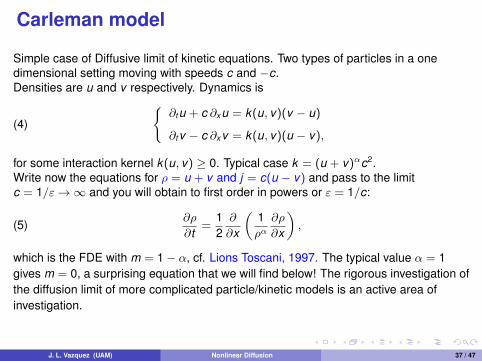

Yamabe problem. EllipticStandard Yamabe problem . We have a Riemannian manifold (M, g0) in spacedimension n ≥ 3, Question: of finding another metric g in the conformal class of g0
having constant scalar curvature.Write the conformal relation as
g = u4/(n−2)g0
locally on M for some positive smooth function u. The conformal factor is u4/(n−2).Denote by R = Rg and R0 the scalar curvatures of the metrics g, g0 resp. Write ∆0 forthe Laplace-Beltrami operator of g0, we have the formula R = −u−NLu on M, withN = (n + 2)/(n − 2) and
Lu := κ∆0u − R0u, κ =4(n − 1)
n − 2.
The Yamabe problem becomes then
(6) ∆0u −(
n − 24(n − 1)
)R0u +
(n − 2
4(n − 1)
)Rgu(n+2)/(n−2) = 0.
The equation should determine u (hence, g) when g0, R0 and Rg are known. In thestandard case we take M = Rn and g0 the standard metric, so that ∆0 is the standardLaplacian, R0 = 0, we take Rg = 1 and then we get the well-known semilinear ellipticequation with critical exponent.
J. L. Vazquez (UAM) Nonlinear Diffusion 38 / 47

Yamabe problem. EvolutionEvolution Yamabe flow is defined as an evolution equation for a family of metrics. Usedas a tool to construct metrics of constant scalar curvature within a given conformalclass. Wwe look for a one-parameter family gt (x) = g(x , t) of metrics solution of theevolution problem
(7) ∂tg = −R g, g(0) = g0 on M.
It is easy to show that this is equivalent to the equation
∂t (uN) = Lu, u(0) = 1 on M.
after rescaling the time variable. Let now (M, g0) be Rn with the standard flat metric, sothat R0 = 0. Put uN = v , m = 1/N = (n − 2)/(n + 2) ∈ (0, 1). Then
(8) ∂tv = Lvm,
which is a fast diffusion equation with exponent my ∈ (0, 1) given by
my =n − 2n + 2
, 1−my =4
n + 2.
If we now try separate variables solutions of the form v(x , t) = (T − t)αf (x), thennecessarily α = 1/(1−my ) = (n + 2)/4, and F = f m satisfies the semilinear ellipticequation with critical exponent that models the stationary version:
(9) ∆F +n + 2
4F
n+2n−2 = 0.
J. L. Vazquez (UAM) Nonlinear Diffusion 39 / 47

Logarithmic Diffusion ISpecial case: the limit case m = 0 of the PME/FDE in two space dimensions
∂tu = div (u−1∇u) = ∆ log(u).
Application to Differential Geometry: it describes the evolution of a conformallyflat metric g given by ds2 = u dr 2 by means of its Ricci curvature:
∂
∂tgij = −2 Ricij = −R gij ,
where Ric is the Ricci tensor and R the scalar curvature.This flow, proposed by R. Hamilton 1 is the equivalent of the Yamabe flow in twodimensions. Remark: what we usually call the mass of the solution (thinking indiffusion terms) becomes here the total area of the surface, A =
∫∫u dx1dx2.
Work on existence, nonuniqueness, extinction, and asymptotics by severalauthors around 1995:Daskalopoulos, Del PinoDi Bendedetto, DillerEsteban, Rodriguez, Vazquez
1RS Hamilton, The Ricci flow on surfaces. Mathematics and general relativity,237–262, Contemp. Math., 71, Amer. Math. Soc., Providence, RI, 1988.
J. L. Vazquez (UAM) Nonlinear Diffusion 40 / 47
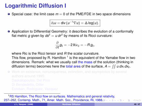

Pictures
About fast diffusion in the limit
Evolution of the ZKB solutions; dimension n = 2.exponent near m = 0
J. L. Vazquez (UAM) Nonlinear Diffusion 41 / 47

Functional Analysis Program
J. L. Vazquez (UAM) Nonlinear Diffusion 42 / 47

Main facts
Existence of an evolution semigroup.
u0 7→ St (u0) = u(t)
A key issue is the choice of functional space.X = L1(Rn) (Brezis, Benilan, Crandall, 1971)Y = L1
loc(Rn) (Herrero, Pierre 1985)M = Locally bounded measures (Pierre, 1987; Dalhberg - Kenig 1988)B = (possibly locally unbounded) Borel mesaures (Chasseigne-Vazquez ARMA2002)
Positivity. Nonnegative data produce positive solutions.
”Smoothing effect”: In many cases Lp → Lq with q > p. Then solutions are C∞
smooth. In other cases, things go wrong (things=Functional Analysis)
Theory for two signs is still poorly understood.Cf. Stefan Problem (Athanasopoulos, Caffarelli, Salsa)
J. L. Vazquez (UAM) Nonlinear Diffusion 43 / 47
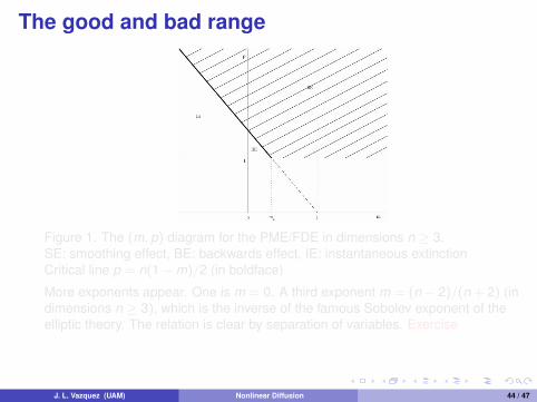
The good and bad range
Figure 1. The (m, p) diagram for the PME/FDE in dimensions n ≥ 3.SE: smoothing effect, BE: backwards effect, IE: instantaneous extinctionCritical line p = n(1−m)/2 (in boldface)
More exponents appear. One is m = 0. A third exponent m = (n − 2)/(n + 2) (indimensions n ≥ 3), which is the inverse of the famous Sobolev exponent of theelliptic theory. The relation is clear by separation of variables. Exercise
J. L. Vazquez (UAM) Nonlinear Diffusion 44 / 47
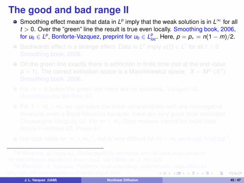
The good and bad range IISmoothing effect means that data in Lp imply that the weak solution is in L∞ for allt > 0. Over the ”green” line the result is true even locally. Smoothing book, 2006,for u0 ∈ Lp, Bonforte-Vazquez, preprint for u0 ∈ Lp
loc . Here, p = p∗ = n(1−m)/2.
Backwards effect is a strange effect. Data in Lp imply u(t) ∈ L1 for all t > 0Smoothing book, 2006.
On the green line exactly there is extinction in finite time (not at the end valuep = 1). The correct extinction space is a Marcinkiewicz space: X = Mp∗(Rn)Smoothing book, 2006.
For m < 0 below the green line there are no solutions. Vazquez 92,Daskalopoulos del Pino 97.
For 1 > m > mc we can solve the initial value problem with any nonnegativemeasure, even a Borel Measure because there are very good local estimatesChasseigne-Vazquez 03. For m < mc Dirac masses cannot be initial dataBrezis-Friedman 83, Pierre 87.
Harnack holds for m > mc2, but is very difficult for m < mc work just finished 3.
2M Bonforte- JL Vazquez, Global positivity estimates and Harnack inequalities forthe fast diffusion equation.J. Funct. Anal. 240 (2006), no. 2, 399–428
3M Bonforte- JL Vazquez, Positivity, local smoothing, and Harnack inequalities forvery fast diffusion equations, Preprint March 2008
J. L. Vazquez (UAM) Nonlinear Diffusion 45 / 47
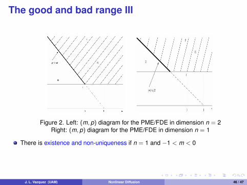
The good and bad range III
Figure 2. Left: (m, p) diagram for the PME/FDE in dimension n = 2Right: (m, p) diagram for the PME/FDE in dimension n = 1
There is existence and non-uniqueness if n = 1 and −1 < m < 0
J. L. Vazquez (UAM) Nonlinear Diffusion 46 / 47

The Fast Diffusion Equation is a long story.
Let us put the End here
Thank you
♠ ♠ ♠
Gracias, Grazie
J. L. Vazquez (UAM) Nonlinear Diffusion 47 / 47

The Fast Diffusion Equation is a long story.
Let us put the End here
Thank you
♠ ♠ ♠
Gracias, Grazie
J. L. Vazquez (UAM) Nonlinear Diffusion 47 / 47
The Fast Diffusion Equation is a long story.
Let us put the End here
Thank you
♠ ♠ ♠
Gracias, Grazie
J. L. Vazquez (UAM) Nonlinear Diffusion 47 / 47

The Fast Diffusion Equation is a long story.
Let us put the End here
Thank you
♠ ♠ ♠
Gracias, Grazie
J. L. Vazquez (UAM) Nonlinear Diffusion 47 / 47
The Fast Diffusion Equation is a long story.
Let us put the End here
Thank you
♠ ♠ ♠
Gracias, Grazie
J. L. Vazquez (UAM) Nonlinear Diffusion 47 / 47

1
The theory of nonlinear diffusionwith fractional operators
JUAN LUIS VAZQUEZ
Departamento de MatematicasUniversidad Autonoma de Madridand Royal Academy of Sciences
CIME Summer Course“Nonlocal and Nonlinear Diffusions and
Interactions: New Methods and Directions”
Cetraro, Italia July 4, 2016

2
Outline
1 Linear and Nonlinear DiffusionNonlinear equations
2 Fractional diffusion
3 Nonlinear Fractional diffusion modelsModel I. A potential Fractional diffusionMain estimates for this model

3
Outline
1 Linear and Nonlinear DiffusionNonlinear equations
2 Fractional diffusion
3 Nonlinear Fractional diffusion modelsModel I. A potential Fractional diffusionMain estimates for this model

Outline
1 Linear and Nonlinear DiffusionNonlinear equations
2 Fractional diffusion
3 Nonlinear Fractional diffusion modelsModel I. A potential Fractional diffusionMain estimates for this model

5
Diffusion equations describe how a continuous medium(say, a population) spreads to occupy the available space.Models come from all kinds of applications: fluids,chemicals, bacteria, animal populations, the stock market,...These equations have occupied a large part of my research since 1980.
The mathematical study of diffusion starts with the HeatEquation,
ut = ∆ua linear example of immense influence in Science.The Heat Equation has produced a huge number of concepts,techniques and connections for pure and applied science, for analysts,probabilists, computational people and geometers, for physicists andengineers, and lately in finance and the social sciences.Today educated people talk about the Gaussian function, separation ofvariables, Fourier analysis, spectral decomposition, Dirichlet forms,Maximum Principles, Brownian motion, generation of semigroups,positive operators in Banach spaces, entropy dissipation, ...
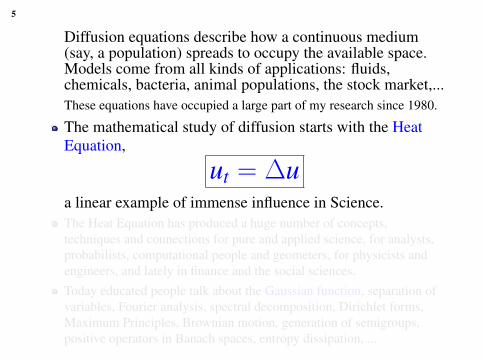

6
Nonlinear equations
The heat example is generalized into the theory of linear parabolicequations, which is nowadays a basic topic in any advanced study ofPDEs.However, the heat example and the linear models are not representativeenough, since many models of science are nonlinear in a form that isvery not-linear. A general model of nonlinear diffusion takes thedivergence form
∂tH(u) = ∇ · ~A(x, u,Du) + B(x, t, u,Du)
with monotonicity conditions on H and ∇p ~A(x, t, u, p) and structuralconditions on ~A and B. Posed in the 1960s (Serrin et al.)In this generality the mathematical theory is too rich to admit a simpledescription. This includes the big areas of Nonlinear Diffusion andReaction Diffusion, where I have been working.Reference works. Books by Ladyzhenskaya-Solonnikov-Uraltseva,Friedman, Smoller,... But they are only basic reference.
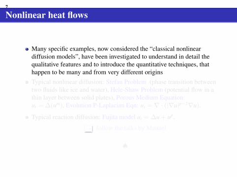
7
Nonlinear heat flows
Many specific examples, now considered the “classical nonlineardiffusion models”, have been investigated to understand in detail thequalitative features and to introduce the quantitative techniques, thathappen to be many and from very different originsTypical nonlinear diffusion: Stefan Problem (phase transition betweentwo fluids like ice and water), Hele-Shaw Problem (potential flow in athin layer between solid plates), Porous Medium Equation:ut = ∆(um), Evolution P-Laplacian Eqn: ut = ∇ · (|∇u|p−2∇u).
Typical reaction diffusion: Fujita model ut = ∆u + up.
→ follow the talks by Manuel
♠

8
Outline
1 Linear and Nonlinear DiffusionNonlinear equations
2 Fractional diffusion
3 Nonlinear Fractional diffusion modelsModel I. A potential Fractional diffusionMain estimates for this model

9
Recent Direction. Fractional diffusion
Replacing Laplacians by fractional Laplacians is motivated by the need torepresent anomalous diffusion. In probabilistic terms, it replacesnext-neighbour interaction of Random Walks and their limit, the Brownianmotion, by long-distance interaction. The main mathematical models are theFractional Laplacians that have special symmetry and invariance properties.
The Basic evolution equation
ut + (−∆)su = 0
Intense work in Stochastic Processes for some decades, but not in Analysis ofPDEs until 10 years ago, initiated around Prof. Caffarelli in Texas.
A basic theory and survey for PDE people: M. Bonforte, Y. Sire, J. L. Vazquez.“Optimal Existence and Uniqueness Theory for the Fractional Heat Equation”,Arxiv:1606.00873v1 [math.AP], to appear.
Precedent : B. Barrios, I. Peral, F. Soria, E. Valdinoci. “A Widder’s typetheorem for the heat equation with nonlocal diffusion” Arch. Ration. Mech.Anal. 213 (2014), no. 2, 629–650.
10
The fractional Laplacian operator
Different formulas for fractional Laplacian operator.We assume that the space variable x ∈ Rn, and the fractional exponentis 0 < s < 1. First, pseudo differential operator given by the Fourier transform:
(−∆)su(ξ) = |ξ|2su(ξ)
Singular integral operator:
(−∆)su(x) = Cn,s
∫Rn
u(x)− u(y)
|x− y|n+2s dy
With this definition, it is the inverse of the Riesz integral operator (−∆)−su.This one has kernel C1|x− y|n−2s, which is not integrable.Take the random walk for Levy processes:
un+1j =
∑k
Pjkunk
where Pik denotes the transition function which has a . tail (i.e, power decaywith the distance |i− k|). In the limit you get an operator A as the infinitesimalgenerator of a Levy process: if Xt is the isotropic α-stable Levy process we have
Au(x) = limh→0
E(u(x)− u(x + Xh))

11
The fractional Laplacian operator II
The α-harmonic extension: Find first the solution of the (n + 1) problem
∇ · (y1−α∇v) = 0 (x, y) ∈ Rn × R+; v(x, 0) = u(x), x ∈ Rn.
Then, putting α = 2s we have
(−∆)su(x) = −Cα limy→0
y1−α ∂v∂y
When s = 1/2 i.e. α = 1, the extended function v is harmonic (in n + 1variables) and the operator is the Dirichlet-to-Neumann map on the base spacex ∈ Rn. It was proposed in PDEs by Caffarelli and Silvestre.
Remark. In Rn all these versions are equivalent. In a bounded domain we haveto re-examine all of them. Three main alternatives are studied in probability andPDEs, corresponding to different options about what happens to particles at theboundary or what is the domain of the functionals.
References. Books by Landkof (1966-72), Stein (1970), Davies (1996).
12
Outline
1 Linear and Nonlinear DiffusionNonlinear equations
2 Fractional diffusion
3 Nonlinear Fractional diffusion modelsModel I. A potential Fractional diffusionMain estimates for this model

13
Nonlocal nonlinear diffusion model I
The model arises from the consideration of a continuum, say, a fluid,represented by a density distribution u(x, t) ≥ 0 that evolves with timefollowing a velocity field v(x, t), according to the continuity equation
ut +∇ · (u v) = 0.
We assume next that v derives from a potential, v = −∇p, as happens in fluidsin porous media according to Darcy’s law, an in that case p is the pressure. Butpotential velocity fields are found in many other instances, like Hele-Shawcells, and other recent examples.
We still need a closure relation to relate u and p. In the case of gases in porousmedia, as modeled by Leibenzon and Muskat, the closure relation takes theform of a state law p = f (u), where f is a nondecreasing scalar function, whichis linear when the flow is isothermal, and a power of u if it is adiabatic.The linear relationship happens also in the simplified description of waterinfiltration in an almost horizontal soil layer according to Boussinesq. In bothcases we get the standard porous medium equation, ut = c∆(u2).See PME Book for these and other applications (around 20!).
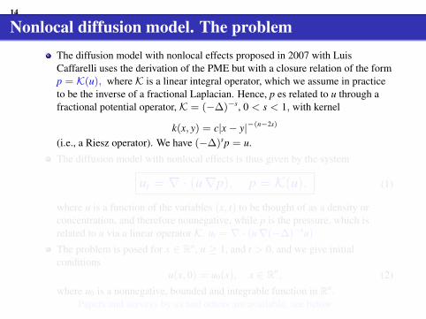
14
Nonlocal diffusion model. The problemThe diffusion model with nonlocal effects proposed in 2007 with LuisCaffarelli uses the derivation of the PME but with a closure relation of the formp = K(u), where K is a linear integral operator, which we assume in practiceto be the inverse of a fractional Laplacian. Hence, p es related to u through afractional potential operator, K = (−∆)−s, 0 < s < 1, with kernel
k(x, y) = c|x− y|−(n−2s)
(i.e., a Riesz operator). We have (−∆)sp = u.
The diffusion model with nonlocal effects is thus given by the system
ut = ∇ · (u∇p), p = K(u). (1)
where u is a function of the variables (x, t) to be thought of as a density orconcentration, and therefore nonnegative, while p is the pressure, which isrelated to u via a linear operator K. ut = ∇ · (u∇(−∆)−su)
The problem is posed for x ∈ Rn, n ≥ 1, and t > 0, and we give initialconditions
u(x, 0) = u0(x), x ∈ Rn, (2)
where u0 is a nonnegative, bounded and integrable function in Rn.Papers and surveys by us and others are available, see below
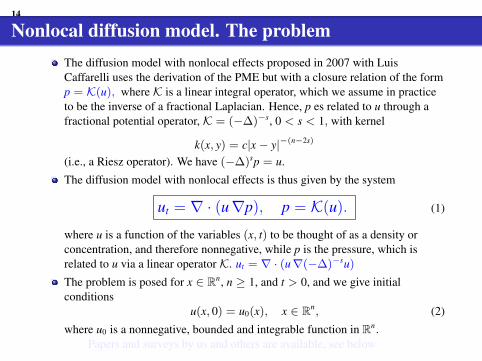

15
Nonlocal diffusion model
The interest in using fractional Laplacians in modeling diffusive processes has awide literature, especially when one wants to model long-range diffusiveinteraction, and this interest has been activated by the recent progress in themathematical theory as a large number works on elliptic equations, mainly ofthe linear or semilinear type (Caffarelli school; Bass, Kassmann, and others)
There are many works on the subject. Here is a good reference to fractionalelliptic work by a young Spanish authorXavier Ros-Oton. Nonlocal elliptic equations in bounded domains: a survey,Preprint in arXiv:1504.04099 [math.AP].

16
Nonlocal diffusion Model I. ApplicationsModeling dislocation dynamics as a continuum. This has been studied by P.Biler, G. Karch, and R. Monneau (2008), and then other collaborators,following old modeling by A. K. Head on Dislocation group dynamics II.Similarity solutions of the continuum approximation. (1972).This is a one-dimensional model. By integration in x they introduce viscositysolutions a la Crandall-Evans-Lions. Uniqueness holds.Equations of the more general form ut = ∇ · (σ(u)∇Lu) have appearedrecently in a number of applications in particle physics. Thus, Giacomin andLebowitz (J. Stat. Phys. (1997)) consider a lattice gas with general short-rangeinteractions and a Kac potential, and passing to the limit, the macroscopicdensity profile ρ(r, t) satisfies the equation
∂ρ
∂t= ∇ ·
[σs(ρ)∇δF(ρ)
δρ
]See also (GL2) and the review paper (GLP). The model is used to study phasesegregation in (GLM, 2000).More generally, it could be assumed that K is an operator of integral typedefined by convolution on all of Rn, with the assumptions that is positive andsymmetric. The fact the K is a homogeneous operator of degree 2s, 0 < s < 1,will be important in the proofs. An interesting variant would be the Besselkernel K = (−∆ + cI)−s. We are not exploring such extensions.

17
Extreme cases
If we take s = 0, K = the identity operator, we get the standard porous mediumequation, whose behaviour is well-known, see references later.
In the other end of the s interval, when s = 1 and we take K = −∆ we get
ut = ∇u · ∇p− u2, −∆p = u. (3)
In one dimension this leads to ut = uxpx − u2, pxx = −u. In terms ofv = −px =
∫u dx we have
vt = upx + c(t) = −vxv + c(t),
For c = 0 this is the Burgers equation vt + vvx = 0 which generates shocks infinite time but only if we allow for u to have two signs.
HYDRODYNAMIC LIMIT. The case s = 1 in several dimensions is moreinteresting because it does not reduce to a simple Burgers equation.
ut = ∇ · (u∇p) = ∇u · ∇p− u2; , p = (−∆)−1u ,
Applications in superconductivity and superfluidity, see paper with Serfaty andbelow.

18
Our first project. Results
Existence of weak energy solutions and property of finite propagationL. Caffarelli and J. L. Vazquez, Nonlinear porous medium flow withfractional potential pressure, Arch. Rational Mech. Anal. 2011; arXiv2010.
Existence of self-similar profiles, renormalized Fokker-Planck equationand entropy-based proof of stabilizationL. Caffarelli and J. L. Vazquez, Asymptotic behaviour of a porousmedium equation with fractional diffusion, appeared in Discrete Cont.Dynam. Systems, 2011; arXiv 2010.
Regularity in three levels: L1 → L2, L2 → L∞, and bounded implies Cα
L. Caffarelli, F. Soria, and J. L. Vazquez, Regularity of porous mediumequation with fractional diffusion, J. Eur. Math. Soc. (JEMS) 15 5(2013), 1701–1746. The very subtle case s = 1/2 is solved in a newpaper L. Caffarelli, and J. L. Vazquez, appeared in ArXiv and asNewton Institute Preprint, 2014
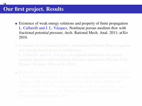
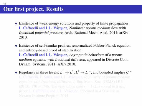
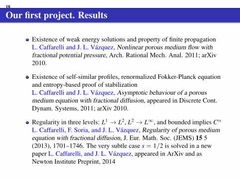
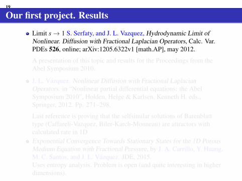
19
Our first project. Results
Limit s→ 1 S. Serfaty, and J. L. Vazquez, Hydrodynamic Limit ofNonlinear. Diffusion with Fractional Laplacian Operators, Calc. Var.PDEs 526, online; arXiv:1205.6322v1 [math.AP], may 2012.
A presentation of this topic and results for the Proceedings from theAbel Symposium 2010.
J. L. Vazquez. Nonlinear Diffusion with Fractional LaplacianOperators. in “Nonlinear partial differential equations: the AbelSymposium 2010”, Holden, Helge & Karlsen, Kenneth H. eds.,Springer, 2012. Pp. 271–298.
Last reference is proving that the selfsimilar solutions of Barenblatttype (Caffareli-Vazquez, Biler-Karch-Monneau) are attractors withcalculated rate in 1DExponential Convergence Towards Stationary States for the 1D PorousMedium Equation with Fractional Pressure, by J. A. Carrillo, Y. Huang,M. C. Santos, and J. L. Vazquez. JDE, 2015.Uses entropy analysis. Problem is open (and quite interesting in higherdimensions).
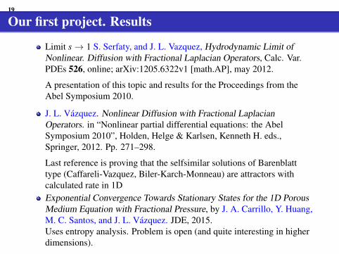

20
Main estimates for this model
We recall that the equation of M1 is ∂tu = ∇ · (u∇K(u)), posed in the wholespace Rn.We consider K = (−∆)−s for some 0 < s < 1 acting on Schwartz classfunctions defined in the whole space. It is a positive essentially self-adjointoperator. We let H = K1/2 = (−∆)−s/2.We do next formal calculations, assuming that u ≥ 0 satisfies the requiredsmoothness and integrability assumptions. This is to be justified later byapproximation.
Conservation of massddt
∫u(x, t) dx = 0. (4)
First energy estimate:
ddt
∫u(x, t) log u(x, t) dx = −
∫|∇Hu|2 dx. (5)
Second energy estimate
ddt
∫|Hu(x, t)|2 dx = −2
∫u|∇Ku|2 dx. (6)
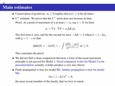
21
Main estimatesConservation of positivity: u0 ≥ 0 implies that u(t) ≥ 0 for all times.
L∞ estimate. We prove that the L∞ norm does not increase in time.Proof. At a point of maximum of u at time t = t0, say x = 0, we have
ut = ∇u · ∇P + u ∆K(u).
The first term is zero, and for the second we have −∆K = L where L = (−∆)q
with q = 1− s so that
∆Ku(0) = −Lu(0) = −∫
u(0)− u(y)
|y|n+2(1−s) dy ≤ 0.
This concludes the proof.
We did not find a clean comparison theorem, a form of the usual maximumprinciple is not proved for Model 1. Good comparion works for Model 2 to bepresented below, actually, it helps produce a very nice theory.
Finite propagation is true for model M1. Infinite propagation is true for modelM2.
∂tu + (−∆)sum = 0,
the most recent member of the family, that we love so much.

22
Boundedness
Solutions are bounded in terms of data in Lp, 1 ≤ p ≤ ∞.For Model 1 Use (the de Giorgi or the Moser) iteration technique on theCaffarelli-Silvestre extension as in Caffarelli-Vasseur.Or use energy estimates based on the properties of the quadratic andbilinear forms associated to the fractional operator, and then theiteration technique
Theorem (for M1) Let u be a weak solution the IVP for the FPMEwith data u0 ∈ L1(Rn) ∩ L∞(Rn), as constructed before. Then, thereexists a positive constant C such that for every t > 0
supx∈Rn|u(x, t)| ≤ C t−α‖u0‖γL1(Rn)
(7)
with α = n/(n + 2− 2s), γ = (2− 2s)/((n + 2− 2s). The constant Cdepends only on n and s.This theorem allows to extend the theory to data u0 ∈ L1(Rn), u0 ≥ 0,with global existence of bounded weak solutions.
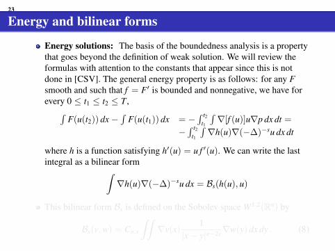
23
Energy and bilinear forms
Energy solutions: The basis of the boundedness analysis is a propertythat goes beyond the definition of weak solution. We will review theformulas with attention to the constants that appear since this is notdone in [CSV]. The general energy property is as follows: for any Fsmooth and such that f = F′ is bounded and nonnegative, we have forevery 0 ≤ t1 ≤ t2 ≤ T ,∫
F(u(t2)) dx−∫
F(u(t1)) dx = −∫ t2
t1
∫∇[f (u)]u∇p dx dt =
−∫ t2
t1
∫∇h(u)∇(−∆)−su dx dt
where h is a function satisfying h′(u) = u f ′(u). We can write the lastintegral as a bilinear form∫
∇h(u)∇(−∆)−su dx = Bs(h(u), u)
This bilinear form Bs is defined on the Sobolev space W1,2(Rn) by
Bs(v,w) = Cn,s
∫∫∇v(x)
1|x− y|n−2s∇w(y) dx dy . (8)
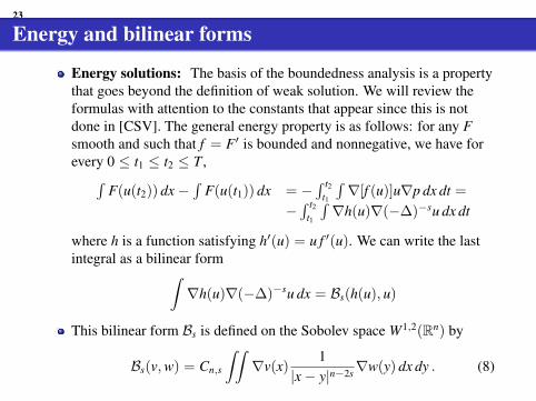

24
Energy and bilinear forms II
This bilinear form Bs is defined on the Sobolev space W1,2(Rn) by
Bs(v,w) = Cn,s∫∫∇v(x) 1
|x−y|n−2s∇w(y) dx dy =∫∫N−s(x, y)∇v(x)∇w(y) dx dy
where N−s(x, y) = Cn,s|x− y|−(n−2s) is the kernel of operator (−∆)−s.After some integrations by parts we also have
Bs(v,w) = Cn,1−s
∫∫(v(x)− v(y))
1|x− y|n+2(1−s) (w(x)− w(y)) dx dy
(9)since −∆N−s = N1−s.It is known (Stein) that Bs(u, u) is an equivalent norm for the fractionalSobolev space W1−s,2(Rn).We will need in the proofs that Cn,1−s ∼ Kn(1− s) as s→ 1, for someconstant Kn depending only on n.

25
Additional and Recent work, open problems
The asymptotic behaviour as t→∞ is a very interesting topicdeveloped in a paper with Luis Caffarelli. Rates of convergence arefound for in dimension n = 1 but they are not available for n > 1, theyare tied to some functional inequalities that are not known.The study of the free boundary is in progress, but it is still open forsmall s > 0.The equation is generalized into ut = ∇ · (um−1∇(−∆)−su) withm > 1. Recent work with D. Stan and F. del Teso shows that finitepropagation is true for m ≥ 2 and propagation is infinite is m < 2. Thisis quite different from the standard porous medium case s = 0, wherem = 1 is the dividing value.Gradient flow in Wasserstein metrics is work by S. Lisini, E. Maininiand A. Segatti, just appeared in arXiv, A gradient flow approach to theporous medium equation with fractional pressure. Thanks to the Paviapeople!Previous work by J. A. Carrillo et al. in n = 1.
26
The questions of uniqueness and comparison are solved in dimensionn = 1 thanks to the trick of integration in space used by Biler, Karch,and Monneau. New tools are needed to make progress in severaldimensions.Recent uniqueness results. Paper by X H Zhou, W L Xiao, J C Chen,Fractional porous medium and mean field equations in Besov spaces,EJDE 2014. They obtain local in time strong solutions in Besov spaces.Thus, for initial data in Bα1,∞ if 1/2 ≤ s < 1 and α > n + 1 and n ≥ 2.The problem in a bounded domain with Dirichlet or Neumann data hasnot been studied.Good numerical studies are needed.
27
Most of the recent effort by me and collaborators has been devoted tothe parallel model
ut + (−∆)sum = 0
which does not have an entropy theory. However, it generates asemigroup of contractions in L1(Rn). This needs a whole new lecture
The theory in bounded domains is being developed just now, I mentionmy collaborators M. Bonforte and Y. Sire, and among other groups, E.Valdinoci and coauthors (mostly elliptic).
(Go to arXiv, the consolation of the learning masses)

28
The End
Thank you, Gracias, Grazie

28
The End
Thank you, Gracias, Grazie

28
The End
Thank you, Gracias, Grazie

Entropies for Nonlinear diffusionequations
JUAN LUIS VAZQUEZ
Departamento de MatematicasUniversidad Autonoma de Madridand Royal Academy of Sciences
CIME Summer Course“Nonlocal and Nonlinear Diffusions and
Interactions: New Methods and Directions”Cetraro, Italia July 4, 2016
J. L. Vazquez (UAM) Nonlinear Diffusion 1 / 31

Outline
1 Estimates for the Heat EquationsHeat Equation Methods
2 Traditional porous mediumAsymptotic behaviourThe Fast Diffusion Problem in RN
3 Nonlinear Fractional diffusionIntroduction to Fractional diffusionAsymptotic behavior for the nonlocal HE / PMERenormalized estimates
J. L. Vazquez (UAM) Nonlinear Diffusion 2 / 31

Energy estimates
We are going to use energy functions of different types to study the evolution ofdissipation equations.
The basic equation is the classical heat equation, but the scope is quite general.Our aim is not to establish the convergence of general solutions to thefundamental solution (which is well done by other methods), but a bit more: tofind the speed of convergence. After change of variables (renormalization) thisreads as rate of convergence to equilibrium and relies on important functionalinequalities.
The methods will apply to more general linear parabolic equations that generatesemigroups. The method works for equations evolving on manifolds as a basespace.
Since 2000 we have been studying nonlinear diffusion equations.
Nonlinear models: porous medium equation, fast diffusion equation,p-Laplacian evolution equation, chemotaxis system, thin films, ...
plusfractional heat equation and fractional porous medium equations (since 2007), ...
J. L. Vazquez (UAM) Nonlinear Diffusion 3 / 31

Energy estimates for the Heat EquationTake the classical Heat Equation posed in the whole space RN for τ > 0:
uτ =12
∆y u
with notation u = u(y , τ) that is useful as we will see. We know the (self-similar)fundamental solution, that is an attractor of its basin
U(y , τ) = C τ−N/2e−y2/2τ .
First step: the logarithmic time-space rescaling
u(y , τ) = v(x , t) (1 + τ)−N/2, y = x(1 + τ)1/2, t = log(1 + τ),
that leads to the well-known Fokker-Plank equation for v(x , t):
vt =12
∆x v +12∇ · (x v)
If we now pass to the quotient w = v/G, where G = c e−x2/2 is the stationarystate (Gaussiann kernel), to get the Ornstein-Uhlenbeck version
wt =12
G−1∇ ·(
G∇w),
a symmetrically weighted heat equation. The equivalence of these threeequations is a main tool in Linear Diffusion and Semigroup Theory.
J. L. Vazquez (UAM) Nonlinear Diffusion 4 / 31
Energy estimates for the Heat Equation IIWe may assume without lack of generality that
∫w dµ =
∫v dx =
∫u dy = 1.
We now make a crucial estimate on the time decay of the energy for the OUE:
F(w(t)) =
∫RN|w − 1|2 G dx ,
dF(w(t))
dt= −
∫RN|∇w |2 G dx = −D(w(t)).
We can now use a result from abstract functional analysis: the Gaussian Poincareinequality with measure dµ = G(x) dx :∫
RNw2dµ−
(∫RN
w dµ)2)≤∫RN|∇w |2 dµ
Then, the Left Hand Side is just F and the inequality implies after integration that:∫RN|w − 1|2 dµ ≤ e−t
∫Rd|w0 − 1|2 dµ ∀ t ≥ 0
Then by regularity theory, we get ‖w − 1‖∞ ≤ Ke−t , that means, once we goback to the original variables that:
(1− Ce−t )G(x , t) ≤ v(x , t) ≤ (1 + Ce−t ) G(x) (e−t =1
1 + τ).
These are the well known Heat Kernel Estimates of solutions to the HE.
J. L. Vazquez (UAM) Nonlinear Diffusion 5 / 31
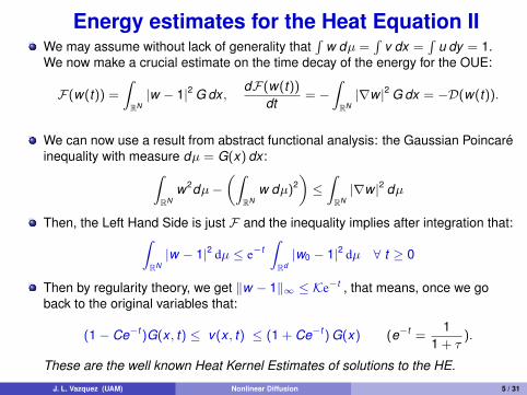

Entropy estimates for the Heat Equation IIIThere is another approach that starts the analysis from Boltzmann’s ideas onentropy dissipation. We start from the Fokker-Planck equation vt = ∆v +∇ · (xv)and consider the functional called entropy
E(v) =
∫RN
v log(v/G) dx =
∫RN
v log(v)dx +12
∫RN
x2v dx + C .
Differentiating along the flow (i.e., for a solution) leads to
dE(v)
dt= −I(v), I(u) =
∫RN
v |∇vv
+ x |2 dx =
∫RN
v |∇ log(v/G)|2 dx .
Put now v = Gf 2 to find that
E(v) = 2∫RN
f 2 log(f ) dx , I(v) = 4∫RN|∇f |2 dx
The famous logarithmic Sobolev inequality [Gross 75] says than that (for allfunctions, not only solutions)
E ≤ 12I
and we obtain the decay E(t) ≤ E(0) e−2t . Translate that into a good norm.
J. L. Vazquez (UAM) Nonlinear Diffusion 6 / 31

About entropy in physics
Entropy has been introduced as a state function in thermodynamics by R.Clausius in 1865, in the framework of the second law of thermodynamics, in orderto interpret the results of S. Carnot.
A statistical physics approach: Boltzmann’s formula (1877) defines the entropy ofa system in terms of a counting of the micro-states of a physical system.Boltzmann’s equation: ∂t f + v · ∇x f = Q(f , f ). It describes the evolution of a gasof particles having binary collisions at the kinetic level; f (t , x , v) is a timedependent distribution function (probability density) defined on the phase spaceRN × RN .
The Boltzmann entropy: H[f ] :=∫∫
f log(f )dxdv measures irreversibility:The famous H-Theorem (1872) says that
ddt
H[f ] =
∫∫Q(f , f )log(f )dxdv ≤ 0 .
Other notions of entropy: The Shannon entropy in information theory, entropy inprobability theory (with reference to an arbitrary measure).Other approaches: Caratheodory (1908), Lieb-Yngvason (1997).
J. L. Vazquez (UAM) Nonlinear Diffusion 7 / 31

Porous Medium / Fast Diffusion Equations
The simplest model of nonlinear diffusion equation is maybe
ut = ∆um = ∇ · (c(u)∇u)
c(u) indicates density-dependent diffusivity
c(u) = mum−1[= m|u|m−1]
If m > 1 it degenerates at u = 0 , =⇒ slow diffusion
For m = 1 we get the classical Heat Equation.
On the contrary, if m < 1 it is singular at u = 0 =⇒ Fast Diffusion.
A more general model of nonlinear diffusion takes the divergence form
∂tH(u) = ∇ · ~A(x , u,Du) + B(x , t , u,Du)
with monotonicity conditions on H and ∇p ~A(x , t , u, p) and structural conditions on~A and B. This generality includes Stefan Problems, p-Laplacian flows (includingp =∞ and total variation flow p = 1) and many others.
J. L. Vazquez (UAM) Nonlinear Diffusion 8 / 31

Barenblatt profiles and Asymptotics
These profiles are the alternative to the Gaussian profiles that have star role forthe HE.
They are source solutions. Source means that u(x , t)→ M δ(x) as t → 0. usExplicit formulas (1950, 52) are self-similar:
B(x , t ;M) = t−αF(x/tβ), F(ξ) =(
C − kξ2)1/(m−1)
+
α = n2+n(m−1)
β = 12+n(m−1) < 1/2
Height u = Ct−α
Free boundary at distance |x | = ctβ
Scaling law; anomalous diffusion versus Brownian motion.
J. L. Vazquez (UAM) Nonlinear Diffusion 9 / 31
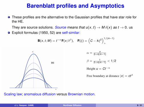
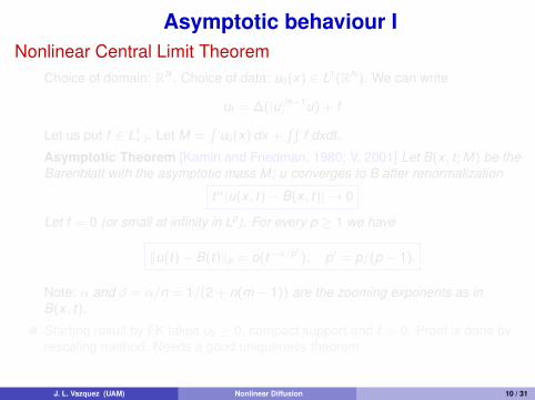
Asymptotic behaviour INonlinear Central Limit Theorem
Choice of domain: RN . Choice of data: u0(x) ∈ L1(RN). We can write
ut = ∆(|u|m−1u) + f
Let us put f ∈ L1x,t . Let M =
∫u0(x) dx +
∫∫f dxdt .
Asymptotic Theorem [Kamin and Friedman, 1980; V. 2001] Let B(x , t ; M) be theBarenblatt with the asymptotic mass M; u converges to B after renormalization
tα|u(x , t)− B(x , t)| → 0
Let f = 0 (or small at infinity in Lp). For every p ≥ 1 we have
‖u(t)− B(t)‖p = o(t−α/p′), p′ = p/(p − 1).
Note: α and β = α/n = 1/(2 + n(m − 1)) are the zooming exponents as inB(x , t).
Starting result by FK takes u0 ≥ 0, compact support and f = 0. Proof is done byrescaling method. Needs a good uniqueness theorem.
J. L. Vazquez (UAM) Nonlinear Diffusion 10 / 31
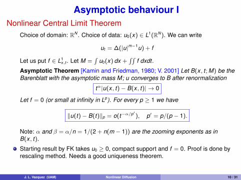

Calculations of the entropy ratesThis is next step of information after plain convergence.We rescale the function as u(x , t) = r(t)n ρ(y r(t), s)
where r(t) is the Barenblatt radius at t + 1, and “new time” is s = log(1 + t).Equation becomes
ρs = div (ρ(∇ρm−1 +c2∇y2)).
Then define a new entropy (not Boltzmann entropy, but a new type called Renyientropy)
E(u)(t) =
∫(
1mρm +
c2ρy2) dy
The minimum of entropy is identified as the Barenblatt profile.Calculate
dEds
= −∫ρ|∇ρm−1 + cy |2 dy = −D
Moreover, a calculation known as Bakry-Emery gives
dDds
= −R, R ∼ λD.
We conclude exponential decay of D in new time s, i.e., a power rate in real timet. It follows that E decays to a minimum E∞ > 0 and we then prove that this is thelevel of the Barenblatt solution, which attains the functional minimum.
J. L. Vazquez (UAM) Nonlinear Diffusion 11 / 31
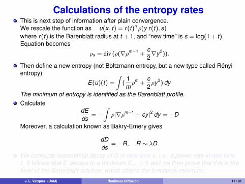

Cauchy Problem for the Fast Diffusion Equation
We consider the model problem in RN
∂τu = ∆
(um
m
)= ∇ ·
(um−1∇u
), (τ, y) ∈ (0,T )× RN
u(0, ·) = u0 , u0 ∈ L1loc
(RN)
for any m < 1 ( i.e. Fast Diffusion, FDE )
We consider non-negative initial data and solutions.
Note that m ≤ 0 is included and m = 0 corresponds to logarithmic diffusion.
Existence and uniqueness of weak solutions by Herrero and Pierre (1985).
Solutions have different behaviour if mc < m < 1 and if m < mc , where
mc :=N − 2
N, and mc > 0 ⇐⇒ N ≥ 3
J. L. Vazquez (UAM) Nonlinear Diffusion 12 / 31

Rates through entropies for Fast Diffusion
Large effort has been invested in making the entropy machinery work for fast diffusion,−∞ < m < 1.
The nice properties of the entropies from the view of transport theory (cf. Villani’s book)are lost soon, when m = (N − 1)/N.
Finite entropy is lost when the second moment is infinite, i.e. for m = (N − 1)/(N + 1).
Finite-mass, stable states (Barenblatt solutions) are lost for m = (N − 2)/N.
Functional inequalities play a crucial role in the asymptotic analysis, there are so to say“equivalent”.
There is work by many authors: Blanchet, Bonforte, Carrillo, Dolbeault, Del Pino, Den-zler, Grillo, McCann, Markowich, Otto, Slepcev, Vazquez, ...
J. L. Vazquez (UAM) Nonlinear Diffusion 13 / 31
References to our work
Juan Luis Vazquez, “Smoothing and decay estimates for nonlinear diffusionequations. Equations of porous medium type”. Oxford Lecture Series inMathematics and its Applications, 33. Oxford University Press, Oxford, 2006.
M.B., J. L. Vazquez, Global positivity estimates and Harnack inequalities for thefast diffusion equation, J. Funct. Anal., 240 (2006), pp. 399–428.
A. Blanchet, M.B., J. Dolbeault, G. Grillo, J. L. Vazquez, Hardy-Poincare inequalitiesand applications to nonlinear diffusions, C. R. Math. Acad. Sci. Paris, 344 (2007),431–436.
A. Blanchet, M.B., J. Dolbeault, G. Grillo, J. L. Vazquez, Asymptotics of the fastdiffusion equation via entropy estimates, Arch. Rat. Mech. Anal. 191 (2009),347–385.
M.B., J. Dolbeault, G. Grillo, J. L. Vazquez, Sharp rates of decay of solutions to thenonlinear fast diffusion equation via functional inequalities, PNAS (Proc. Nat. Acad.Sci.), 107 n. 38, (2010) 16459–16464.
M.B., G. Grillo, J. L. Vazquez, Special fast diffusion with slow asymptotics. Entropymethod and flow on a Riemannian manifold, Arch. Rat. Mech. Anal. 196, (2010),631–680
J. L. Vazquez (UAM) Nonlinear Diffusion 14 / 31

Nonlocal diffusion
Fractional diffusion
Nonlinear Models and Entropies
J. L. Vazquez (UAM) Nonlinear Diffusion 15 / 31

Fractional diffusion
Replacing Laplacians by fractional Laplacians is motivated by the need torepresent anomalous diffusion. In probabilistic terms it replaces next-neighbourinteraction and Brownian motion by long-distance interaction. The mainmathematical models are the Fractional Laplacians that have special symmetryand invariance properties.
Basic evolution equation
∂tu + (−∆)su = 0
Intense work in Stochastic Processes for some decades, but not in Analysis ofPDEs until 10 years ago, initiated around Prof. Caffarelli in Texas.
A basic theory and survey for PDE people: M. Bonforte, Y. Sire, J. L. Vazquez.“Optimal Existence and Uniqueness Theory for the Fractional Heat Equation”,Arxiv:1606.00873v1 [math.AP], to appear.
J. L. Vazquez (UAM) Nonlinear Diffusion 16 / 31
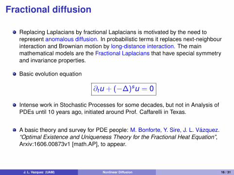
Asymptotic behavior
for the nonlocal PME 1
1Asymptotic behavior of a porous medium equation with fractional diffusion,Luis Caffarelli, Juan Luis Vazquez, Discrete Cont. Dynam. Systems, special issue 2011.
J. L. Vazquez (UAM) Nonlinear Diffusion 17 / 31

Rescaling for the NL-PMEWe now begin the study of the large time behavior.Inspired by the asymptotics of the standard porous medium equation, we definethe renormalized flow through the transformation
(1) u(x , t) = t−αv(x/tβ , τ)
with new time τ = log(1 + t). We also put y = x/tβ as rescaled space variable.In order to cancel the factors including t explicitly, we get the condition on theexponents
(2) α + (2− 2s)β = 1
We use the homogeneity of K in the form
(3) (Ku)(x , t) = t−α+2sβ(Kv)(y , τ).
If we also want conservation of (finite) mass, then we must put α = nβ, and wearrive at the the precise value of the exponents:
β = 1/(n + 2− 2s), α = n/(n + 2− 2s).
J. L. Vazquez (UAM) Nonlinear Diffusion 18 / 31

Renormalized flow
We thus arrive at the nonlinear, nonlocal Fokker-Plank equation
(4) vτ = ∇y · (v (∇y K (v) + βy))
Stationary renormalized solutions. They are the solutions U(y) of
(5) ∇y · (U∇y (P + a|y |2)) = 0, P = K (U).
where a = β/2, and β defined just above. Since we are looking for asymptoticprofiles of the standard solutions of the NL-PME we also want U ≥ 0 andintegrable. The simplest possibility is integrating once and getting the radialversion
(6) U∇y (P + a|y |2)) = 0, P = K (U), U ≥ 0.
The first equation gives an alternative choice that reminds of the complementaryformulation of the obstacle problems.
J. L. Vazquez (UAM) Nonlinear Diffusion 19 / 31

Obstacle problem
Indeed, if we solve the obstacle problem with fractional Laplacian we will obtain aunique solution P(y) of the problem:
(7) P ≥ Φ, U = (−∆)sP ≥ 0;either P = Φ or U = 0.
with 0 < s < 1. Here we have to choose as obstacle
Φ = C − a |y |2,
where C is any positive constant and a = β/2. For uniqueness we also need thecondition P → 0 as |y | → ∞.
The theory is developed in A-C-S, C-S-S, the solution is unique and belongs tothe space H−s with pressure in Hs. The solutions have P ∈ C1,s and U ∈ C1−s.
Note that for C ≤ 0 the solution is trivial, P = 0, U = 0, hence we choose C > 0.We also note the pressure is defined but for a constant, so that we may takewithout loss of generality C = 0 and take as pressure P = P − C instead of P.But then P → 0 implies that P → −C as |y | → ∞, so we get a one parameterfamily of stationary profiles that we denote UC(y).
J. L. Vazquez (UAM) Nonlinear Diffusion 20 / 31
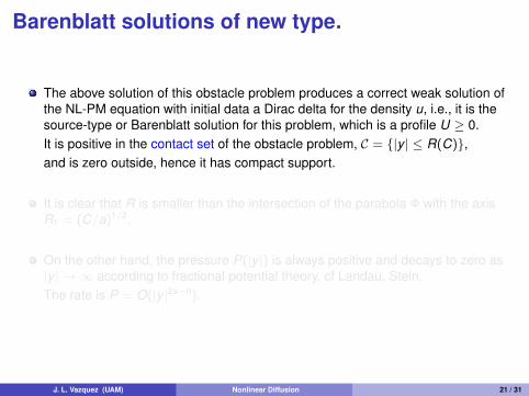
Barenblatt solutions of new type.
The above solution of this obstacle problem produces a correct weak solution ofthe NL-PM equation with initial data a Dirac delta for the density u, i.e., it is thesource-type or Barenblatt solution for this problem, which is a profile U ≥ 0.It is positive in the contact set of the obstacle problem, C = |y | ≤ R(C),and is zero outside, hence it has compact support.
It is clear that R is smaller than the intersection of the parabola Φ with the axisR1 = (C/a)1/2.
On the other hand, the pressure P(|y |) is always positive and decays to zero as|y | → ∞ according to fractional potential theory, cf Landau, Stein.The rate is P = O(|y |2s−n).
J. L. Vazquez (UAM) Nonlinear Diffusion 21 / 31
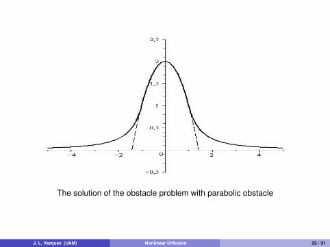
The solution of the obstacle problem with parabolic obstacle
J. L. Vazquez (UAM) Nonlinear Diffusion 22 / 31

Estimates for the renormalized problem.Entropy dissipation.
Our main problem is now to prove that these profiles are attractors for therenormalized flow.
We review the estimates of Main Estimates Section above in order to adapt themto the renormalized problem.
There is no problem is reproving mass conservation or positivity.
First energy estimate becomes (recall that H = K 1/2)
(8)
ddτ
∫v(y , τ) log v(y , τ) dy
= −∫|∇Hv |2 dy − β
∫∇v · y
= −∫|∇Hv |2 dy + α
∫v .
J. L. Vazquez (UAM) Nonlinear Diffusion 23 / 31

Estimates for the renormalized problem. Entropydissipation.
However, the second energy estimate has an essential change. We need todefine the entropy of the renormalized flow as
(9) E(v(τ)) :=12
∫Rn
(v K (v) + βy2v) dy
The entropy contains two terms. The first is
E1(v(τ)) :=
∫Rn
v K (v) dy =
∫Rn|Hv |2 dy , H = K 1/2
hence positive. The second is the moment E2(v(τ)) = M2(v(τ)) :=∫
y2v dy ,also positive. By differentiation we get
(10)d
dτE(v) = −I(v), I(v) :=
∫ ∣∣∣∣∇(Kv +β
2y2)
∣∣∣∣2 vdy .
This means that whenever the initial entropy is finite, then E(v(τ)) is uniformlybounded for all τ > 0, I(v) is integrable in (0,∞) and
E(v(τ)) +
∫∫ ∣∣∣∣∇(Kv +β
2y2)
∣∣∣∣2 vdy dt ≤ E(v0).
J. L. Vazquez (UAM) Nonlinear Diffusion 24 / 31
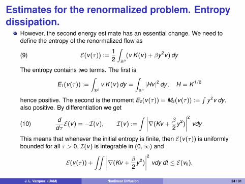
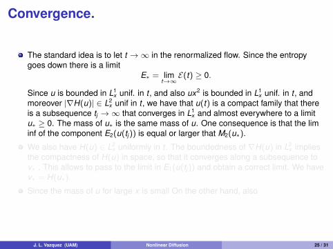
Convergence.
The standard idea is to let t →∞ in the renormalized flow. Since the entropygoes down there is a limit
E∗ = limt→∞E(t) ≥ 0.
Since u is bounded in L1x unif. in t , and also ux2 is bounded in L1
x unif. in t , andmoreover |∇H(u)| ∈ L2
x unif in t , we have that u(t) is a compact family that thereis a subsequence tj →∞ that converges in L1
x and almost everywhere to a limitu∗ ≥ 0. The mass of u∗ is the same mass of u. One consequence is that the liminf of the component E2(u(tj )) is equal or larger that M2(u∗).
We also have H(u) ∈ L2x uniformly in t . The boundedness of ∇H(u) in L2
x impliesthe compactness of H(u) in space, so that it converges along a subsequence tov∗ . This allows to pass to the limit in E1(u(tj )) and obtain a correct limit. We havev∗ = H(u∗).
Since the mass of u for large x is small On the other hand, also
J. L. Vazquez (UAM) Nonlinear Diffusion 25 / 31
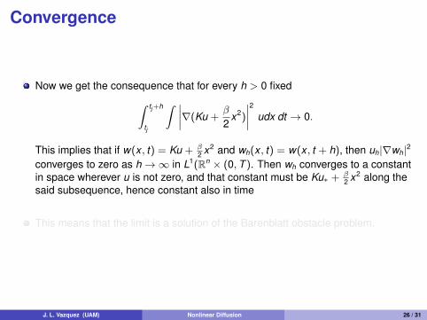
Convergence
Now we get the consequence that for every h > 0 fixed∫ tj+h
tj
∫ ∣∣∣∣∇(Ku +β
2x2)
∣∣∣∣2 udx dt → 0.
This implies that if w(x , t) = Ku + β2 x2 and wh(x , t) = w(x , t + h), then uh|∇wh|2
converges to zero as h→∞ in L1(Rn × (0,T ). Then wh converges to a constantin space wherever u is not zero, and that constant must be Ku∗ + β
2 x2 along thesaid subsequence, hence constant also in time
This means that the limit is a solution of the Barenblatt obstacle problem.
J. L. Vazquez (UAM) Nonlinear Diffusion 26 / 31

Recent workBiler, Imbert and Karch. In a note just submitted to CRAS (Barenblatt profiles fora nonlocal porous medium equation) the authors study the more general equation
ut = ∇ · (uΛα−1um), 0 < α < 2
and obtain our type of Barenblatt solutions for every m > 1 with a very nice addedinformation, they happen to be explicit of the form
u(x , t) = Ct−µ(R2 − x2t−2ν))α/2(m−1)+
it uses an important identity by Getoor, (−∆)α/2(1− y2)α/2+ = K , valid inside the
support. Observe the boundary behavior.
The work with Serfaty (Barcelona 2012, published 2014) shows that the limits → 1 of the solutions of the fractional diffusion problem produces the solutions ofthe hydrodynamic limit
ut = ∇ · (u∇p), −∆p = u .
This happens in all dimensions n ≥ 2. The corresponding self-similar solutionstake the form
U(x , t) = t−1H(x/t1/n)
and H is the characteristic function of a ball BR(0). This means in Physics anexpanding vortex patch. This type of solutions is NOT continuous.
J. L. Vazquez (UAM) Nonlinear Diffusion 27 / 31
Our first project. Last resultsLimit s → 1 S. Serfaty, and J. L. Vazquez, Hydrodynamic Limit of Nonlinear.Diffusion with Fractional Laplacian Operators, Calc. Var. PDEs 526, online;arXiv:1205.6322v1 [math.AP], may 2012.
A presentation of this topic and results for the Proceedings from the AbelSymposium 2010.
J. L. Vazquez. Nonlinear Diffusion with Fractional Laplacian Operators. in“Nonlinear partial differential equations: the Abel Symposium 2010”, Holden,Helge & Karlsen, Kenneth H. eds., Springer, 2012. Pp. 271–298.
Proving that the self-similar solutions of Barenblatt type (Caffareli-Vazquez,Biler-Karch-Monneau) are attractors with calculated rate in 1D.
Exponential Convergence Towards Stationary States for the 1D Porous MediumEquation with Fractional Pressure, by J. A. Carrillo, Y. Huang, M. C. Santos, andJ. L. Vazquez. JDE, 2015.Uses entropy analysis and Bakry Emery method. Problem is open (and quiteinteresting in higher dimensions). Previous work by Biler, Karch and Monneau in1D with no rate.
See JLV’s webpage, preprints, arxiv.
J. L. Vazquez (UAM) Nonlinear Diffusion 28 / 31

Work to Do
Study the regularity of the solutions
Study the equation and regularity of the free boundary
Study fine asymptotic behavior, and extend to other classes of data
Study these nonlocal problems in bounded domains
Decide conditions of uniqueness
Decide conditions of comparison
Write a performing numerical code
Consider different nonlocal nonlinear diffusion problems
Discuss the Stochastic Particle Models in the literature that involve long-rangeeffects and anomalous diffusion parameters.
J. L. Vazquez (UAM) Nonlinear Diffusion 29 / 31

There is much more going on,but let us stop here.
End
Thank you♠ ♠ ♠
Gracias
J. L. Vazquez (UAM) Nonlinear Diffusion 30 / 31

There is much more going on,but let us stop here.
End
Thank you♠ ♠ ♠
Gracias
J. L. Vazquez (UAM) Nonlinear Diffusion 30 / 31

There is much more going on,but let us stop here.
End
Thank you♠ ♠ ♠
Gracias
J. L. Vazquez (UAM) Nonlinear Diffusion 30 / 31
There is much more going on,but let us stop here.
End
Thank you♠ ♠ ♠
Gracias
J. L. Vazquez (UAM) Nonlinear Diffusion 30 / 31
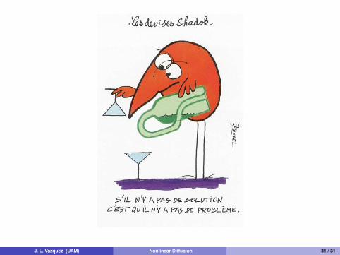
J. L. Vazquez (UAM) Nonlinear Diffusion 31 / 31

1
The theory of nonlinear diffusionwith fractional operators II
JUAN LUIS VAZQUEZ
Departamento de MatematicasUniversidad Autonoma de Madridand Royal Academy of Sciences
CIME Summer Course“Nonlocal and Nonlinear Diffusions and
Interactions: New Methods and Directions”
Cetraro, Italia July 7, 2016

2
Outline
1 The second model of fractional diffusion: FPME
2 Recent team work
3 Operators and Equations in Bounded Domains
3
Outline
1 The second model of fractional diffusion: FPME
2 Recent team work
3 Operators and Equations in Bounded Domains

Outline
1 The second model of fractional diffusion: FPME
2 Recent team work
3 Operators and Equations in Bounded Domains
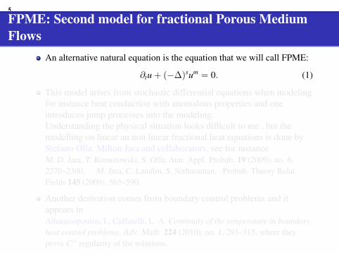
5
FPME: Second model for fractional Porous MediumFlows
An alternative natural equation is the equation that we will call FPME:
∂tu + (−∆)sum = 0. (1)
This model arises from stochastic differential equations when modelingfor instance heat conduction with anomalous properties and oneintroduces jump processes into the modeling.Understanding the physical situation looks difficult to me , but themodelling on linear an non linear fractional heat equations is done byStefano Olla, Milton Jara and collaborators, see for instanceM. D. Jara, T. Komorowski, S. Olla, Ann. Appl. Probab. 19 (2009), no. 6,2270–2300. M. Jara, C. Landim, S. Sethuraman, Probab. Theory Relat.Fields 145 (2009), 565–590.
Another derivation comes from boundary control problems and itappears inAthanasopoulos, I.; Caffarelli, L. A. Continuity of the temperature in boundaryheat control problems, Adv. Math. 224 (2010), no. 1, 293–315, where theyprove Cα regularity of the solutions.

6
Mathematical theory of the Fractional Heat Equation
The Linear Problem isut + (−∆)s(u) = 0
We take x ∈ Rn, 0 < m <∞, 0 < s < 1, with initial data in u0 ∈ L1(Rn).Normally, u0, u ≥ 0.This model represents the linear flow generated by the so-called Levy processesin Stochastic PDEs, where the transition from one site xj of the mesh to anothersite xk has a probability that depends on the distance |xk − xj| in the form of aninverse power for j 6= k. The power we take is c |xk − xj|−n−2s. The range is0 < s < 1. The limit from random walk to the continuous equation is done byE. Valdinoci, in From the long jump random walk to the fractional Laplacian,Bol. Soc. Esp. Mat. Apl. 49 (2009), 33-44.The solution of the linear equation can be obtained in Rn by means ofconvolution with the fractional heat kernel
u(x, t) =
∫u0(y)Pt(x− y) dy,
and people in probability (like Blumental and Getoor) proved in the 1960s that
Pt(x) t(t1/s + |x|2
)(n+2s)/2 ⇒ look at the fat tail.

7
The paperB. Barrios, I. Peral, F. Soria, E. Valdinoci. “A Widder’s type theorem for theheat equation with nonlocal diffusion” Arch. Ration. Mech. Anal. 213 (2014),no. 2, 629-650, studies the theory in classes of (maybe) large functions andstudies the question: is every solution representable by the convolution formula.The answer is yes if the solutions are ‘nice’ strong solutions and the growth in xis no more that u(x, t) ≤ (1 + |x|)a with a < 2s.
Our recent paperM. Bonforte, Y. Sire, J. L. Vazquez. “Optimal Existence and UniquenessTheory for the Fractional Heat Equation”, Arxiv:1606.00873v1solves the problem of existence and uniqueness of solutions when the initialdata is a locally finite Radon measure with the condition∫
Rn(1 + |x|)−(n+2s) dµ(x) <∞ . (2)
Moreover we prove that any constructed solution by convolution, or any veryweak solution u ≥ 0, has an initial trace µ which is a measure in the above classMs. So the result closes the problem of the Widder theory for the fractionalheat equation posed in Rn.
The paper goes on to tell what you want to know about this semigroup fornonnegative solutions. Arxiv is free.

8
Recent coauthors
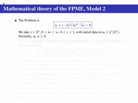
9
Mathematical theory of the FPME, Model 2
The Problem isut + (−∆)s(|u|m−1u) = 0
We take x ∈ Rn, 0 < m <∞, 0 < s < 1, with initial data in u0 ∈ L1(Rn).Normally, u0, u ≥ 0.This second model, M2 here, represents another type of nonlinear interpolation,this time between
ut −∆(|u|m−1u) = 0 and ut + |u|m−1u = 0
A complete analysis of the Cauchy problem done byA. de Pablo, F. Quiros, Ana Rodrıguez, and J.L.V., in 2 papers appeared inAdvances in Mathematics (2011) and Comm. Pure Appl. Math. (2012).In the classical Benilan-Brezis-Crandall style, a semigroup of weak energysolutions is constructed, the L1 − L∞ smoothing effect works,Cα regularity (if m is not near 0),Nonnegative solutions have infinite speed of propagation for all m and s⇒ nocompact support. But Model 1 with Caffarelli did have the compact supportproperty.

10
Outline
1 The second model of fractional diffusion: FPME
2 Recent team work
3 Operators and Equations in Bounded Domains

11
Outline of work done for model M2Comparison of models M1 and M2 is quite interesting
Existence of self-similar solutions, paper JLV, JEMS 2014. The fractionalBarenblatt solution is constructed:
U(x, t) = t−αF(xt−β)
The difficulty is to find F as the solution of an elliptic nonlinear equation offractional type.F has behaviour like a Blumental tail F(r) ∼ r−(n+2s for m ≥ 1, but not forsome fast diffusion m < 1. Asymptotic behaviour follows: the Barenblattsolution is an attractor.
A priori upper and lower estimates of intrinsic, local type. Paper with MatteoBonforte in Advances Math., 2014 for problems posed in Rn.- Quantitative positivity and Harnack Inequalities follow.Against some prejudice due to the nonlocal character of the diffusion, we areable to obtain them here for fractional PME/FDE using a technique of weightedintegrals to control the tails of the integrals in a uniform way. The novelty is theweighted functional inequalities.Work on bounded domains is more recent and very interesting.
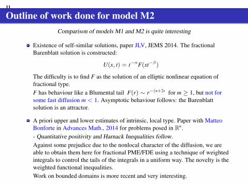

12
Existence of classical solutions and higher regularity for the FPME andthe more general model
∂tu + (−∆)sΦ(u) = 0
Two works by group PQRV. The first appeared at J. Math. Pures Appl.treats the model case Φ(u) = log(1 + u), which is interesting. Secondis general Φ and is accepted 2015 in J. Eur. Math. Soc. It proves higherregularity for nonnegative solutions of this fractional porous mediumequation.Recent extension of C∞ regularity to solutions in bounded domains byM. Bonforte, A. Figalli, X. Ros-Oton, Infinite speed of propagation andregularity of solutions to the fractional porous medium equation ingeneral domains, arxiv1510.03758.
Symmetrization (Schwarz and Steiner). Collaboration with BrunoVolzone, two papers at JMPA. Applying usual symmetrizationtechniques is not easy and we have many open problems. Recentcollaboration with Sire and Volzone on the Faber Krahn inequality.
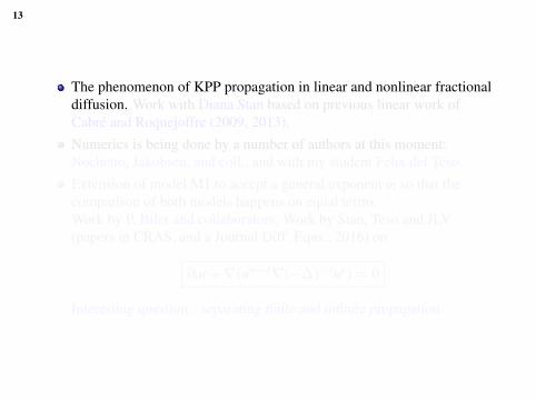
13
The phenomenon of KPP propagation in linear and nonlinear fractionaldiffusion. Work with Diana Stan based on previous linear work ofCabre and Roquejoffre (2009, 2013).Numerics is being done by a number of authors at this moment:Nochetto, Jakobsen, and coll., and with my student Felix del Teso.Extension of model M1 to accept a general exponent m so that thecomparison of both models happens on equal terms.Work by P. Biler and collaborators. Work by Stan, Teso and JLV(papers in CRAS, and a Journal Diff. Eqns., 2016) on
∂tu +∇(um−1∇(−∆)−sup) = 0
Interesting question : separating finite and infinite propagation.
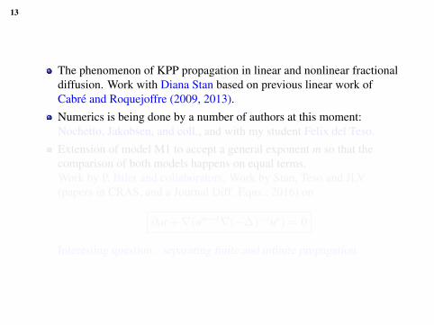
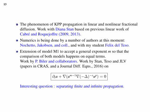

14
Younger collaborators

15
A detailed account on such progress is obtained in the papers (cf. arxiv)and in the following reference that is meant as a survey for two-yearprogress on Model M2
Recent progress in the theory of Nonlinear Diffusion with FractionalLaplacian Operators, by Juan Luis Vazquez. In “Nonlinear elliptic andparabolic differential equations”, Disc. Cont. Dyn. Syst. - S 7, no. 4(2014), 857–885.
Fast diffusion and extinction. Very singular fast diffusion. Paper withBonforte and Segatti in CalcVar. 2016, on non-existence due toinstantaneous extinction.
fractional p-Laplacian flows This is a rather new topic. The definitionof the nonlocal p-laplacian operator was given in Mingione’s last talk asthe Euler-Lagrange operator corresponding to a power-like functionalwith nonlocal kernel of the s-Laplacian type. There the aim is elliptictheory. Paper by JLV, 2015 in arXiv, appeared JDE 2016, solvesparabolic theory on bounded domains.
Very degenerate nonlinearities, like the Mesa Problem. This is the limitof NLPME with m→∞. Paper by JLV, Interfaces Free Bound. 2015.

16
Some future Directions
Other nonlocal linear operators (hot topic)
Elliptic theory (main topic, by many authors)
Geostrophic flows (this is more related to Fluid Mechanics)
Reaction-diffusion and blowup
Geometrical flows, fractional Yamabe (MMar Gonzalez, Sire)
Chemotaxis systems, ....

16
Some future Directions
Other nonlocal linear operators (hot topic)
Elliptic theory (main topic, by many authors)
Geostrophic flows (this is more related to Fluid Mechanics)
Reaction-diffusion and blowup
Geometrical flows, fractional Yamabe (MMar Gonzalez, Sire)
Chemotaxis systems, ....
17
Outline
1 The second model of fractional diffusion: FPME
2 Recent team work
3 Operators and Equations in Bounded Domains

18
Operators and Equations in Bounded Domains
Work needs a different lecture. It comes from long time collaborationwith Matteo Bonforte, and recently with Yannick Sire and AlessioFigalli.We develop a new programme for Existence, Uniqueness, Positivity, Apriori bounds and Asymptotic behaviour for fractional porous mediumequations on bounded domains, after examining very carefully the setof suitable concepts of FLO in a bounded domain.But the main issue is how many natural definitions we find of the FLOin a bounded domain.Then we use the “dual” formulation of the problem and the concept ofweak dual solution. In brief, we use the linearity of the operator L to liftthe problem to a problem for the potential function
U(x, t) =
∫Ω
u(y, t)G(x, y)dy
Where G is the elliptic Green function for L.

19
Fractional Laplacian operators on bounded domainsThe Restricted Fractional Laplacian operator (RFL) is defined via thehypersingular kernel in Rn, “restricted” to functions that are zero outside Ω.
(−∆|Ω)sg(x) = cN,s P.V.∫RN
g(x)− g(z)|x− z|n+2s dz , with supp(g) ⊂ Ω .
where s ∈ (0, 1) and cn,s > 0 is a normalization constant.
(−∆|Ω)s is a self-adjoint operator on L2(Ω) with a discrete spectrum:
EIGENVALUES: 0 < λ1 ≤ λ2 ≤ . . . ≤ λj ≤ λj+1 ≤ . . . and λj j2s/N .
EIGENFUNCTIONS: φj are the normalized eigenfunctions, are only Holdercontinuous up to the boundary, namely φj ∈ Cs(Ω) .Lateral boundary conditions for the RFL:
u(t, x) = 0 , in (0,∞)×(RN \ Ω
).
The Green function G of RFL satisfies a strong behaviour condition (K4)
G(x, y) 1|x− y|N−2s
(δγ(x)
|x− y|γ ∧ 1)(
δγ(y)
|x− y|γ ∧ 1), with γ = s
References.(K4) Bounds proven by Bogdan, Grzywny, Jakubowski, Kulczycki,Ryznar (1997-2010). Eigenvalues: Blumental-Getoor (1959), Chen-Song(2005).

20
Fractional Laplacian operators on bounded domains
The The Spectral Fractional Laplacian operator (SFL)
(−∆Ω)sg(x) =∞∑j=1
λsj gj φj(x) =
1Γ(−s)
∫ ∞0
(et∆Ωg(x)− g(x)
) dtt1+s .
where ∆Ω is the classical Dirichlet Laplacian on the domain Ω,
gj =
∫Ω
g(x)φj(x) dx , with ‖φj‖L2(Ω) = 1 .
EIGENVALUES: 0 < λ1 ≤ λ2 ≤ . . . ≤ λj ≤ λj+1 ≤ . . . and λj j2/n.
EIGENFUNCTIONS: φj are as smooth as the boundary of Ω allows,namely when ∂Ω is Ck, then φj ∈ C∞(Ω) ∩ Ck(Ω) for all k ∈ N .
Lateral boundary conditions for the SFL. They are better defined by using theCaffarelli-Silvestre extension adapted to bounded domain as a cylinder. Thenwe put U = 0 on the lateral boundary x ∈ ∂Ω, y > 0.
The Green function of SFL satisfies a stronger assumption
G(x, y) 1|x− y|n−2s
(δγ(x)
|x− y|γ ∧ 1)(
δγ
|x− y|γ ∧ 1), with γ = 1
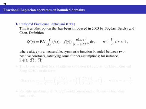
21
Fractional Laplacian operators on bounded domains
Censored Fractional Laplacians (CFL)This is another option that has been introduced in 2003 by Bogdan, Burdzy andChen. Definition
Lf (x) = P.V.∫
Ω
(f (x)− f (y))a(x, y)
|x− y|N+2s dy , with12< s < 1 ,
where a(x, y) is a measurable, symmetric function bounded between twopositive constants, satisfying some further assumptions; for instancea ∈ C1(Ω× Ω).
The Green function G(x, y) satisfies condition K4 , proven by Chen, Kim andSong (2010), in the form
G(x, y) 1|x− y|N−2s
(δγ(x)
|x− y|γ ∧ 1)(
δγ(y))
|x− y|γ ∧ 1), with γ = s− 1
2.
Roughly speaking, s ∈ (0, 1/2] would correspond to Neumann boundaryconditions.

22
We have presented 3 models of Dirichlet fractional Laplacian.Put
[a(x, y) = const
]in the last case. The estimates (K4) show that
they are of course not equivalent.
References. K. Bogdan, K. Burdzy, K., Z.-Q. Chen. Censored stableprocesses. Probab. Theory Relat. Fields (2003).Z.-Q. Chen, P. Kim, R. Song, Two-sided heat kernel estimates forcensored stable-like processes. Probab. Theory Relat. Fields (2010).
There is a crowd of generalizations. See papers or recent talks by M.Bonforte.
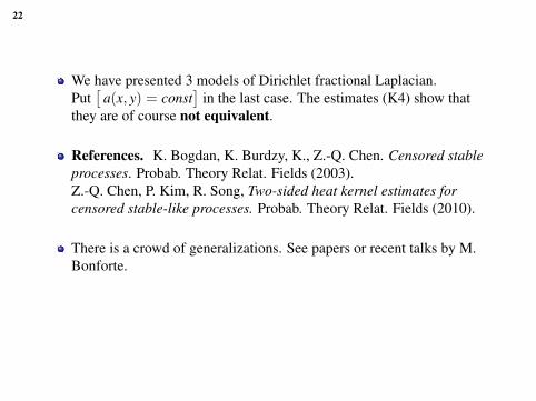
23
But let us stop here
and wish you a happy summer.
Thank you, Gracias, Grazie
23
But let us stop here
and wish you a happy summer.
Thank you, Gracias, Grazie

23
But let us stop here
and wish you a happy summer.
Thank you, Gracias, Grazie

23
But let us stop here
and wish you a happy summer.
Thank you, Gracias, Grazie