Embed Size (px)
Citation preview

NonlinearControl
3rd ElgersburgSchool 2011
Nonlinear Control3rd Elgersburg School 2011
Randy Freeman
Professor
Department of Electrical Engineering & Computer Science

NonlinearControl
3rd ElgersburgSchool 2011 Acknowledgments
Many thanks to the following:
Organizers:Achim IlchmannTimo ReisFabian Wirth
Sponsor:
Exercises and discussions by Dr. Robert Gregg

NonlinearControl
3rd ElgersburgSchool 2011 Linear control of nonlinear systems
First pass at controlling a nonlinear system:linearize the dynamics about an operating point,or use system identification to fit a linear model
use the linear model to design a linear controller
treat any nonlinearities as model uncertainty,to be handled with linear robust or adaptive control
This is not what this short course is about.

NonlinearControl
3rd ElgersburgSchool 2011 What is nonlinear control?
Nonlinear controlNonlinear control means design and analysis using nonlinearmodels for the plant and/or the controller.
Why nonlinear control?linear models might not capture the relevant behaviorlinear models might be valid only for small signalsnonlinear is more fun than linear!

NonlinearControl
3rd ElgersburgSchool 2011 Goals of this short course
to make you familiar with some of the fundamentalconcepts in nonlinear control
to give you some tools to allow you to try some basicnonlinear controller designs
to give you a starting point for further exploration
Not a comprehensive reviewThis is not a survey course, and we will only cover selectedtopics (some in more depth than others).
Focus of the courseThe focus will be on the mathematical theory and design andanalysis tools, not on practical implementation issues.

NonlinearControl
Nonlinearmodels
Nonlineardifferentialequations
Stability ofequilibria
Stability ofinvariant sets
Stability fortime-varyingsystems
Stability forsystems withinputs
3rd ElgersburgSchool 2011
Part I
Nonlinear models and stability

NonlinearControl
Nonlinearmodels
Nonlineardifferentialequations
Stability ofequilibria
Stability ofinvariant sets
Stability fortime-varyingsystems
Stability forsystems withinputs
3rd ElgersburgSchool 2011 Outline
1 Nonlinear models
2 Nonlinear differential equations
3 Stability of equilibria
4 Stability of invariant sets
5 Stability for time-varying systems
6 Stability for systems with inputs

NonlinearControl
Nonlinearmodels
Nonlineardifferentialequations
Stability ofequilibria
Stability ofinvariant sets
Stability fortime-varyingsystems
Stability forsystems withinputs
3rd ElgersburgSchool 2011 Linear models in continuous time
State-space models with state 𝑥(𝑡), input 𝑢(𝑡), and output 𝑦(𝑡):
Time-varying
��(𝑡) = 𝐴(𝑡)𝑥(𝑡) + 𝐵(𝑡)𝑢(𝑡)𝑦(𝑡) = 𝐶(𝑡)𝑥(𝑡) + 𝐷(𝑡)𝑢(𝑡)
Time-invariant
��(𝑡) = 𝐴𝑥(𝑡) + 𝐵𝑢(𝑡)𝑦(𝑡) = 𝐶𝑥(𝑡) + 𝐷𝑢(𝑡)
Input/output models:
Time domain
𝑦(𝑡) = ∫∞
−∞ℎ(𝑡 − 𝜏)𝑢(𝜏) 𝑑𝜏
Frequency domain
𝑌(𝑠) = 𝐻(𝑠)𝑈(𝑠)
Others: operator models, behavioral models, …

NonlinearControl
Nonlinearmodels
Nonlineardifferentialequations
Stability ofequilibria
Stability ofinvariant sets
Stability fortime-varyingsystems
Stability forsystems withinputs
3rd ElgersburgSchool 2011 Continuous-time state-space models
Nonlinear ordinary-differential-equation models:
Time-varying
�� = 𝑓(𝑡, 𝑥, 𝑢)𝑦 = ℎ(𝑡, 𝑥, 𝑢)
Time-invariant
�� = 𝑓(𝑥, 𝑢)𝑦 = ℎ(𝑥, 𝑢)
Control-affine time-varying
�� = 𝑓(𝑡, 𝑥) + 𝑔(𝑡, 𝑥)𝑢𝑦 = ℎ(𝑡, 𝑥) + 𝑗(𝑡, 𝑥)𝑢
Control-affine time-invariant
�� = 𝑓(𝑥) + 𝑔(𝑥)𝑢𝑦 = ℎ(𝑥) + 𝑗(𝑥)𝑢
ℝ𝑛 = vector space of 𝑛-tuples of real numbersstate 𝑥 ∈ 𝑋, where 𝑋 is an open subset of ℝ𝑛,or 𝑋 is a differentiable manifold of dimension 𝑛input 𝑢 ∈ ℝ𝑚, output 𝑦 ∈ ℝ𝑝

NonlinearControl
Nonlinearmodels
Nonlineardifferentialequations
Stability ofequilibria
Stability ofinvariant sets
Stability fortime-varyingsystems
Stability forsystems withinputs
3rd ElgersburgSchool 2011 Example: simple pendulum
𝜃
𝑢
ℓ
𝑚
𝑚 = mass of end weightℓ = length of rod𝑔 = acceleration due to gravity𝑏 = damping coefficient𝑢 = input torque
Equations of motion:
𝑚ℓ2 + 𝑏 + 𝑚𝑔ℓ sin( ) = 𝑢
Choose state coordinates 𝑥1 = , 𝑥2 =
��1 = 𝑥2
��2 = −𝑔ℓ
sin(𝑥1) − 𝑏𝑚ℓ2 𝑥2 + 1
𝑚ℓ2 𝑢

NonlinearControl
Nonlinearmodels
Nonlineardifferentialequations
Stability ofequilibria
Stability ofinvariant sets
Stability fortime-varyingsystems
Stability forsystems withinputs
3rd ElgersburgSchool 2011 Linearization about a trajectory
Given: a specific trajectory (��(𝑡), 𝑢(𝑡), 𝑦(𝑡)) with��(𝑡) = 𝑓(𝑡, ��(𝑡), 𝑢(𝑡))𝑦(𝑡) = ℎ(𝑡, ��(𝑡), 𝑢(𝑡))
Define: error variables
𝛿𝑥(𝑡) = 𝑥(𝑡) − ��(𝑡) , 𝛿𝑢(𝑡) = 𝑢(𝑡) − 𝑢(𝑡) , 𝛿𝑦(𝑡) = 𝑦(𝑡) − 𝑦(𝑡)
Compute: linear approximation from Jacobian matrices
𝛿��(𝑡) ≈ [𝜕𝑓𝜕𝑥(𝑡, ��(𝑡), 𝑢(𝑡))]𝛿𝑥(𝑡) + [
𝜕𝑓𝜕𝑢 (𝑡, ��(𝑡), 𝑢(𝑡))]𝛿𝑢(𝑡)
𝛿𝑦(𝑡) ≈ [𝜕ℎ𝜕𝑥(𝑡, ��(𝑡), 𝑢(𝑡))]𝛿𝑥(𝑡) + [
𝜕ℎ𝜕𝑢 (𝑡, ��(𝑡), 𝑢(𝑡))]𝛿𝑢(𝑡)

NonlinearControl
Nonlinearmodels
Nonlineardifferentialequations
Stability ofequilibria
Stability ofinvariant sets
Stability fortime-varyingsystems
Stability forsystems withinputs
3rd ElgersburgSchool 2011
Linearization about an equilibriumSimple pendulum example
An equilibrium is a constant trajectory (��, 𝑢, 𝑦), and it satisfies0 = 𝑓(𝑡, ��, 𝑢) and 𝑦 = ℎ(𝑡, ��, 𝑢) for all 𝑡.
Equilibrium trajectory with 𝑢 = 𝑚𝑔ℓ sin(��1) and ��2 = 0:
𝛿�� ≈ ⎡⎢⎣
0 1
− 𝑔ℓ cos(��1) − 𝑏
𝑚ℓ2
⎤⎥⎦
𝛿𝑥 + ⎡⎢⎣
01
𝑚ℓ2
⎤⎥⎦
𝛿𝑢
This LTI system iscontrollablestable when the equilibrium angle ��1 is in the bottom halfof the circle, that is, when |��1| < 𝜋
2unstable when ��1 is in the top half of the circle

NonlinearControl
Nonlinearmodels
Nonlineardifferentialequations
Stability ofequilibria
Stability ofinvariant sets
Stability fortime-varyingsystems
Stability forsystems withinputs
3rd ElgersburgSchool 2011 Notation and terminology for classes of functions
A mapping 𝑓 ∶ 𝑈 → 𝑈′, where 𝑈 ⊂ ℝ𝑛 and 𝑈′ ⊂ ℝ𝑚, is called
C0 when it is continuous
a homeomorphism when it is C0 and has a C0 inverse
C𝑟 when 𝑈 is open and 𝑓 is 𝑟 times continuouslydifferentiable (𝑟 ⩾ 1, including 𝑟 = ∞)
a C𝑟-diffeomorphism when it is C𝑟 and has a C𝑟 inverse(in this case 𝑈′ is open and 𝑛 = 𝑚)
a diffeomorphism when it is a C∞-diffeomorphism
Inverse function theoremIf 𝑓 is C𝑟 near 𝑥 ∈ 𝑈 and if its Jacobian matrix is nonsingularat 𝑥, then 𝑓 is a C𝑟-diffeomorphism near 𝑥.

NonlinearControl
Nonlinearmodels
Nonlineardifferentialequations
Stability ofequilibria
Stability ofinvariant sets
Stability fortime-varyingsystems
Stability forsystems withinputs
3rd ElgersburgSchool 2011 Lipschitz continuous functions
DefinitionA mapping 𝑓 ∶ 𝑈 → 𝑈′ is Lipschitz continuous when thereexists 𝐿 ⩾ 0 such that
|𝑓(𝑥1) − 𝑓(𝑥2)| ⩽ 𝐿|𝑥1 − 𝑥2| for all 𝑥1, 𝑥2 ∈ 𝑈 .
It is locally Lipschitz continuous when it is Lipschitzcontinuous on a neighborhood of every point in 𝑈.
Lipschitz continuous⇓
C1 ⟹ locally Lipschitz continuous ⟹ C0
Examples for 𝑓 ∶ ℝ → ℝ:𝑓(𝑥) = |sin(𝑥)| is Lipschitz continuous but not C1
𝑓(𝑥) = 𝑥2 is locally Lipschitz but not Lipschitz𝑓(𝑥) = √|𝑥| is C0 but not locally Lipschitz

NonlinearControl
Nonlinearmodels
Nonlineardifferentialequations
Stability ofequilibria
Stability ofinvariant sets
Stability fortime-varyingsystems
Stability forsystems withinputs
3rd ElgersburgSchool 2011 Coordinates: labeling the states
Local and global Cartesian coordinatesA homeomorphism from an open subset of the state space 𝑋to an open subset of ℝ𝑛 describes a local coordinate systemin which the elements of the vector in ℝ𝑛 are the 𝑛 coordinatesof the corresponding state.A coordinate mapping whose domain is the entire space 𝑋describes a global coordinate system.
Change of coordinatesIf the domains of two local coordinate systems overlap, thenthere is a homeomorphism from one set of coordinates to theother (defined on the overlapping region).The two coordinate systems are called compatible when thismapping is a diffeomorphism.
NonlinearControl
Nonlinearmodels
Nonlineardifferentialequations
Stability ofequilibria
Stability ofinvariant sets
Stability fortime-varyingsystems
Stability forsystems withinputs
3rd ElgersburgSchool 2011
Coordinates: labeling the statesSimple pendulum example
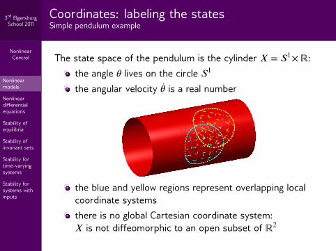
The state space of the pendulum is the cylinder 𝑋 = 𝑆1× ℝ:the angle lives on the circle 𝑆1
the angular velocity is a real number
the blue and yellow regions represent overlapping localcoordinate systemsthere is no global Cartesian coordinate system:𝑋 is not diffeomorphic to an open subset of ℝ2

NonlinearControl
Nonlinearmodels
Nonlineardifferentialequations
Stability ofequilibria
Stability ofinvariant sets
Stability fortime-varyingsystems
Stability forsystems withinputs
3rd ElgersburgSchool 2011
Coordinates: labeling the statesSome coordinates may be more convenient than others
Nonlinear system with 𝑋 = ℝ2 and 𝑥 = (𝑥1, 𝑥2):
��1 = 𝑥2 − 𝑥21
��2 = 𝑥1 + 2𝑥1(𝑥2 − 𝑥21) + 𝑢
Consider the diffeomorphism Φ ∶ 𝑋 → 𝑋 given by
𝑧 =[𝑧1𝑧2]= Φ(𝑥) =[
𝑥1𝑥2 − 𝑥2
1] , 𝑥 =[𝑥1𝑥2]= Φ−1(𝑧) =[
𝑧1𝑧2
1 + 𝑧2]
Same system in new coordinates 𝑧 = (𝑧1, 𝑧2):
𝑧1 = 𝑧2
𝑧2 = 𝑧1 + 𝑢
The system is linear when written in the new coordinates!

NonlinearControl
Nonlinearmodels
Nonlineardifferentialequations
Stability ofequilibria
Stability ofinvariant sets
Stability fortime-varyingsystems
Stability forsystems withinputs
3rd ElgersburgSchool 2011 Outline
1 Nonlinear models
2 Nonlinear differential equations
3 Stability of equilibria
4 Stability of invariant sets
5 Stability for time-varying systems
6 Stability for systems with inputs

NonlinearControl
Nonlinearmodels
Nonlineardifferentialequations
Stability ofequilibria
Stability ofinvariant sets
Stability fortime-varyingsystems
Stability forsystems withinputs
3rd ElgersburgSchool 2011
Solutions to ordinary differential equationsTime-invariant case
System with no input, or with some fixed feedback 𝑢 = 𝑢(𝑥):
𝑓(𝑥) is a vector field defined on 𝑋:
�� = 𝑓(𝑥) (*)
A solution of (*) from an initial condition 𝑥0 ∈ 𝑋 is a function𝑥(𝑡) defined on an open interval ℐ(𝑥0) ⊂ ℝ such that
0 ∈ ℐ(𝑥0) and 𝑥(0) = 𝑥0
𝑥(𝑡) is C1 on ℐ(𝑥0) with ��(𝑡) = 𝑓(𝑥(𝑡)) for all 𝑡 ∈ ℐ(𝑥0)
ℐ(𝑥0) is the maximal interval of existence: there is noother solution defined on a larger open interval whichagrees with 𝑥(𝑡) on ℐ(𝑥0)

NonlinearControl
Nonlinearmodels
Nonlineardifferentialequations
Stability ofequilibria
Stability ofinvariant sets
Stability fortime-varyingsystems
Stability forsystems withinputs
3rd ElgersburgSchool 2011
Existence and uniqueness of solutionsTime-invariant case
Sufficient conditions for local existence and uniqueness:
𝑓(𝑥) is continuous on 𝑋 ⟹ solutions exist ∀𝑥0
𝑓(𝑥) is locally Lipschitz on 𝑋 ⟹ solutions are unique
Global existence: a locally Lipschitz vector field 𝑓(𝑥) is calledcomplete when ℐ(𝑥0) = ℝ for all 𝑥0 ∈ 𝑋forward-complete when sup ℐ(𝑥0) = ∞ for all 𝑥0 ∈ 𝑋
Sufficient conditions for completeness (locally Lipschitz 𝑓):∗∗ 𝑓(𝑥) is Lipschitz on 𝑋 = ℝ𝑛 ⟹ 𝑓(𝑥) is complete
𝑋 is a compact manifold ⟹ 𝑓(𝑥) is complete
∗∗ this property depends on the choice of coordinates!

NonlinearControl
Nonlinearmodels
Nonlineardifferentialequations
Stability ofequilibria
Stability ofinvariant sets
Stability fortime-varyingsystems
Stability forsystems withinputs
3rd ElgersburgSchool 2011 Example: non-uniqueness of solutions
𝑓 is C0 but not locally Lipschitz continuous:
�� = 2√|𝑥| 𝑥(0) = 0 𝑋 = ℝ
A different solution for each 𝑐 ⩾ 0:
𝑥(𝑡) = ⎧⎨⎩
0 when 𝑡 ⩽ 𝑐(𝑡 − 𝑐)2 when 𝑐 ⩽ 𝑡
−2 0 2 4 6 8 10
0
20
40
𝑥(𝑡)

NonlinearControl
Nonlinearmodels
Nonlineardifferentialequations
Stability ofequilibria
Stability ofinvariant sets
Stability fortime-varyingsystems
Stability forsystems withinputs
3rd ElgersburgSchool 2011
Example: finite escape timesThe vector field is not forward-complete
𝑓 is locally Lipschitz continuous:
�� = 𝑥2 𝑥(0) = 1 𝑋 = ℝ
Unique solution on maximal interval ℐ(1) = (−∞, 1):
𝑥(𝑡) = 11 − 𝑡
𝑡 ∈ (−∞, 1)
−5 −4 −3 −2 −1 0 1 2
0
10
20
30
1
0
𝑥(𝑡)

NonlinearControl
Nonlinearmodels
Nonlineardifferentialequations
Stability ofequilibria
Stability ofinvariant sets
Stability fortime-varyingsystems
Stability forsystems withinputs
3rd ElgersburgSchool 2011 The flow of a vector field
A locally Lipschitz vector field 𝑓(𝑥) on 𝑋 admits a flow 𝜑(𝑡, 𝑥):for each fixed 𝑥 ∈ 𝑋, the mapping 𝑡 ↦ 𝜑(𝑡, 𝑥) for 𝑡 ∈ ℐ(𝑥)is the unique solution of �� = 𝑓(𝑥) starting at 𝑥:
𝜕𝜑𝜕𝑡
(𝑡, 𝑥) = 𝑓(𝜑(𝑡, 𝑥)) 𝜑(0, 𝑥) = 𝑥
the domain of 𝜑 is Dom(𝜑) = {(𝑡, 𝑥) ∈ ℝ × 𝑋 ∶ 𝑡 ∈ ℐ(𝑥)}Dom(𝜑) is open and 𝜑 is locally Lipschitz jointly in 𝑡 and 𝑥
if 𝑓(𝑥) is C𝑟 for 𝑟 ⩾ 1, then 𝜑 is C𝑟 jointly in 𝑡 and 𝑥
one consequence: if 𝑓(𝑥) ≠ 0 then there exist localcoordinates around 𝑥 under which 𝑓 is constant(the ``straightening-out theorem'')

NonlinearControl
Nonlinearmodels
Nonlineardifferentialequations
Stability ofequilibria
Stability ofinvariant sets
Stability fortime-varyingsystems
Stability forsystems withinputs
3rd ElgersburgSchool 2011 The space derivative of the flow
Linear time-varying system for fixed 𝑥 ∈ 𝑋:
��(𝑡) = 𝐷𝑓(𝜑(𝑡, 𝑥)) · 𝑍(𝑡) 𝑍(0) = 𝐼
𝑍(𝑡) =𝜕𝜑𝜕𝑥
(𝑡, 𝑥) for all 𝑡 ∈ ℐ(𝑥)
𝑍(𝑡) is the sensitivity matrix w. r. t. the initial state
𝐷𝑓(𝑥) denotes the Jacobian matrix of 𝑓 at 𝑥
calculate 𝑍(𝑡) at an initial state 𝑥0 ∈ 𝑋 by solving thetime-invariant augmented initial-value problem
�� = 𝑓(𝑥) 𝑥(0) = 𝑥0
�� = 𝐷𝑓(𝑥) · 𝑍 𝑍(0) = 𝐼

NonlinearControl
Nonlinearmodels
Nonlineardifferentialequations
Stability ofequilibria
Stability ofinvariant sets
Stability fortime-varyingsystems
Stability forsystems withinputs
3rd ElgersburgSchool 2011
Solutions to ordinary differential equationsTime-varying case
System with no input, or with some fixed input 𝑢(𝑡):
𝑓(𝑡, 𝑥) defined on 𝐼 × 𝑋 for an open interval 𝐼 ⊂ ℝ:
�� = 𝑓(𝑡, 𝑥) (**)
A solution of (**) from an initial condition (𝑡0, 𝑥0) ∈ 𝐼 × 𝑋 is afunction 𝑥(𝑡) defined on an open interval ℐ(𝑡0, 𝑥0) ⊂ 𝐼 such that
𝑡0 ∈ ℐ(𝑡0, 𝑥0) and 𝑥(𝑡0) = 𝑥0
𝑥(𝑡) is locally absolutely continuous on ℐ(𝑡0, 𝑥0)for almost all 𝑡 ∈ ℐ(𝑡0, 𝑥0), ��(𝑡) exists and equals 𝑓(𝑡, 𝑥(𝑡))ℐ(𝑡0, 𝑥0) is the maximal interval of existence: there is noother solution defined on a larger open interval whichagrees with 𝑥(𝑡) on ℐ(𝑡0, 𝑥0)

NonlinearControl
Nonlinearmodels
Nonlineardifferentialequations
Stability ofequilibria
Stability ofinvariant sets
Stability fortime-varyingsystems
Stability forsystems withinputs
3rd ElgersburgSchool 2011
Existence and uniqueness of solutionsTime-varying case
Sufficient conditions for the existence of solutions:𝑡 ↦ 𝑓(𝑡, 𝑥) is measurable for all fixed 𝑥 ∈ 𝑋𝑥 ↦ 𝑓(𝑡, 𝑥) is continuous for almost all fixed 𝑡 ∈ 𝐼for every compact 𝐾 ⊂ 𝐼 × 𝑋 there exists an integrablefunction 𝑚(𝑡) such that |𝑓(𝑡, 𝑥)| ⩽ 𝑚(𝑡) for all (𝑡, 𝑥) ∈ 𝐾
Sufficient conditions for existence and uniqueness:𝑡 ↦ 𝑓(𝑡, 𝑥) is measurable for all fixed 𝑥 ∈ 𝑋for every compact 𝐾 ⊂ 𝐼 × 𝑋 there exists 𝐿 ⩾ 0 such that
|𝑓(𝑡, 𝑥1) − 𝑓(𝑡, 𝑥2)| ⩽ 𝐿|𝑥1 − 𝑥2|
for all (𝑡, 𝑥1), (𝑡, 𝑥2) ∈ 𝐾(𝑓 is locally Lipschitz in 𝑥, locally uniformly in 𝑡)

NonlinearControl
Nonlinearmodels
Nonlineardifferentialequations
Stability ofequilibria
Stability ofinvariant sets
Stability fortime-varyingsystems
Stability forsystems withinputs
3rd ElgersburgSchool 2011 Outline
1 Nonlinear models
2 Nonlinear differential equations
3 Stability of equilibria
4 Stability of invariant sets
5 Stability for time-varying systems
6 Stability for systems with inputs

NonlinearControl
Nonlinearmodels
Nonlineardifferentialequations
Stability ofequilibria
Stability ofinvariant sets
Stability fortime-varyingsystems
Stability forsystems withinputs
3rd ElgersburgSchool 2011 Stable sets and attractors
Given:a vector field 𝑓(𝑥) on 𝑋 with a continuous flow 𝜑(𝑡, 𝑥)an equilibrium 𝑥𝑒 ∈ 𝑋(𝑓(𝑥𝑒) = 0 and thus 𝜑(𝑡, 𝑥𝑒) = 𝑥𝑒 for all 𝑡 ∈ ℐ(𝑥𝑒) = ℝ)
The stable set of 𝑥𝑒 is the set
𝑊 𝑠(𝑥𝑒) = {𝑥 ∈ 𝑋 ∶ sup ℐ(𝑥) = ∞ and𝜑(𝑡, 𝑥) → 𝑥𝑒 as 𝑡 → ∞}
DefinitionThe equilibrium 𝑥𝑒 is a local attractor when 𝑊 𝑠(𝑥𝑒) contains aneighborhood of 𝑥𝑒. It is a global attractor when 𝑊 𝑠(𝑥𝑒) = 𝑋.
If 𝑥𝑒 is an attractor, then 𝑊 𝑠(𝑥𝑒) is open and is called the basinor region of attraction.

NonlinearControl
Nonlinearmodels
Nonlineardifferentialequations
Stability ofequilibria
Stability ofinvariant sets
Stability fortime-varyingsystems
Stability forsystems withinputs
3rd ElgersburgSchool 2011 Stability in the sense of Lyapunov
Flow near an equilibrium 𝑥𝑒
𝑈
𝑈′𝑥𝑒
𝑥
Definition𝑥𝑒 is stable when for everyneighborhood 𝑈 of 𝑥𝑒 there is aneighborhood 𝑈′ of 𝑥𝑒 such that
𝑥 ∈ 𝑈′, 𝑡 ⩾ 0 ⟹ 𝜑(𝑡, 𝑥) ∈ 𝑈
𝑥𝑒 is stable when trajectories that start nearby stay nearby

NonlinearControl
Nonlinearmodels
Nonlineardifferentialequations
Stability ofequilibria
Stability ofinvariant sets
Stability fortime-varyingsystems
Stability forsystems withinputs
3rd ElgersburgSchool 2011 Asymptotic stability of equilibria
Definition
asymptotically stable = stable + local attractorglobally asymptotically stable = stable + global attractor
Another consequence of the continuity of the flow
If 𝑥𝑒 is stable, then its stable set 𝑊 𝑠(𝑥𝑒) is contractible(it can be continuously deformed into a point).
Simple pendulum with 𝑏 > 0 and 𝑢 = 0
The downward equilibrium ( , ) = (0, 0) is asymptoticallystable, but not globally so (a cylinder is not contractible).

NonlinearControl
Nonlinearmodels
Nonlineardifferentialequations
Stability ofequilibria
Stability ofinvariant sets
Stability fortime-varyingsystems
Stability forsystems withinputs
3rd ElgersburgSchool 2011 Example: an unstable global attractor
State space 𝑋 = 𝑆1, equilibrium at 𝑥 = 0:
�� = 1 − cos(𝑥)
−20 −10 0 10 20
0
2
4
6
𝑡
𝑥(𝑡) 𝑥 = 0
𝑊 𝑠(0) = 𝑋

NonlinearControl
Nonlinearmodels
Nonlineardifferentialequations
Stability ofequilibria
Stability ofinvariant sets
Stability fortime-varyingsystems
Stability forsystems withinputs
3rd ElgersburgSchool 2011 A first test for asymptotic stability: linearization
Let 𝑥𝑒 be an equilibrium of a C1 vector field 𝑓(𝑥):if 𝐷𝑓(𝑥𝑒) is Hurwitz (all eigenvalues have strictly negativereal parts), then 𝑥𝑒 is asymptotically stableif at least one eigenvalue of 𝐷𝑓(𝑥𝑒) has a strictly positivereal part, then 𝑥𝑒 is unstable
Simple pendulum with 𝑥𝑒 = (��1, 0), input 𝛿𝑢 = 0, damping 𝑏 > 0
𝐷𝑓(𝑥𝑒) = ⎡⎢⎣
0 1
− 𝑔ℓ cos(��1) − 𝑏
𝑚ℓ2
⎤⎥⎦
asymptotically stable when cos(��1) > 0unstable when cos(��1) < 0linearization test is inconclusive when cos(��1) = 0
NonlinearControl
Nonlinearmodels
Nonlineardifferentialequations
Stability ofequilibria
Stability ofinvariant sets
Stability fortime-varyingsystems
Stability forsystems withinputs
3rd ElgersburgSchool 2011
Lyapunov functionsThe energy of the simple pendulum
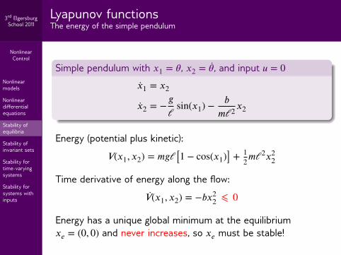
Simple pendulum with 𝑥1 = , 𝑥2 = , and input 𝑢 = 0
��1 = 𝑥2
��2 = −𝑔ℓ
sin(𝑥1) − 𝑏𝑚ℓ2 𝑥2
Energy (potential plus kinetic):
𝑉(𝑥1, 𝑥2) = 𝑚𝑔ℓ[1 − cos(𝑥1)] + 12 𝑚ℓ2𝑥2
2
Time derivative of energy along the flow:𝑉(𝑥1, 𝑥2) = −𝑏𝑥2
2 ⩽ 0
Energy has a unique global minimum at the equilibrium𝑥𝑒 = (0, 0) and never increases, so 𝑥𝑒 must be stable!

NonlinearControl
Nonlinearmodels
Nonlineardifferentialequations
Stability ofequilibria
Stability ofinvariant sets
Stability fortime-varyingsystems
Stability forsystems withinputs
3rd ElgersburgSchool 2011
Directional derivativesDerivatives along the flow of a vector field
Given:a vector field 𝑓(𝑥) on 𝑋 with flow 𝜑(𝑡, 𝑥)a C1 function 𝑉 ∶ 𝑋 → ℝ
The directional derivative or Lie derivative or timederivative of 𝑉 along 𝑓 is the function 𝐿𝑓𝑉 ∶ 𝑋 → ℝ given by
𝐿𝑓𝑉(𝑥) = 𝜕𝜕𝑡
𝑉(𝜑(𝑡, 𝑥))|||𝑡=0
The values of 𝐿𝑓𝑉 are independent of coordinates, but we cancompute them in local coordinates 𝑥 = (𝑥1, …, 𝑥𝑛) as
𝐿𝑓𝑉(𝑥) = 𝐷𝑉(𝑥) ·𝑓(𝑥) = 𝜕𝑉(𝑥)𝜕𝑥1
𝑓1(𝑥)⏟⏟⏟
��1
+ … + 𝜕𝑉(𝑥)𝜕𝑥𝑛
𝑓𝑛(𝑥)⏟⏟⏟
��𝑛
NonlinearControl
Nonlinearmodels
Nonlineardifferentialequations
Stability ofequilibria
Stability ofinvariant sets
Stability fortime-varyingsystems
Stability forsystems withinputs
3rd ElgersburgSchool 2011
Lyapunov functionsTime-invariant case
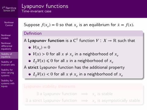
Suppose 𝑓(𝑥𝑒) = 0 so that 𝑥𝑒 is an equilibrium for �� = 𝑓(𝑥).
Definition
A Lyapunov function is a C1 function 𝑉 ∶ 𝑋 → ℝ such that𝑉(𝑥𝑒) = 0𝑉(𝑥) > 0 for all 𝑥 ≠ 𝑥𝑒 in a neighborhood of 𝑥𝑒
𝐿𝑓𝑉(𝑥) ⩽ 0 for all 𝑥 in a neighborhood of 𝑥𝑒
A strict Lyapunov function has the additional property𝐿𝑓𝑉(𝑥) < 0 for all 𝑥 ≠ 𝑥𝑒 in a neighborhood of 𝑥𝑒
Lyapunov stability theorems
∃ a Lyapunov function ⟹ 𝑥𝑒 is stable∃ a strict Lyapunov function ⟹ 𝑥𝑒 is asymptotically stable

NonlinearControl
Nonlinearmodels
Nonlineardifferentialequations
Stability ofequilibria
Stability ofinvariant sets
Stability fortime-varyingsystems
Stability forsystems withinputs
3rd ElgersburgSchool 2011
Lyapunov functionsTime-invariant case
Suppose 𝑓(𝑥𝑒) = 0 so that 𝑥𝑒 is an equilibrium for �� = 𝑓(𝑥).
Definition
A Lyapunov function is a C1 function 𝑉 ∶ 𝑋 → ℝ such that𝑉(𝑥𝑒) = 0𝑉(𝑥) > 0 for all 𝑥 ≠ 𝑥𝑒 in a neighborhood of 𝑥𝑒
𝐿𝑓𝑉(𝑥) ⩽ 0 for all 𝑥 in a neighborhood of 𝑥𝑒
A strict Lyapunov function has the additional property𝐿𝑓𝑉(𝑥) < 0 for all 𝑥 ≠ 𝑥𝑒 in a neighborhood of 𝑥𝑒
Lyapunov stability theorems
∃ a Lyapunov function ⟹ 𝑥𝑒 is stable∃ a strict Lyapunov function ⟹ 𝑥𝑒 is asymptotically stable

NonlinearControl
Nonlinearmodels
Nonlineardifferentialequations
Stability ofequilibria
Stability ofinvariant sets
Stability fortime-varyingsystems
Stability forsystems withinputs
3rd ElgersburgSchool 2011 Lyapunov function intuition
𝑉 is shaped like a bowl or a valley near 𝑥𝑒𝑥𝑒 is at the bottom of the valleythe flow cannot go uphill in forward timeif 𝑉 is strict, then the flow always goes downhill

NonlinearControl
Nonlinearmodels
Nonlineardifferentialequations
Stability ofequilibria
Stability ofinvariant sets
Stability fortime-varyingsystems
Stability forsystems withinputs
3rd ElgersburgSchool 2011
Global Lyapunov functionsTime-invariant case
𝑉 is called proper when the sublevel setsΩ𝑉(𝑐) = {𝑥 ∈ 𝑋 ∶ 𝑉(𝑥) ⩽ 𝑐}
are compact for all 𝑐 ∈ 𝑉(𝑋).
DefinitionA global Lyapunov function is a function 𝑉 ∶ 𝑋 → ℝ such that
𝑉 is C1 and proper𝑉(𝑥𝑒) = 0 and 𝑉(𝑥) > 0 for all 𝑥 ∈ 𝑋 with 𝑥 ≠ 𝑥𝑒
𝐿𝑓𝑉(𝑥) < 0 for all 𝑥 ∈ 𝑋 with 𝑥 ≠ 𝑥𝑒
Global stability theorem∃ a global Lyapunov function
⇓𝑥𝑒 is globally asymptotically stable

NonlinearControl
Nonlinearmodels
Nonlineardifferentialequations
Stability ofequilibria
Stability ofinvariant sets
Stability fortime-varyingsystems
Stability forsystems withinputs
3rd ElgersburgSchool 2011
Global Lyapunov functionsLTI systems
LTI system with equilibrium 𝑥𝑒 = 0 and Hurwitz 𝐴
�� = 𝐴𝑥
Lyapunov matrix equationIf 𝐴 is Hurwitz, then for any 𝑄 > 0 there exists 𝑃 > 0 such that
𝐴𝑇𝑃 + 𝑃𝐴 + 𝑄 = 0
Global Lyapunov function
The quadratic function 𝑉(𝑥) = 𝑥𝑇𝑃 𝑥 has time derivative𝑉(𝑥) = −𝑥𝑇𝑄𝑥, so
𝑉 is a global Lyapunov functionthus 𝑥𝑒 = 0 is globally asymptotically stable

NonlinearControl
Nonlinearmodels
Nonlineardifferentialequations
Stability ofequilibria
Stability ofinvariant sets
Stability fortime-varyingsystems
Stability forsystems withinputs
3rd ElgersburgSchool 2011 Lyapunov functions for linearized systems
suppose �� = 𝑓(𝑥) with 𝑓(0) = 0 (equilibrium at 𝑥𝑒 = 0)
suppose the Jacobian matrix 𝐴 = 𝐷𝑓(0) is Hurwitz
write the system as
�� = 𝐴𝑥 + higher-order terms
choose 𝑄 > 0 and solve 𝐴𝑇𝑃 + 𝑃𝐴 + 𝑄 = 0 for 𝑃 > 0
quadratic 𝑉(𝑥) = 𝑥𝑇𝑃 𝑥 satisfies
𝐿𝑓𝑉(𝑥) = −𝑥𝑇𝑄𝑥 + higher-order terms
𝑉 is a strict Lyapunov function, so 𝑥𝑒 is asymp. stable
use 𝑉 to estimate the region of attraction 𝑊 𝑠(𝑥𝑒) …
NonlinearControl
Nonlinearmodels
Nonlineardifferentialequations
Stability ofequilibria
Stability ofinvariant sets
Stability fortime-varyingsystems
Stability forsystems withinputs
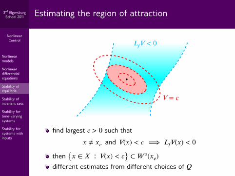
3rd ElgersburgSchool 2011 Estimating the region of attraction
𝐿𝑓𝑉 < 0
𝑉 = 𝑐
find largest 𝑐 > 0 such that
𝑥 ≠ 𝑥𝑒 and 𝑉(𝑥) < 𝑐 ⟹ 𝐿𝑓𝑉(𝑥) < 0
then {𝑥 ∈ 𝑋 ∶ 𝑉(𝑥) < 𝑐} ⊂ 𝑊 𝑠(𝑥𝑒)different estimates from different choices of 𝑄

NonlinearControl
Nonlinearmodels
Nonlineardifferentialequations
Stability ofequilibria
Stability ofinvariant sets
Stability fortime-varyingsystems
Stability forsystems withinputs
3rd ElgersburgSchool 2011 Asymptotic stability of the simple pendulum
For zero input 𝑢 = 0, the energy function
𝑉(𝑥1, 𝑥2) = 𝑚𝑔ℓ[1 − cos(𝑥1)] + 12 𝑚ℓ2𝑥2
2
satisfies𝐿𝑓𝑉(𝑥1, 𝑥2) = −𝑏𝑥2
2
and is thus a Lyapunov function for the equilibrium 𝑥𝑒 = (0, 0).
𝑉 is not a strict Lyapunov function, but 𝑥𝑒 is asymptoticallystable nonetheless when 𝑏 > 0.
To prove asymptotic stability, we canlook for a strict Lyapunov function, oruse the invariance principle …

NonlinearControl
Nonlinearmodels
Nonlineardifferentialequations
Stability ofequilibria
Stability ofinvariant sets
Stability fortime-varyingsystems
Stability forsystems withinputs
3rd ElgersburgSchool 2011 Invariant sets
Let 𝜑(𝑡, 𝑥) be the flow of a vector field 𝑓(𝑥) on 𝑋.
DefinitionA subset Γ ⊂ 𝑋 is called
invariant when 𝑥 ∈ Γ implies 𝜑(𝑡, 𝑥) ∈ Γ for all 𝑡 ∈ ℐ(𝑥)forward-invariant when 𝑥 ∈ Γ implies 𝜑(𝑡, 𝑥) ∈ Γ for allpositive 𝑡 ∈ ℐ(𝑥)
Invariant sets include:equilibria, stable sets of equilibria, periodic orbits(including limit cycles)the orbit 𝜑(ℐ(𝑥), 𝑥) through any 𝑥 ∈ 𝑋
Forward-invariant sets that need not be invariant include:the sublevel sets Ω𝑉(𝑐) of a Lyapunov function

NonlinearControl
Nonlinearmodels
Nonlineardifferentialequations
Stability ofequilibria
Stability ofinvariant sets
Stability fortime-varyingsystems
Stability forsystems withinputs
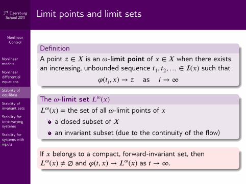
3rd ElgersburgSchool 2011 Limit points and limit sets
DefinitionA point 𝑧 ∈ 𝑋 is an 𝜔-limit point of 𝑥 ∈ 𝑋 when there existsan increasing, unbounded sequence 𝑡1, 𝑡2, … ∈ ℐ(𝑥) such that
𝜑(𝑡𝑖, 𝑥) → 𝑧 as 𝑖 → ∞
The 𝜔-limit set 𝐿𝜔(𝑥)𝐿𝜔(𝑥) = the set of all 𝜔-limit points of 𝑥
a closed subset of 𝑋an invariant subset (due to the continuity of the flow)
If 𝑥 belongs to a compact, forward-invariant set, then𝐿𝜔(𝑥) ≠ ∅ and 𝜑(𝑡, 𝑥) → 𝐿𝜔(𝑥) as 𝑡 → ∞.
NonlinearControl
Nonlinearmodels
Nonlineardifferentialequations
Stability ofequilibria
Stability ofinvariant sets
Stability fortime-varyingsystems
Stability forsystems withinputs
3rd ElgersburgSchool 2011 Limit points and limit sets
DefinitionA point 𝑧 ∈ 𝑋 is an 𝜔-limit point of 𝑥 ∈ 𝑋 when there existsan increasing, unbounded sequence 𝑡1, 𝑡2, … ∈ ℐ(𝑥) such that
𝜑(𝑡𝑖, 𝑥) → 𝑧 as 𝑖 → ∞
The 𝜔-limit set 𝐿𝜔(𝑥)𝐿𝜔(𝑥) = the set of all 𝜔-limit points of 𝑥
a closed subset of 𝑋an invariant subset (due to the continuity of the flow)
If 𝑥 belongs to a compact, forward-invariant set, then𝐿𝜔(𝑥) ≠ ∅ and 𝜑(𝑡, 𝑥) → 𝐿𝜔(𝑥) as 𝑡 → ∞.

NonlinearControl
Nonlinearmodels
Nonlineardifferentialequations
Stability ofequilibria
Stability ofinvariant sets
Stability fortime-varyingsystems
Stability forsystems withinputs
3rd ElgersburgSchool 2011 LaSalle's invariance principle
AssumeΩ ⊂ 𝑋 is compact and forward-invariantthere is a C1 function 𝑉(𝑥) on 𝑋 such that 𝐿𝑓𝑉(𝑥) ⩽ 0 on Ω
Define the set𝐸 = {𝑥 ∈ Ω ∶ 𝐿𝑓𝑉(𝑥) = 0}
Invariance principleIf 𝑥 ∈ Ω then sup ℐ(𝑥) = ∞ and 𝜑(𝑡, 𝑥) → 𝑀 as 𝑡 → ∞,where 𝑀 is largest invariant subset of 𝐸.
𝑡 ↦ 𝑉(𝜑(𝑡, 𝑥)) is bounded from below and nonincreasing,and thus approaches a limithence 𝑉 is constant on 𝐿𝜔(𝑥), which means 𝐿𝜔(𝑥) ⊂ 𝐸because 𝐿𝜔(𝑥) is invariant𝜑(𝑡, 𝑥) → 𝐿𝜔(𝑥) ⊂ 𝑀 as 𝑡 → ∞

NonlinearControl
Nonlinearmodels
Nonlineardifferentialequations
Stability ofequilibria
Stability ofinvariant sets
Stability fortime-varyingsystems
Stability forsystems withinputs
3rd ElgersburgSchool 2011
LaSalle's invariance principleSimple pendulum example
For zero input 𝑢 = 0, the energy function
𝑉(𝑥1, 𝑥2) = 𝑚𝑔ℓ[1 − cos(𝑥1)] + 12 𝑚ℓ2𝑥2
2
satisfies𝐿𝑓𝑉(𝑥1, 𝑥2) = −𝑏𝑥2
2
For each fixed 𝑥0 ∈ 𝑋:choose Ω = Ω𝑉(𝑉(𝑥0)) = {𝑥 ∈ 𝑋 ∶ 𝑉(𝑥) ⩽ 𝑉(𝑥0)}Ω is compact because 𝑉 is properand forward-invariant because 𝐿𝑓𝑉 ⩽ 0𝐸 = {𝑥 ∈ Ω ∶ 𝐿𝑓𝑉(𝑥) = 0} = {𝑉(𝑥) ⩽ 𝑉(𝑥0) and 𝑥2 = 0}𝑀 = {(0, 0)} if 𝑉(𝑥0) < 2𝑚𝑔ℓ, else 𝑀 = {(0, 0), (𝜋, 0)}
Every trajectory converges either to (0, 0) or to (𝜋, 0).If 𝑉(𝑥0) < 2𝑚𝑔ℓ then the trajectory converges to (0, 0).

NonlinearControl
Nonlinearmodels
Nonlineardifferentialequations
Stability ofequilibria
Stability ofinvariant sets
Stability fortime-varyingsystems
Stability forsystems withinputs
3rd ElgersburgSchool 2011 Outline
1 Nonlinear models
2 Nonlinear differential equations
3 Stability of equilibria
4 Stability of invariant sets
5 Stability for time-varying systems
6 Stability for systems with inputs

NonlinearControl
Nonlinearmodels
Nonlineardifferentialequations
Stability ofequilibria
Stability ofinvariant sets
Stability fortime-varyingsystems
Stability forsystems withinputs
3rd ElgersburgSchool 2011 Stability of invariant sets
replace equilibrium 𝑥𝑒 with any compact invariant setmost stability definitions and results are unchanged
Example on 𝑋 = ℝ2
��1 = 𝜌(𝑥)[1 − 𝜌(𝑥)]𝑥1 − 𝑥2
��2 = 𝜌(𝑥)[1 − 𝜌(𝑥)]𝑥2 + 𝑥1 where 𝜌(𝑥) = 𝑥21 + 𝑥2
2
the unit circle {𝜌(𝑥) = 1} is an invariant set consisting ofthe periodic orbit (𝑥1(𝑡), 𝑥2(𝑡)) = (cos(𝑡), sin(𝑡))asymptotic stability: do trajectories which start near theunit circle stay near it and converge to it?
Try 𝑉(𝑥) = [1 − 𝜌(𝑥)]2 and apply LaSalle …

NonlinearControl
Nonlinearmodels
Nonlineardifferentialequations
Stability ofequilibria
Stability ofinvariant sets
Stability fortime-varyingsystems
Stability forsystems withinputs
3rd ElgersburgSchool 2011 Asymptotic stability of a periodic orbit
𝑉(𝑥) = [1 − 𝜌(𝑥)]2
𝐿𝑓𝑉(𝑥) = −4𝜌2(𝑥)[1 − 𝜌(𝑥)]2 ⩽ 0
Ω = {𝑥 ∈ 𝑋 ∶ 1𝑐 ⩽ 𝜌(𝑥) ⩽ 𝑐}
annulus Ω is compact and forward-invariant for any 𝑐 ⩾ 1
for 𝑥0 ≠ 0 choose 𝑐 ⩾ 1 so that 𝑥0 ∈ Ω
𝐸 = {𝑥 ∈ Ω ∶ 𝐿𝑓𝑉(𝑥) = 0} = {𝑥 ∈ 𝑋 ∶ 𝜌(𝑥) = 1}thus all nonzero trajectories converge to the periodic orbit
NonlinearControl
Nonlinearmodels
Nonlineardifferentialequations
Stability ofequilibria
Stability ofinvariant sets
Stability fortime-varyingsystems
Stability forsystems withinputs
3rd ElgersburgSchool 2011 Outline
1 Nonlinear models
2 Nonlinear differential equations
3 Stability of equilibria
4 Stability of invariant sets
5 Stability for time-varying systems
6 Stability for systems with inputs
NonlinearControl
Nonlinearmodels
Nonlineardifferentialequations
Stability ofequilibria
Stability ofinvariant sets
Stability fortime-varyingsystems
Stability forsystems withinputs
3rd ElgersburgSchool 2011 Trajectory tracking
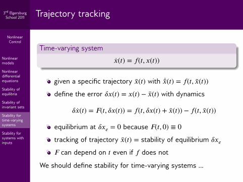
Time-varying system
��(𝑡) = 𝑓(𝑡, 𝑥(𝑡))
given a specific trajectory ��(𝑡) with ��(𝑡) = 𝑓(𝑡, ��(𝑡))
define the error 𝛿𝑥(𝑡) = 𝑥(𝑡) − ��(𝑡) with dynamics
𝛿��(𝑡) = 𝐹(𝑡, 𝛿𝑥(𝑡)) = 𝑓(𝑡, 𝛿𝑥(𝑡) + ��(𝑡)) − 𝑓(𝑡, ��(𝑡))
equilibrium at 𝛿𝑥𝑒 = 0 because 𝐹(𝑡, 0) ≡ 0
tracking of trajectory ��(𝑡) = stability of equilibrium 𝛿𝑥𝑒
𝐹 can depend on 𝑡 even if 𝑓 does not
We should define stability for time-varying systems …
NonlinearControl
Nonlinearmodels
Nonlineardifferentialequations
Stability ofequilibria
Stability ofinvariant sets
Stability fortime-varyingsystems
Stability forsystems withinputs
3rd ElgersburgSchool 2011
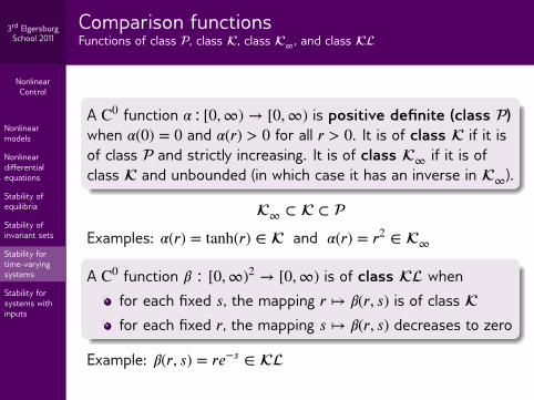
Comparison functionsFunctions of class 𭒫, class 𭒦, class 𭒦∞, and class 𭒦ℒ
A C0 function 𝛼∶[0, ∞) → [0, ∞) is positive definite (class 𭒫)when 𝛼(0) = 0 and 𝛼(𝑟) > 0 for all 𝑟 > 0. It is of class 𭒦 if it isof class 𭒫 and strictly increasing. It is of class 𭒦∞ if it is ofclass 𭒦 and unbounded (in which case it has an inverse in 𭒦∞).
𭒦∞ ⊂ 𭒦 ⊂ 𭒫
Examples: 𝛼(𝑟) = tanh(𝑟) ∈ 𭒦 and 𝛼(𝑟) = 𝑟2 ∈ 𭒦∞
A C0 function 𝛽 ∶ [0, ∞)2 → [0, ∞) is of class 𭒦ℒ whenfor each fixed 𝑠, the mapping 𝑟 ↦ 𝛽(𝑟, 𝑠) is of class 𭒦for each fixed 𝑟, the mapping 𝑠 ↦ 𝛽(𝑟, 𝑠) decreases to zero
Example: 𝛽(𝑟, 𝑠) = 𝑟𝑒−𝑠 ∈ 𭒦ℒ

NonlinearControl
Nonlinearmodels
Nonlineardifferentialequations
Stability ofequilibria
Stability ofinvariant sets
Stability fortime-varyingsystems
Stability forsystems withinputs
3rd ElgersburgSchool 2011 Uniform stability
Time-varying system with an equilibrium at zero
��(𝑡) = 𝑓(𝑡, 𝑥(𝑡)) 𝑥(𝑡0) = 𝑥0 𝑓(𝑡, 0) ≡ 0
DefinitionThe equilibrium is uniformly stable when there exists aclass-𭒦 function 𝛼 such that
|𝑥(𝑡)| ⩽ 𝛼(|𝑥0|)
for all 𝑡0, for all 𝑡 ⩾ 𝑡0, and for all 𝑥0 in a neighborhood of zero.
Uniform stability: trajectories that start nearby stay nearby,and the notion of nearby does not depend on 𝑡0.

NonlinearControl
Nonlinearmodels
Nonlineardifferentialequations
Stability ofequilibria
Stability ofinvariant sets
Stability fortime-varyingsystems
Stability forsystems withinputs
3rd ElgersburgSchool 2011 Uniform asymptotic stability
DefinitionThe equilibrium is uniformly asymptotically stable whenthere exists a class-𭒦ℒ function 𝛽 such that
|𝑥(𝑡)| ⩽ 𝛽(|𝑥0|, 𝑡 − 𝑡0)
for all 𝑡0, for all 𝑡 ⩾ 𝑡0, and for all 𝑥0 in a neighborhood of zero.
Uniformasymptoticstability
=uniform stability
+decay that depends only on the
elapsed time 𝑡 − 𝑡0
Global uniform asymptotic stability: above holds for all 𝑥0 ∈ 𝑋(must give global meaning to |·| if 𝑋 is not an open subset of ℝ𝑛)

NonlinearControl
Nonlinearmodels
Nonlineardifferentialequations
Stability ofequilibria
Stability ofinvariant sets
Stability fortime-varyingsystems
Stability forsystems withinputs
3rd ElgersburgSchool 2011
Lyapunov functionsTime-varying case
Let 𝑉 ∶ ℝ × 𝑋 → ℝ be C1 and such that for some 𝛼1, 𝛼2 ∈ 𭒦,
𝛼1(|𝑥|) ⩽ 𝑉(𝑡, 𝑥) ⩽ 𝛼2(|𝑥|) ∀𝑡 and ∀𝑥 near zero
if the time derivative of 𝑉 along trajectories satisfies
𝑉(𝑡, 𝑥) = 𝜕𝑉(𝑡, 𝑥)𝜕𝑡
+ 𝜕𝑉(𝑡, 𝑥)𝜕𝑥
𝑓(𝑡, 𝑥) ⩽ 0
∀𝑡 and ∀𝑥 near zero, then 𝑉 is a Lyapunov function
if in addition there exists 𝛼3 ∈ 𭒫 such that𝑉(𝑡, 𝑥) ⩽ −𝛼3(|𝑥|) ∀𝑡 and ∀𝑥 near zero
then 𝑉 is a strict Lyapunov function
if in addition 𝑋 = ℝ𝑛, 𝛼1 ∈ 𭒦∞, and all of these inequalitieshold for all 𝑥 ∈ 𝑋, then 𝑉 is a global Lyapunov function

NonlinearControl
Nonlinearmodels
Nonlineardifferentialequations
Stability ofequilibria
Stability ofinvariant sets
Stability fortime-varyingsystems
Stability forsystems withinputs
3rd ElgersburgSchool 2011
Lyapunov stability theoremsTime-varying case
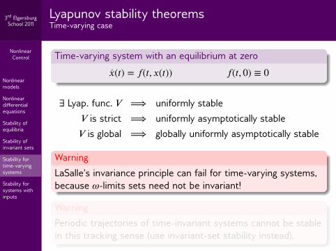
Time-varying system with an equilibrium at zero
��(𝑡) = 𝑓(𝑡, 𝑥(𝑡)) 𝑓(𝑡, 0) ≡ 0
∃ Lyap. func. 𝑉 ⟹ uniformly stable𝑉 is strict ⟹ uniformly asymptotically stable𝑉 is global ⟹ globally uniformly asymptotically stable
WarningLaSalle's invariance principle can fail for time-varying systems,because 𝜔-limits sets need not be invariant!
WarningPeriodic trajectories of time-invariant systems cannot be stablein this tracking sense (use invariant-set stability instead).
NonlinearControl
Nonlinearmodels
Nonlineardifferentialequations
Stability ofequilibria
Stability ofinvariant sets
Stability fortime-varyingsystems
Stability forsystems withinputs
3rd ElgersburgSchool 2011
Lyapunov stability theoremsTime-varying case
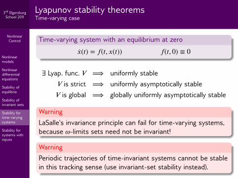
Time-varying system with an equilibrium at zero
��(𝑡) = 𝑓(𝑡, 𝑥(𝑡)) 𝑓(𝑡, 0) ≡ 0
∃ Lyap. func. 𝑉 ⟹ uniformly stable𝑉 is strict ⟹ uniformly asymptotically stable𝑉 is global ⟹ globally uniformly asymptotically stable
WarningLaSalle's invariance principle can fail for time-varying systems,because 𝜔-limits sets need not be invariant!
WarningPeriodic trajectories of time-invariant systems cannot be stablein this tracking sense (use invariant-set stability instead).

NonlinearControl
Nonlinearmodels
Nonlineardifferentialequations
Stability ofequilibria
Stability ofinvariant sets
Stability fortime-varyingsystems
Stability forsystems withinputs
3rd ElgersburgSchool 2011
Convergence using non-strict Lyapunov functionsTime-varying case
Given:system �� = 𝑓(𝑡, 𝑥) with 𝑓(𝑡, 0) ≡ 0 (equilibrium at zero)∃𝑐 > 0 such that ∀𝑡 and ∀𝑥 near zero, |𝑓(𝑡, 𝑥)| ⩽ 𝑐non-strict Lyapunov function 𝑉(𝑡, 𝑥)
Suppose there is a nonnegative C0 function 𝑊(𝑥) such that𝑉(𝑡, 𝑥) ⩽ −𝑊(𝑥) ∀𝑡 and ∀𝑥 near zero
by uniform stability, 𝑥(𝑡) stays near zero for small 𝑥0
thus ��(𝑡) is bounded ⟹ 𝑥(𝑡) & 𝑊(𝑥(𝑡)) are uniformly C0
∫ 𝑡𝑡0
𝑊(𝑥(𝜏)) 𝑑𝜏 ⩽ 𝑉(𝑡0, 𝑥0) for all 𝑡 ⩾ 𝑡0, and therefore:
If 𝑥0 is near zero, then
𝑊(𝑥(𝑡)) → 0 as 𝑡 → ∞ (Barbalat's lemma)
NonlinearControl
Nonlinearmodels
Nonlineardifferentialequations
Stability ofequilibria
Stability ofinvariant sets
Stability fortime-varyingsystems
Stability forsystems withinputs
3rd ElgersburgSchool 2011 Outline
1 Nonlinear models
2 Nonlinear differential equations
3 Stability of equilibria
4 Stability of invariant sets
5 Stability for time-varying systems
6 Stability for systems with inputs
NonlinearControl
Nonlinearmodels
Nonlineardifferentialequations
Stability ofequilibria
Stability ofinvariant sets
Stability fortime-varyingsystems
Stability forsystems withinputs
3rd ElgersburgSchool 2011
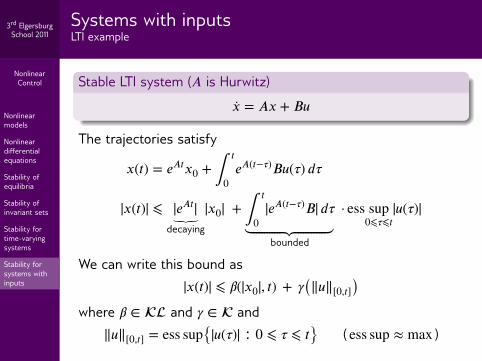
Systems with inputsLTI example
Stable LTI system (𝐴 is Hurwitz)
�� = 𝐴𝑥 + 𝐵𝑢
The trajectories satisfy
𝑥(𝑡) = 𝑒𝐴𝑡𝑥0 + ∫𝑡
0𝑒𝐴(𝑡−𝜏)𝐵𝑢(𝜏) 𝑑𝜏
|𝑥(𝑡)| ⩽ |𝑒𝐴𝑡|⏟
decaying
|𝑥0| + ∫𝑡
0|𝑒𝐴(𝑡−𝜏)𝐵| 𝑑𝜏
⏟⏟⏟⏟⏟⏟⏟⏟⏟⏟⏟⏟⏟⏟⏟⏟⏟⏟⏟⏟⏟⏟⏟bounded
· ess sup0⩽𝜏⩽𝑡
|𝑢(𝜏)|
We can write this bound as|𝑥(𝑡)| ⩽ 𝛽(|𝑥0|, 𝑡) + 𝛾(‖𝑢‖[0,𝑡])
where 𝛽 ∈ 𭒦ℒ and 𝛾 ∈ 𭒦 and‖𝑢‖[0,𝑡] = ess sup{|𝑢(𝜏)| ∶ 0 ⩽ 𝜏 ⩽ 𝑡} ( ess sup ≈ max )

NonlinearControl
Nonlinearmodels
Nonlineardifferentialequations
Stability ofequilibria
Stability ofinvariant sets
Stability fortime-varyingsystems
Stability forsystems withinputs
3rd ElgersburgSchool 2011 Input-to-state stability (ISS)
Time-varying system with inputs, 𝑋 = ℝ𝑛, 𝑢 ∈ ℝ𝑚
��(𝑡) = 𝑓(𝑡, 𝑥(𝑡), 𝑢(𝑡)) 𝑥(𝑡0) = 𝑥0
DefinitionThe system is input-to-state stable (ISS) when there exist𝛽 ∈ 𭒦ℒ and 𝛾 ∈ 𭒦 such that for any admissible 𝑢(𝑡),
|𝑥(𝑡)| ⩽ 𝛽(|𝑥0|, 𝑡 − 𝑡0) + 𝛾(‖𝑢‖[𝑡0,𝑡])
for all 𝑡0, for all 𝑡 ⩾ 𝑡0, and for all 𝑥0 ∈ 𝑋.
when 𝑢 ≡ 0, an ISS system has a globally uniformlyasymptotically stable equilibrium at zerothe class-𭒦 function 𝛾 is called the gain function

NonlinearControl
Nonlinearmodels
Nonlineardifferentialequations
Stability ofequilibria
Stability ofinvariant sets
Stability fortime-varyingsystems
Stability forsystems withinputs
3rd ElgersburgSchool 2011 Example: globally asymptotically stable but not ISS
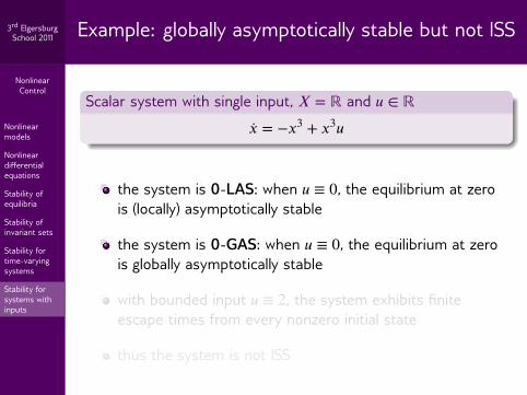
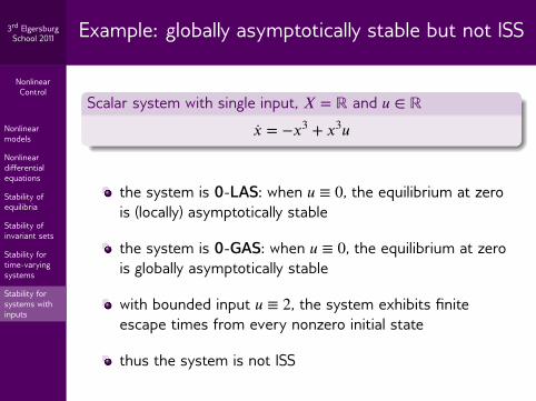
Scalar system with single input, 𝑋 = ℝ and 𝑢 ∈ ℝ
�� = −𝑥3 + 𝑥3𝑢
the system is 0-LAS: when 𝑢 ≡ 0, the equilibrium at zerois (locally) asymptotically stable
the system is 0-GAS: when 𝑢 ≡ 0, the equilibrium at zerois globally asymptotically stable
with bounded input 𝑢 ≡ 2, the system exhibits finiteescape times from every nonzero initial state
thus the system is not ISS
NonlinearControl
Nonlinearmodels
Nonlineardifferentialequations
Stability ofequilibria
Stability ofinvariant sets
Stability fortime-varyingsystems
Stability forsystems withinputs
3rd ElgersburgSchool 2011 Example: globally asymptotically stable but not ISS
Scalar system with single input, 𝑋 = ℝ and 𝑢 ∈ ℝ
�� = −𝑥3 + 𝑥3𝑢
the system is 0-LAS: when 𝑢 ≡ 0, the equilibrium at zerois (locally) asymptotically stable
the system is 0-GAS: when 𝑢 ≡ 0, the equilibrium at zerois globally asymptotically stable
with bounded input 𝑢 ≡ 2, the system exhibits finiteescape times from every nonzero initial state
thus the system is not ISS

NonlinearControl
Nonlinearmodels
Nonlineardifferentialequations
Stability ofequilibria
Stability ofinvariant sets
Stability fortime-varyingsystems
Stability forsystems withinputs
3rd ElgersburgSchool 2011 ISS Lyapunov functions
Definition
An ISS Lyapunov function is a C1 function 𝑉 ∶ ℝ × 𝑋 → ℝsuch that for some 𝛼1, 𝛼2, 𝛼3 ∈ 𭒦∞ and some 𝛼4 ∈ 𭒦,
𝛼1(|𝑥|) ⩽ 𝑉(𝑡, 𝑥) ⩽ 𝛼2(|𝑥|) and 𝑉(𝑡, 𝑥, 𝑢) ⩽ −𝛼3(|𝑥|) + 𝛼4(|𝑢|)
for all 𝑡, 𝑥, and 𝑢.
there exists an ISS Lyapunov function⇓
the system is ISS with gain function 𝛾 > 𝛼−11 ∘ 𝛼2 ∘ 𝛼−1
3 ∘ 𝛼4
Main idea: 𝑉 is decreasing when 𝑥 is outside some sublevel setof 𝑉 whose size depends on |𝑢|.

NonlinearControl
Nonlinearmodels
Nonlineardifferentialequations
Stability ofequilibria
Stability ofinvariant sets
Stability fortime-varyingsystems
Stability forsystems withinputs
3rd ElgersburgSchool 2011 Example: verifying ISS
Scalar system with single input, 𝑋 = ℝ and 𝑢 ∈ ℝ
�� = −𝑥3 + 𝑥2𝑢
Try 𝑉(𝑥) = 𝑥2 so that 𝛼1(𝑟) = 𝛼2(𝑟) = 𝑟2 and
𝑉(𝑥, 𝑢) = −2𝑥4 + 2𝑥3𝑢⩽ −2𝑥4 + 2|𝑥|3|𝑢|
|𝑥| > |𝑢| implies 𝑉(𝑥, 𝑢) < 0 (enough to conclude ISS)
can use Young's inequality to bound 𝑉 by 𝛼3 and 𝛼4 …
NonlinearControl
Nonlinearmodels
Nonlineardifferentialequations
Stability ofequilibria
Stability ofinvariant sets
Stability fortime-varyingsystems
Stability forsystems withinputs
3rd ElgersburgSchool 2011 Young's inequality
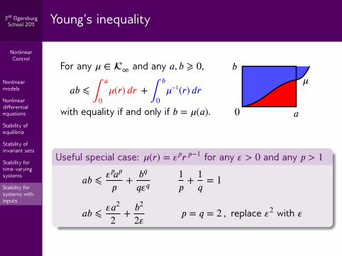
For any 𝜇 ∈ 𭒦∞ and any 𝑎, 𝑏 ⩾ 0,
𝑎𝑏 ⩽ ∫𝑎
0𝜇(𝑟) 𝑑𝑟 + ∫
𝑏
0𝜇−1(𝑟) 𝑑𝑟
with equality if and only if 𝑏 = 𝜇(𝑎). 0 𝑎
𝑏𝜇
Useful special case: 𝜇(𝑟) = 𝑝𝑟 𝑝−1 for any > 0 and any 𝑝 > 1
𝑎𝑏 ⩽𝑝𝑎𝑝
𝑝+ 𝑏𝑞
𝑞 𝑞1𝑝
+ 1𝑞
= 1
𝑎𝑏 ⩽ 𝑎2
2+ 𝑏2
2𝑝 = 𝑞 = 2 , replace 2 with
NonlinearControl
Nonlinearmodels
Nonlineardifferentialequations
Stability ofequilibria
Stability ofinvariant sets
Stability fortime-varyingsystems
Stability forsystems withinputs
3rd ElgersburgSchool 2011 Example: verifying ISS (continued)
From Young's inequality with 𝑝 = 4/3, 𝑞 = 4, = 1
|𝑥|3|𝑢| ⩽ 34 𝑥4 + 1
4 𝑢4
Thus we have the bound
𝑉(𝑥, 𝑢) ⩽ −2𝑥4 + 2|𝑥|3|𝑢|
⩽ − 12 𝑥4 + 1
2 𝑢4
so 𝛼3(𝑟) = 𝛼4(𝑟) = 12 𝑟4.
ISS with any gain function 𝛾 satisfying 𝛾(𝑟) > 𝑟 for all 𝑟 ≠ 0.

NonlinearControl
Nonlinearmodels
Nonlineardifferentialequations
Stability ofequilibria
Stability ofinvariant sets
Stability fortime-varyingsystems
Stability forsystems withinputs
3rd ElgersburgSchool 2011 Cascade interconnection of ISS systems
𝑢𝑥2��2 = 𝑓2 ��1 = 𝑓1
Cascade system with 𝑥2 as the input to the 𝑥1-subsystem
��1 = 𝑓1(𝑥1, 𝑥2) 𝑓1(0, 0) = 0��2 = 𝑓2(𝑥2, 𝑢) 𝑓2(0, 0) = 0
both subsystems are 0-LAS ⟹ cascade is 0-LAS
both subsystems are 0-GAS ⟹/ cascade is 0-GAS
both subsystems are ISS ⟹ cascade is ISS & 0-GAS

NonlinearControl
Nonlinearmodels
Nonlineardifferentialequations
Stability ofequilibria
Stability ofinvariant sets
Stability fortime-varyingsystems
Stability forsystems withinputs
3rd ElgersburgSchool 2011 Feedback interconnection of ISS systems
��2 = 𝑓2
��1 = 𝑓1𝑢1
𝑢2
𝑥2 𝑥1
Subsystem 𝑖 has inputs 𝑢𝑖 and 𝑥3−𝑖
��1 = 𝑓1(𝑥1, 𝑥2, 𝑢1) 𝑓1(0, 0, 0) = 0��2 = 𝑓2(𝑥1, 𝑥2, 𝑢2) 𝑓2(0, 0, 0) = 0
|𝑥1(𝑡)| ⩽ 𝛽1(|𝑥1(0)|, 𝑡) + 𝛾1(‖𝑥2‖[0,𝑡]) + 𝛾1(‖𝑢1‖[0,𝑡])
|𝑥2(𝑡)| ⩽ 𝛽2(|𝑥2(0)|, 𝑡) + 𝛾2(‖𝑥1‖[0,𝑡]) + 𝛾2(‖𝑢2‖[0,𝑡])

NonlinearControl
Nonlinearmodels
Nonlineardifferentialequations
Stability ofequilibria
Stability ofinvariant sets
Stability fortime-varyingsystems
Stability forsystems withinputs
3rd ElgersburgSchool 2011 ISS small-gain theorem
Small-gain condition: there exists 𝜌 ∈ 𭒦∞ such that
[(𝛾1 + 𝜌) ∘ (𝛾2 + 𝜌)](𝑟) ⩽ 𝑟 for all 𝑟 ⩾ 0
Small-gain condition for linear gains 𝛾𝑖(𝑟) = 𝛾𝑖𝑟
𝛾1𝛾2 < 1
small-gain condition ⟹ interconnection is ISS

NonlinearControl
Nonlinearmodels
Nonlineardifferentialequations
Stability ofequilibria
Stability ofinvariant sets
Stability fortime-varyingsystems
Stability forsystems withinputs
3rd ElgersburgSchool 2011 Another non-ISS system
Scalar system with single input, 𝑋 = ℝ and 𝑢 ∈ ℝ
�� = − tanh(𝑥) + 𝑢
Try 𝑉(𝑥) = ln(cosh(𝑥)) so that 𝛼1(𝑟) = 𝛼2(𝑟) = ln(cosh(𝑟)) and
𝑉(𝑥, 𝑢) = − tanh2(𝑥) + tanh(𝑥) · 𝑢⩽ − tanh2(𝑥) + |𝑢|
𝛼3(𝑟) = tanh2(𝑟), 𝛼4(𝑟) = 𝑟
cannot conclude ISS because 𝛼3 ∈ 𭒦 but 𝛼3 ∈/ 𭒦∞(in fact it is not ISS: 𝑢 ≡ 2 produces an unbounded state)
this system is integral input-to-state stable (iISS) …

NonlinearControl
Nonlinearmodels
Nonlineardifferentialequations
Stability ofequilibria
Stability ofinvariant sets
Stability fortime-varyingsystems
Stability forsystems withinputs
3rd ElgersburgSchool 2011 Integral input-to-state stability
Time-varying system with inputs, 𝑋 = ℝ𝑛, 𝑢 ∈ ℝ𝑚
��(𝑡) = 𝑓(𝑡, 𝑥(𝑡), 𝑢(𝑡)) 𝑥(𝑡0) = 𝑥0
DefinitionThe system is integral input-to-state stable (iISS) when thereexist 𝛼 ∈ 𭒦∞, 𝛽 ∈ 𭒦ℒ, and 𝛾 ∈ 𭒦 such that ∀ admissible 𝑢(𝑡),
𝛼(|𝑥(𝑡)|) ⩽ 𝛽(|𝑥0|, 𝑡 − 𝑡0) + ∫𝑡
𝑡0
𝛾(|𝑢(𝜏)|) 𝑑𝜏
for all 𝑡0, for all 𝑡 ⩾ 𝑡0, and for all 𝑥0 ∈ 𝑋.
ISS ⟹ iISS ⟹ 0-GAS

NonlinearControl
Nonlinearmodels
Nonlineardifferentialequations
Stability ofequilibria
Stability ofinvariant sets
Stability fortime-varyingsystems
Stability forsystems withinputs
3rd ElgersburgSchool 2011 iISS Lyapunov functions
Definition
An iISS Lyapunov function is a C1 function 𝑉 ∶ ℝ × 𝑋 → ℝsuch that for some 𝛼1, 𝛼2 ∈ 𭒦∞, 𝛼3 ∈ 𭒫, and 𝛼4 ∈ 𭒦,
𝛼1(|𝑥|) ⩽ 𝑉(𝑡, 𝑥) ⩽ 𝛼2(|𝑥|) and 𝑉(𝑡, 𝑥, 𝑢) ⩽ −𝛼3(|𝑥|) + 𝛼4(|𝑢|)
for all 𝑡, 𝑥, and 𝑢. Note 𝛼3 ∈ 𭒫 instead of 𝛼3 ∈ 𭒦∞.
there exists an iISS Lyapunov function⇓
the system is iISS with gain function 𝛾 = 𝛼4 for any > 0
there are cascade and small-gain theorems for iISSiISS interconnections are a recent topic of research

NonlinearControl
Controllability
Feedbackequivalence
Relative degree
Feedbacklinearization
MIMO systems
PVTOL aircraft
3rd ElgersburgSchool 2011
Part II
Feedback linearization

NonlinearControl
Controllability
Feedbackequivalence
Relative degree
Feedbacklinearization
MIMO systems
PVTOL aircraft
3rd ElgersburgSchool 2011 Outline
7 Controllability
8 Feedback equivalence
9 Relative degree
10 Feedback linearization
11 MIMO systems
12 PVTOL aircraft

NonlinearControl
Controllability
Feedbackequivalence
Relative degree
Feedbacklinearization
MIMO systems
PVTOL aircraft
3rd ElgersburgSchool 2011 A simple unicycle
𝑥
𝑦𝜃
𝑣top view States, 𝑋 = ℝ2 × 𝑆1
(𝑥1, 𝑥2, 𝑥3) = (𝑥, 𝑦, )
Controls, 𝑢 ∈ ℝ2
𝑢1 = 𝑣 = forward velocity𝑢2 = = steering velocity
Nonlinear model
��1 = 𝑢1 cos(𝑥3)��2 = 𝑢1 sin(𝑥3)��3 = 𝑢2
�� =⎡⎢⎢⎣
cos(𝑥3)sin(𝑥3)
0
⎤⎥⎥⎦
𝑢1 +⎡⎢⎢⎣
001
⎤⎥⎥⎦
𝑢2

NonlinearControl
Controllability
Feedbackequivalence
Relative degree
Feedbacklinearization
MIMO systems
PVTOL aircraft
3rd ElgersburgSchool 2011 Linear approximation of the unicycle model
Linearize the model about the equilibrium (𝑥, 𝑢) = (0, 0)
�� =⎡⎢⎢⎣
100
⎤⎥⎥⎦
𝑢1 +⎡⎢⎢⎣
001
⎤⎥⎥⎦
𝑢2 ��2 = 0
𝑥2 = 0
the state 𝑥2 is uncontrollable in the linearized system
the linearized unicycle is confined to the line 𝑥2 = 0
the nonlinear unicycle can leave this line
The linearized model does not capture the local behavior!

NonlinearControl
Controllability
Feedbackequivalence
Relative degree
Feedbacklinearization
MIMO systems
PVTOL aircraft
3rd ElgersburgSchool 2011
Vector fields and directions of motionThe simple unicycle
Unicycle model �� = 𝑔1(𝑥)𝑢1 + 𝑔2(𝑥)𝑢2 with vector fields
𝑔1(𝑥) =⎡⎢⎢⎣
cos(𝑥3)sin(𝑥3)
0
⎤⎥⎥⎦
𝑔2(𝑥) =⎡⎢⎢⎣
001
⎤⎥⎥⎦
𝑔1(𝑥) is the forward drive direction with flow 𝜑1(𝑡, 𝑥)
𝑔2(𝑥) is the ccw steer direction with flow 𝜑2(𝑡, 𝑥)
these give two directions of instantaneous motion
𝑋 = ℝ3 (locally) and thus has three independent directions
For local controllability:
Is there a 3rd independent, instantaneous direction of motion?
NonlinearControl
Controllability
Feedbackequivalence
Relative degree
Feedbacklinearization
MIMO systems
PVTOL aircraft
3rd ElgersburgSchool 2011 Wiggling the unicycle
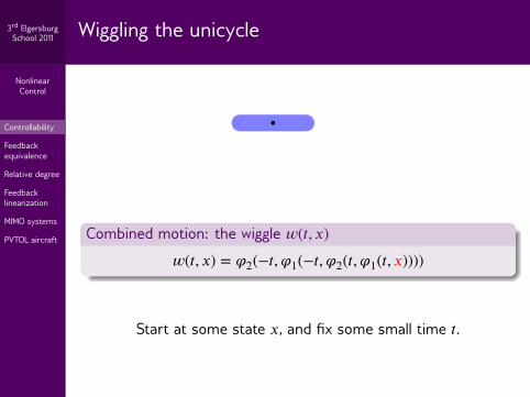
Combined motion: the wiggle 𝑤(𝑡, 𝑥)
𝑤(𝑡, 𝑥) = 𝜑2(−𝑡, 𝜑1(−𝑡, 𝜑2(𝑡, 𝜑1(𝑡, 𝑥))))
Start at some state 𝑥, and fix some small time 𝑡.

NonlinearControl
Controllability
Feedbackequivalence
Relative degree
Feedbacklinearization
MIMO systems
PVTOL aircraft
3rd ElgersburgSchool 2011 Wiggling the unicycle
Combined motion: the wiggle 𝑤(𝑡, 𝑥)
𝑤(𝑡, 𝑥) = 𝜑2(−𝑡, 𝜑1(−𝑡, 𝜑2(𝑡, 𝜑1(𝑡, 𝑥))))
Drive forward 𝑡 with (𝑢1, 𝑢2) = (1, 0).

NonlinearControl
Controllability
Feedbackequivalence
Relative degree
Feedbacklinearization
MIMO systems
PVTOL aircraft
3rd ElgersburgSchool 2011 Wiggling the unicycle
Combined motion: the wiggle 𝑤(𝑡, 𝑥)
𝑤(𝑡, 𝑥) = 𝜑2(−𝑡, 𝜑1(−𝑡, 𝜑2(𝑡, 𝜑1(𝑡, 𝑥))))
Steer counterclockwise 𝑡 with (𝑢1, 𝑢2) = (0, 1).

NonlinearControl
Controllability
Feedbackequivalence
Relative degree
Feedbacklinearization
MIMO systems
PVTOL aircraft
3rd ElgersburgSchool 2011 Wiggling the unicycle
Combined motion: the wiggle 𝑤(𝑡, 𝑥)
𝑤(𝑡, 𝑥) = 𝜑2(−𝑡, 𝜑1(−𝑡, 𝜑2(𝑡, 𝜑1(𝑡, 𝑥))))
Drive backward 𝑡 with (𝑢1, 𝑢2) = (−1, 0).

NonlinearControl
Controllability
Feedbackequivalence
Relative degree
Feedbacklinearization
MIMO systems
PVTOL aircraft
3rd ElgersburgSchool 2011 Wiggling the unicycle
Combined motion: the wiggle 𝑤(𝑡, 𝑥)
𝑤(𝑡, 𝑥) = 𝜑2(−𝑡, 𝜑1(−𝑡, 𝜑2(𝑡, 𝜑1(𝑡, 𝑥))))
Steer clockwise 𝑡 with (𝑢1, 𝑢2) = (0, −1).
NonlinearControl
Controllability
Feedbackequivalence
Relative degree
Feedbacklinearization
MIMO systems
PVTOL aircraft
3rd ElgersburgSchool 2011 Wiggling the unicycle
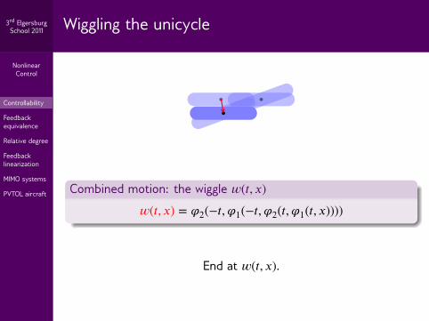
Combined motion: the wiggle 𝑤(𝑡, 𝑥)
𝑤(𝑡, 𝑥) = 𝜑2(−𝑡, 𝜑1(−𝑡, 𝜑2(𝑡, 𝜑1(𝑡, 𝑥))))
End at 𝑤(𝑡, 𝑥).

NonlinearControl
Controllability
Feedbackequivalence
Relative degree
Feedbacklinearization
MIMO systems
PVTOL aircraft
3rd ElgersburgSchool 2011 Wiggling the unicycle
Combined motion: the wiggle 𝑤(𝑡, 𝑥)
𝑤(𝑡, 𝑥) = 𝜑2(−𝑡, 𝜑1(−𝑡, 𝜑2(𝑡, 𝜑1(𝑡, 𝑥))))
What direction is the wiggle in the limit as 𝑡 → 0?Straight down, with no rotation …

NonlinearControl
Controllability
Feedbackequivalence
Relative degree
Feedbacklinearization
MIMO systems
PVTOL aircraft
3rd ElgersburgSchool 2011
A third direction of motionThe simple unicycle
Taylor expansion of the wiggle 𝑤(𝑡, 𝑥) about 𝑡 = 0
𝑤(𝑡, 𝑥) = 𝑥 +⎡⎢⎢⎣
sin(𝑥3)− cos(𝑥3)
0
⎤⎥⎥⎦⏟⏟⏟⏟⏟⏟⏟⏟⏟⏟⏟⏟⏟⏟⏟
𝑔3(𝑥)
𝑡2 + … (no linear term!)
the new direction 𝑔3(𝑥) is independent of 𝑔1(𝑥) and 𝑔2(𝑥)(it is the direction ⊥ to the forward motion of the wheel)
can move instantaneously in any direction in ℝ3 by takinglinear combinations (local controllability)
the 𝑔3 direction is slower than 𝑔1 and 𝑔2 because it appearsin the 𝑡2 term of the Taylor expansion, not the linear term

NonlinearControl
Controllability
Feedbackequivalence
Relative degree
Feedbacklinearization
MIMO systems
PVTOL aircraft
3rd ElgersburgSchool 2011 The Lie bracket of vector fields
Define wiggle for arbitrary C∞ vector fields 𝑔1(𝑥) and 𝑔2(𝑥)
𝑤(𝑡, 𝑥) = 𝜑2(−𝑡, 𝜑1(−𝑡, 𝜑2(𝑡, 𝜑1(𝑡, 𝑥)))) = 𝑥 + 𝑔3(𝑥)𝑡2 + …
The wiggle vector field 𝑔3(𝑥) turns out to be
𝑔3(𝑥) = 𝐷𝑔2(𝑥) · 𝑔1(𝑥) − 𝐷𝑔1(𝑥) · 𝑔2(𝑥) (in local coordinates)
DefinitionThe Lie bracket [𝑔1, 𝑔2] of C∞ vector fields 𝑔1(𝑥) and 𝑔2(𝑥) isthe associated wiggle vector field 𝑔3(𝑥):
[𝑔1, 𝑔2] = 𝐷𝑔2 · 𝑔1 − 𝐷𝑔1 · 𝑔2 (in local coordinates)

NonlinearControl
Controllability
Feedbackequivalence
Relative degree
Feedbacklinearization
MIMO systems
PVTOL aircraft
3rd ElgersburgSchool 2011 Some properties of the Lie bracket
Let 𝑓(𝑥), 𝑔(𝑥), and ℎ(𝑥) be C∞ vector fields on 𝑋[𝑓, 𝑔] = −[𝑔, 𝑓] (skew symmetry) ⇒ [𝑓, 𝑓] = 0
[𝑓, 𝛼𝑔 + 𝛽ℎ] = 𝛼[𝑓, 𝑔] + 𝛽[𝑓, ℎ] for 𝛼, 𝛽 ∈ ℝ (bilinearity)
[𝑓, [𝑔, ℎ]] + [ℎ, [𝑓, 𝑔]] + [𝑔, [ℎ, 𝑓]] = 0 (Jacobi identity)
for any C∞ function 𝜑(𝑥) on 𝑋,
𝐿[𝑓,𝑔]𝜑(𝑥) = 𝐿𝑓𝐿𝑔𝜑(𝑥) − 𝐿𝑔𝐿𝑓𝜑(𝑥)
Additional notationThe mapping ad𝑓(·) takes a vector field 𝑔 and produces thevector field ad𝑓(𝑔) = [𝑓, 𝑔] so that
ad0𝑓(𝑔) = 𝑔 ad1
𝑓(𝑔) = [𝑓, 𝑔] ad2𝑓(𝑔) = [𝑓, [𝑓, 𝑔]] …

NonlinearControl
Controllability
Feedbackequivalence
Relative degree
Feedbacklinearization
MIMO systems
PVTOL aircraft
3rd ElgersburgSchool 2011 Lie algebras of vector fields
𭒱(𝑋) = set of all C∞ vector fields on 𝑋
𭒱(𝑋) is a real vector space under pointwise operations
a subspace of 𭒱(𝑋) is called a Lie algebra when it isclosed under Lie brackets
given a collection {𝑓𝑖} of vector fields in 𭒱(𝑋),Lie{𝑓𝑖} = the smallest Lie algebra containing all the 𝑓𝑖
given 𝑥 ∈ 𝑋, the set
span{𝑓(𝑥) ∶ 𝑓 ∈ Lie{𝑓𝑖}}
is a subspace of ℝ𝑛 (or the tangent space of 𝑋 at 𝑥)
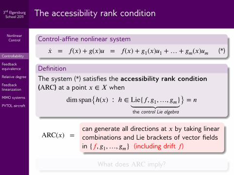
NonlinearControl
Controllability
Feedbackequivalence
Relative degree
Feedbacklinearization
MIMO systems
PVTOL aircraft
3rd ElgersburgSchool 2011 The accessibility rank condition
Control-affine nonlinear system
�� = 𝑓(𝑥) + 𝑔(𝑥)𝑢 = 𝑓(𝑥) + 𝑔1(𝑥)𝑢1 + … + 𝑔𝑚(𝑥)𝑢𝑚 (*)
DefinitionThe system (*) satisfies the accessibility rank condition(ARC) at a point 𝑥 ∈ 𝑋 when
dim span{ℎ(𝑥) ∶ ℎ ∈ Lie{𝑓, 𝑔1, …, 𝑔𝑚}⏟⏟⏟⏟⏟⏟⏟⏟⏟⏟⏟⏟⏟⏟⏟⏟⏟⏟⏟⏟⏟⏟⏟⏟⏟⏟⏟the control Lie algebra
} = 𝑛
ARC(𝑥) =can generate all directions at 𝑥 by taking linearcombinations and Lie brackets of vector fieldsin {𝑓, 𝑔1, …, 𝑔𝑚} (including drift 𝑓)
What does ARC imply?

NonlinearControl
Controllability
Feedbackequivalence
Relative degree
Feedbacklinearization
MIMO systems
PVTOL aircraft
3rd ElgersburgSchool 2011
Accessibility rank conditionLTI case
suppose 𝑓(𝑥) = 𝐴𝑥 and each 𝑔𝑖(𝑥) = 𝑔𝑖 = constant
because [𝑓, ℎ] = −𝐴ℎ for any constant ℎ, we have
dim span{ℎ(𝑥) ∶ ℎ ∈ Lie{𝑓, 𝑔1, …, 𝑔𝑚}}= rank [𝐴𝑥 𝐵 𝐴𝐵 𝐴2𝐵 … 𝐴𝑛−1𝐵]
where 𝐵 = [𝑔1 … 𝑔𝑚]
ARC(0) is the LTI controllability rank condition
if 𝑥 ≠ 0 then ARC(𝑥) may be weaker than the LTIcontrollability rank condition
What does ARC imply?

NonlinearControl
Controllability
Feedbackequivalence
Relative degree
Feedbacklinearization
MIMO systems
PVTOL aircraft
3rd ElgersburgSchool 2011
The reachable setSmall-time local accessibility and controllability
Given 𝑥 ∈ 𝑋, an open neighborhood 𝑈 of 𝑥, and a time 𝑇 > 0:
reachable set 𝑅𝑇𝑈(𝑥) =
all states that can be reachedwithin time 𝑇 starting from 𝑥and without leaving 𝑈
DefinitionThe system is small-time accessible (STA) at 𝑥 when
int 𝑅𝑇𝑈(𝑥) ≠ ∅ ∀𝑈 ∀𝑇 > 0
It is small-time locally controllable (STLC) at 𝑥 when
𝑥 ∈ int 𝑅𝑇𝑈(𝑥) ∀𝑈 ∀𝑇 > 0
Warning: inconsistent terminology in the literatureSometimes accessibility is called weak controllability.Sometimes STLC is defined with 𝑈 = 𝑋 instead of ∀𝑈.

NonlinearControl
Controllability
Feedbackequivalence
Relative degree
Feedbacklinearization
MIMO systems
PVTOL aircraft
3rd ElgersburgSchool 2011 What does ARC imply?
Sufficient conditions
ARC(𝑥) ⟹ STA at 𝑥
Necessary and sufficient conditionsARC holds on an open dense subset of 𝑋
⇕the system is STA on an open dense subset of 𝑋
Real analytic systemsARC holds on all of of 𝑋
⇕the system is STA at every 𝑥 ∈ 𝑋

NonlinearControl
Controllability
Feedbackequivalence
Relative degree
Feedbacklinearization
MIMO systems
PVTOL aircraft
3rd ElgersburgSchool 2011
What does ARC imply?Systems without drift
For systems without drift (𝑓 ≡ 0)
STA at 𝑥 ⟺ STLC at 𝑥
ARC(𝑥) ⟹ STLC at 𝑥
ARC holds on an open dense subset of 𝑋⇕
the system is STLC on an open dense subset of 𝑋
the system is completely controllable⇑ (𝑋 is connected)
ARC holds on all of of 𝑋⇓ ⇑ (system is real analytic)
the system is STLC at every 𝑥 ∈ 𝑋

NonlinearControl
Controllability
Feedbackequivalence
Relative degree
Feedbacklinearization
MIMO systems
PVTOL aircraft
3rd ElgersburgSchool 2011 Outline
7 Controllability
8 Feedback equivalence
9 Relative degree
10 Feedback linearization
11 MIMO systems
12 PVTOL aircraft

NonlinearControl
Controllability
Feedbackequivalence
Relative degree
Feedbacklinearization
MIMO systems
PVTOL aircraft
3rd ElgersburgSchool 2011
Feedback equivalenceStatic state feedback
start with a system�� = 𝑓(𝑥) + 𝑔(𝑥)𝑢
apply static state feedback
𝑢 = 𝛼(𝑥) + 𝛽(𝑥)𝑣
to get a system with a new input 𝑣
�� = 𝑓(𝑥) + 𝑔(𝑥)𝛼(𝑥) + 𝑔(𝑥)𝛽(𝑥)𝑣
change coordinates 𝑧 = Φ(𝑥) to obtain
𝑧 = 𝐹(𝑧) + 𝐺(𝑧)𝑣where
𝐹(Φ(𝑥)) = 𝐷Φ(𝑥)[𝑓(𝑥) + 𝑔(𝑥)𝛼(𝑥)]𝐺(Φ(𝑥)) = 𝐷Φ(𝑥)𝑔(𝑥)𝛽(𝑥)

NonlinearControl
Controllability
Feedbackequivalence
Relative degree
Feedbacklinearization
MIMO systems
PVTOL aircraft
3rd ElgersburgSchool 2011
Feedback equivalenceStatic state feedback
𝛼(𝑥) + 𝛽(𝑥)𝑣 �� = 𝑓(𝑥) + 𝑔(𝑥)𝑢 Φ 𝑧𝑣𝑥𝑢
𝑧 = 𝐹(𝑧) + 𝐺(𝑧)𝑣
Reversible feedback transformation on an open set 𝑈 ⊂ 𝑋C∞ functions 𝛼 ∶ 𝑈 → ℝ𝑚 and 𝛽 ∶ 𝑈 → ℝ𝑚×𝑚
𝛽(𝑥) is nonsingular on 𝑈Φ ∶ 𝑈 → 𝑈′ is a diffeomorphism
Why transform? The new system might be easier to use …

NonlinearControl
Controllability
Feedbackequivalence
Relative degree
Feedbacklinearization
MIMO systems
PVTOL aircraft
3rd ElgersburgSchool 2011
Feedback equivalenceStatic state feedback example
System with three states 𝑋 = ℝ3 and two inputs 𝑢 ∈ ℝ2
��1 = 𝑥21 + 𝑥2
��2 = 𝑥1𝑥2 + 𝑥23𝑢1 + 𝑢2
��3 = 𝑥1𝑥3 + 𝑢1
Static state feedback and global coordinate change
[𝑢1𝑢2] = [
−𝑥1𝑥3𝑥1𝑥3
3 − 2𝑥31 − 3𝑥1𝑥2]
⏟⏟⏟⏟⏟⏟⏟⏟⏟⏟⏟⏟⏟⏟⏟⏟⏟⏟⏟⏟⏟⏟⏟⏟⏟⏟⏟⏟⏟⏟⏟⏟⏟⏟⏟⏟⏟⏟⏟𝛼(𝑥)
+ [0 11 −𝑥2
3]⏟⏟⏟⏟⏟⏟⏟⏟⏟⏟⏟
𝛽(𝑥)
[𝑣1𝑣2]
⎡⎢⎢⎣
𝑧1𝑧2𝑧3
⎤⎥⎥⎦
= Φ(𝑥) =⎡⎢⎢⎣
𝑥1𝑥2
1 + 𝑥2𝑥3
⎤⎥⎥⎦
,⎡⎢⎢⎣
𝑥1𝑥2𝑥3
⎤⎥⎥⎦
= Φ−1(𝑧) =⎡⎢⎢⎣
𝑧1−𝑧2
1 + 𝑧2𝑧3
⎤⎥⎥⎦

NonlinearControl
Controllability
Feedbackequivalence
Relative degree
Feedbacklinearization
MIMO systems
PVTOL aircraft
3rd ElgersburgSchool 2011
Feedback equivalenceStatic state feedback example
The transformed system is LTI
𝑧 =⎡⎢⎢⎣
𝑧1𝑧2𝑧3
⎤⎥⎥⎦
=⎡⎢⎢⎣
𝑧2𝑣1𝑣2
⎤⎥⎥⎦
=⎡⎢⎢⎣
0 1 00 0 00 0 0
⎤⎥⎥⎦
𝑧
⏟⏟⏟⏟⏟⏟⏟⏟⏟⏟⏟⏟⏟⏟⏟⏟⏟𝐹(𝑧)
+⎡⎢⎢⎣
0 01 00 1
⎤⎥⎥⎦⏟⏟⏟⏟⏟
𝐺(𝑧)
𝑣
The original nonlinear system is feedback equivalent to acontrollable LTI system. This suggests a design strategy:
Feedback linearizationdesign a controller for 𝑣 using linear methods applied tothe LTI transformed systemimplement 𝑢 = 𝛼(𝑥) + 𝛽(𝑥)𝑣 on the original system

NonlinearControl
Controllability
Feedbackequivalence
Relative degree
Feedbacklinearization
MIMO systems
PVTOL aircraft
3rd ElgersburgSchool 2011 Some questions about feedback linearization
is a given system feedback equivalent to an LTI system?
if so, what is the feedback and the coordinate change?
if not, would it help to consider dynamic feedback?
what if the model nonlinearities are uncertain?
what if there are control constraints?
does the linearizing feedback lead to a good design?

NonlinearControl
Controllability
Feedbackequivalence
Relative degree
Feedbacklinearization
MIMO systems
PVTOL aircraft
3rd ElgersburgSchool 2011 Outline
7 Controllability
8 Feedback equivalence
9 Relative degree
10 Feedback linearization
11 MIMO systems
12 PVTOL aircraft
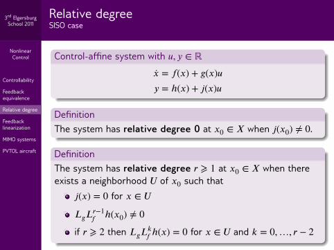
NonlinearControl
Controllability
Feedbackequivalence
Relative degree
Feedbacklinearization
MIMO systems
PVTOL aircraft
3rd ElgersburgSchool 2011
Relative degreeSISO case
Control-affine system with 𝑢, 𝑦 ∈ ℝ
�� = 𝑓(𝑥) + 𝑔(𝑥)𝑢𝑦 = ℎ(𝑥) + 𝑗(𝑥)𝑢
DefinitionThe system has relative degree 0 at 𝑥0 ∈ 𝑋 when 𝑗(𝑥0) ≠ 0.
DefinitionThe system has relative degree 𝑟 ⩾ 1 at 𝑥0 ∈ 𝑋 when thereexists a neighborhood 𝑈 of 𝑥0 such that
𝑗(𝑥) = 0 for 𝑥 ∈ 𝑈
𝐿𝑔𝐿𝑟−1𝑓 ℎ(𝑥0) ≠ 0
if 𝑟 ⩾ 2 then 𝐿𝑔𝐿𝑘𝑓 ℎ(𝑥) = 0 for 𝑥 ∈ 𝑈 and 𝑘 = 0, …, 𝑟 − 2

NonlinearControl
Controllability
Feedbackequivalence
Relative degree
Feedbacklinearization
MIMO systems
PVTOL aircraft
3rd ElgersburgSchool 2011
Relative degree and output derivativesSISO case
relative degree = number of time-derivatives of theoutput 𝑦 until the input 𝑢 appears
Example
��1 = 𝑥21 + 𝑥2
��2 = 𝑥3 + 𝑢��3 = (𝑥2 + 1)𝑥3 + 𝑥2𝑢
Relative degree 𝑟 at 𝑥0 = 0?
𝑦 = 𝑥1 ⟹ 𝑟 = 2𝑦 = 𝑥1𝑥3 + 𝑥2 ⟹ 𝑟 = 1𝑦 = 𝑥3 ⟹ 𝑟 = ??
The relative degree might not exist at every 𝑥0 ∈ 𝑋.
For SISO LTI systems, the relative degree is the pole/zeroexcess of the transfer function (#poles − #zeros).

NonlinearControl
Controllability
Feedbackequivalence
Relative degree
Feedbacklinearization
MIMO systems
PVTOL aircraft
3rd ElgersburgSchool 2011
Partial feedback linearization (I/O linearization)Normal form
If a system has relative degree 𝑟 ⩾ 1 at 𝑥0 ∈ 𝑋 then it is locally(in a neighborhood of 𝑥0) feedback equivalent to
= 𝑞( , 𝜉) ∈ ℝ𝑛−𝑟
𝜉1 = 𝜉2 𝜉 = (𝜉1, …, 𝜉𝑟) ∈ ℝ𝑟
𝜉2 = 𝜉3 𝑧 = ( , 𝜉) = Φ(𝑥)⋮
𝜉𝑟 = 𝑣 𝑣 = new input𝑦 = 𝜉1
The input/output map is the LTI system 𝑦(𝑟) = 𝑣.
Alternative form: = 𝑞( , 𝜉) + 𝑝( , 𝜉)𝑣(can be easier to calculate the coordinates)
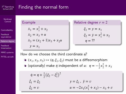
NonlinearControl
Controllability
Feedbackequivalence
Relative degree
Feedbacklinearization
MIMO systems
PVTOL aircraft
3rd ElgersburgSchool 2011 Finding the normal form
Example
��1 = 𝑥21 + 𝑥2
��2 = 𝑥3 + 𝑢��3 = (𝑥2 + 1)𝑥3 + 𝑥2𝑢𝑦 = 𝑥1
Relative degree 𝑟 = 2
𝜉1 = 𝑦 = 𝑥1
𝜉2 = 𝑦 = 𝑥21 + 𝑥2
= ??
How do we choose the third coordinate ?(𝑥1, 𝑥2, 𝑥3) ↦ ( , 𝜉1, 𝜉2) must be a diffeomorphism(optionally) make independent of 𝑢: = − 1
2 𝑥22 + 𝑥3
= + 12 (𝜉2 − 𝜉2
1)2
𝜉1 = 𝜉2 𝑦 = 𝜉1 , 𝑦 = 𝑣𝜉2 = 𝑣 𝑢 = −2𝑥1(𝑥2
1 + 𝑥2) − 𝑥3 + 𝑣

NonlinearControl
Controllability
Feedbackequivalence
Relative degree
Feedbacklinearization
MIMO systems
PVTOL aircraft
3rd ElgersburgSchool 2011 Tracking via I/O linearization
in this example, the input/output map is 𝑦 = 𝑣
thus we can design a linear controller 𝑣 for tracking areference output 𝑦ref(𝑡) having known derivatives:
𝑣 = 𝑦ref − 𝑘1(𝜉1 − 𝑦ref) − 𝑘2(𝜉2 − 𝑦ref)
this controller guarantees 𝑦(𝑡) → 𝑦ref(𝑡) as 𝑡 → ∞
this controller does not take into account the dynamics
= + 12 (𝜉2 − 𝜉2
1)2
can grow unbounded, resulting in an unbounded 𝑥 and 𝑢⟹ the zero dynamics = are unstable

NonlinearControl
Controllability
Feedbackequivalence
Relative degree
Feedbacklinearization
MIMO systems
PVTOL aircraft
3rd ElgersburgSchool 2011 Zero dynamics
Zero dynamicsThe zero dynamics are the internal state trajectories that arisewhen the output is held at zero, 𝑦(𝑡) ≡ 0. In the normal form,we set 𝜉 and 𝑣 to zero to obtain the zero dynamics
= 𝑞( , 0)
the system is minimum-phase when = 0 is anasymptotically stable equilibrium of the zero dynamics
the minimum-phase condition guarantees that the trackingcontrollers will work locally for sufficiently small 𝑦ref, 𝑦ref, …
stronger stability conditions on the zero dynamics, such asbeing ISS w.r.t. (𝜉, 𝑣), can guarantee internal boundednessfor larger initial conditions and reference signals

NonlinearControl
Controllability
Feedbackequivalence
Relative degree
Feedbacklinearization
MIMO systems
PVTOL aircraft
3rd ElgersburgSchool 2011
Zero dynamicsLTI case, frequency domain
LTI system with relative degree 𝑟 (𝑏0 ≠ 0)
𝑌(𝑠) = 𝑏(𝑠)𝑎(𝑠)
𝑈(𝑠) =𝑏0𝑠𝑛−𝑟 + 𝑏1𝑠𝑛−𝑟−1 + … + 𝑏𝑛−𝑟
𝑠𝑛 + 𝑎1𝑠𝑛−1 + … + 𝑎𝑛𝑈(𝑠)
normal form is 𝑌(𝑠) = 𝑠−𝑟𝑉(𝑠) for the new input 𝑉(𝑠), so
𝑈(𝑠) = 𝑎(𝑠)𝑠𝑟𝑏(𝑠)
𝑉(𝑠) (inverted plant)
poles at roots of 𝑏(𝑠) are rendered unobservable from 𝑦
these poles are at the plant zeros, hence zero dynamics
feedback transformation into normal form effectivelycancels plant zeros with controller poles
the simple tracking controller may lead to internalunboundedness if the plant has unstable zero dynamics

NonlinearControl
Controllability
Feedbackequivalence
Relative degree
Feedbacklinearization
MIMO systems
PVTOL aircraft
3rd ElgersburgSchool 2011 Outline
7 Controllability
8 Feedback equivalence
9 Relative degree
10 Feedback linearization
11 MIMO systems
12 PVTOL aircraft

NonlinearControl
Controllability
Feedbackequivalence
Relative degree
Feedbacklinearization
MIMO systems
PVTOL aircraft
3rd ElgersburgSchool 2011 Feedback linearization
What if the relative degree is 𝑛?the resulting normal form is the LTI system 𝑦(𝑛) = 𝑣there are no zero dynamics (vacuously minimum-phase)the system is feedback equivalent to 𝑦(𝑛) = 𝑣the system is feedback linearizable
the system is feedback equivalent to a controllable LTI system⇕
there exists an output function 𝑦 = ℎ(𝑥)for which the system has relative degree 𝑛
When does such an output function ℎ(𝑥) exist?
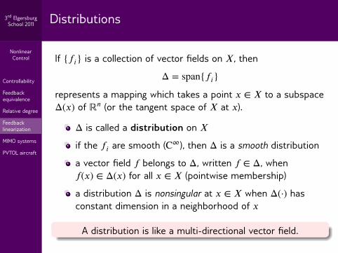
NonlinearControl
Controllability
Feedbackequivalence
Relative degree
Feedbacklinearization
MIMO systems
PVTOL aircraft
3rd ElgersburgSchool 2011 Distributions
If {𝑓𝑖} is a collection of vector fields on 𝑋, then
Δ = span{𝑓𝑖}
represents a mapping which takes a point 𝑥 ∈ 𝑋 to a subspaceΔ(𝑥) of ℝ𝑛 (or the tangent space of 𝑋 at 𝑥).
Δ is called a distribution on 𝑋
if the 𝑓𝑖 are smooth (C∞), then Δ is a smooth distribution
a vector field 𝑓 belongs to Δ, written 𝑓 ∈ Δ, when𝑓(𝑥) ∈ Δ(𝑥) for all 𝑥 ∈ 𝑋 (pointwise membership)
a distribution Δ is nonsingular at 𝑥 ∈ 𝑋 when Δ(·) hasconstant dimension in a neighborhood of 𝑥
A distribution is like a multi-directional vector field.

NonlinearControl
Controllability
Feedbackequivalence
Relative degree
Feedbacklinearization
MIMO systems
PVTOL aircraft
3rd ElgersburgSchool 2011
Frobenius theoremA multi-directional straightening-out theorem
DefinitionA distribution Δ is involutive when [Δ, Δ] ⊂ Δ, that is, when𝑓, 𝑔 ∈ Δ implies [𝑓, 𝑔] ∈ Δ.
If Δ = span{𝑓𝑖} is nonsingular, then it is involutive if and only if[𝑓𝑖, 𝑓𝑗] ∈ Δ for all 𝑖 and 𝑗 (a verifiable condition).
Frobenius theoremSuppose a distribution Δ is nonsingular at some 𝑥 ∈ 𝑋. ThenΔ is involutive in a neighborhood of 𝑥 if and only if it iscompletely integrable, that is, there exist local coordinatesaround 𝑥 in which Δ is the span of constant vector fields.

NonlinearControl
Controllability
Feedbackequivalence
Relative degree
Feedbacklinearization
MIMO systems
PVTOL aircraft
3rd ElgersburgSchool 2011 Frobenius theorem in action
Control-affine system with 𝑋 = ℝ3 and 𝑢 ∈ ℝ2
�� =⎡⎢⎢⎣
𝑥2𝑥3
𝑥22 + 𝑥1𝑥3 + 𝑥3 − 𝑥1𝑥2
⎤⎥⎥⎦⏟⏟⏟⏟⏟⏟⏟⏟⏟⏟⏟⏟⏟⏟⏟⏟⏟⏟⏟⏟⏟⏟⏟⏟⏟⏟⏟⏟⏟⏟⏟⏟⏟⏟⏟⏟⏟⏟⏟⏟⏟⏟⏟
𝑓(𝑥)
+⎡⎢⎢⎣
10𝑥2
⎤⎥⎥⎦⏟⏟⏟
𝑔1(𝑥)
𝑢1 +⎡⎢⎢⎣
01𝑥1
⎤⎥⎥⎦⏟⏟⏟
𝑔2(𝑥)
𝑢2
define Δ = span{𝑔1, 𝑔2} (nonsingular with dim Δ = 2)[𝑔1, 𝑔2] = 0 ∈ Δ, so Δ is involutive[𝑓, 𝑔1] = −𝑥2𝑔2 ∈ Δ and [𝑓, 𝑔2] = −𝑔1 − 𝑥1𝑔2 ∈ Δ⟹ [𝑓, Δ] ⊂ Δ (and we say that Δ is invariant under 𝑓 )Frobenius: there exist local coordinates 𝑧 = Φ(𝑥) in which
Δ = span{⎡⎢⎢⎣
100
⎤⎥⎥⎦
,⎡⎢⎢⎣
010
⎤⎥⎥⎦}

NonlinearControl
Controllability
Feedbackequivalence
Relative degree
Feedbacklinearization
MIMO systems
PVTOL aircraft
3rd ElgersburgSchool 2011
Frobenius theorem in actionExample continued
Because [𝑓, Δ] ⊂ Δ, we have (in the new coordinates)
[𝑓,⎡⎢⎢⎣
100
⎤⎥⎥⎦] = −
𝜕𝑓𝜕𝑧1
∈ Δ ⟹𝜕𝑓3𝜕𝑧1
≡ 0
[𝑓,⎡⎢⎢⎣
010
⎤⎥⎥⎦] = −
𝜕𝑓𝜕𝑧2
∈ Δ ⟹𝜕𝑓3𝜕𝑧2
≡ 0
Thus the third coordinate 𝑧3 has dynamics of the form
𝑧3 = 𝑓3(𝑧3)
This is an uncontrollable subsystem.
Frobenius theorem does not tell ushow to calculate these special coordinates.
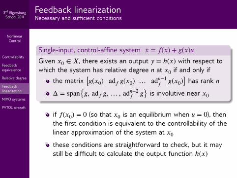
NonlinearControl
Controllability
Feedbackequivalence
Relative degree
Feedbacklinearization
MIMO systems
PVTOL aircraft
3rd ElgersburgSchool 2011
Feedback linearizationNecessary and sufficient conditions
Single-input, control-affine system �� = 𝑓(𝑥) + 𝑔(𝑥)𝑢Given 𝑥0 ∈ 𝑋, there exists an output 𝑦 = ℎ(𝑥) with respect towhich the system has relative degree 𝑛 at 𝑥0 if and only if
the matrix [𝑔(𝑥0) ad𝑓 𝑔(𝑥0) … ad𝑛−1𝑓 𝑔(𝑥0)] has rank 𝑛
Δ = span{𝑔, ad𝑓 𝑔, … , ad𝑛−2𝑓 𝑔} is involutive near 𝑥0
if 𝑓(𝑥0) = 0 (so that 𝑥0 is an equilibrium when 𝑢 = 0), thenthe first condition is equivalent to the controllability of thelinear approximation of the system at 𝑥0
these conditions are straightforward to check, but it maystill be difficult to calculate the output function ℎ(𝑥)

NonlinearControl
Controllability
Feedbackequivalence
Relative degree
Feedbacklinearization
MIMO systems
PVTOL aircraft
3rd ElgersburgSchool 2011 Outline
7 Controllability
8 Feedback equivalence
9 Relative degree
10 Feedback linearization
11 MIMO systems
12 PVTOL aircraft
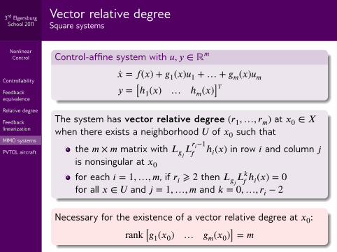
NonlinearControl
Controllability
Feedbackequivalence
Relative degree
Feedbacklinearization
MIMO systems
PVTOL aircraft
3rd ElgersburgSchool 2011
Vector relative degreeSquare systems
Control-affine system with 𝑢, 𝑦 ∈ ℝ𝑚
�� = 𝑓(𝑥) + 𝑔1(𝑥)𝑢1 + … + 𝑔𝑚(𝑥)𝑢𝑚
𝑦 = [ℎ1(𝑥) … ℎ𝑚(𝑥)]𝑇
The system has vector relative degree (𝑟1, …, 𝑟𝑚) at 𝑥0 ∈ 𝑋when there exists a neighborhood 𝑈 of 𝑥0 such that
the 𝑚 × 𝑚 matrix with 𝐿𝑔𝑗𝐿𝑟𝑖−1
𝑓 ℎ𝑖(𝑥) in row 𝑖 and column 𝑗is nonsingular at 𝑥0
for each 𝑖 = 1, …, 𝑚, if 𝑟𝑖 ⩾ 2 then 𝐿𝑔𝑗𝐿𝑘
𝑓 ℎ𝑖(𝑥) = 0for all 𝑥 ∈ 𝑈 and 𝑗 = 1, …, 𝑚 and 𝑘 = 0, …, 𝑟𝑖 − 2
Necessary for the existence of a vector relative degree at 𝑥0:
rank [𝑔1(𝑥0) … 𝑔𝑚(𝑥0)] = 𝑚

NonlinearControl
Controllability
Feedbackequivalence
Relative degree
Feedbacklinearization
MIMO systems
PVTOL aircraft
3rd ElgersburgSchool 2011
Finding the vector relative degreeDifferentiating the outputs
��1 = 𝑥21 + 𝑥3 𝑦1 = 𝑥1
��2 = 𝑥1𝑥3 + 𝑢1 𝑦2 = 𝑥2
��3 = 𝑥2 + 𝑥3𝑢1 + 𝑢2
[𝑦1𝑦2] = [
2𝑥31 + 2𝑥1𝑥3 + 𝑥2
𝑥1𝑥3 ] + [𝑥3 11 0]
⏟⏟⏟⏟⏟⏟⏟⏟⏟nonsingular
[𝑢1𝑢2] = [
𝑣1𝑣2]
the system has vector relative degree (𝑟1, 𝑟2) = (2, 1)after feedback transformation, the input/output mapbecomes 𝑦1 = 𝑣1, 𝑦2 = 𝑣2
in general, vector relative degree means feedbackequivalent to 𝑦(𝑟𝑖) = 𝑣𝑖 for 𝑖 = 1, …, 𝑚,plus zero dynamics if 𝑟1 + … + 𝑟𝑚 < 𝑛
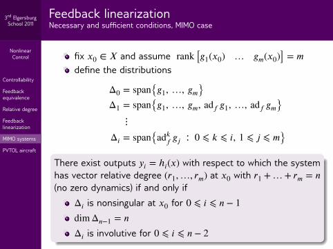
NonlinearControl
Controllability
Feedbackequivalence
Relative degree
Feedbacklinearization
MIMO systems
PVTOL aircraft
3rd ElgersburgSchool 2011
Feedback linearizationNecessary and sufficient conditions, MIMO case
fix 𝑥0 ∈ 𝑋 and assume rank [𝑔1(𝑥0) … 𝑔𝑚(𝑥0)] = 𝑚define the distributions
Δ0 = span{𝑔1, …, 𝑔𝑚}Δ1 = span{𝑔1, …, 𝑔𝑚, ad𝑓 𝑔1, …, ad𝑓 𝑔𝑚}
⋮Δ𝑖 = span{ad𝑘
𝑓 𝑔𝑗 ∶ 0 ⩽ 𝑘 ⩽ 𝑖, 1 ⩽ 𝑗 ⩽ 𝑚}
There exist outputs 𝑦𝑖 = ℎ𝑖(𝑥) with respect to which the systemhas vector relative degree (𝑟1, …, 𝑟𝑚) at 𝑥0 with 𝑟1 + … + 𝑟𝑚 = 𝑛(no zero dynamics) if and only if
Δ𝑖 is nonsingular at 𝑥0 for 0 ⩽ 𝑖 ⩽ 𝑛 − 1dim Δ𝑛−1 = 𝑛Δ𝑖 is involutive for 0 ⩽ 𝑖 ⩽ 𝑛 − 2

NonlinearControl
Controllability
Feedbackequivalence
Relative degree
Feedbacklinearization
MIMO systems
PVTOL aircraft
3rd ElgersburgSchool 2011 Checking the feedback linearization conditions
Control-affine system with 𝑋 = ℝ4 and 𝑢 ∈ ℝ2
�� =⎡⎢⎢⎢⎣
𝑥20𝑥40
⎤⎥⎥⎥⎦⏟⏟⏟
𝑓(𝑥)
+⎡⎢⎢⎢⎣
01𝑥10
⎤⎥⎥⎥⎦⏟⏟⏟
𝑔1(𝑥)
𝑢1 +⎡⎢⎢⎢⎣
0001
⎤⎥⎥⎥⎦⏟⏟⏟
𝑔2(𝑥)
𝑢2
dim Δ0 = 2[𝑔1, 𝑔2] = 0 so Δ0 is involutivedim Δ1 = 4 so Δ𝑖 is nonsingular with dim Δ𝑖 = 4(and thus Δ𝑖 is involutive) for 𝑖 ⩾ 1
The linearizing outputs 𝑦1 = ℎ1(𝑥) and 𝑦2 = ℎ2(𝑥) exist …

NonlinearControl
Controllability
Feedbackequivalence
Relative degree
Feedbacklinearization
MIMO systems
PVTOL aircraft
3rd ElgersburgSchool 2011 Finding the linearizing outputs
try 𝑦1 = 𝑥1 and 𝑦2 = 𝑥3 − 𝑥1𝑥2 :
[𝑦1𝑦2] = [
1 0−2𝑥2 1]
⏟⏟⏟⏟⏟⏟⏟⏟⏟⏟⏟⏟⏟⏟⏟nonsingular
[𝑢1𝑢2]
vector relative degree (2, 2) with no zero dynamics
what if we instead want to track 𝑦1 = 𝑥1 and 𝑦2 = 𝑥3 ?
[𝑦1𝑦2] = [
0𝑥4] + [
1 0𝑥1 0]
⏟⏟⏟⏟⏟⏟⏟⏟⏟singular
[𝑢1𝑢2]
no vector relative degree; try dynamic extension …
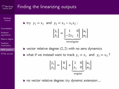

NonlinearControl
Controllability
Feedbackequivalence
Relative degree
Feedbacklinearization
MIMO systems
PVTOL aircraft
3rd ElgersburgSchool 2011
Dynamic extensionAdding integrators to achieve relative degree
introduce a controller state 𝑥5 with dynamics ��5 = 𝑢′1,
where 𝑢′1 is a new input
set 𝑢1 = 𝑥5 to achieve
[𝑦1𝑦2] = [
𝑥5𝑥4 + 𝑥1𝑥5]
take another derivative to get
[𝑦1𝑦2] = [
0𝑥2𝑥5] + [
1 0𝑥1 1]
⏟⏟⏟⏟⏟⏟⏟⏟⏟nonsingular
[𝑢′
1𝑢2]
vector relative degree (3, 2) with no zero dynamics
Dynamic feedback can be useful for achievingvector relative degree in MIMO systems.
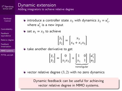

NonlinearControl
Controllability
Feedbackequivalence
Relative degree
Feedbacklinearization
MIMO systems
PVTOL aircraft
3rd ElgersburgSchool 2011 Outline
7 Controllability
8 Feedback equivalence
9 Relative degree
10 Feedback linearization
11 MIMO systems
12 PVTOL aircraft

NonlinearControl
Controllability
Feedbackequivalence
Relative degree
Feedbacklinearization
MIMO systems
PVTOL aircraft
3rd ElgersburgSchool 2011
PVTOL aircraftPlanar vertical take-off and landing aircraft
𝑥
𝑧
𝜃
𝑇
(𝑥, 𝑧) = center of mass
States, 𝑋 = ℝ4 × 𝑆1 × ℝ
(𝑥1, 𝑥2, 𝑥3, 𝑥4, 𝑥5, 𝑥6)= (𝑥, ��, 𝑧, 𝑧, , )
Controls, 𝑢 ∈ ℝ2
𝑢1 = 𝑇 = vertical thrust𝑢2 = = rotational torque
Normalized dynamics, = input coupling parameter
�� = −𝑢1 sin( ) + 𝑢2 cos( )𝑧 = 𝑢1 cos( ) + 𝑢2 sin( ) − 1 = 𝑢2

NonlinearControl
Controllability
Feedbackequivalence
Relative degree
Feedbacklinearization
MIMO systems
PVTOL aircraft
3rd ElgersburgSchool 2011
PVTOL zero dynamicsTracking the center of mass
With the output as the center of mass, (𝑦1, 𝑦2) = (𝑥, 𝑧),
[𝑦1𝑦2] = [
0−1] + [
− sin( ) cos( )cos( ) sin( )]
⏟⏟⏟⏟⏟⏟⏟⏟⏟⏟⏟⏟⏟⏟⏟⏟⏟⏟⏟⏟⏟⏟⏟⏟⏟⏟⏟⏟⏟⏟⏟⏟⏟nonsingular
[𝑢1𝑢2] = [
𝑣1𝑣2]
vector relative degree (2, 2)setting 𝑣1 = 𝑣2 = 0 yields 𝑢2 = 1
𝜀 sin( ),so the zero dynamics are
= 1𝜀 sin( )
these are the simple inverted pendulum dynamics( = 0 represents the unstable position)nonminimum-phase system;aircraft will flip over under the simple tracking control
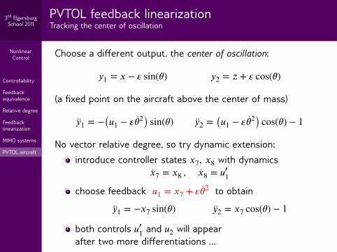
NonlinearControl
Controllability
Feedbackequivalence
Relative degree
Feedbacklinearization
MIMO systems
PVTOL aircraft
3rd ElgersburgSchool 2011
PVTOL feedback linearizationTracking the center of oscillation
Choose a different output, the center of oscillation:
𝑦1 = 𝑥 − sin( ) 𝑦2 = 𝑧 + cos( )
(a fixed point on the aircraft above the center of mass)
𝑦1 = −(𝑢1 − 2) sin( ) 𝑦2 = (𝑢1 − 2) cos( ) − 1
No vector relative degree, so try dynamic extension:introduce controller states 𝑥7, 𝑥8 with dynamics
��7 = 𝑥8 , ��8 = 𝑢′1
choose feedback 𝑢1 = 𝑥7 + 2 to obtain
𝑦1 = −𝑥7 sin( ) 𝑦2 = 𝑥7 cos( ) − 1
both controls 𝑢′1 and 𝑢2 will appear
after two more differentiations …
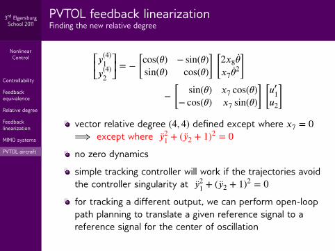
NonlinearControl
Controllability
Feedbackequivalence
Relative degree
Feedbacklinearization
MIMO systems
PVTOL aircraft
3rd ElgersburgSchool 2011
PVTOL feedback linearizationFinding the new relative degree
⎡⎢⎣𝑦(4)
1𝑦(4)
2
⎤⎥⎦
= − [cos( ) − sin( )sin( ) cos( )] [
2𝑥8 𝑥7
2]
− [sin( ) 𝑥7 cos( )
− cos( ) 𝑥7 sin( )] [𝑢′
1𝑢2]
vector relative degree (4, 4) defined except where 𝑥7 = 0⟹ except where 𝑦2
1 + ( 𝑦2 + 1)2 = 0
no zero dynamics
simple tracking controller will work if the trajectories avoidthe controller singularity at 𝑦2
1 + ( 𝑦2 + 1)2 = 0
for tracking a different output, we can perform open-looppath planning to translate a given reference signal to areference signal for the center of oscillation

NonlinearControl
Feedbackstabilization
Optimalstabilization
ControlLyapunovfunctions
Backstepping
Dissipativity
Forwarding
3rd ElgersburgSchool 2011
Part III
Stabilization

NonlinearControl
Feedbackstabilization
Optimalstabilization
ControlLyapunovfunctions
Backstepping
Dissipativity
Forwarding
3rd ElgersburgSchool 2011 Outline
13 Feedback stabilization
14 Optimal stabilization
15 Control Lyapunov functions
16 Backstepping
17 Dissipativity
18 Forwarding

NonlinearControl
Feedbackstabilization
Optimalstabilization
ControlLyapunovfunctions
Backstepping
Dissipativity
Forwarding
3rd ElgersburgSchool 2011
Stabilization via continuous state feedbackStatic feedback
Time-invariant system, 𝑥 ∈ 𝑋, 𝑢 ∈ ℝ𝑚, equilibrium at 𝑥𝑒 = 0
�� = 𝑓(𝑥, 𝑢) 𝑓(0, 0) = 0 (*)
Static state feedback
The system (*) is stabilizable via C0 static state feedback whenthere exists a C0 function 𝑘 ∶ 𝑋 → ℝ𝑚 with 𝑘(0) = 0 such that𝑥𝑒 = 0 is an asymptotically stable equilibrium of the system
�� = 𝑓(𝑥, 𝑘(𝑥))
global stabilizability when 𝑥𝑒 = 0 is GAS
time-varying feedback when 𝑢 = 𝑘(𝑡, 𝑥)

NonlinearControl
Feedbackstabilization
Optimalstabilization
ControlLyapunovfunctions
Backstepping
Dissipativity
Forwarding
3rd ElgersburgSchool 2011
Stabilization via continuous state feedbackDynamic feedback
Dynamic state feedback
The system (*) is stabilizable via C0 dynamic state feedbackwhen for some 𝑞 ⩾ 1, the augmented system
�� = 𝑓(𝑥, 𝑢) = 𝑣
with state (𝑥, ) ∈ 𝑋 × ℝ𝑞 and control (𝑢, 𝑣) ∈ ℝ𝑚 × ℝ𝑞 isstabilizable via C0 static state feedback.
the states are the internal controller states
stabilizability via dynamic state feedback does not implystabilizability via static state feedback

NonlinearControl
Feedbackstabilization
Optimalstabilization
ControlLyapunovfunctions
Backstepping
Dissipativity
Forwarding
3rd ElgersburgSchool 2011
Brockett's conditionA necessary condition for continuous stabilizability
Consider the system (*) with continuous 𝑓(·, ·)
If the system is stabilizable via C0 static or dynamic feedback,then 𝑓(·, ·) maps every neighborhood of (0, 0) ∈ 𝑋 × ℝ𝑚 to aneighborhood of 0 ∈ 𝑋.
Simple unicycle
��1 = 𝑢1 cos(𝑥3)��2 = 𝑢1 sin(𝑥3)��3 = 𝑢2
For small > 0, solve= 𝑢1 cos(𝑥3)= 𝑢1 sin(𝑥3)
0 = 𝑢2
no solution for |𝑥3| < 𝜋4
not stabilizable via C0 static or dynamic feedback
need either discontinuous or time-varying feedback

NonlinearControl
Feedbackstabilization
Optimalstabilization
ControlLyapunovfunctions
Backstepping
Dissipativity
Forwarding
3rd ElgersburgSchool 2011 Outline
13 Feedback stabilization
14 Optimal stabilization
15 Control Lyapunov functions
16 Backstepping
17 Dissipativity
18 Forwarding

NonlinearControl
Feedbackstabilization
Optimalstabilization
ControlLyapunovfunctions
Backstepping
Dissipativity
Forwarding
3rd ElgersburgSchool 2011
Optimal stabilizationCost function
Cost function with continuous 𝐿(·, ·) ⩾ 0, 𝐿(0, 0) = 0
𝐽(𝑥0, 𝑢(·)) = ∫∞
0𝐿(𝑥(𝜏), 𝑢(𝜏)) 𝑑𝜏
the integral is along trajectories of (*) under control 𝑢(·)starting at 𝑥0 (existence & uniqueness ∀𝑡 ⩾ 0 is assumed)
𝐽 may be infinite for some 𝑥0 and 𝑢(·)
𝐽 = 0 when 𝑥0 = 0 and 𝑢(·) ≡ 0 (sitting at the equilibrium)
Example: a quadratic cost function for 𝑋 = ℝ3 and 𝑢 ∈ ℝ2
𝐿(𝑥, 𝑢) = 𝑥21 + 2𝑥2
2 + 5𝑥23 + 𝑢2
1 + 10𝑢22
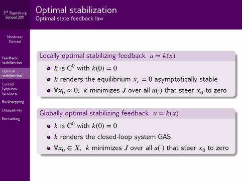
NonlinearControl
Feedbackstabilization
Optimalstabilization
ControlLyapunovfunctions
Backstepping
Dissipativity
Forwarding
3rd ElgersburgSchool 2011
Optimal stabilizationOptimal state feedback law
Locally optimal stabilizing feedback 𝑢 = 𝑘(𝑥)
𝑘 is C0 with 𝑘(0) = 0𝑘 renders the equilibrium 𝑥𝑒 = 0 asymptotically stable∀𝑥0 ≈ 0, 𝑘 minimizes 𝐽 over all 𝑢(·) that steer 𝑥0 to zero
Globally optimal stabilizing feedback 𝑢 = 𝑘(𝑥)
𝑘 is C0 with 𝑘(0) = 0𝑘 renders the closed-loop system GAS∀𝑥0 ∈ 𝑋, 𝑘 minimizes 𝐽 over all 𝑢(·) that steer 𝑥0 to zero

NonlinearControl
Feedbackstabilization
Optimalstabilization
ControlLyapunovfunctions
Backstepping
Dissipativity
Forwarding
3rd ElgersburgSchool 2011
Hamilton-Jacobi-Bellman equationA sufficient condition for optimal stabilization
suppose ∃ a C1 nonnegative function 𝑉(𝑥) with 𝑉(0) = 0which solves the Hamilton-Jacobi-Bellman equation
min𝑢∈ℝ𝑚[𝐿(𝑥, 𝑢) + 𝐷𝑉(𝑥) ·𝑓(𝑥, 𝑢)] ≡ 0
suppose there is a C0 minimizer
𝑘(𝑥) = arg min𝑢∈ℝ𝑚[𝐿(𝑥, 𝑢) + 𝐷𝑉(𝑥) ·𝑓(𝑥, 𝑢)] , 𝑘(0) = 0
which renders the system �� = 𝑓(𝑥, 𝑘(𝑥)) GAS
then 𝑢 = 𝑘(𝑥) is a globally optimal stabilizing feedback
𝑉 is called the value function

NonlinearControl
Feedbackstabilization
Optimalstabilization
ControlLyapunovfunctions
Backstepping
Dissipativity
Forwarding
3rd ElgersburgSchool 2011 Proof of optimality
if 𝑢(·) drives 𝑥0 to zero, then 𝑉(𝑥(𝑡)) → 0 as 𝑡 → ∞ and
𝐽 = 𝑉(𝑥0) + ∫∞
0[𝐿(𝑥(𝜏), 𝑢(𝜏)) + 𝐷𝑉(𝑥(𝜏)) ·𝑓(𝑥(𝜏), 𝑢(𝜏))
⏟⏟⏟⏟⏟⏟⏟⏟⏟⏟⏟⏟⏟⏟⏟⏟⏟⏟⏟⏟⏟⏟⏟⏟⏟⏟⏟⏟⏟⏟⏟⏟⏟⏟⏟⏟⏟⏟⏟𝑉(𝜏)
] 𝑑𝜏
HJB equation: integrand is ⩾ 0, and is ≡ 0 when 𝑢 = 𝑘(𝑥)
because 𝑢 = 𝑘(𝑥) is asymptotically stabilizing(by assumption), it minimizes 𝐽
the minimum value of 𝐽 is the value function 𝑉(𝑥0)
usually 𝑉 is also a Lyapunov function that verifies theasymptotic stability of the closed-loop system under thefeedback 𝑢 = 𝑘(𝑥) (note that 𝑉 = −𝐿 ⩽ 0)
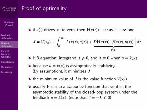

NonlinearControl
Feedbackstabilization
Optimalstabilization
ControlLyapunovfunctions
Backstepping
Dissipativity
Forwarding
3rd ElgersburgSchool 2011
Hamilton-Jacobi-Bellman equationControl-affine system with control-quadratic cost
Special case 𝑢 ∈ ℝ𝑚, 𝑔(𝑥) = [𝑔1(𝑥) … 𝑔𝑚(𝑥)]
�� = 𝑓(𝑥) + 𝑔(𝑥)𝑢 𝐿(𝑥, 𝑢) = 𝑞(𝑥) + 𝑢𝑇𝑅(𝑥)𝑢
𝑞(𝑥) ⩾ 0 and 𝑅(𝑥) = 𝑅𝑇(𝑥) > 0 for all 𝑥
with 𝐿𝑔𝑉 = [𝐿𝑔1𝑉 … 𝐿𝑔𝑚
𝑉 ], the HJB equation becomes
𝑞(𝑥) + 𝐿𝑓𝑉(𝑥) − 14 𝐿𝑔𝑉(𝑥) · 𝑅−1(𝑥) · [𝐿𝑔𝑉(𝑥)]
𝑇 = 0
the minimizing feedback law is
𝑘(𝑥) = − 12 𝑅−1(𝑥) · [𝐿𝑔𝑉(𝑥)]
𝑇
this controller has an infinite gain margin (in theory):for any 𝜌 ∈ ( 1
2 , ∞) the controller 𝑢 = 𝜌𝑘(𝑥) still stabilizesthe system

NonlinearControl
Feedbackstabilization
Optimalstabilization
ControlLyapunovfunctions
Backstepping
Dissipativity
Forwarding
3rd ElgersburgSchool 2011 Problems with the optimal stabilization approach
the HJB equation is a first-order nonlinear PDE, and can bevery difficult to solve
classical C1 solutions 𝑉(𝑥) may not even exist
even if the optimal feedback control cannot be found, acost function may still be useful in evaluating controllerperformance
if there is flexibility in the choice of 𝐿(𝑥, 𝑢), it may beeasier to claim the optimality of a feedback law(so-called inverse optimal design)
Nevertheless, there is an important special case in which wecan readily solve the HJB equation …

NonlinearControl
Feedbackstabilization
Optimalstabilization
ControlLyapunovfunctions
Backstepping
Dissipativity
Forwarding
3rd ElgersburgSchool 2011
Linear-Quadratic Regulator (LQR)LTI system, quadratic cost
Special case, 𝑄 = 𝑄𝑇 ⩾ 0, 𝑅 = 𝑅𝑇 > 0
�� = 𝐴𝑥 + 𝐵𝑢 𝐿(𝑥, 𝑢) = 𝑥𝑇𝑄𝑥 + 𝑢𝑇𝑅𝑢
if (𝐴, 𝐵) is stabilizable and (𝐴, 𝑄) is detectable, then thereis a unique positive semidefinite solution 𝑃 to thealgebraic Riccati equation
𝐴𝑇𝑃 + 𝑃𝐴 − 𝑃𝐵𝑅−1𝐵𝑇𝑃 + 𝑄 = 0
the quadratic function 𝑉(𝑥) = 𝑥𝑇𝑃 𝑥 solves HJB, and𝑘(𝑥) = −𝑅−1𝐵𝑇𝑃 𝑥
is the corresponding globally optimal stabilizing feedback
For nonlinear systems with a stabilizable linearizationWe can solve the LQR problem to discover how a nonlinearfeedback law should look near 𝑥 = 0 for local optimality.

NonlinearControl
Feedbackstabilization
Optimalstabilization
ControlLyapunovfunctions
Backstepping
Dissipativity
Forwarding
3rd ElgersburgSchool 2011 Outline
13 Feedback stabilization
14 Optimal stabilization
15 Control Lyapunov functions
16 Backstepping
17 Dissipativity
18 Forwarding

NonlinearControl
Feedbackstabilization
Optimalstabilization
ControlLyapunovfunctions
Backstepping
Dissipativity
Forwarding
3rd ElgersburgSchool 2011
Control Lyapunov functionsLyapunov functions for systems with control inputs
�� = 𝑓(𝑥)asymptotic stability
⇕there exists a
Lyapunov function
�� = 𝑓(𝑥) + 𝑔(𝑥)𝑢asymptotic stabilizability
⇕there exists a control
Lyapunov function (CLF)
Control-affine system, 𝑥 ∈ 𝑋, 𝑢 ∈ ℝ𝑚, equilibrium at 𝑥𝑒 = 0
�� = 𝑓(𝑥) + 𝑔(𝑥)𝑢 𝑓(0) = 0 (*)
Definition
A control Lyapunov function (CLF) for the system (*) is a C1,positive definite, proper function 𝑉(𝑥) such that
[ 𝑥 ≠ 0 and 𝐿𝑔𝑉(𝑥) = 0 ] ⟹ 𝐿𝑓𝑉(𝑥) < 0

NonlinearControl
Feedbackstabilization
Optimalstabilization
ControlLyapunovfunctions
Backstepping
Dissipativity
Forwarding
3rd ElgersburgSchool 2011
Control Lyapunov functionsIntuition and Artstein's theorem
Time derivative of the CLF𝑉(𝑥, 𝑢) = 𝐿𝑓𝑉(𝑥) + 𝐿𝑔𝑉(𝑥)𝑢
if 𝐿𝑔𝑉(𝑥) ≠ 0, we can choose a value of 𝑢 to make 𝑉 < 0if 𝐿𝑔𝑉(𝑥) = 0 then 𝑉 is independent of 𝑢 and should thussatisfy 𝑉(𝑥) = 𝐿𝑓𝑉(𝑥) < 0
Artstein's theorem (a corollary of a more general result)∃ a feedback law 𝑢 = 𝑘(𝑥), continuous everywhere except
possibly at 𝑥 = 0, which renders the closed-loop system GAS⇕
∃ a CLF

NonlinearControl
Feedbackstabilization
Optimalstabilization
ControlLyapunovfunctions
Backstepping
Dissipativity
Forwarding
3rd ElgersburgSchool 2011 Sontag's formula
If 𝑉(𝑥) is a CLF, then the feedback law defined as
𝑘(𝑥) = −𝐿𝑓𝑉(𝑥) + √[𝐿𝑓𝑉(𝑥)]
2 + ||𝐿𝑔𝑉(𝑥)||4
||𝐿𝑔𝑉(𝑥)||2 [𝐿𝑔𝑉(𝑥)]
𝑇
when 𝐿𝑔𝑉(𝑥) ≠ 0 (and 𝑘(𝑥) = 0 otherwise) is such that𝑘 renders the closed-loop system GAS𝑘 is as smooth as 𝐿𝑓𝑉 and 𝐿𝑔𝑉, except possibly at 𝑥 = 0if 𝑉 satisfies the small control property (scp)then 𝑘 is continuous at 𝑥 = 0
Small control property: we can choose small 𝑢 for small 𝑥𝑉 satisfies the scp when ∀ > 0 ∃𝛿 > 0 such that if 𝑥 ≠ 0 and|𝑥| ⩽ 𝛿 then there exists |𝑢| ⩽ such that 𝐿𝑓𝑉(𝑥) + 𝐿𝑔𝑉(𝑥)𝑢 < 0.

NonlinearControl
Feedbackstabilization
Optimalstabilization
ControlLyapunovfunctions
Backstepping
Dissipativity
Forwarding
3rd ElgersburgSchool 2011 A CLF approach to stabilization
Key observationThe CLF and scp properties are preserved under feedbacktransformations (feedback plus coordinate change).
if the system is feedback equivalent to a simpler systemfor which we can find a CLF, then we have a CLF for theoriginal systemwe no longer need to implement the feedbacktransformation (e.g., use Sontag's formula instead)
An alternative stabilizer for feedback linearizable systemsfind a CLF for the transformed LTI system(solve the linear Lyapunov matrix equation)use Sontag's formula instead of the linearizing feedback

NonlinearControl
Feedbackstabilization
Optimalstabilization
ControlLyapunovfunctions
Backstepping
Dissipativity
Forwarding
3rd ElgersburgSchool 2011 A modification of Sontag's formula
Choose a function 𝑞(𝑥) such that𝑞(·) ⩾ 0 and 𝑞(0) = 0if a bounded solution of �� = 𝑓(𝑥) is such that 𝑞(𝑥(𝑡)) ≡ 0,then 𝑥(𝑡) → 0 as 𝑡 → ∞ (e.g., true if 𝑞(𝑥) > 0 ∀𝑥 ≠ 0)
Given a CLF 𝑉(𝑥), consider the feedback law defined as
𝑘(𝑥) = −𝐿𝑓𝑉(𝑥) + √[𝐿𝑓𝑉(𝑥)]
2 + 𝑞(𝑥)||𝐿𝑔𝑉(𝑥)||2
||𝐿𝑔𝑉(𝑥)||2 [𝐿𝑔𝑉(𝑥)]
𝑇
when 𝐿𝑔𝑉(𝑥) ≠ 0 (and 𝑘(𝑥) = 0 otherwise).
the special choice 𝑞(𝑥) = ||𝐿𝑔𝑉(𝑥)||2 satisfies the above
conditions and results in Sontag's formula
many other choices for 𝑞 are possible: flexibility!What are the properties of this modified feedback law?
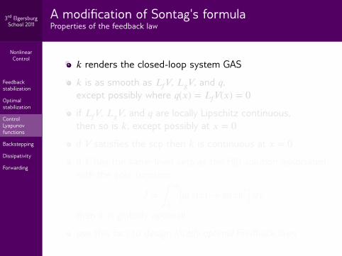
NonlinearControl
Feedbackstabilization
Optimalstabilization
ControlLyapunovfunctions
Backstepping
Dissipativity
Forwarding
3rd ElgersburgSchool 2011
A modification of Sontag's formulaProperties of the feedback law
𝑘 renders the closed-loop system GAS
𝑘 is as smooth as 𝐿𝑓𝑉, 𝐿𝑔𝑉, and 𝑞,except possibly where 𝑞(𝑥) = 𝐿𝑓𝑉(𝑥) = 0
if 𝐿𝑓𝑉, 𝐿𝑔𝑉, and 𝑞 are locally Lipschitz continuous,then so is 𝑘, except possibly at 𝑥 = 0
if 𝑉 satisfies the scp then 𝑘 is continuous at 𝑥 = 0
if 𝑉 has the same level sets as the HJB solution associatedwith the cost function
𝐽 = ∫∞
0[𝑞(𝑥(𝜏)) + |𝑢(𝜏)|2] 𝑑𝜏
then 𝑘 is globally optimal!
use this fact to design locally optimal feedback laws
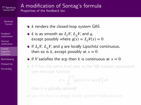
NonlinearControl
Feedbackstabilization
Optimalstabilization
ControlLyapunovfunctions
Backstepping
Dissipativity
Forwarding
3rd ElgersburgSchool 2011 Outline
13 Feedback stabilization
14 Optimal stabilization
15 Control Lyapunov functions
16 Backstepping
17 Dissipativity
18 Forwarding

NonlinearControl
Feedbackstabilization
Optimalstabilization
ControlLyapunovfunctions
Backstepping
Dissipativity
Forwarding
3rd ElgersburgSchool 2011
Backstepping: adding an integratorConstructing a CLF for an extended system
Suppose the system is feedback equivalent to
��1 = 𝐹(𝑥1, 𝑥2) 𝑥1 ∈ ℝ𝑛−𝑚 𝐹(0, 0) = 0��2 = 𝑢 𝑥2, 𝑢 ∈ ℝ𝑚 𝐹 ∈ C1
Suppose we can stabilize the reduced system
��1 = 𝐹(𝑥1, 𝑣) 𝑣 = virtual control
with a 𝐶1, proper, positive definite Lyapunov function 𝑉1(𝑥)and a 𝐶1 feedback law 𝑣 = 𝑘(𝑥1) with 𝑘(0) = 0 such that
𝐷𝑉1(𝑥1) ·𝐹(𝑥1, 𝑘(𝑥1)) < 0 for 𝑥1 ≠ 0
Then we can construct a CLF for the full system …

NonlinearControl
Feedbackstabilization
Optimalstabilization
ControlLyapunovfunctions
Backstepping
Dissipativity
Forwarding
3rd ElgersburgSchool 2011 A CLF for the full system
A simple choice
𝑉2(𝑥1, 𝑥2) = 𝑉1(𝑥1) + ||𝑥2 − 𝑘(𝑥1)||2
A more flexible choice (but not the most flexible)
𝑉2(𝑥1, 𝑥2) = ∫𝑉1(𝑥1)
0𝛾(𝑟) 𝑑𝑟 + (𝑥2 − 𝑘(𝑥1))𝑇 Γ(𝑥1)(𝑥2 − 𝑘(𝑥1))
𝛾 ∶ [0, ∞) → [0, ∞) is C0 with 𝛾(𝑟) > 0 for 𝑟 > 0and ∫ ∞
0 𝛾(𝑟) 𝑑𝑟 = ∞ (simple choice 𝛾 ≡ 1)
Γ is C1 with Γ(𝑥1) = Γ𝑇(𝑥1) > 0 ∀𝑥1 (simple choice Γ ≡ 𝐼)
this makes 𝑉2 a C1, positive definite, and proper function
now verify the CLF property …

NonlinearControl
Feedbackstabilization
Optimalstabilization
ControlLyapunovfunctions
Backstepping
Dissipativity
Forwarding
3rd ElgersburgSchool 2011 Verifying the CLF property
We compute
𝑉2 = 𝛾(𝑉1(𝑥1)) · 𝐷𝑉1(𝑥1) ·𝐹(𝑥1, 𝑥2)
+ (𝑥2 − 𝑘(𝑥1))𝑇 ⟨𝐷Γ(𝑥1), 𝐹(𝑥1, 𝑥2)⟩(𝑥2 − 𝑘(𝑥1))
+ 2(𝑥2 − 𝑘(𝑥1))𝑇 Γ(𝑥1)⏟⏟⏟⏟⏟⏟⏟⏟⏟⏟⏟⏟⏟⏟⏟⏟⏟⏟⏟⏟⏟⏟⏟⏟⏟⏟⏟⏟⏟⏟⏟⏟⏟
𝐿𝑔𝑉2(𝑥1,𝑥2)
[𝑢 − 𝐷𝑘(𝑥1) ·𝐹(𝑥1, 𝑥2)]
If 𝐿𝑔𝑉2(𝑥1, 𝑥2) = 0 then 𝑥2 = 𝑘(𝑥1) and
𝑉2 = 𝛾(𝑉1(𝑥1)) · 𝐷𝑉1(𝑥1) ·𝐹(𝑥1, 𝑘(𝑥1)) < 0 for 𝑥1 ≠ 0
Furthermore, 𝑉2 satisfies the scp, so there is a C0 globallystabilizing feedback (e.g., from Sontag's formula).
If all data are smooth, then there is a smooth feedback.

NonlinearControl
Feedbackstabilization
Optimalstabilization
ControlLyapunovfunctions
Backstepping
Dissipativity
Forwarding
3rd ElgersburgSchool 2011
Backstepping exampleChoosing a virtual feedback
System with 𝑋 = ℝ2 and 𝑢 ∈ ℝ
��1 = 𝑥31 + (𝑥2
1 + 𝑥2)3
��2 = 𝑢
unstable (with finite escape times) when 𝑢 = 0
the linear approximation about 𝑥 = 0 is not stabilizable
Replace 𝑥2 with a virtual control 𝑣 in the 𝑥1-subsystem
��1 = 𝑥31 + (𝑥2
1 + 𝑣)3
𝑣 = 𝑘(𝑥1) = −2𝑥1 − 𝑥21 yields the GAS system ��1 = −7𝑥3
1with Lyapunov function 𝑉(𝑥1) = 𝑥2
1

NonlinearControl
Feedbackstabilization
Optimalstabilization
ControlLyapunovfunctions
Backstepping
Dissipativity
Forwarding
3rd ElgersburgSchool 2011
Backstepping exampleConstructing a CLF
A simple choice
𝑉2(𝑥1, 𝑥2) = 𝑉1(𝑥1) + (𝑥2 − 𝑘(𝑥1))2 = 𝑥21 + (𝑥2 + 2𝑥1 + 𝑥2
1)2
we can use Sontag's formula, or
there are polynomial feedback laws that render 𝑉2 < 0
What about performance?there are many choices for the virtual control law
there are many choices for the CLF
there are many choices for the stabilizing feedback
An open challengeHow do we exploit these design flexibilities to achieve goodclosed-loop performance?

NonlinearControl
Feedbackstabilization
Optimalstabilization
ControlLyapunovfunctions
Backstepping
Dissipativity
Forwarding
3rd ElgersburgSchool 2011
Should we choose an optimal virtual control law?Not necessarily
Apply backstepping to the linear system
��1 = −2𝑥1 + 𝑥2 (virtual subsystem ��1 = −2𝑥1 + 𝑣)��2 = −2𝑥1 + 𝑢
a linear virtual control law 𝑣 = −𝑐𝑥1 leads to a quadraticbackstepping CLF of the form
𝑉2(𝑥1, 𝑥2) = 𝑎𝑥21 + 𝑏(𝑥2 + 𝑐𝑥1)2
for positive 𝑎 and 𝑏
the value function for the cost 𝐽 = ∫ ∞0 (𝑥2
1 + 𝑥22 + 𝑢2) 𝑑𝜏
is of the same quadratic form with 𝑐 = −0.29
the best choice for the virtual control is 𝑣 = 0.29𝑥1, whichis not optimal for the virtual subsystem for any cost thatpenalizes both 𝑥1 and 𝑣 !

NonlinearControl
Feedbackstabilization
Optimalstabilization
ControlLyapunovfunctions
Backstepping
Dissipativity
Forwarding
3rd ElgersburgSchool 2011
Nonlinear dampingHandling unmeasured disturbances
System with 𝑢 ∈ ℝ𝑚 and matched disturbance input 𝑑(𝑡) ∈ ℝ𝑞
�� = 𝑓(𝑥) + 𝑔(𝑥)[𝑢 + 𝑆(𝑥)𝑑] 𝑆(𝑥) ∈ ℝ𝑚×𝑞
suppose we know a CLF 𝑉(𝑥) with an associated stabilizingfeedback law 𝑘(𝑥) for the system with 𝑑 ≡ 0:
𝐿𝑓𝑉(𝑥) + 𝐿𝑔𝑉(𝑥)𝑘(𝑥) < 0 for 𝑥 ≠ 0
assume 𝐿𝑓𝑉(𝑥) + 𝐿𝑔𝑉(𝑥)𝑘(𝑥) ⩽ −𝛼(|𝑥|) for some 𝛼 ∈ 𭒦∞(if this is not the case, we can make it so by replacing 𝑉with 𝜌(𝑉 ) for an appropriate class-𭒦∞ function 𝜌)
add nonlinear damping to the feedback law:
𝑢 = 𝑘(𝑥) − 𝑐𝑆(𝑥)𝑆 𝑇(𝑥)[𝐿𝑔𝑉(𝑥)]𝑇
⏟⏟⏟⏟⏟⏟⏟⏟⏟⏟⏟⏟⏟⏟⏟⏟⏟⏟⏟⏟⏟⏟⏟⏟⏟⏟⏟⏟⏟⏟⏟⏟⏟⏟⏟⏟⏟⏟⏟⏟⏟nonlinear damping
𝑐 > 0

NonlinearControl
Feedbackstabilization
Optimalstabilization
ControlLyapunovfunctions
Backstepping
Dissipativity
Forwarding
3rd ElgersburgSchool 2011 What does nonlinear damping accomplish?
The new Lyapunov derivative becomes
𝑉 = 𝐿𝑓𝑉(𝑥) + 𝐿𝑔𝑉(𝑥)𝑘(𝑥) − 𝑐||𝐿𝑔𝑉(𝑥)𝑆(𝑥)||2 + 𝐿𝑔𝑉(𝑥)𝑆(𝑥)𝑑
⩽ 𝐿𝑓𝑉(𝑥) + 𝐿𝑔𝑉(𝑥)𝑘(𝑥)⏟⏟⏟⏟⏟⏟⏟⏟⏟⏟⏟⏟⏟⏟⏟⏟⏟⏟⏟⏟⏟⏟⏟⏟⏟⏟⏟⏟⏟⏟⏟⏟⏟⏟⏟
⩽−𝛼(|𝑥|)
+ 14𝑐 |𝑑|2 (Young's inequality)
Therefore the closed-loop system is ISS with respect to 𝑑(𝑡).
Nonlinear damping generates ISS systemsAdding a nonlinear damping term to a stabilizing feedback lawwill render the closed-loop system ISS with respect to amatched disturbance.
What if the disturbance is not matched with the control input?

NonlinearControl
Feedbackstabilization
Optimalstabilization
ControlLyapunovfunctions
Backstepping
Dissipativity
Forwarding
3rd ElgersburgSchool 2011
Backstepping with nonlinear dampingAchieving ISS with respect to unmatched disturbances
Example with 𝑋 = ℝ2, 𝑢 ∈ ℝ, 𝑑 ∈ ℝ2
��1 = 𝑥2 + 𝑥21𝑑1 (virtual subsystem ��1 = 𝑣 + 𝑥2
1𝑑1)��2 = 𝑢 + 𝑥1𝑥2𝑑2
Choose 𝑉1(𝑥1) = 𝑥21 and design 𝑣 for the virtual subsystem:
𝑣 = −𝑥1 − 𝑥51⏟⏟⏟
nonlinear damping
𝑉1||𝑥2=𝑣 ⩽ −2𝑥21 + 1
2 𝑑21
Now make a simple choice for the CLF 𝑉2:
𝑉2(𝑥) = 𝑉1(𝑥1) + (𝑥2 + 𝑥1 + 𝑥51)
2
𝑉2 = 𝑉1||𝑥2=𝑣 + 2𝑥1(𝑥2 + 𝑥1 + 𝑥51)
+ 2(𝑥2 + 𝑥1 + 𝑥51)[𝑢 + 𝑥1𝑥2𝑑2 + (1 + 5𝑥4
1)(𝑥2 + 𝑥21𝑑1)]

NonlinearControl
Feedbackstabilization
Optimalstabilization
ControlLyapunovfunctions
Backstepping
Dissipativity
Forwarding
3rd ElgersburgSchool 2011
Backstepping with nonlinear dampingExample continued
To simplify, first choose
𝑢 = −𝑥1 − (1 + 5𝑥41)𝑥2 − (𝑥2 + 𝑥1 + 𝑥5
1) + 𝑢nd
𝑢nd = nonlinear damping term to be designed
and plug in to obtain𝑉2 ⩽ −2𝑉2(𝑥) + 1
2 𝑑21
+ 2(𝑥2 + 𝑥1 + 𝑥51)⏟⏟⏟⏟⏟⏟⏟⏟⏟⏟⏟⏟⏟⏟⏟⏟⏟⏟⏟⏟⏟⏟⏟⏟⏟
𝐿𝑔𝑉2(𝑥)
[𝑢nd + [(1 + 5𝑥41)𝑥2
1 𝑥1𝑥2]⏟⏟⏟⏟⏟⏟⏟⏟⏟⏟⏟⏟⏟⏟⏟⏟⏟⏟⏟⏟⏟⏟⏟⏟⏟⏟⏟⏟⏟⏟⏟⏟⏟⏟⏟𝑆(𝑥)
𝑑]
Choose 𝑢nd = − 𝑐𝑆(𝑥)𝑆 𝑇(𝑥)𝐿𝑔𝑉2(𝑥) (with 𝑥171 !!) to obtain
𝑉2 ⩽ −2𝑉2(𝑥) + 12 𝑑2
1 + 14𝑐 (𝑑2
1 + 𝑑22)
The closed-loop system is ISS with respect to 𝑑 = (𝑑1, 𝑑2).
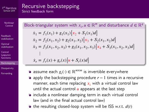
NonlinearControl
Feedbackstabilization
Optimalstabilization
ControlLyapunovfunctions
Backstepping
Dissipativity
Forwarding
3rd ElgersburgSchool 2011
Recursive backsteppingStrict feedback form
Block-triangular system with 𝑥𝑖, 𝑢 ∈ ℝ𝑚 and disturbance 𝑑 ∈ ℝ𝑞
��1 = 𝑓1(𝑥1) + 𝑔1(𝑥1)[𝑥2 + 𝑆1(𝑥1)𝑑]��2 = 𝑓2(𝑥1, 𝑥2) + 𝑔2(𝑥1, 𝑥2)[𝑥3 + 𝑆2(𝑥1, 𝑥2)𝑑]��3 = 𝑓3(𝑥1, 𝑥2, 𝑥3) + 𝑔3(𝑥1, 𝑥2, 𝑥3)[𝑥4 + 𝑆3(𝑥1, 𝑥2, 𝑥3)𝑑]
⋮��𝑟 = 𝑓𝑟(𝑥) + 𝑔𝑟(𝑥)[𝑢 + 𝑆𝑟(𝑥)𝑑]
assume each 𝑔𝑖(·) ∈ ℝ𝑚×𝑚 is invertible everywhereapply the backstepping procedure 𝑟 − 1 times in a recursivemanner, each time replacing 𝑥𝑖 with a virtual control lawuntil the actual control 𝑢 appears at the last stepinclude a nonlinear damping term in each virtual controllaw (and in the final actual control law)the resulting closed-loop system will be ISS w.r.t. 𝑑(𝑡)

NonlinearControl
Feedbackstabilization
Optimalstabilization
ControlLyapunovfunctions
Backstepping
Dissipativity
Forwarding
3rd ElgersburgSchool 2011 Outline
13 Feedback stabilization
14 Optimal stabilization
15 Control Lyapunov functions
16 Backstepping
17 Dissipativity
18 Forwarding

NonlinearControl
Feedbackstabilization
Optimalstabilization
ControlLyapunovfunctions
Backstepping
Dissipativity
Forwarding
3rd ElgersburgSchool 2011
DissipativityGeneral concepts
In a nutshella dissipative system cannot produce
an infinite amount of work,—OR—
the change in its internal energynever exceeds the work done on it
Key pointEnergy and work are abstractly defined and may have norelation to physical quantities …

NonlinearControl
Feedbackstabilization
Optimalstabilization
ControlLyapunovfunctions
Backstepping
Dissipativity
Forwarding
3rd ElgersburgSchool 2011 Classical dissipativity
Given:a system with state 𝑥(𝑡), input 𝑢(𝑡), and output 𝑦(𝑡)a supply rate 𝜔(𝑢, 𝑦, 𝑡)
Available storage 𝜑𝑎
𝜑𝑎(𝑥0, 𝑡0) = − inf ∫𝑡
𝑡0
𝜔(𝑢(𝜏), 𝑦(𝜏), 𝜏) 𝑑𝜏
where the infimum is taken over all 𝑡 ⩾ 𝑡0 and all systemtrajectories having state 𝑥0 at time 𝑡0
DefinitionThe system is dissipative with respect to 𝜔 when
𝜑𝑎(𝑥0, 𝑡0) < ∞ for all 𝑥0 and 𝑡0

NonlinearControl
Feedbackstabilization
Optimalstabilization
ControlLyapunovfunctions
Backstepping
Dissipativity
Forwarding
3rd ElgersburgSchool 2011 Dissipation inequality
TheoremA system is dissipative if and only if there is a nonnegativestorage function 𝑉 which satisfies the dissipation inequality
𝑉(𝑥(𝑡), 𝑡)⏟⏟⏟⏟⏟⏟⏟⏟⏟
current energy
⩽ 𝑉(𝑥(𝑡0), 𝑡0)⏟⏟⏟⏟⏟⏟⏟⏟⏟⏟⏟⏟⏟initial energy
+ ∫𝑡
𝑡0
𝜔(𝑢(𝜏), 𝑦(𝜏), 𝜏) 𝑑𝜏⏟⏟⏟⏟⏟⏟⏟⏟⏟⏟⏟⏟⏟⏟⏟⏟⏟⏟⏟⏟⏟⏟⏟⏟⏟⏟⏟⏟⏟⏟⏟⏟⏟⏟⏟⏟⏟
work done on system
along all system trajectories for all 𝑡 ⩾ 𝑡0.
In a dissipative system, the available storage 𝜑𝑎 is a storagefunction which bounds every other storage function from below.
Differential version: 𝑉(𝑡) ⩽ 𝜔(𝑢, 𝑦, 𝑡)

NonlinearControl
Feedbackstabilization
Optimalstabilization
ControlLyapunovfunctions
Backstepping
Dissipativity
Forwarding
3rd ElgersburgSchool 2011 System properties characterized by dissipativity
Classical properties:passivity: 𝜔 = 𝑦𝑇𝑢
ℒ𝑝-gain: 𝜔 = 𝛾𝑝|𝑢|𝑝 − |𝑦|𝑝 (1 ⩽ 𝑝 < ∞)
output strict passivity: 𝜔 = 𝑦𝑇𝑢 − |𝑦|2 (implies ℒ2-gain)
input strict passivity: 𝜔 = 𝑦𝑇𝑢 − 𝛿|𝑢|2
More recent connections to dissipativity:ISS and iISS
minimum-phase property
ℓ∞-gain for discrete-time systems
NonlinearControl
Feedbackstabilization
Optimalstabilization
ControlLyapunovfunctions
Backstepping
Dissipativity
Forwarding
3rd ElgersburgSchool 2011 Why is dissipativity useful?
Divide and conquerThe interconnection of dissipative systems with complementarysupply rates is again dissipative!
Classical examples:small-gain theorem: if two systems have ℒ𝑝-gains whoseproduct is less than one, then their feedbackinterconnection is stablepassivity theorem: the negative feedbackinterconnection of passive systems is stable/passive

NonlinearControl
Feedbackstabilization
Optimalstabilization
ControlLyapunovfunctions
Backstepping
Dissipativity
Forwarding
3rd ElgersburgSchool 2011
An example of a passive systemA robot manipulator
Dynamics of a robot manipulator
𝑀(𝑞) 𝑞 + 𝐶(𝑞, 𝑞) 𝑞 + 𝑔(𝑞) = 𝜏
𝑞 is the vector of configuration variables𝜏 is the vector of applied joint torques𝑀(𝑞) is the mass matrix𝐶(𝑞, 𝑞) characterizes the Coriolis and centrifugal forces𝑔(𝑞) represents the gravitational forces
Model properties:𝑔(·) is the gradient of a potential field:
𝑔𝑇(𝑞) = 𝐷𝐺(𝑞) for some nonnegative gravity field 𝐺(𝑞)𝑞𝑇[��(𝑞, 𝑞) − 2𝐶(𝑞, 𝑞)] 𝑞 ≡ 0 (fictitious forces do no work)

NonlinearControl
Feedbackstabilization
Optimalstabilization
ControlLyapunovfunctions
Backstepping
Dissipativity
Forwarding
3rd ElgersburgSchool 2011 A storage function for the robot manipulator
Look at total energy as a candidate storage function
𝑉(𝑞, 𝑞) = 12 𝑞𝑇𝑀(𝑞) 𝑞⏟⏟⏟⏟⏟⏟⏟⏟⏟⏟⏟
kinetic
+ 𝐺(𝑞)⏟⏟⏟
potential
This storage function satisfies𝑉 = 𝑞𝑇𝜏
and thus the system is passive from the applied torques 𝑢 = 𝜏to the joint velocities 𝑦 = 𝑞.
This passivity is the basis for many robot control strategies.
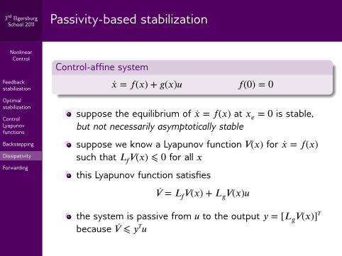
NonlinearControl
Feedbackstabilization
Optimalstabilization
ControlLyapunovfunctions
Backstepping
Dissipativity
Forwarding
3rd ElgersburgSchool 2011 Passivity-based stabilization
Control-affine system
�� = 𝑓(𝑥) + 𝑔(𝑥)𝑢 𝑓(0) = 0
suppose the equilibrium of �� = 𝑓(𝑥) at 𝑥𝑒 = 0 is stable,but not necessarily asymptotically stable
suppose we know a Lyapunov function 𝑉(𝑥) for �� = 𝑓(𝑥)such that 𝐿𝑓𝑉(𝑥) ⩽ 0 for all 𝑥
this Lyapunov function satisfies𝑉 = 𝐿𝑓𝑉(𝑥) + 𝐿𝑔𝑉(𝑥)𝑢
the system is passive from 𝑢 to the output 𝑦 = [𝐿𝑔𝑉(𝑥)]𝑇
because 𝑉 ⩽ 𝑦𝑇𝑢

NonlinearControl
Feedbackstabilization
Optimalstabilization
ControlLyapunovfunctions
Backstepping
Dissipativity
Forwarding
3rd ElgersburgSchool 2011
Passivity-based stabilizationUsing LaSalle's theorem to prove asymptotic stability
Choose 𝑢 = −𝜎(𝑦) where 𝑦𝑇𝜎(𝑦) is positive definite in 𝑦:
𝑉 = 𝐿𝑓𝑉(𝑥) − 𝑦𝑇𝜎(𝑦)
(for example, 𝑢 = −𝐾𝑦 for 𝐾 > 0). Then 𝑥 converges to thelargest invariant set contained in the set
{𝑥 ∈ 𝑋 ∶ 𝐿𝑓𝑉(𝑥) = 𝐿𝑔𝑉(𝑥) = 0}
if this largest invariant set contains just the equilibrium𝑥𝑒 = 0, then we have asymptotic stability
this will hold in particular when the system �� = 𝑓(𝑥) iszero-state observable through the output 𝑦 = [𝐿𝑔𝑉(𝑥)]𝑇

NonlinearControl
Feedbackstabilization
Optimalstabilization
ControlLyapunovfunctions
Backstepping
Dissipativity
Forwarding
3rd ElgersburgSchool 2011 Feedback passivation
Suppose a system is feedback equivalent to the cascade
��1 = 𝑓(𝑥1) + 𝑔(𝑥1)𝑥2 𝑓(0) = 0��2 = 𝑢
suppose we know a Lyapunov function 𝑉1(𝑥1) for��1 = 𝑓(𝑥1) such that 𝐿𝑓𝑉1(𝑥1) ⩽ 0 for all 𝑥1
the system has relative degree (1, …, 1) and isweakly minimum-phase with respect to the output 𝑦 = 𝑥2
consider 𝑉2(𝑥1, 𝑥2) = 𝑉1(𝑥1) + 12 |𝑦|2 with derivative
𝑉2 = 𝐿𝑓𝑉1(𝑥1) + 𝐿𝑔𝑉1(𝑥1)𝑦 + 𝑦𝑇𝑢
choose 𝑢 = −[𝐿𝑔𝑉1(𝑥1)]𝑇 + 𝑣 for a new input 𝑣:𝑉2 = 𝐿𝑓𝑉1(𝑥1) + 𝑦𝑇𝑣
passivity from 𝑣 to 𝑦, stabilization 𝑣 = −𝜎(𝑦) as before

NonlinearControl
Feedbackstabilization
Optimalstabilization
ControlLyapunovfunctions
Backstepping
Dissipativity
Forwarding
3rd ElgersburgSchool 2011
Feedback passivationExample
Cascade system, relative degree 1 and weakly minimum-phase
��1 = −𝑥2 + 𝑥21𝑥3
��2 = 𝑥1 + 𝑥1𝑥2𝑥3
��3 = 𝑢 𝑦 = 𝑥3
choose 𝑉1(𝑥1, 𝑥2) = 𝑥21 + 𝑥2
2 so that 𝐿𝑓𝑉1(𝑥1, 𝑥2) ≡ 0
then 𝐿𝑔𝑉1(𝑥1, 𝑥2) = 2𝑥1(𝑥21 + 𝑥2
2)
choose 𝑢 = −𝐿𝑔𝑉1(𝑥1, 𝑥2) − 𝑦 = −2𝑥1(𝑥21 + 𝑥2
2) − 𝑥3
asymptotic stability because 𝑦 ≡ 0 implies 𝑢 ≡ 0 implies𝐿𝑔𝑉1(𝑥1, 𝑥2) ≡ 0 implies 𝑥1 ≡ 𝑥2 ≡ 0 (then use LaSalle)

NonlinearControl
Feedbackstabilization
Optimalstabilization
ControlLyapunovfunctions
Backstepping
Dissipativity
Forwarding
3rd ElgersburgSchool 2011 Outline
13 Feedback stabilization
14 Optimal stabilization
15 Control Lyapunov functions
16 Backstepping
17 Dissipativity
18 Forwarding

NonlinearControl
Feedbackstabilization
Optimalstabilization
ControlLyapunovfunctions
Backstepping
Dissipativity
Forwarding
3rd ElgersburgSchool 2011 Finding a Lyapunov function for passivity design
Example with 𝑋 = ℝ2 and 𝑢 ∈ ℝ
��1 = 𝑥2 − 𝑥22 + 𝑥2
1𝑢��2 = −𝑥2 + 𝑢
with 𝑢 = 0, the equilibrium 𝑥𝑒 = 0 is stablebut not asymptotically stable
to perform passivity-based stabilization,we need to know 𝑉(𝑥) such that 𝐿𝑓𝑉(𝑥) ⩽ 0
propose a candidate 𝑉(𝑥) of the form
𝑉(𝑥) = 𝑥21 + Ψ(𝑥1, 𝑥2) + 𝑥2
2
what should the cross term Ψ(𝑥1, 𝑥2) be?

NonlinearControl
Feedbackstabilization
Optimalstabilization
ControlLyapunovfunctions
Backstepping
Dissipativity
Forwarding
3rd ElgersburgSchool 2011 Defining the cross term
when 𝑢 = 0 we have𝑉 = 𝐿𝑓𝑉(𝑥) = 2𝑥1(𝑥2 − 𝑥2
2) + Ψ − 2𝑥22
if Ψ = −2𝑥1(𝑥2 − 𝑥22) then 𝐿𝑓𝑉(𝑥) = −2𝑥2
2 ⩽ 0
thus choose
Ψ(𝑥1, 𝑥2) = Ψ(𝑥) =∫∞
02𝜑1(𝜏, 𝑥)[𝜑2(𝜏, 𝑥) − 𝜑2
2(𝜏, 𝑥)] 𝑑𝜏
where 𝜑(𝑡, 𝑥) = (𝜑1, 𝜑2) denotes the flow of 𝑓
we can find 𝜑(𝑡, 𝑥) and Ψ(𝑥) in closed form:
Ψ(𝑥1, 𝑥2) = 𝑥1(2𝑥2 − 𝑥22) + 𝑥2
2 − 𝑥32 + 1
4 𝑥42
the resulting 𝑉(𝑥) is positive definite and proper,and we proceed with the passivity design …
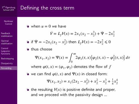

NonlinearControl
Feedbackstabilization
Optimalstabilization
ControlLyapunovfunctions
Backstepping
Dissipativity
Forwarding
3rd ElgersburgSchool 2011
Finishing the controller designBounded control with arbitrarily small bound
Now we compute the passive output 𝑦 = 𝐿𝑔𝑉(𝑥):
𝐿𝑔𝑉(𝑥) = 2𝑥1 + 4𝑥2 − 2𝑥1𝑥2 − 3𝑥22 + 2𝑥3
1 + 2𝑥21𝑥2 + 𝑥3
2 − 𝑥21𝑥2
2
For a bounded control we can choose
𝑢 = 𝑘(𝑥1, 𝑥2) = − tanh(1𝜀 𝐿𝑔𝑉(𝑥)) for any > 0
Finally, confirm that the equilibrium 𝑥𝑒 = 0 is the largestinvariant set satisfying 𝐿𝑓𝑉(𝑥) ≡ 𝐿𝑔𝑉(𝑥) ≡ 0 (yes, because𝐿𝑓𝑉(𝑥) = −2𝑥2
2 which means 𝑥2 ≡ 0 which means𝐿𝑔𝑉(𝑥) = 2𝑥1(1 + 𝑥2
1) ≡ 0 which means 𝑥1 ≡ 0).
The closed-loop system is GAS and locally exponentially stable(the linearization at 𝑥𝑒 = 0 is �� = 𝐴𝑥 with a Hurwitz 𝐴).

NonlinearControl
Feedbackstabilization
Optimalstabilization
ControlLyapunovfunctions
Backstepping
Dissipativity
Forwarding
3rd ElgersburgSchool 2011
Forwarding: adding another partRepeating the passivity design for the new system
Add a third state 𝑥0 ∈ ℝ
��0 = 𝑓(𝑥0, 𝑥1, 𝑥2) + 𝑔(𝑥0, 𝑥1, 𝑥2)𝑢 𝑓(𝑥0, 0, 0) ≡ 0��1 = 𝑥2 − 𝑥2
2 + 𝑥21𝑢 𝑓, 𝑔 glob. Lip. in 𝑥0
��2 = −𝑥2 + 𝑢
add a new term to the controller, 𝑢 = 𝑘(𝑥1, 𝑥2) + 𝑣when 𝑣 = 0, the equilibrium 𝑥𝑒 = 0 is stablebut not asymptotically stable, just like beforepropose a candidate Lyapunov function 𝑉0 of the form
𝑉0(𝑥0, 𝑥1, 𝑥2) = 𝑥20 + Ψ0(𝑥0, 𝑥1, 𝑥2) + 𝑉(𝑥1, 𝑥2)
compute the cross term Ψ0 as before (numerically?)apply passivity design for the new control 𝑣to achieve GAS for the new system

NonlinearControl
Unconstrainedcontrol
Constrainedcontrol
3rd ElgersburgSchool 2011
Part IV
Optimal control

NonlinearControl
Unconstrainedcontrol
Constrainedcontrol
3rd ElgersburgSchool 2011
Finite-horizon optimal controlCost function
System with finite-horizon cost function
�� = 𝑓(𝑥, 𝑢) 𝑥(0) = 𝑥0
𝐽(𝑥0, 𝑢(·)) = 𝜑(𝑥(𝑡𝑓)) + ∫𝑡𝑓
0𝐿(𝑥(𝜏), 𝑢(𝜏)) 𝑑𝜏
𝜑 is the terminal cost(the penalty on the the state 𝑥(𝑡𝑓) at the final time 𝑡𝑓)
𝐿 is the Lagrangian cost
assume 𝑓, 𝜑, and 𝐿 are C1, and assume 𝑥0 and 𝑡𝑓 are fixed
GoalDerive necessary conditions for an open-loop control 𝑢(𝑡) tominimize the cost over all possible controls.

NonlinearControl
Unconstrainedcontrol
Constrainedcontrol
3rd ElgersburgSchool 2011 Outline
19 Unconstrained control
20 Constrained control
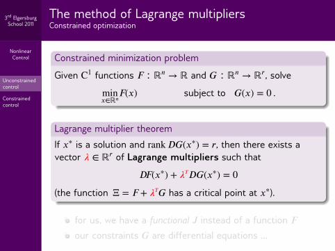
NonlinearControl
Unconstrainedcontrol
Constrainedcontrol
3rd ElgersburgSchool 2011
The method of Lagrange multipliersConstrained optimization
Constrained minimization problem
Given C1 functions 𝐹 ∶ ℝ𝑛 → ℝ and 𝐺 ∶ ℝ𝑛 → ℝ𝑟, solve
min𝑥∈ℝ𝑛
𝐹(𝑥) subject to 𝐺(𝑥) = 0 .
Lagrange multiplier theorem
If 𝑥∗ is a solution and rank 𝐷𝐺(𝑥∗) = 𝑟, then there exists avector 𝜆 ∈ ℝ𝑟 of Lagrange multipliers such that
𝐷𝐹(𝑥∗) + 𝜆𝑇𝐷𝐺(𝑥∗) = 0
(the function Ξ = 𝐹 + 𝜆𝑇𝐺 has a critical point at 𝑥∗).
for us, we have a functional 𝐽 instead of a function 𝐹our constraints 𝐺 are differential equations …

NonlinearControl
Unconstrainedcontrol
Constrainedcontrol
3rd ElgersburgSchool 2011
Adding a time-varying Lagrange multiplierAn informal derivation
The augmented cost Ξ with Lagrange multiplier 𝜆(𝑡) ∈ ℝ𝑛
Ξ = 𝜑(𝑥(𝑡𝑓)) + ∫𝑡𝑓
0[𝐿(𝑥(𝜏), 𝑢(𝜏)) + 𝜆𝑇(𝜏)(𝑓(𝑥(𝜏), 𝑢(𝜏)) − ��(𝜏))]𝑑𝜏
The Hamiltonian
𝐻(𝑥, 𝑢, 𝜆) = 𝐿(𝑥, 𝑢) + 𝜆𝑇𝑓(𝑥, 𝑢)
Integrate by parts to get
Ξ = 𝜑(𝑥(𝑡𝑓)) + ∫𝑡𝑓
0[𝐻(𝑥(𝜏), 𝑢(𝜏), 𝜆(𝜏)) + 𝜆𝑇(𝜏)𝑥(𝜏)]𝑑𝜏
+ 𝜆𝑇(0)𝑥0 − 𝜆𝑇(𝑡𝑓)𝑥(𝑡𝑓)
Now set derivatives of Ξ with respect to 𝑥 and 𝑢 to zero …

NonlinearControl
Unconstrainedcontrol
Constrainedcontrol
3rd ElgersburgSchool 2011 The derivative with respect to 𝑥(𝑡)
Informally,
𝜕Ξ𝜕𝑥
= ∫𝑡𝑓
0[
𝜕𝐻𝜕𝑥
(𝑥(𝜏), 𝑢(𝜏), 𝜆(𝜏)) + 𝜆𝑇(𝜏)]𝑑𝜏
To make this zero, we set
𝜆 = −𝜕𝐻𝑇
𝜕𝑥(𝑥, 𝑢, 𝜆)
If 𝑥(𝑡𝑓) is not specified, then we set
0 = 𝜕Ξ𝜕𝑥(𝑡𝑓)
= 𝐷𝜑(𝑥(𝑡𝑓)) − 𝜆𝑇(𝑡𝑓)
If 𝑥(𝑡𝑓) is free (not specified)
𝜆(𝑡𝑓) = [𝐷𝜑(𝑥(𝑡𝑓))]𝑇

NonlinearControl
Unconstrainedcontrol
Constrainedcontrol
3rd ElgersburgSchool 2011 The derivative with respect to 𝑢(𝑡)
Informally,
𝜕Ξ𝜕𝑢
= ∫𝑡𝑓
0
𝜕𝐻𝜕𝑢
(𝑥(𝜏), 𝑢(𝜏), 𝜆(𝜏)) 𝑑𝜏
This should be zero so we set
𝜕𝐻𝜕𝑢
(𝑥(𝑡), 𝑢(𝑡), 𝜆(𝑡)) = 0 for almost all 𝑡
As a consequence, we observe that
�� = 𝜕𝐻𝜕𝑥
⋅ ��⏟
𝑓(𝑥,𝑢)
+ 𝜕𝐻𝜕𝜆⏟
𝑓𝑇(𝑥,𝑢)
⋅ 𝜆⏟
−𝜕𝐻𝑇/𝜕𝑥
= 0 .
The Hamiltonian is constant under an optimal trajectory.

NonlinearControl
Unconstrainedcontrol
Constrainedcontrol
3rd ElgersburgSchool 2011
Putting it all togetherNecessary conditions for optimality
If 𝑢(𝑡) is an optimal trajectory, then
��(𝑡) = 𝑓(𝑥(𝑡), 𝑢(𝑡)) = 𝜕𝐻𝑇
𝜕𝜆(𝑥(𝑡), 𝑢(𝑡), 𝜆(𝑡))
𝜆(𝑡) = −𝜕𝐻𝑇
𝜕𝑥(𝑥(𝑡), 𝑢(𝑡), 𝜆(𝑡))
0 = 𝜕𝐻𝜕𝑢
(𝑥(𝑡), 𝑢(𝑡), 𝜆(𝑡)) for almost all 𝑡
Boundary conditions if 𝑥(𝑡𝑓) is free:
𝑥(0) = 𝑥0 𝜆(𝑡𝑓) = [𝐷𝜑(𝑥(𝑡𝑓))]𝑇
Boundary conditions if 𝑥(𝑡𝑓) is specified:
𝑥(0) = 𝑥0 𝑥(𝑡𝑓) = 𝑥𝑓

NonlinearControl
Unconstrainedcontrol
Constrainedcontrol
3rd ElgersburgSchool 2011 Computing an optimal control
first set 𝜕𝐻/𝜕𝑢 = 0 and solve for 𝑢 in terms of 𝑥 and 𝜆
plug this 𝑢 into the Hamiltonian ODE
��(𝑡) = 𝑓(𝑥(𝑡), 𝑢(𝑡)) = 𝜕𝐻𝑇
𝜕𝜆(𝑥(𝑡), 𝑢(𝑡), 𝜆(𝑡))
𝜆(𝑡) = −𝜕𝐻𝑇
𝜕𝑥(𝑥(𝑡), 𝑢(𝑡), 𝜆(𝑡))
which has mixed boundary conditions at 𝑡 = 0 and 𝑡 = 𝑡𝑓solve the resulting two-point boundary-value problem(in MATLAB you might use bvp4c or bvp5c)
if there are multiple solutions,choose the ones having the smallest cost
use other methods to verify that the solution is optimal(for example, check second derivatives at the solution)

NonlinearControl
Unconstrainedcontrol
Constrainedcontrol
3rd ElgersburgSchool 2011
Computing an optimal controlAn example
Fixed initial and final states with 𝑡𝑓 = 1
��1 = 𝑥22 𝑥(0) = (0, 0)
��2 = 𝑢 𝑥(1) = (1, 0)
𝐽 = ∫1
0𝑢2(𝜏) 𝑑𝜏
𝐻(𝑥, 𝑢, 𝜆) = 𝑢2 + 𝜆1𝑥22 + 𝜆2𝑢 𝜕𝐻
𝜕𝑢= 2𝑢 + 𝜆2
𝑢(𝑡) = − 12 𝜆2(𝑡) 𝜕𝐻
𝜕𝑥= [0 2𝜆1𝑥2]

NonlinearControl
Unconstrainedcontrol
Constrainedcontrol
3rd ElgersburgSchool 2011
Computing an optimal controlAn example
Solve the boundary-value problem
��1 = 𝑥22 𝑥(0) = (0, 0)
��2 = − 12 𝜆2 𝑥(1) = (1, 0)
𝜆1 = 0𝜆2 = −2𝜆1𝑥2
Many solutions:
𝜔 = 𝑘𝜋 , 𝑘 = 1, 2, … 𝜆1(𝑡) ≡ −𝜔2
𝑥1(𝑡) = 𝑡 − 12𝜔 sin(2𝜔𝑡) 𝜆2(𝑡) = ∓𝜔2√2 cos(𝜔𝑡)
𝑥2(𝑡) = ±√2 sin(𝜔𝑡) 𝑢(𝑡) = ±𝜔√2 cos(𝜔𝑡)
The solutions with 𝜔 = 𝜋 have the smallest cost.
NonlinearControl
Unconstrainedcontrol
Constrainedcontrol
3rd ElgersburgSchool 2011 Outline
19 Unconstrained control
20 Constrained control

NonlinearControl
Unconstrainedcontrol
Constrainedcontrol
3rd ElgersburgSchool 2011 The Pontryagin maximum (or minimum) principle
suppose the controls can only take values in 𝒰 ⊂ ℝ𝑚
suppose 𝒰 is not open (e.g., 𝒰 is compact)
then 𝜕𝐻/𝜕𝑢 = 0 is no longer necessaryalong the optimal trajectory
instead we must have
𝐻(𝑥(𝑡), 𝑢(𝑡), 𝜆(𝑡)) = min𝔲∈𝒰
𝐻(𝑥(𝑡), 𝔲, 𝜆(𝑡))
for almost all 𝑡


![Nonlinear control systems[1]](https://img.pdfslide.us/doc/110x75/5561fd91d8b42a25488b507e/nonlinear-control-systems1.jpg)
![[222]Nonlinear Dynamical Control Systems](https://img.pdfslide.us/doc/110x75/563db918550346aa9a99f182/222nonlinear-dynamical-control-systems.jpg)