Nondestructive Inspection of an FRP Composite Tank

Dr. Michael Werner

MTI Project 126-98 Tank T-40, Akzo Nobel Functional Chemicals LLC

Gallipolis Ferry, WV November 27-28, 2001 EXECUTIVE SUMMARY The objective of this effort is to demonstrate nondestructive capabilities for quantitive inspection of Fiber Reinforced Polymeric (FRP) vessels using proprietary microwave sensors. Encouraging results were obtained in an on-site tank inspection performed to test the sensitivity of novel microwave resonator sensors to known liquid-filled blister defects in FRP tanks that have been in hydrochloric acid (HCl) service. At issue was whether the sensor can distinguish, clearly and repeatably without false alarms, a blistered area from a known good area of the tank. The sensor is sensitive to the effective microwave loss factor (ε’’) of whatever admixture of test materials are placed in contact with the sensor. In general, liquid-filled blisters stand out from the rest of an FRP tank because aqueous liquids are very lossy (i.e., large ε’’). However, before the inspection there was concern whether Tank T-40’s blisters could be detected because, although the blisters are quite large, they are located inside the tank wall that is nominally 1½ inch thick, as specified in T-40’s mechanical drawing. The electromagnetic field supported by the sensor is believed to evanesce (i.e. decay exponentially as it penetrates) into the test material; consequently, the more distant an anomaly, the less the anomaly should stand out from the background. Actually, T-40’s blisters proved to be quite visible to the sensor with excellent (40%) signal contrast, in spite of the thick wall and competing variables; among them, an unknown chemical residue on the tank surface. Since all the blisters in this tank were quite large it was not possible to determine the lowest threshold area of blister visibility for the sensor used in the inspection. To learn more, a future inspection should encounter a range of blister sizes to determine the threshold size for a given wall thickness. Further, an ideal test would combine destructive testing with NDT to compare the actual blister distribution with the mapping representation derived from sensor images, and to observe a blister in cross-section. The T-40 test results are in contradistinction to KDC’s first on-site inspection (DuPont, Belle WV) where all the blisters were subthreshold, being quite small in area and had apparently been drained of liquid content while the tank was kept empty.

1

BACKGROUND The resonator sensors are hand held probes, described in a number of previous reports, which are moved by hand along the outer surface of a tank. The equipment package for these initial tests consists of the sensor, a laboratory network analyzer, a five foot cable, and a ruggedized laptop computer. Medium-term equipment development should enable dispensing with the network analyzer and cable. The Akzo Nobel plant in Gallipolis Ferry had two potentially blister-ridden tanks available, both of them outdoors. Of these, one had only been in service for six years and proved upon vessel entry and visual inspection to have smooth featureless internal walls with no blisters whatever. The walls are 3/8 inch thick. The second Akzo Nobel tank, T-40, is contained inside an FRP shell of material, with overall wall thickness specified as 1½ inch. This extreme wall thickness exceeded the known limits of the sensor’s penetration depth by a factor of three. See Photos 1- 3 for external views of this tank.

Photo 1. Akzo Nobel chemical tank T-40 captured in an FRP shell, diameter about five feet, with engineer pointing to the part to be inspected. The internal blisters are located just below the catwalk, where the shell necks down into a narrow cylinder. A man-lift was required to reach the zone to be tested.

2

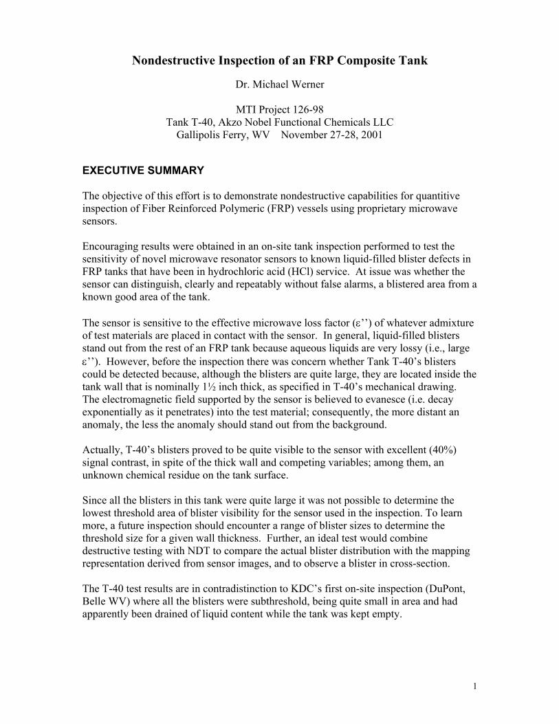
The tank contained aqueous liquid. Using round numbers, the bottom of the tank was about three feet from the ground, then the liquid level was perhaps another three feet above that. Above the liquid level there was about another three feet of vapor and clean unblemished wall. All the blisters were located above that, about nine to ten feet above ground level, at the top of the tank. Above the top of the tank, the shell necks down into a thin cylinder that is perhaps fifteen feet tall. The outer surface of the tank (or shell) is reasonably smooth, only slightly wavy, but increasingly wavy towards the very top end of the blistered region. The surface is encrusted with the tightly-adhering multicolored residue of what appeared to be spills of a number of chemicals the tank has contained over the years. Two Akzo engineers were able to scrape off part of this residue where it had caked up.

Estimated liquid level

Vapor and blisters

liquid

Photo 2. Closeup of Photo 1. The black lines on the tank surface represent internal features. The tank contained liquid up to the lower black line. Although vessel entry into the second tank was not possible as it was in service, an inspection in August, 2001 revealed the presence of several very large liquid-filled delaminations in an FEP lining. In what follows, to be consistent with previous communication we call these delaminations “blisters,” although their shape is reported to be more like a pocket; narrow at the bottom and wide at the top. See photo 4. The thickness of the liquid in each blister is said to increase with height up to some limit.It is not known to the writer whether the blisters were in the tank material or between the tank and the outer shell. This latter possibility might explain the high degree of contrast of the blisters if the shell material is fairly thin.

3

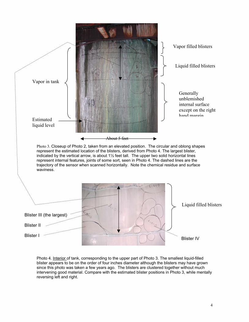
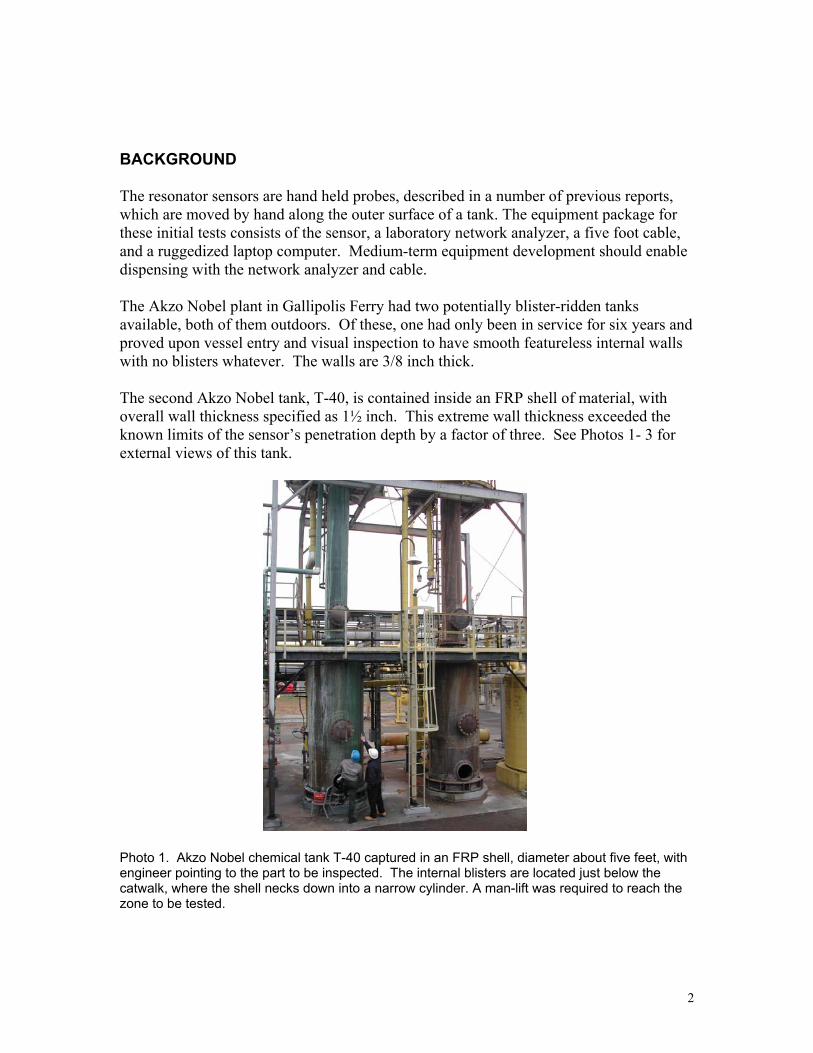
Photo 3. Closeup of Photo 2, taken from an elevated position. The circular andrepresent the estimated location of the blisters, derived from Photo 4. The largindicated by the vertical arrow, is about 1½ feet tall. The upper two solid horizrepresent internal features, joints of some sort, seen in Photo 4. The dashed litrajectory of the sensor when scanned horizontally. Note the chemical residuewaviness.

Liquid filled blisters

Estimated liquid level

Vapor filled blisters

Vapor in tank

About 5 feet

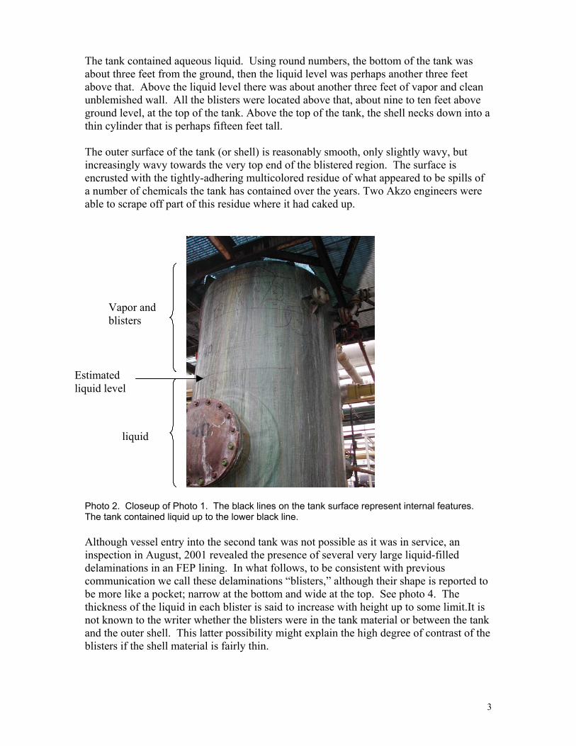
Blister III (the largest) Blister II Blister I

Photo 4. Interior of tank, corresponding to the upper part of Photo 3. The smalblister appears to be on the order of four inches diameter although the blisterssince this photo was taken a few years ago. The blisters are clustered togetheintervening good material. Compare with the estimated blister positions in Phoreversing left and right.

Generally unblemished internal surface except on the right hand margin

oblong shapes est blister, ontal lines nes are the and surface

Liquid filled blisters

Blister IV

lest liquid-filled may have grown r without much to 3, while mentally

4

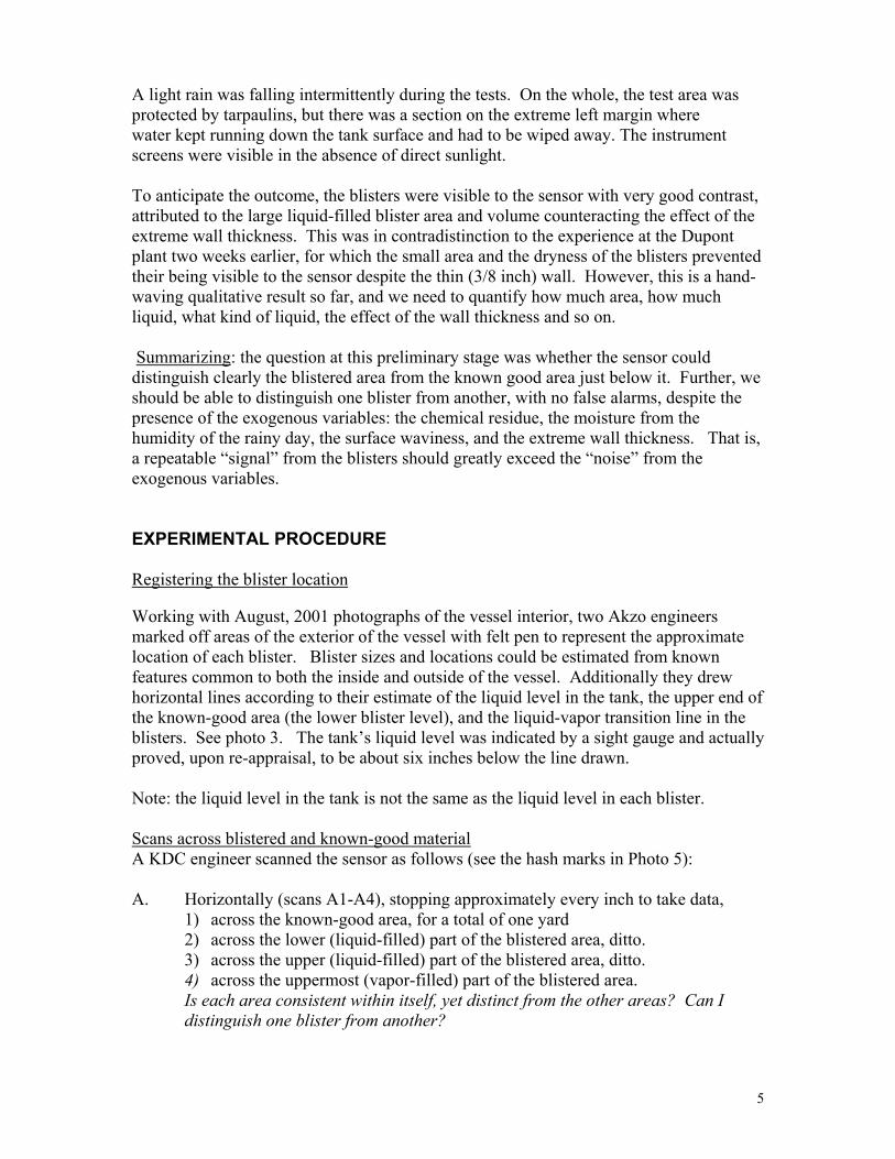
A light rain was falling intermittently during the tests. On the whole, the test area was protected by tarpaulins, but there was a section on the extreme left margin where water kept running down the tank surface and had to be wiped away. The instrument screens were visible in the absence of direct sunlight. To anticipate the outcome, the blisters were visible to the sensor with very good contrast, attributed to the large liquid-filled blister area and volume counteracting the effect of the extreme wall thickness. This was in contradistinction to the experience at the Dupont plant two weeks earlier, for which the small area and the dryness of the blisters prevented their being visible to the sensor despite the thin (3/8 inch) wall. However, this is a hand-waving qualitative result so far, and we need to quantify how much area, how much liquid, what kind of liquid, the effect of the wall thickness and so on. Summarizing: the question at this preliminary stage was whether the sensor could distinguish clearly the blistered area from the known good area just below it. Further, we should be able to distinguish one blister from another, with no false alarms, despite the presence of the exogenous variables: the chemical residue, the moisture from the humidity of the rainy day, the surface waviness, and the extreme wall thickness. That is, a repeatable “signal” from the blisters should greatly exceed the “noise” from the exogenous variables. EXPERIMENTAL PROCEDURE Registering the blister location Working with August, 2001 photographs of the vessel interior, two Akzo engineers marked off areas of the exterior of the vessel with felt pen to represent the approximate location of each blister. Blister sizes and locations could be estimated from known features common to both the inside and outside of the vessel. Additionally they drew horizontal lines according to their estimate of the liquid level in the tank, the upper end of the known-good area (the lower blister level), and the liquid-vapor transition line in the blisters. See photo 3. The tank’s liquid level was indicated by a sight gauge and actually proved, upon re-appraisal, to be about six inches below the line drawn. Note: the liquid level in the tank is not the same as the liquid level in each blister. Scans across blistered and known-good material A KDC engineer scanned the sensor as follows (see the hash marks in Photo 5): A. Horizontally (scans A1-A4), stopping approximately every inch to take data,

1) across the known-good area, for a total of one yard 2) across the lower (liquid-filled) part of the blistered area, ditto. 3) across the upper (liquid-filled) part of the blistered area, ditto. 4) across the uppermost (vapor-filled) part of the blistered area. Is each area consistent within itself, yet distinct from the other areas? Can I distinguish one blister from another?

5

Photo 5. A copy of Photo 3 with the scall the scans except that data is tak

Horizontal scans (cf. Figs. 3 and 4)

A1

A4 A3

A2

Vertical scans B

Blister III (the largest) Blister II Blister I

B. Vertically, stopping approximately

starting below the liquid level and pright-hand side, for a total scan lengIs the vertical scan consistent with tlevel?

C. Vertically, stopping approximately

the largest blister, for a total scan leCan I see any features inside this bl

No attempt was made to take multiple scan To address the question where are those blaccurate? would require a much finer grid automated method of recording sensor posisystem like that has not yet been developeddifficult to do so.

C

an directions marked. Data is taken every inch for en every half inch for scan C.

(cf. Figs. 1 and 2)

every inch, along the right-hand margin, assing through the smaller blisters on the th of four feet. he horizontal scans? Can I see the liquid

every half inch, passing through the center of ngth of about sixteen inches. ister?

s in order to average the data.

isters actually located? is the drawing of data points, which in turn requires an tion on a vertical surface in real time. A , although technically it would not be all that

6

EXPERIMENTAL RESULTS Some imagination is required to interpret the data of these scans, shown in Figs. 1 through 9. In each Figure, the normalized input resistance (“ro”) of the sensor is plotted against sensor position. The ro is inversely related to the effective loss factor ε’’. Aqueous liquids (e.g. acids) are much more lossy than is air or FRP, so ro should be small when the sensor is opposite such a liquid. The ro should fall when the sensor is looking at the liquid in the tank or in a liquid-filled blister, and, conversely, the ro should rise when the sensor is moved to a point somewhat above the liquid level, as the Figures show it does.

7

Liquid Condensation? Dry

(e)

(d)

(c)

(b)

(a)

a port

Blister II Blister I

Tank T-40 in profile

Sensor path

Liquid in tank

sensor position y [inches]

normalized input resistance ro 2 1.8 1.6 1.4 1.2 1 0.8 0.6 0.4 0.2 0

70

60

50

40

30

20

10

0

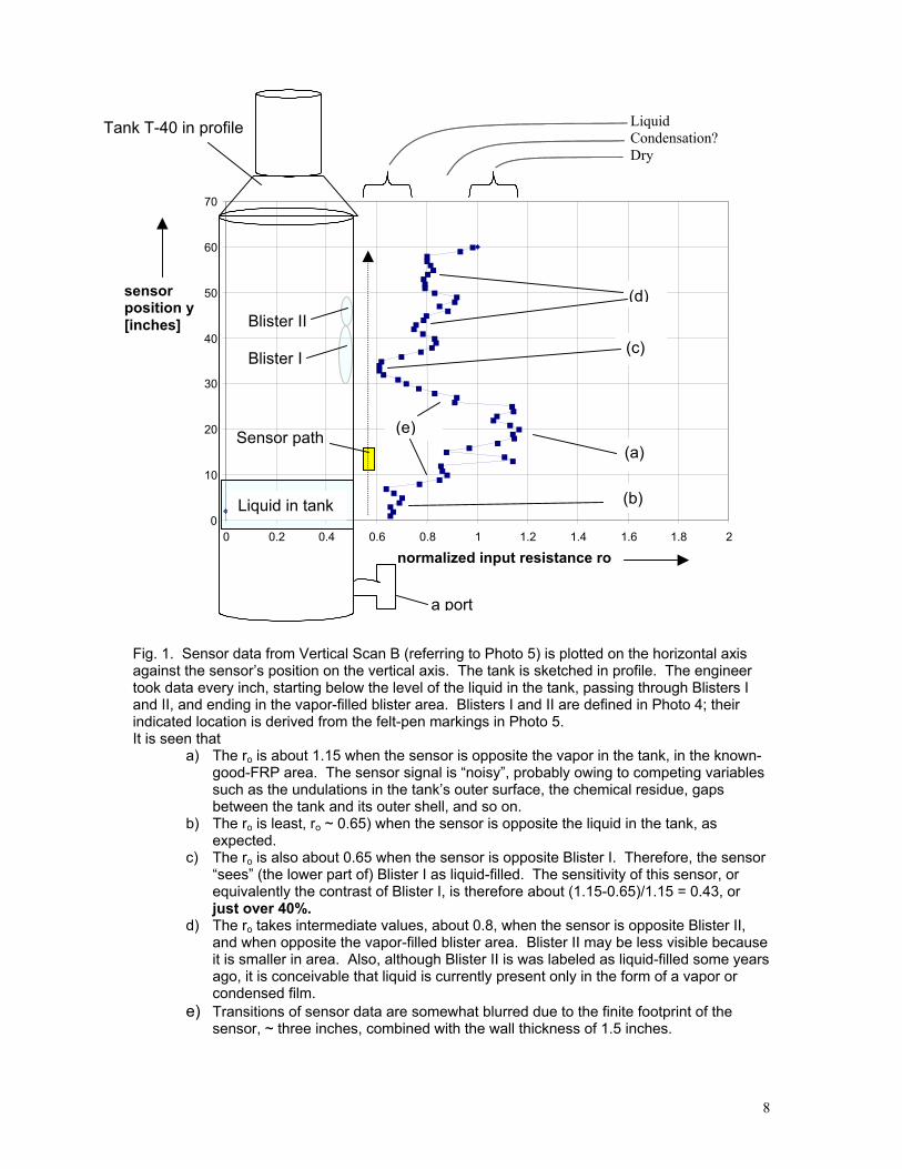
Fig. 1. Sensor data from Vertical Scan B (referring to Photo 5) is plotted on the horizontal axis against the sensor’s position on the vertical axis. The tank is sketched in profile. The engineer took data every inch, starting below the level of the liquid in the tank, passing through Blisters I and II, and ending in the vapor-filled blister area. Blisters I and II are defined in Photo 4; their indicated location is derived from the felt-pen markings in Photo 5. It is seen that

a) The ro is about 1.15 when the sensor is opposite the vapor in the tank, in the known-good-FRP area. The sensor signal is “noisy”, probably owing to competing variables such as the undulations in the tank’s outer surface, the chemical residue, gaps between the tank and its outer shell, and so on.

b) The ro is least, ro ~ 0.65) when the sensor is opposite the liquid in the tank, as expected.

c) The ro is also about 0.65 when the sensor is opposite Blister I. Therefore, the sensor “sees” (the lower part of) Blister I as liquid-filled. The sensitivity of this sensor, or equivalently the contrast of Blister I, is therefore about (1.15-0.65)/1.15 = 0.43, or just over 40%.

d) The ro takes intermediate values, about 0.8, when the sensor is opposite Blister II, and when opposite the vapor-filled blister area. Blister II may be less visible because it is smaller in area. Also, although Blister II is was labeled as liquid-filled some years ago, it is conceivable that liquid is currently present only in the form of a vapor or condensed film.

e) Transitions of sensor data are somewhat blurred due to the finite footprint of the sensor, ~ three inches, combined with the wall thickness of 1.5 inches.

8

0

10

20

30

40

50

60

70

0 0.2 0.4 0.6 0.8 1 1.2 1.4

normalized input resistance ro

sens

or p

ositi

on y

[inc

hes]

Blister III and its data

(a) & (b)

The port, c.f. Fig. 1

Blisters I and II and their data

III

I

T-40, face on

II

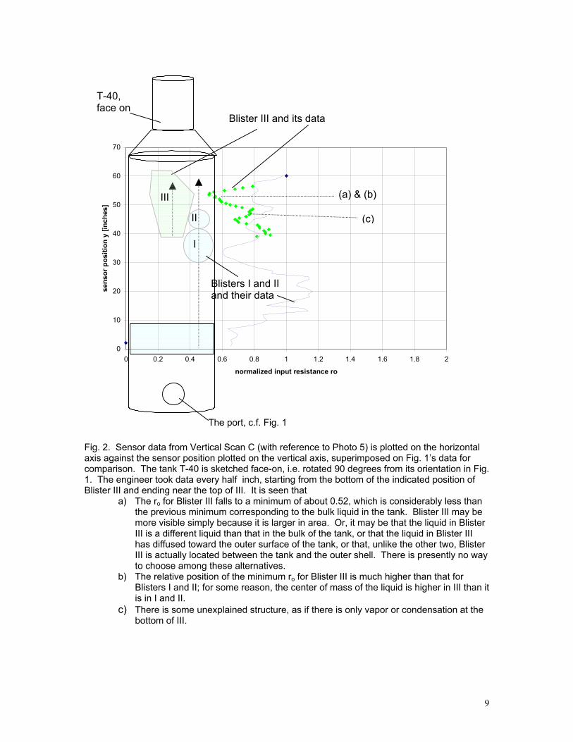
Fig. 2. Sensor data from Vertical Scan C (with reference to Photoaxis against the sensor position plotted on the vertical axis, supericomparison. The tank T-40 is sketched face-on, i.e. rotated 90 de1. The engineer took data every half inch, starting from the bottomBlister III and ending near the top of III. It is seen that

a) The ro for Blister III falls to a minimum of about 0.52, wthe previous minimum corresponding to the bulk liquidmore visible simply because it is larger in area. Or, it III is a different liquid than that in the bulk of the tank, has diffused toward the outer surface of the tank, or thIII is actually located between the tank and the outer sto choose among these alternatives.

b) The relative position of the minimum ro for Blister III isBlisters I and II; for some reason, the center of mass ois in I and II.

c) There is some unexplained structure, as if there is onlbottom of III.

(c)

1.6 1.8 2

5) is plotted on the horizontal mposed on Fig. 1’s data for grees from its orientation in Fig.

of the indicated position of

hich is considerably less than in the tank. Blister III may be may be that the liquid in Blister or that the liquid in Blister III at, unlike the other two, Blister hell. There is presently no way

much higher than that for f the liquid is higher in III than it

y vapor or condensation at the

9

IV

I

II

III

0

0.1

0.2

0.3

0.4

0.5

0.6

0.7

0.8

0.9

1

0 5 10 15 20 25 30 35

distance [inches]

inpu

t res

ista

nce

ro I

II

III

IV

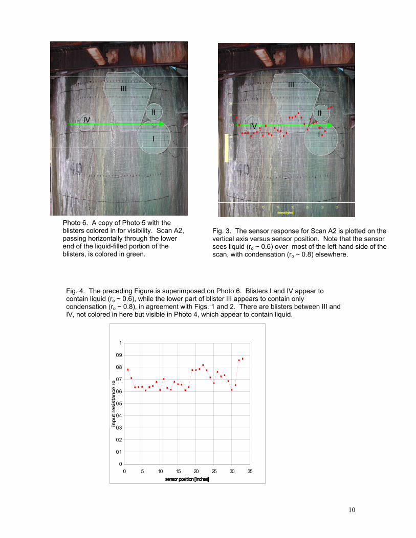
Photo 6. A copy of Photo 5 with the blisters colored in for visibility. Scan A2, passing horizontally through the lower end of the liquid-filled portion of the blisters, is colored in green.

Fig. 3. The sensor response for Scan A2 is plotted on the vertical axis versus sensor position. Note that the sensor sees liquid (ro ~ 0.6) over most of the left hand side of the scan, with condensation (ro ~ 0.8) elsewhere.

Fig. 4. The preceding Figure is superimposed on Photo 6. Blisters I and IV appear to contain liquid (ro ~ 0.6), while the lower part of blister III appears to contain only condensation (ro ~ 0.8), in agreement with Figs. 1 and 2. There are blisters between III and IV, not colored in here but visible in Photo 4, which appear to contain liquid.

0

0.1

0.2

0.3

0.4

0.5

0.6

0.7

0.8

0.9

1

0 5 10 15 20 25 30 35sensor position [inches]

inpu

t res

ista

nce

ro

10

IV

I

II

III

0

0.2

0.4

0.6

0.8

1

1.2

0 5 10 15 20 25 30 35

inpu

t res

ista

nce

ro

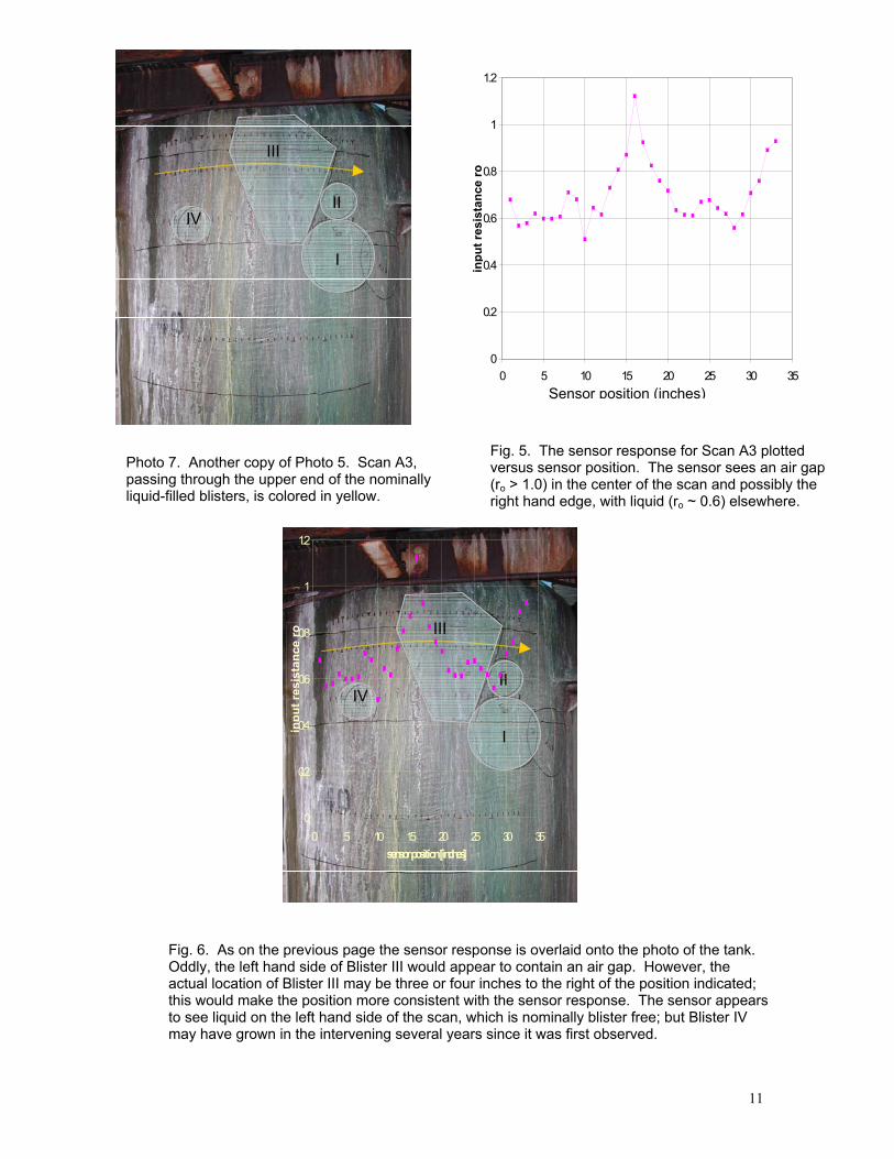
Fig. 5. Tversus s(ro > 1.0right han

Photo 7. Another copy of Photo 5. Scan A3, passing through the upper end of the nominally liquid-filled blisters, is colored in yellow.

III

II

I

IV

0

0.2

0.4

0.6

0.8

1

1.2

0 5 10 15 20 25 30 35sensor position [inches]

inpu

tres

ista

nce

ro

Fig. 6. As on the previous page the sensor response is ovOddly, the left hand side of Blister III would appear to contactual location of Blister III may be three or four inches to this would make the position more consistent with the sento see liquid on the left hand side of the scan, which is nommay have grown in the intervening several years since it w

Sensor position (inches)

he sensor response for Scan A3 plotted ensor position. The sensor sees an air gap ) in the center of the scan and possibly the d edge, with liquid (ro ~ 0.6) elsewhere.

erlaid onto the photo of the tank. ain an air gap. However, the the right of the position indicated; sor response. The sensor appears

inally blister free; but Blister IV as first observed.

11

IV II

I

0

0.2

0.4

0.6

0.8

1

1.2

1.4

0 5 10 15 20 25 30 35sensor position [inches]

inpu

t res

ista

nce

ro

III

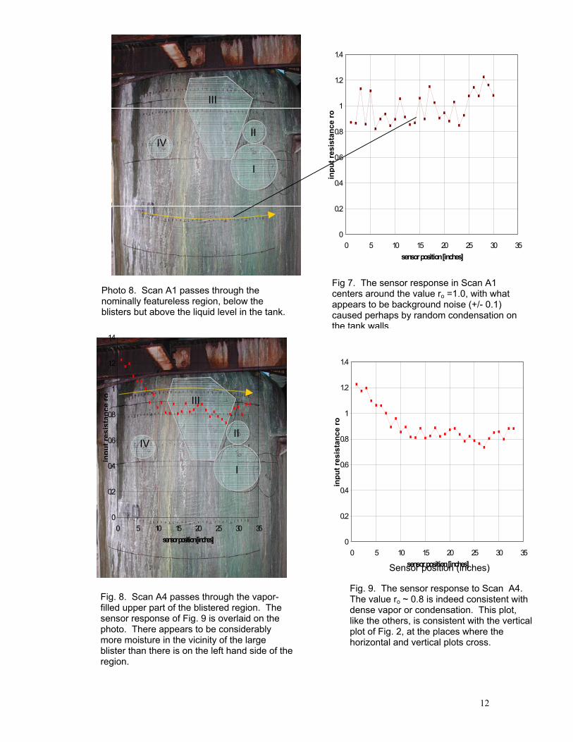
Photo 8. Scan A1 passes through the

nominally featureless region, below the blisters but above the liquid level in the tank.

III

II

I

IV

00 5

0.2

0.4

0.6

0.8

1

1.2

1.4

10 15 20 25 30 35sensor position [inches]

inpu

tres

ista

nce

ro

Fig. 8. Scan A4 passes through the vapor-filled upper part of the blistered region. The sensor response of Fig. 9 is overlaid on the photo. There appears to be considerably more moisture in the vicinity of the large blister than there is on the left hand side of the region.

Fig 7. The sensor response in Scan A1 centers around the value ro =1.0, with what appears to be background noise (+/- 0.1) caused perhaps by random condensation on the tank walls.

0

0.2

0.4

0.6

0.8

1

1.2

1.4

0 5 10 15 20 25 30 35

inpu

t res

ista

nce

ro

sensor position [inches]Sensor position (inches)

Fig. 9. The sensor response to Scan A4. The value ro ~ 0.8 is indeed consistent with dense vapor or condensation. This plot, like the others, is consistent with the vertical plot of Fig. 2, at the places where the horizontal and vertical plots cross.

12

13

ANALYSIS AND RECOMMENDATIONS The data from the two sets of scans appear to be self-consistent and to correspond with what is known of the physical reality, on the whole. The contrast between blistered and known-good areas is striking, despite the huge wall thickness and other competing variables that contribute to variability in some of the data. It is encouraging that the tank could be tested while it was in service. The data appears to be repeatable because the horizontal scans agree numerically with the vertical scans where they cross, and because the liquid in the bottom of the tank gives about the same ro as the liquid in the blisters. The discrepancy between expected and actual sensor data on the left side of Fig. 5 requires interpretation. It seems plausible to invoke the difficulty of transferring the photo records from the interior to the exterior of the tank. Growth of the blisters may also play a role. The difference between the liquid mass distribution between the two blisters in Fig. 2 is rather odd. There is a lot more liquid in the upper part of the largest blister, whereas the smallish blister off to the right has most of its liquid on the bottom, if the sensor data is to be believed. It appears that the sensor is able to identify features that are not apparent even from photos of the tank interior, although the nature of these features is still uncertain. Ultimately tests should be done on a single tank with a wide range of blister sizes, from the very large to the very small, in order to gain insight into and to quantify the threshold of visibility of the blister, for a given wall thickness and given liquid filling. Sensor design would benefit enormously from the existence of such a tank. Although each plant visit is a learning experience, it is difficult to think of a consistent way to amalgamate all the data taken piecemeal from separate plant visits. If the sensor continues to provide useful data, it would be enlightening to work with a blister expert, to gain insight into whether the threshold of blister visibility is lower than some threshold of tolerable hazard. Incidentally, the Akzo plant may have a third tank available, to be discarded some time in 2002. This tank may very well have such a range of blister sizes; and, for the first time we are enticed by the prospect of putting the whole effort on a scientific basis by correlating destructive testing with NDT, if the tank can be retrieved with liquid filled blisters intact. This tank is about three feet in diameter and four to five feet tall. Submitted by Michael Werner, Ph.D. KDC Technology Corp 2011 Research Dr. Livermore CA 94550 (925) 449-4770 kdc@ant-s.com