NONDESTRUCTIVE EVALUATION

OF ADHESIVE BONDS

A thesis submitted in partial fulfillment of the requirement

for the degree of Bachelor of Sciences with Honors in

Physics from the College of William and Mary in Virginia,

by

Chandler Harris Amiss

Accepted for __________________________

(Honors, High Honors, or Highest Honors)

_____________________________________

_______________________________Director

_____________________________________

_____________________________________

_____________________________________

Williamsburg, Virginia

April 1999

2

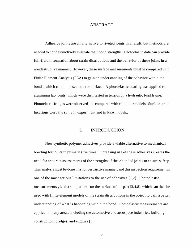
ABSTRACT

Adhesive joints are an alternative to riveted joints in aircraft, but methods are

needed to nondestructively evaluate their bond strengths. Photoelastic data can provide

full-field information about strain distributions and the behavior of these joints in a

nondestructive manner. However, these surface measurements must be compared with

Finite Element Analysis (FEA) to gain an understanding of the behavior within the

bonds, which cannot be seen on the surface. A photoelastic coating was applied to

aluminum lap joints, which were then tested in tension in a hydraulic load frame.

Photoelastic fringes were observed and compared with computer models. Surface strain

locations were the same in experiment and in FEA models.

I. INTRODUCTION

New synthetic polymer adhesives provide a viable alternative to mechanical

bonding for joints in primary structures. Increasing use of these adhesives creates the

need for accurate assessments of the strengths of these bonded joints to ensure safety.

This analysis must be done in a nondestructive manner, and this inspection requirement is

one of the most serious limitations to the use of adhesives [1,2]. Photoelastic

measurements yield strain patterns on the surface of the part [3,4,8], which can then be

used with finite element models of the strain distributions in the object to gain a better

understanding of what is happening within the bond. Photoelastic measurements are

applied in many areas, including the automotive and aerospace industries, building

construction, bridges, and engines [3].

3

II. MOTIVATION

Manufacturers would like to use adhesives rather than rivets or welds in structural

applications. Adhesives used in structural applications have the inherent advantage of

joining similar or dissimilar materials without changing the microstructure of the

adherents (substrates) as would occur with welding. They also provide a larger load-

bearing area than do mechanical fasteners, thereby distributing stresses more uniformly

and reducing stress concentrations, compared to rivets or other mechanical fasteners. In

addition, not only simple, but also complex shapes can be joined. Galvanic and

electrochemical corrosion between dissimilar materials can also be prevented, and

altering the properties of the adhesive can control heat transfer and electrical

conductivity. Additionally, adhesive bonds can provide environmental sealing and

vibration damping. Most importantly, adhesive joints can provide favorable strength-to-

weight ratios and are frequently faster and cheaper to produce than mechanical joints, and

they are also more reliable [1,2,5].

A nondestructive technique is needed to evaluate the strength of adhesive bonds

for in-service joints. Photoelasticity is an optical technique that uses a special strain-

sensitive coating on the test object that exhibits fringe patterns when illuminated with

polarized light. These patterns can be read like a topographic map to visualize the strain

distribution over the surface o f the test object. Photoelasticity measures the difference of

the principal strains and the principal strain directions. It is non-contact, nondestructive,

and allows the measurement of strain fields over large areas quickly using images which

can be digitally archived and enhanced. This is preferable to the use of strain gages that

4

only provide point information in comparison with the full-field information generated

with photoelastic measurements [3,4,8].

However, photoelasticity can provide only surface information and must be

combined with computer models to obtain information about strain distributions within a

bond. Models are generated because lap joints are too complicated in most cases to allow

an analytical solution of the continuum mechanics [2]. Once a model has been created,

the strains in the model can be compared with photoelastic measurements.

III. THEORY

1. Strength of Materials

Knowledge of the mechanics of materials is necessary to understand the finite

element models. Stress is a force per unit area. In the case of uniaxial stress with

uniform deformation,

AP

avg =σ (1)

and

AV

avg =τ (2)

where avgσ is the average normal stress, P is the normal force, A is the area over which

the force is applied, avgτ is the average shear stress (acting parallel to the face of the

object), and V is the shear force. Strain ( ε) is the fractional change in length of an object

(∆L/L) under stress. It is often related to the stress by Hooke’s law: εσ E= , where E is

5

Young’s modulus, also called the modulus of elasticity, or stiffness. Strain is much less

than unity for infinitesimal deformation. The relationship between stress and strain can

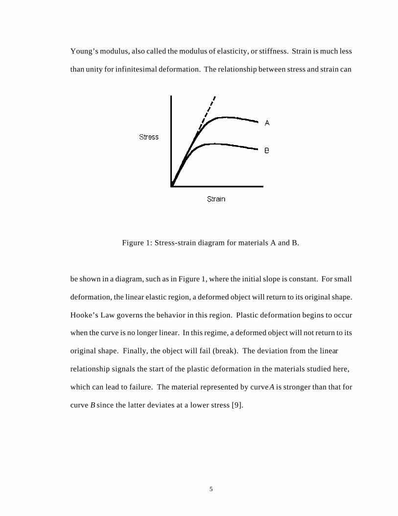
Figure 1: Stress-strain diagram for materials A and B.

be shown in a diagram, such as in Figure 1, where the initial slope is constant. For small

deformation, the linear elastic region, a deformed object will return to its original shape.

Hooke’s Law governs the behavior in this region. Plastic deformation begins to occur

when the curve is no longer linear. In this regime, a deformed object will not return to its

original shape. Finally, the object will fail (break). The deviation from the linear

relationship signals the start of the plastic deformation in the materials studied here,

which can lead to failure. The material represented by curve A is stronger than that for

curve B since the latter deviates at a lower stress [9].

6

2. Adhesive technology

The primary function of adhesives is to join materials or parts. The adhesive

transmits the stresses from one adherent to another such that the stresses are evenly

distributed. The adhesive fills the joint and creates bonding forces over the entire area,

rather than at discrete points, as with fasteners. Therefore, with lower and more uniform

stress levels and at a lower cost and weight, adhesives can provide structural load-

carrying capability greater than or equal to conventional fasteners. They can also be

faster to manufacture. The net result is lighter materials and structures [1,2].

Additional advantages of adhesives include the minimization or prevention of

electrochemical or galvanic corrosion between dissimilar materials. Environmental

sealing also increases corrosion resistance. Insulation against heat transfer or electrical

conductance is provided. Resistance to fatigue or cyclic loads, mechanical damping and

absorption of shock loads, and smooth joint contours are additional advantages. In most

cases, no reduction of adherent strength occurs because the curing heat of the adhesive is

usually below the heat needed to affect the adherent (e.g. metal or ceramic). Flexible

adhesives can join adherents with different thermal expansion coefficients without the

damage that might occur with stiff or rigid joints [1,2,6].

There are two types of adhesive bonding -- structural and nonstructural.

Structural adhesive bonds are defined by the strength of the adhesive. In this case, the

adhesive is strong enough that the structure can be stressed almost to the yield point of

the adherents. The full strength of the adherents can then be utilized, thus allowing high

joint efficiencies. In order to fulfill design criteria, the adhesive must be able to transmit

stresses, within the limits of the design, without losing its integrity. Generally, structural

7

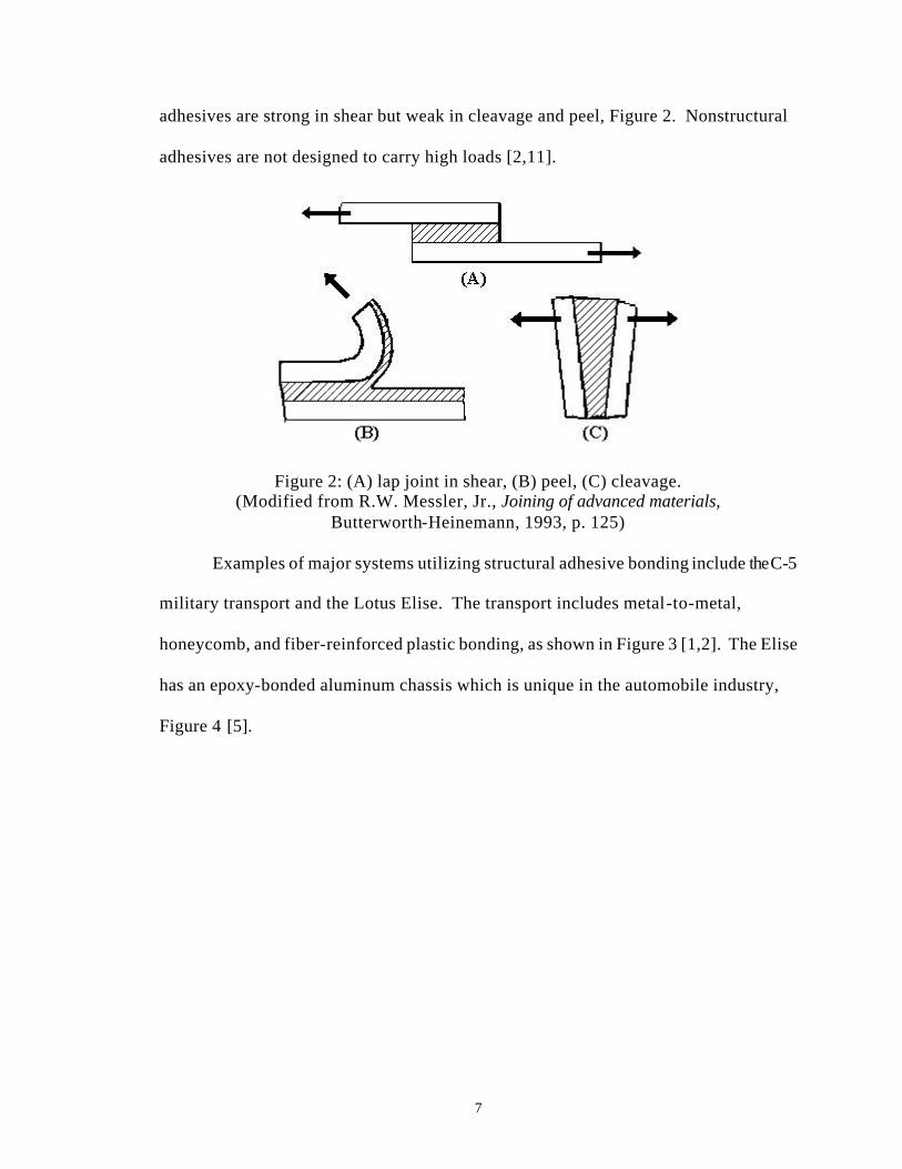
adhesives are strong in shear but weak in cleavage and peel, Figure 2. Nonstructural

adhesives are not designed to carry high loads [2,11].

Figure 2: (A) lap joint in shear, (B) peel, (C) cleavage. (Modified from R.W. Messler, Jr., Joining of advanced materials,

Butterworth-Heinemann, 1993, p. 125)

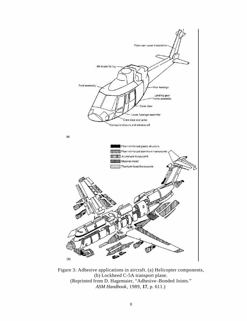
Examples of major systems utilizing structural adhesive bonding include the C-5

military transport and the Lotus Elise. The transport includes metal-to-metal,

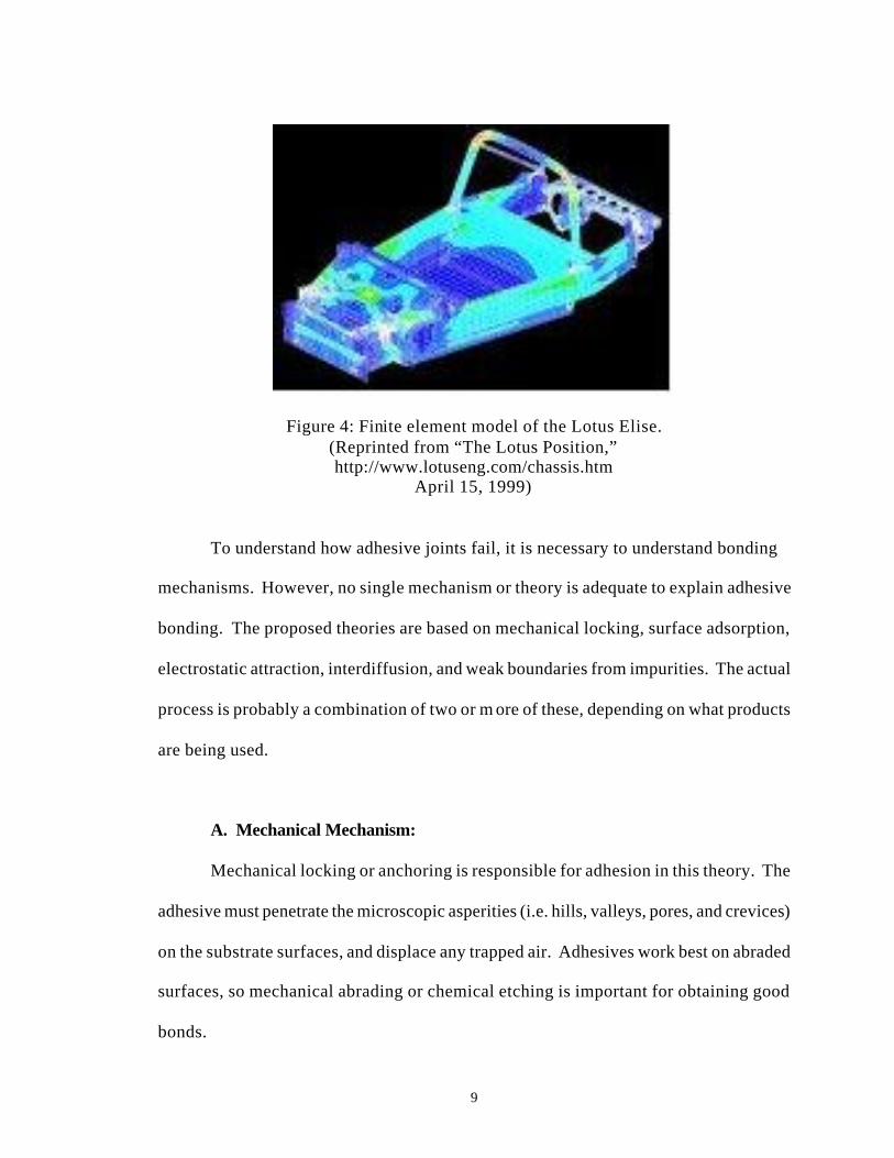
honeycomb, and fiber-reinforced plastic bonding, as shown in Figure 3 [1,2]. The Elise

has an epoxy-bonded aluminum chassis which is unique in the automobile industry,

Figure 4 [5].

8

Figure 3: Adhesive applications in aircraft. (a) Helicopter components, (b) Lockheed C-5A transport plane.

(Reprinted from D. Hagemaier, “Adhesive -Bonded Joints.” ASM Handbook, 1989, 17, p. 611.)

9

Figure 4: Finite element model of the Lotus Elise. (Reprinted from “The Lotus Position,” http://www.lotuseng.com/chassis.htm

April 15, 1999)

To understand how adhesive joints fail, it is necessary to understand bonding

mechanisms. However, no single mechanism or theory is adequate to explain adhesive

bonding. The proposed theories are based on mechanical locking, surface adsorption,

electrostatic attraction, interdiffusion, and weak boundaries from impurities. The actual

process is probably a combination of two or m ore of these, depending on what products

are being used.

A. Mechanical Mechanism:

Mechanical locking or anchoring is responsible for adhesion in this theory. The

adhesive must penetrate the microscopic asperities (i.e. hills, valleys, pores, and crevices)

on the substrate surfaces, and displace any trapped air. Adhesives work best on abraded

surfaces, so mechanical abrading or chemical etching is important for obtaining good

bonds.

10

Several factors may contribute to the effect of abrasion, including enhanced

mechanical interlocking, creating a clean surface, forming a highly chemically reactive

surface, and increasing the bonding surface area by roughing the surface. A combination

of the increased surface area and chemical reactivity work together to produce the

stronger bond. Mechanical bonding is likely involved in most bonds, alone or in

combination with other mechanisms of adhesion [2].

B. Adsorption Mechanism:

In this theory, molecular contact between adhesive and adherent, with the

resulting surface forces that develop, is responsible for the adhesive force. Wetting is the

process that establishes intimate contact between the adhesive and adherent. A liquid

“spontaneously” adheres to and spreads on a solid surface. It is controlled by the surface

energy of the liquid-solid interface versus the liquid-vapor and solid-vapor interfaces.

The surface is completely wet if the angle of contact (θ) between the surface and the

liquid is zero. Incomplete wetting occurs at any other angle. Any contact angle less than

90 degrees indicates reasonable wetting for bonding. For proper wetting, the surface

tension of the adhesive should be lower than that of the adherent. Good wetting occurs

when the adhesive fills the microscopic hills and valleys on the surface of the adherent

while in poor wetting, the adhesive bridges the valleys. The resulting decrease in the

actual contact area lowers the joint strength [2,11].

After wetting, chemical bonding is theorized to be responsible for the bond

strength. The chemical bonds in adhesion or cohesion can be primary (e.g. ionic,

covalent, or metallic bonds), but are usually secondary (e.g. Van der Waals attractions or

11

permanent dipole moments). Adhesion occurs when different materials are held together

by physical and/or chemical valence forces such that work is necessary to separate them.

Cohesion occurs when primary or secondary chemical valences hold together particles of

a single substance. The type of bonding that predominates depends on the material, but

secondary bonding is theorized to contribute to all bonding [2].

C. Electrostatic Theory:

In this theory, adhesion is due to electrostatic forces between the adhesive and

adherent at their interface. A layer of separated charge at the interface holds the adhesive

and adherent together. Electrical discharges have been seen when materials were

separated, supporting this theory. Permanent dipoles or polar molecules most likely

account for this type of bonding [2].

D. Diffusion Mechanism:

The interdiffusion of molecules is primarily responsible for adhesion in the

diffusion theory. The chances of diffusion occurring increase with similar adhesive and

adherent, such as when both are polymers. The long chains may be mobile enough to

diffuse and entangle. Entanglement is important in joining polymers, especially

thermoplastics. This theory is not as applicable to the adhesive bonding of metals or

ceramics, and secondary bonding does not play a role here [2].

12

E. Weak-Boundary Layer Theory:

Weak-boundary layer theory explains the failure of joints more than their

adhesion. Most bonds fail just next to the interface, suggesting a weak boundary layer

adjacent to the interface. This could result from a chemical reaction between adhesive

and adherent. Contamination of, or impurity concentrations in, the surface layer could

also be responsible. Sources of weak boundary layers are (1) concentrations of low

molecular weight compounds from separation of adhesive components during bonding,

(2) oxides, sulfides, and other chemical layers on metals which are weakly bound, and (3)

air trapped at the interface.

Bond failures can provide information about the mechanisms by which bonds fail.

The dominant types of failure are adhesive and cohesive failure. Adhesive failure is the

interfacial failure between adhesive and adherent. It is indicative of a weak-boundary

layer, often from improper preparation. In cohesive failure, a fracture occurs and

adhesive remains on both adherent surfaces. When the adherent fails before the adhesive,

the fracture is contained completely within the adherent. This is known as the cohesive

failure of the substrate. Optimal failure is cohesive, because the maximum strength of the

materials in the joint has been reached, and no questions arise about improper preparation

or bonding.

Causes of premature failure are very difficult to determine, especially in bonded

joints. Failure could come from incomplete wetting, internal stresses arising from

adhesive shrinkage during setting, or from different coefficients of thermal expansion.

Also important are the stresses, their orientation to the bond, and the rate of stress

13

application. Operating environmental factors can also have significant and synergistic

adverse effects. Currently, the best way of determining joint strength is by simulating a

joint in its operating conditions [2].

Many different types of flaws or discontinuities can occur in adhesive bonds.

Metal-to-metal voids are the most common flaws. Interface defects result from errors in

the preparation of the adherents. These can be reduced by careful process control,

adherence to specification requirements, and inspection procedures before continuing in

the bonding process. Disbonds can be found with current nondestructive techniques, but

they cannot easily determine joint strength [1].

F. Surface preparation

The objective of adhesive bonding is a bond providing maximum strength and

quality for a combination of adhesive and adherent, usually at minimum cost. Some

requirements which must be met include the cleanliness of the adherent surfaces prior to

bonding, proper wetting, adhesive choice, and joint design.

Since bonding is a surface phenomenon, joint cleanliness is essential. Any

foreign material must be removed. This includes dirt, grease, cutting coolants and

lubricants, water, and weak surface scales (e.g. oxides, sulfides). If they are not removed,

the adhesive can not adhere and the joint strength is compromised.

Surface preparation (or pretreatment) usually involves the following steps: solvent

cleaning, intermediate chemical and mechanical cleaning, and chemical treatment.

Solvent cleaning is always performed, and the other steps are performed as necessary,

14

though always in the same order. Priming may be done last, particularly under severe

environmental conditions [2,3,4,6,10,11].

3. Photoelasticity

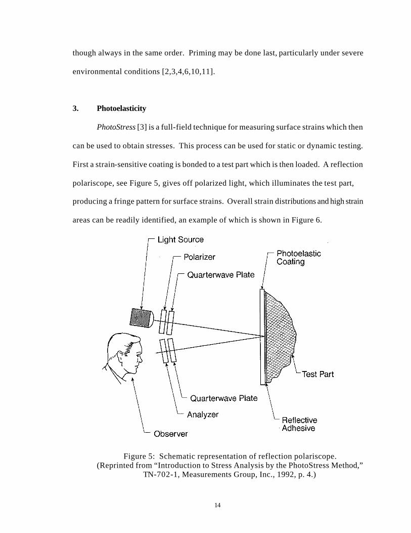
PhotoStress [3] is a full-field technique for measuring surface strains which then

can be used to obtain stresses. This process can be used for static or dynamic testing.

First a strain-sensitive coating is bonded to a test part which is then loaded. A reflection

polariscope, see Figure 5, gives off polarized light, which illuminates the test part,

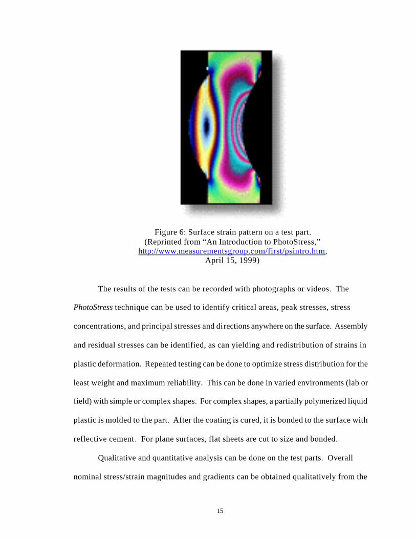
producing a fringe pattern for surface strains. Overall strain distributions and high strain

areas can be readily identified, an example of which is shown in Figure 6.

Figure 5: Schematic representation of reflection polariscope. (Reprinted from “Introduction to Stress Analysis by the PhotoStress Method,”

TN-702-1, Measurements Group, Inc., 1992, p. 4.)

15

Figure 6: Surface strain pattern on a test part. (Reprinted from “An Introduction to PhotoStress,”

http://www.measurementsgroup.com/first/psintro.htm, April 15, 1999)

The results of the tests can be recorded with photographs or videos. The

PhotoStress technique can be used to identify critical areas, peak stresses, stress

concentrations, and principal stresses and directions anywhere on the surface. Assembly

and residual stresses can be identified, as can yielding and redistribution of strains in

plastic deformation. Repeated testing can be done to optimize stress distribution for the

least weight and maximum reliability. This can be done in varied environments (lab or

field) with simple or complex shapes. For complex shapes, a partially polymerized liquid

plastic is molded to the part. After the coating is cured, it is bonded to the surface with

reflective cement. For plane surfaces, flat sheets are cut to size and bonded.

Qualitative and quantitative analysis can be done on the test parts. Overall

nominal stress/strain magnitudes and gradients can be obtained qualitatively from the

16

full-field fringe patterns. Quantitative measurements include the directions of principal

stresses and strains everywhere, as well as the magnitudes and signs of tangential stresses

along free (unloaded) boundaries and where the stress is uniaxial. In a biaxial stress

state, the magnitude and sign of the difference in principal stresses and strains can be

obtained at any point on the surface.

Full-field observation of strain distributions allows visual identification of

overstressed areas. Fringe orders are designated by color, where there is a relationship

between fringe order and strain magnitude. Loads cause stresses throughout the material

and on the surface. Intimate contact of the coating and test part allows the transmission

of strains within the material to the coating. The strains in the coating produce

isochromatic fringes when viewed with a reflection polariscope which are proportional to

the strains at the surface [3,4].

A. Theory of Photoelasticity

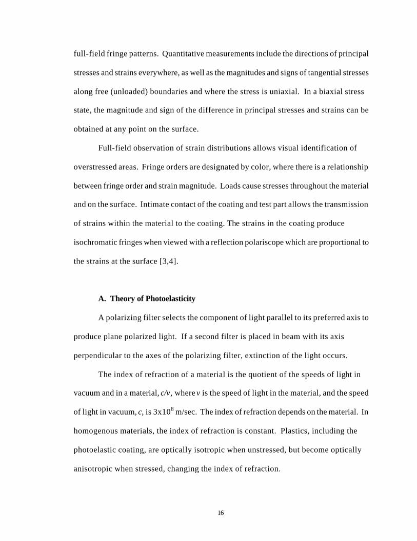
A polarizing filter selects the component of light parallel to its preferred axis to

produce plane polarized light. If a second filter is placed in beam with its axis

perpendicular to the axes of the polarizing filter, extinction of the light occurs.

The index of refraction of a material is the quotient of the speeds of light in

vacuum and in a material, c/v, where v is the speed of light in the material, and the speed

of light in vacuum, c, is 3x108 m/sec. The index of refraction depends on the material. In

homogenous materials, the index of refraction is constant. Plastics, including the

photoelastic coating, are optically isotropic when unstressed, but become optically

anisotropic when stressed, changing the index of refraction.

17

Figure 7. Schematic representation of the polarization of light. (Reprinted from “Introduction to Stress Analysis by the PhotoStress Method,”

TN-702-1, Measurements Group, Inc., 1992, p. 2.)

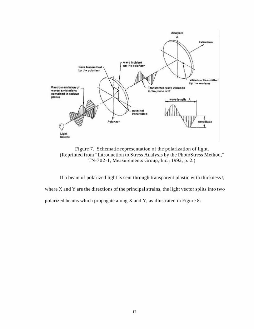
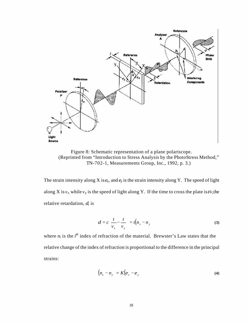
If a beam of polarized light is sent through transparent plastic with thickness t,

where X and Y are the directions of the principal strains, the light vector splits into two

polarized beams which propagate along X and Y, as illustrated in Figure 8.

18

Figure 8: Schematic representation of a plane polariscope. (Reprinted from “Introduction to Stress Analysis by the PhotoStress Method,”

TN-702-1, Measurements Group, Inc., 1992, p. 3.)

The strain intensity along X is εx, and εy is the strain intensity along Y. The speed of light

along X is vx while vy is the speed of light along Y. If the time to cross the plate is t/v, the

relative retardation, δ, is

( )yxyx

nntvt

vt

c −=

−=δ (3)

where ni is the ith index of refraction of the material. Brewster’s Law states that the

relative change of the index of refraction is proportional to the difference in the principal

strains:

( ) ( )yxyx Knn εε −=− (4)

19

K is the strain-optical coefficient, which is a dimensionless constant depending on the

material. Combining equations (1) and (2) yields:

( )yxtK εεδ −= (5)

for transmission, and

( )yxtK εεδ −= 2 (6)

for reflection. The factor of two appears since the light passes through the coating twice.

The equation for strain measurement in the photoelastic coating is:

(7)

The waves propagating along the X and Y directions are no longer in phase due to the

applied strain causing a relative retardation, δ. The separated waves are called the

ordinary and extraordinary. δ is the phase difference after the ordinary and extraordinary

waves pass through the analyzer filter. For a plane polariscope, as in Figure 8, the

intensity is a function of retardation and the angle between the analyzer and the direction

of the principal strains (β-α):

(8)

The angle of the polarizer’s transmission axes is α with respect to the vertical, and β is

the angle of the principal strain axes with respect to the vertical. The intensity is zero

when (β-α)=0, or when the crossed polarizer/analyzer is parallel to direction of principal

strains. The plane polariscope is used to obtain the principal strain directions.

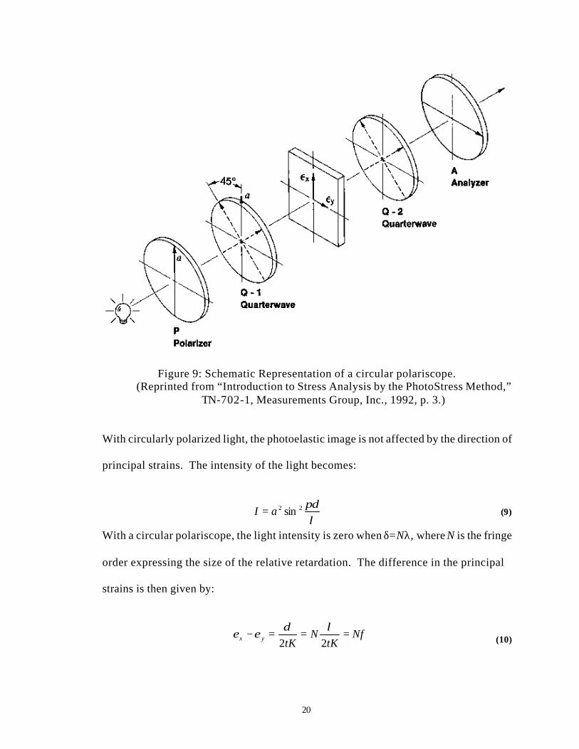
Circularly polarized light is obtained by adding quarter-wave plates (optical

filters) in the path of propagation of the linearly polarized light, as in Figure 9.

( )tKyx 2

δεε =−

λπδαβ 222 sin)(2sin −= aI

20

Figure 9: Schematic Representation of a circular polariscope. (Reprinted from “Introduction to Stress Analysis by the PhotoStress Method,”

TN-702-1, Measurements Group, Inc., 1992, p. 3.)

With circularly polarized light, the photoelastic image is not affected by the direction of

principal strains. The intensity of the light becomes:

(9)

With a circular polariscope, the light intensity is zero when δ=Nλ, where N is the fringe

order expressing the size of the relative retardation. The difference in the principal

strains is then given by:

(10)

λπδ22 sinaI =

NftK

NtKyx ===−

22

λδεε

21

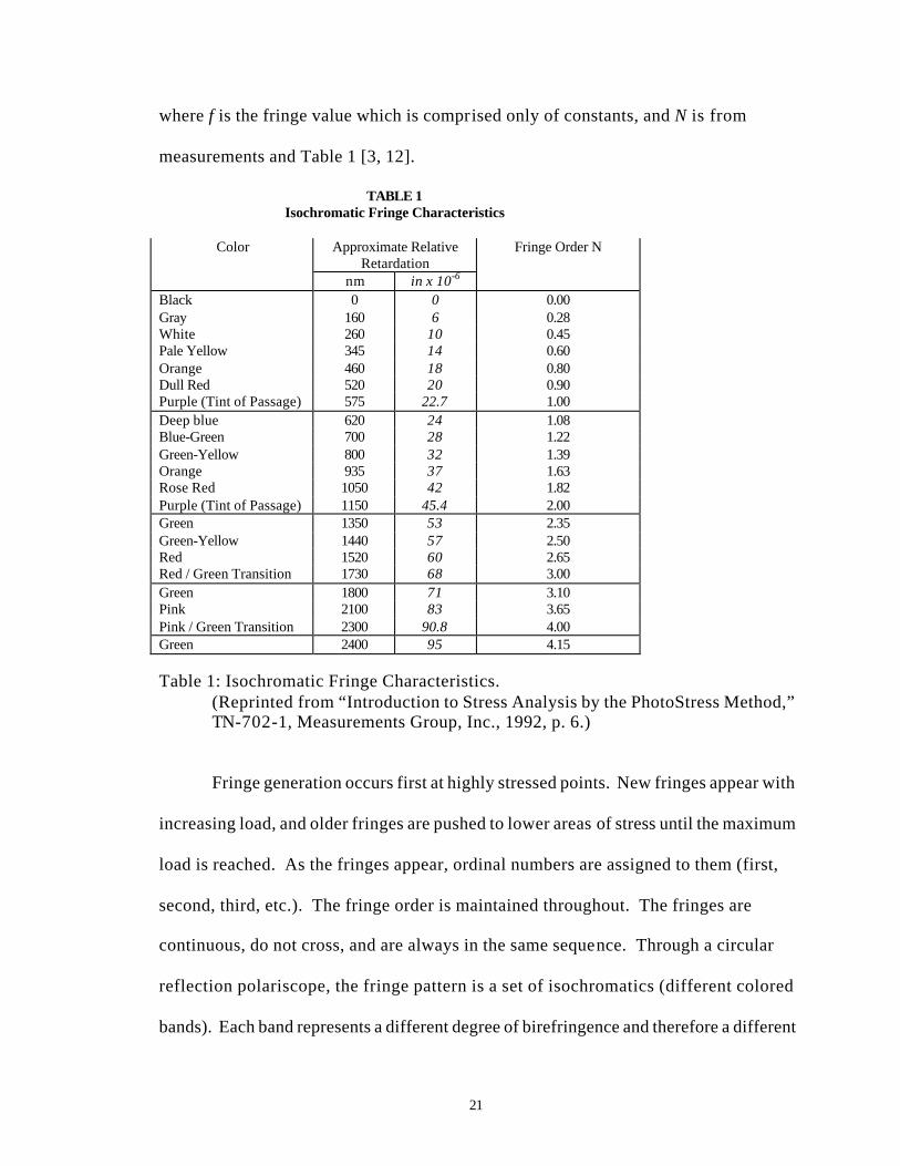
where f is the fringe value which is comprised only of constants, and N is from

measurements and Table 1 [3, 12].

TABLE 1 Isochromatic Fringe Characteristics

Approximate Relative

Retardation Color

nm in x 10-6

Fringe Order N

Black 0 0 0.00 Gray 160 6 0.28 White 260 10 0.45 Pale Yellow 345 14 0.60 Orange 460 18 0.80 Dull Red 520 20 0.90 Purple (Tint of Passage) 575 22.7 1.00 Deep blue 620 24 1.08 Blue-Green 700 28 1.22 Green-Yellow 800 32 1.39 Orange 935 37 1.63 Rose Red 1050 42 1.82 Purple (Tint of Passage) 1150 45.4 2.00 Green 1350 53 2.35 Green-Yellow 1440 57 2.50 Red 1520 60 2.65 Red / Green Transition 1730 68 3.00 Green 1800 71 3.10 Pink 2100 83 3.65 Pink / Green Transition 2300 90.8 4.00 Green 2400 95 4.15 Table 1: Isochromatic Fringe Characteristics.

(Reprinted from “Introduction to Stress Analysis by the PhotoStress Method,” TN-702-1, Measurements Group, Inc., 1992, p. 6.)

Fringe generation occurs first at highly stressed points. New fringes appear with

increasing load, and older fringes are pushed to lower areas of stress until the maximum

load is reached. As the fringes appear, ordinal numbers are assigned to them (first,

second, third, etc.). The fringe order is maintained throughout. The fringes are

continuous, do not cross, and are always in the same sequence. Through a circular

reflection polariscope, the fringe pattern is a set of isochromatics (different colored

bands). Each band represents a different degree of birefringence and therefore a different

22

level of strain. The fringe pattern can be read like a topological map when the fringe

order is understood.

As the light passes through the coating, the light rays undergo relative retardation.

The photoelastic effect is caused by constructive and destructive interference of these

phase shifted rays, which happens when the coating is stressed. With monochromatic

light, if the magnitude of the relative retardation is an integral multiple of the wavelength

(λ, 2λ, 3λ, etc.), cancellation and extinction occur, producing a black band. When the

relative retardation is an odd multiple of λ/2 ( λ/2, 3 λ/2, 5 λ/2, etc.), the rays are in phase

and add to maximum intensity. Intermediate magnitudes of the relative retardation give

intermediate intensities of light. The pattern appears as alternate light and dark f ringes

since the intensity is a sine-squared function of the relative retardation, see equations (8)

and (9).

White light, with all wavelengths of visible light, is most often used for the full-

field interpretation of the fringe patterns. When one wavelength of light is extinguished,

others are still visible. As each wavelength is extinguished with higher stresses, the

complementary color is seen. The complementary colors make up the fringe pattern for

white light. These colors are correlated with relative retardations and fringe orders in

Table 1 [3].

The photoelastic coating is viewed black when a coated, but unloaded, test part is

observed with a reflection polariscope. Colors appear as the part is loaded, with the

highest stressed areas getting color first. The colors appear in the following order: gray,

white, yellow (when violet is extinguished), orange (when blue goes), red

(complementary to green). Purple appears when yellow is extinguished, and then orange

23

is extinguished producing a blue fringe. The purple fringe is called the tint of passage. It

is easily distinguished from the red and blue on either side of it and is sensitive to small

changes in the strain. This fringe is used to designate the order of the fringes (N). As

tints of passage appear, the ordinal number increases (N=2, 3, etc.).

As the load is increased, the relative retardation increases and red is extinguished

(leaving blue-green for the fringe). Eventually the relative retardation is twice the

wavelength of purple, starting the fringe cycle again. However, the deep red at the far

end of the visible spectrum also has a wavelength twice that of violet and thus is

extinguished for the first time with the second violet extinction. This leaves a fringe that

is yellow and green, the complementary colors of red and violet. As a load is

progressively applied, the fringe colors cycle, but the colors are not the same as the first

order since multiple colors are extinguished simultaneously. Fringe colors become more

pale and less distinctive. Due to this effect, fringe orders above about 4 or 5 are not

distinguishable in white light, however fringe orders above 3 are rarely needed for the

stress analysis.

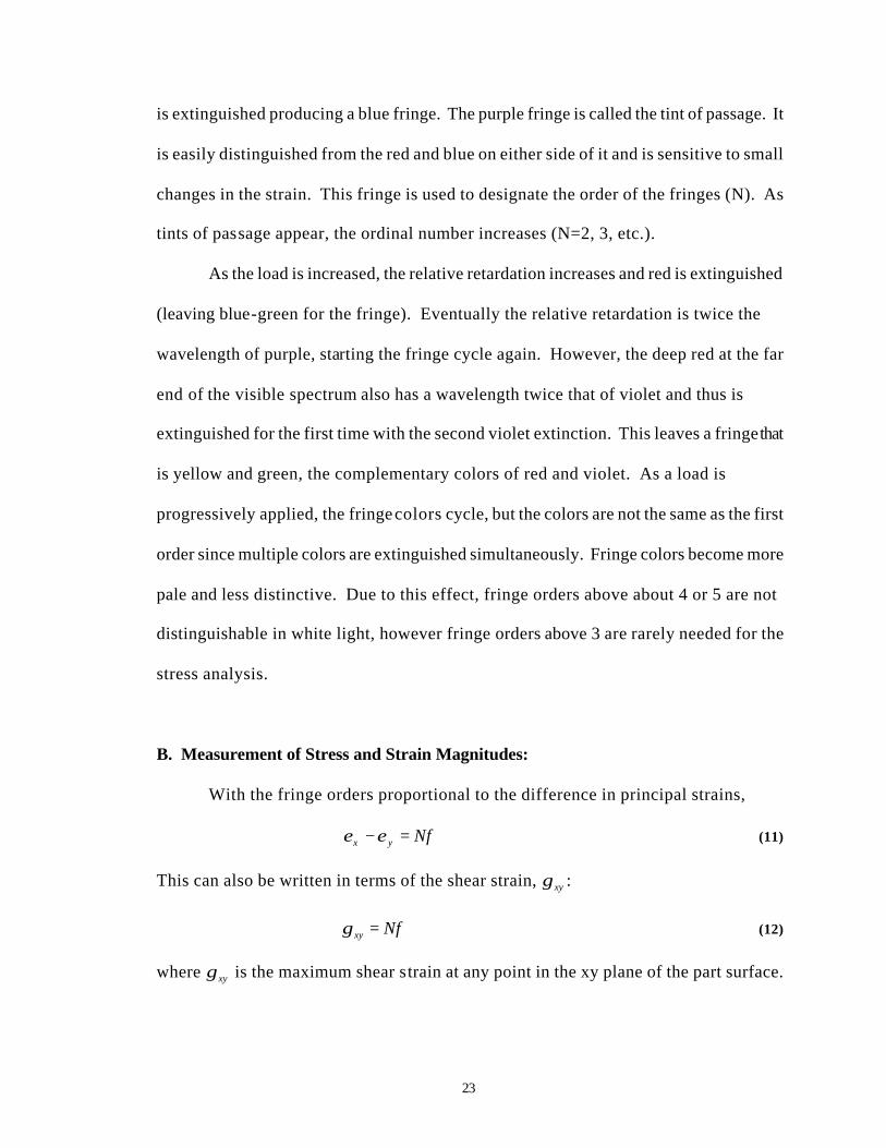
B. Measurement of Stress and Strain Magnitudes:

With the fringe orders proportional to the difference in principal strains,

Nfyx =−εε (11)

This can also be written in terms of the shear strain, xyγ :

Nfxy =γ (12)

where xyγ is the maximum shear strain at any point in the xy plane of the part surface.

24

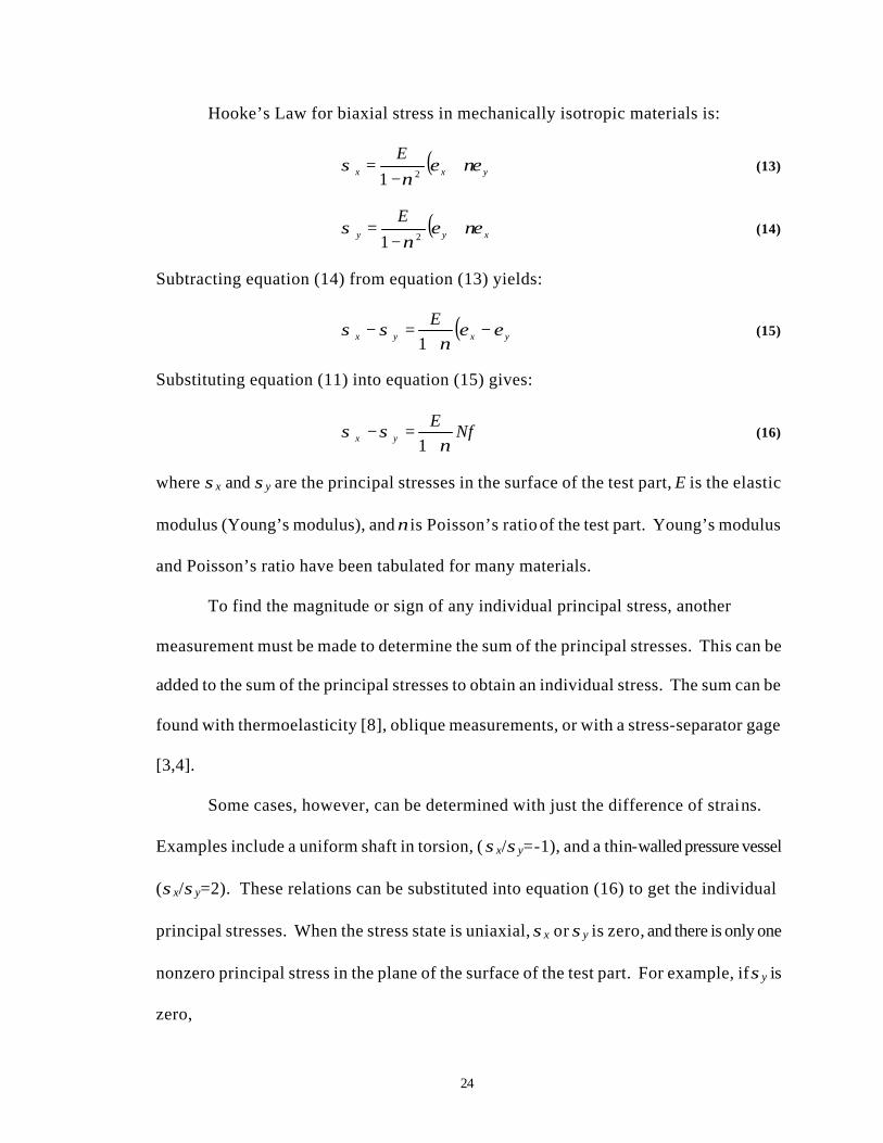
Hooke’s Law for biaxial stress in mechanically isotropic materials is:

( )yxx

Eνεε

νσ +

−=

21 (13)

( )xyy

Eνεε

νσ +

−=

21 (14)

Subtracting equation (14) from equation (13) yields:

( )yxyx

E εεν

σσ −+

=−1

(15)

Substituting equation (11) into equation (15) gives:

NfE

yx νσσ

+=−

1 (16)

where σx and σy are the principal stresses in the surface of the test part, E is the elastic

modulus (Young’s modulus), and ν is Poisson’s ratio of the test part. Young’s modulus

and Poisson’s ratio have been tabulated for many materials.

To find the magnitude or sign of any individual principal stress, another

measurement must be made to determine the sum of the principal stresses. This can be

added to the sum of the principal stresses to obtain an individual stress. The sum can be

found with thermoelasticity [8], oblique measurements, or with a stress-separator gage

[3,4].

Some cases, however, can be determined with just the difference of strains.

Examples include a uniform shaft in torsion, ( σx/σy=-1), and a thin-walled pressure vessel

(σx/σy=2). These relations can be substituted into equation (16) to get the individual

principal stresses. When the stress state is uniaxial, σx or σy is zero, and there is only one

nonzero principal stress in the plane of the surface of the test part. For example, if σy is

zero,

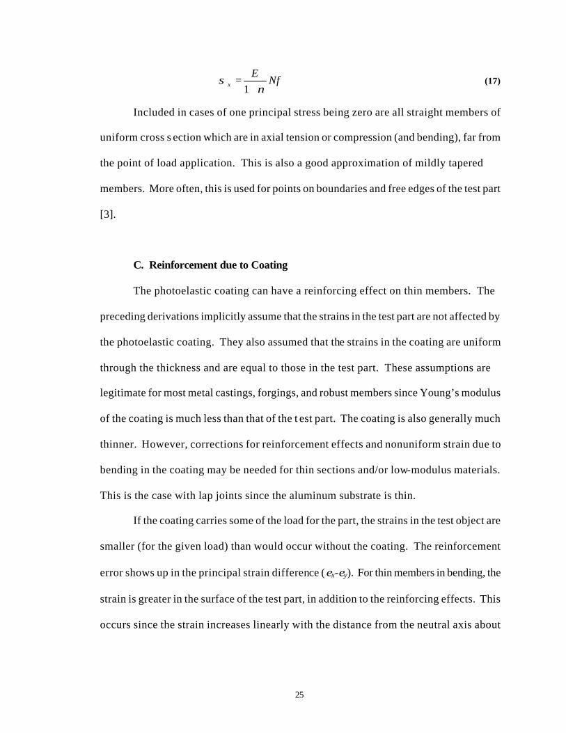
25

NfE

x νσ

+=

1 (17)

Included in cases of one principal stress being zero are all straight members of

uniform cross s ection which are in axial tension or compression (and bending), far from

the point of load application. This is also a good approximation of mildly tapered

members. More often, this is used for points on boundaries and free edges of the test part

[3].

C. Reinforcement due to Coating

The photoelastic coating can have a reinforcing effect on thin members. The

preceding derivations implicitly assume that the strains in the test part are not affected by

the photoelastic coating. They also assumed that the strains in the coating are uniform

through the thickness and are equal to those in the test part. These assumptions are

legitimate for most metal castings, forgings, and robust members since Young’s modulus

of the coating is much less than that of the t est part. The coating is also generally much

thinner. However, corrections for reinforcement effects and nonuniform strain due to

bending in the coating may be needed for thin sections and/or low-modulus materials.

This is the case with lap joints since the aluminum substrate is thin.

If the coating carries some of the load for the part, the strains in the test object are

smaller (for the given load) than would occur without the coating. The reinforcement

error shows up in the principal strain difference (εx-εy). For thin members in bending, the

strain is greater in the surface of the test part, in addition to the reinforcing effects. This

occurs since the strain increases linearly with the distance from the neutral axis about

26

which the bending occurs. Here the observed coating fringes correspond to the average

strain through the coating thickness (the strain at mid-thickness) [4].

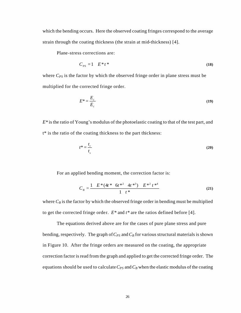
Plane-stress corrections are:

**1 tECPS += (18)

where CPS is the factor by which the observed fringe order in plane stress must be

multiplied for the corrected fringe order.

c

c

EE

E =* (19)

E* is the ratio of Young’s modulus of the photoelastic coating to that of the test part, and

t* is the ratio of the coating thickness to the part thickness:

s

c

tt

t =* (20)

For an applied bending moment, the correction factor is:

*1

**)*4*6*4(*1 4232

ttEtttE

CB +++++= (21)

where CB is the factor by which the observed fringe order in bending must be multiplied

to get the corrected fringe order. E* and t* are the ratios defined before [4].

The equations derived above are for the cases of pure plane stress and pure

bending, respectively. The graph of CPS and CB for various structural materials is shown

in Figure 10. After the fringe orders are measured on the coating, the appropriate

correction factor is read from the graph and applied to get the corrected fringe order. The

equations should be used to calculate CPS and CB when the elastic modulus of the coating

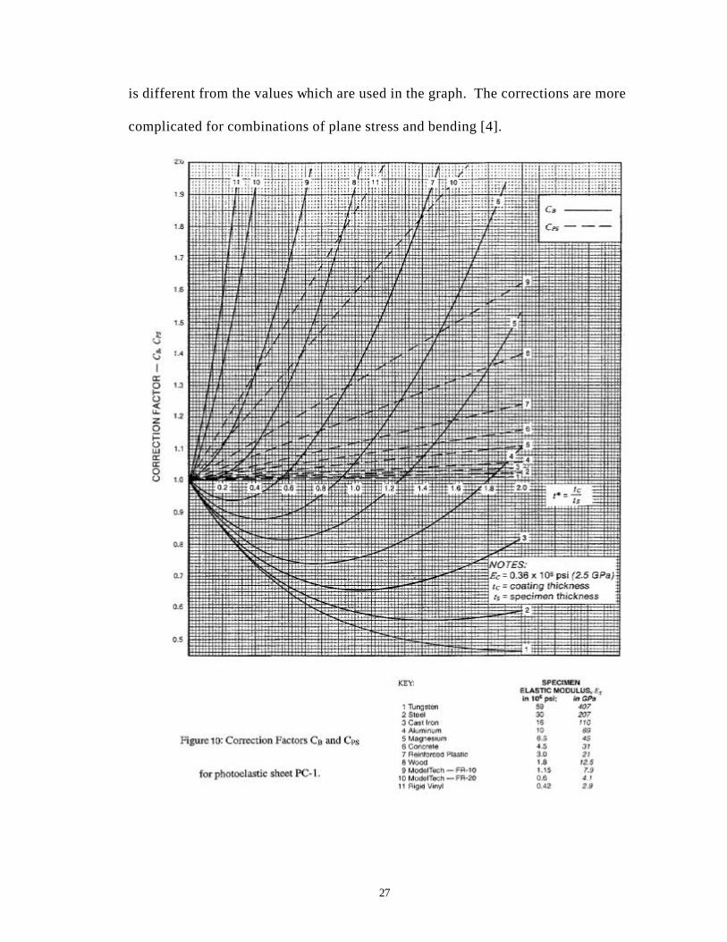
27

is different from the values which are used in the graph. The corrections are more

complicated for combinations of plane stress and bending [4].

28

4. Finite Element Analysis

A commercial finite element analysis package, COSMOS/M, was chosen

for its static structural capabilities to analyze the lap joints. Finite Element Analysis

(FEA) numerically approximates a continuous calculation by discretizing the problem

into elements, small units used for analysis. Each element is connected, directly or

indirectly, to all of the other elements through common interfaces (nodes, boundary lines,

and/or surfaces). Known material properties (including stress/strain relationships) are

then used to determine the behavior of any node in relation to the others. The resulting

equations are best expressed in matrix notation. For structural problems, usually the

displacements are calculated at each node and the stresses for each element subject to the

applied loads of the body. For example, in nonstructural problems, the nodal unknowns

may be temperatures due to thermal fluxes. The goal of FEA is to create a model as

detailed as possible, given a the resources of the computer.

Finite element analysis has many inherent advantages: it is easy to model irregular

shapes, and it is possible to evaluate different materials. FEA can apply general load

conditions, and large numbers and kinds of boundary conditions are possible. Different

sizes of elements can be used where necessary. The model can be altered relatively

cheaply and easily. Dynamic effects, nonlinear behaviors (from large displacements),

and nonlinear materials can be examined. Detection of problems from stress, vibrations,

and thermal effects can be addressed before construction of a prototype is begun. Finite

element analysis can also increase confidence in a prototype and reduce the number of

prototypes required in the design process [7,13,14].

Steps in the development of a finite element model follow:

29

Step 1: Discretize and choose element types.

Divide the continuous body into an equivalent set of finite elements and nodes.

This also involves choosing the most appropriate element type for the problem, which is

primarily a matter of engineering judgement. Elements should be small enough to give

useful information but large enough to reduce computational time and effort to a

manageable level. More elements should be used in areas of rapid change, while larger

(and fewer) elements should be used in areas of constancy. An example of an area of

rapid change would be a change in geometry. The choice of element type depends on the

makeup of the loaded body and how close the approximation needs to be. One-, two-,

and three-dimensional elements are available. This is one of the most important choices

the designer makes. For the lap joint, one inch corresponds to 32 units in the model, and

the model was scaled appropriately. The geometry of the lap joint was modeled with

volumes to form the correct shape.

The basic line elements are bar (or truss) and beam elements with cross-sectional

area, but usually represented by line segments. The area can vary. Line and beam

elements are often used to model trusses and frame structures. Linear elements are the

simplest with one node at each end. Quadratic, cubic, etc. elements also exist with three

or more nodes.

Two-dimensional (or plane) elements are loaded in their planes. They are

triangular or quadrilateral. The simplest are linear elements which have only corner

nodes and straight sides. Quadratic elements have midside nodes and can have curved

sides. Elements can have variable thicknesses or can be constant throughout. A wide

range of engineering problems can be modeled with these elements.

30

Tetrahedral and hexahedral (or brick) elements are the most common three-

dimensional elements, used when it is necessary to do a three-dimensional stress analysis.

Again, the basic elements have only corner nodes and straight sides, but higher-order

elements with midedge and midface nodes may have curved side surfaces. Tetrahedral

elements were chosen for the modeled lap joints [13].

Step 2: Choose a displacement function.

Choose a displacement function within each element using the nodal values of the

element. The most frequent equations are linear, quadratic, and cubic polynomials, but

trigonometric series can also be used. The function is used for each element and then

taken over the whole structure. The continuous nature of the structure is approximated

by a set of piecewise-continuous functions defined within each finite element (or domain)

[13].

Step 3: Define strain/displacement and stress/strain relationships.

These are necessary for each element. For example, a one-dimensional

deformation in the x direction will give for small strains (εx)

dxdu

x =ε (22)

where u is the displacement. Defining the material behavior accurately is essential for

good results. Hooke’s law is the simplest stress/strain law and is often used in analysis.

Criteria must be defined to determine where the linear relationship is no longer valid.

This is discussed in detail in reference [7].

31

Step 4: Derive the element stiffness matrix and equations.

The resulting equations are written in the following matrix form:

=

nnnn

n

n

n

n d

d

d

d

kk

kkkk

kkkk

kkkk

f

f

f

f

M

L

MOM

L

L

L

M3

2

1

1

3333231

2232221

1131211

3

2

1

(23)

or in compact form:

{ } [ ]{ }dkf = (24)

where {f} is the vector of element nodal forces, [k] is the element stiffness matrix, and

{d} is the vector of unknown element nodal degrees of freedom or generalized

displacements, n. Generalized displacements may include quantities such as actual

displacements, slopes, or curvatures. In the lap joint models, the forces were applied to

surfaces at either end of the model [13].

Step 5: Generate global or total equations from the element equations and introduce

boundary conditions.

Use the direct stiffness method (superposition) to add the individual element

equations to obtain the global equations for the structure. Continuity, or compatibility, is

implicit in the direct stiffness method, which requires that there are no discontinuities and

that the structure remains together.

The final matrix form is {F} = [K]{d} where {F} is the vector of global nodal

forces, [K] is the structure global or total stiffness matrix, and {d} is the vector of known

and unknown structure nodal degrees o f freedom or generalized displacements. At this

stage, [K] is singular because the determinant is zero. It is necessary to invoke boundary

32

conditions to fix the structure rather than allow it to move as a rigid body. These

boundary conditions modify {F}.

Specification of enough boundary conditions is crucial or the structure will be free

to move as a rigid body. In that case the stiffness matrix is singular, so it’s inverse does

not exist. The two general types of boundary conditions are homogeneous and

nonhomogeneous. Homogeneous boundary conditions are the most common and occur

at locations completely prevented from moving. Nonhomogeneous boundary conditions

are found where finite nonzero displacements are specified [13].

Step 6: Solve for unknown degrees of freedom (or generalized displacements)

The equations, modified by boundary conditions, can be expressed by

=

nnnnn

n

n

n d

d

d

KKK

KKK

KKK

F

F

F

M

L

MOM

L

L

M2

1

21

22221

11211

2

1

(25)

where n is the total number of unknown nodal degrees of freedom. An elimination

method (such as Gauss’s) or an iterative method (such as Gauss-Seidel’s) can be used to

solve the equations. The d’s are the primary unknowns since they are the first quantities

to be determined in the stiffness finite element method [13].

Steps 7 and 8 involve solving for elemental strains and stresses, and

interpretation of the model [13].

33

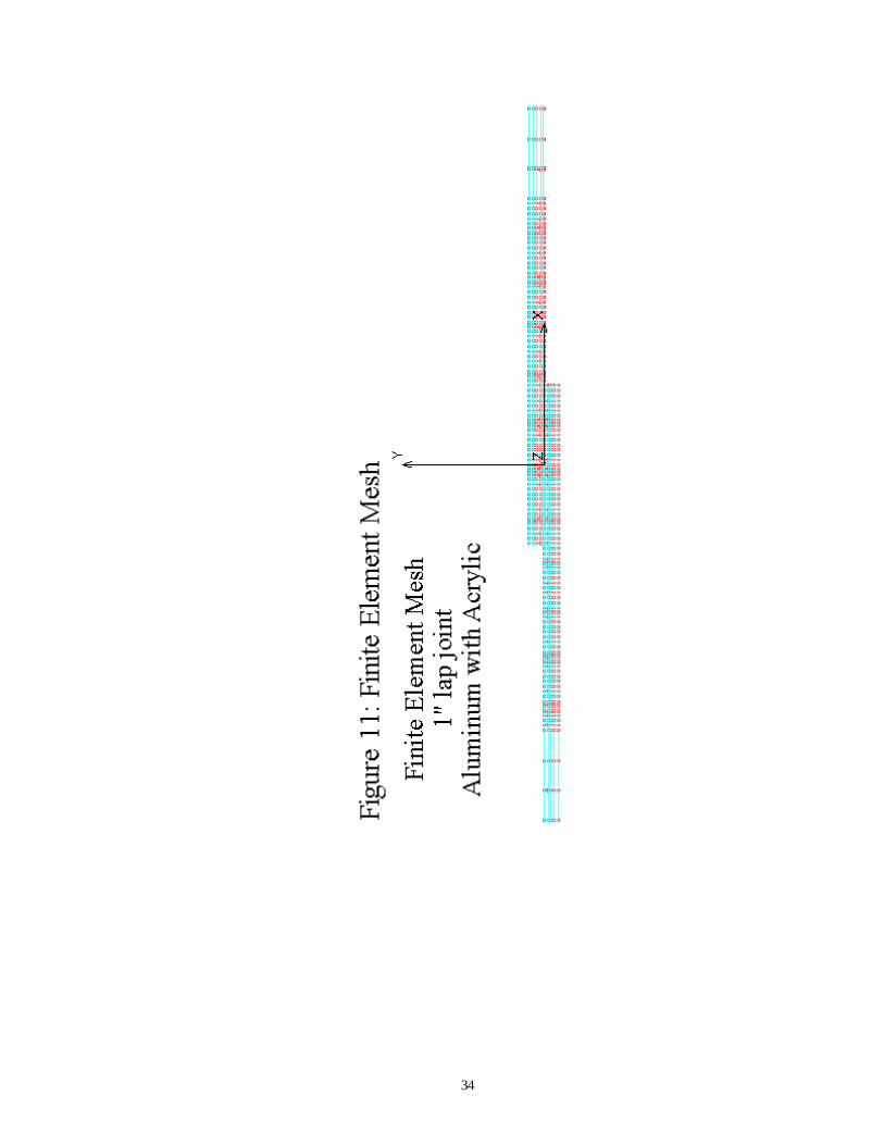
The lap joints to be tested were modeled with COSMOS. The X- and Y- axes

were scaled to the model, while the Z-axis was shortened, see Figure 11. This was done

since the strains were uniform along the Z-axis Geometrical objects were created by the

computer program using points, surfaces, and volumes. These were then meshed

(connected) such that the adhesive areas and those areas of aluminum near the adhesive

also had denser meshes to accommodate areas of interest. All rotations of the part were

fixed at zero, as were the Y- and Z- displacements at both ends of the joint. The line of

nodes through the center of the joint was used to fix the center of the lap joint. Each node

in this line was fixed. Loads were applied at each end to simulate the effects of the load

frame. The models were then analyzed with the applied loads and the theoretical strains

were obtained. Appendix A contains the COSMOS commands used to generate the

models.

34

35

36

37

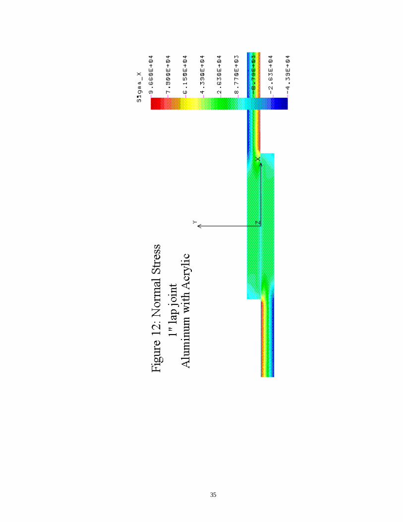
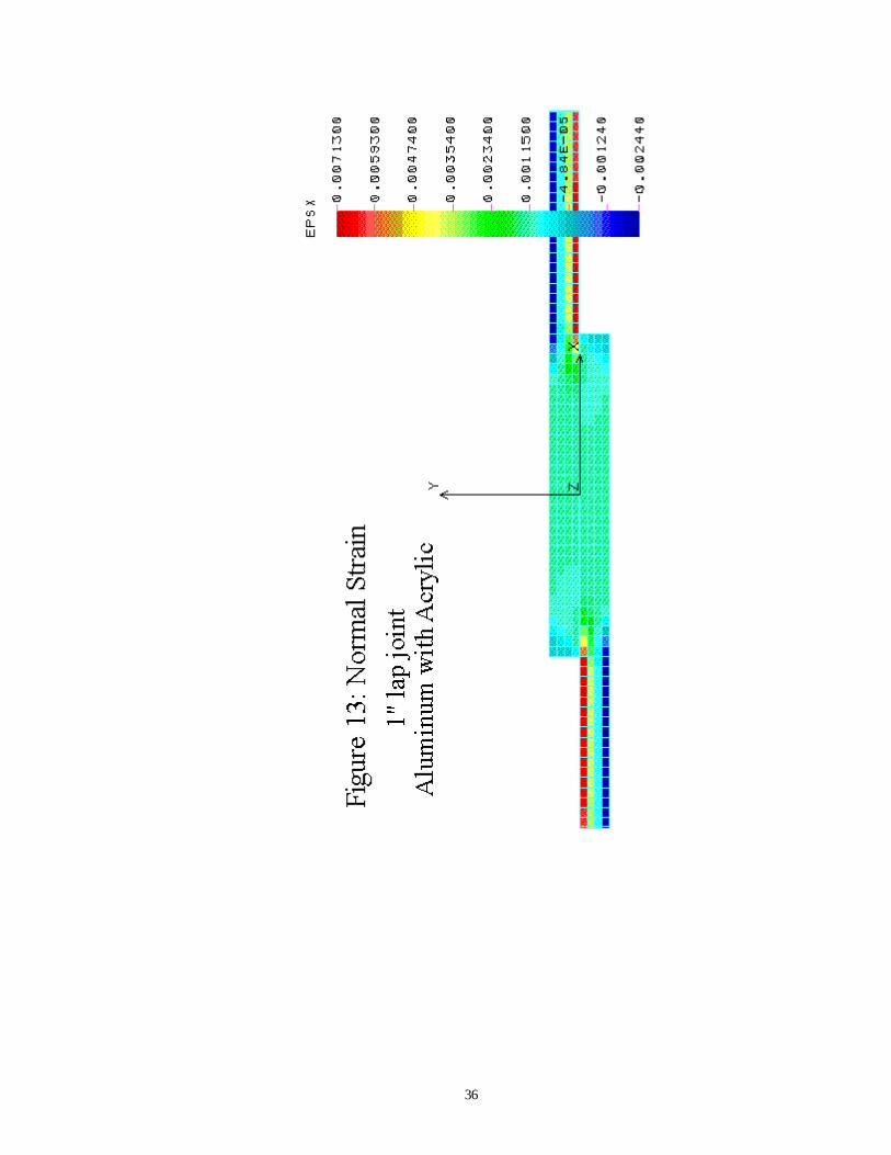
Examples of finite element models of lap joints can be found in Figures 11-13. In

Figure 11, the mesh is shown. A dense mesh was used in the area of the adhesive bond

since that was the area of interest. This provided more information in the area of the

bond. Figure 12 shows the normal stress along the X-axis. The highest areas of tension

(in red) were at the overlap corners. In Figure 13, the high strain concentrations

correspond to the areas of high stress.

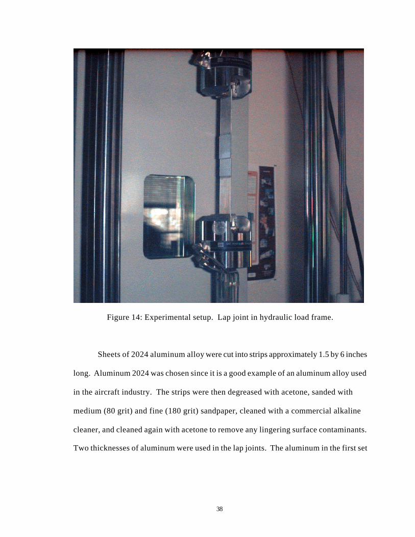
IV. EXPERIMENT

Aluminum lap joints were fabricated and coated with a polycarbonate photoelastic

material to test for changes in the surface fringe pattern indicative of plastic deformation.

The samples were tested in tension in a hydraulic load frame (810 Material Test System),

shown in Figure 14. The optical fringes on the surfaces of the joints were observed and

correlated with the results of a finite element model calculation. The goal of this was to

compare the strains derived from the fringes to the strains in the finite element models.

Comparison verified that the finite element calculations reflected reality.

38

Figure 14: Experimental setup. Lap joint in hydraulic load frame.

Sheets of 2024 aluminum alloy were cut into strips approximately 1.5 by 6 inches

long. Aluminum 2024 was chosen since it is a good example of an aluminum alloy used

in the aircraft industry. The strips were then degreased with acetone, sanded with

medium (80 grit) and fine (180 grit) sandpaper, cleaned with a commercial alkaline

cleaner, and cleaned again with acetone to remove any lingering surface contaminants.

Two thicknesses of aluminum were used in the lap joints. The aluminum in the first set

39

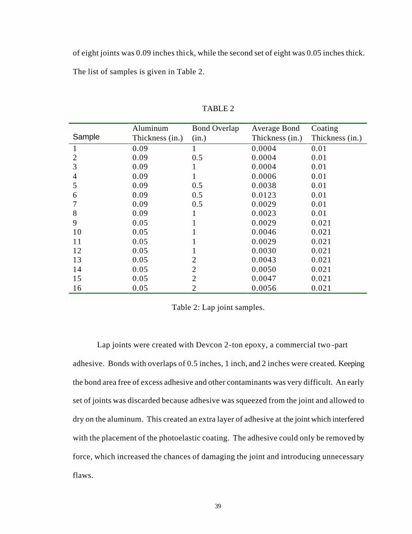
of eight joints was 0.09 inches thick, while the second set of eight was 0.05 inches thick.

The list of samples is given in Table 2.

TABLE 2

Sample Aluminum Thickness (in.)

Bond Overlap (in.)

Average Bond Thickness (in.)

Coating Thickness (in.)

1 0.09 1 0.0004 0.01 2 0.09 0.5 0.0004 0.01 3 0.09 1 0.0004 0.01 4 0.09 1 0.0006 0.01 5 0.09 0.5 0.0038 0.01 6 0.09 0.5 0.0123 0.01 7 0.09 0.5 0.0029 0.01 8 0.09 1 0.0023 0.01 9 0.05 1 0.0029 0.021 10 0.05 1 0.0046 0.021 11 0.05 1 0.0029 0.021 12 0.05 1 0.0030 0.021 13 0.05 2 0.0043 0.021 14 0.05 2 0.0050 0.021 15 0.05 2 0.0047 0.021 16 0.05 2 0.0056 0.021

Table 2: Lap joint samples.

Lap joints were created with Devcon 2-ton epoxy, a commercial two -part

adhesive. Bonds with overlaps of 0.5 inches, 1 inch, and 2 inches were created. Keeping

the bond area free of excess adhesive and other contaminants was very difficult. An early

set of joints was discarded because adhesive was squeezed from the joint and allowed to

dry on the aluminum. This created an extra layer of adhesive at the joint which interfered

with the placement of the photoelastic coating. The adhesive could only be removed by

force, which increased the chances of damaging the joint and introducing unnecessary

flaws.

40

After the joints were created, a photoelastic coating was added to the top of each

joint. Flat coatings are used for flat surfaces, while contoured coatings are available for

other geometries. In the present case, a flat PS-1 coating was bonded with a two -part

adhesive to the lap joints in the region of the overlap and extending toward the ends of

the sample by approximately 1.5 inches.

Coating edges needed to be matched with edges adjacent and perpendicular to the

test part edges. Holes drilled for bolts, rivets, and test part seams should be located

between sheets. This is especially important around holes or discontinuities since they

exhibit higher stress concentrations. Holes and seams were not applicable in the present

research [10].

The photoelastic sheets used in this application were preformed flat sheets with a

reflective backing on one side. The sheets were cut with a sharp blade to reduce the

introduction of additional stresses, chips or cracks in the coating causing unwanted

fringes that interfere with the desired photoelastic fringes. Cleaning of the PS-1 coating

was only done with isopropyl alcohol [10].

Photoelastic adhesive, a mixture of a resin and hardener, was applied to the test

surface to bond the optical coating. The chosen adhesive for the photoelastic sheets on

the lap joints was the PC-1 (resin) with PCH-1 (hardener). Prior to mixing, it was

necessary to calculate the surface area to be covered, which gave the grams of mixed

adhesive needed. One gram of mixed adhesive covered about 10 cm2, 1 mm thick. The

resin was heated to 90°F (32°C) and ten parts per hundred of the hardener by weight were

added to the resin. The hardener (PCH-1) was added at room temperature. No more than

100 grams of adhesive could be mixed per batch since amounts larger than this

41

significantly decreased pot life. The parts were mixed until the adhesive was non-

streaking and homogeneous, about 3 to 5 minutes. Upon application, any excess

adhesive was squeezed out, leaving a final layer 0.1 to 0.25 mm thick. Finally, the bond

was cured for 12 hours at room temperature.

Normal adhesive bonding procedures should be followed to obtain the optimum

photoelastic adhesive bond. The area should be clean with a temperature of 65-85°F (18-

29°C). Masking tape should be applied about 3/16 inches from the boundaries of the

photoelastic coating. The adhesive is brushed over the aluminum surface to a thickness

of at least 1 mm. The coating is applied by pressing down on the top, starting at edge and

working across with constant pressure to press out any air. The coating should be pressed

again after it is applied to bleed out any additional adhesive. The paper backing should

still be on the coating to preclude damage of the photoelastic coating. Adhesive needs to

be brushed at the edges of the coating to seal against air and moisture. A final adhesive

thickness of 0.01 to 0.03 mm is typical. If the coating slides upon application, it can be

tacked in place with masking tape. It will then be allowed to set for one to two hours. At

this point, the tape is r emoved. All excess adhesive must also be removed at this time, as

should the paper backing on the coating. The adhesive must cure for twelve hours before

testing [10].

The 0.09-inch joints yielded little photoelastic information. Two of the eight

0.09-inch samples broke before testing began because of compression by the load frame.

Very little photoelastic signal was seen from the other 0.09-inch samples. This could be

due to a dim light source or the metal could have been too thick to see significant strains.

The photoelastic coating was 0.010 inches thick. The next set of samples was made from

42

0.05 inch aluminum with one- and two- inch overlaps. These were coated with a 0.021

inch photoelastic coating. A brighter flashlight was used as the light source for visual

measurements.

Testing with the 810 Material Test System (MTS) load frame was performed by

writing a procedure to ramp up the force by 100 N per second to the final load, hold for

30 seconds, and ramp down to 0 N. Before each run, the desired force is changed in the

procedure. The procedure was written with TestStar II, a commercial software package.

At any point, the machine may be manually “held” at a load and then released. After the

sample was loaded and held with the grips, the procedure could begin. As the force was

held constant, photoelastic measurements were taken with flashlight and polarizing

filters. Digital photographs were also taken for archival purposes. The digital camera

had a flash brighter than the flashlight used in the visual measurements.

Circularly polarized light was reflected from the coating, and the resulting fringe

patterns were then viewed with a reflection polariscope of flashlight and filters. Some

images were captured with a digital camera with filters over the flash and lens. The

fringe patterns started at the bond line and extended out toward the ends from there.

These strain distributions correlated with the strain distributions in the finite element

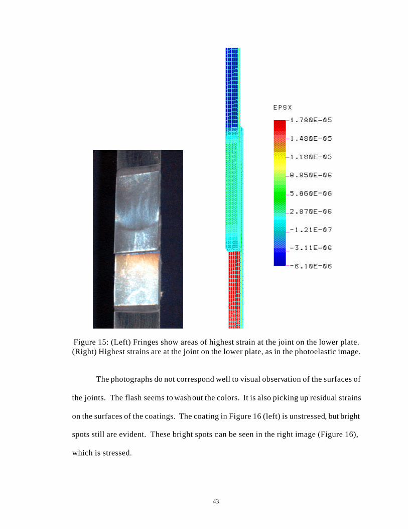
models, as in Figure 15.

43

Figure 15: (Left) Fringes show areas of highest strain at the joint on the lower plate. (Right) Highest strains are at the joint on the lower plate, as in the photoelastic image.

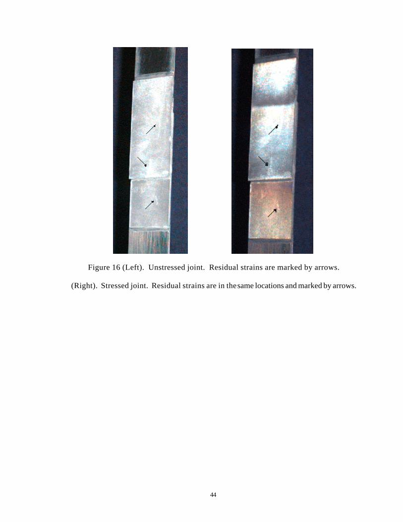
The photographs do not correspond well to visual observation of the surfaces of

the joints. The flash seems to wash out the colors. It is also picking up residual strains

on the surfaces of the coatings. The coating in Figure 16 (left) is unstressed, but bright

spots still are evident. These bright spots can be seen in the right image (Figure 16),

which is stressed.

44

Figure 16 (Left). Unstressed joint. Residual strains are marked by arrows.

(Right). Stressed joint. Residual strains are in the same locations and marked by arrows.

45

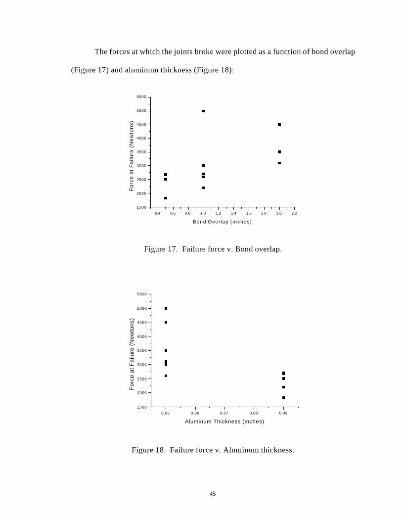
The forces at which the joints broke were plotted as a function of bond overlap

(Figure 17) and aluminum thickness (Figure 18):

0.4 0.6 0.8 1.0 1.2 1.4 1.6 1.8 2.0 2.2

1500

2000

2500

3000

3500

4000

4500

5000

5500

Fo

rce

at

Fa

ilure

(N

ew

ton

s)

Bond Over lap ( inches)

Figure 17. Failure force v. Bond overlap.

0.05 0.06 0.07 0.08 0.09

1500

2000

2500

3000

3500

4000

4500

5000

5500

Fo

rce

at

Fa

ilure

(N

ew

ton

s)

Aluminum Thickness (inches)

Figure 18. Failure force v. Aluminum thickness.

46

Purple was the first color to appear on the test surface. The samples should start

with black and go through gray, white, yellow, orange, and a dull red before getting to

purple. In addition, no complete fringe pattern ever appeared on the surface. As new

fringes appeared, the older ones should get pushed out to the edges, as expected, but

without the early colors. This may have been because the sample was only partially

coated and these areas of lower stress were not on the coated area. While the fringes

appeared in the correct order, they did not seem to represent a readily identifiable fringe

pattern since they only exhibited purple through red. See Table 1 for the color sequence.

The light source may have been too dim to observe the early colors.

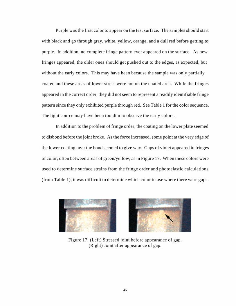
In addition to the problem of fringe order, the coating on the lower plate seemed

to disbond before the joint broke. As the force increased, some point at the very edge of

the lower coating near the bond seemed to give way. Gaps of violet appeared in fringes

of color, often between areas of green/yellow, as in Figure 17. When these colors were

used to determine surface strains from the fringe order and photoelastic calculations

(from Table 1), it was difficult to determine which color to use where there were gaps.

Figure 17: (Left) Stressed joint before appearance of gap. (Right) Joint after appearance of gap.

47

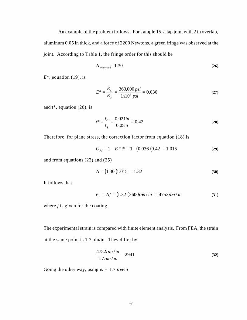
An example of the problem follows. For s ample 15, a lap joint with 2 in overlap,

aluminum 0.05 in thick, and a force of 2200 Newtons, a green fringe was observed at the

joint. According to Table 1, the fringe order for this should be

30.1=observedN (26)

E*, equation (19), is

036.0101

000,360*

6===

psixpsi

EE

ES

C (27)

and t*, equation (20), is

42.005.0021.0

* ===inin

tt

tS

C (28)

Therefore, for plane stress, the correction factor from equation (18) is

( )( ) 015.142.0036.01**1 =+=+= tECPS (29)

and from equations (22) and (25)

( )( ) 32.1015.130.1 ==N (30)

It follows that

( )( ) ininininNfx /4752/360032.1 µµε === (31)

where f is given for the coating.

The experimental strain is compared with finite element analysis. From FEA, the strain

at the same point is 1.7 µin/in. They differ by

2941/7.1

/4752 =inininin

µµ

(32)

Going the other way, using εx = 1.7 µin/in

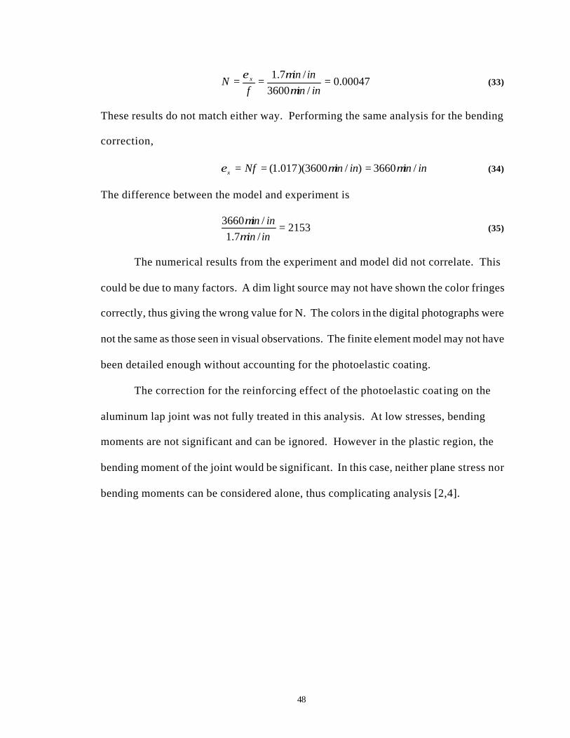
48

00047.0/3600

/7.1 ===inin

ininf

N x

µµε

(33)

These results do not match either way. Performing the same analysis for the bending

correction,

ininininNfx /3660)/3600)(017.1( µµε === (34)

The difference between the model and experiment is

2153/7.1

/3660 =inininin

µµ

(35)

The numerical results from the experiment and model did not correlate. This

could be due to many factors. A dim light source may not have shown the color fringes

correctly, thus giving the wrong value for N. The colors in the digital photographs were

not the same as those seen in visual observations. The finite element model may not have

been detailed enough without accounting for the photoelastic coating.

The correction for the reinforcing effect of the photoelastic coat ing on the

aluminum lap joint was not fully treated in this analysis. At low stresses, bending

moments are not significant and can be ignored. However in the plastic region, the

bending moment of the joint would be significant. In this case, neither plane stress nor

bending moments can be considered alone, thus complicating analysis [2,4].

49

V. CONCLUSION

The location of strain distributions in the photoelastic measurements correspond

to strain distribution locations in the finite element analysis. At the moment, however, it

seems that the photoelastic coating is failing around the point of failure of the joint, but it

is unclear how the coating is affecting the joint strength of the aluminum lap joint. It is

possible that the stiffening effect of the photoelastic coating allows the joint to carry a

higher load, but once the photoelastic adhesive bond breaks, the forces are too great for

the joint to carry and it fails. The coatings are known to have reinforcing effects and the

moduli of elasticity for the epoxy, plastic coating, and photoelastic adhesive are all within

the same order of magnitude. Young’s modulus of the Type PS-1 polycarbonate coating

is approximately 360,000 psi [4]. The modulus of elasticity for the photoelastic adhesive

is about 450,000 psi [10]. It is about 350,000 psi for the joint (if the epoxy is

approximated by a medium-high impact acrylic). The problem is quite complicated and

needs much more attention.

50

VI FUTURE WORK

Much work is necessary before photoelasticity can be used to evaluate lap joints.

American Society of Testing Materials standards for bonding could be followed to obtain

more uniform bonds for testing. Also, an adhesive with a modulus of elasticity

significantly lower than that of the photoelastic coating would be certain to fail first,

thereby avoiding having two moduli of elasticity which are almost the same. However,

this would not be representative of structural bonds. Other coatings could also be tried on

the surface, including coatings which could be applied like paint [8]. Within the finite

element models, the extra adhesive layers from the photoelastic coating could be added

for analysis. Additionally, a finer mesh could be used for the models in an attempt to

gain more information about the bonds.

ACKNOWLEDGEMENTS

The author would like to thank Dr. Mark Hinders for his guidance on this project,

as well as Mrs. Deonna Woolard for her help and support. Thanks also to Mr. Jesse

Becker for many helpful discussions.

51

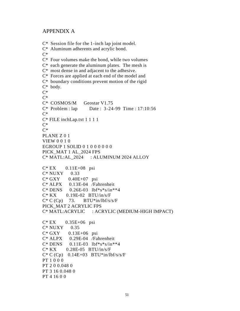
APPENDIX A

C* Session file for the 1-inch lap joint model. C* Aluminum adherents and acrylic bond. C* C* Four volumes make the bond, while two volumes C* each generate the aluminum plates. The mesh is C* most dense in and adjacent to the adhesive. C* Forces are applied at each end of the model and C* boundary conditions prevent motion of the rigid C* body. C* C* C* COSMOS/M Geostar V1.75 C* Problem : lap Date : 3-24-99 Time : 17:10:56 C* C* FILE inchLap.txt 1 1 1 1 C* C* PLANE Z 0 1 VIEW 0 0 1 0 EGROUP 1 SOLID 0 1 0 0 0 0 0 0 PICK_MAT 1 AL_2024 FPS C* MATL:AL_2024 : ALUMINUM 2024 ALLOY C* EX 0.11E+08 psi C* NUXY 0.33 C* GXY 0.40E+07 psi C* ALPX 0.13E-04 /Fahrenheit C* DENS 0.26E-03 lbf*s*s/in**4 C* KX 0.19E-02 BTU/in/s/F C* C (Cp) 73. BTU*in/lbf/s/s/F PICK_MAT 2 ACRYLIC FPS C* MATL:ACRYLIC : ACRYLIC (MEDIUM-HIGH IMPACT) C* EX 0.35E+06 psi C* NUXY 0.35 C* GXY 0.13E+06 psi C* ALPX 0.29E-04 /Fahrenheit C* DENS 0.11E-03 lbf*s*s/in**4 C* KX 0.28E-05 BTU/in/s/F C* C (Cp) 0.14E+03 BTU*in/lbf/s/s/F PT 1 0 0 0 PT 2 0 0.048 0 PT 3 16 0.048 0 PT 4 16 0 0

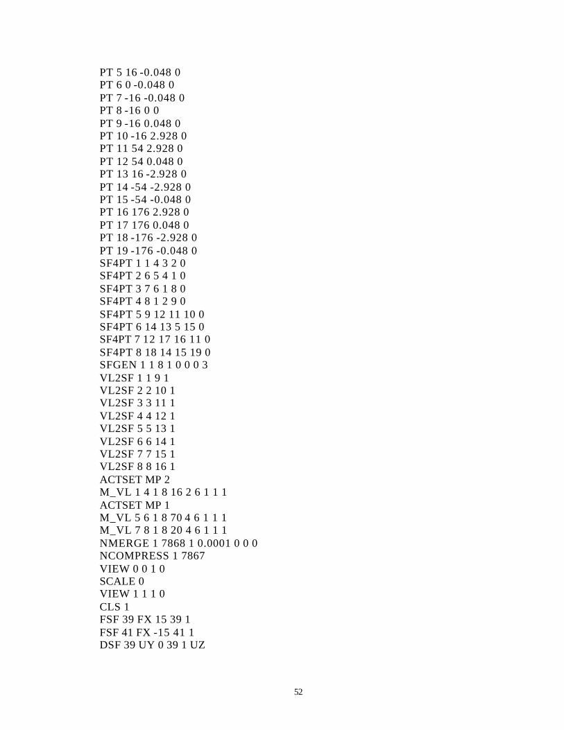
52

PT 5 16 -0.048 0 PT 6 0 -0.048 0 PT 7 -16 -0.048 0 PT 8 -16 0 0 PT 9 -16 0.048 0 PT 10 -16 2.928 0 PT 11 54 2.928 0 PT 12 54 0.048 0 PT 13 16 -2.928 0 PT 14 -54 -2.928 0 PT 15 -54 -0.048 0 PT 16 176 2.928 0 PT 17 176 0.048 0 PT 18 -176 -2.928 0 PT 19 -176 -0.048 0 SF4PT 1 1 4 3 2 0 SF4PT 2 6 5 4 1 0 SF4PT 3 7 6 1 8 0 SF4PT 4 8 1 2 9 0 SF4PT 5 9 12 11 10 0 SF4PT 6 14 13 5 15 0 SF4PT 7 12 17 16 11 0 SF4PT 8 18 14 15 19 0 SFGEN 1 1 8 1 0 0 0 3 VL2SF 1 1 9 1 VL2SF 2 2 10 1 VL2SF 3 3 11 1 VL2SF 4 4 12 1 VL2SF 5 5 13 1 VL2SF 6 6 14 1 VL2SF 7 7 15 1 VL2SF 8 8 16 1 ACTSET MP 2 M_VL 1 4 1 8 16 2 6 1 1 1 ACTSET MP 1 M_VL 5 6 1 8 70 4 6 1 1 1 M_VL 7 8 1 8 20 4 6 1 1 1 NMERGE 1 7868 1 0.0001 0 0 0 NCOMPRESS 1 7867 VIEW 0 0 1 0 SCALE 0 VIEW 1 1 1 0 CLS 1 FSF 39 FX 15 39 1 FSF 41 FX -15 41 1 DSF 39 UY 0 39 1 UZ

53

DSF 41 UY 0 41 1 UZ DCR 53 UX 0 53 1 C* R_STATIC C* C* COSMOS/M Geostar V1.75 C* Problem : lap Date : 3-24-99 Time : 17:19:44 C* C* R_STATIC C* C* COSMOS/M Geostar V1.75 C* Problem : lap Date : 3-24-99 Time : 17:32:45 C* VIEW 0 0 1 0 VIEW 0 0 1 0 VIEW 1 1 1 0 VIEW 0 0 1 0

54

REFERENCES

1. D. Hagemaier. “Adhesive -Bonded Joints.” ASM Handbook, 17, pp. 610-640 (1989).

2. R. Messler, Jr. Joining of Advanced Materials (Butterworth-Heinemann,

Massachusetts, 1993).

3. “Introduction to Stress Analysis by the PhotoStress Method,” Measurements Group

Tech Notes TN-702-1, Measurements Group, Inc., Raleigh, North Carolina. 1989.

4. “Principal Stress Separation in PhotoStress Measurements,” Measurements Group

Tech Notes TN-708-1, Measurements Group, Inc., Raleigh, North Carolina. 1992.

5. “The Lotus Position,”

http://www.sandsmuseum.com/cars/elise/press/technical/engalu.html. 4/15/1999.

6. G.M. Light and H. Kwan. Nondestructive Evaluation of Adhesive Bond Quality.

(Nondestructive Testing Information Analysis Center, Texas, 1989).

7. C.C. Spyrakos. Finite Element Modeling in Engineering Practice. (West Virginia

University Press, West Virginia, 1994).

8. D.J. Woolard and M.K. Hinders. “Coatings for Combined Thermoelastic and

Photoelastic Stress Measurement,” to appear in “Nondestructive Evaluation of

Bridges and Highways.” Steven Chase, ed. SPIE, vol. 3587, (1999).

9. R.C. Hibbeler. Statics and Mechanics of Materials. (Macmillan Publishing

Company, New York, 1992).

10. “Instructions for Bonding Flat and Contoured Photoelastic Sheets to Test-Part

Surfaces,” Measurements Group Tech Notes IB-223-G, Measurements Group, Inc.,

Raleigh, North Carolina. 1982.

55

11. D.F. Weyher, Supervisor. Adhesives in Modern Manufacturing. (Society of

Manufacturing Engineers, Michigan, 1970).

12. D. Falk, D. Brill, and D. Stork. Seeing the Light; Optics in Nature, Photography,

Color, Vision, and Holography. (John Wiley & Sons, New York, 1986).

13. D. Logan. A First Course in the Finite Element Method. (PWS Engineering, Boston,

1986).

14. G. Strang. Introduction to Applied Mathematics. (Wellesley-Cambridge Press,

Massachusetts, 1986).