NONCONTRACTIBLE HETEROGENEITY IN

DIRECTED SEARCH

MICHAEL PETERS,DEPARTMENT OF ECONOMICS,

UNIVERSITY OF BRITISH COLUMBIA

Abstract. This paper provides a directed search model designedto explain the residual part of wage variation left over after theimpact of education and other observable worker characteristicshas been removed. Workers have private information about theircharacteristics at the time they apply for jobs. Firms value thesecharacteristics differently and can observe them once workers ap-ply. They hire the worker they most prefer. However, the charac-teristics aren’t contractible, so firms can’t condition their wages onthem. The paper shows how to extend arguments from directedsearch to handle this, allowing for arbitrary distributions of workerand firm types. The model is used to provide a functional relation-ship that ties together the wage distribution and the wage-durationfunction. This relationship provides a testable implication of themodel. This relationship suggests a common property of wagedistributions that guarantees that workers who leave unemploy-ment at the highest wages also have the shortest unemploymentduration. This is in strict contrast to the usual (and somewhatimplausible) directed search story in which high wages are alwaysaccompanied by higher probability of unemployment.

1. Introduction

This paper provides a directed search model in which worker andfirm characteristics differ, but where firms cannot cannot conditionthe wages they pay on worker characteristics as they can in paperslike in (Shi 2002) or (Shimer 2005). Examples of such characteristicsmight be things like reference letters that convey a lot of informationabout an applicants skill as long as they are not contractible. Anotherexample might be connections and friendships that workers have withmanagers, or just with other workers in the industry. These connectionstypically cannot be verified in any way that would be satisfactory ina formal contract. Alternatively, firms may care a lot about worker

I am grateful to Daron Acemoglu, Rob Shimer and a number of referees for lot ofsubstantive and expositional help. The work on this paper was funded by SSHRC..

1

characteristics on which they aren’t allowed to condition wages - forexample whether or not the worker has a criminal record, or a historyof union activism.

Workers know their own characteristics at the time they apply forjobs, but they don’t know the characteristics of other workers whomight apply. Firms value these characteristics differently and can ob-serve these characteristics once workers apply. Once they have collecteda bunch of applications, they hire the worker they most prefer.

The paper shows how to extend directed search to handle this, allow-ing for arbitrary distributions of worker and firm types. More broadly,this approach provides a method to understand the variation in wagesthat cannot be attributed to observable characteristics. The basic logicof the model ties together the wage distribution and the unemploymentduration function, i.e., the relationship between the wage at which aworker leaves unemployment, and his duration. This relationship pro-vides a potentially testable implication of the model.

The relationship between the wage duration function and the wagedistribution developed in this paper makes it possible to examine oneof the key predictions of directed search in models where wages can’tbe conditioned on worker type - workers who submit applications tohigh wage firms should expect to be hired by those firms with lowprobability.1 There isn’t a lot of evidence about this central prediction,however, what there is doesn’t seem to support it. Addison, Centeno,and Portugal (2004), for example, provide some evidence to suggestthat the wages at which workers leave unemployment and the durationof their unemployment spell are negatively correlated. The evidence isnot strong, but it certainly provides no support at all for the classicalprediction of directed search.2

1For example (Peters 2000), (Lang, Manove, and Dickens 1999), (Eeckhout andKircher 2008),(Acemoglu and Shimer 2000) or (Shi 2009) all generate equilibriumwage dispersion for which wage and employment probability are related in this way.Of course, when wages can be made conditional on type, as in (Shi 2002) or (Shimer2005), workers who receive higher wages are being compensated for having a morevaluable type, not for bearing risk, so no such relationship would be expected inthese models.

2Many models of directed search assume that workers and firms are identical, sothis assertion isn’t so much a prediction as it is a statement about what happens outof equilibrium. However, there are many models that support distributions of wagesin equilibrium. For example, Shi (2002), Shimer (2005) and (Lang, Manove, andDickens 1999) all allow for a finite number of different types of workers. In (Peters2000) workers are identical, but there is a continuum of different types of firms. InDelacroix and Shi (2006) and (Shi 2009), workers equilibrium wages (and searchstrategies) depend on their employment history. Albrecht, Gautier, and Vroman

2

The argument below illustrates that the relationship between wageand unemployment duration is driven by two considerations. The firstis completely intuitive - higher wage firms will tend to hire workerswhose (externally unobservable) quality is higher, and these workerswill tend to be more likely to find jobs no matter where they apply. Thiscreates a positive relationship between quality, employment probabilityand wage. This is confounded by the fact that higher quality workerswill tend to use different application strategies than low quality workers.In particular, they will tend to apply at high wage jobs along with alot of other high quality workers. This effect leads in the oppositedirection, lowering the probability with which high quality workers willbe hired. This is where the directed search model plays a role sinceit ties down the application strategy for workers of different qualities.The characterization of the equilibrium application strategy provides atestable connection between wage offer distribution and the durationfunction. One implication of this relationship is that it provides arelatively simple (and apparently normally satisfied) restriction on thewage distribution that ensures that workers who leave unemploymentat high wages tend to have shorter unemployment spells.

The paper begins with an analysis of the case where there is a con-tinuum of workers and firms. The actions of individual firms support awage offer distribution. Workers’ decisions support a joint distributionof applications across wages and types. The payoff functions resemblethose in a standard directed search model. Yet there is an importantdifference. Instead of being concerned with the expected number ofcompetitors he will face when he applies at a given wage, a worker isinstead concerned with the expected number of competitors with highertypes.

For this reason, firms who set high wages don’t necessarily get moreapplicants than low wage firms. However, the average quality of theapplicant they receive is higher and this compensates them for thehigher wages they commit themselves to pay. If firms differ in the waythey value worker quality on the margin, then firms who like workerquality will set higher wages. This will induce an imperfect matchingof high quality workers with firms who value that quality.

However, we show that this matching will be imperfect. The reasonis that equilibrium application strategies will have workers acting as if

(2006) or Galenianos and Kircher (2005) support wage distributions by allowingmultiple applications. Finally, other than the model described in the paper, theonly one I am familiar with that allows a continuum of both firm and worker typesis (Eeckhout and Kircher 2008). In all these models, the standard tradeoff betweenhigh wages and low employment probabilities occurs on the equilibrium path.

3

they were following a ’reservation wage rule’ in which they apply withequal probability to all firms who set wages above their reservationwage. For this reason mismatches will continue, with high value em-ployees remaining unemployed simply because they tried to competewith other high quality employees and high producitivity firms fill-ing vacancies with low quality workers simply because no high qualityworkers apply.

We provide a pair of functional equations that can be used to charac-terize the equilibrium wage distribution and the equilibrium applicationstrategy of workers. We use these to illustrate the equilibrium with anumber of examples and to provide a condition that can be used to testthe model. We also revisit the relationship mentioned above betweenunemployment duration and exit wage. From the arguments above, itshould be apparent that exit wages induce a selection bias - workerswho leave unemployment at high wages tend to be higher type workerswho don’t compete with the lower quality applicants who also applyto high wage firms. As a consequence, there is no reason for them toexperience long unemployment spells. We use the functional equationsto compute the relationship between exit wage and average duration.In general this relationship isn’t systematic. However, we provide a re-striction on the wage distribution that ensures that workers who leaveunemployment at higher wages actually have higher employment prob-abilities.

In the final part of the paper, we focus on a micro foundation for themodel. This argument justifies the particular payoffs used in the mainpart of the paper. It also illustrates the result that workers shouldfollow a reservation wage strategy in choosing where to apply. Weconsider a finite array of firms and wages and imagine a finite numberof workers with privately knows types who apply to these firms. Wecharacterize the unique symmetric Bayesian equilibrium applicationstrategy for workers. As mentioned, it involves a reservation wage,then a set of application probabilities with which workers apply tohigher wage firms. As might be expected, the higher the wage (or thefarther away it is from the worker’s reservation wage) the lower theprobability that the worker applies. At that point, we explain why itis that low type workers have to apply to high wage firms with someprobability in order to support the equilibrium. This, of course, rulesout assortative matching. One useful consequence of this argument isto distinguish models like this one, where firms care about the type ofthe worker they hire, from models like (Eeckhout and Kircher 2008)where they don’t.

4

Finally, we show explicitly how the payoff functions in the Bayesianequilibrium of the finite game converge to the payoff functions we de-scribed for the continuum model in the first part of the paper as thenumber of workers and firms grows large. In particular, we show howlarge numbers appear to equalize the application probabilities acrossfirms. The limit theorems make it straightforward to show that purestrategy equilibrium of the finite search game support allocations thatconverge to the equilibrium allocations described in the first part of thepaper.

A few papers from the literature are worth mentioning to put thearguments here in context. Papers by (Shi 2002), and (Shimer 2005)resemble this one in that matching of worker and firm types is notassortative in equilibrium. They differ from this paper in that theyallow firms to set wages that are conditional on the type of the workerwho they ultimately hire. As a consequence, the logic that breaksdown assortative matching is much different than it is here. The exactdifferences are easier to explain once the details of the model have beenmade clearer, so the discussion of the differences is deferred to Section 8.The papers by (Lang, Manove, and Dickens 1999) and (Eeckhout andKircher 2008) provide directed search models that support assortativematching. In (Eeckhout and Kircher 2008) this is accomplished byhaving firms declare the profits they require rather than the wage theypay.3 This has the effect of making the wage a worker receives from afirm depend on the worker’s type. However, firms can’t control how thewage varies with worker type, and this prevents them from adjustingwages to ensure all types will want to apply. (Lang, Manove, andDickens 1999) is about racial discrimination, so there are only twodifferent types of worker, which permits assortative matching. Again,we defer discussion of this point until the model in this paper has beendescribed in more detail.

2. Fundamentals

A labor market consists of measurable sets M and N of firms andworkers respectively. We normalize the measure of the set of firmsto 1. The measure of the set of workers is assumed to be τ . Eachworker has a characteristic y contained in a closed connected inter-val Y =

[

y, y]

⊂ R+. These characteristics are observable to firms

once workers apply, but initially, they are private information to work-ers. Let F be a differentiable and monotonically increasing distribution

3Of course, they don’t model it in this crude way - they consider a model inwhich a firm sets the price that it wants from consumers.

5

function. Assume that τF (y) is the measure of workers whose type isless than or equal to y. These characteristics are assumed to be non-contractible. Firms are not able to make wages vary directly with thesecharacteristics. A worker’s payoff if he finds a job is simply the wagehe receives. If he fails to find a job, his payoff is zero. Workers are riskneutral.

Firms characteristics are drawn from a set X = [x, x]. Let H (x) bethe measure of the set of firms whose characteristics are less than orequal to x, with H (x) = 1 as described above. H is assumed integrablewith convex support. Each firm has a single job that it wants to fill.It chooses the wage that it wishes to pay the worker who fills this job.Each firm’s wage is chosen from a compact interval W ⊂ R

+. Payoffsfor firms depend on the wage they offer and on the characteristic ofthe worker they hire, and, of course, on their own characteristic. Thepayoff for every firm who hires a worker is v : W × Y × X → R wherex ∈ X is the firm’s type and y ∈ Y is the characteristic of the workerwhom she hires. It is assumed that v is continuously differentiable inall its arguments, concave in w and bounded. To maintain an orderon firm types, it is assumed that for any pair (w, y) and (w′, y′) with(w, y) ≥ (w′, y′), if v (w, y, x) ≥ v (w′, y′, x) for some type x, thenv (w, y, x′) ≥ v (w′, y′, x′) for any higher type x′ ≥ x. In words, thissingle crossing condition says that higher type firms assign a highervalue to higher type workers. Finally, a firm who doesn’t hire receivespayoff 0. We use the assumption that v (·, 0, ·) = 0 uniformly, whichmeans that not hiring is treated the same way as hiring a worker withtype 0.

3. The Market

Each firm in the market commits to a wage. As is typically assumedin directed search, each worker applies to one and only one firm. Thefirm is assumed to hire the highest type applicant who applies. It isassumed that a firm who advertises a job is committed to hire a workeras long as some worker applies even if the firm’s perceived ex post payofffrom the best worker who applies is negative.4 This assumption couldbe defended by observing that all the applicants who apply to the firmare verifiably qualified for the job being offered. A refusal to hire anyapplicant might be problematic for legal reasons, though, of course, nofirm is required to hire every qualified applicant who applies. However,the assumption is primarily intended to simplify the limit arguments

4A high type firm who sets a high wage in order to attract high type workersmight not be willing to pay a low type worker that wage.

6

given in the last section of the paper. The payoff functions in the largegame described in this section can be modified in a straightforward wayto allow firms to decide not to hire when they have applicants.

The payoffs that players receive depend on their own actions, and onthe distributions of actions taken by the other players. We specify thesepayoffs using standard arguments from directed search, then provide amicro foundation in Section 8. Let G be the wage offer distribution andP the joint distribution of applications, where P (w, y) is understoodto be the measure of the set of workers of type y or less who applyat wage w or less. We let pw (y) refer to the conditional distributionfunction that describes the measure of the set of applicants of type lessthan or equal to y who apply at wage w.

A worker of type y is always chosen over workers with lower typeswherever he applies. As a consequence, he is concerned not with thetotal number of applicants expected to apply at the firm where heapplies (the ’queue size’), but with the measure of the set of applicantswhose type is as least as large as his. This number is given by

∫ y

y

dpw (y) .

We use the familiar formula e−R y

y dpw(y) to give the probability of trade.5

This provides worker payoffs for wages in the support of G as

(3.1) U (w, y,G, P ) ≡ we−R y

y dpw(y).

For firms, let w be a wage in the support of G. The payoff fromemploying such a worker is v (w, x, y). Integrating over the set of workertypes gives expected profit

(3.2) V (w, x,G, P ) ≡

∫ y

y

v(w, y, x)e−R y

y dpw(y′)dpw (y)

for any wage in the support of G.In order to describe equilibrium, we need to define payoffs for both

workers and firms for wages that lie outside the support of G. In whatfollows, let G mean the support of G. The notation w means the highestwage in the support and w means the lowest wage in the support. Wecan now define the payoffs using an argument similar to (Acemoglu andShimer 2000). Define

ω (y) ≡ maxw∈G

we−R y

y dpw(y′).

5We show below that this expression is the limit value of the matching probabilityin a conventional urn-ball matching game.

7

The function ω (y) is monotonic and continuous, so it is differentiablealmost everywhere. We refer to ω (y) henceforth as the market payoff.We assume, as do (Acemoglu and Shimer 2000) (among others), thatapplication strategies adjust so that for any wage w′ 6∈ G all workerswhose market payoff is less than w′ receive exactly their market payoffwhen they apply at w′, while all other workers receive payoff w′. Inparticular, we assume U (w′, y, G, P ) = min [ω (y) , w′]. For each wagew′, we use the marginal distribution pw′that supports this property tocompute the firm’s profit when it offers such a wage.

To find this marginal distribution, we solve the functional equation

(3.3) w′e−R y

y dpw′ (y′) = ω (y)

on the support of pw′ .The solution for pw′ depends on whether w′ is above or below the

support of G.6 We discuss this briefly here to illustrate the method,and because the payoff for wages above the support is surprising. Inthe final part of the paper, we show that these payoffs functions arelimits of payoff functions in finite versions of the game.

Begin with the case where w′ < w (i.e., below the support). Ifw′ ≤ ω

(

y)

, then (3.3) has no solution for any y and pw′should beuniformly zero. Otherwise, (3.3) implies that

∫ y∗

y

dpw′ (y′) = log (w′) − log (ω (y)) .

The difference between the logs can be written as the integral of itsderivative. Using this fact, then changing the variable in the integrationgives

(3.4)

∫ y∗

y

dpw′ (y′) =

∫ y∗

y

ω′ (y)

ω (y)dy.

The firm’s payoff V (w′, x,G, P ) is then given by substituting (3.4) into(3.2).

When w′ strictly exceeds the highest wage in the support of G, (3.3)implies that

∫ y

y

dpw′ (y′) = log (w′) − log (w) +

∫ y

y

ω′ (y)

ω (y)dy.

This means that to satisfy the market payoff condition, the distributionpw′ must have an atom at y of size log (w′/w).

Heuristically, this means that when a firm sets a wage that is strictlyhigher than every other wage in the support of the distribution of wages,

6We leave out the case where G has a non-convex support since it is very similar.8

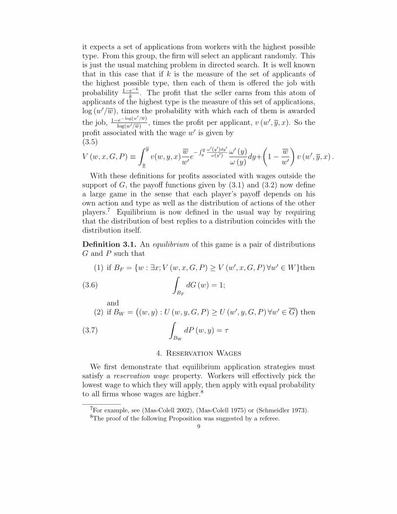
it expects a set of applications from workers with the highest possibletype. From this group, the firm will select an applicant randomly. Thisis just the usual matching problem in directed search. It is well knownthat in this case that if k is the measure of the set of applicants ofthe highest possible type, then each of them is offered the job with

probability 1−e−k

k. The profit that the seller earns from this atom of

applicants of the highest type is the measure of this set of applications,log (w′/w), times the probability with which each of them is awarded

the job, 1−e− log(w′/w)

log(w′/w), times the profit per applicant, v (w′, y, x). So the

profit associated with the wage w′ is given by(3.5)

V (w, x,G, P ) ≡

∫ y

y

v(w, y, x)w

w′e−

R yy

ω′(y′)dy′

ω(y′)ω′ (y)

ω (y)dy+

(

1 −w

w′

)

v (w′, y, x) .

With these definitions for profits associated with wages outside thesupport of G, the payoff functions given by (3.1) and (3.2) now definea large game in the sense that each player’s payoff depends on hisown action and type as well as the distribution of actions of the otherplayers.7 Equilibrium is now defined in the usual way by requiringthat the distribution of best replies to a distribution coincides with thedistribution itself.

Definition 3.1. An equilibrium of this game is a pair of distributionsG and P such that

(1) if BF = {w : ∃x; V (w, x,G, P ) ≥ V (w′, x,G, P ) ∀w′ ∈ W}then

(3.6)

∫

BF

dG (w) = 1;

and(2) if BW =

(

(w, y) : U (w, y,G, P ) ≥ U (w′, y, G, P ) ∀w′ ∈ G)

then

(3.7)

∫

BW

dP (w, y) = τ

4. Reservation Wages

We first demonstrate that equilibrium application strategies mustsatisfy a reservation wage property. Workers will effectively pick thelowest wage to which they will apply, then apply with equal probabilityto all firms whose wages are higher.8

7For example, see (Mas-Colell 2002), (Mas-Colell 1975) or (Schmeidler 1973).8The proof of the following Proposition was suggested by a referee.

9

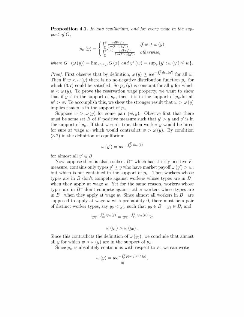
Proposition 4.1. In any equilibrium, and for every wage in the sup-port of G,

pw (y) =

{∫ y

yτdF (y′)

1−G−(ω(y′))if w ≥ ω (y)

∫ y∗(w)

yτdF (y′)

1−G−(ω(y′))otherwise,

where G− (ω (y)) = limx↑ω(y) G (x) and y∗ (w) = supy {y′ : ω (y′) ≤ w}.

Proof. First observe that by definition, ω (y) ≥ we−R y

y dpw(y′) for all w.Then if w < ω (y) there is no no-negative distribution function pw forwhich (3.7) could be satisfied. So pw (y) is constant for all y for whichw < ω (y). To prove the reservation wage property, we want to showthat if y is in the support of pw, then it is in the support of pw′for allw′ > w. To accomplish this, we show the stronger result that w > ω (y)implies that y is in the support of pw.

Suppose w > ω (y) for some pair (w, y). Observe first that theremust be some set B of F positive measure such that y′ > y and y′ is inthe support of pw. If that weren’t true, then worker y would be hiredfor sure at wage w, which would contradict w > ω (y). By condition(3.7) in the definition of equilibrium

ω (y′) = we−

R y

y′dpw(y)

for almost all y′ ∈ B.Now suppose there is also a subset B− which has strictly positive F -

measure, contains only types y′ ≥ y who have market payoff ω (y′) > w,but which is not contained in the support of pw. Then workers whosetypes are in B don’t compete against workers whose types are in B−

when they apply at wage w. Yet for the same reason, workers whosetypes are in B− don’t compete against other workers whose types arein B− when they apply at wage w. Since almost all workers in B− aresupposed to apply at wage w with probability 0, there must be a pairof distinct worker types, say y0 < y1, such that y0 ∈ B−, y1 ∈ B, and

we−

R yy0

dpw(y)= we

−R y

y1dpw(w)

≥

ω (y1) > ω (y0) .

Since this contradicts the definition of ω (y0), we conclude that almostall y for which w > ω (y) are in the support of pw.

Since pw is absolutely continuous with respect to F , we can write

ω (y) = we−R y

y p(w,y)τdF (y),10

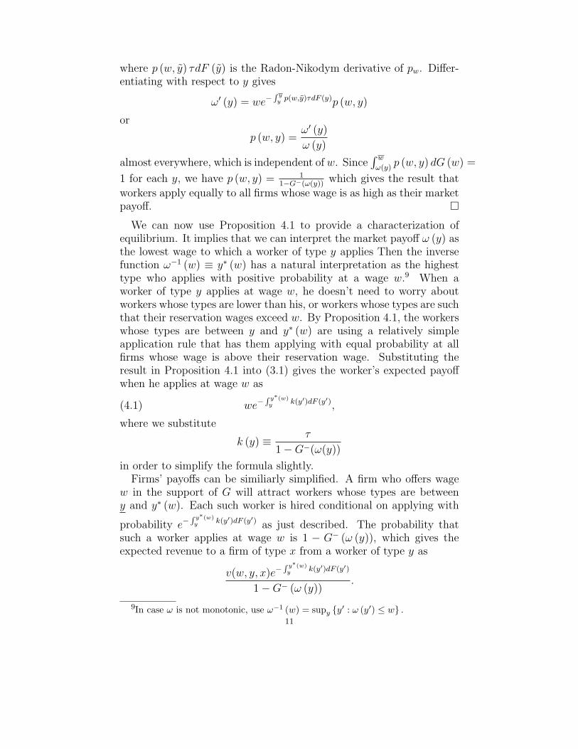
where p (w, y) τdF (y) is the Radon-Nikodym derivative of pw. Differ-entiating with respect to y gives

ω′ (y) = we−R y

y p(w,y)τdF (y)p (w, y)

or

p (w, y) =ω′ (y)

ω (y)

almost everywhere, which is independent of w. Since∫ w

ω(y)p (w, y) dG (w) =

1 for each y, we have p (w, y) = 11−G−(ω(y))

which gives the result that

workers apply equally to all firms whose wage is as high as their marketpayoff. ¤

We can now use Proposition 4.1 to provide a characterization ofequilibrium. It implies that we can interpret the market payoff ω (y) asthe lowest wage to which a worker of type y applies Then the inversefunction ω−1 (w) ≡ y∗ (w) has a natural interpretation as the highesttype who applies with positive probability at a wage w.9 When aworker of type y applies at wage w, he doesn’t need to worry aboutworkers whose types are lower than his, or workers whose types are suchthat their reservation wages exceed w. By Proposition 4.1, the workerswhose types are between y and y∗ (w) are using a relatively simpleapplication rule that has them applying with equal probability at allfirms whose wage is above their reservation wage. Substituting theresult in Proposition 4.1 into (3.1) gives the worker’s expected payoffwhen he applies at wage w as

(4.1) we−R y∗(w)

y k(y′)dF (y′),

where we substitute

k (y) ≡τ

1 − G−(ω(y))

in order to simplify the formula slightly.Firms’ payoffs can be similiarly simplified. A firm who offers wage

w in the support of G will attract workers whose types are betweeny and y∗ (w). Each such worker is hired conditional on applying with

probability e−R y∗(w)

y k(y′)dF (y′) as just described. The probability thatsuch a worker applies at wage w is 1 − G− (ω (y)), which gives theexpected revenue to a firm of type x from a worker of type y as

v(w, y, x)e−R y∗(w)

y k(y′)dF (y′)

1 − G− (ω (y)).

9In case ω is not monotonic, use ω−1 (w) = supy {y′ : ω (y′) ≤ w} .

11

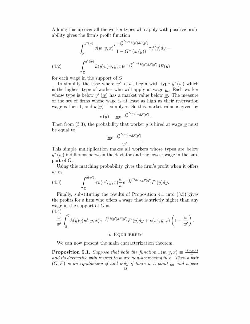
Adding this up over all the worker types who apply with positive prob-ability gives the firm’s profit function

∫ y∗(w)

y

v(w, y, x)e−

R y∗(w)y k(y′)dF (y′)

1 − G− (ω (y))τf(y)dy =

(4.2)

∫ y∗(w)

y

k(y)v(w, y, x)e−R y∗(w)

y k(y′)dF (y′)dF (y)

for each wage in the support of G.To simplify the case where w′ < w, begin with type y∗ (w) which

is the highest type of worker who will apply at wage w. Each workerwhose type is below y∗ (w) has a market value below w. The measureof the set of firms whose wage is at least as high as their reservationwage is then 1, and k (y) is simply τ . So this market value is given by

v (y) = we−R y∗(w0)

y τdF (y′).

Then from (3.3), the probability that worker y is hired at wage w mustbe equal to

we−R y∗(w0)

y τdF (y′)

w′.

This simple multiplication makes all workers whose types are belowy∗ (w) indifferent between the deviator and the lowest wage in the sup-port of G.

Using this matching probability gives the firm’s profit when it offersw′ as

(4.3)

∫ y(w′)

y

τv(w′, y, x)w

we−

R y∗(w)y τdF (y′)F ′(y)dy.

Finally, substituting the results of Proposition 4.1 into (3.5) givesthe profits for a firm who offers a wage that is strictly higher than anywage in the support of G as(4.4)

w

w′

∫ y

y

k(y)v(w′, y, x)e−R y

y k(y′)dF (y′)F ′(y)dy + v(w′, y, x)

(

1 −w

w′

)

.

5. Equilibrium

We can now present the main characterization theorem.

Proposition 5.1. Suppose that both the function ι (w, y, x) ≡ v(w,y,x)w

and its derivative with respect to w are non-decreasing in x. Then a pair(G,P ) is an equilibrium if and only if there is a point y0 and a pair

12

of functions ω (y) and h (y) satisfying ω (y0) = w, and G− (ω (y)) =H (h (y)), such that

(5.1) ω(y)τ

1 − H(h(y))F ′(y) = ω′ (y) ;

and

(5.2)

v [ω (y) , y, h (y)] = −

∫ y

y

[

vw

(

ω (y) , y′, h (y))

−v (ω (y) , y′, h (y))

ω (y)

]

ω′(

y′)

dy′.

This Proposition characterizes the equilibrium in a manner that isfamiliar in the directed search literature. The function ω is the marketpayoff function of workers, or the market utility function. The workerof type y0 breaks the set of worker types into two parts. Workers whosetypes are at or above y0 have some wage where they can apply and behired for sure. For them, the function ω (y) represents their reservationwage. The worker of type y0 in particular is sure to be hired if heapplies at the lowest wage w offered by any firm. Worker types belowy0 have a chance of losing out on the job even if they apply at the lowestwage w. The function h (y) identifies the type of the firm who offersworker y’s reservation wage when y ≥ y0, while h (y) = x if y < y0.

The two conditions can be interpreted in the usual way as tangencyconditions. For example, the payoff when a worker applies to a firm isa function of the wage that the firm offers and the highest worker typewho applies that firm. Each worker type should attain a payoff thatmaximizes this function across all wage-highest type pairs that providethe market payoff to some worker type. Equation (5.1) then expressesthe fact that a worker of type y has an indifference curve that is tangentto the market payoff function ω at y.

Similarly, interpret the firm’s profit function (4.2) as a function ofthe wage that it pays and the highest worker type it attracts. Thefirm’s problem is then to choose a wage and highest worker type thatmaximizes its profit conditional on providing some worker type hismarket payoff. The equation (5.2) expresses the requirement that aniso-profit curve for a firm of type h (y) is tangent to the market payofffunction ω (y) at the point (ω (y) , y).

It may be worth noting here that despite the tangency, this equi-librium won’t be efficient. The reason is that this allocation doesn’tdo a good job matching worker and firm types. To see this, observethat from (Shimer 2005), an efficient allocation is attained when firmscan pay workers a wage that depends on their types. Generally, a low

13

type worker who applies to a high type firm in Shimer’s model is re-warded with a lower wage than that paid to the high type workers.This focuses low type applications at low type firms, which limits mis-matching. Here a low type worker is provided the same wage as a hightype worker, providing the low type worker a much bigger incentive toapply at high wage firms. It is this concentration of applications withthe high type firms which precludes efficiency.

Proof. Start with an equilibrium pair P and G. Let w be the lowestwage in the support of G and y0 = sup {y : ω (y) ≤ w}. From Propo-sition 4.1, each worker type y must attain his market payoff ω (y) byapplying at any wage above his reserve price. So

(5.3) we−R y∗(w)

y k(y′)dF (y′) = constant

for each w ≥ ω(y). For each worker type y, the derivative of thisexpression with respect to w should then be zero at every wage aboveω (y). That is

we−R y∗(w)

y k(y′)dF (y′)k(y∗(w))F ′(y∗(w))dy∗(w)

dw= e−

R y∗(w)y k(y′)dF (y′)

giving

(5.4) wτ

1 − G−(w)F ′(y∗(w)) =

1

dy∗(w)/dw

Since y∗(w) is the inverse function of ω(y) at each point at which ω isincreasing,

(5.5) ω(y)τ

1 − G−(ω(y))F ′(y) =

dω(y)

dy

at each y ≥ y0. Fix h (y) to be the solution to G− (ω (y)) = H (h (y)).The result (5.1) then follows from the definition of h.

Now use the market payoff function defined by (5.1) and its extensionto types below y0 to simplify the firm’s profit function. The firm’s profitfunction when it sets wage w ≥ ω (y0) is given by

V (w, x,G, ω) =

∫ y∗(w)

y

k(y)v(w, y, x)ω (y)

wF ′(y)dy.

Now substituting (5.1) into the firm’s profit function gives

V (w, x,G, ω) =

∫ y∗(w)

y

v(w, y, x)ω′ (y)

wdy

Observe that choosing w, then figuring out what worker types will applyby finding the worker type who has reservation wage w is equivalent to

14

choosing the highest worker type that will apply, then setting the wageequal to that worker type’s reservation wage. Firm profits can then bewritten as functions of the highest worker type who applies as

(5.6) V (ω (y) , x,G, ω) =

∫ y

y

v(ω (y) , y′, x)ω′ (y′)

ω (y)dy′

Maximizing (5.6) with respect to y gives the first order condition

v [ω (y) , y, x] = −

∫ y

y

[

vw (ω (y) , y′, x) −v (ω (y) , y′, x)

ω (y)

]

ω′ (y′) dy′

When G is an equilibrium, the firm who offers a wage equal to workery’s reservation wage is using a best reply. Hence this condition musthold when evaluated at x = h (y) for each y ≥ y, and this gives (5.2).

To make the argument in the other direction, observe that a solutionto (5.1) holds worker payoff constant as required by the first conditionof equilibrium, provide the wage distribution is given by G (ω (y)) =H (h (y)). Hence (3.7) holds for the density p (w, y) = 1

1−G−(w). The

aggregate distribution P can then be constructed by integrating thisdensity.

From equation (4.4), it is straightforward to verify that local profitmaximization conditions hold at ω (y) whenever (5.2) holds. It is thenstraightforward to verify by brute force that second order conditionsare guaranteed by the assumption that v (w, y, x) is concave in w forevery y. The same approach verifies the second order condition at w0.

Inside the support, the condition (5.2) guarantees that the first orderconditions for profit maximization hold when every firm of type h (y)offers wage ω (y). If the second order condition fails, then the iso-profitcurve in (w, y) space for firm h (y) must cross ω at another wage. Theargument is similar whether the wage at this crossing point is higheror lower than ω (y), so suppose the crossing occurs at a higher wage.Then, firm h (y)’s iso-profit curve is strictly steeper than ω at thishigher wage w′. Yet by (5.2) there is some higher type firm x′ > h (y)whose iso-profit curve is tangent to ω at w′. Since the slope of theiso-profit curve is

−ι (w, y, x)

∫ y

yιw (w, y′, x) ω′ (y′) dy′

and this ratio is non-decreasing in x by assumption, this leads to acontradiction. ¤

In this Theorem, y0 is the highest worker type who applies to thelowest wage in the support of the equilibrium wage distribution. Condi-tion (5.1) ensures that payoffs are constant above at all wages above the

15

reservation wage. The advantage of the exponential matching functionis that a reservation wage rule that satisfies this single functional equa-tion ensures the constant payoff condition for all worker types. Thecondition (5.2) is the first order condition for profit maximization - i.e.,Vw (w, x,G, ω) = 0. The term on the left hand side of the condition isthe marginal gain associated with attracting a higher type when wageis increased. The term on the right hand side is the marginal cost ofpaying a higher wage to all the lower types.

The functional h (y) has a natural interpretation as the lowest typeof the firm who offers the reservation wage of worker y. From thetype y0 and the functional equations ω and h, the wage distribution isreadily constructed. The lowest wage in the support of the distributionis ω (y0). Then for each y > y0, G− (ω (y)) = H (h (y)).

6. Examples with Identical Firms

To begin, we will assume that all firms have the same profit function.The reason this case is amenable to analysis is because the first ordercondition (5.2) reduces to a constant profit condition that involves onlythe function ω, and a boundary condition. If we begin with a functionω that satisfies this constant profit condition, we can then find thefunction G that ensures that (5.1) is satisfied. If this function is a dis-tribution function, then we have an equilibrium with a non-degeneratewage distribution.

Example 6.1. If v (w, y, x) = 1 + αy − w for all x ∈ [x, x], thenthere is a degenerate single wage equilibrium with w = 1 + αy −∫ y

y(1 + αy′) de

−R y

y′τF ′(t)dt

.

Proof. Proposition 5.1 applies to the degenerate case since we can sety0 = y and h (y) = x. To see this, observe that if the wage distributionis degenerate at some wage w0, then all workers apply at this wage.Since y0 is the highest type who applies to the lowest wage in thesupport, the conclusion y0 = y follows. The function h (y) is supposedto be the lowest firm type who offers worker y his reservation wage.Since all firms offer the same wage, this is x. We then have triviallyfrom (5.1) ω (y) τF ′ (y) = wτF ′ (y) = ω′ (y).

The first order condition (5.2) then becomes (since G− (ω (y)) =G− (w) = 0)

v [w, y, x] = −

∫ y

y

[

vw (w, y′, x) −v (w, y′, x)

w

]

ω′ (y′) dy′.

16

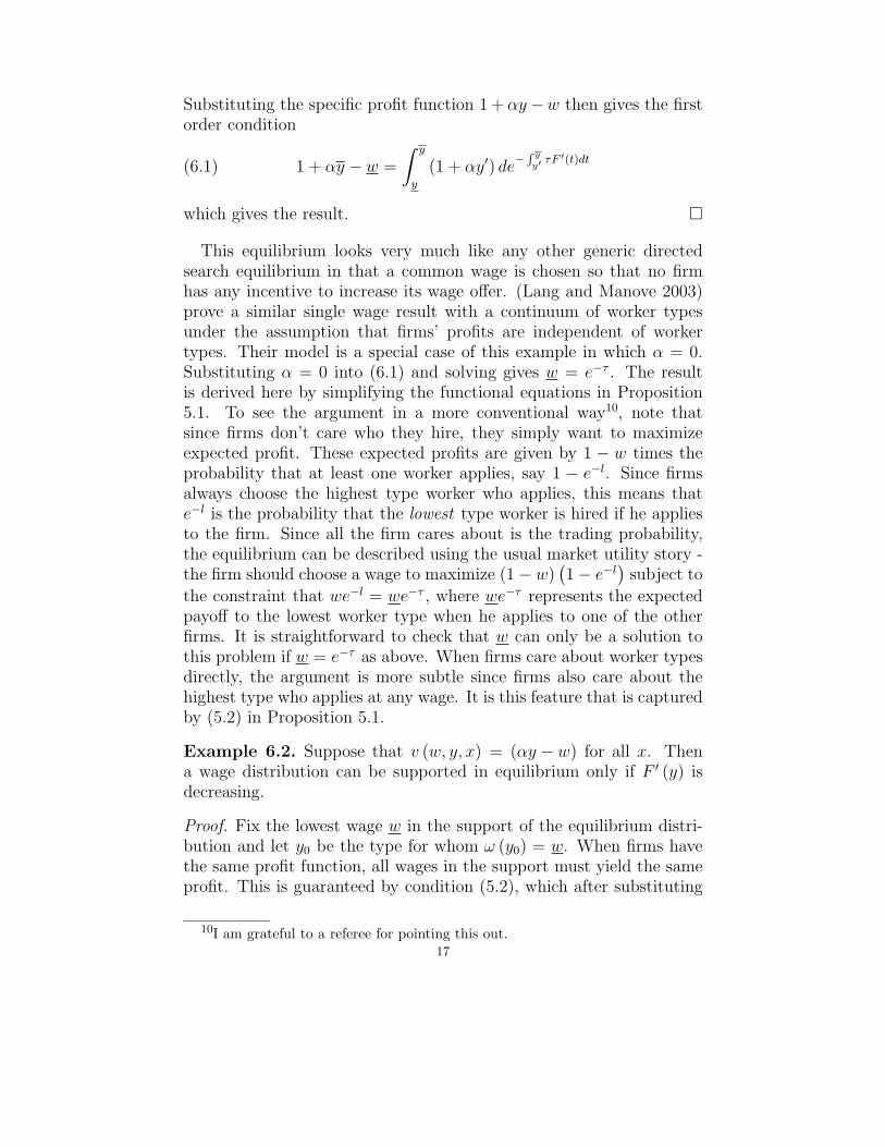
Substituting the specific profit function 1 + αy −w then gives the firstorder condition

(6.1) 1 + αy − w =

∫ y

y

(1 + αy′) de−

R y

y′τF ′(t)dt

which gives the result. ¤

This equilibrium looks very much like any other generic directedsearch equilibrium in that a common wage is chosen so that no firmhas any incentive to increase its wage offer. (Lang and Manove 2003)prove a similar single wage result with a continuum of worker typesunder the assumption that firms’ profits are independent of workertypes. Their model is a special case of this example in which α = 0.Substituting α = 0 into (6.1) and solving gives w = e−τ . The resultis derived here by simplifying the functional equations in Proposition5.1. To see the argument in a more conventional way10, note thatsince firms don’t care who they hire, they simply want to maximizeexpected profit. These expected profits are given by 1 − w times theprobability that at least one worker applies, say 1 − e−l. Since firmsalways choose the highest type worker who applies, this means thate−l is the probability that the lowest type worker is hired if he appliesto the firm. Since all the firm cares about is the trading probability,the equilibrium can be described using the usual market utility story -the firm should choose a wage to maximize (1 − w)

(

1 − e−l)

subject to

the constraint that we−l = we−τ , where we−τ represents the expectedpayoff to the lowest worker type when he applies to one of the otherfirms. It is straightforward to check that w can only be a solution tothis problem if w = e−τ as above. When firms care about worker typesdirectly, the argument is more subtle since firms also care about thehighest type who applies at any wage. It is this feature that is capturedby (5.2) in Proposition 5.1.

Example 6.2. Suppose that v (w, y, x) = (αy − w) for all x. Thena wage distribution can be supported in equilibrium only if F ′ (y) isdecreasing.

Proof. Fix the lowest wage w in the support of the equilibrium distri-bution and let y0 be the type for whom ω (y0) = w. When firms havethe same profit function, all wages in the support must yield the sameprofit. This is guaranteed by condition (5.2), which after substituting

10I am grateful to a referee for pointing this out.17

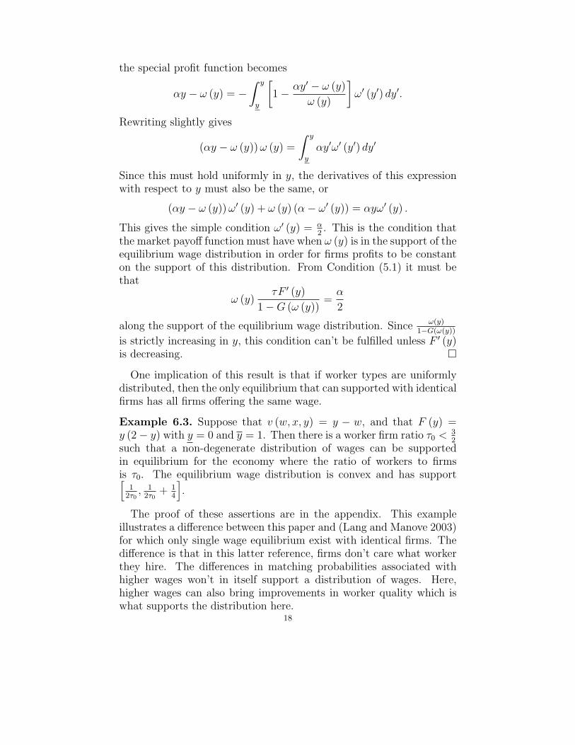
the special profit function becomes

αy − ω (y) = −

∫ y

y

[

1 −αy′ − ω (y)

ω (y)

]

ω′ (y′) dy′.

Rewriting slightly gives

(αy − ω (y)) ω (y) =

∫ y

y

αy′ω′ (y′) dy′

Since this must hold uniformly in y, the derivatives of this expressionwith respect to y must also be the same, or

(αy − ω (y)) ω′ (y) + ω (y) (α − ω′ (y)) = αyω′ (y) .

This gives the simple condition ω′ (y) = α2. This is the condition that

the market payoff function must have when ω (y) is in the support of theequilibrium wage distribution in order for firms profits to be constanton the support of this distribution. From Condition (5.1) it must bethat

ω (y)τF ′ (y)

1 − G (ω (y))=

α

2

along the support of the equilibrium wage distribution. Since ω(y)1−G(ω(y))

is strictly increasing in y, this condition can’t be fulfilled unless F ′ (y)is decreasing. ¤

One implication of this result is that if worker types are uniformlydistributed, then the only equilibrium that can supported with identicalfirms has all firms offering the same wage.

Example 6.3. Suppose that v (w, x, y) = y − w, and that F (y) =y (2 − y) with y = 0 and y = 1. Then there is a worker firm ratio τ0 < 3

2such that a non-degenerate distribution of wages can be supportedin equilibrium for the economy where the ratio of workers to firmsis τ0. The equilibrium wage distribution is convex and has support[

12τ0

, 12τ0

+ 14

]

.

The proof of these assertions are in the appendix. This exampleillustrates a difference between this paper and (Lang and Manove 2003)for which only single wage equilibrium exist with identical firms. Thedifference is that in this latter reference, firms don’t care what workerthey hire. The differences in matching probabilities associated withhigher wages won’t in itself support a distribution of wages. Here,higher wages can also bring improvements in worker quality which iswhat supports the distribution here.

18

7. Offer Distributions and Duration

These examples illustrate how the functional equations can be usedto analyze equilibrium. They illustrate that equilibrium might notbe unique. With identical firms, non-degenerate wage distributionsmay or may not exist in equilibrium, depending both on equilibriumselection and primitive. In this section we return to the case wherefirms differ, so that equilibrium wage offer distributions will generallybe non-degenerate. In particular, the focus here is on the relationshipbetween employment probability and wage. Employment probabilitiesat different wages are unobservable. However, some insight into this canbe gleaned from unemployment duration. For this section, we imaginethe equilibrium wage distribution G to be a steady state distributionassociated with a repeated version of the model in which a worker oftype y who fails to find a job goes into the next period with the sametype, faces the same wage and worker type distribution, so plays thesame mixed strategy again in the next period. To do this properly weshould model all this dynamics. However, for the interpretive resultsin this section, this informal interpretation should be sufficient.

If the probability Q (y) with which a worker finds a job is the samein each period when he is unemployed, then the average number ofperiods that will elapse before he finds a job is just 1

Q(y). This observa-

tion makes it possible to work out the relationship between duration ofunemployment and the wage at which a worker leaves unemployment.Suppose this duration function is Φ(w) - i.e., Φ (w) is the average un-employment duration for workers who find jobs at wage w.

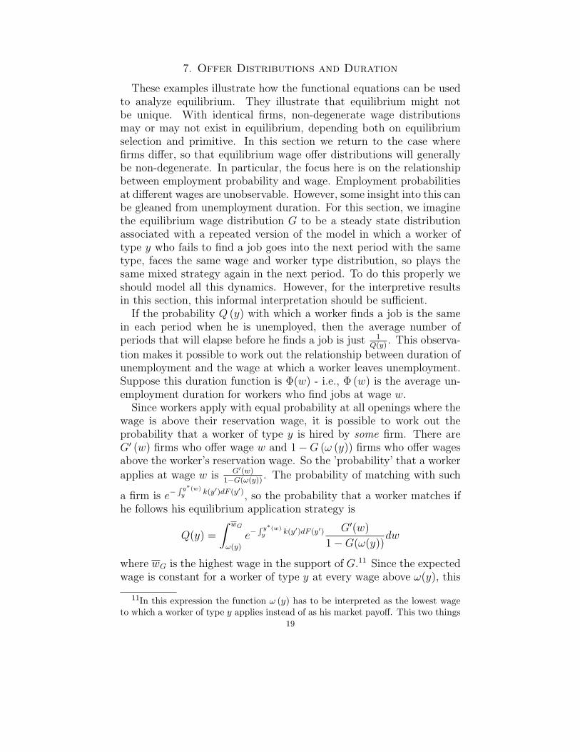
Since workers apply with equal probability at all openings where thewage is above their reservation wage, it is possible to work out theprobability that a worker of type y is hired by some firm. There areG′ (w) firms who offer wage w and 1 − G (ω (y)) firms who offer wagesabove the worker’s reservation wage. So the ’probability’ that a worker

applies at wage w is G′(w)1−G(ω(y))

. The probability of matching with such

a firm is e−R y∗(w)

y k(y′)dF (y′), so the probability that a worker matches ifhe follows his equilibrium application strategy is

Q(y) =

∫ wG

ω(y)

e−R y∗(w)

y k(y′)dF (y′) G′(w)

1 − G(ω(y))dw

where wG is the highest wage in the support of G.11 Since the expectedwage is constant for a worker of type y at every wage above ω(y), this

11In this expression the function ω (y) has to be interpreted as the lowest wageto which a worker of type y applies instead of as his market payoff. This two things

19

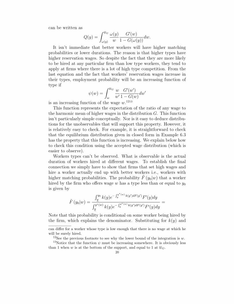
can be written as

Q(y) =

∫ wG

ω(y)

ω(y)

w

G′(w)

1 − G(ω(y))dw.

It isn’t immediate that better workers will have higher matchingprobabilities or lower durations. The reason is that higher types havehigher reservation wages. So despite the fact that they are more likelyto be hired at any particular firm than low type workers, they tend toapply at firms where there is a lot of high type competition. From thelast equation and the fact that workers’ reservation wages increase intheir types, employment probability will be an increasing function oftype if

ψ(w) =

∫ wG

w

w

w′

G′(w′)

1 − G(w)dw′

is an increasing function of the wage w.1213

This function represents the expectation of the ratio of any wage tothe harmonic mean of higher wages in the distribution G. This functionisn’t particularly simple conceptually. Nor is it easy to deduce distribu-tions for the unobservables that will support this property. However, itis relatively easy to check. For example, it is straightforward to checkthat the equilibrium distribution given in closed form in Example 6.3has the property that this function is increasing. We explain below howto check this condition using the accepted wage distribution (which iseasier to observe).

Workers types can’t be observed. What is observable is the actualduration of workers hired at different wages. To establish the finalconnection we simply have to show that firms that set high wages andhire a worker actually end up with better workers i.e., workers withhigher matching probabilities. The probability F (y0|w) that a workerhired by the firm who offers wage w has a type less than or equal to y0

is given by

F (y0|w) =

∫ y0

yk(y)e−

R y∗(w)y k(y′)dF (y′)F ′(y)dy

∫ y∗(w)

yk(y)e−

R y∗(w)y k(y′)dF (y′)F ′(y)dy

=

Note that this probability is conditional on some worker being hired bythe firm, which explains the denominator. Substituting for k(y) and

can differ for a worker whose type is low enough that there is no wage at which hewill be surely hired.

12See the previous footnote to see why the lower bound of the integration is w.13Notice that the function ψ must be increasing somewhere. It is obviously less

than 1 when w is at the bottom of the support, and equal to 1 at wG.20

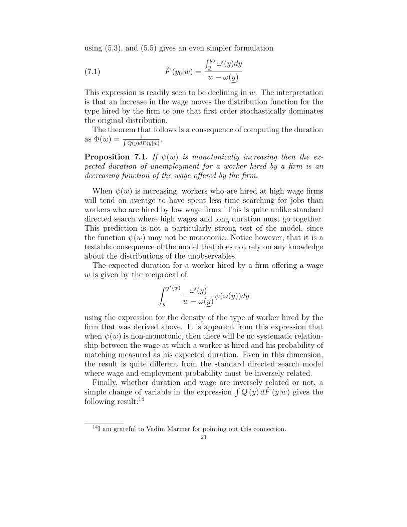
using (5.3), and (5.5) gives an even simpler formulation

(7.1) F (y0|w) =

∫ y0

yω′(y)dy

w − ω(y)

This expression is readily seen to be declining in w. The interpretationis that an increase in the wage moves the distribution function for thetype hired by the firm to one that first order stochastically dominatesthe original distribution.

The theorem that follows is a consequence of computing the durationas Φ(w) = 1

R

Q(y)dF (y|w).

Proposition 7.1. If ψ(w) is monotonically increasing then the ex-pected duration of unemployment for a worker hired by a firm is andecreasing function of the wage offered by the firm.

When ψ(w) is increasing, workers who are hired at high wage firmswill tend on average to have spent less time searching for jobs thanworkers who are hired by low wage firms. This is quite unlike standarddirected search where high wages and long duration must go together.This prediction is not a particularly strong test of the model, sincethe function ψ(w) may not be monotonic. Notice however, that it is atestable consequence of the model that does not rely on any knowledgeabout the distributions of the unobservables.

The expected duration for a worker hired by a firm offering a wagew is given by the reciprocal of

∫ y∗(w)

y

ω′(y)

w − ω(y)ψ(ω(y))dy

using the expression for the density of the type of worker hired by thefirm that was derived above. It is apparent from this expression thatwhen ψ(w) is non-monotonic, then there will be no systematic relation-ship between the wage at which a worker is hired and his probability ofmatching measured as his expected duration. Even in this dimension,the result is quite different from the standard directed search modelwhere wage and employment probability must be inversely related.

Finally, whether duration and wage are inversely related or not, asimple change of variable in the expression

∫

Q (y) dF (y|w) gives thefollowing result:14

14I am grateful to Vadim Marmer for pointing out this connection.21

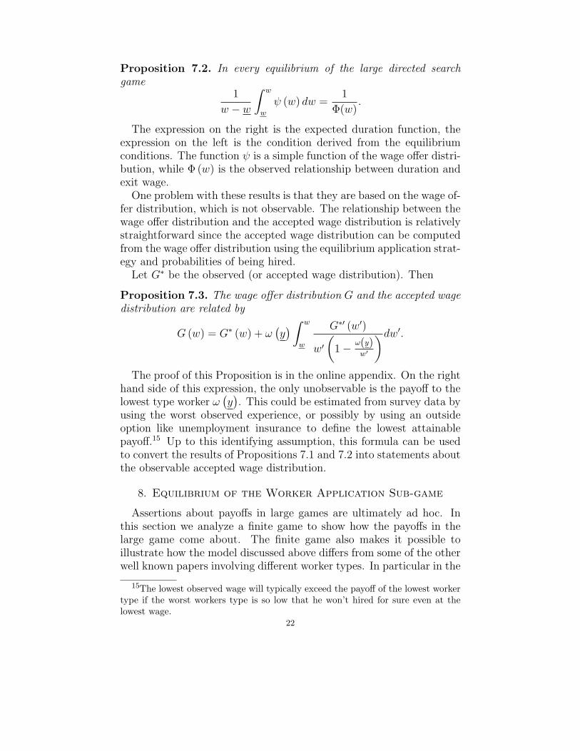
Proposition 7.2. In every equilibrium of the large directed searchgame

1

w − w

∫ w

w

ψ (w) dw =1

Φ(w).

The expression on the right is the expected duration function, theexpression on the left is the condition derived from the equilibriumconditions. The function ψ is a simple function of the wage offer distri-bution, while Φ (w) is the observed relationship between duration andexit wage.

One problem with these results is that they are based on the wage of-fer distribution, which is not observable. The relationship between thewage offer distribution and the accepted wage distribution is relativelystraightforward since the accepted wage distribution can be computedfrom the wage offer distribution using the equilibrium application strat-egy and probabilities of being hired.

Let G∗ be the observed (or accepted wage distribution). Then

Proposition 7.3. The wage offer distribution G and the accepted wagedistribution are related by

G (w) = G∗ (w) + ω(

y)

∫ w

w

G∗′ (w′)

w′

(

1 −ω(y)w′

)dw′.

The proof of this Proposition is in the online appendix. On the righthand side of this expression, the only unobservable is the payoff to thelowest type worker ω

(

y)

. This could be estimated from survey data byusing the worst observed experience, or possibly by using an outsideoption like unemployment insurance to define the lowest attainablepayoff.15 Up to this identifying assumption, this formula can be usedto convert the results of Propositions 7.1 and 7.2 into statements aboutthe observable accepted wage distribution.

8. Equilibrium of the Worker Application Sub-game

Assertions about payoffs in large games are ultimately ad hoc. Inthis section we analyze a finite game to show how the payoffs in thelarge game come about. The finite game also makes it possible toillustrate how the model discussed above differs from some of the otherwell known papers involving different worker types. In particular in the

15The lowest observed wage will typically exceed the payoff of the lowest workertype if the worst workers type is so low that he won’t hired for sure even at thelowest wage.

22

finite model it is easy to see how workers mixed application strategiesdiffer from the mixing that occurs in models like (Shimer 2005) and (Shi2002) where wages can be conditioned on worker type. Furthermore thedistinction between two type models like (Lang, Manove, and Dickens1999) and continuous type models can be made clear. Finally, the finitetype model illustrates why assortative matching of the sort that occursin (Eeckhout and Kircher 2008) cannot occur here.

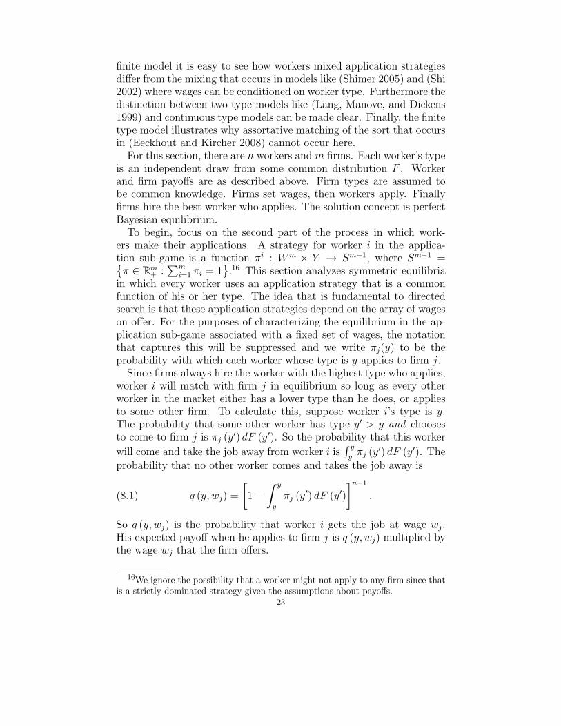
For this section, there are n workers and m firms. Each worker’s typeis an independent draw from some common distribution F . Workerand firm payoffs are as described above. Firm types are assumed tobe common knowledge. Firms set wages, then workers apply. Finallyfirms hire the best worker who applies. The solution concept is perfectBayesian equilibrium.

To begin, focus on the second part of the process in which work-ers make their applications. A strategy for worker i in the applica-tion sub-game is a function πi : Wm × Y → Sm−1, where Sm−1 ={

π ∈ Rm+ :

∑mi=1 πi = 1

}

.16 This section analyzes symmetric equilibriain which every worker uses an application strategy that is a commonfunction of his or her type. The idea that is fundamental to directedsearch is that these application strategies depend on the array of wageson offer. For the purposes of characterizing the equilibrium in the ap-plication sub-game associated with a fixed set of wages, the notationthat captures this will be suppressed and we write πj(y) to be theprobability with which each worker whose type is y applies to firm j.

Since firms always hire the worker with the highest type who applies,worker i will match with firm j in equilibrium so long as every otherworker in the market either has a lower type than he does, or appliesto some other firm. To calculate this, suppose worker i’s type is y.The probability that some other worker has type y′ > y and choosesto come to firm j is πj (y′) dF (y′). So the probability that this worker

will come and take the job away from worker i is∫ y

yπj (y′) dF (y′). The

probability that no other worker comes and takes the job away is

(8.1) q (y, wj) =

[

1 −

∫ y

y

πj (y′) dF (y′)

]n−1

.

So q (y, wj) is the probability that worker i gets the job at wage wj.His expected payoff when he applies to firm j is q (y, wj) multiplied bythe wage wj that the firm offers.

16We ignore the possibility that a worker might not apply to any firm since thatis a strictly dominated strategy given the assumptions about payoffs.

23

This logic can also be used to derive the firm’s profit function. Thefirm hires the best type who applies. So the firm’s expected profitsare determined by the probability distribution of the highest type whoapplies. Fix a type y. The probability that any particular worker eitherhas a type below y or applies at some other firm, using the logic above,

is 1−∫ y

yπj (y′) dF (y′). The probability that all the workers either have

types below y or apply to another firm is[

1 −

∫ y

y

πj (y′) dF (y′)

]n

.

To say this a different way, this is the probability that the highesttype who applies to firm j is less than or equal to y. The probabilitydistribution function has a density given by nq (y, wj) πj (y) F ′ (y). In-tegrating over possible values for this highest type gives the expectedpayoff function for firm j as

ρ (wj, x) =

∫ y

y

v(wj, y, x)nq (y, wj) πj (y) dF (y) .

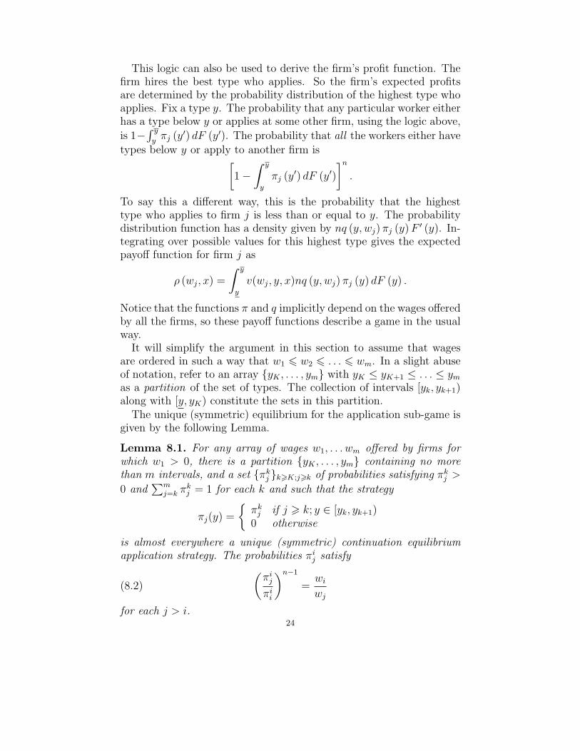
Notice that the functions π and q implicitly depend on the wages offeredby all the firms, so these payoff functions describe a game in the usualway.

It will simplify the argument in this section to assume that wagesare ordered in such a way that w1 6 w2 6 . . . 6 wm. In a slight abuseof notation, refer to an array {yK , . . . , ym} with yK ≤ yK+1 ≤ . . . ≤ ym

as a partition of the set of types. The collection of intervals [yk, yk+1)along with [y, yK) constitute the sets in this partition.

The unique (symmetric) equilibrium for the application sub-game isgiven by the following Lemma.

Lemma 8.1. For any array of wages w1, . . . wm offered by firms forwhich w1 > 0, there is a partition {yK , . . . , ym} containing no morethan m intervals, and a set {πk

j }k>K;j>k of probabilities satisfying πkj >

0 and∑m

j=k πkj = 1 for each k and such that the strategy

πj(y) =

{

πkj if j > k; y ∈ [yk, yk+1)

0 otherwise

is almost everywhere a unique (symmetric) continuation equilibriumapplication strategy. The probabilities πi

j satisfy

(8.2)

(

πij

πii

)n−1

=wi

wj

for each j > i.24

Furthermore, the numbers {yk} and {πkj } depend continuously on the

wages offered by firms.

There are many indices to keep track of, but the logic is simpleenough. Suppose there are only two firms offering wages w1 < w2. Thehighest worker types apply only to firm 2. If y is close enough to y,then even if the other worker is expected to apply at wage w2 for sure,the first worker will get the job with probability F (y). If F (y) w2 > w1

then there is no point applying at wage w1. This immediately describesthe cutoff point ym = y2 to be the point where F (y2) w2 = w1. Thisgives the constant π2

2 = 1.The main content of the theorem comes in the description of what

happens to the types below y2. The theorem says that all types belowy2 use exactly the same application probabilities π1

1 and π12 which are

readily derived from the conditions

π12 =

w1

w2

π11

and the fact that π11 and π1

2 must sum to zero (π12 = w1

w1+w2). The two

application strategies are then

π1 (y) =

{

w2

w1+w2y < y2,

0 otherwise;

and

π2 (y) =

{

w1

w1+w2y < y2

1 otherwise.

The complete proof is included in the appendix. The theorem is hardto state because each worker type has to assign a different probabilityof applying to every different wage. The Lemma shows that Bayesianequilibrium puts three kinds of structure on these strategies. First,it says that if a worker sends an application with positive probabilityto a firm offering a wage wk, then he or she must send applicationsto every higher wage as well. This is the ’reservation wage’ part ofthe story, since the worker has to decide what is the lowest wage towhich he will send an application. Second, the formula (8.2) alongwith the requirement that the application probabilities sum to one,then determines the entire application strategy from the reservationwage. Third, and critically important for most of the technical resultsin the paper, the Lemma partitions the worker type space into intervals,then says that all workers whose type is in the same interval will useexactly the same application probabilities.

25

To see why mixing has to occur, start with the elite types in theinterval [ym, y]. As in the two firm example described above, theyapply only to the highest wage firm. They might as well, since theirtypes are so high they are very likely to be hired at every wage nomatter what the other workers do. The ’marginal’ worker type in thiselite group has type ym. He is just indifferent between applying at thehighest wage firm and getting the job if it happens to be the case thatthere are no other elite workers, and applying at the second highestwage and getting that job for sure.

Now consider a worker whose type is just slightly below ym. If theonly workers who apply to the highest wage firm are workers in the elitegroup, then this infra marginal type has the same chance of finding ajob with the highest wage firm as does the worker of type ym - hewill get the job if none of the other workers has an elite type. Yet ifhe applies at the second highest wage, there is always a chance thathe will lose out to a worker whose type is in between his type andym. Since the worker of type ym is indifferent between the highestand second highest wage, the worker with the lower type must strictlyprefer to apply at the highest wage. So to support an equilibrium,these infra marginal workers whose types are slightly below ym mustface the same competition from other infra marginal workers at thehighest wage firm as they do at the second highest wage firm. In otherwords, infra marginal workers must apply with positive probability atthe highest wage firm. Exactly this same logic extends down throughall the lower types.

This explains the difference between models with a continuum oftypes and models like (Lang, Manove, and Dickens 1999) where thereare only two types.17 As explained above, it is the infra marginalworkers who break up any potential equilibrium where workers sort bytype. When there are only two types, as there are in (Lang, Manove,and Dickens 1999), there are no infra marginal types, so complete sort-ing can be supported when the lower type is just indifferent betweenapplying at the low wage and the high wage. The addition of a thirdworker type in their model without a corresponding firm type to hireit, would lead to an equilibrium in the application subgame that moreclosely resembles the equilibrium described here.

The uniqueness of the mixed equilibrium also explains why assorta-tive matching cannot be supported in equilibrium, as it is in (Eeckhoutand Kircher 2008). The difference between the two models is that

17Two types is a very natural assumption for their problem.26

(Eeckhout and Kircher 2008) assume that the ’proposer’ (or wage set-ter here) doesn’t care directly about the types of the parties involvedin a transaction. This same property could be accomplished here bychanging the offer that the firm makes from a wage to a demand forprofit - i.e., whoever it hires the firm requires the same profit. The firmno longer cares which worker it hires, and workers will naturally matchassortatively (under the payoff restrictions that they provide). Theirapproach is similar to the (Shimer 2005)-(Shi 2002) approach whichmakes the wage contingent on worker type. Yet feasible contracts in(Eeckhout and Kircher 2008) are more restricted than in (Shimer 2005)-(Shi 2002) since firms cannot vary wages arbitrarily across types.

Models like (Shimer 2005) or (Shi 2002) where firm can conditionwages on type also support mixed application strategies, but for a verydifferent reasons. As in (Shi 2002) suppose there are only two typesof firms and two types of workers. High type firms offer high wages toattract high type workers. However, by the nature of directed search,there is a chance they will nonetheless end up without applications.Firms can raise their profits by setting a higher wage in order to attractlower quality applicants, who they will only hire in the event that nohigh quality applicants apply. The higher wage for lower quality isneeded to compensate the low quality workers for the low chance theywill be hired. So mixing among firms of different wages is used tosupport the equilibrium in the wage setting part of the game.

9. Limit Payoffs

Finally, we show the sense in which the large game payoffs we de-scribed in the continuum model in the first part of the paper are limitsof payoffs in finite games. There are a couple of reasons for doing this.First, the matching probabilities and payoff functions used in the con-tinuum model are subtly different than those used in the conventionaldirected search literature. For instance, matching probabilities aren’tbased on the queue size at the firm in the usual way. Furthermore, pay-offs associated with wage offers that exceed all wages in the supportof the existing distribution of wages involve outcomes in which firmssometimes choose the best applicant, and sometimes select randomlyfrom a group of highest quality applicants. Whether or not these func-tions seem plausible descriptions of payoff, they are essentially ad hoc.The limit theorem provided here justifies these payoff functions.

Furthermore, the symmetric continuation equilibrium in worker ap-plications strategies is unique, this limit theorem shows not only thatthe heuristic descriptions of payoffs given in the continuum model are

27

reasonable approximations to payoffs in large finite games, it also showsthat these payoff functions are the only ones that can be used to ap-proximate payoffs in large finite versions of the game.

Lastly, the limit results are designed to provide payoffs for all distri-butions of wages, not just those associated with equilibrium. So theydo not directly address sequences of equilibrium in the wage settingpart of the game. However, it is straightforward to use these results toshow that every sequence of pure strategy equilibrium in finite versionsof the game converges to an equilibrium in the continuum game as wehave described it above. All this requires is a restriction on firms’ pay-off functions that ensure that they don’t vary in ’unreasonable’ wayswith worker types.18 The proof is by contradiction. If convergencefails, then the limit distribution of wages will have the property thata measurable set of firms will want to deviate. Then, provided payoffsaren’t too sensitive to type and wage distributions, then firms will wantto deviate in large finite versions of the game as well. The details ofthis straightforward but lengthy argument are left out in the interestof brevity.

The theorem:

Theorem 9.1. Let G be a distribution of wages, w a wage in the sup-port of G offered by a firm of type x. Let Gn be a sequence of distribu-tions with finite support that converges weakly to G. Then worker andfirm payoffs in the continuation equilibrium in which other firms offerwages given by the mass points in Gn converge to the payoff functionsgiven by (4.1), (4.2), (4.3) and (4.4) given in Section 3 .

The complete proof of this theorem is in the on-line appendix.

10. Conclusion

This paper illustrates how a directed search model can be used tomodel wage competition among firms who can’t condition wage pay-ments on worker type. Part of this involves adjusting the directedsearch model to allow for rich variation in the types of workers andfirms. This improves on existing models that use extensive symmetryassumptions that sometimes force the models to behave in counter-factual ways. In the variant proposed here, rich distributions of firmand worker characteristics can be incorporated.

The directed search model does impose some structure on the data.Surprisingly it restricts the relationship between the wage distribution

18For example, if the family of payoff functions for a firm determined by the setof worker types is equi-continuous.

28

and the function relating unemployment duration and exit wage. Somewage distributions (the uniform being an example) have the propertythat workers who leave unemployment at high wages must also haveshorter unemployment duration. This prediction is distinctly differentfrom standard directed search models where unemployment durationand wage must be positively related.

The driving force in the model presented here is the equilibrium ofthe workers’ application sub-game. Contrary to what one might expect,low quality workers do not restrict their applications to low wage firms.On the contrary, low quality workers make applications at all kinds ofdifferent wages. The higher the unobservable quality of the worker, themore discriminating the worker is in the wages at which he applies.It is this property that breaks the strong relationship between wageand unemployment probability. Higher quality workers are more likely,everything else constant, to be hired by firms. High quality workers alsoapply to higher wage firms on average. In this sense high wages andshort duration should be related. This relationship is not unambiguoushowever. As a workers quality rises, he is more likely to be hired atany given firm, but he will also restrict his applications to firms whosewages are higher. This by itself reduces the probability of employmentbecause high wage firms have bigger queues - the usual directed searchstory.

Finally, the paper suggests how observable data on wages and dura-tion can be used to provide a testable implication of the model.

References

Acemoglu, D., and R. Shimer (2000): “Wage and Technology Dispersion,”Review of Economic Studies, 67(4), 585–607.

Addison, J. T., M. Centeno, and P. Portugal (2004): “Reservation Wages,Search Duration and Accepted Wages in Europe,” IZA DP #1252.

Albrecht, J., P. A. Gautier, and S. Vroman (2006): “Equilibrium DirectedSearch with Multiple Applications,” Review of Economic Studies, 73(4), 869–891.

Delacroix, A., and S. Shi (2006): “Directed Search on the Job and the WageLadder,” International Economic Review, 47, 651–699.

Eeckhout, J., and P. Kircher (2008): “Sorting and Decentralized Price Com-petion,” Working paper, University of Pennsylvania.

Galenianos, M., and P. Kircher (2005): “Directed Search with Multiple Ap-plications,” Working paper, University of Pennsylvania.

Lang, K., and M. Manove (2003): “Wage announcements with a continuum ofworker types,” Annales d’Economie et de Statistique, (71-72), 10.

Lang, K., M. Manove, and W. Dickens (1999): “Racial Discrimination inLabour Markets with Announced Wages,” Boston University working paper.

Mas-Colell, A. (1975): “A Model of Equilibrium with Differentiated Commodi-ties,” Journal of Mathematical Economics, 2(2), 263–295.

29

Mas-Colell, A. (2002): Non-Cooperative Games with Many PlayersElsevier.Peters, M. (2000): “Limits of Exact Equilibria for Capacity Constrained Sellerswith Costly Search,” Journal of Economic Theory, 95(2), 139–168.

Schmeidler, D. (1973): “Equilibrium Points of Nonatomic Games,” Journal of

Statistical Physics, 4, 295–300.Shi, S. (2002): “A Directed Search Model of Inequality with Heterogeneous Skillsand Skill-Based Technology,” Review of Economic Studies, 69, 467–491.

(2009): “Directed Search for Equilibrium Wage Tenure Contracts,”Econo-

metrica, 77, 561–584.Shimer, R. (2005): “The Assignment of Workers to Jobs in an Economy withCoordination Frictions,” Journal of Political Economy, 113, 996–1025.

30