NON-PRICE EQUILIBRIA FOR NON-MARKETED GOODS*

by

Daniel J. Phaneuf, Jared C. Carbone, and Joseph A. Herriges

Commissioned for: Resources for the Future Frontiers of Environmental Economics Workshop,

Washington, DC February 27-28, 2007

Version: June 28, 2007

* The authors are Associate Professor of Agricultural and Resource Economics, North Carolina State University, Assistant Professor of Economics, Williams College, and Professor of Economics, Iowa State University, respectively. We thank without implicating Kerry Smith, Roger von Haefen, Chris Timmins, and several workshop participants for valuable discussions and comments on aspects of this project. Funding for the IA Lakes Project data used in this analysis was provided by the Iowa Department of Natural Resources and the U.S. Environmental Protection Agency's Science to Achieve Results (STAR) program. Although the research described in the article has been funded in part by the U.S. Environmental Protection Agency's STAR program through grant R830818, it has not been subjected to any EPA review and therefore does not necessarily reflect the views of the Agency, and no official endorsement should be inferred Send correspondence to: Prof. Daniel Phaneuf, NCSU Box 8109, Raleigh, NC 277695, (919) 515-4672, dan_phaneuf@ncsu.edu.

Non-Price Equilibria for Non-Marketed Goods

Abstract:

As part of the Resources for the Future Frontiers of Environmental Economics collection of

papers, we consider the problem of general equilibrium feedback effects in non-price space as

they relate to non-market valuation. Our overall objective is to examine the extent to which non-

price equilibria arising from both simple and complex sorting behavior can be empirically

modeled and the resulting differences in partial and general equilibrium welfare measures

quantified. After motivating the problem in general we consider the specific context of

congestion in recreation demand applications, which we classify as the outcome of a simple

sorting equilibrium. Using both econometric and computable general equilibrium (CGE) models

we examine the conceptual and computational challenges associated with this class of problems

and present findings on promising solution avenues. We demonstrate the relevance of accounting

for congestion effects in recreation demand with an application to lake visits in Iowa. Our

econometric and CGE results confirm that, for some plausible counterfactual scenarios,

substantial differences exist between partial and general equilibrium welfare estimates. We

conclude the paper by describing tasks that are needed to move forward research in this area.

JEL Classification: C35, D58, Q25, Q26

1

I. Introduction

Empirical studies of market activities draw on an elegant and coherent body of theory

that describes household and firm interactions in the market place. Price taking households

purchase goods produced by firms that compete to maximize profits under a variety of market

power conditions. Theory provides behavioral predictions for households and firms as well as

statements about how the aggregation of this behavior results in equilibrium price and quantity

outcomes. Models of general equilibrium rely on this link between individual behavior and

aggregate outcomes to describe how exogenous changes lead to both direct and indirect effects in

price and quantity space. Often it is the indirect or feedback, effects, that are the most interesting

in market studies. A variety of empirical and calibration techniques have been developed in

economics to study these effects. The modern empirical IO literature focusing on particular

industries provides a good example of the former while CGE models of whole sectors of the

economy provide good examples of the latter. In both cases the emphasis is on modeling and

understanding equilibrium outcomes in price and quantity space.

The story is quite different in studies of non-market goods that are typically employed by

environmental economists for purposes of non-market valuation. By definition non-marketed

goods are not exchanged in markets, and therefore one cannot speak of equilibrium prices and

quantities for the goods per se. Instead the emphasis is usually on understanding preferences in a

partial equilibrium framework for a quasi-fixed level of a public good. For this purpose an

impressive array of structural econometric models has been developed that are capable of

predicting individuals’ valuations for exogenous changes in the level of the public good. For

example, recreation demand modelers use increasingly sophisticated models of quality

differentiated demands to understand how recreation site attributes affect behavior and well-

being. Hedonic property value models use ever increasing levels of spatially resolute data to

2

parse out the contribution of a local public good to housing prices. Although the latter models

make use of equilibrium concepts to motivate estimation, they rarely are capable of predicting

feedback effects from large-scale changes in public good levels. Thus, with few exceptions, it

seems reasonable to say that non-market valuation has focused primarily on partial equilibrium

analysis of the interactions between behavior and quasi-fixed levels of environmental quality.1

This emphasis is probably reasonable in general. Empirical models of behavior that use

measurable environmental quality as explanatory variables usually find effects that are of second

order importance relative to non-environmental factors. For example, ambient water quality in

recreation demand models is usually much less important in explaining site choice and visitation

frequency than travel cost. Likewise, structural characteristics tend to explain much more of the

variability in housing prices than does air quality in hedonic property value models. Water

quality and air quality in these contexts are examples of non-price attributes that we might

reasonably suppose to be exogenous to the behavior that we are attaching to them. In contrast,

the levels of other types of attributes – such as congestion or angler catch rates in recreation

models, or traffic levels in residential location choice models – are at least partially determined

by the aggregation of behavior under analysis. We may therefore wonder if there are situations in

which general equilibrium feedback effects in endogenous attribute space might be empirically

important in non-market valuation. This might be particularly so for a large-scale policy

intervention that substantially changes the level and spatial distribution of environmental quality.

In this paper we begin to consider the extent to which non-price equilibria and feedback effects

can be identified and accounted for conceptually and in empirical non-market valuation studies.

To examine this question we proceed as follows. We begin by providing a descriptive

overview of how we will think about the concept of ‘non-price equilibria’ in non-market

3

valuation. We suggest working definitions of two general types of non-price equilibria and offer

context and motivation by linking these definitions to specific examples and the existing

literature. We then turn to study a specific type of non-price endogenous attribute: congestion in

recreation demand models. We do this using both econometric and computable general

equilibrium (CGE) models. We begin by laying out a general modeling structure that will be

used in both the econometric and CGE models, which is followed by a description of the Iowa

lakes data that motivates our empirical analysis in both modeling frameworks. We then consider

an empirical model of recreation demand that explicitly includes site congestion as an

explanatory variable, accounts for its econometric endogeneity, and allows computation of both

partial and general equilibrium welfare measures. After presenting results from this analysis we

turn to the CGE model, which is used to explore more generally situations when partial and

general equilibrium welfare measures can be different and under what circumstances it might be

important to consider non-price feedback effects in empirical non-market valuation models.

With the three components of this paper we provide three contributions in the spirit of the

‘frontiers’ theme of this conference. First, we lay out a research agenda that is motivated by the

notion that large scale policy interventions might lead to feedback effects in non-price variables.

Second, we make use of both CGE and econometric modeling approaches to analyze the

feedbacks problem and demonstrate how these quite different tools can shed light on the same

problem from different angles. Since the behavior we are interested in is characterized by both

intensive and extensive margin decisions both modeling approaches must admit binding non-

negativity constraints. Thus a second contribution of this work is the further development of

CGE and econometric models that are flexible, tractable, and provide realistic and internally

consistent representations of the behavior we are modeling. The final contribution involves the

4

application to recreation visits to Iowa lakes and accounting for congestion in the model.

II. Conceptual Overview

To ground our discussion of non-price equilibria we consider the following behavioral

setup. Agents in a closed economy maximize an objective function by choosing levels of

activities that are defined by both price and a set of non-price attributes. In the case of consumers

the activities are demands for quality-differentiated goods; for firms we can think of them as

derived demands for quality-differentiated factor inputs. For the remainder of this discussion we

use terminology corresponding to the consumer’s problem, although we will also provide

examples that correspond to firm’s behavior. Households consume the quality differentiated

goods in non-negative quantities and can, at the optimum, be at a corner solution for a subset of

the available goods. The set of non-price attributes that describe the goods in the choice set can

be divided into two types: those that are exogenously determined and those that are at least

partially determined by the actions of individuals in the model (i.e., endogenous attributes). We

are ultimately interested in understanding the extent to which the levels of endogenous attributes

might change in response to exogenous or policy shocks, and what the resulting differences are

between partial and general equilibrium welfare measures for policy interventions.

This general setup can be better understood by adding a few specific examples. The most

obvious case is when the quality differentiated goods are trips to recreation sites, say a set of

lakes. The demand for trips depends on individual travel costs as well as attributes of the

recreation sites. Attributes such as the presence of boat ramps, picnic facilities, and perhaps

ambient water quality are exogenous to the decision process. In contrast, congestion at the

recreation sites is determined by the aggregate visitation decisions of the people in the economy

and is therefore an endogenous attribute. Similarly, angling catch rates for sport fish species at

the lakes are determined not only by existing bio-physical conditions, but also by the spatial and

5

temporal distribution of anglers’ fishing effort. Policy interventions such as water quality

improvements, facility improvements, or fish stocking programs might have direct welfare

effects as well as indirect effects that play through via the re-equilibrating of congestion and

catch rate attributes that change due to people’s changed visitation patterns.

A second example is the choice of residential location, which conveys a bundle of market

and non-market services. Exogenous attributes in the bundle include characteristics of the

structure and distance to natural features such as lakes. Endogenous attributes might include

traffic congestion and the resulting local air quality impacts, privately held open space, and

publicly held open space created by local governance. This latter attribute is related to other

endogenous attributes that have more of a public finance or urban economic flavor, such as local

school quality and the racial makeup of neighborhoods.

A final example comes from commercial fisheries. Vessel operators choose the timing

and location of harvest effort that gives rise to an aggregate distribution of effort in much the

same way that congestion is determined in a recreation model. This effort, in combination with

the biological system, gives rise to equilibrium populations for the targeted species as well as

equilibrium levels of spatially and temporally distributed catch effort.

These examples suggest two general types of non-price equilibria that can occur in

environmental economics applications. The first case we refer to as a simple sorting equilibrium.

In this case levels of endogenous non-price attributes are determined only by interactions among

agents. Among the examples mentioned this class includes congestion in recreation applications

and more generally social interaction outcomes such as racial mixing and peer effects in schools.

In these cases the equilibrium outcomes are determined only by the interactions among agents.

This is in contrast to the second type of non-price equilibrium that we define which we label a

6

complex sorting equilibrium. This refers to situations in which the agents interact with a quasi-

supplier (often the natural environment) to determine the equilibrium. Among the examples we

have mentioned recreation fishing catch rates fall into this class. Here the natural environment

provides the stock of fish while anglers’ aggregate distribution of trips and catch effort provides

the level of stock exploitation. The interaction results in equilibrium catch rate levels and fish

populations. Educational outcomes in public finance applications are similarly complex sources

of sorting equilibrium. Here the sorting behavior of households into school districts determines

peer effects, while district funding levels determine teacher and facility quality. Together these

factors determine educational outcomes.

To formalize these ideas consider the following model of consumer behavior related to

the choice of quality differentiated goods. There are N consumers in the economy, each of whom

maximizes utility by choosing the levels of a J-dimension vector of quality differentiated goods

denoted by zi and spending on other goods xi. The problem is given analytically by

,

max ( , ; ) . . , 0, 1,..., ,i i

i i i i i i i i ijz xU U z x Q s t p z x y z j J′= + ≤ ≥ = (1)

where Ui is the utility index for person i, Q is an M×J matrix of non-price attributes where M is

the number of attributes, pi is the vector of prices for the quality differentiated goods, and yi

denotes the person’s income. Some or all of the quality attributes in the model may be

endogenously determined by the aggregation of consumers’ behavior and aspects of the natural

environment. Thus we define an attribute transmission function by

1( ,..., ; ), 1,..., , 1,..., ,mj mj Nq q z z E m M j J= = = (2)

where qmj is an individual element of the quality matrix Q, z1,…,zN denotes the aggregate

behavior by households in the economy, and E stands for the natural environment or a quasi-

supplier. The transmission function shown in (2) is general in that it describes an endogenous

7

attribute arising from a complex sorting equilibrium, but it also nests as special cases the two

additional types of attributes we have defined: (a) qmj=qmj(E) for exogenous attributes and

(b) qmj=qmj(z1,…,zN) for endogenous attributes arising from a simple sorting equilibrium.

In making their choices we assume individuals take levels of the attributes as given, so

the first-order conditions for person i are:

( , ; ) / ( , ; ) /

, 0, 0, 1,..., .( , ; ) / ( , ; ) /

i i i ij i i i ijij ij ij ij

i i i i i i i i

U z x Q z U z x Q zp z p z j J

U z x Q x U z x Q x∂ ∂ ∂ ∂⎡ ⎤

≤ − = ≥ =⎢ ⎥∂ ∂ ∂ ∂⎣ ⎦ (3)

Equilibrium in the economy is characterized by the simultaneous solution to a system of

equations and their associated complementary slackness relationships that correspond to:

The first-order conditions described by (3) for all individuals i = 1,…,N and

The attribute transmission functions in (2) for j=1,…,J and ,m M∈ where

{ }1, ,M M⊆ … is the set of endogenous attributes.

In defining non-price equilibria we have thus far tried to be fairly general, but it is clear

that this can only be taken so far. Unlike price and quantity equilibrium concepts for

homogenous goods, for which theory provides quite general results, non-price equilibria for

quality differentiated goods are by definition context specific. The challenge for applied welfare

analysis is to characterize conceptually and empirically the particulars of the equilibrium of

interest. Simple sorting equilibria seem easier to deal with than their complex counterparts in that

for the former the analyst need only specify the mechanism through which agents interact, while

for the latter agent interactions a production function and the relationship between the two must

be spelled out.

III. Literature Review

Concerns about equilibrium concepts defined over non-price attributes are not new to the

8

economics literature, though they have typically taken a back seat to analyses based on price

movements. Often these discussions are cast in the context of spatial sorting. Schelling [26]

provides one of the earlier examples, illustrating qualitatively how non-market adjustments

might lead to surprising equilibrium outcomes in the context of racial segregation. A second

example concerns school quality and the role of peer effects in educational outcomes. These

areas have been the subject of substantial research, and include recent studies that apply concepts

and approaches similar to what we draw upon in this paper. Two examples are [3] and [12].

Bayer and McMillian [3] study the role of racial sorting in determining endogenous

neighborhood quality levels such as average education attainment. Their hypothesis is that

preferences for racial clustering may contribute to lower equilibrium neighborhood amenities for

blacks, particularly for average education levels, since the proportion of college educated blacks

is smaller than for whites. To test this hypothesis they estimate a sorting model of residential

location choice and use the model to conduct counter-factual analysis related to neighborhood

race and average educational level outcomes. They find, for example, that a hypothetical

weakening of preferences among blacks to live in the vicinity of other blacks reduces the racial

gap in neighborhood amenities, implying that racial preferences are nearly as important as

differences in socio-economic status in explaining the observed amenity gaps. For each of their

counterfactual experiments new non-price simple sorting equilibrium outcomes for amenities and

race patterns must be calculated.

Ferreyra [12] examines the general equilibrium impacts of school voucher programs.

Households have preferences for location characteristics and school quality as well as the secular

status of private school options. Private and public school quality are endogenously determined

in equilibrium by the composition of households within a district and a school quality production

9

function that depends on spending per student. In this sense the non-price equilibria considered

by [12] are complex sorting outcomes. Ferreyra considers the impacts different hypothetical

voucher programs. She finds that private school enrollment expands and residential location

choice is affected, suggesting that vouchers break the ‘bundling’ that typically exists in the

purchase of public school quality and residential location. These findings depend critically on the

ability to simulate new equilibrium outcomes using the structure of the estimated model.

Recent papers in empirical industrial organization (e.g., [21,25]) provide additional

examples of explicit attention to sorting equilibrium outcomes, notably in the context of firms’

entry location decisions. Geography is a factor over which firms often seek to differentiate their

products. This is particularly the case for retail operations in which proximity to potential

consumers increases the payoff from entry into a location. Competitive pressure from other

retailers in close proximity, however, decreases the payoff. Thus firms must balance competing

factors in deciding whether or not to place a store in a given location, and must make the

decision based on expectations of what competing firms will decide to do. Thus simple sorting

equilibria arise in these contexts and must be accounted for empirically.

There is also research in the environmental literature that addresses aspects of the non-

price equilibrium concepts we consider in this paper. The most closely related study to ours is

Timmins and Murdock [30], who consider the role of congestion in a site choice model of

recreation demand. Congestion in their model is a (dis)amenity determined endogenously by the

aggregate proportion of people who chose to visit a particular site. [30] considers both partial and

general equilibrium welfare measures for changes in site characteristics and availability, where

the latter takes account of agents’ re-sorting (and hence new congestion levels) in response to

exogenous changes. The authors find substantial differences between the two types of welfare

10

measures, and show that congestion is a major determinant of visitors’ choices. Congestion as

defined in [30] falls under our simple sorting equilibrium category. A second and more complex

consideration of an endogenous amenity is Walsh [33]. Using a residential sorting model [33]

examines the role of public and private open space amenities in which both are endogenously

determined. The author models feedback effects associated with urban land use policies, and

finds several surprising results that arise based on his ability to simulate counterfactual land use

outcomes in response to policy shocks. Most importantly he finds that public open space creation

crowds out private open space in general equilibrium, in some cases so much that the total open

space in an urban area falls following a public initiative.

A second area of environmental economics that is relevant for our study is the recent

work on estimating integrated biological and human systems. For example, [19] examines the

impact of water quality improvements on recreational fishing in Maryland’s costal bays. The

unique feature of their analysis is that, while they consider only exogenous water quality

changes, these changes impact recreational fishing choices indirectly through a bio-economic

model of the coastal fishery. The dynamic evolution of the fish stock is modeled as a function of

water quality, allowing water quality improvements to directly affect fish stocks and indirectly

affect anglers via improved catch rates. Additional examples in bio-economics are provided by

[27,28] in commercial fisheries. These papers are distinguished by linked economic and

biological models in which fish stocks are endogenously determined by the interactions between

fishing behavior and the underlying biology.

Although different in their objectives these examples from the housing demand, public

finance, industrial organization, and environmental literatures share similar challenges. These

challenges can be categorized along three dimensions. The first involves econometrically

11

identifying the effect of an endogenous aggregate outcome in individual behavioral models such

as recreation or residential site choice. Manski [18] provides an intuitive overview of what he

calls the reflection problem in the context of nonmarket interactions, which is particularly

relevant for understanding simple sorting outcomes. He describes the difficulty inherent in

“…inferring the nature of an interaction process from observations on its outcomes (when

outcome data) typically have only limited power to distinguish among alternative plausible

hypotheses” (p. 123). From a practical perspective this involves distinguishing between actual

interactions, correlated unobservables, and non-random treatments across agents. For the case of

congestion in recreation demand models the challenge is to separately assess how aggregate site

visitation patterns reflect both the observed and unobserved site attributes that increase visitation,

and congestion externalities that discourage visitation. The second challenge involves defining

equilibrium concepts and describing their properties. Non-price equilibria will often be based on

contexts that are specific to the problem under study. Transmission functions, equilibrating

forces, and the existence and uniqueness of equilibria need to be separately specified and

examined, and these tasks can present non-trivial difficulties. [6], for example, discusses the

properties of equilibria that arise in discrete choice models with simple sorting outcomes that can

take the form of a congestion or agglomeration effect. While they are able to establish general

existence and bounded uniqueness results it is not immediately clear that these findings extend to

more complicated modeling environments. The third challenge that arises in modeling non-price

equilibrium outcomes is computational. In each of the studies described above the objective is to

assess the effect of a counterfactual change in some exogenous factor. This involves solving the

model to determine a new equilibrium – a task that will usually involve numerical methods

nested in multiple layers of simulation.

12

The new classes of locational equilibrium sorting models represent the major empirical

frameworks for examining non-price equilibria and addressing the three modeling challenges.

Our work in this paper draws heavily on insights from the two major strands of this literature:

vertical and horizontal modeling approaches. The former is based on Epple and Sieg [11], which

has its intellectual roots in the public finance literature focused on understanding how

populations stratify across urban landscapes. In this approach to modeling households agree on a

ranking of choice alternatives – typically neighborhoods – based on price and non-price

attributes. Assumptions on preferences are then used to derive equilibrium conditions that are

assumed to hold for any observed outcome in the data. These conditions are used to recover

estimates of preferences for attributes of the neighborhoods – including, perhaps, endogenous

attributes as in [33]. [29], in contrast, examine the equilibrium effects of an exogenous change in

air quality stemming from reduced ozone levels. Sorting in this case occurs on the basis of

preferences for housing, education and air quality in the LA Air Basin between 1989 and 1991.

The horizontal strand of literature has its intellectual roots in the industrial organization

literature and is based in large part on Berry [7] and Berry et al. [8]. These models take the

familiar discrete choice framework as the basis for demand modeling and exploit a two stage

estimation strategy that allows the use of common IV methods to account for endogenous

choices attributes. [4] describes how these tools can be used in a residential sorting context and

[5] and [30] provide examples in environmental applications. A distinguishing feature of these

models is the emphasis on a single choice outcome, such as choice of a place to live or recreation

site to visit. In our analysis below we use many of the modeling techniques introduced in the

horizontal sorting models, but generalize the analysis to include a broader choice environment

that considers both intensive and extensive margin decisions. We also pursue a Bayesian

13

approach to modeling, examined in the context of industrial organization models by [35].

IV. Modeling Framework

In order to assess the feedback effects we are interested in, the non-price equilibrium

outcomes need to be linked in a consistent manner to estimable models of individual behavior.

The models must be able to capture consumer response to changing price and quality conditions

and allow for those responses to occur at both the intensive and extensive margins. This is

particularly important when evaluating major policy shifts that will induce some individuals to

enter or leave the market entirely (i.e., when corner solutions emerge). What is required is a

model that readily admits the concept of a virtual price. By virtual price we mean a summary

measure that consistently and succinctly captures all constraints on behavior, both price and non-

price, which in turn ultimately determines people’s choices. The KT model [23,32] and its dual

counterpart [17,22,24] are uniquely positioned for this purpose. The latter is particularly

attractive in that it involves a direct parameterization of individuals’ virtual prices.

In this section of the paper we provide a general overview of the dual modeling

framework and a discussion of the particular functional form that will be used in our application

and CGE analysis. A detailed discussion of the estimation procedure is delayed until section VI,

which follows our description of the application in section V.

A. The Dual Model

The dual model begins with the specification of the individual’s underlying indirect

utility function. Dropping the individual subscripts for the moment let H(p,y;Q,θ,ε) denote the

solution to a utility maximization problem defined by:

( ) ( ){ }, ;Q, , ; , , | ' ,z

H p y Max U z Q p z x yθ ε θ ε= + = (4)

where as above (z,x) denotes the private goods to be chosen by the individual, p is the vector of

14

corresponding prices, y denotes income, and Q is a vector or matrix of public goods that the

individual agent takes as given. In our application considering the demand for recreation the

private goods include recreation trips to the available sites and all other spending, p reflects the

costs of traveling to those sites, and Q includes the quality attributes of the sites. These attributes,

while taken as given by the individual, include factors (such as congestion and fish stock) that

are determined in equilibrium by the decisions made in the market as a whole. The direct utility

function U(z;q,θ,ε) depends upon parameters θ and attributes of the individual ε that are

unobserved by the analyst.

It is important to note that the indirect utility function in equation (4) is derived without

imposing non-negativity constraints on demand. Applying Roy’s Identity to equation (4) thus

yields notional (or latent) demand equations

( ) ( )*

1, ; , , , ; , , , 1, , ,

J

j j k kk

z H p y Q p H p y Q j Jθ ε θ ε=

= =∑ … (5)

where ( ) ( ), ; , , , ; , , /j jH p y Q H p y Q pθ ε θ ε≡ ∂ ∂ . Note that ( )* * , ; , ,j jz z p y Q θ ε= will be negative

for goods the individual does not wish to consume and positive for those goods she does

consume. Observed consumption levels are then derived through the use of virtual prices, which

rationalize the observed corner solutions. For example, suppose that the first r goods are not

consumed. Let pN=(p1,…,pr)' denote the prices for the non-consumed (i.e., corner solution) goods

and pC=(p1+r,…,pJ)' denote the prices for the consumed goods (i.e., those with positive

consumption). The virtual prices for the non-consumed goods are implicitly defined by

( ) ( )10 ; , , , , ; , , , , ; , , , 1, , .j C r C CH p Q p Q p y Q j rπ θ ε π θ ε θ ε= =⎡ ⎤⎣ ⎦… … (6)

The observed demands for all the commodities become

15

( ) ( ) ( )* * *

1

0 1, ,, ; , , , ; , , , ; , ,

0 1, , ,

J

j j k k jk

j rz H p y Q p H p y Q z p y Q

j r Mθ ε θ ε θ ε

=

= =⎧= = ⎨> = +⎩

∑……

(7)

where p*=(π1,…,πr, p1+r,…,pJ)'. The virtual prices are similarly linked to observed prices,

( )*1,...,

, ; , ,1, , .

jj

j

p j rp y Q

p j r Mπ θ ε

≤ =⎧⎪⎨= = +⎪⎩ …

(8)

The system of equations in (7) and (8) provides the connections between the observed data on

usage (and prices) and the implied restrictions on the underlying error distributions, which can in

turn be used for estimation. These equations allow us to express the indirect utility function (the

solution to the utility maximization problem with non-negativity constraints enforced) as

( ) { }, ; , , max ( , ; , , ) ,V p y Q H p y Qω

ωθ ε θ ε

∈Ω= (9)

where Ω denotes the set of all possible demand regimes (combinations of corner and interior

solutions among the J sites) and pω denotes the particular combination of virtual and actual

prices associated with demand regime ω. The comparison of true and virtual prices as shown in

equation (8) distinguishes the chosen goods from the non-chosen goods and thus can be used to

gauge movements into and out of the market for particular commodities. In addition the virtual

prices are functionally dependent on both the price and non-price attributes of the goods. Thus it

is appropriate to view the virtual prices as quality-adjusted endogenous reservation prices, which

can change in response to either price or non-price attribute changes.

B. Model Specification

The dual model specification can by obtained by choosing a functional form for the

underlying indirect utility function H(p,y;Q,θ,ε) and deriving from it the corresponding notional

demand and virtual price equations [17]. Alternatively, as in [34], one can begin with a system of

notional demands for the goods of interest (i.e., an incomplete demand system) and integrate

16

back to obtain the underlying quasi-indirect utility function. The advantage of the latter approach

is that tractable notional demand equations can be specified, making the computation of virtual

prices straightforward. The disadvantage here, of course, is that the resulting demand system is

incomplete and does not capture substitution possibilities to goods outside of the choice set. In

addition the restrictions needed to ensure integrability tend to require a choice between

substitution and income effects.

Our empirical specification begins with the system of Marshallian notional demands

*

1

, 1, , ,J

ij j jk ik j i ijk

z p y j Jα β γ ε=

= + + + =∑ … (10)

where the subscript i denotes people i=1,…,N and αj=αj(qj,ξj) is a function of both observable

site attributes for site j (the vector qj – the component of Q specific to site j) and unobservable

factors which we denote ξj. We assume that these factors have a linear form given by

, 1, , .j j jq j Jα γ ξ′= + = … (11)

The remaining notation is as follows: pik is the price of site k for individual i and yi denotes

individual i’s income level. We impose a series of restrictions on the parameters of (10) to make

the system of equations weakly integrable [16]. Specifically, we assume that ,jk kj j kβ β= ∀ and

0j jγ = ∀ . The resulting notional demand system becomes:

*

1

, 1, , .J

ij j jk ik ijk

z p j Jα β ε=

= + + =∑ … (12)

The corresponding (notional) quasi-indirect utility function for (12) is given by:

( ) ( )1 1 1

, ; , ,J J J

i i i i j ij ij jk ij ikj j k

H p y Q y p p pθ ε α ε β= = =

⎡ ⎤= − + +⎢ ⎥

⎣ ⎦∑ ∑∑ . (13)

As indicated above the notional demand equations can be used to define virtual prices for the

17

non-consumed goods that rationalize the observed corner solutions. For illustration, suppose

again that the first r goods are not consumed. The virtual prices for these commodities are then

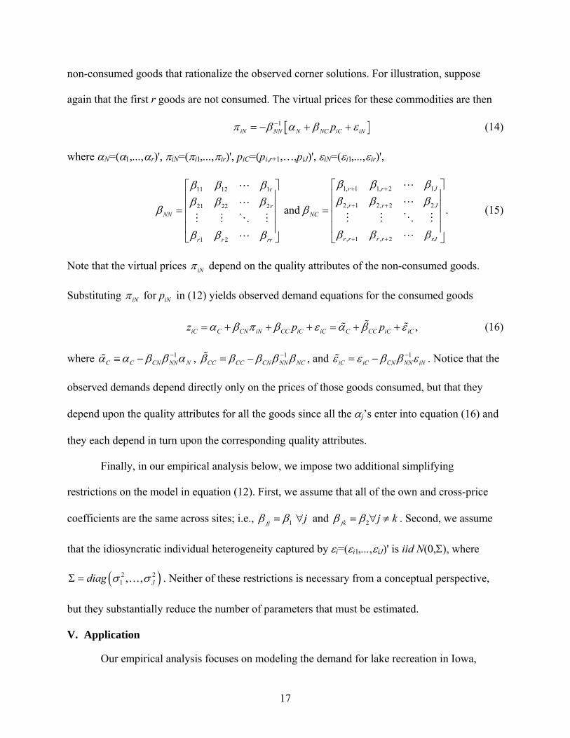
[ ]1iN NN N NC iC iNpπ β α β ε−= − + + (14)

where αN=(α1,...,αr)', πiN=(πi1,...,πir)', piC=(pi,r+1,…,piJ)', εiN=(εi1,...,εir)',

1, 1 1, 2 111 12 1

2, 1 2, 2 221 22 2

, 1 , 21 2

and .

r r Jr

r r JrNN NC

r r r r rJr r rr

β β ββ β ββ β ββ β β

β β

β β ββ β β

+ +

+ +

+ +

⎡ ⎤⎡ ⎤⎢ ⎥⎢ ⎥⎢ ⎥⎢ ⎥= =⎢ ⎥⎢ ⎥⎢ ⎥⎢ ⎥

⎣ ⎦ ⎣ ⎦

(15)

Note that the virtual prices iNπ depend on the quality attributes of the non-consumed goods.

Substituting for iN iNpπ in (12) yields observed demand equations for the consumed goods

,iC C CN iN CC iC iC C CC iC iCz p pα β π β ε α β ε= + + + = + + (16)

where 1C C CN NN Nα α β β α−≡ − , 1

CC CC CN NN NCβ β β β β−= − , and 1iC iC CN NN iNε ε β β ε−= − . Notice that the

observed demands depend directly only on the prices of those goods consumed, but that they

depend upon the quality attributes for all the goods since all the αj’s enter into equation (16) and

they each depend in turn upon the corresponding quality attributes.

Finally, in our empirical analysis below, we impose two additional simplifying

restrictions on the model in equation (12). First, we assume that all of the own and cross-price

coefficients are the same across sites; i.e., 1jj jβ β= ∀ and 2jk j kβ β= ∀ ≠ . Second, we assume

that the idiosyncratic individual heterogeneity captured by εi=(εi1,...,εiJ)' is iid N(0,Σ), where

( )2 21 , , Jdiag σ σΣ = … . Neither of these restrictions is necessary from a conceptual perspective,

but they substantially reduce the number of parameters that must be estimated.

V. Application

Our empirical analysis focuses on modeling the demand for lake recreation in Iowa,

18

drawing on data from the first year of the Iowa Lakes Project (see [2] for an overview). This

project is a four-year panel data study, analyzing the visitation patterns to 129 Iowa lakes by

8000 randomly selected households, providing a rich source of variation in usage patterns. Iowa

is particularly well suited for our research for several reasons. First, Iowa’s lakes are

characterized by a wide range of water quality, including both some of the cleanest and some the

dirtiest lakes in the world. Second, detailed information is available on the environmental

conditions in each lake, including physical and chemical measures (e.g., Secchi transparency,

total nitrogen, etc.) obtained three times each year during the course of the project. Third, Iowa is

currently considering major lake water remediation efforts. These include multi-million dollar

projects to improve target lakes as well as the Governor’s stated objective to remove all of

Iowa’s lakes from the US EPA’s impaired water quality list by 2010. These changes provide

natural, and policy relevant, sets of scenarios to consider in investigating the general equilibrium

effects of regulatory interventions.

The 2002 Iowa Lakes Project survey was administered by mail to a randomly selected

sample of 8000 households. A total of 4423 surveys were completed, for a 62% response rate

once non-deliverables surveys are accounted for. The key section of the survey for the current

analysis obtained information regarding the respondents’ visits to each of 129 lakes during 2002.

On average, approximately 63% of Iowa households were found to visit at least one of these

lakes in 2002, with the average number of day trips per household per year being 8.1. There are,

of course, a large number of corner solutions in this dataset, with 37% of the households visiting

none of the lake sites and most households choosing only a small subset of the available sites.

Fewer than 10% of those surveyed visited more than five distinct sites during the course of a

year. For the purposes of the econometric analysis below, a sub-sample of the 2002 usage data

19

was used. Specifically, we had available 1286 observations, randomly selected from the full

sample. These records were further narrowed to the 749 users in the sub-sample (i.e., households

taking at least one trip in 2002).

The Iowa Lakes survey data was supplemented with two data sources. First, for each

individual in the sample, travel distance and time from their home to each of 129 lakes were

calculated using the transportation software package PCMiler. Travel costs were then computed

using a distance cost of $0.28/mile and valuing the travel time at one-third the individual’s wage

rate. The average travel cost over all site/individual combinations was $135. Second, water

quality measures for each of the lakes were provided by the Iowa State Limnological Laboratory.

The average Secchi transparency and Chlorophyll levels are used in the current analysis. Secchi

transparency measures water clarity and ranges from 0.09 to 5.67 meters across the 129 lakes in

our sample. Chlorophyll is an indicator of phytoplankton plant biomass which leads to greenness

in the water, and ranges from 2 to 183 μg/liter among the Iowa lakes.

VI. Estimation Algorithm

The estimation of the parameters in our model of recreation demand can be divided into

two stages. In the first stage, we estimate the basic parameters in the demand system

characterized by equations (7) and (8). Specifically, we obtain posterior distributions for the

2J+2 parameters θ=(α1,...,αJ, β1, β2, σ1,...,σJ) using a Bayesian computational approach relying

on Gibbs sampling and data augmentation. Note that site specific intercept terms capture all of

the site specific attributes, including the endogenous factors of interest and unobserved site

characteristics. The purpose of the second stage then is to estimate the functional relationship

between these intercepts and the observed quality attributes.

A. First Stage Estimation

Data augmentation techniques pioneered by [1] in the context of discrete choice models

20

provide a powerful tool for handling latent variables, simulating these missing components of the

data and, in doing so, making the analysis more tractable. In the current context, the latent

variables are the notional demands. Together with Gibbs sampling techniques we can use data

augmentation to simulate values from the posterior distribution of interest.2

Formally, the posterior distribution is characterized by

( ) ( ) ( ) ( )* * *, | | , |p z z p z z p z pθ θ θ θ∝ . (17)

Note that the data augmentation procedure treats the unknown latent factors essentially as

additional parameters, characterized in terms of a prior distribution and for which a posterior

distribution is generated. The priors for θ are assumed to take the following forms:

( )~ , mN Iα

ψ ψ τβ

⎛ ⎞≡ ⎜ ⎟

⎝ ⎠, (18)

where τ is a large constant and Im is an m×m identity matrix with m=J+2, and the 2jσ are

independent inverted gamma variates with ( )2 ~ 1,j jIG sσ . While the joint posterior distribution

in (17) is complex, the corresponding conditional posterior distributions for z*, ψ, and 2jσ each

have convenient functional forms. Details of the iterative Gibbs sampling routine used to

simulate draws from the posterior distribution are provided in Appendix A to this paper.

B. Second Stage Estimation

The first stage provides realizations from the posterior distribution for the parameters

α1,…,αJ as well as the price and error variance terms. In this subsection we are interested in

decomposing the intercepts into components that represent the observable and unobservable

attributes of the recreation sites. Since the former will include endogenous attributes that

ultimately drive the general equilibrium aspects of the model this decomposition is important.

Likewise any welfare analysis concerning site attributes (partial or general equilibrium) will

21

require understanding how demand is impacted by changes in observable site quality levels.

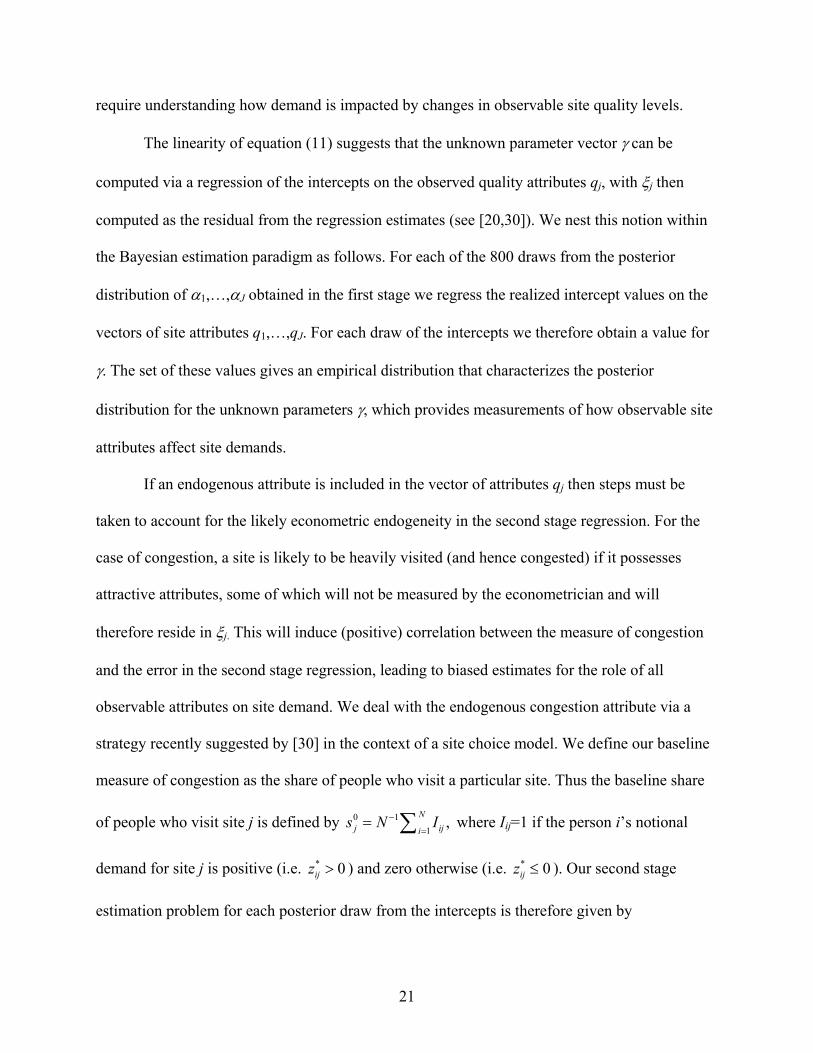
The linearity of equation (11) suggests that the unknown parameter vector γ can be

computed via a regression of the intercepts on the observed quality attributes qj, with ξj then

computed as the residual from the regression estimates (see [20,30]). We nest this notion within

the Bayesian estimation paradigm as follows. For each of the 800 draws from the posterior

distribution of α1,…,αJ obtained in the first stage we regress the realized intercept values on the

vectors of site attributes q1,…,qJ. For each draw of the intercepts we therefore obtain a value for

γ. The set of these values gives an empirical distribution that characterizes the posterior

distribution for the unknown parameters γ, which provides measurements of how observable site

attributes affect site demands.

If an endogenous attribute is included in the vector of attributes qj then steps must be

taken to account for the likely econometric endogeneity in the second stage regression. For the

case of congestion, a site is likely to be heavily visited (and hence congested) if it possesses

attractive attributes, some of which will not be measured by the econometrician and will

therefore reside in ξj. This will induce (positive) correlation between the measure of congestion

and the error in the second stage regression, leading to biased estimates for the role of all

observable attributes on site demand. We deal with the endogenous congestion attribute via a

strategy recently suggested by [30] in the context of a site choice model. We define our baseline

measure of congestion as the share of people who visit a particular site. Thus the baseline share

of people who visit site j is defined by 0 11

,Nj iji

s N I−=

= ∑ where Iij=1 if the person i’s notional

demand for site j is positive (i.e. * 0ijz > ) and zero otherwise (i.e. * 0ijz ≤ ). Our second stage

estimation problem for each posterior draw from the intercepts is therefore given by

22

00 , 1,..., ,j c jc s j j

c

q s j Jα γ γ γ ξ= + + + =∑ (19)

and an instrumental variable is needed for 0js . Appendix A provides additional details on how we

construct an instrument and complete the second stage analysis.

C. Welfare Analysis

In this section we describe how welfare analysis of changes in prices or attributes at the

recreation sites proceeds. As discussed in [23,31,32], welfare analysis in this class of models is

complicated by many factors, including the need to simulate behavior under counterfactual

conditions. The steps needed for analysis using the dual model are particularly challenging and

involve subtle technicalities and many computational issues that at this stage of research are not

fully understood. The added complexity of computing general equilibrium welfare measures

compounds the difficulties. Thus we focus in this section on laying out the broad steps needed

for computing welfare measures, forgoing many of the technical details in favor of a discussion

of the conceptual challenges that we have solved and those that must still be examined.

The first and second stages of the estimation algorithm provide summaries via posterior

means of the utility function parameters and the error variances that constitute the unknowns in

the model. From these summaries preferences are characterized up to the values of the

idiosyncratic errors (i.e., the εij’s). Because the idiosyncratic errors are given a structural

interpretation the utility function is random from analyst’s perspective, which implies that the

compensating surplus for changes in prices or site attributes will also be random variables. Thus

the objective of welfare analysis is to estimate the expected value of an individual’s

compensating surplus by integrating out the unobserved determinants of choice. This requires

that we simulate values of the idiosyncratic errors for each person many times and compute the

welfare measure of interest for each simulated draw. Averaging over the welfare measures for

23

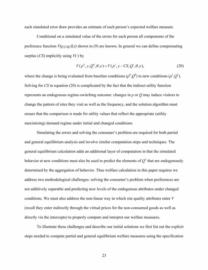
each simulated error draw provides an estimate of each person’s expected welfare measure.

Conditional on a simulated value of the errors for each person all components of the

preference function V(p,y;q,θ,ε) shown in (9) are known. In general we can define compensating

surplus (CS) implicitly using V(·) by

0 0 1 1( , , , , ) ( , , , , ),V p y Q V p y CS Qθ ε θ ε= − (20)

where the change is being evaluated from baseline conditions (p0,Q0) to new conditions (p1,Q1).

Solving for CS in equation (20) is complicated by the fact that the indirect utility function

represents an endogenous regime-switching outcome: changes in p or Q may induce visitors to

change the pattern of sites they visit as well as the frequency, and the solution algorithm must

ensure that the comparison is made for utility values that reflect the appropriate (utility

maximizing) demand regime under initial and changed conditions.

Simulating the errors and solving the consumer’s problem are required for both partial

and general equilibrium analysis and involve similar computation steps and techniques. The

general equilibrium calculation adds an additional layer of computation in that the simulated

behavior at new conditions must also be used to predict the elements of Q1 that are endogenously

determined by the aggregation of behavior. Thus welfare calculation in this paper requires we

address two methodological challenges: solving the consumer’s problem when preferences are

not additively separable and predicting new levels of the endogenous attributes under changed

conditions. We must also address the non-linear way in which site quality attributes enter V

(recall they enter indirectly through the virtual prices for the non-consumed goods as well as

directly via the intercepts) to properly compute and interpret our welfare measures.

To illustrate these challenges and describe our initial solutions we first list out the explicit

steps needed to compute partial and general equilibrium welfare measures using the specification

24

we are working with. We then describe the steps in more detail. Given the posterior means for

the utility and error distribution parameters partial equilibrium welfare analysis for a single

person i and a single draw of the errors involves the following steps:

1) Draw values of the errors εi1,…,εiJ from the estimated distribution for the unobserved

component of utility conditionally such that observed levels of demand at baseline

conditions are replicated for person i. That is, draw errors such that

0 0 0 0 ,iC C NC iN CC C iCz pα β π β ε= + + + (21)

where the notation follows from equation (16), superscripts ‘0’ indicate that all price

and quality variables are set to their baseline values, and 0iCz denotes the observed

level of visits for person i to the set of visited sites C.

2) Determine the total baseline consumer surplus from the consumed goods by

integrating under the baseline demands in equation (21) between 0iCp and 0ˆ iCp , where

0ˆ iCp is the choke price for the set of goods C at baseline conditions. Because the

ordinary and compensating demand curves are the same in our case this is also the

total Hicksian consumer surplus.

3) Define the counterfactual scenario to consist of new prices and/or exogenous site

attribute levels 1 11,...,i iJp p and 1 1

1 ,..., ,Jα α where

1 1 00 , 1,..., ,j c jc s j j

c

q s j Jα γ γ γ ξ= + + + =∑ (22)

and the 1 'jcq s hold new levels of the exogenous attributes. For a partial equilibrium

analysis the original levels of the endogenous attributes (congestion) are maintained.

4) Determine the new demand regime by computing the new notional demands using

25

*1 1 1

1

, 1,..., ,J

ij j jk ik ijk

z p Jα β ε=

= + +∑ (23)

and observe the pattern of positive and negative values for *1ijz . The combination of

positive and negative values for each site is a candidate 1C for the new demand

regime, which must be evaluated and updated as described below. Via the updating the

new demand regime C1 is determined.

5) Determine the total baseline consumer surplus from the consumed goods at the new

demand regime by integrating under 1 1 1 1 1 1 1 11 1 1 1iC C NC iN C C C iC

z pα β π β ε= + + + between 11iC

p

and 11ˆiC

p , where 11ˆiC

p is the choke price for the set of goods C1 at changed conditions.

6) Compensating surplus for person i for this draw of the error is the difference between

total surplus at initial and changed conditions.

A few comments on this algorithm should be made. First, the algorithm focuses on obtaining

use-only values from changes in the levels of attributes by only including areas under the

demand curves for sites that are actually visited. A utility function approach as shown in general

in equation (20) would also add surplus to the total for sites that were not visited. We have

chosen to focus on use value to aid in interpretation and avoid complexities associated with

general equilibrium feedbacks interacting with non-use value computation. Also, we are

assuming in this algorithm that changes in observable attributes from Q0 to Q1 leave unobserved

attribute levels unchanged. That is, ξj is constant for all sites across all changes. Depending on

the scenario this may or may not be a realistic assumption.

For general equilibrium welfare measurement the same steps are needed, but we must

also update the level of the endogenous attribute. Step 3' for the GE case becomes

3’) Define the counterfactual scenario to consist of new prices and candidate site attribute

26

levels defined by 1 11,...,i iJp p and 1 1

1 ,..., ,Jα α where

1 1 00 , 1,..., ,j c jc s j j

c

q s j Jα γ γ γ ξ= + + + =∑ (24)

and the 1 'jcq s hold new levels of the exogenous attributes. For general equilibrium

measurement an algorithm is needed that updates 1 11 ,..., ,Jα α to 1 1

1 ,..., ,Jα α where

1 1 10 , 1,..., ,j c jc s j j

c

q s j Jα γ γ γ ξ= + + + =∑ (25)

and 1js is the new equilibrium proportion of people who visit site j given the changed

conditions. We discuss the form that this updating takes below.

These six steps each present varying degrees of computational and conceptual challenges.

Step 1 is technical but quite similar to the data augmentation stage described above. In addition

the ideas associated with simulating unobserved errors consistent with observed choice are well-

explained in other work. Steps 2 and 5 are likewise mechanical and we forgo additional

discussion of these steps. We do note however that the decision to rely on surplus measures

computed as areas under compensated demand curves rather using expenditure or utility

functions is a point worthy of further discussion, but one that is largely orthogonal to the topics

directly under consideration. Thus the steps that we provide more discussion on include step 4

(determining the new demand regime) and step 3 as it relates to the general equilibrium

calculation.

Consider first how we determine the new demand regime given changed conditions. We

refer to equation (23) as providing a ‘candidate’ demand regime because the mapping between a

set of positive and negative notional demands to the implied actual demands via the appropriate

set of virtual prices does not guarantee that the resulting actual demands will be strictly positive.

Thus the candidate regime may not be a member of the set of feasible demand regimes under the

27

changed conditions. In this case a mechanism is needed to find an alternative demand regime

from the set of feasible regimes (i.e. those that do not result in negative actual demands) that

maximizes utility. We have not yet solved this problem formally and rely at this stage on an ad

hoc updating rule. Specifically, we complete step 4 via the following:

Observe the candidate regime 1C using equation (23).

Compute the candidate actual demands 11iC

z for this regime and observe which, if any, of

the demands are negative.

Update the candidate demand regime by setting to ‘non-consumed’ the goods observed

with negative actual demands. Label this C1 (the new regime) and use it in step 5.

This is an ad hoc updating rule in that we have not proven that it results in the utility maximizing

solution under the new price and attribute conditions. Verifying this to be the case, or altering the

updating strategy to find the maximizing solution, is an important area for subsequent research.

Step 3 is trivial in the partial equilibrium case but involves notable challenges for the

general equilibrium case. An updating rule is needed that re-equilibrates the site quality indexes

(the intercepts) to reflect both the new exogenous attribute levels and the new resulting

congestion level. A similar challenge was faced by Timmins and Murdock [30] for their site

choice congestion application. These authors rely on results in [6] to show that their measure of

congestion is the result of a unique sorting equilibrium, and that solving for new congestion

levels in counterfactual experiments relies on a simple application of Brower’s fixed point

theorem. Since our measure of congestion and behavioral model differ from [30] these results do

not transfer directly. Thus at this stage of the research we are still investigating the formal

properties of our equilibrium as well as computational methods for simulating new outcomes.

To explore this point further recall that our measure of congestion as given by 0js consists

28

of the proportion of people who visit a particular site. This is a convenient metric for our model

in that the related concepts of virtual price and notional demands can in principle be used to

predict this proportion for the sample under any configuration of prices and exogenous attributes.

Consider the following algorithm. For iterations t=1,2,… complete the following steps:

a) Define *tijz by

* 1 1 1

1

* 11 1 1

* 11

( ) , 1,..., , 1,..., ,

1 01 ,0 0

Jt t t

ij j j jk ik ijk

tNijt t t

j ij ij ti ij

z s p j J i N

zs I I

zN

α β ε−

=

−− − −

−=

= + + = =

⎧ >⎪= = ⎨ <⎪⎩

∑

∑

b) At iteration T define the new equilibrium congestion level by 1 1

1

1 .N

Tj ij

i

s IN

−

=

= ∑

Understanding the formal properties of this mapping, and altering it as needed, is an important

task for further research.3

VII. Empirical Results

In this section we present empirical results for the Iowa lakes data set described above.

We emphasize that at this stage these findings are illustrative and exploratory. Nonetheless

several interesting results emerge that illustrate the importance of non-price equilibria concepts.

The model was run in MATLAB using the first stage Gibbs sampler and second stage regression

decomposition to obtain an empirical representation of the posterior distribution for the

unknowns in the model. The first stage is computationally intense: obtaining 7200 draws from

the posterior distribution required nearly a month of run time on a new computer. From the 7200

draws obtained we discard the first 4000 as a burn-in period and construct our empirical

distribution using every fourth draw thereafter, leaving 800 draws of the 258 first stage

parameters for inference and subsequent analysis.

29

Table 1 contains a summary of the posterior distribution for the own- and cross-price

parameters.4 The price coefficients can be directly interpreted as the marginal effects of price

changes on the notional demands, but their interpretation as related to the actual demands is more

complex since the parameters enter the demand equations non-linearly. Nonetheless the signs

and ratios of the posterior means and standard deviations seem reasonable. We find that own

price effects are two orders of magnitude larger than the cross price effects, suggesting there may

be little cross-site substitution on average. Our parsimonious specification may, however, mask

larger cross price effects between individual sites.

Tables 2 and 3 present different strategies and results for decomposing the intercepts into

observable and unobservable site attributes. Once the empirical distribution for the intercepts is

obtained in the first stage it is computationally fast and straightforward to investigate different

specifications for the second stage. We experimented with different water quality attributes as

second stage explanatory variables and settled on the use of two: Secchi disk measurement and

ambient levels of chlorophyll. These two measures of site quality are potentially attractive in that

their effects are observable to visitors. Secchi readings reflect observable water clarity (assumed

to be a positive attribute of lakes) while chlorophyll reflect visible algae and weed growth, which

are correlated with nitrification. We stress nonetheless that other specifications may be preferred.

We are however degrees-of-freedom limited. The second stage regressions exploit variation over

sites, so estimates are based in our case on only 128 observations.

The results are illustrative of both the difficulties and importance of accounting for

endogenous attributes such as congestion. Table 2 contains our straw-man results. Here we have

naively included an obviously endogenous variable (proportion of people visiting each site) in

the equation and used OLS to estimate the parameters. We find a negative effect on congestion

30

but have no resolution on our site quality estimates. In contrast the results in table 3 are much

more promising and intuitive. We find a large and negative coefficient on congestion and a

solidly significant coefficient of the correct sign on chlorophyll. The sign on Secchi is appro-

priately positive but at best marginally significant. We cautiously conclude that our instrument

strategy is viable and that congestion matters – probably more than exogenous attributes such as

water quality and perhaps as much as own price effects. This finding is similar to [30], who find

using their preferred instrument strategy large and significant disutility from congestion.5

A primary objective of estimating the parameters of the structural model is to examine

both partial and general equilibrium welfare measures. To illustrate the capabilities of the model

in this dimension we again consider four counterfactual scenarios, each designed to illustrate

welfare measures of potentially different types. The scenarios are:

Scenario 1: Close the most heavily visited lake in each of nine regions of Iowa.

Scenario 2: Close a moderately visited site in each of nine regions of Iowa.

Scenario 3: Improve water quality throughout the state such that all lakes obtain at least

the rating of ‘good water quality’. This corresponds to a minimum Secchi reading of 2.17

meters and maximum chlorophyll reading of 8.26ug/l.

Scenario 4: Improve a set of seven Iowa Department of Natural Resources ‘target lakes’

to a minimum Secchi reading of 5.7 meters and maximum chlorophyll reading of 2.6ug/l.

The first scenario is major in that it involves the loss of nine primary lakes in the state, while the

second is arguably minor in that the lakes are minor regional facilities. In both cases we proxy

the loss of the sites by setting travel costs above the choke prices for all visitors in the sample.

The third and fourth scenarios are minor but widespread and major but localized, respectively.

Point estimates for both partial and general equilibrium compensating surplus measures

31

are shown in Table 4 The estimates are seasonal per person measures; for a rough per trip

measure one could normalize by the mean or median total annual trips taken (11.46 and 7 trips,

respectively). We find plausible estimates for the partial equilibrium estimates in all cases. The

loss of the nine popular sites leads to a large mean welfare loss of over $600 per person per

season. The much smaller median loss of nearly $68 per person suggests the mean is skewed by

individuals with high valuations for the lost sites. This is sensible in this model and matches our

intuition: people who do not visit the lost sites, or do so only infrequently, do not suffer a surplus

loss when the sites are eliminated. This is also seen in scenario 2, where the sample average loss

from closing 9 moderately popular sites is nearly $52 per angler and the median is zero. Closing

the less important sites impacts less than half the people in the sample, suggesting that most

suffer no surplus loss from the closures.

Scenarios 3 and 4 examine quality improvements of different intensity and spatial extent.

Here we find that smaller, more widespread quality improvements have a larger welfare impact

(sample mean and median of approximately $208 and $147, respectively) than their localized but

larger counter parts ($50 and $17). In both cases the positive median suggests benefits are spread

throughout the sampled population.

The general equilibrium welfare measures also seem plausible for all scenarios, though

we caution that these measures are preliminary in that further research is needed to understand

the properties of re-equilibrating algorithm. For the site loss scenarios in particular it is unclear

that a new sorting equilibrium is achieved; evidence of this is stronger for the quality changes.

Nonetheless some intuition emerges. Using the means in scenario 1 we find general equilibrium

welfare losses that are 15% larger than their partial equilibrium counterpart. Similarly for

scenario 2 we find general equilibrium losses that are 11% higher. This reflects the fact that the

32

site closures cause a direct welfare effect via the lost choice alternatives as well as an indirect

effect on the remaining sites via increased congestion. The intuition for the direction of the

general equilibrium effect is less clear for the quality changes. If improvements are made to

moderately popular lakes, and by attracting visitors from more popular lakes decreases

congestion, the general equilibrium effect may be larger. In contrast improvements at currently

congested sites that cause more people to go to these sites may lead to smaller general

equilibrium welfare improvements. For our scenarios we find general equilibrium effects that

suggest smaller improvements when re-sorting is accounted for.

VIII. CGE Modeling

A virtue of our empirical model is its richness. It is designed to take full advantage of the

micro-level information that is available in datasets such as ours. Therefore, if one accepts the

underlying structure of the model it is the natural choice for obtaining parameter estimates and

forecasting the equilibrium response to policy changes. However, a number of assumptions in

the model are speculative. CGE modeling provides a flexible way to explore the behavior of non-

price equilibrium models under alternative specifications and a robust set of tools for solving

equilibrium problems with non-market feedback effects. Carbone and Smith [10] demonstrate

this in their analysis of air pollution externalities. Here we develop a CGE model for the Iowa

Lakes application that complements the econometric analysis. The objective is to demonstrate

how CGE can be used in this setting and to test the consequences of altering two of the

underlying assumptions in the empirical model.

Our attention in the counterfactual analysis of the empirical model focused on the

differences between welfare estimates produced by either a partial or general equilibrium version

of the model, where these differences were driven by the magnitude of the feedback effects

between site demand and congestion levels. Within the structure of our model the two most

33

obvious drivers of this mechanism are the magnitude of the congestion demand coefficient, and

the form of the congestion transmission function. These assumptions are the focus of our

sensitivity analysis. By design, the CGE model shares many common features with the empirical

model, so we forego a discussion of these aspects of the problem in favor of one that highlights

the differences in model structure, solution concept, and calibration.

A. Model Structure and Solution Concept

The set of sites and quality characteristics remain unchanged in the CGE model.

However, due to computation time constraints we do not represent the full population of

individuals. Instead we present the results of models based on a sub-sample of 300 randomly

selected individuals from the data. The results presented below are based on one such sub-

sample. Following the logic of the estimation strategy, the demand system is based on a dual

representation. The outcome of the consumer choice process can be represented by a conditional

indirect utility function

( ) 0 12, ,i ij m mj im jk ij ik

j m j kH y y qπ γ γ π β π π

⎡ ⎤⎛ ⎞= − + +⎢ ⎥⎜ ⎟⎝ ⎠⎣ ⎦

∑ ∑ ∑∑ (26)

where πi is a vector of virtual prices that rationalizes the regime-specific system of notional

demands to describe the actual demand system. Roy’s Identity allows us to derive the actual

demand equations and their relationship to the virtual prices:

0 0 ,i ijij ij m mj jk ik ij ij

m ki i

Hz q p

H yπ

γ γ β π π−∂ ∂

= = + + ≥ ⊥ ≤∂ ∂ ∑ ∑ (27)

where ⊥ indicates the complementary slackness relationship between the non-negativity

constraint on site demand on the left-hand side of (27) and the constraint on the virtual price on

the right-hand side. If the non-negativity constraint on demand for site j is binding, then the

constraint on the virtual price may be slack. If the non-negativity constraint on demand for site j

34

is slack, however, the virtual price constraint must bind. This relationship is at the heart of the

solution concept for the CGE model. Congestion makes its contribution to utility separately from

the other quality characteristics in the data and these characteristics are assumed to be exogenous

such that 0 1,mj mjq q m= ∀ ≠ m=1 denotes our congestion measure, and 0mjq is the baseline level of

the attribute observed in the data for each site in the model.

The solution methods employed in both the empirical model in this paper and previous

experiments based on the random utility model [30] require that we define the measure of site

congestion as the share of visitors who visit a given site. The CGE model allows us to relax this

assumption and explore specifications for which the intensity of visitation affects congestion

levels even in the absence of re-sorting across sites. We consider two different specifications for

the transmission function. In the first, congestion is defined as the aggregate demand share at site

j:

1

1 .j ij lki l k

q z z−

⎡ ⎤= ⎢ ⎥⎣ ⎦∑ ∑∑ (28)

This specification mimics the approach used in our empirical model and in [30]. The second

specification defines congestion as simply the total number of visitors to site j:

1 j iji

q z= ∑ (29)

This specification takes the intensity of visitation on congestion into account. In the discussion

that follows, we refer to versions of the model that use (28) as the “shares” model and the

versions that use (29) as the “totals” model.

The full equilibrium model consists of first-order conditions based on (27) and the

congestion transmission functions described in either (28) or (29). This system of equations and

complementary slackness relationships belongs to a class of problems referred to as the Mixed

35

Complementarity Problem (MCP). The GAMS software [9] combined with the PATH solver

[13] provides a robust way to solve large-scale MCPs.

B. Equilibrium Effects of Congestion

Having specified functional forms, we can provide intuition for how the congestion

feedback effects functions and motivation for the second part of the sensitivity analysis which

involves altering the value of the congestion demand coefficient. Re-writing (29) we have

01 .j ij m mj jk ik

i m k

q qγ γ β π⎛ ⎞= + +⎜ ⎟⎝ ⎠

∑ ∑ ∑ (30)

Collecting the q1j terms on the left-hand side of the equation and solving for q1j, we have

( )01 1

1

1 .j ij m mj jk iki m k

q q Iγ γ β π γ≠

⎛ ⎞= + + −⎜ ⎟⎝ ⎠

∑ ∑ ∑ (31)

The denominator is greater than one if congestion has a negative effect (γ1=γcongest < 0) on

visitation. Now consider the effect of a policy change on the equilibrium level of congestion. If,

for example, some aspect of water quality is improved at site j, the direct effect on the level of

congestion, measured by the numerator of (31), causes the level of congestion at site j to rise.

However, the negative feedback effect caused by this increase in congestion tends to decrease

demand for site j which, in turn, reduces the level of congestion. This process of adjustment

continues until we reach a fixed point. The expression in (31) captures the net effect of this

adjustment process on the level of congestion, where the denominator term describes the factor

by which the direct effect of the increase in congestion is attenuated by the general equilibrium

feedback effects.6 Notice that the size of the feedback effect depends directly on the magnitude

of the γcongest parameter. We explore this link in the sensitivity analysis that follows.

C. Calibration and Counterfactual Experiments

The objective of our calibration is to match the CGE model to the observed demands in

36

the Iowa Lakes data at the baseline equilibrium, and to use the point estimates of the demand

coefficients in the estimation routine to calibrate the price and quality responsiveness of the

individual demand functions. The point estimates that are used are: βjj=−0.045 for all j,

βkj=0.0002 for all j≠k, γsecchi=0.084, γchloro=−0.006, and γcongest=−54.34. When we use the totals

specification, γcongest is re-scaled by dividing by the total number of visits to all sites in the

benchmark dataset.

A premise of the estimation strategy is that unobserved components of individual tastes

drive site demands and lead to corner solutions for particular sites. Conceptually, the calibration

of tastes in the CGE model follows the same logic used to simulate tastes in the empirical model

and we refer the reader to step 1 of the welfare analysis procedure described in section VI.C for a

description of this process. The use of this technique in a CGE model is, to our knowledge, new

and potentially of interest in its own right. Details on this and other aspects of the calibration

routine are provided in Appendix C.

As in the empirical model, the discussion in the sensitivity analysis focuses on the

difference between partial equilibrium (PE) measures of change in consumer surplus in which

the level of congestion at each site is held constant at its benchmark level and general

equilibrium (GE) measures in which site demand and congestion levels are both endogenously

determined in equilibrium. The methods for the welfare calculations follow the logic described in

section VI.C with one exception. Determining the counterfactual demand regimes (step 4) is

accomplished by passing the MCP description of the equilibrium model and parameter values

that are consistent with the counterfactual policy to PATH, the MCP solver in GAMS.

The welfare results that we report are based on the same counterfactual scenarios used in

the empirical model and described in section VII. For each of the policy scenarios that we have

37

outlined, we simulate the calibrated model under the assumption that the γcongest parameter takes

on values of one half, one, and two times the value of the point estimate for this parameter from

the estimation results. The benchmark model uses the totals specification of the congestion

transmission function. We compare welfare estimates from this model with the results of the

same policy experiments performed in the shares model.

D. Results

Table 5 reports on the welfare results for the core simulations. The rows list the four

different policy scenarios. The columns of the table indicate the welfare measures, PE or GE, and

the percentage difference between the two. The columns also indicate the assumed value of

γcongest .The GE welfare measures, which take into account the adjustments in site congestion

levels, differ by only 2% from the PE estimates in magnitude for the policy scenarios that

involve shutting down sites (scenarios #1 and #2), suggesting that the congestion response is

small. However, the differences are more substantial for both of the water quality improvement

scenarios (#3 and #4) – roughly 40% in both cases. Changing the value of γcongest parameter has

the hypothesized effect. The differences between the PE and GE welfare measures are magnified

when the value of this parameter is large.

The results of the quality change experiments are relatively intuitive. The direct effect of

the policy is to increase the quality of targeted sites. This leads to welfare gains to visitors. The

general equilibrium response is higher congestion at improved sites which tends to offset some

of the PE welfare gains. In light of these results, it is somewhat surprising that the feedback

effects are so much smaller in the site-shutdown scenarios. Table 6, which describes the results

of the comparison between the shares and the totals models, is helpful in explaining this

outcome. As before, the rows of the table describe the different policies. The columns describe

38

PE and GE welfare measures for each of the two different versions of the model. In the shares

model, the policies that were left unchanged by congestion effects under the totals assumption

(site-shutdown scenarios) lead to welfare losses in general equilibrium that are roughly 6% larger

than the PE welfare estimates. More striking, however, is the result that the large impacts of

congestion effects in the quality-improvement scenarios that we see in the totals model disappear

in the shares results.

Site shutdown is equivalent to an increase in the price of targeted sites. This price

increase implies substitution into alternative sites. This leads to higher congestion levels at these

sites. Thus, it is substitution across sites that drives the differences between the PE and GE

welfare measures in these experiments. The cross-price coefficient from the econometric results

(βkj=0.0002) is relatively small. Therefore, we would expect the congestion effects driven by site

substitution to also be small. In contrast, the quality-improvement scenarios have more scope for

congestion effects generated by the increased intensity of visitation rather than substitution. The

coefficient on water quality (γsecchi=0.084) is relatively large, so the demand response and

congestion response to these types of policies can be quite large as well. Notice that this latter

type of congestion effect – driven by visit intensity – is only possible in the totals specification of

the model, where the congestion transmission function captures intensive margin adjustments. In

the shares version of the model where intensity does not affect congestion, the PE-GE

differences for these policies disappear.

Overall, both dimensions of the sensitivity analysis yield insights. In particular, the

comparison of the results from the totals and shares models and the interaction of these models

with the different policy scenarios demonstrate the wide variety of behavior that can be produced

in even a fairly simple non-price equilibrium model such as the one we have described here.

39

More generally, our findings lead us to conclude that obtaining the form for these transmission

functions in different policy applications should be a priority for future research in this area.

IX. Discussion

Our objective has been to explore the notion of non-price equilibria and feedback effects

in non-market valuation using both CGE and econometric methods. We have focused on

defining in general the concept of non-price equilibra, investigating the circumstances under

which they might be empirically important for non-market valuation, and exploring how to

measure the effects if they exist. As we stressed above this paper is the initial rather than the

final step in this direction, and it leaves much unresolved. Nonetheless several insights have

emerged along with promising leads for continuing this line of research. To conclude the paper

we summarize the findings, lessons, and speculations that have emerged and identify specific

areas for further research, placing them in the context of the ‘frontiers’ theme of this paper.

While we have categorized the types of non-price equilibria that may arise using the

concepts of simple and complex sorting equilibrium it is difficult to say much more of

operational value that is not context specific. Nonetheless there is a fairly general set of issues

that have emerged and need to be resolved in any application of this type. These include, for

example, specifying the mechanism through which aggregate behavior translates into an endo-

genous attribute, choosing a tractable parameterization for this mechanism (i.e. the transmission

function), and determining the computational and conceptual properties of the equilibrium

associated with the transmission function. We have provided examples of these issues as they

relate to congestion in a fairly general model of seasonal multiple site recreation demand.

To investigate congestion in the recreation context we have taken the fairly unusual step

of using both CGE and econometric modeling approaches. Our intent, and that of the workshop

organizers who suggested and helped assemble the research team, was to consider the issue from

40

different perspectives using what we hoped would be complementary tools. This proved to be a

good decision and gives an example of the scientific value of coordinated experiments and

replication exercises.

The CGE model functioned as a laboratory which, when calibrated to our application,

allowed us to explore how partial and general equilibrium results are sensitive to the magnitude

of the congestion effect and the parameterization of the transmission function. Both of these

dimensions of the problem turned out to be important. The flexibility of this approach, both in

decomposing the results of counterfactual scenarios and performing sensitivity analyses, makes it

a valuable tool when the modeling exercise demands that we represent multiple, interacting

channels of influence. The role for this type of analysis becomes even clearer when one

considers that we have chosen a relatively simple example of a non-price equilibrium as our

application. A necessary precursor to any experiment in which we expect to make quantitative

inferences from models with complex interactions between market and non-market activities is a

period of intuition-building. The CGE framework is made for this type of activity.

Beyond this, the marriage of CGE and techniques from non-market used in this

experiment seem to confer ancillary benefits in a number of areas. The calibration procedure

used in the CGE exercise incorporates information on unobserved heterogeneity in consumer

tastes from the empirical model in a way that is not standard practice in the CGE literature,

where individual-level variation is typically subsumed by the preference specification for a

representative agent. Furthermore the solution techniques employed in contemporary CGE

modeling appear to have promise as a strategy for addressing the challenges of welfare analysis

in corner solution models as described above.

The evidence from the empirical exercise also supports the notion that general

41

equilibrium effects may be important in our application. Similar to [30] we find negative effects

of site congestion that appear to be substantial. While it is difficult to consider the congestion

effect independently from other attributes it seems fair to extrapolate from our findings that

congestion plays a role much larger than cross price effects, somewhat larger than direct water

quality effects, and perhaps as great as own price effects in our model and application. These

statements need to be conditioned, however, on the form of the congestion effect included. In

using the proportion of people who visit a site as our measure of congestion we have ignored two

potentially important determinants of that attribute: the intensity of use as well as the timing of

use. Including these involves a re-parameterization of the model and transmission function,

which are obvious directions for further research in both CGE and econometric settings.

The welfare calculations from the empirical model are sensible and intuitive and suggest

that general equilibrium welfare measures can differ from their partial equilibrium counterparts

in ways that have policy relevance. We again, however, must add caveats to this statement. The

computational steps needed to compute both partial and general equilibrium welfare measures in

this model are not yet fully understood and are the subject of ongoing research. Still, we have

enough confidence in the results to conclude that feedback effects exist and for some

counterfactual scenarios will cause divergence between the two welfare measures. The size and

direction of the divergence will depend on the specifics of the scenario. This finding is also

supported by the CGE modeling. Thus the evidence directly supported or implied by our

modeling and results is that congestion matters, its effect is large enough to cause divergence

between general and partial equilibrium welfare measures, and frameworks exist or are in

development that can empirically measure the size and policy significance of these divergences.

In addition to this direct evidence several lessons and observations have emerged from

42

the experience of carrying out this project. Perhaps most valuable is the appreciation gained of

the combined technical and conceptual challenges that are inherent in addressing this type of

problem. Our optimistic sense is that the computational challenges will not be limiting. The

algorithms undeveloped at this stage are solvable either with brute computer force or clever

programming and numerical analysis (probably in the end both). Perhaps more interesting will be

the conceptual issues. We have found it challenging to rely on intuition to gauge the

‘reasonableness’ of results when feedback effects are present in the models. More to the point, it

is not clear how to best carry out robustness and reality checks. For example, we discussed above

that the transmission function used in our empirical analysis is restrictive in that it ignores the

timing and intensity of site usage. How might we examine how robust our results are to this

obvious simplification? More generally, how can researchers do sensitivity analysis on the

numerous parametric stands that will need to be taken in order to specify a transmission function

for the general equilibrium attribute? More subtly, how can we gauge the impact of ‘limit

effects’ or the potential need for non-linear/discontinuous transmission functions? In our model,

for example, closing a recreation site drives congestion for that site to zero. The zero congestion

is mechanically transmitted to the rest of the model as an improvement in a site attribute –

something that does not make intuitive sense as the result of a site closure. A less extreme

examination of limit effects might be concerned with the range of exogenous data values that

provide good endogenous attribute predictions via the transmission function versus those that

extrapolate beyond the range of the function’s ability to accurately predict. While this may seem

a minor point it will be critical for gauging the accuracy of large-scale policy counterfactuals –

exactly the type of policy scenarios for which we might expect re-equilibration to matter.

To these challenges we can add the fact that we have thus far only considered a simple

43

sorting equilibrium application. Complex sorting equilibria add an additional layer of modeling

to the mix, requiring that the analyst also take a stand on the form of the natural or other process

that simultaneously (with behavior) determines the level of the endogenous attribute. Finally, we

might wonder if multiple and interacting endogenous attributes are at play: for example, it may

be that both congestion and fishing catch rates are endogenously determined and that these

factors might interact in distributing peoples’ choices. This notion presents conceptual,

computational, and econometric challenges that could fill a career.

These challenges notwithstanding, our experience in this project has caused us to be

optimistic about our ability to ultimately provide policy relevant inference on general

equilibrium welfare measures arising from non-price equilibria. The work reported on represents

progress in several technical areas and suggests avenues for further research in these areas. For

example, the Lee and Pitt model as applied here is at the forefront of modeling the demand for

quality differentiated goods. Its framework provides the potential for capturing rich parametric

and stochastic substitution between commodities while allowing for non-additively separable

preferences. Further research in this area could examine specifications that relax the independent

errors assumption as well as increase the flexibility with which we characterize cross-price and

income effects. The latter would involve a specification that moves away from the incomplete

demand system approach in favor of modeling expenditures on outside goods as a substitute

commodity – an approach that might also allow the inclusion of non-users in the model.

Econometrically, the approach we have presented draws on three strands of literature: the

classical use of Bayesian simulation methods, the true Bayesian econometric paradigm, and the

tradition in empirical industrial organization of using two stages to deal with unobserved product

attributes and endogenous attributes. Our exploitation of these ideas to date has been mainly

44

informal and intuitive. There are obvious gains to a more careful (and formal) integration of

these three econometric approaches in this class of problem.

X. References

1. Albert, J., and S. Chib (1993), “Bayesian Analysis of Binary and Polychotomous Response

Data,” Journal of the American Statistical Association, 88: 669-679.

2. Azevedo, C., K. J. Egan, J. A. Herriges, and C. L. Kling (2003) “The Iowa Lakes Valuation

Project: Summary and Findings from Year 1,” CARD Report, August.

3. Bayer, P., and R. McMillian, “Racial sorting and neighborhood quality,” NBER working

paper #11813, October 2006.

4. Bayer, P., R. McMillian, and K. Rueben (2005), “An equilibrium model of sorting in an

urban housing market,” NBER working paper #10865.

5. Bayer, P., N. Keohane, and C. Timmins (2006). “Migration and Hedonic Valuation: The

Case of Air Quality.” NBER Working Paper #12106.

6. Bayer, P. and C. Timmins (2005). “On the equilibrium properties of locational sorting

models.” Journal of Urban Economics 57: 462-477.

7. Berry, S.T. (1994). “Estimating discrete choice models of product differentiation,” Rand

Journal of Economics 25: 242-262.

8. Berry, S., J. Levinsohn, and A. Pakes (1995). “Automobile prices in equilibrium,”

Econometrica 63: 841-890.

9. Brooke A., D. Kendrick, and A. Meeraus (1992), GAMS: A User's Guide, Release 2.25,

Scientific Press.

10. Carbone, J. C. and V. K. Smith (2007), “Evaluating Policy Interventions with General

Equilibrium Externalities,” Journal of Public Economics, forthcoming.

11. Epple, D., and H. Sieg (1999), “Estimating Equilibrium Models of Location Jurisdiction,”

45

Journal of Political Economy 107(4): 645-681.

12. Ferreyra, Marie Marta (2006), “Estimating the Effects of Private School Vouchers in Multi-

District Economies,” American Economic Review, forthcoming.

13. Ferris, M. C. and T. S. Munson, (2007) PATH 4.6, http://www.gams.com/solvers/path.pdf.

14. Harrison, G. W. and H. D. Vinod, (1992) “The Sensitivity Analysis of Applied General

Equilibrium Models: Completely Randomized Factorial Sampling Designs,” The Review of

Economics and Statistics, pp. 357-362.

15. Harrison, G. W., R. Jones, L. J. Kimbell and R. Wigle (1993), “How Robust is Applied

General Equilibrium Analysis?” Journal of Policy Modeling, pp. 99-115.

16. LaFrance, J. T., (1985), “Linear Demand Functions in Theory and Practice,” Journal of

Economic Theory, 37(1): 147-166.

17. Lee, L. F., and M. M. Pitt (1986). “Microeconomic Demand Systems with Binding Non-

Negativity Constraint: the Dual Approach,” Econometrica 54: 1237-1242.

18. Manski, C. F. (2000). “Economic analysis of social interactions,” Journal of Economic

Perspectives 14: 115-136.

19. Massey, D. M., S. C. Newbold, and B. Gentner (2006), “Valuing Water Quality Changes

Using a Bioeconomic Model of a Coastal Recreational Fishery,” Journal of Environmental

Economics and Management 52(1): 482-500.

20. Murdock, J., (2006), “Handling unobserved site characteristics in random utility models of

recreation demand,” Journal of Environmental Economics and Management 51: 1-25.

21. Orhun, A.Y. (2005). “Spatial differentiation in the supermarket industry,” working paper,

Haas School of Business, University of California Berkeley.

22. Phaneuf, D.J. (1999). "A Dual Approach to Modeling Comer Solutions in Recreation

46

Demand." Journal of Environmental Economics and Management 37 (1), 85-105.

23. Phaneuf, D.J., Kling, C.L., Herriges, J.A. (2000). "Estimation and Welfare Calculations in a

Generalized Corner Solution Model with an Application to Recreation Demand." Review of

Economics and Statistics 82 (2), 83-92.

24. Pitt, M., and D. L. Millimet (2003), “Estimation of Coherent Demand Systems with Many

Non-Negativity Constraints,” Working Paper, October.

25. Seim, K. (2005). “An empirical model of firm entry with endogenous product type choices,”

working paper, Stanford Graduate School of Business.

26. Schelling, T.C., (1978), Micromotives and Macrobehavior, New York: Norton.

27. Smith, M.D., J. N. Sanchirico, and J.E. Wilen (2007). “The economics of spatial-dynamic

process: application to renewable resources,” RFF discussion paper.

28. Smith, M.D., J. Zhang, and F.C. Coleman (2007). “Economic modeling of fisheries with

complex life histories: Avoiding biological management failures,” working paper, Duke

University.

29. Smith, V.K, Sieg, H., Banzhaf, H.S., Walsh, R. (2004). “General Equilibrium Benefits for

Environmental Improvements: Projected Ozone Reduction Under EPA's Prospective

Analysis For The Los Angeles Air Basin”. Journal of Environmental Economics and

Management 47, 559-584.

30. Timmins, C., and J. Murdock (2007) “A Revealed Preference Approach to the Measurement

of Congestion in Travel Cost Models.” Journal of Environmental Economics and

Management 53: 230-249.

31. von Haefen, R. and D.J. Phaneuf (2005). “Kuhn-Tucker Demand System Approaches to

Non-market Valuation”, in Applications of Simulation Methods in Environmental and

47

Resource Economics, A. Alberini and R. Scarpa, eds., Springer.

32. von Haefen, R., D. Phaneuf, and G. Parsons (2004) “Estimation and Welfare Analysis with

Large Demand Systems,” Journal of Business and Economic Statistics 22(2): 192-205.

33. Walsh, R., “Endogenous open space amenities in a locational equilibrium,” Journal of Urban

Economics 61 (2007): 319-344.

34. Wang, Y. (2003), “Estimation of Recreation Demand Models Using Dual Approaches,”

Ph.D. Dissertation, North Carolina State University.

35. Yang, S., Y. Chen, and G. Allenby (2003). “Bayesian analysis of simultaneous demand and

supply,” Quantitative Marketing and Economics 1: 251-275.

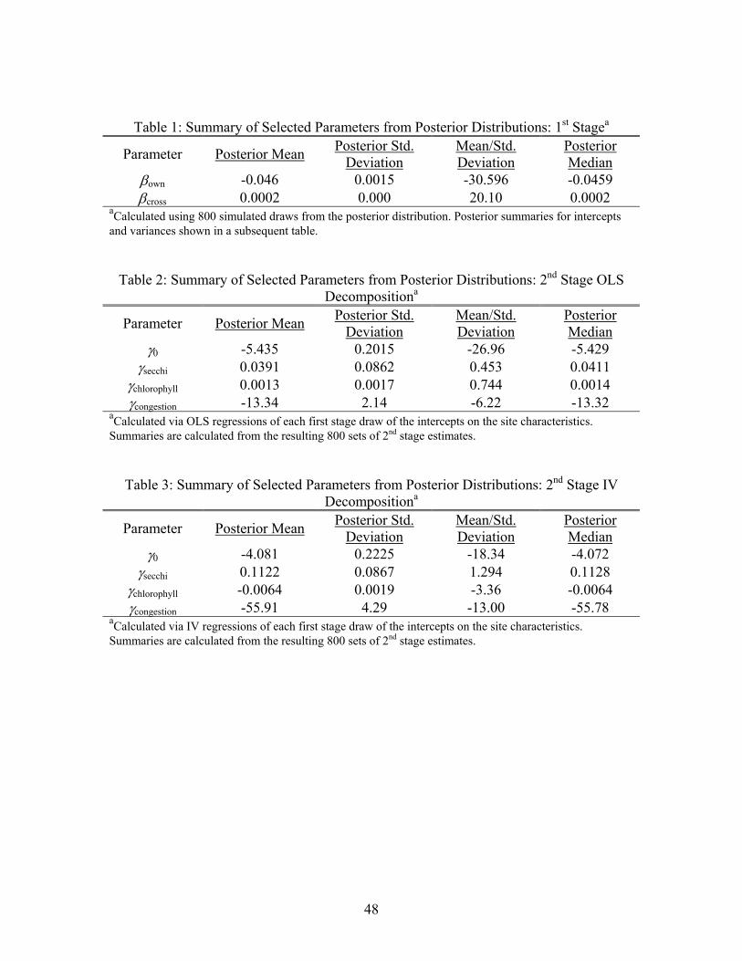
48

Table 1: Summary of Selected Parameters from Posterior Distributions: 1st Stagea

Parameter Posterior Mean Posterior Std. Deviation

Mean/Std. Deviation

Posterior Median

βown -0.046 0.0015 -30.596 -0.0459 βcross 0.0002 0.000 20.10 0.0002

aCalculated using 800 simulated draws from the posterior distribution. Posterior summaries for intercepts and variances shown in a subsequent table.

Table 2: Summary of Selected Parameters from Posterior Distributions: 2nd Stage OLS Decompositiona

Parameter Posterior Mean Posterior Std. Deviation

Mean/Std. Deviation

Posterior Median

γ0 -5.435 0.2015 -26.96 -5.429 γsecchi 0.0391 0.0862 0.453 0.0411

γchlorophyll 0.0013 0.0017 0.744 0.0014 γcongestion -13.34 2.14 -6.22 -13.32

aCalculated via OLS regressions of each first stage draw of the intercepts on the site characteristics. Summaries are calculated from the resulting 800 sets of 2nd stage estimates.

Table 3: Summary of Selected Parameters from Posterior Distributions: 2nd Stage IV Decompositiona

Parameter Posterior Mean Posterior Std. Deviation

Mean/Std. Deviation

Posterior Median

γ0 -4.081 0.2225 -18.34 -4.072 γsecchi 0.1122 0.0867 1.294 0.1128

γchlorophyll -0.0064 0.0019 -3.36 -0.0064 γcongestion -55.91 4.29 -13.00 -55.78

aCalculated via IV regressions of each first stage draw of the intercepts on the site characteristics. Summaries are calculated from the resulting 800 sets of 2nd stage estimates.

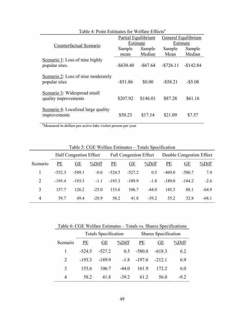
49

Table 4: Point Estimates for Welfare Effectsa

Partial Equilibrium Estimate

General Equilibrium Estimate Counterfactual Scenario Sample

mean Sample Median

Sample Mean

Sample Median

Scenario 1: Loss of nine highly popular sites.

-$630.40 -$67.64 -$726.11 -$142.84

Scenario 2: Loss of nine moderately popular sites

-$51.86 $0.00 -$58.21 -$5.08

Scenario 3: Widespread small quality improvements

$207.92 $146.01 $87.28 $61.16

Scenario 4: Localized large quality improvements

$50.23 $17.14 $21.09 $7.57

aMeasured in dollars per active lake visitor person per year

Table 5: CGE Welfare Estimates – Totals Specification Half Congestion Effect Full Congestion Effect Double Congestion Effect

Scenario PE GE %Diff PE GE %Diff PE GE %Diff

1 -552.3 -549.1 -0.6 -524.5 -527.2 0.5 -469.0 -506.7 7.4

2 -195.4 -193.3 -1.1 -193.3 -189.9 -1.8 -189.0 -184.2 -2.6

3 157.7 126.2 -25.0 153.6 106.7 -44.0 145.3 88.1 -64.9

4 59.7 49.4 -20.9 58.2 41.8 -39.2 55.2 32.8 -68.1

Table 6: CGE Welfare Estimates – Totals vs. Shares Specifications Totals Specification Shares Specification

Scenario PE GE %Diff PE GE %Diff

1 -524.5 -527.2 0.5 -580.0 -618.3 6.2

2 -193.3 -189.9 -1.8 -197.6 -212.1 6.9

3 153.6 106.7 -44.0 161.9 172.2 6.0

4 58.2 41.8 -39.2 61.2 56.0 -9.2

50

1 Recent notable exceptions are the equilibrium sorting models of [29], [30], and [5].

2 A similar approach was employed by Wang [34] and Pitt and Millimet [24].

3 In practice it is also necessary to check that the regimes implied by *tijz are in the feasible set

and, if not, adjust using the strategy discussed above. This emphasizes the point that using

predicted behavior to simulate new endogenous attribute outcomes also depends critically on the

ability to solve consumers’ outcomes accurately and quickly.

4 Appendix Figure B.1 provides histograms of the full marginal posterior distributions for the

price parameters in Table 1 and on the attributes for the specification in Table 3.

5 Appendix Table B.1 provides the posterior means and standard deviations for the sites-specific

intercepts and variance terms.

6 It is worth noting that, for this logic to be a complete description of the equilibrating process, it

must not be the case that this adjustment induces changes in the virtual prices at zero-visit sites.

If there were systematic changes in these prices across individuals in response to the policy, this

could complicate the equilibrium adjustment story described here.