Embed Size (px)
Citation preview
Non-perturbative solutions to
quasi-one-dimensional
strongly correlated systems
Submitted for the degree of Doctor of Philosophy
Sam T. Carr
St John’s College, University of Oxford
October, 2003

1
Don’t search for the answers, which could not be given to you now, because you
would not be able to live them. And the point is, to live everything. Live the ques-
tions now. Perhaps then, someday far in the future, you will gradually, without
even noticing it, live your way into the answer.
–Rilke
Abstract
In this thesis, we deal with quasi-one-dimensional field theories by which we mean strongly
anisotropic higher dimensional models. One way to solve such quasi-one-dimensional models
is to split them into a one-dimensional part and a weaker inter-chain perturbation on this.
The one-dimensional model can then be solved exactly by techniques such as bosonisation or
integrability, and the weak inter-chain part can be treatedperturbatively by using the Random
Phase Approximation (RPA), or beyond this. This allows us tocomment on concepts such
as dimensional crossover, and by treating the one-dimensional fluctuations exactly, we access
phases not accessible by conventional perturbation theory. In this thesis, we report results
for three such models: the first is a model of non-BCS superconductivity where a spin-gap
in the one dimensional chains leads to pairing, even for repulsive interactions. We look at
the interplay between a superconducting and a charge density wave ground state. The second
model is that of a Mott insulator, where we are specifically looking at the effects of a magnetic
field on the model. We look at the density of states as the angleof the magnetic field is varied.
The third system is the quantum Ising model, a generic model of two-state systems, where
we calculate the correlation functions in the ordered phase. All three models are motivated by
reference to real materials with a strong structural anisotropy.
Publications
1. S.T.Carr and A.M.Tsvelik : Superconductivity and charge density wave in a quasi-one-
dimensional spin gap system, Phys. Rev. B65, 195121 (2002) [1].
We consider a model of spin-gapped chains weakly coupled by Josephson and Coulomb
interactions. Combining such non-perturbative methods asbosonisation and Bethe ansatz
to treat the intra-chain interactions with the Random PhaseApproximation for the inter-
chain couplings and the first corrections to this, we investigate the phase diagram of
this model. The phase diagram shows both charge density waveordering and super-
conductivity. These phases are separated by a line of critical points which exhibits an
approximate an SU(2) symmetry. We consider the effects of a magnetic field on the
system. We apply the theory to the material Sr2Ca12Cu24O41 and suggest further exper-
iments.
2. S.T.Carr and A.M.Tsvelik : Spectrum and correlation functions of a quasi-one-dimensional
quantum Ising model, Phys. Rev. Lett. 90 177206 (2003) [2].
We consider a model of weakly coupled quantum Ising chains. We describe the phase
diagram of such a model and study the dynamical magnetic susceptibility by means
of Bethe ansatz and the Random Phase Approximation applied to the inter-chain ex-
change. We argue that some of the beautiful physics of the quantum Ising chain in a
magnetic field survives in the ordered state of the quasi-one-dimensional model and can
be observed experimentally by means of neutron scattering.
1

Acknowledgements
I would like to thank my friend and supervisor Alexei Tsvelikfor taking me as a student
and unveiling to me the world of physics through his eyes. Hisintuition in both physical
phenomena and mathematical problems as well as his interestin everything under the sun has
kept me constantly stimulated throughout my time working with him.
I would also like to thank Ralph Werner, Fabian Essler, MyronStrongin, Tim Kidd,
Florian Merz, Nic Shannon and Revaz Ramazashvili for many fruitful discussions as well as
all their friendship and support.
The department of theoretical physics, Oxford and department of condensed matter
physics, Brookhaven National Laboratory both offered me warm working environments, and
for financial support I have to thank both EPSRC and BNL.
Of course, one can’t live without friends; and to this end I thank all my friends for keep-
ing me sane during my time as a DPhil student, both in Oxford and New York. In particular
David, Laszlo, Zoe, Debbie, Darcy, Ken, Nora, Dan, Alex, Shela, Alison, David, Alison, Joe
and Christine.
In times of stress, I could always rely on Mozart to calm me down.
And finally, I have to thank my family: Nancy, Emily, Lemma, mummy and daddy for
continuous support and affection. Without you all I wouldn’t be here.
2
Contents
1 Introduction 5
2 Techniques in one dimension 8
2.1 Bosonisation . . . . . . . . . . . . . . . . . . . . . . . . . . . . . . . . . . 8
2.1.1 A heuristic view . . . . . . . . . . . . . . . . . . . . . . . . . . . . 8
2.1.2 The free boson and the free electron . . . . . . . . . . . . . . . .. . 10
2.1.3 Spin, interactions and the Luttinger model . . . . . . . . .. . . . . . 12
2.1.4 The sine-Gordon model and gap formation . . . . . . . . . . . .. . 16
2.2 Integrability . . . . . . . . . . . . . . . . . . . . . . . . . . . . . . . . . . .17
2.2.1 The S-matrix . . . . . . . . . . . . . . . . . . . . . . . . . . . . . . 18
2.2.2 Form-factors and correlation functions . . . . . . . . . . .. . . . . . 19
2.3 Conformal Field Theory . . . . . . . . . . . . . . . . . . . . . . . . . . . .21
2.4 From one dimension to quasi one dimension . . . . . . . . . . . . .. . . . . 23
3 Superconductors 24
3.1 Physical motivation . . . . . . . . . . . . . . . . . . . . . . . . . . . . . .. 24
3.2 The model . . . . . . . . . . . . . . . . . . . . . . . . . . . . . . . . . . . . 25
3.3 Low temperature phase diagram: Critical temperature and magnetic field effects 29
3.3.1 An Effective theory of the Critical Point . . . . . . . . . . .. . . . . 29
3.3.2 The Random Phase Approximation . . . . . . . . . . . . . . . . . . 30
3.3.3 Zero magnetic field; the critical temperature . . . . . . .. . . . . . . 33
3.3.4 Phase diagram in a magnetic field . . . . . . . . . . . . . . . . . . .35
3.4 Corrections to RPA . . . . . . . . . . . . . . . . . . . . . . . . . . . . . . . 37
3.5 Single Particle Spectral Function and other experimental signatures . . . . . . 39
3.5.1 Above the transition temperature . . . . . . . . . . . . . . . . .. . . 39
3.5.2 The ordered Phase . . . . . . . . . . . . . . . . . . . . . . . . . . . 41
3.6 A Word about Two Dimensions . . . . . . . . . . . . . . . . . . . . . . . . .43
3.7 Example experimental systems . . . . . . . . . . . . . . . . . . . . . .. . . 46
3.7.1 The telephone number compound . . . . . . . . . . . . . . . . . . . 46
3.7.2 β-Sodium Vanadate . . . . . . . . . . . . . . . . . . . . . . . . . . . 47
4 Mott Insulators 50
4.1 Physical Motivation . . . . . . . . . . . . . . . . . . . . . . . . . . . . . .. 50
3
CONTENTS 4
4.2 The Model and 1D Green’s Function . . . . . . . . . . . . . . . . . . . .. . 52
4.3 Inter-chain coupling and the magnetic field . . . . . . . . . . .. . . . . . . 54
4.3.1 RPA in the absence of a magnetic field . . . . . . . . . . . . . . . .. 54
4.3.2 Magnetic field parallel to chain direction . . . . . . . . . .. . . . . 55
4.3.3 Magnetic field perpendicular to chain direction . . . . .. . . . . . . 57
4.4 Density of states . . . . . . . . . . . . . . . . . . . . . . . . . . . . . . . . .57
4.5 Interpretation and Extensions to the model . . . . . . . . . . .. . . . . . . . 58
5 The quantum Ising model 64
5.1 The one dimensional quantum Ising model . . . . . . . . . . . . . .. . . . . 65
5.1.1 The model atT = 0 . . . . . . . . . . . . . . . . . . . . . . . . . . 65
5.1.2 The model at finite temperature - scaling behaviour . . .. . . . . . . 67
5.1.3 The critical model in a magnetic field . . . . . . . . . . . . . . .. . 68
5.2 The quasi-one-dimensional model . . . . . . . . . . . . . . . . . . .. . . . 69
5.2.1 The Phase Diagram . . . . . . . . . . . . . . . . . . . . . . . . . . . 70
5.2.2 Dispersion in the ordered phase . . . . . . . . . . . . . . . . . . .. 71
5.3 Application toα’ Sodium Vanadate . . . . . . . . . . . . . . . . . . . . . . 74
5.4 Link to the 3D Ising Model . . . . . . . . . . . . . . . . . . . . . . . . . . .76
6 Final remarks 77
Chapter 1
Introduction
“Begin at the beginning,” the King said gravely, ”and go on till you come to the
end: then stop”.
–Lewis Carroll
The topic of strong correlations in condensed matter physics is a fascinating story of
mystery and surprise.
To understand strong correlations we must first understand weakly correlated systems,
for example Fermi liquid theory [3, 4]. The easiest thing to do as a first approximation in
an interacting field theory is to simply ignore the interactions. It turns out in many models
of condensed matter physics, this rather drastic looking step is not such a bad thing to do.
The effect of ’weak’ interactions is merely to renormalize the excitations (quasi-particles) of
the non-interacting system. Basically, this means that youmap your model of interacting
electrons onto a model of free electron like particles, where properties such as mass are a
parameter different from the bare (free) electron mass. Because nothing unusual happens,
one can calculate these effective parameters from the original theory as a perturbation series;
where including more terms gives a more accurate result.
A strongly-correlated system is a system where we can not do this; the interactions
change the nature of the ground-state and/or the quantum numbers of the excitation spectrum.
It is not possible to obtain the characteristics of the system perturbatively by smoothly switch-
ing on the interaction from the free model.
We must then say what it means to ’solve’ such a model. This requires in a certain region
of parameter space mapping the model onto a weakly-interacting systems, where you can then
read off the ground state and excitation spectra and quantumnumbers. The residual interac-
tions can be treated perturbatively and do not give any qualitative change to the results. We
must stress that in most cases this can only be done in certainlocalised regions of parameter
space. Elsewhere, the spectrum may be (and usually is) completely different.
There are two ways of solving physical problems in condensedmatter: a ’top-down’ and
a ’bottom-up’ approach. In the ’bottom-up’ approach, one writes down some exact Hamilto-
nian for the system and then tries to approximately solve it using powerful computation tech-
niques. This is in some sense the most fundamental approach.You start with no assumptions
5
CHAPTER 1. INTRODUCTION 6
about your system and you see what you can find out. This can be very satisfying when it gives
correct answers for questions such as the band-gap in semiconductors. However, it will often
offer very little physical insight into the system. For this, the top-down approach is preferred.
You start by looking at your system and making some guess as towhat the important physical
features of it are. You then construct some simplified Hamiltonian retaining these features
which you then hope to be able to solve analytically.
In this thesis, the feature that we concentrate on is a strongstructural anisotropy of
hopping or interactions meaning that the system is effectively one-dimensional. Our model
Hamiltonian is therefore going to be one-dimensional.
There are many interesting features of one dimensional models. Firstly, interaction ef-
fects are usually much stronger. This can be understood verynaively by simple phase space
arguments: two particles in two or more dimensions have to betravelling at a specific angle
to ’collide’ with each other. In one dimension, merely having different velocities is sufficient
to ensure eventual meeting. Secondly, there are a wealth of techniques available to come up
with exact solutions of one-dimensional models, so we can accurately say what our model
Hamiltonian predicts about the system in question, and thensay any discrepancies are due to
our model being over-simplified rather than an incorrect or incomplete solution to the model.
Of course, a true one-dimensional model is almost always over-simplified when trying to
describe a three dimensional solid. Most importantly, three dimensional crystals show phase
transitions, whereas one dimensional ones do not. So for many purposes we need to extend
our exactly solvable one-dimensional models to have some weak inter-chain coupling before
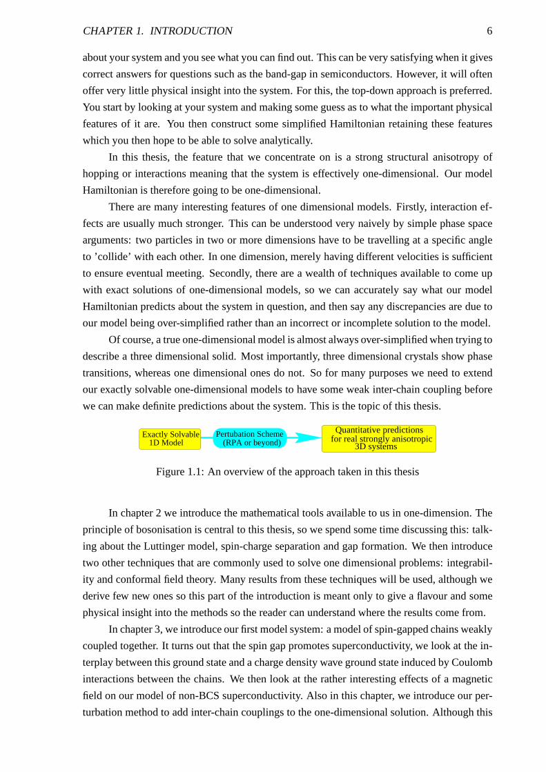
we can make definite predictions about the system. This is thetopic of this thesis.
Quantitative predictionsfor real strongly anisotropic
3D systemsExactly Solvable
1D ModelPertubation Scheme
(RPA or beyond)
Figure 1.1: An overview of the approach taken in this thesis
In chapter 2 we introduce the mathematical tools available to us in one-dimension. The
principle of bosonisation is central to this thesis, so we spend some time discussing this: talk-
ing about the Luttinger model, spin-charge separation and gap formation. We then introduce
two other techniques that are commonly used to solve one dimensional problems: integrabil-
ity and conformal field theory. Many results from these techniques will be used, although we
derive few new ones so this part of the introduction is meant only to give a flavour and some
physical insight into the methods so the reader can understand where the results come from.
In chapter 3, we introduce our first model system: a model of spin-gapped chains weakly
coupled together. It turns out that the spin gap promotes superconductivity, we look at the in-
terplay between this ground state and a charge density wave ground state induced by Coulomb
interactions between the chains. We then look at the rather interesting effects of a magnetic
field on our model of non-BCS superconductivity. Also in thischapter, we introduce our per-
turbation method to add inter-chain couplings to the one-dimensional solution. Although this
CHAPTER 1. INTRODUCTION 7
is a perturbation theory, it is not in interaction strength as the one dimensional interactions are
treated exactly. In this sense, the method is rather confusingly known as a non-perturbative
solution. This allows us to see possibilities not accessible by conventional perturbation the-
ory, and allows us to comment on phenomena such as non-Fermi-liquids and dimensional
crossover.
Chapter 4 then goes on to look at a complimentary model, wherethe one-dimensional
chains have a charge-gap rather than a spin-gap, i.e. the chains are Mott Insulators (meaning
that the insulating behaviour comes from the electron-electron interactions rather than band
structure). It turns out that adding an inter-chain hoppingterm to this system can drive it to a
rather unusual metallic state. The central question in thischapter is what happens to this state
in a magnetic field, a question very pertinent to recent experimental results.
Finally, in chapter 5, we look at a quasi-one-dimensional spin-chain model. A large
number of interesting results are known about the quantum Ising model in one-dimension, our
question here is how robust are some of these results againstinter-chain interactions. When
we form an ordered phase, it is necessarily three-dimensional, but in this chapter we show that
for certain regions of parameter space this ordered phase will show a lot of one dimensional
properties, a signature that should be visible in experimental results.
In each chapter, we try to motivate and support the model withreference to real materials
to which the model could be at least partially applied. It wasthe original aim of this work
to then fully apply our solutions to these materials to attempt to come up with quantitative
predictions about the materials. Unfortunately, the complexity of the materials we talk about
in this thesis means that such detailed calculations are outside the scope of this work. However,
we believe that a solution of the underlying models is a good starting point for any attempt to
accurately describe these materials.
Chapter 2
Techniques in one dimension
As far as the laws of mathematics refer to reality, they are not certain, and as far
as they are certain, they do not refer to reality.–A. Einstein
One dimensional models are the perfect place to explore the effects of strong correla-
tions. Not only are the effects of correlations the strongest, there also exists a wealth of math-
ematical techniques which facilitate the study of such systems. The three main techniques are
as follows:
1. Bosonisation, which comes about from the low energy excitations in a 1D Fermi liquid
being limited to the vicinity of the two Fermi points,
2. Exact solutions of integrable models which have the property that the scattering matrix
factorises due to strong kinematic constraints in one dimension, and
3. Conformal Field Theory (CFT), which comes from special properties of the conformal
group in 1+1D and is useful for critical phenomena.
The first of these points is central to most of the thesis, so wespend some time discussing it.
Many results from integrability and CFT will be used although we derive no new ones so we
simply give a brief overview of what each of these techniquesinvolves.
2.1 Bosonisation
For one-dimensional field theories of interacting electrons, bosonisation is usually the starting
point. We begin by giving some physical intuition why this isa good idea in one dimension,
then go on to derive the mathematical relations between an interacting Fermi system and a
Bosonic model. This also serves to introduce the notation used throughout much of this thesis.
2.1.1 A heuristic view
In a one dimensional system, the Fermi surface is simply two points. A low energy excitation
above the ground state involves taking an electron near one of these points, and exciting it
8
CHAPTER 2. TECHNIQUES IN ONE DIMENSION 9
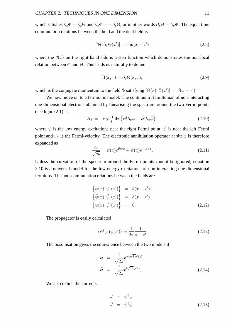
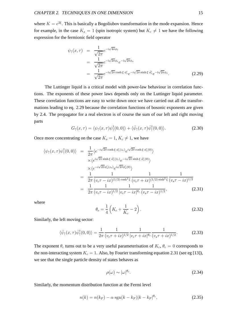
π0 k
k
F
εF
–kF
ε(k)
k
E
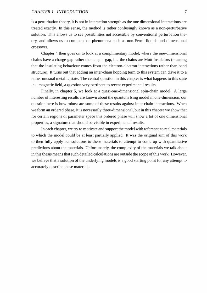
Figure 2.1: Particle/hole excitations in a 1D electron system. Because the Fermi surfaceis simply two points, the low energy low-momentum excitation spectrum collapses onto anarrow line. The width is related to the curvature of the spectrum at the Fermi-points, sobecomes zero if one linearises the spectrum - see the text. After [5].
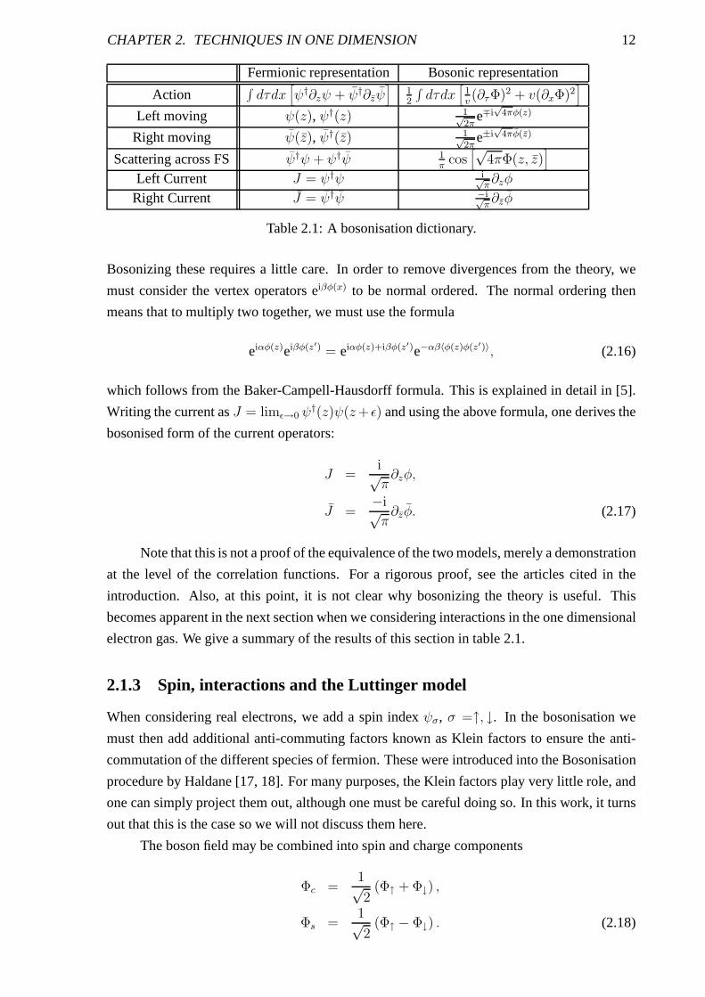
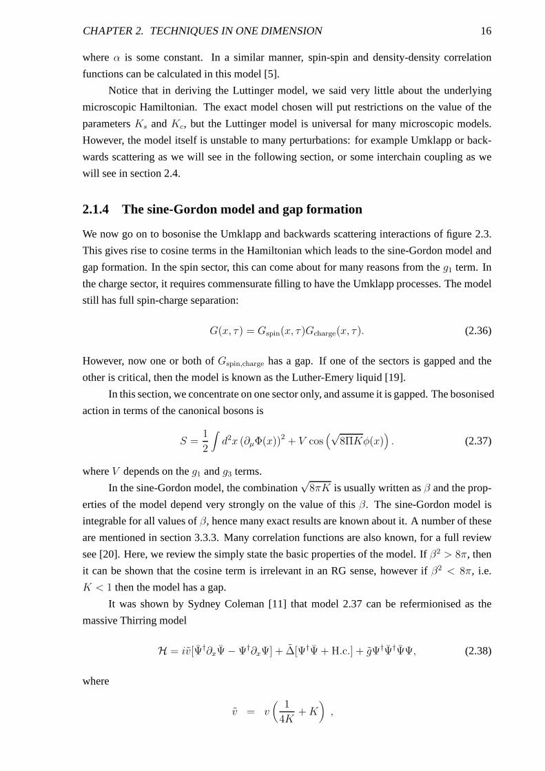
k
Ek
k
kx
ky
kF
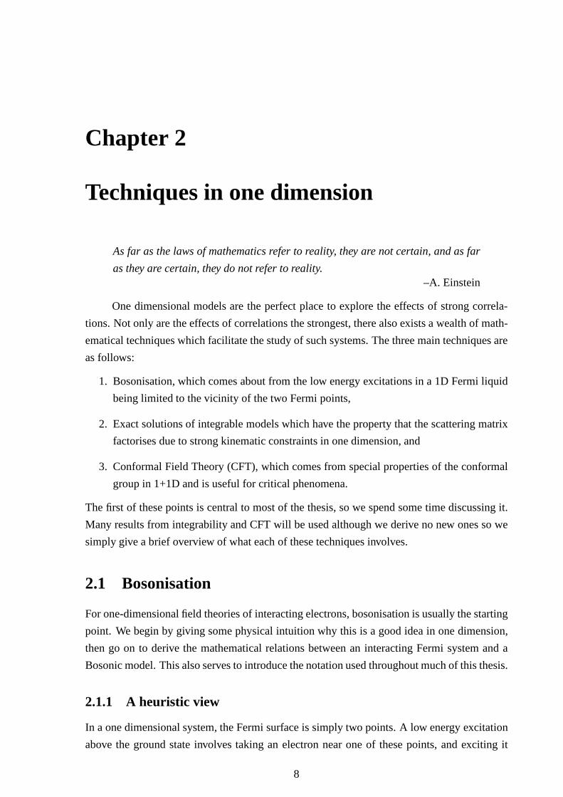
Figure 2.2: Particle-hole excitations in a 2D electron system. k is the momentum in somedirection, the full spectrum would be found by rotating the graph about it’s origin into thepage. Because of the choice of angle for the excitations, there is a continuum of low-energyparticle hole excitations, meaning that the particle and hole must be considered as independentexcitations. After [5].
to a vacant spot just outside the Fermi surface, leaving a hole. The momentum transfer is
q = ke − kh and the energy isǫq = Ee − Eh. As shown in figure 2.1, the low energy
excitations are then a coherent state of the electron and thehole, and so the excitation can be
considered a single bosonic state. In two or three dimensions, there will be a range ofǫq to
go with any one momentum transfer (figure 2.2), so one must still consider the excitations as
independent particles and holes.
The power of bosonisation is that upon adding certain electron-electron (e-e) interactions
it turns out that the bosons are robust (naively because the interactions affect the particles and
holes in similar ways). Although it is then difficult to say how the excitations are made out of
the original electrons, we find they are renormalised bosonsrather than renormalised fermions
as in Fermi-liquid theory. This is the essence of bosonisation, it is all made rather more
concrete in the next section.
As a historical aside, it was realised by Bloch as early as 1934 that hole-electron pairs
are bosonic in nature, but it was Tomonaga in 1950 [6] who firstshowed that these were
elementary excitations in one dimension. Luttinger then proposed a one-dimensional model
[7] which was solved by a method similar to today’s bosonisation procedure by Mattis and
Leib [8]. The first modern field-theoretic approach to bosonisation was given by Heidenreich
et. al. [9] and gave the solution to the model proposed by Luther and Peschel [10]. Around
the same time, the same ideas were being developed starting from the equivalence between
the sine-Gordon and massive Thirring models [11, 12]. Thereare a number of good reviews
CHAPTER 2. TECHNIQUES IN ONE DIMENSION 10
of the bosonisation procedure, for example Tsvelik, Nersesyan and Gogolin [13] or Emery
[14]. Another good and very complete review is von Delft and Schoeller [15], but the one we
follow closest is Senechal [5] who uses the field theory formulation. In this section, we do
not attempt to give a proof of the procedure, but merely give the basics with as much physical
motivation as possible.
2.1.2 The free boson and the free electron
To show the equivalence between an electronic model and a bosonic model, we first consider
the relevant properties of the bosonic Gaussian model defined by the action
S =1
2
∫
dτdx[
1
v(∂τΦ)2 + v(∂xΦ)2
]
, (2.1)
whereτ is Matsubara time,v is a velocity andΦ is a scaler bosonic field. AtT = 0, it is
relatively simple to show (see eg [16]) that the single particle Green’s function is
G(z, z) = 〈Φ(z, z)Φ(0, 0)〉 =1
4πln
(
R2
zz + a20
)
, (2.2)
wherez = x + iτ , R is the system size anda0 is the lattice spacing which are introduced to
regularise the system. Now, defining the correlation functions of bosonic exponents:
F (1, 2, . . . , N) = 〈eiβ1Φ(ξ1) . . .eiβNΦ(ξN )〉, (2.3)
we find that (see [13] for details)
F (1, 2, . . . , N) =∏
i>j
(
zij zija2
0
)βiβj/4π (R
a0
)−(∑
iβi)
2/4π
. (2.4)
For an infinite system,R → ∞ and we get the neutrality condition that the correlation function
of exponents is only non-zero if∑
i
βi = 0. (2.5)
We see that the propagator factorises into independent leftand right moving parts, which are
functions ofz andz only respectively. Hence we can define the chiral componentsof the field
Φ(z, z) = φ(z) + φ(z), (2.6)
and consider correlation functions of eiβφ and eiβφ separately. We must understand however,
that this factorisation is a property of the correlation functions only and not a restriction onΦ
in a path integral. We also define the dual field
Θ(z, z) = φ(z) − φ(z), (2.7)
CHAPTER 2. TECHNIQUES IN ONE DIMENSION 11
which satisfies∂zΦ = ∂zΘ and∂zΦ = −∂zΘ, or in other words∂xΘ = ∂τΦ. The equal time
commutation relations between the field and the dual field is
[Φ(x),Θ(x′)] = −iθ(x − x′) (2.8)
where theθ(x) on the right hand side is a step function which demonstrates the non-local
relation betweenΦ andΘ. This leads us naturally to define
Π(x, τ) = ∂xΘ(x, τ), (2.9)
which is the conjugate momentum to the fieldΦ satisfying[Θ(x),Φ(x′)] = iδ(x− x′).
We now move on to a fermionic model. The continuum Hamiltonian of non-interacting
one-dimensional electrons obtained by linearising the spectrum around the two Fermi points
(see figure 2.1) is
HF = −ivF
∫
dx(
ψ†∂xψ − ψ†∂xψ)
, (2.10)
whereψ is the low energy excitations near the right Fermi point,ψ is near the left Fermi
point andvF is the Fermi-velocity. The electronic annihilation operator at sitex is therefore
expanded ascx√a0
= ψ(x)eikFx + ψ(x)e−ikF x. (2.11)
Unless the curvature of the spectrum around the Fermi pointscannot be ignored, equation
2.10 is a universal model for the low-energy excitations of non-interacting one dimensional
fermions. The anti-commutation relations between the fields are
{
ψ(x), ψ†(x′)}
= δ(x− x′),{
ψ(x), ψ†(x′)}
= δ(x− x′),{
ψ(x), ψ†(x′)}
= 0. (2.12)
The propagator is easily calculated
〈ψ†(z)ψ(z′)〉 =1
2π
1
z − z′(2.13)
The bosonisation gives the equivalence between the two models if
ψ =1√2π
e−i√
4πφ(z),
ψ =1√2π
ei√
4πφ(z), (2.14)
We also define the currents
J = ψ†ψ,
J = ψ†ψ. (2.15)
CHAPTER 2. TECHNIQUES IN ONE DIMENSION 12
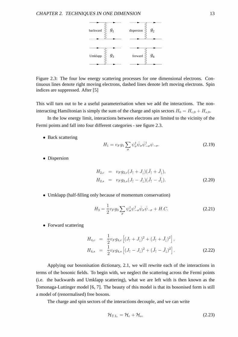
Fermionic representation Bosonic representation
Action∫
dτdx[
ψ†∂zψ + ψ†∂zψ]
12
∫
dτdx[
1v(∂τΦ)2 + v(∂xΦ)2
]
Left moving ψ(z), ψ†(z) 1√2π
e∓i√
4πφ(z)
Right moving ψ(z), ψ†(z) 1√2π
e±i√
4πφ(z)
Scattering across FS ψ†ψ + ψ†ψ 1π
cos[√
4πΦ(z, z)]
Left Current J = ψ†ψ i√π∂zφ
Right Current J = ψ†ψ −i√π∂zφ
Table 2.1: A bosonisation dictionary.
Bosonizing these requires a little care. In order to remove divergences from the theory, we
must consider the vertex operators eiβφ(x) to be normal ordered. The normal ordering then
means that to multiply two together, we must use the formula
eiαφ(z)eiβφ(z′) = eiαφ(z)+iβφ(z′)e−αβ〈φ(z)φ(z′)〉, (2.16)
which follows from the Baker-Campell-Hausdorff formula. This is explained in detail in [5].
Writing the current asJ = limǫ→0 ψ†(z)ψ(z+ ǫ) and using the above formula, one derives the
bosonised form of the current operators:
J =i√π∂zφ,
J =−i√π∂zφ. (2.17)
Note that this is not a proof of the equivalence of the two models, merely a demonstration
at the level of the correlation functions. For a rigorous proof, see the articles cited in the
introduction. Also, at this point, it is not clear why bosonizing the theory is useful. This
becomes apparent in the next section when we considering interactions in the one dimensional
electron gas. We give a summary of the results of this sectionin table 2.1.
2.1.3 Spin, interactions and the Luttinger model
When considering real electrons, we add a spin indexψσ, σ =↑, ↓. In the bosonisation we
must then add additional anti-commuting factors known as Klein factors to ensure the anti-
commutation of the different species of fermion. These wereintroduced into the Bosonisation
procedure by Haldane [17, 18]. For many purposes, the Klein factors play very little role, and
one can simply project them out, although one must be carefuldoing so. In this work, it turns
out that this is the case so we will not discuss them here.
The boson field may be combined into spin and charge components
Φc =1√2
(Φ↑ + Φ↓) ,
Φs =1√2
(Φ↑ − Φ↓) . (2.18)
CHAPTER 2. TECHNIQUES IN ONE DIMENSION 13
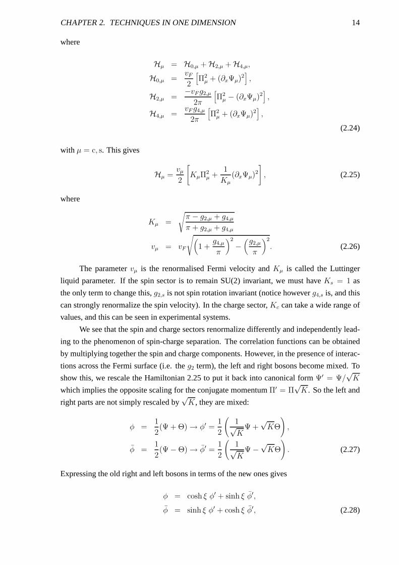
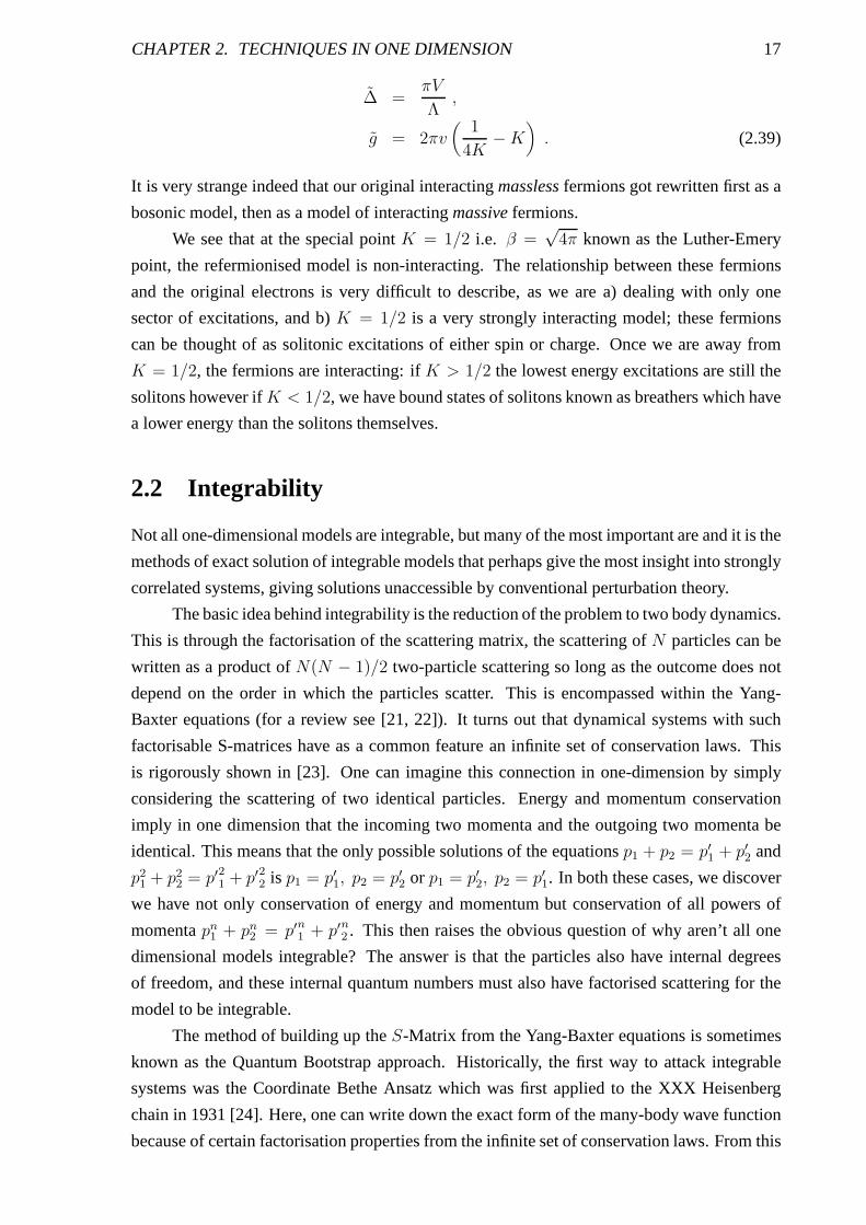
g1 g2
g3 g4
backward dispersion
forwardUmklapp
Figure 2.3: The four low energy scattering processes for onedimensional electrons. Con-tinuous lines denote right moving electrons, dashed lines denote left moving electrons. Spinindices are suppressed. After [5]
This will turn out to be a useful parameterisation when we addthe interactions. The non-
interacting Hamiltonian is simply the sum of the charge and spin sectorsH0 = Hc,0 +Hs,0.
In the low energy limit, interactions between electrons arelimited to the vicinity of the
Fermi points and fall into four different categories - see figure 2.3.
• Back scattering
H1 = vF g1
∑
σ
ψ†σψσψ
†−σψ−σ. (2.19)
• Dispersion
H2,c = vFg2,c(J↑ + J↓)(J↑ + J↓),
H2,s = vFg2,s(J↑ − J↓)(J↑ − J↓). (2.20)
• Umklapp (half-filling only because of momentum conservation)
H3 =1
2vFg3
∑
σ
ψ†σψ
†−σψσψ−σ +H.C. (2.21)
• Forward scattering
H4,c =1
2vFg4,c
[
(J↑ + J↓)2 + (J↑ + J↓)
2]
,
H4,s =1
2vFg4,s
[
(J↑ − J↓)2 + (J↑ − J↓)
2]
. (2.22)
Applying our bosonisation dictionary, 2.1, we will rewriteeach of the interactions in
terms of the bosonic fields. To begin with, we neglect the scattering across the Fermi points
(i.e. the backwards and Umklapp scattering), what we are left with is then known as the
Tomonaga-Luttinger model [6, 7]. The beauty of this model isthat its bosonised form is still
a model of (renormalised) free bosons.
The charge and spin sectors of the interactions decouple, and we can write
HT.L. = Hc + Hs, (2.23)
CHAPTER 2. TECHNIQUES IN ONE DIMENSION 14
where
Hµ = H0,µ + H2,µ + H4,µ,
H0,µ =vF2
[
Π2µ + (∂xΨµ)
2]
,
H2,µ =−vF g2,µ
2π
[
Π2µ − (∂xΨµ)
2]
,
H4,µ =vF g4,µ
2π
[
Π2µ + (∂xΨµ)
2]
,
(2.24)
with µ = c, s. This gives
Hµ =vµ2
[
KµΠ2µ +
1
Kµ
(∂xΨµ)2
]
, (2.25)
where
Kµ =
√
π − g2,µ + g4,µ
π + g2,µ + g4,µ
vµ = vF
√
(
1 +g4,µ
π
)2
−(
g2,µ
π
)2
. (2.26)
The parametervµ is the renormalised Fermi velocity andKµ is called the Luttinger
liquid parameter. If the spin sector is to remain SU(2) invariant, we must haveKs = 1 as
the only term to change this,g2,s is not spin rotation invariant (notice howeverg4,s is, and this
can strongly renormalize the spin velocity). In the charge sector,Kc can take a wide range of
values, and this can be seen in experimental systems.
We see that the spin and charge sectors renormalize differently and independently lead-
ing to the phenomenon of spin-charge separation. The correlation functions can be obtained
by multiplying together the spin and charge components. However, in the presence of interac-
tions across the Fermi surface (i.e. theg2 term), the left and right bosons become mixed. To
show this, we rescale the Hamiltonian 2.25 to put it back intocanonical formΨ′ = Ψ/√K
which implies the opposite scaling for the conjugate momentumΠ′ = Π√K. So the left and
right parts are not simply rescaled by√K, they are mixed:
φ =1
2(Ψ + Θ) → φ′ =
1
2
(
1√K
Ψ +√KΘ
)
,
φ =1
2(Ψ − Θ) → φ′ =
1
2
(
1√K
Ψ −√KΘ
)
. (2.27)
Expressing the old right and left bosons in terms of the new ones gives
φ = cosh ξ φ′ + sinh ξ φ′,
φ = sinh ξ φ′ + cosh ξ φ′, (2.28)
CHAPTER 2. TECHNIQUES IN ONE DIMENSION 15
whereK = e2ξ. This is basically a Bogoliubov transformation in the mode expansion. Hence
for example, in the caseKs = 1 (spin isotropic system) butKc 6= 1 we have the following
expression for the fermionic field operator
ψ↑(x, τ) =1√2πe−i
√4πφ↑
=1√2πe−i
√2πφce−i
√2πφs
=1√2πe−i
√2π cosh ξ φ′ce−i
√2π sinh ξ φ′ce−i
√2πφs. (2.29)
The Luttinger liquid is a critical model with power-law behaviour in correlation func-
tions. The exponents of these power laws depends only on the Luttinger liquid parameter.
These correlation functions are easy to write down once we have carried out all the transfor-
mations leading to eq. 2.29 because the correlation functions of bosonic exponents are given
by 2.4. The propagator for a real electron is of course the sumof our left and right moving
parts
G↑(x, τ) = 〈ψ↑(x, τ)ψ†↑(0, 0)〉 + 〈ψ↑(x, τ)ψ
†↑(0, 0)〉. (2.30)
Once more concentrating on the caseKs = 1,Kc 6= 1, we have
〈ψ↑(x, τ)ψ†↑(0, 0)〉 =
1
2π〈e−i
√2π cosh ξ φ′c(zc)ei
√2π cosh ξ φ′c(0)〉
×〈ei√
2π sinh ξ φ′c(zc)e−i√
2π sinh ξ φ′c(0)〉×〈e−i
√2πφ′s(zs)ei
√2πφ′s(0)〉
=1
2π
1
(vcτ − ix)(1/2) cosh2 ξ
1
(vcτ + ix)(1/2) sinh2 ξ
1
(vsτ − ix)1/2
=1
2π
1
(vcτ − ix)1/2
1
|vcτ − ix|θc
1
(vsτ − ix)1/2, (2.31)
where
θc =1
4
(
Kc +1
Kc− 2
)
. (2.32)
Similarly, the left moving sector:
〈ψ↑(x, τ)ψ†↑(0, 0)〉 =
1
2π
1
(vcτ + ix)1/2
1
|vcτ + ix|θc
1
(vsτ + ix)1/2. (2.33)
The exponentθc turns out to be a very useful parameterisation ofKc, θc = 0 corresponds to
the non-interacting systemKc = 1. Also, by Fourier transforming equation 2.31 (see eg [13]),
we see that the single particle density of states behaves as
ρ(ω) ∼ |ω|θc. (2.34)
Similarly, the momentum distribution function at the Fermilevel
n(k) = n(kF ) − α sgn(k − kF )|k − kF |θc , (2.35)
CHAPTER 2. TECHNIQUES IN ONE DIMENSION 16
whereα is some constant. In a similar manner, spin-spin and density-density correlation
functions can be calculated in this model [5].
Notice that in deriving the Luttinger model, we said very little about the underlying
microscopic Hamiltonian. The exact model chosen will put restrictions on the value of the
parametersKs andKc, but the Luttinger model is universal for many microscopic models.
However, the model itself is unstable to many perturbations: for example Umklapp or back-
wards scattering as we will see in the following section, or some interchain coupling as we
will see in section 2.4.
2.1.4 The sine-Gordon model and gap formation
We now go on to bosonise the Umklapp and backwards scatteringinteractions of figure 2.3.
This gives rise to cosine terms in the Hamiltonian which leads to the sine-Gordon model and
gap formation. In the spin sector, this can come about for many reasons from theg1 term. In
the charge sector, it requires commensurate filling to have the Umklapp processes. The model
still has full spin-charge separation:
G(x, τ) = Gspin(x, τ)Gcharge(x, τ). (2.36)
However, now one or both ofGspin,charge has a gap. If one of the sectors is gapped and the
other is critical, then the model is known as the Luther-Emery liquid [19].
In this section, we concentrate on one sector only, and assume it is gapped. The bosonised
action in terms of the canonical bosons is
S =1
2
∫
d2x (∂µΦ(x))2 + V cos(√
8ΠKφ(x))
. (2.37)
whereV depends on theg1 andg3 terms.
In the sine-Gordon model, the combination√
8πK is usually written asβ and the prop-
erties of the model depend very strongly on the value of thisβ. The sine-Gordon model is
integrable for all values ofβ, hence many exact results are known about it. A number of these
are mentioned in section 3.3.3. Many correlation functionsare also known, for a full review
see [20]. Here, we review the simply state the basic properties of the model. Ifβ2 > 8π, then
it can be shown that the cosine term is irrelevant in an RG sense, however ifβ2 < 8π, i.e.
K < 1 then the model has a gap.
It was shown by Sydney Coleman [11] that model 2.37 can be refermionised as the
massive Thirring model
H = iv[Ψ†∂xΨ − Ψ†∂xΨ] + ∆[Ψ†Ψ + H.c.] + gΨ†Ψ†ΨΨ, (2.38)
where
v = v(
1
4K+K
)
,
CHAPTER 2. TECHNIQUES IN ONE DIMENSION 17
∆ =πV
Λ,
g = 2πv(
1
4K−K
)
. (2.39)
It is very strange indeed that our original interactingmasslessfermions got rewritten first as a
bosonic model, then as a model of interactingmassivefermions.
We see that at the special pointK = 1/2 i.e. β =√
4π known as the Luther-Emery
point, the refermionised model is non-interacting. The relationship between these fermions
and the original electrons is very difficult to describe, as we are a) dealing with only one
sector of excitations, and b)K = 1/2 is a very strongly interacting model; these fermions
can be thought of as solitonic excitations of either spin or charge. Once we are away from
K = 1/2, the fermions are interacting: ifK > 1/2 the lowest energy excitations are still the
solitons however ifK < 1/2, we have bound states of solitons known as breathers which have
a lower energy than the solitons themselves.
2.2 Integrability
Not all one-dimensional models are integrable, but many of the most important are and it is the
methods of exact solution of integrable models that perhapsgive the most insight into strongly
correlated systems, giving solutions unaccessible by conventional perturbation theory.
The basic idea behind integrability is the reduction of the problem to two body dynamics.
This is through the factorisation of the scattering matrix,the scattering ofN particles can be
written as a product ofN(N − 1)/2 two-particle scattering so long as the outcome does not
depend on the order in which the particles scatter. This is encompassed within the Yang-
Baxter equations (for a review see [21, 22]). It turns out that dynamical systems with such
factorisable S-matrices have as a common feature an infiniteset of conservation laws. This
is rigorously shown in [23]. One can imagine this connectionin one-dimension by simply
considering the scattering of two identical particles. Energy and momentum conservation
imply in one dimension that the incoming two momenta and the outgoing two momenta be
identical. This means that the only possible solutions of the equationsp1 + p2 = p′1 + p′2 and
p21 + p2
2 = p′21 + p′22 is p1 = p′1, p2 = p′2 or p1 = p′2, p2 = p′1. In both these cases, we discover
we have not only conservation of energy and momentum but conservation of all powers of
momentapn1 + pn2 = p′n1 + p′n2 . This then raises the obvious question of why aren’t all one
dimensional models integrable? The answer is that the particles also have internal degrees
of freedom, and these internal quantum numbers must also have factorised scattering for the
model to be integrable.
The method of building up theS-Matrix from the Yang-Baxter equations is sometimes
known as the Quantum Bootstrap approach. Historically, thefirst way to attack integrable
systems was the Coordinate Bethe Ansatz which was first applied to the XXX Heisenberg
chain in 1931 [24]. Here, one can write down the exact form of the many-body wave function
because of certain factorisation properties from the infinite set of conservation laws. From this
CHAPTER 2. TECHNIQUES IN ONE DIMENSION 18
wave-function, one can calculate physical properties of the system. A third method is based
on the algebraic structure of the factorisation equations and is known as the Algebraic Bethe
Ansatz, or the Quantum Inverse Scattering Method. This is fully reviewed in [25]. All of
these methods are equivalent, although each have their advantages and disadvantages in terms
of calculation techniques.
2.2.1 The S-matrix
The S-matrix is the heart of an integrable model. It is represented pictorially as
S12 = 1 2
time
We will mostly be dealing with theories with Lorentz invariance, so we parameterise the
energy and momentum by the rapidityθ:
E = m cosh θ,
p = m sinh θ, (2.40)
so scattering between two particles is simply a function ofθ12 = θ1 − θ2. We also note here
thatθ → θ + iπ changesE → −E, p → p so this can be considered as changing a particle
into its antiparticle.
The Yang-Baxter factorisation equations are the most important property of the inte-
grable model. They can be represented pictorially as
1 2 3 1 2 3
=
S12(θ12)S13(θ13)S23(θ23) = S23(θ23)S13(θ13)S12(θ12). (2.41)
Basically what this is saying is that if three particles scatter off each other, it doesn’t matter
which order they do so in.
For a well defined theory, theS-matrix must be unitary:
=
1 2 1 2
1 = S12(θ12)S21(θ21). (2.42)
These conditions are also true for non-relativistic theories if we parameterise the scatter-
ing by the momentum transfer rather than the rapidity. The final condition, crossing-symmetry
is a purely relativistic effect, which is represented as
CHAPTER 2. TECHNIQUES IN ONE DIMENSION 19
= =
S12(θ12) = S21(θ21 + iπ) = S21(θ21 − iπ). (2.43)
There are also a number of properties relating to the formation of bound states. A bound
state shows up as a pole in the S-matrix, which means that if there are no bound states, then the
S-matrix must have no poles in the physical sheet (i.e.0 < Imθ < π. For more information
on the bound states, see for example [26].
These properties are enough to exactly determine theS-matrix, which can then be used
to determine many observable properties of the system. We give only one extremely simple
example which will be used later in this thesis, for the one dimensional Quantum Ising Model
(section 5.1).
H = −J∑
n
{
σznσzn+1 + (1 + g)σxn
}
. (2.44)
In this case, the Jordan-Wigner transformation reduces themodel to free fermions. Hence the
asymptotic states are free fermions so the scattering matrix is trivial:
S = −1. (2.45)
2.2.2 Form-factors and correlation functions
Form factors are off-shell scattering amplitudes
FOǫ1...ǫn(θ1, . . . , θn) = 〈0|O|θ1, . . . θn〉ǫ1...ǫn, (2.46)
whereθn are the rapidities of some excitations in the system andǫn denotes other internal
quantum numbers. These are simply matrix elements of the operatorO with various excited
states, however the expression 2.46 is limited to integrable models for the following reason.
If one doesn’t have factorised scattering, then multi-particle excitations can not be simply
written in terms of the rapidities of each excitations, thisis an incomplete parameterisation of
the state.
The form factors can be calculated in a bootstrap approach similar to theS-matrix [20,
27, 28, 26]. Again the equations come about as consequences of the factorisation of the
S-matrix. Firstly, the end result of annihilating the excitations by the operatorO must be
the same as if two of them scatter first. This is known as Watson’s equation, and can be
represented pictorially as:
�� � O. . . . . . =
�� � O
��A
A. . . . . . (2.47)
FO...ij...(. . . , θi, θj , . . .) = FO
...ji...(. . . , θj , θi, . . .)Sij(θi − θj). (2.48)
CHAPTER 2. TECHNIQUES IN ONE DIMENSION 20
Changing particles to anti-particles, we get conditions known as crossing relations which
can be represented:
�� � Oconn.. . .
= � �� � O
. . .= � �� � O. . .
(2.49)
ǫ1〈 θ1 | O(0) | p2, . . . , pn 〉in,conn.ǫ2...ǫn= FO
ǫ1ǫ2...ǫn(θ1 + iπ, θ2, . . . , θn) (2.50)
= FOǫ2...ǫnǫ1
(θ2, . . . , θn, θ1 − iπ). (2.51)
Finally, we can relate form-factors with different numbersof excitations by a recursion
relation:
1
2iResθ12=iπ
�� � O. . .
= ���� � O. . .
−
# !�
�� � O. . . (2.52)
Resθ12=iπFO1...n(θ1, . . .) = 2iC12 F
O3...n(θ3, . . .) (1 − S2n . . . S23) , (2.53)
whereC12 is the charge conjugation matrix with elementsCαα′ = δαα′ which basically ensures
charge conservation in the above expression. In words, whatthis expression is saying is that
the particles all being annihilated by the operatorO is equivalent to two of them annihilating
each other and the rest being annihilated byO.
Again, there are also a number of relations dealing with bound states which we don’t
mention here. This set of equations were proposed by Smirnov[20] as generalisations of those
in the original articles [29, 30]. After solving these equations, one has to associate which local
operators in the original theory correspond to which solution. This is typically done by looking
at a perturbation expansion and matching it up to the exact solution.
Using our Ising model example 2.44 withS = −1, the above formula’s reduce to
F (n)(θ2, θ1, θ3, . . . , θn) = −F (n)(θ1, θ2, θ3, . . . , θn),
F (n)(θ1 − 2iπ, θ2, . . . , θn) = F (n)(θ1, θ2, . . . , θn),
Resθ12=iπF(n)(θ1, θ2, θ3, . . . , θn) = −2F (n−2)(θ3, . . . , θn). (2.54)
Looking at the first two, with the additional requirement that there is no bound state so aside
from θ12 = iπ (there must be no other poles in the physical sheet0 ≤ ℑθ ≤ π because there
are no bound states), we see that the minimal solution for thetwo particle form-factor is
F (θ1, θ2) = tanh
(
θ1 − θ22
)
. (2.55)
Using the third equation in 2.54 we can build up all the rest ofthe form factors
F (n)(θ1, . . . , θn) =∏
i<j
tanh
(
θi − θj2
)
. (2.56)
CHAPTER 2. TECHNIQUES IN ONE DIMENSION 21
It turns out that ifn is odd these relate to the spin field and ifn is even they relate to the
disorder field - see section 5.1
Correlation functions can be calculated in terms of the formfactors. This is obtained by
inserting a complete set of states:
χO = 〈0|O(x, t)O|0〉
=∑
n
1
n!
∫ ∞
−∞
n∏
i=1
dθi2π
〈0|O(x, t)|θ1, . . . , θn〉〈θ1, . . . , θn|O|0〉
=∑
n
1
n!
∫ ∞
−∞
n∏
i=1
dθi2πe−i[mt cosh θi−mx sinh θi]|Fǫ1...ǫn(θ1, . . . , θn)|2. (2.57)
For low-energy excitations in a massive field theory, retaining only the first couple of terms
in the expansion can be a very good approximation. There is a similar method that can give
finite temperature correlation functions - see [31].
The Fourier transform of the retarded correlation functiongives us
χ(ω, k) =∑
n
1
n!
∫ ∞
−∞
n∏
i=1
dθi2π
{
δ(k −m∑
sinh θj)
ω −m∑
cosh θj + iǫ− δ(k +m
∑
sinh θj)
ω +m∑
cosh θj + iǫ
}
× |Fǫ1...ǫn(θ1, . . . , θn)|2. (2.58)
The imaginary part gives the structure factor.
A(ω, k) =∑
n
1
n!
∫ ∞
−∞
n∏
i=1
dθi2πδ(ω −m
n∑
i=1
cosh θi)δ(k −mn∑
i=1
sinh θi)
× |Fǫ1...ǫn(θ1, . . . , θn)|2. (2.59)
The structure factor is a very nice thing to calculate in thisway because it turns out if you
terminate the expansion afterN terms, the expression is exact up to energiesω = Nm1, and
furthermore, the structure factor is directly related to what is measured in the experimental
probe Angular Resolved Photoemission Spectroscopy (ARPES).
This ends our brief summary of integrable systems. Basically, the main points are that
strong kinematic constraints in one dimension mean that formany models you get factorisation
of the S matrix, which can lead to an exact solution of the model. This allows you to calculate
many things of physical interest such as thermodynamics or correlation functions.
2.3 Conformal Field Theory
Although conformal field theory will not play a big role in this thesis, some results will be used
so we feel it useful to review the basic idea here. For a generic model at arbitrary temperature,
there will be at least two length scales in a system, the lattice spacinga0 and the correlation
lengthξ. The presence of these lengths means that there is no symmetry of the model under
1This can be seen by noting that the minimum value ofm∑n
i=1cosh θi is nm when all theθi = 0, and so if
ω is less than this, the delta function in equation 2.59 can never be satisfied.
CHAPTER 2. TECHNIQUES IN ONE DIMENSION 22
scale transformations. However, at certain critical points (i.e. near a phase transition),ξ can
get very large so when looking at correlations on length scales betweena0 andξ, the system
will have an (approximate) scale invariance. In a system with local interactions, an immediate
extension to this would be that the system also has a local scale invariance [32], i.e. conformal
transformations2. Such symmetries occur in all dimensions, however it turns out that only
in two dimensions does conformal symmetry alone put huge restrictions on the correlation
functions due to a peculiarity of the conformal group in two dimensions.
The group of conformal transformations is a finite group, requiring d(d + 1)/2 param-
eters in ad + 1 dimensional field theory, so it puts relatively few constraints on the form of
the correlation functions. The exception is in1 + 1 dimensions where the expression is only
for conformal transformations that are well defined everywhere. There are an infinite number
of conformal transformations (i.e. any analytic function)that are still equivalent to local di-
lations, although not regular everywhere. This provides a very powerful tool for calculating
correlation functions in a wide class of critical theories in 1 + 1 dimensions.
Conformal field theory has grown into a field of its own since the 1984 seminal paper
by Belavin, Polyakov and Zamolodchikov [33]. For reviews ofthe field see [34, 35]. For the
purposes of this thesis, we will derive only one result, the correlation functions of bosonic
exponents on a torus which is equivalent to the finite temperature correlation functions of a
Luttinger liquid.
The analytic function
z(ξ) = sinh(πξ/L) (2.60)
transforms the infinite complex plane into a strip of widthL in theτ -direction. This therefore
mapsT = 0 correlation functions onto finiteT correlation functions, whereL = 1/T . Hence
within the Gaussian model 2.1, the zero-temperature correlation function
〈e−iβΦ(x,t)eiβΦ(0,0)〉 =1
zd1
zd(2.61)
will become at finite temperature
〈e−iβΦ(x,t)eiβΦ(0,0)〉 =
{
πT
sinh[πT (x− vt)]
}d {πT
sinh[πT (x+ vt)]
}d
(2.62)
whered = β2/8π. This can be Fourier transformed to give
χ(0)(q) =2
Λ2sin πd
(
2πT
Λ
)−2+2d
Γ2(1 − d)
× Γ(d/2 + i(ω + vq)/4πT )
Γ(1 − d/2 + i(ω + vq)/4πT )
Γ(d/2 + i(ω − vq)/4πT )
Γ(1 − d/2 + i(ω − vq)/4πT ), (2.63)
whereΛ is the ultra-violet cutoff.2A conformal transformation is a transformation which permits local scale changes and local rotations so
long as angles are preserved everywhere.
CHAPTER 2. TECHNIQUES IN ONE DIMENSION 23
2.4 From one dimension to quasi one dimension
When considering strongly anisotropic materials, treating them first as strictly one dimen-
sional systems should be a good starting point. However it cannot be the end of the story.
True one dimensional systems do not exhibit phase transitions into states with broken symme-
try. This was first addressed in 1975 [36] for the case of coupled classical Ising chains. The
authors treated the inter-chain interaction in the mean-field and looked for fluctuations around
it, a procedure which has since become known as the Random Phase Approximation (RPA).
It is only recently that attempts to go beyond this level of approximation have come into the
literature [37, 38, 39], showing that the somewhat unjustified looking RPA is in fact the first
term in a more general expansion, and that in most of the casesinvestigated the corrections to
this are small.
We postpone a discussion of the RPA and beyond to section 3.3.2 where we can make
the derivation more concrete for the particular model we aredealing with. For now, we simply
give some brief scaling arguments about what can happen whenwe add interchain coupling to
a one-dimensional model, and when we expect to be able to use perturbation theory.
Consider adding weak interchain electron hopping between Luttinger liquids.
H =∑
i
HiLL +
∑
i,j
∫
dxdτt⊥(i− j)ψ†i (x)ψj(x) (2.64)
At large distances, the Green’s function of the Luttinger liquid behaves as|x|−1−α. Hence
each term in the perturbation expansion int⊥ will have a factorωα−1‖ which diverges for
α < 1. We can therefore define a new energy scaleteff = t1/(1−α)⊥ . This characterises for
example the crossover temperature above which the effects of t⊥ are covered by temperature
and the system behaves as a Luttinger liquid. At temperatures lower than this, the interchain
coupling is a strongly relevant operator and will change theground state, either to a Fermi
liquid3, superconductor, CDW or whatever depending on the nature ofthe interactions. At
these low temperatures, we would be extremely wary of a perturbation expansion int⊥ about
the Luttinger liquid. However, if we consider a one-dimensional model with either a spin
or charge gap, the long distance asymptotics in one dimension fall off exponentially and we
would expect a perturbation expansion int⊥ to work well. These are the cases we consider in
the following chapters.
3It was pointed out by Anderson [40] that in some cases though,one has to be careful applying scalingarguments, and the LL fixed point can sometimes be stable in two dimensions.
Chapter 3
Superconductors
My definition of an intellectual is someone who can listen to the William Tell
Overture without thinking of the Lone Ranger.
–Billy Connolly
3.1 Physical motivation
Since the discovery in 1986 of the so called High Temperaturesuperconductors [41] there has
been a lot of interest from theorists for non-BCS theories ofsuperconductivity. One of the
more interesting models involves a quasi-one dimensional system. The application of such
theories to the High-Tc materials is a separate discussion in itself, as these materials have
CuO2 planes which are structurally two-dimensional. However, there is much theoretical and
experimental evidence [42] that there are ‘stripe’ correlations over a wide range of tempera-
tures which make the low-energy electron dynamics in these planes locally one-dimensional.
Although a discussion of stripes is beyond the scope of this thesis, this quasi-one dimensional
non-BCS model is interesting in its own right as there are many structurally one-dimensional
materials such as the Bechgaard salts (organic superconductors).
In certain temperature regimes, the one-dimensional chains are Luttinger liquids so we
have spin-charge separation (see section 2.1.3) and we suppose that there is a gap in the spin
sector. Single particle hopping between chains must necessarily involve real electrons which
are some bound state of both spin and charge excitations. Which means that single particle
hopping is strongly suppressed because it requires energies greater than the spin gap, and so
the most relevant inter-chain interaction is pair-hoppingwhere we have a pair consisting of
both an up and down spin, so it has no net spin. Having these ’pre-formed’ pairs is obviously
a good start for superconductivity, and it certainly creates an interesting and furthermore solv-
able example of a non-BCS like transition where the temperature for formation of pairs and
that of condensation are not identical. One has to be very careful about the term ’pre-formed
pair’ however, as you have to remember the excitations with good quantum numbers on the
individual chains themselves are still spin-charge separated.
Here we discuss a simple model of a non-BCS superconductor, where the formation of
24
CHAPTER 3. SUPERCONDUCTORS 25
superconducting pairs on one-dimensional chains is triggered by the formation of a spin gap.
The three-dimensional coherence is established through the inter-chain Josephson coupling.
This competes with the Coulomb interaction between the chains, which can destroy the super-
conductivity and establish Charge Density Wave (CDW) ordering. We first introduce our low
energy effective model by deriving it from a model of coupledspin-gapped chains - basically
what we do is integrate out the spin degrees of freedom. We show that there is a critical line
with enhanced symmetry between the two ordered phases, and go on to calculate the critical
temperature by combining exact results on the chains with the Random Phase Approximation
(RPA) to deal with inter-chain interactions. We also consider the effect of a magnetic field on
the phase diagram, which shows some rather interesting behaviour. We calculate corrections
to the RPA, and show that they are numerically small for estimating the transition tempera-
ture but can help give us more insight into the interplay between the two different ordered
states near the critical line. We then show how the single particle spectral function evolves as
you go through the phase transition, and discuss how properties of the solution may manifest
themselves in experimentally observable features. Finally, we introduce a couple of quasi-one-
dimensional spin gapped materials that may lend themselvesto such a treatment, although the
complexity of these materials means that a detailed application of the theory to the materials
is outside the scope of this thesis.
The model we use has been considered in some detail [43] in thecontext of high-Tcsuperconductivity. It was assumed that the one-dimensional behaviour came about from the
formation of stripes [42]. Since in some stripe pictures, fluctuations of the stripes dephase
the CDW coupling [44], only the superconducting inter-chain interaction was considered in
[42]. However, more recently [45] the model 3.14 has been considered a good description of
a ’caricature of a stripe ordered state’ in the Hubbard model. In this chapter, we consider the
model as a description of materials that are structurally quasi-one-dimensional, although it is
worth remembering that there may be many features of the solution that are relevant for the
high-Tc materials also. The scaling properties of the solution havebeen known as early as
1975 [46] and discussed many times since. However the prefactors, the interplay between the
SC and CDW phases, the effects of the magnetic field and the corrections to RPA were all new
work in our paper [1].
3.2 The model
The pure one-dimensional part of the Hamiltonian density can be written in its Bosonised form
(section 2.1):
Hchain = Hcharge + Hspin, (3.1)
Hα =vα2
[Kα(∂xΘα)2 +K−1
α (∂xΦα)2] − Vα cos(
√8πΦα), (3.2)
whereα = spin, charge and[Θ(x),Φ(y)] = iθ(x− y).
CHAPTER 3. SUPERCONDUCTORS 26
We suppose the one dimensional electron gas is sufficiently incommensurate that there is
no Umklapp scattering soVcharge = 0. However, we want to look specifically at the case where
a spin-gap∆s is present, which means thatVspin 6= 0 andKs ≤ 1. Now, if we are at the SU(2)
symmetric point, the sign ofVspin is fixed to be positive, and may come, for example from
next-nearest neighbour exchange. Ryzhkov and Millis considered another possibility of spin
gap formation in a single chain. In their scenario the gap is generated by an Ising anisotropy in
the spin sector. In this caseVspin is negative. The spectrum of the model is independent of the
sign ofVspin, but the vacuum configuration ofφspin changes and therefore different operators
acquire finite amplitudes. In the case of SU(2) symmetry, theoperators which acquire finite
amplitudes and whose correlations are enhanced are the singlet superconducting (SSC) and
CDW order parameters respectively. However, with the Isinganisotropy, the corresponding
operators are thez-component of triplet superconductivity (TSC) and thez-component of Spin
Density Wave (SDW). Note that in the latter case, the order parameters will also have Ising
anisotropy. In this work, we will not worry too much about themicroscopic origins of the spin
gap, and will limit ourselves to the case where we are lookingat the interplay between SSC
and CDW. The alternative case, TSC to SDW was worked out in [47], and we will refer to
some of the similarities and differences throughout this chapter.
The spin gap blocks single-particle tunnelling processes between the chains at low en-
ergies. Then the virtual multi-particle processes generate pair hopping so the most relevant
interchain interaction comes from the Josephson coupling of the superconducting order pa-
rameters and the Coulomb backscattering
Hinter = V ρ2kFn ρ−2kF
m + J∆n∆†m, (3.3)
where the subscripts refer to chain number. Using our bosonisation dictionary, table 2.1, we
see that
ρ =∑
σ
{
ψ†σψσ + ψ†
σψσ + e−2ikF
(
ψ†σψσ + ψ†
σψσ)
+ (4kF terms)}
=1√2π∂xΦc + A cos(2kFx+
√2πΦc) cos
√2πΦs + (4kF terms), (3.4)
and
∆ ∼ (ψ↑ψ↓ + ψ↓ψ↑)
= cos(√
2πΘc) cos(√
2πΦs). (3.5)
We now derive the magnitude of the effective Josephson coupling. We start from a single
particle hopping term in our bare Hamiltonian density
Hhopping =t
2a0
∑
n 6=m
{
ψ†n(x)ψm(x) + ψ†
n(x)ψm(x)}
, (3.6)
After opening the spin-gap, the effective Hamiltonian density only involves pair hopping as
CHAPTER 3. SUPERCONDUCTORS 27
shown above:
Hsc =1
2∆−1s
Jeff
∑
n 6=m: cos[
√2π(Θn − Θm)] : . (3.7)
These are virtual processes involving an intermediate energy ∆s, hence theJeff will have
a factor t2/∆s. We must also remember that our effective theory has an ultra-violet cut-
off determined by the spin-gap, so we must account for the change in cut-off in the nor-
mal ordering, and finally we replace anything involving the spin field by its average value
〈cos(√
2πΦs)〉 ∼ (∆s/Λ)Ks/2. Putting this all together gives
Jeff ∼(
∆s
Λ
)Ks+1/Kc−1 t2
∆s
(3.8)
wheret is the single particle hopping andΛ is related to the original bandwidth.
Interaction (3.7) has scaling dimension
dsc = 1/(2Kc), (3.9)
and therefore is relevant even for repulsive interactions in the charge sector provided they are
not too strong (Kc > 1/2). This is a well known effect of the spin gap; it generates preformed
pairs making it easy for them to condense [48].
Now we consider the inter-chain Coulomb coupling. In the bare system, we have a term
Hcoulomb =V0
a0
∑
n 6=mρn(x)ρm(x), (3.10)
with ρ(x) the charge density on each chain, andV0 is the strength of the inter-chain Coulomb
coupling. When we open a spin gap, the uniform part merely changes the chemical potential,
so the most relevant operators are the2kF components of the CDW. Once more, replacing all
occurrences of the spin field with its average value and changing the ultraviolet cut-off in the
normal ordering, we generate an effective interaction in the charge sector
Hcdw =1
2
Veff
∆−1s
∑
n 6=m: cos[
√2π(Φn − Φm)] : (3.11)
where
Veff ∼(
∆s
Λ
)Ks+Kc−1
V0. (3.12)
The corresponding scaling dimension is
dcdw = Kc/2. (3.13)
We will also be considering the effect of a magnetic field. We introduce an external
magnetic fieldH directed perpendicular to the chains. This couples to the superconducting
CHAPTER 3. SUPERCONDUCTORS 28
order parameter but doesn’t affect the coulomb coupling. Inprinciple, the material will have a
Meissner effect, expelling the magnetic field from the inside of the superconductor. However,
because of the reduced dimensionality, we would expect the Meissner effect to be very weak
(i.e. the materials are strongly type II superconductors),particularly near the phase transition
which is the region we are most interested in. Hence we can assume that the magnetic field that
couples to the superconducting order parameter is simply the external magnetic field, which
will be a good approximation for all but the weakest of applied fields.
The effective action for coupled chains is therefore
Leff =1
2Kc
∑
n
(∂µΦn)2 +
1
2
∑
n 6=m{Vnm : cos[
√2π(Φn − Φm)] :
+ Jnm : cos[√
2π(Θn − Θm − 2eHbnmx/c)] :}. (3.14)
wherebnm is the projection of the inter-chain lattice vector on the direction perpendicular both
to the chains and the magnetic field and the expression has∆s as the ultraviolet cut-off. We
will be considering nearest-chain interactions only, i.e.Vnm = V, Jnm = J for neighbouring
chains and zero otherwise. In what follows we will be most interested in the caseKc ≈ 1
when both interactions are important.
Note also that at this point, our effective action deals onlywith the charge sector, any
details of the spin-sector except for the gap have been integrated out. So this model is more
universal than its derivation, and can be applied to such cases as when the one-dimensional
units are for example ladders rather than chains where they can acquire a Haldane spin-gap
[49, 50].
To complete the introduction, we present the hierarchy of energy scales present in the
system:
1. The highest energy scale is the spin gap∆s. Below ∆s the system is described by
competing CDW and SC fluctuations.
2. There is a transition temperature at which either〈cos√
2πΘ〉 or 〈cos√
2πΦ〉 are formed.
According to the mean field calculation, these order parameters cannot be formed si-
multaneously. Thus we are either in CDW or SC phase, but the temperature of their
formation goes smoothly through the pointV = J .
3. We will see that there is a third energy scale associated with the gap for another mode
which becomes soft at the critical point. This mode is not seen in the first order RPA
calculations, but its effects can be noted by looking at the first correction to RPA.
CHAPTER 3. SUPERCONDUCTORS 29
3.3 Low temperature phase diagram: Critical temperature
and magnetic field effects
We now go further down in temperature where the inter-chain coupling becomes important,
and we get dimensional crossover to a three-dimensional ordered phase.
In the case where there are two coupled chains, the model 3.14was solved by Sheltonet
al [51]. There are two modes; one symmetric in the two chains andthe other antisymmetric.
In the presence of the inter-chain interactions, the symmetric mode remains gapless and the
antisymmetric sector splits into two Majorana fermions with gaps (V + J) and (V - J).
For an infinite number of chains, we expect to see a similar sort of behaviour. The
gapless symmetric mode in the the case of two chains will in some sense be the Goldstone
mode in our infinite system and we expect to see a range of othermodes with gaps ranging
from V − J to V + J . We will see that within the basic RPA we cannot reproduce this
behaviour: the properties will depend only on the stronger of V andJ . However when we go
beyond the first order term we can start probing the interplaybetween these two competing
interactions.
3.3.1 An Effective theory of the Critical Point
For a general value ofKc the symmetry of the model 3.14 is U(1)×U(1) which corresponds
to independent global shifts ofΦ andΘ. WhenKc = 1 andV = ±J the symmetry increases
and becomes SU(2). To see this we use the non-Abelian bosonisation description [13, 52]. At
Kc = 1 the exponentsexp[±i√
2πΦ], exp[±i√
2πΘ] have conformal dimensions (1/4,1/4) and
can be understood as matrix elements of the tensor fieldgab from the S=1/2 representation -
the first primary field of the levelk = 1 Wess-Zumino-Novikov-Witten (WZNW) model (for
a discussion of this model, see e.g. Itzykson and Drouffe[35]):
g =
exp[i√
2πΦ] exp[i√
2πΘ]
exp[−i√
2πΘ] exp[−i√
2πΦ]
. (3.15)
The Gaussian part of the action becomes the sum of the WZNW actions from individual
chains:
1
2
∑
n
(∂µΦn)2 →
∑
n
W [gn], (3.16)
and the interaction term in (3.14) can be written as
Lint =∑
n 6=m{(V − J)
∑
a=1,2
[g(aa)n [g+
m](aa) + (n→ m)] + JTr(gng+m + gmg
+n )}. (3.17)
This description is convenient since it contains only mutually local fields and therefore can be
considered as the Ginzburg-Landau theory.
In three spatial dimensions the system undergoes a phase transition into the ordered state
CHAPTER 3. SUPERCONDUCTORS 30
where the matrixg acquires an average value throughout the system. In the longwave limit
one can replace the last term in (3.17) by
(∂yg)(∂yg+), (3.18)
and omitting the time dependence of the fields we obtain the following Ginzburg-Landau free
energy:
F = b−20
∫
dxd2rTr[va0
16π(∂xg
+∂xg) + Jb20(∇⊥g+∇⊥g)] + Fanisotropy, (3.19)
whereb0 is the lattice constant in the transverse direction and
Fanisotropy = (V − J)b−20
∫
dxd2r∑
a=1,2
g(aa)[g+](aa). (3.20)
We can now re-parameterise the theory. The order parameter is the SU(2) matrixg. Its
relation to the CDW and SC order parametersΘ andΦ are:
g = exp[iσ3(Φ + Θ)/4] exp[iσ1α/2] exp[iσ3(Φ − Θ)/4]. (3.21)
The Ginzburg-Landau free energy density is
F =1
2ρ[cos2(α/2)(∇Θ)2 + sin2(α/2)(∇Φ)2] +
1
2ρ(∇α)2 + (V − J) cosα. (3.22)
This is interpreted as follows: whenV − J is positive,α is pinned atπ so that the coefficient
in front of (∇Φ)2 is non-zero and henceΦ, the CDW order parameter, is constant throughout
the material. WhenV − J is negative,α is pinned at0 and hence it isΘ, the superconducting
order parameter that acquires an expectation value. WhenV − J = 0 we are at the critical
point where the free energy of the superconducting and insulating phases becomes equal, and
we obtain an extra soft mode. The effects of thisV −J mode will be considered when looking
more quantitatively at the transition.
In the alternative case of the transition between TSC and SDW, the symmetry at the
quantum critical point is enhanced from U(1)×U(1) toSO(4) [47], although this calculation
is specifically for the case of a bipartite lattice.
3.3.2 The Random Phase Approximation
To begin with, we will estimate the critical temperature using the RPA. Our effective La-
grangian can be written as the sum of a 1D part and an inter-chain interactionLeff = L1D +
Linter where
L1D =1
2Kc
∑
n
(∂µΦn)2
CHAPTER 3. SUPERCONDUCTORS 31
(a)
= +
(b)
(c)
= + + ...
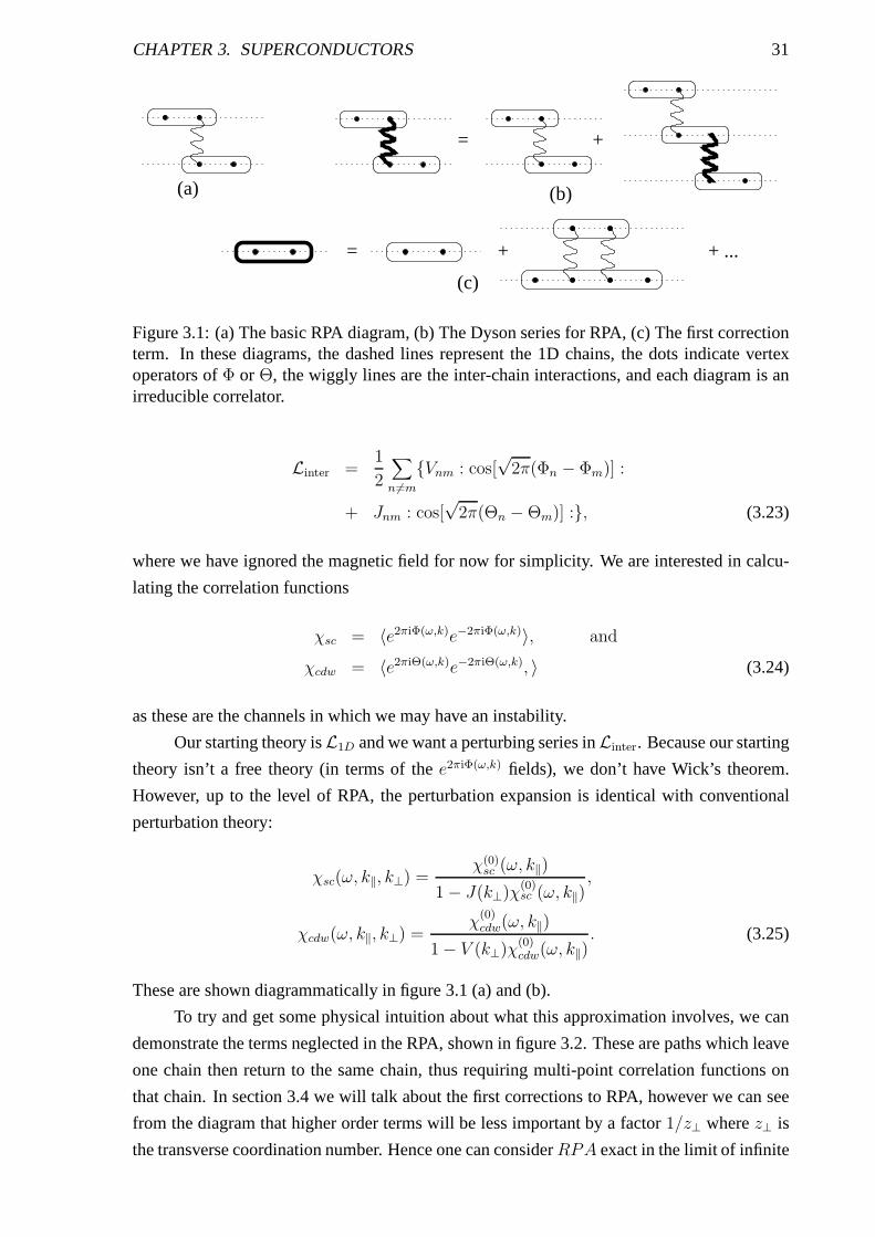
Figure 3.1: (a) The basic RPA diagram, (b) The Dyson series for RPA, (c) The first correctionterm. In these diagrams, the dashed lines represent the 1D chains, the dots indicate vertexoperators ofΦ or Θ, the wiggly lines are the inter-chain interactions, and each diagram is anirreducible correlator.
Linter =1
2
∑
n 6=m{Vnm : cos[
√2π(Φn − Φm)] :
+ Jnm : cos[√
2π(Θn − Θm)] :}, (3.23)
where we have ignored the magnetic field for now for simplicity. We are interested in calcu-
lating the correlation functions
χsc = 〈e2πiΦ(ω,k)e−2πiΦ(ω,k)〉, and
χcdw = 〈e2πiΘ(ω,k)e−2πiΘ(ω,k), 〉 (3.24)
as these are the channels in which we may have an instability.
Our starting theory isL1D and we want a perturbing series inLinter. Because our starting
theory isn’t a free theory (in terms of thee2πiΦ(ω,k) fields), we don’t have Wick’s theorem.
However, up to the level of RPA, the perturbation expansion is identical with conventional
perturbation theory:
χsc(ω, k‖, k⊥) =χ(0)sc (ω, k‖)
1 − J(k⊥)χ(0)sc (ω, k‖)
,
χcdw(ω, k‖, k⊥) =χ
(0)cdw(ω, k‖)
1 − V (k⊥)χ(0)cdw(ω, k‖)
. (3.25)
These are shown diagrammatically in figure 3.1 (a) and (b).
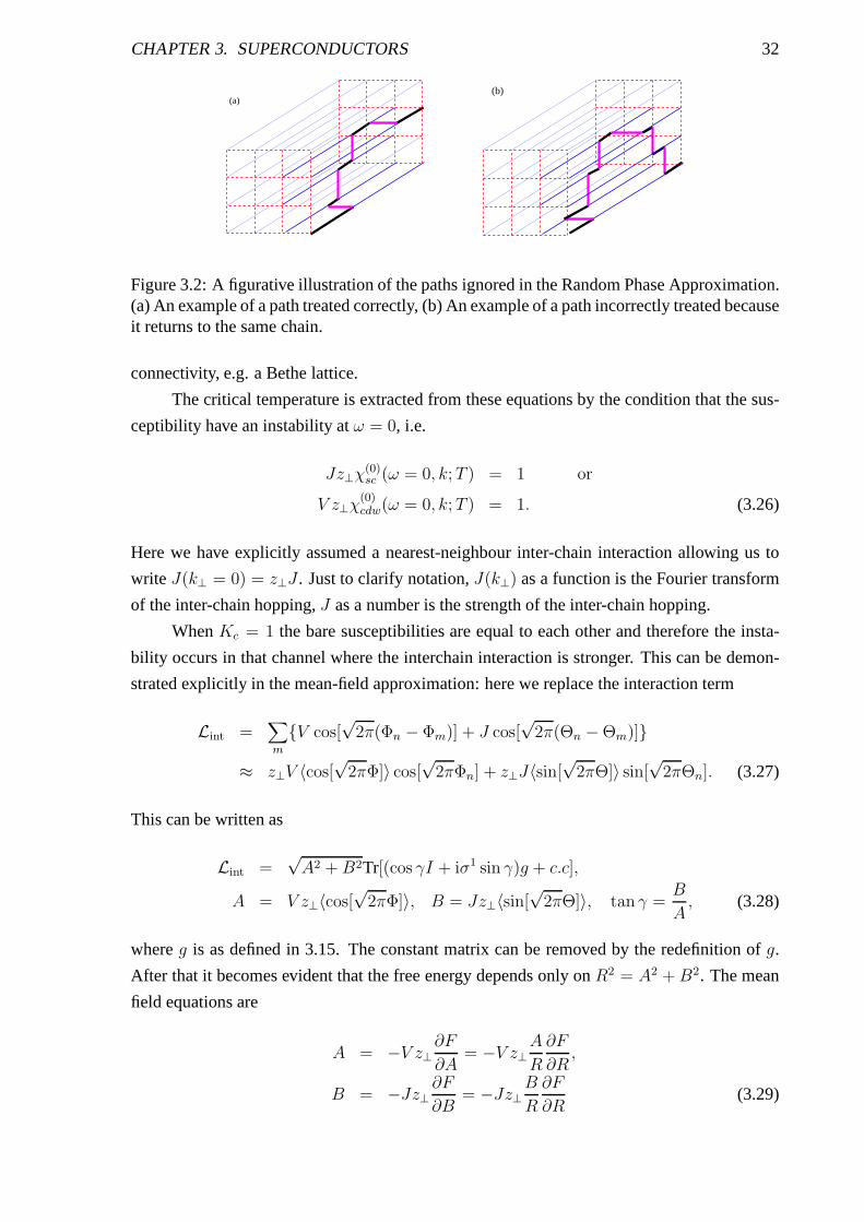
To try and get some physical intuition about what this approximation involves, we can
demonstrate the terms neglected in the RPA, shown in figure 3.2. These are paths which leave
one chain then return to the same chain, thus requiring multi-point correlation functions on
that chain. In section 3.4 we will talk about the first corrections to RPA, however we can see
from the diagram that higher order terms will be less important by a factor1/z⊥ wherez⊥ is
the transverse coordination number. Hence one can considerRPA exact in the limit of infinite
CHAPTER 3. SUPERCONDUCTORS 32
(a)(b)
Figure 3.2: A figurative illustration of the paths ignored inthe Random Phase Approximation.(a) An example of a path treated correctly, (b) An example of apath incorrectly treated becauseit returns to the same chain.
connectivity, e.g. a Bethe lattice.
The critical temperature is extracted from these equationsby the condition that the sus-
ceptibility have an instability atω = 0, i.e.
Jz⊥χ(0)sc (ω = 0, k;T ) = 1 or
V z⊥χ(0)cdw(ω = 0, k;T ) = 1. (3.26)
Here we have explicitly assumed a nearest-neighbour inter-chain interaction allowing us to
write J(k⊥ = 0) = z⊥J . Just to clarify notation,J(k⊥) as a function is the Fourier transform
of the inter-chain hopping,J as a number is the strength of the inter-chain hopping.
WhenKc = 1 the bare susceptibilities are equal to each other and therefore the insta-
bility occurs in that channel where the interchain interaction is stronger. This can be demon-
strated explicitly in the mean-field approximation: here wereplace the interaction term
Lint =∑
m
{V cos[√
2π(Φn − Φm)] + J cos[√
2π(Θn − Θm)]}
≈ z⊥V 〈cos[√
2πΦ]〉 cos[√
2πΦn] + z⊥J〈sin[√
2πΘ]〉 sin[√
2πΘn]. (3.27)
This can be written as
Lint =√A2 +B2Tr[(cos γI + iσ1 sin γ)g + c.c],
A = V z⊥〈cos[√
2πΦ]〉, B = Jz⊥〈sin[√
2πΘ]〉, tan γ =B
A, (3.28)
whereg is as defined in 3.15. The constant matrix can be removed by theredefinition ofg.
After that it becomes evident that the free energy depends only onR2 = A2 +B2. The mean
field equations are
A = −V z⊥∂F
∂A= −V z⊥
A
R
∂F
∂R,
B = −Jz⊥∂F
∂B= −Jz⊥
B
R
∂F
∂R(3.29)
CHAPTER 3. SUPERCONDUCTORS 33
From this it is clear that the only case where bothA andB are simultaneously non-zero is
V = J .
If Kc 6= 1, the instability still occurs in the stronger channel, although this now depends
not only on the values ofV andJ but also onKc and∆s, the crossover point being
(
t2
∆s
vc
) 1
2−1/2Kc
∼(
V
vc
)
1
2−Kc/2
. (3.30)
For definiteness let us assume that the instability occurs inthe superconducting channel
which is the most likely case forKc > 1. Note that the duality property of the effective
Lagrangian (3.14) underK → 1/K, V ↔ J, Θ ↔ Φ means that all of the results in this and
the next section are identical for the CDW channel.
In a Tomonaga-Luttinger liquid with the ultraviolet cut-off ∆s the static susceptibility
for the operator with scaling dimensiond was given in section 2.3:
χ(0)(k) =2
∆2s
sin πd(
2πT
∆s
)−2+2d
Γ2(1 − d)
∣
∣
∣
∣
∣
Γ(d/2 + ivck/4πT )
Γ(1 − d/2 + ivck/4πT )
∣
∣
∣
∣
∣
2
. (3.31)
In the absence of a magnetic field, the structure ofχ means that the instability will occur at
k = 0.
3.3.3 Zero magnetic field; the critical temperature
Substituting 3.31 withk = 0 into equation 3.25 we obtain
Tc =∆s
2π
(
2Jz⊥∆s
sin πdΓ2(d/2)Γ2(1 − d)
Γ2(1 − d/2)
) 1
2−2d
. (3.32)
Below the transition temperature the long-wavelength fluctuations of superconducting
order parameter are three-dimensional. The amplitude fluctuations are however mostly one-
dimensional and their spectral weight is concentrated above a certain energy which plays the
role of a pseudo-gap. The zero temperature value of the pseudo-gap can be found from the
mean-field theory combined with the exact results for the sine-Gordon model. In this approach
one approximates the inter-chain interaction
J∑
<nm>
cos[√
2πK−1c (Θn − Θm)], (3.33)
by the one-dimensional (i.e. no chain index) term:
2µ cos[√
2πK−1c Θ], (3.34)
where
2µ = Jz⊥∆s〈cos[√
2πK−1c Θ]〉. (3.35)
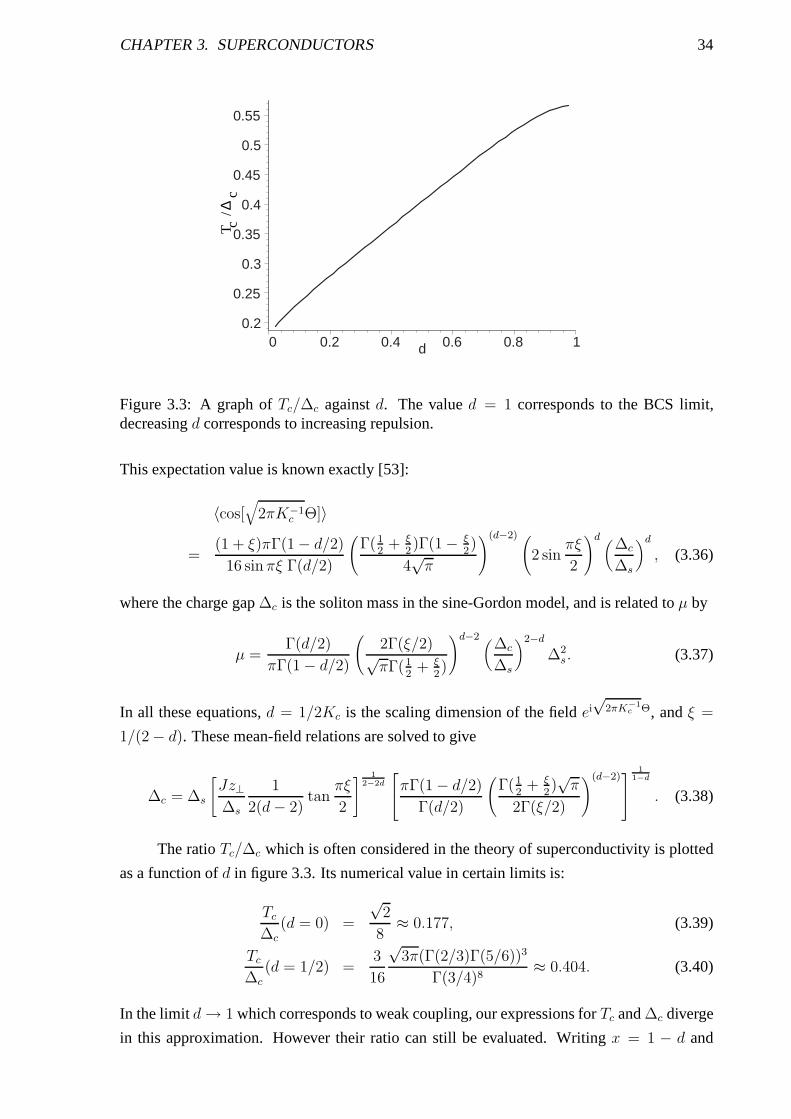
CHAPTER 3. SUPERCONDUCTORS 34
0.2
0.25
0.3
0.35
0.4
0.45
0.5
0.55
0 0.2 0.4 0.6 0.8 1d
T c/
c∆
Figure 3.3: A graph ofTc/∆c againstd. The valued = 1 corresponds to the BCS limit,decreasingd corresponds to increasing repulsion.
This expectation value is known exactly [53]:
〈cos[√
2πK−1c Θ]〉
=(1 + ξ)πΓ(1 − d/2)
16 sin πξ Γ(d/2)
(
Γ(12
+ ξ2)Γ(1 − ξ
2)
4√π
)(d−2) (
2 sinπξ
2
)d (∆c
∆s
)d
, (3.36)
where the charge gap∆c is the soliton mass in the sine-Gordon model, and is related to µ by
µ =Γ(d/2)
πΓ(1 − d/2)
(
2Γ(ξ/2)√πΓ(1
2+ ξ
2)
)d−2 (∆c
∆s
)2−d∆2s. (3.37)
In all these equations,d = 1/2Kc is the scaling dimension of the fieldei√
2πK−1c Θ, andξ =
1/(2 − d). These mean-field relations are solved to give
∆c = ∆s
[
Jz⊥∆s
1
2(d− 2)tan
πξ
2
]1
2−2d
πΓ(1 − d/2)
Γ(d/2)
(
Γ(12
+ ξ2)√π
2Γ(ξ/2)
)(d−2)
1
1−d
. (3.38)
The ratioTc/∆c which is often considered in the theory of superconductivity is plotted
as a function ofd in figure 3.3. Its numerical value in certain limits is:
Tc∆c
(d = 0) =
√2
8≈ 0.177, (3.39)
Tc∆c
(d = 1/2) =3
16
√3π(Γ(2/3)Γ(5/6))3
Γ(3/4)8≈ 0.404. (3.40)
In the limitd→ 1 which corresponds to weak coupling, our expressions forTc and∆c diverge
in this approximation. However their ratio can still be evaluated. Writingx = 1 − d and
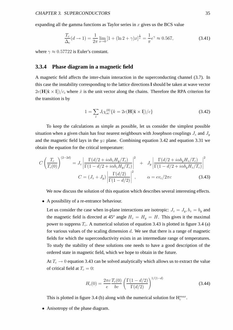
CHAPTER 3. SUPERCONDUCTORS 35
expanding all the gamma functions as Taylor series inx gives us the BCS value
Tc∆c
(d→ 1) =1
2πlimx→0
[1 + (ln 2 + γ)x]1
x =1
πeγ ≈ 0.567, (3.41)
whereγ ≈ 0.57722 is Euler’s constant.
3.3.4 Phase diagram in a magnetic field
A magnetic field affects the inter-chain interaction in the superconducting channel (3.7). In
this case the instability corresponding to the lattice directionsl should be taken at wave vector
2e(H[x× l])/c, wherex is the unit vector along the chains. Therefore the RPA criterion for
the transition is by
1 =∑
l
Jlχ(0)sc {k = 2e(H[x× l])/c} (3.42)
To keep the calculations as simple as possible, let us consider the simplest possible
situation when a given chain has four nearest neighbours with Josephson couplingsJz andJyand the magnetic field lays in theyz plane. Combining equation 3.42 and equation 3.31 we
obtain the equation for the critical temperature:
C
(
TcTc(0)
)(2−2d)
= Jz
∣
∣
∣
∣
∣
Γ(d/2 + iαbzHy/Tc)
Γ(1 − d/2 + iαbzHy/Tc)
∣
∣
∣
∣
∣
2
+ Jy
∣
∣
∣
∣
∣
Γ(d/2 + iαbyHz/Tc)
Γ(1 − d/2 + iαbyHz/Tc)
∣
∣
∣
∣
∣
2
C = (Jz + Jy)
∣
∣
∣
∣
∣
Γ(d/2)
Γ(1 − d/2)
∣
∣
∣
∣
∣
2
, α = evc/2πc (3.43)
We now discuss the solution of this equation which describesseveral interesting effects.
• A possibility of a re-entrance behaviour.
Let us consider the case when in-plane interactions are isotropic: Jz = Jy, bz = by and
the magnetic field is directed at 45o angleHz = Hy = H. This gives it the maximal
power to suppressTc. A numerical solution of equation 3.43 is plotted in figure 3.4 (a)
for various values of the scaling dimensiond. We see that there is a range of magnetic
fields for which the superconductivity exists in an intermediate range of temperatures.
To study the stability of these solutions one needs to have a good description of the
ordered state in magnetic field, which we hope to obtain in thefuture.
At Tc → 0 equation 3.43 can be solved analytically which allows us to extract the value
of critical field atTc = 0:
Hc(0) =2πc
e
Tc(0)
bv
(
Γ(1 − d/2)
Γ(d/2)
)1/(1−d)(3.44)
This is plotted in figure 3.4 (b) along with the numerical solution for Hmaxc .
• Anisotropy of the phase diagram.
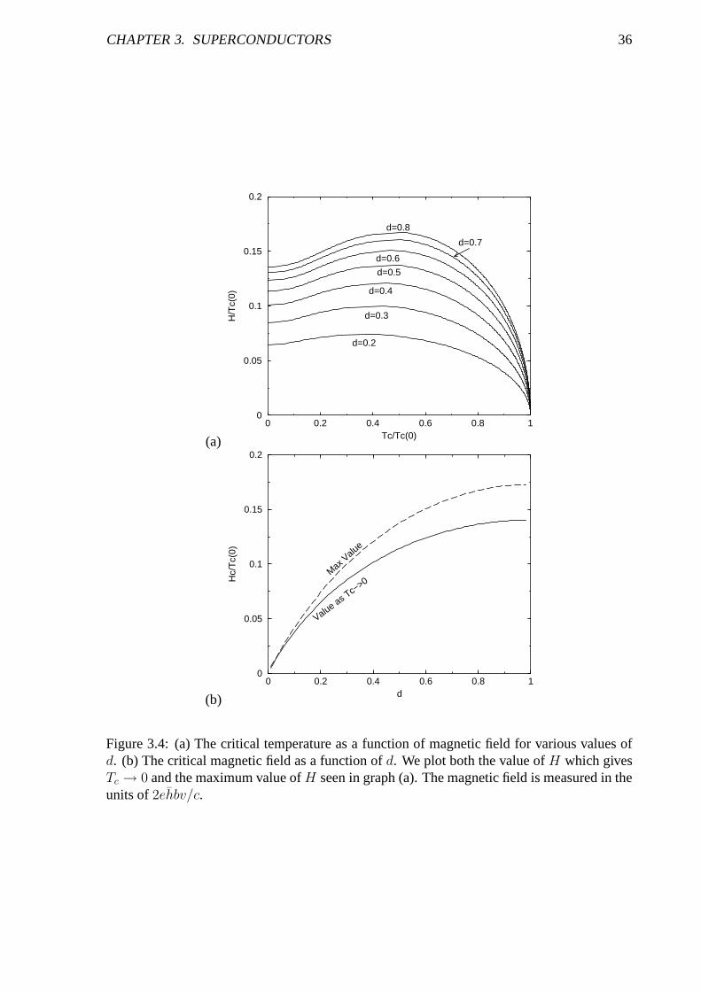
CHAPTER 3. SUPERCONDUCTORS 36
(a)
0 0.2 0.4 0.6 0.8 1Tc/Tc(0)
0
0.05
0.1
0.15
0.2
H/T
c(0)
d=0.2
d=0.3
d=0.4
d=0.5
d=0.6
d=0.7
d=0.8
(b)
0 0.2 0.4 0.6 0.8 1d
0
0.05
0.1
0.15
0.2
Hc/
Tc(
0)
Max V
alue
Value as Tc−
>0
Figure 3.4: (a) The critical temperature as a function of magnetic field for various values ofd. (b) The critical magnetic field as a function ofd. We plot both the value ofH which givesTc → 0 and the maximum value ofH seen in graph (a). The magnetic field is measured in theunits of2ehbv/c.
CHAPTER 3. SUPERCONDUCTORS 37
H
H
x
y
Figure 3.5: Angular dependence of the critical magnetic field. This is plotted ford = 1/2.The graph is qualitatively similar for other values ofd. In actual fact, the system will be drivento a CDW ground state before the SC transition temperature drops to zero - see the text.
Another prediction following from equation 3.43 is an anisotropy of the phase diagram.
This can be illustrated by an analytical solution of the critical field for whichTc → 0.
SettingTc → 0 in equation 3.43 we find
Jz(αHybz)2(1−d) +
Jy(αHzby)2(1−d) =
C
[Tc(0)]2(1−d), (3.45)
whereα is an unimportant constant factor. This is plotted in figure 3.5. We must be
careful to remember however that this is a first order mean field calculation, and further
corrections will give a critical flux in all directions, evenwhen the field is pointing
directly along one of the crystal axis.
• SC-CDW transition.
The above calculations are all calculated assuming we are ina parameter range such that
the ground state atH = 0 is superconducting. However, as we increase the magnetic
field and thus reduce the SC transition temperature, we eventually get to a regime where
TCDW > TSC as the CDW instability is not affected by the magnetic field. At this point
which can happen either by increasing magnetic field (figure 3.4) or by changing the
angle of the magnetic field (figure 3.5), we get a first order transition from a supercon-
ducting to a CDW state. The latter would be a very unusual effect to observe in a real
material.
3.4 Corrections to RPA
The analysis of the previous sections was based on the RPA. Inrealistic situations the number
of nearest neighbours is never large, so it is important to check how robust the RPA is. We
will calculate corrections to RPA in the simplest case case of zero magnetic field. We shall
also restrict ourselves toKc = 1 (d = 1/2 for both interactions).
The basic RPA calculation involves only the stronger of the two interactions - for clarity
let us again take this to be J. However as we mentioned before we would expect the presence of
CHAPTER 3. SUPERCONDUCTORS 38
the other competing interaction of the same scaling dimension to also play a role. In particular
we expect there to be a mode with a gap ofJ − V , seen in equation 3.22 and in the two chain
model. This will be very important around the pointV = J as it will become massless thereby
increasing fluctuations and decreasing the transition temperature. This can be investigated by
looking at the first correction to the RPA formula - figure 3.1(c).
In terms of the fieldsφ andθ, this diagram can be expressed as
δχ = V 2z⊥[
〈ei√
2πΘ(a)ei√
2πΦ(1)e−i√
2πΦ(2)e−i√
2πΘ(b)〉 − 〈ei√
2πΘ(a)e−i√
2πΘ(b)〉〈ei√
2πΦ(1)e−i√
2πΦ(2)〉]
×〈e−i√
2πΦ(1)ei√
2πΦ(2)〉+ J2z⊥
[
〈ei√
2πΘ(a)ei√
2πΘ(1)e−i√
2πΘ(2)e−i√
2πΘ(b)〉 − 〈ei√
2πΘ(a)e−i√
2πΘ(b)〉〈ei√
2πΘ(1)e−i√
2πΘ(2)〉]
× 〈e−i√
2πΘ(1)ei√
2πΘ(2)〉, (3.46)
wherea,b are the start and end points and1,2 are the intermediate points to be integrated over.
Substituting in the expectation values from equation 2.4 and integrating gives the revised RPA
equation for the transition temperature:
1 =Jz⊥Tc
[
AJ0 + AJ1J2z⊥T 2c
+ AV1V 2z⊥T 2c
]
(3.47)
where the coefficients are given by
AJ0 =1
π
∫ π
0dτ∫ ∞
−∞dx
1
| sinh(x+ iτ)| =1
2πB2(1/4, 1/2),
AJ1 =1
π3
∫ π
0dτ1dτ2dτb
∫ ∞
−∞dx1dx2dxb
1
| sinh(xb + iτb)|1
| sinh(x12 + iτ12)|2
×[
| sinh(x1 + iτ1)|| sinh(xb2 + iτb2)|| sinh(x2 + iτ2)|| sinh(xb1 + iτb1)|
− 1
]
,
AV1 =1
π3
∫ π
0dτ1dτ2dτb
∫ ∞
−∞dx1dx2dxb
1
| sinh(xb + iτb)|1
| sinh(x12 + iτ12)|2
×
(
sinh(x1 + iτ1) sinh(x2 − iτ2) sinh(xb2 + iτb2) sinh(xb1 − iτb1)
sinh(x1 − iτ1) sinh(x2 + iτ2) sinh(xb2 − iτb2) sinh(xb1 + iτb1)
)1/2
− 1
(3.48)
with x12 = x2 − x1 and so on.B(x, y) = Γ(x)Γ(y)/Γ(x+ y) is a Beta function.
The integrals are evaluated numerically by Monte-Carlo techniques [54] with values
calculated over finite volumes then scaled to infinity. The results are
AJ0 = 4.377,
AJ1 = 34.81 ± 0.02,
AV1 = −33.01 ± 0.02. (3.49)
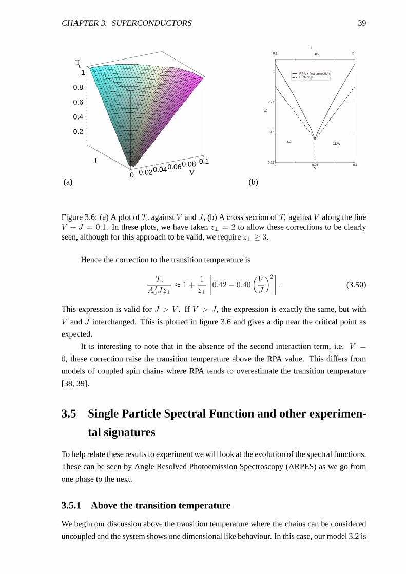
CHAPTER 3. SUPERCONDUCTORS 39
(a)0 0.020.040.060.08 0.1
0.2
0.4
0.6
0.8
1Tc
V
J
(b)
0 0.05 0.1V
0.25
0.5
0.75
1
Tc
RPA + first correctionRPA only
00.050.1
J
SCCDW
Figure 3.6: (a) A plot ofTc againstV andJ , (b) A cross section ofTc againstV along the lineV + J = 0.1. In these plots, we have takenz⊥ = 2 to allow these corrections to be clearlyseen, although for this approach to be valid, we requirez⊥ ≥ 3.
Hence the correction to the transition temperature is
TcAJ0Jz⊥
≈ 1 +1
z⊥
[
0.42 − 0.40(
V
J
)2]
. (3.50)
This expression is valid forJ > V . If V > J , the expression is exactly the same, but with
V andJ interchanged. This is plotted in figure 3.6 and gives a dip near the critical point as
expected.
It is interesting to note that in the absence of the second interaction term, i.e.V =
0, these correction raise the transition temperature above the RPA value. This differs from
models of coupled spin chains where RPA tends to overestimate the transition temperature
[38, 39].
3.5 Single Particle Spectral Function and other experimen-
tal signatures
To help relate these results to experiment we will look at theevolution of the spectral functions.
These can be seen by Angle Resolved Photoemission Spectroscopy (ARPES) as we go from
one phase to the next.
3.5.1 Above the transition temperature
We begin our discussion above the transition temperature where the chains can be considered
uncoupled and the system shows one dimensional like behaviour. In this case, our model 3.2 is
CHAPTER 3. SUPERCONDUCTORS 40
simply a Luther-Emery liquid [19]. The correlation functions in the spin-sector can be written
as a form-factor expansion [20] but results are only known for T = 0, and the first correction
for T << ∆s in [55]. Although finite temperature results are known in thecharge sector, the
convolution of this with the spin sector does not admit to easy analytical analysis. However, at
the Luther-Emery point,Kc = 1/2 (see section 2.1.4) where the spin sector can be rewritten in
terms of free fermions, a number of analytic results can be recovered. Details of this are found
in [56] and [43], here we limit ourselves here to a discussionof the overall gross features.
At the Luther-Emery pointKs = 1/2, the field operators in the refermionised form
can be thought of as spin soliton creation and annihilation operators. Hence the spin part of
the spectral function can be written as the sum of a coherent one spin soliton part and an
incoherent multi-soliton piece
As(k, ω) = Zs(k)δ[ω + Es(k)] +G(multi)s (k, ω) (3.51)
where the multi-soliton piece atT = 0 is zero below the threshold energyω3 = 3Es(k/3). As
the solitons can be written as free fermions, their spectrumis
Es(k) =√
∆2s + (vsk)2. (3.52)
Away from the Luther-Emery point forKs < 1/2, soliton-antisoliton bound-states form which
will shift the threshold energy slightly.
The convolution with the charge sector (Ec(k) = vc|k|) gives the result
A(k, ω;T ) =c2
π3
λ2T
vc
(
a0
λT
)2θc+1
2
(
2vsa0∆s
)
3
8
×∫
dq
[
1 − vs(k − q)
Es(k − q)
]
hθc+1
2
[
ω + Es(k − q) + vcq
2πT
]
× hθc
[
ω + Es(k − q) − vcq
2πT
]
+ . . . , (3.53)
where the. . . refer to the 3 spin soliton and higher contributions andλT = vc/πT is the
thermal length. In this expression,
hθ(k) = Re
[
(2i)θB
(
θ − ik
2, 1 − θ
)]
. (3.54)
Although this is calculated only at the Luther-Emery point,it is expected that the basic features
remain the same throughout the spin-gap region (and furthermore in the regionTc < T <
∆s, even when the spin sector is far more complicated). The shape of the spectral functions
is plotted in the way typical in ARPES as various Energy Distribution Curves (EDC’s) at
constant momenta and momentum distribution curves (MDC’s)at constant energy in figure
3.7, showing the effects of a spin-gap.
We see that in the MDC at the Fermi-level, it is hard to distinguish between this sys-
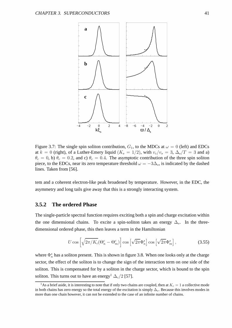
CHAPTER 3. SUPERCONDUCTORS 41
−4 −2 0 2 4kξs
−8 −6 −4 −2 0 2ω / ∆s
a
b
c
Figure 3.7: The single spin soliton contribution,G1, to the MDCs atω = 0 (left) and EDCsat k = 0 (right), of a Luther-Emery liquid(Ks = 1/2), with vc/vs = 3, ∆s/T = 3 and a)θc = 0, b) θc = 0.2, and c)θc = 0.4. The asymptotic contribution of the three spin solitonpiece, to the EDCs, near its zero temperature thresholdω = −3∆s, is indicated by the dashedlines. Taken from [56].
tem and a coherent electron-like peak broadened by temperature. However, in the EDC, the
asymmetry and long tails give away that this is a strongly interacting system.
3.5.2 The ordered Phase
The single-particle spectral function requires exciting both a spin and charge excitation within
the one dimensional chains. To excite a spin-soliton takes an energy∆s. In the three-
dimensional ordered phase, this then leaves a term in the Hamiltonian
U cos[
√
2π/Kc(Θcn − Θc
m)]
cos[√
2πΦsn
]
cos[√
2πΦsm
]
, (3.55)
whereΦsn has a soliton present. This is shown in figure 3.8. When one looks only at the charge
sector, the effect of the soliton is to change the sign of the interaction term on one side of the
soliton. This is compensated for by a soliton in the charge sector, which is bound to the spin
soliton. This turns out to have an energy1 ∆c/2 [57].
1As a brief aside, it is interesting to note that if only two chains are coupled, then atKc = 1 a collective modein both chains has zero energy so the total energy of the excitation is simply∆s. Because this involves modes inmore than one chain however, it can not be extended to the caseof an infinite number of chains.
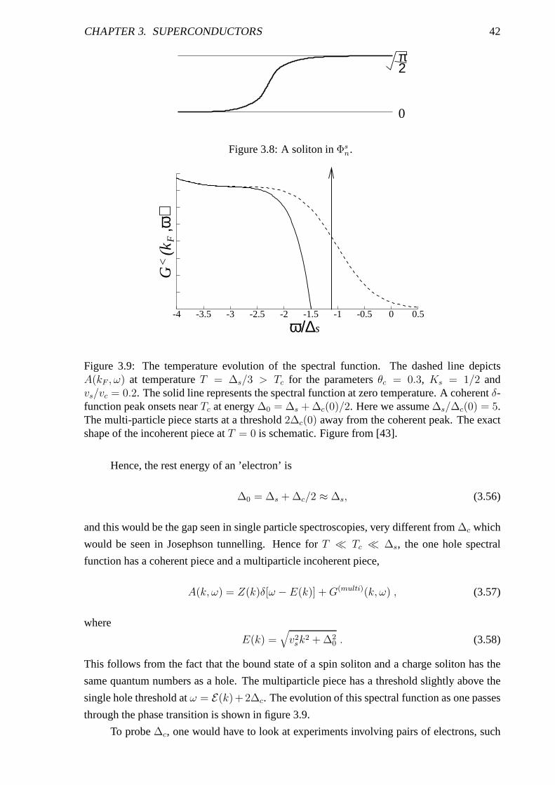
CHAPTER 3. SUPERCONDUCTORS 42
π
0
2
Figure 3.8: A soliton inΦsn.
(k<
G
ω/∆s
F,ω
)
-4 -3.5 -3 -2.5 -2 -1.5 -1 -0.5 0 0.5
Figure 3.9: The temperature evolution of the spectral function. The dashed line depictsA(kF , ω) at temperatureT = ∆s/3 > Tc for the parametersθc = 0.3, Ks = 1/2 andvs/vc = 0.2. The solid line represents the spectral function at zero temperature. A coherentδ-function peak onsets nearTc at energy∆0 = ∆s + ∆c(0)/2. Here we assume∆s/∆c(0) = 5.The multi-particle piece starts at a threshold2∆c(0) away from the coherent peak. The exactshape of the incoherent piece atT = 0 is schematic. Figure from [43].
Hence, the rest energy of an ’electron’ is
∆0 = ∆s + ∆c/2 ≈ ∆s, (3.56)
and this would be the gap seen in single particle spectroscopies, very different from∆c which
would be seen in Josephson tunnelling. Hence forT ≪ Tc ≪ ∆s, the one hole spectral
function has a coherent piece and a multiparticle incoherent piece,
A(k, ω) = Z(k)δ[ω − E(k)] +G(multi)(k, ω) , (3.57)
where
E(k) =√
v2sk
2 + ∆20 . (3.58)
This follows from the fact that the bound state of a spin soliton and a charge soliton has the
same quantum numbers as a hole. The multiparticle piece has athreshold slightly above the
single hole threshold atω = E(k)+2∆c. The evolution of this spectral function as one passes
through the phase transition is shown in figure 3.9.
To probe∆c, one would have to look at experiments involving pairs of electrons, such
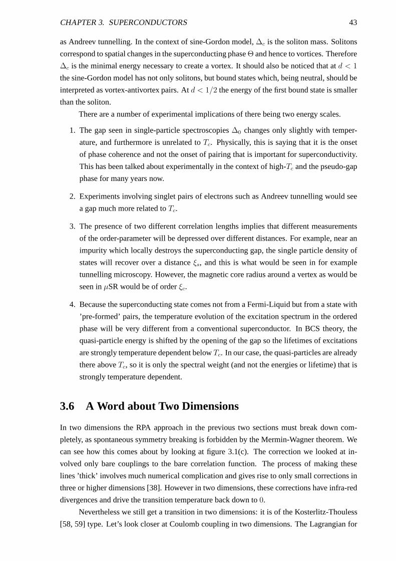
CHAPTER 3. SUPERCONDUCTORS 43
as Andreev tunnelling. In the context of sine-Gordon model,∆c is the soliton mass. Solitons
correspond to spatial changes in the superconducting phaseΘ and hence to vortices. Therefore
∆c is the minimal energy necessary to create a vortex. It shouldalso be noticed that atd < 1
the sine-Gordon model has not only solitons, but bound states which, being neutral, should be
interpreted as vortex-antivortex pairs. Atd < 1/2 the energy of the first bound state is smaller
than the soliton.
There are a number of experimental implications of there being two energy scales.
1. The gap seen in single-particle spectroscopies∆0 changes only slightly with temper-
ature, and furthermore is unrelated toTc. Physically, this is saying that it is the onset
of phase coherence and not the onset of pairing that is important for superconductivity.
This has been talked about experimentally in the context of high-Tc and the pseudo-gap
phase for many years now.
2. Experiments involving singlet pairs of electrons such asAndreev tunnelling would see
a gap much more related toTc.
3. The presence of two different correlation lengths implies that different measurements
of the order-parameter will be depressed over different distances. For example, near an
impurity which locally destroys the superconducting gap, the single particle density of
states will recover over a distanceξs, and this is what would be seen in for example
tunnelling microscopy. However, the magnetic core radius around a vertex as would be
seen inµSR would be of orderξc.
4. Because the superconducting state comes not from a Fermi-Liquid but from a state with
’pre-formed’ pairs, the temperature evolution of the excitation spectrum in the ordered
phase will be very different from a conventional superconductor. In BCS theory, the
quasi-particle energy is shifted by the opening of the gap sothe lifetimes of excitations
are strongly temperature dependent belowTc. In our case, the quasi-particles are already
there aboveTc, so it is only the spectral weight (and not the energies or lifetime) that is
strongly temperature dependent.
3.6 A Word about Two Dimensions
In two dimensions the RPA approach in the previous two sections must break down com-
pletely, as spontaneous symmetry breaking is forbidden by the Mermin-Wagner theorem. We
can see how this comes about by looking at figure 3.1(c). The correction we looked at in-
volved only bare couplings to the bare correlation function. The process of making these
lines ’thick’ involves much numerical complication and gives rise to only small corrections in
three or higher dimensions [38]. However in two dimensions,these corrections have infra-red
divergences and drive the transition temperature back downto 0.
Nevertheless we still get a transition in two dimensions: itis of the Kosterlitz-Thouless
[58, 59] type. Let’s look closer at Coulomb coupling in two dimensions. The Lagrangian for
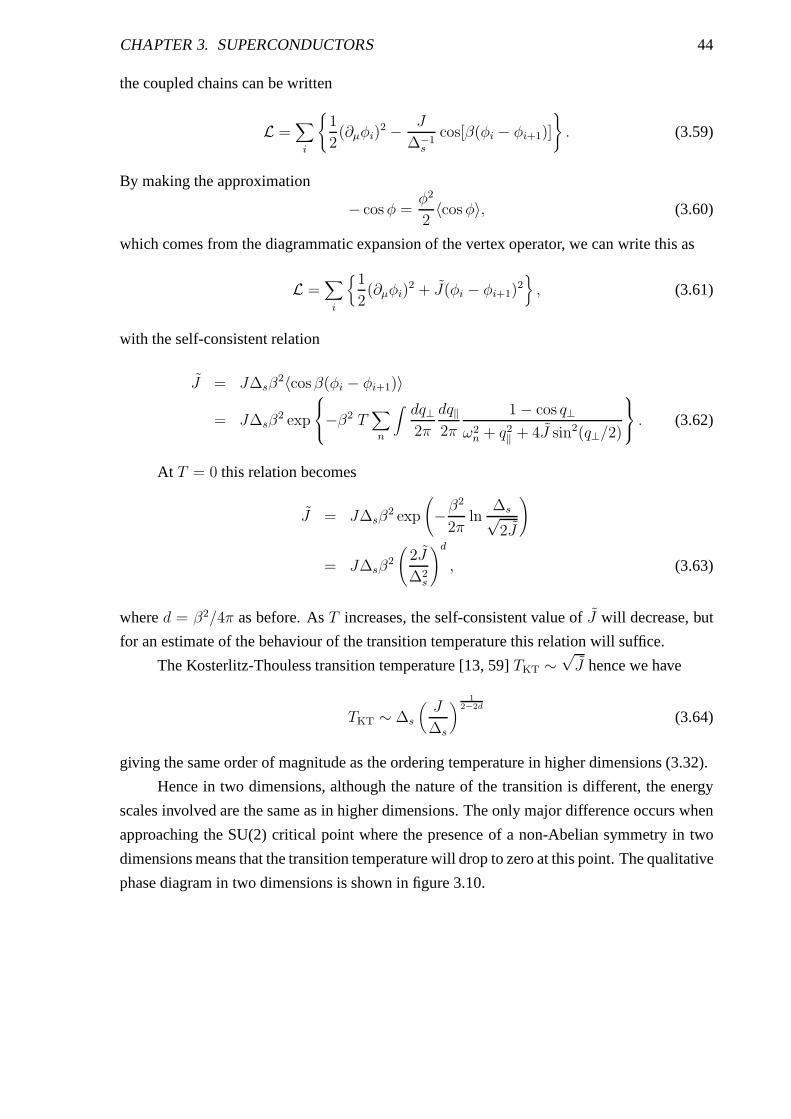
CHAPTER 3. SUPERCONDUCTORS 44
the coupled chains can be written
L =∑
i
{
1
2(∂µφi)
2 − J
∆−1s
cos[β(φi − φi+1)]
}
. (3.59)
By making the approximation
− cosφ =φ2
2〈cosφ〉, (3.60)
which comes from the diagrammatic expansion of the vertex operator, we can write this as
L =∑
i
{
1
2(∂µφi)
2 + J(φi − φi+1)2}
, (3.61)
with the self-consistent relation
J = J∆sβ2〈cosβ(φi − φi+1)〉
= J∆sβ2 exp
−β2 T∑
n
∫
dq⊥2π
dq‖2π
1 − cos q⊥
ω2n + q2
‖ + 4J sin2(q⊥/2)
. (3.62)
At T = 0 this relation becomes
J = J∆sβ2 exp
(
−β2
2πln
∆s√2J
)
= J∆sβ2
(
2J
∆2s
)d
, (3.63)
whered = β2/4π as before. AsT increases, the self-consistent value ofJ will decrease, but
for an estimate of the behaviour of the transition temperature this relation will suffice.
The Kosterlitz-Thouless transition temperature [13, 59]TKT ∼√J hence we have
TKT ∼ ∆s
(
J
∆s
)
1
2−2d
(3.64)
giving the same order of magnitude as the ordering temperature in higher dimensions (3.32).
Hence in two dimensions, although the nature of the transition is different, the energy
scales involved are the same as in higher dimensions. The only major difference occurs when
approaching the SU(2) critical point where the presence of anon-Abelian symmetry in two
dimensions means that the transition temperature will dropto zero at this point. The qualitative
phase diagram in two dimensions is shown in figure 3.10.
CHAPTER 3. SUPERCONDUCTORS 45
Tc
V/J
SC CDW
Figure 3.10: The modified phase diagram for our model in two dimensions
Figure 3.11: Structure ofSr14Cu24O41 after [60]. The compound consists of alternating planesof copper oxide chains and ladders.
CHAPTER 3. SUPERCONDUCTORS 46
3.7 Example experimental systems
3.7.1 The telephone number compound
The class of materialsSr14−xCaxCu24O41 are built up from alternating layers of weakly cou-
pledCuO2 chains andCu2O3 two-leg ladders. The material shows a spin gap in both of these
one-dimensional units [61] making it a prime candidate for application of our model. Because
our only requirement in the spin-sector was that it was gapped, our theory is still valid even if
the superconductivity originates from the ladders.
Forx ≥ 11.5, these materials show superconductivity under pressure [62, 63] and NMR
studies [61] also indicate possible charge ordering at low temperature and ambient pressure.
Recent measurements of the electrodynamic response [64] have confirmed the presence of
CDW in this class of compounds. One of the most interesting measurements however is the
DC resistivity [63], which shows a number of features:
• In Sr2.5Ca11.5Cu24O41 below about 4 GPa pressure, the temperature dependence of the
resistivity perpendicular and parallel to the ladders is different. This indicates that differ-
ent mechanisms are governing the transport in these two directions, consistent with the
spin-gap concept. Above 4 GPa the temperature dependence ofthe resistivity anisotropy
becomes weak, which indicates that single particle hoppingbetween ladders is now
possible, i.e. the spin gap has vanished and we have a crossover to a conventional two-
dimensional metallic behaviour. This is consistent with the pressure dependence of the
spin gap observed in recent NMR experiments [60].
• At sufficiently high temperatures, coherent inter-ladder charge dynamics is also seen.
The temperature where this occurs is consistent with the NMRdeterminations of the
spin gap, so we may conclude that the transport properties ofthis material are indeed
governed by weakly interacting one-dimensional spin-gapped units.
In figure 3.12 a phase diagram of this material is shown [65]. At low calcium doping,
there is charge ordering before spin ordering, so our model is inapplicable. However under
increased levels of calcium doping or pressure, the spin gapis the largest energy scale in the
model meaning that our theory may describe the nature of the transition between the CDW
and the SC phases.
In our model, takingKc ≈ 1 we have
Jeff ∼ (∆s/Λ)t2/∆s,
Veff ∼ (∆s/Λ)V0. (3.65)
The size of the spin gap is reasonably constant as we change calcium doping and pressure,
however under pressure the hoppingt will increase which makes the inter-ladder Josephson
coupling stronger until eventually the material becomes a superconductor instead of having
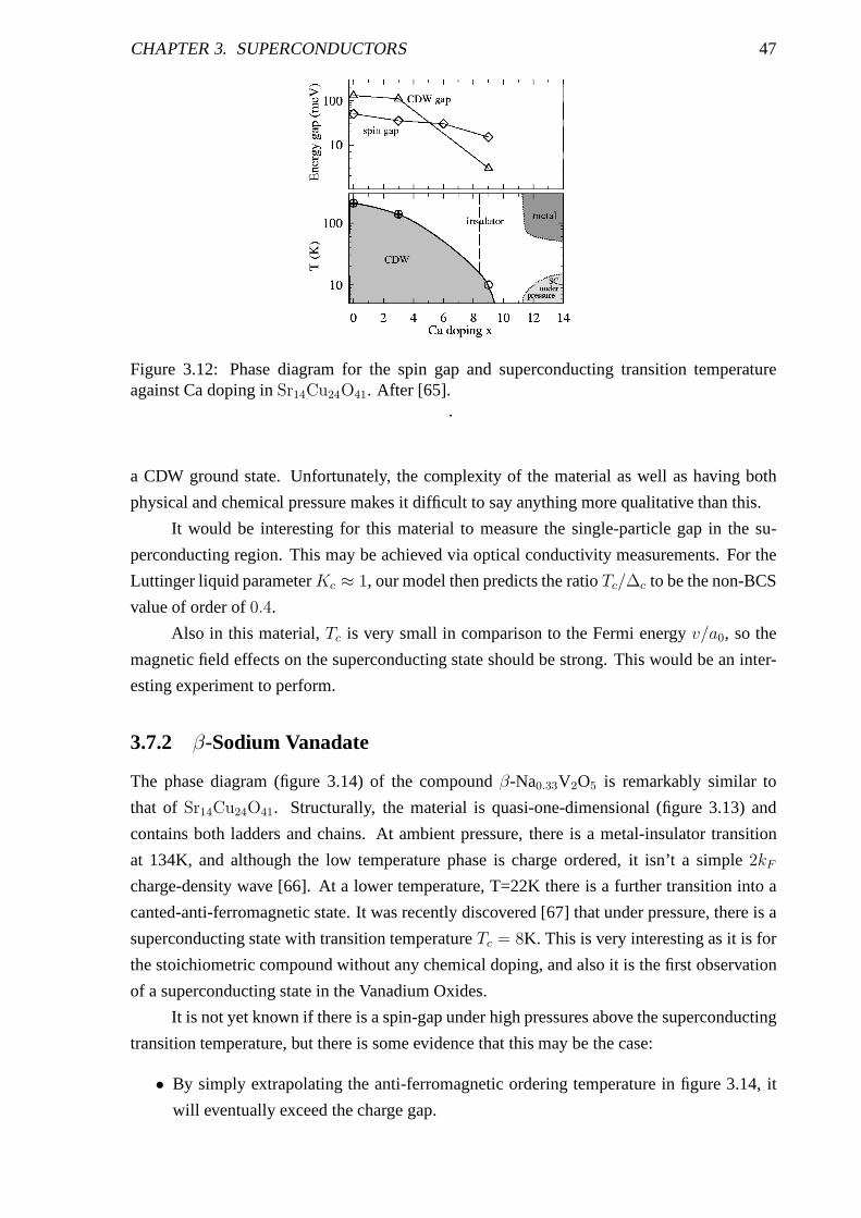
CHAPTER 3. SUPERCONDUCTORS 47
Figure 3.12: Phase diagram for the spin gap and superconducting transition temperatureagainst Ca doping inSr14Cu24O41. After [65].
.
a CDW ground state. Unfortunately, the complexity of the material as well as having both
physical and chemical pressure makes it difficult to say anything more qualitative than this.
It would be interesting for this material to measure the single-particle gap in the su-
perconducting region. This may be achieved via optical conductivity measurements. For the
Luttinger liquid parameterKc ≈ 1, our model then predicts the ratioTc/∆c to be the non-BCS
value of order of0.4.
Also in this material,Tc is very small in comparison to the Fermi energyv/a0, so the
magnetic field effects on the superconducting state should be strong. This would be an inter-
esting experiment to perform.
3.7.2 β-Sodium Vanadate
The phase diagram (figure 3.14) of the compoundβ-Na0.33V2O5 is remarkably similar to
that of Sr14Cu24O41. Structurally, the material is quasi-one-dimensional (figure 3.13) and
contains both ladders and chains. At ambient pressure, there is a metal-insulator transition
at 134K, and although the low temperature phase is charge ordered, it isn’t a simple2kFcharge-density wave [66]. At a lower temperature, T=22K there is a further transition into a
canted-anti-ferromagnetic state. It was recently discovered [67] that under pressure, there is a
superconducting state with transition temperatureTc = 8K. This is very interesting as it is for
the stoichiometric compound without any chemical doping, and also it is the first observation
of a superconducting state in the Vanadium Oxides.
It is not yet known if there is a spin-gap under high pressuresabove the superconducting
transition temperature, but there is some evidence that this may be the case:
• By simply extrapolating the anti-ferromagnetic ordering temperature in figure 3.14, it
will eventually exceed the charge gap.
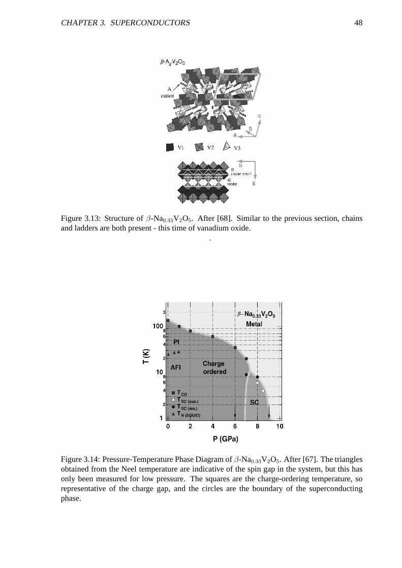
CHAPTER 3. SUPERCONDUCTORS 48
Figure 3.13: Structure ofβ-Na0.33V2O5. After [68]. Similar to the previous section, chainsand ladders are both present - this time of vanadium oxide.
.
Figure 3.14: Pressure-Temperature Phase Diagram ofβ-Na0.33V2O5. After [67]. The trianglesobtained from the Neel temperature are indicative of the spin gap in the system, but this hasonly been measured for low pressure. The squares are the charge-ordering temperature, sorepresentative of the charge gap, and the circles are the boundary of the superconductingphase.

CHAPTER 3. SUPERCONDUCTORS 49
• We additionally have evidence from a number of other materials that the spin gap does
not significantly change with external pressure.
• The similarity between the phase diagrams 3.14 and 3.12 suggests that the supercon-
ducting state could be described by our theory.
This is a very interesting material to study experimentally, and more data should be available
soon.
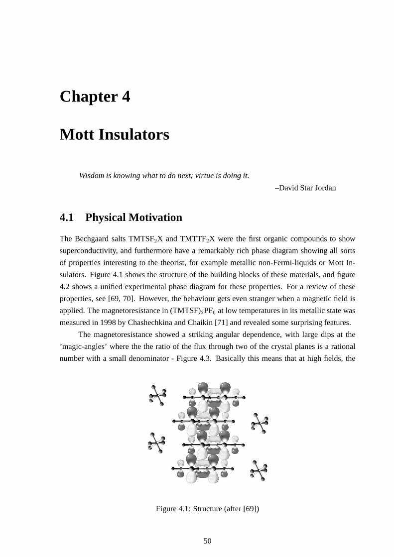
Chapter 4
Mott Insulators
Wisdom is knowing what to do next; virtue is doing it.
–David Star Jordan
4.1 Physical Motivation
The Bechgaard salts TMTSF2X and TMTTF2X were the first organic compounds to show
superconductivity, and furthermore have a remarkably richphase diagram showing all sorts
of properties interesting to the theorist, for example metallic non-Fermi-liquids or Mott In-
sulators. Figure 4.1 shows the structure of the building blocks of these materials, and figure
4.2 shows a unified experimental phase diagram for these properties. For a review of these
properties, see [69, 70]. However, the behaviour gets even stranger when a magnetic field is
applied. The magnetoresistance in (TMTSF)2PF6 at low temperatures in its metallic state was
measured in 1998 by Chashechkina and Chaikin [71] and revealed some surprising features.
The magnetoresistance showed a striking angular dependence, with large dips at the
’magic-angles’ where the the ratio of the flux through two of the crystal planes is a rational
number with a small denominator - Figure 4.3. Basically thismeans that at high fields, the
Figure 4.1: Structure (after [69])
50
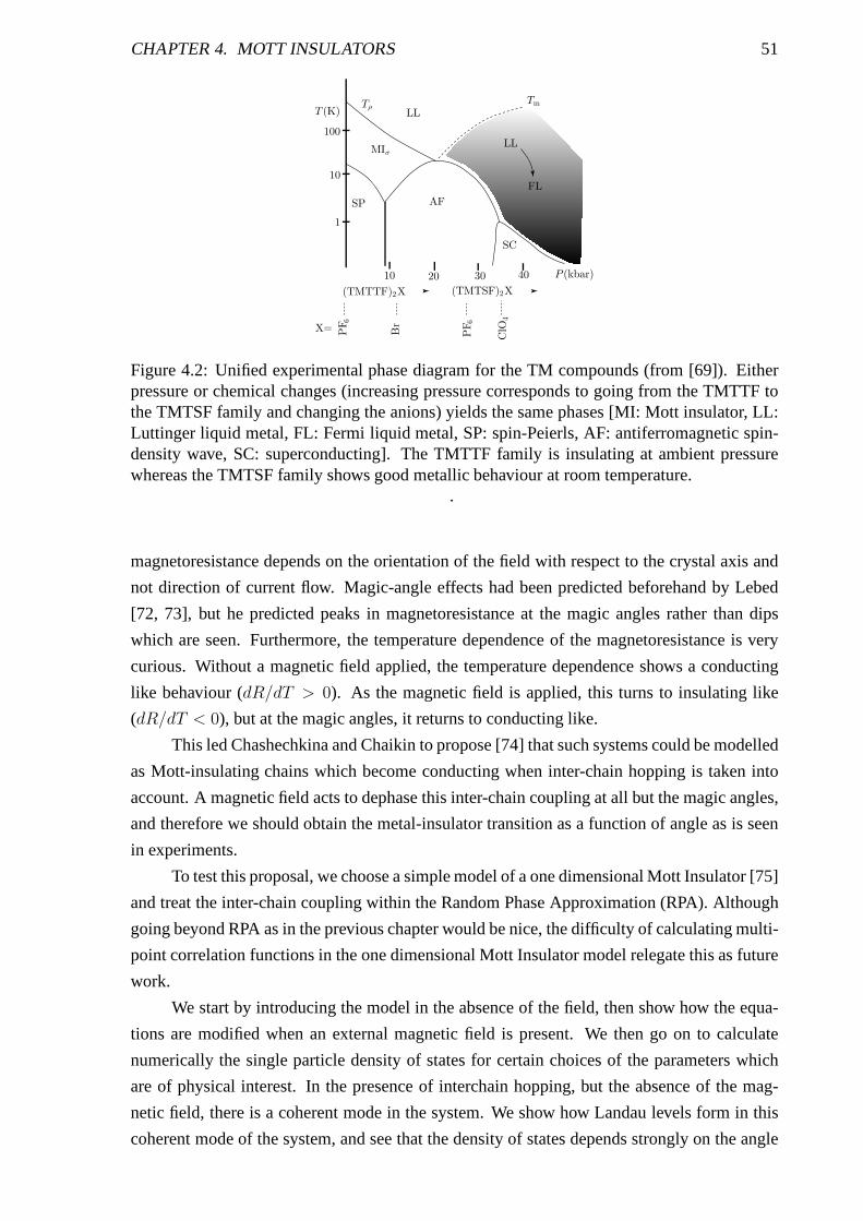
CHAPTER 4. MOTT INSULATORS 51
SP AF
SC
(TMTTF)2X (TMTSF)2X
X= PF 6
Br
ClO
4
10 20 30 40 P (kbar)
10
100
1
T (K)Tρ
PF
6
MIσ
LL
FL
FL
T
LL
m
Figure 4.2: Unified experimental phase diagram for the TM compounds (from [69]). Eitherpressure or chemical changes (increasing pressure corresponds to going from the TMTTF tothe TMTSF family and changing the anions) yields the same phases [MI: Mott insulator, LL:Luttinger liquid metal, FL: Fermi liquid metal, SP: spin-Peierls, AF: antiferromagnetic spin-density wave, SC: superconducting]. The TMTTF family is insulating at ambient pressurewhereas the TMTSF family shows good metallic behaviour at room temperature.
.
magnetoresistance depends on the orientation of the field with respect to the crystal axis and
not direction of current flow. Magic-angle effects had been predicted beforehand by Lebed
[72, 73], but he predicted peaks in magnetoresistance at themagic angles rather than dips
which are seen. Furthermore, the temperature dependence ofthe magnetoresistance is very
curious. Without a magnetic field applied, the temperature dependence shows a conducting
like behaviour (dR/dT > 0). As the magnetic field is applied, this turns to insulating like
(dR/dT < 0), but at the magic angles, it returns to conducting like.
This led Chashechkina and Chaikin to propose [74] that such systems could be modelled
as Mott-insulating chains which become conducting when inter-chain hopping is taken into
account. A magnetic field acts to dephase this inter-chain coupling at all but the magic angles,
and therefore we should obtain the metal-insulator transition as a function of angle as is seen
in experiments.
To test this proposal, we choose a simple model of a one dimensional Mott Insulator [75]
and treat the inter-chain coupling within the Random Phase Approximation (RPA). Although
going beyond RPA as in the previous chapter would be nice, thedifficulty of calculating multi-
point correlation functions in the one dimensional Mott Insulator model relegate this as future
work.
We start by introducing the model in the absence of the field, then show how the equa-
tions are modified when an external magnetic field is present.We then go on to calculate
numerically the single particle density of states for certain choices of the parameters which
are of physical interest. In the presence of interchain hopping, but the absence of the mag-
netic field, there is a coherent mode in the system. We show howLandau levels form in this
coherent mode of the system, and see that the density of states depends strongly on the angle
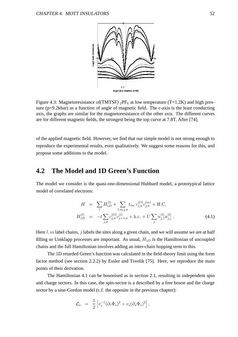
CHAPTER 4. MOTT INSULATORS 52
Figure 4.3: Magnetoresistance of(TMTSF)2PF6 at low temperature (T=1.2K) and high pres-sure (p=9.2kbar) as a function of angle of magnetic field. Thec-axis is the least conductingaxis, the graphs are similar for the magnetoresistance of the other axis. The different curvesare for different magnetic fields, the strongest being the top curve at 7.8T. After [74].
of the applied magnetic field. However, we find that our simplemodel is not strong enough to
reproduce the experimental results, even qualitatively. We suggest some reasons for this, and
propose some additions to the model.
4.2 The Model and 1D Green’s Function
The model we consider is the quasi-one-dimensional Hubbardmodel, a prototypical lattice
model of correlated electrons:
H =∑
l
H(l)1D +
∑
l,m,j,σ
tlm c(l)†j,σ c
(m)j,σ + H.C.
H(l)1D = −t
∑
j,σ
c(l)†j,σ c
(l)j+1,σ + h.c. + U
∑
j
n(l)j,↑n
(l)j,↓ . (4.1)
Herel,m label chains,j labels the sites along a given chain, and we will assume we areat half
filling so Umklapp processes are important. As usual,H1D is the Hamiltonian of uncoupled
chains and the full Hamiltonian involves adding an inter-chain hopping term to this.
The 1D retarded Green’s function was calculated in the field-theory limit using the form
factor method (see section 2.2.2) by Essler and Tsvelik [75]. Here, we reproduce the main
points of their derivation.
The Hamiltonian 4.1 can be bosonised as in section 2.1, resulting in independent spin
and charge sectors. In this case, the spin-sector is a described by a free boson and the charge
sector by a sine-Gordon model (c.f. the opposite in the previous chapter):
Ls =1
2
[
v−1s (∂τΦs)
2 + vs(∂xΦs)2]
,
CHAPTER 4. MOTT INSULATORS 53
Lc =1
2[v−1c (∂τΦc)
2 + vc(∂xΦs)2] + λ cos(βΦc) , (4.2)
wherevs = vF − Ua0/2π, vc = vF + Ua0/2π and β2 = 8π. If we consider further
density-density interactions (eg nearest neighbour repulsion) then we get the same form for
the bosonised Lagrangian, but withβ2 < 8π.
The spin-sector is trivial as it is a free massless boson. In the charge sector, the first
non-vanishing form-factor is between the vacuum and a scattering state of one spinon and one
antiholon. Techniques of integrability require this form factor to be a constant [75]. Combin-
ing this with Lorentz invariance gives the first term in the form-factor expansion of the charge
part of the single-particle Greens function to be (up to a numerical factor)
∫ ∞
−∞dθ eθ/2 exp
[
−∆τ cosh θ − i∆x
vcsinh θ
]
=exp[−∆
√
τ 2 + x2v−2c ]
√vcτ + ix
, (4.3)
where∆ is the single particle spectral gap which is half the gap seenin optical spectroscopy
experiments. The leading corrections to this involve states containing one holon and two
antiholons or vice versa and are thus of orderO(e−3∆r). Combining 4.3 with the free spin
sector gives
〈Ψσ(x, τ)Ψ†σ(0, 0)〉 ≃ Z0
2π
exp[−m√
τ 2 + x2v−2c ]
√
(vsτ + ix)(vcτ + ix), (4.4)
where the constantZ0 = 0.9218 is chosen so that the field operators satisfy the standard
conformal normalisation.
This can then be Fourier-transformed to give the result for the retarded Green’s function
G(R)(ω, q) = −Z0
√
2
1 + α
ω + vcq√
m2 + v2cq
2 − ω2
×[
(
m+√
m2 + v2c q
2 − ω2
)2
− 1 − α
1 + α(ω + vcq)
2
]− 1
2
(4.5)
whereα = vs/vc andZ0 = 0.9218. For spin velocity equal to charge velocity, it simplifies to
G1D(q, ω) =Z0
ω − q
(
1 − ∆√∆2 + q2 − ω2
)
(4.6)
For the rest of this chapter we stick withvc = vs for simplicity, and because the difference in
charge and spin velocities is unlikely to significantly affect the properties we are interested in.
In the first approximation, we assume that the 1D Green’s function in a magnetic field
is not changed significantly from this.
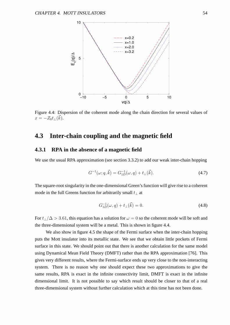
CHAPTER 4. MOTT INSULATORS 54
Figure 4.4: Dispersion of the coherent mode along the chain direction for several values ofx = −Z0t⊥(~k).
4.3 Inter-chain coupling and the magnetic field
4.3.1 RPA in the absence of a magnetic field
We use the usual RPA approximation (see section 3.3.2) to addour weak inter-chain hopping
G−1(ω; q,~k) = G−11D(ω, q) + t⊥(~k). (4.7)
The square-root singularity in the one-dimensional Green’s function will give rise to a coherent
mode in the full Greens function for arbitrarily smallt⊥ at
G−11D(ω, q) + t⊥(~k) = 0. (4.8)
For t⊥/∆ > 3.61, this equation has a solution forω = 0 so the coherent mode will be soft and
the three-dimensional system will be a metal. This is shown in figure 4.4.
We also show in figure 4.5 the shape of the Fermi surface when the inter-chain hopping
puts the Mott insulator into its metallic state. We see that we obtain little pockets of Fermi
surface in this state. We should point out that there is another calculation for the same model
using Dynamical Mean Field Theory (DMFT) rather than the RPAapproximation [76]. This
gives very different results, where the Fermi-surface endsup very close to the non-interacting
system. There is no reason why one should expect these two approximations to give the
same results, RPA is exact in the infinite connectivity limit, DMFT is exact in the infinite
dimensional limit. It is not possible to say which result should be closer to that of a real
three-dimensional system without further calculation which at this time has not been done.
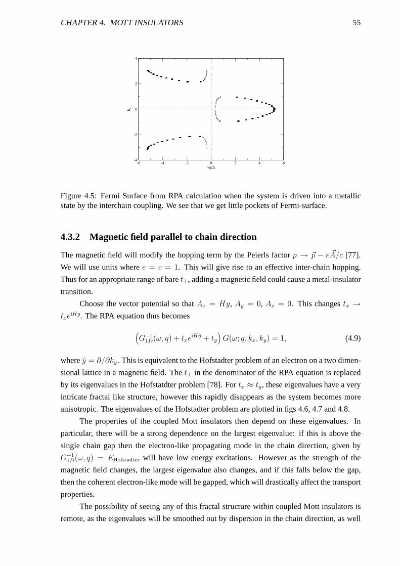
CHAPTER 4. MOTT INSULATORS 55
Figure 4.5: Fermi Surface from RPA calculation when the system is driven into a metallicstate by the interchain coupling. We see that we get little pockets of Fermi-surface.
4.3.2 Magnetic field parallel to chain direction
The magnetic field will modify the hopping term by the Peierlsfactor p → ~p − e ~A/c [77].
We will use units wheree = c = 1. This will give rise to an effective inter-chain hopping.
Thus for an appropriate range of baret⊥, adding a magnetic field could cause a metal-insulator
transition.
Choose the vector potential so thatAx = Hy, Ay = 0, Az = 0. This changestx →txe
iHy. The RPA equation thus becomes
(
G−11D(ω, q) + txe
iHy + ty)
G(ω; q, kx, ky) = 1, (4.9)
wherey = ∂/∂ky. This is equivalent to the Hofstadter problem of an electronon a two dimen-
sional lattice in a magnetic field. Thet⊥ in the denominator of the RPA equation is replaced
by its eigenvalues in the Hofstatdter problem [78]. Fortx ≈ ty, these eigenvalues have a very
intricate fractal like structure, however this rapidly disappears as the system becomes more
anisotropic. The eigenvalues of the Hofstadter problem areplotted in figs 4.6, 4.7 and 4.8.
The properties of the coupled Mott insulators then depend onthese eigenvalues. In
particular, there will be a strong dependence on the largesteigenvalue: if this is above the
single chain gap then the electron-like propagating mode inthe chain direction, given by
G−11D(ω, q) = EHofstadter will have low energy excitations. However as the strength ofthe
magnetic field changes, the largest eigenvalue also changes, and if this falls below the gap,
then the coherent electron-like mode will be gapped, which will drastically affect the transport
properties.
The possibility of seeing any of this fractal structure within coupled Mott insulators is
remote, as the eigenvalues will be smoothed out by dispersion in the chain direction, as well
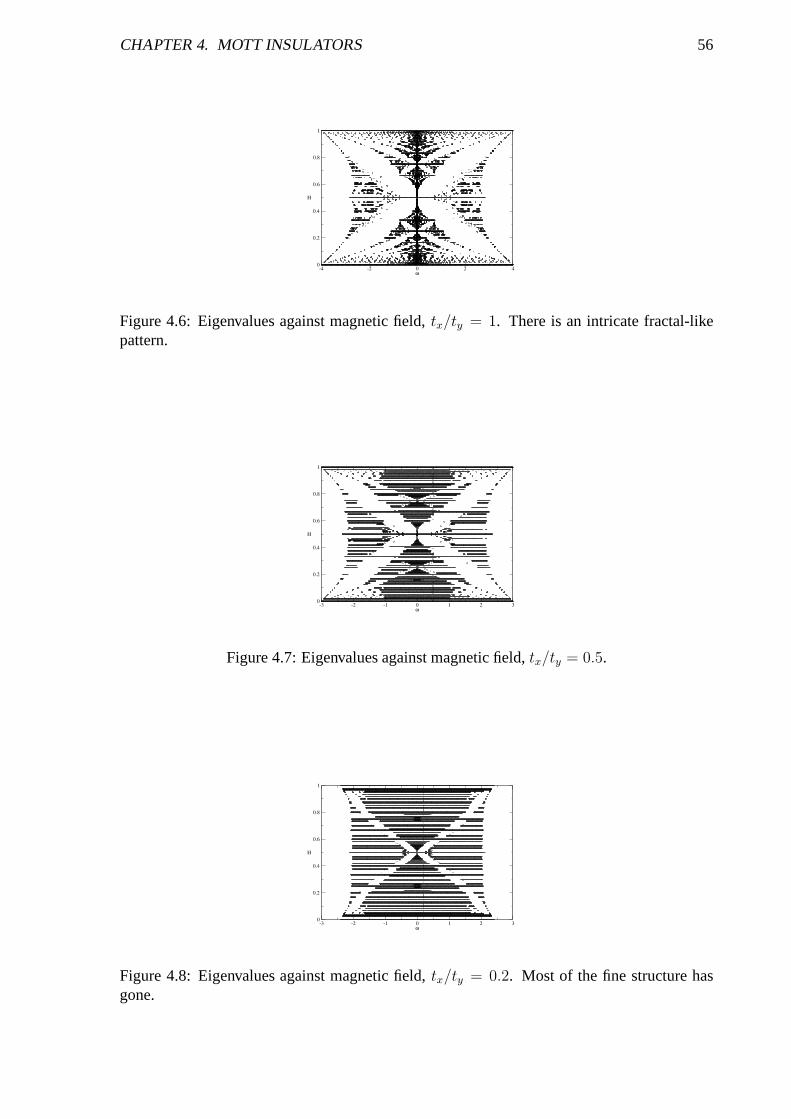
CHAPTER 4. MOTT INSULATORS 56
Figure 4.6: Eigenvalues against magnetic field,tx/ty = 1. There is an intricate fractal-likepattern.
Figure 4.7: Eigenvalues against magnetic field,tx/ty = 0.5.
Figure 4.8: Eigenvalues against magnetic field,tx/ty = 0.2. Most of the fine structure hasgone.
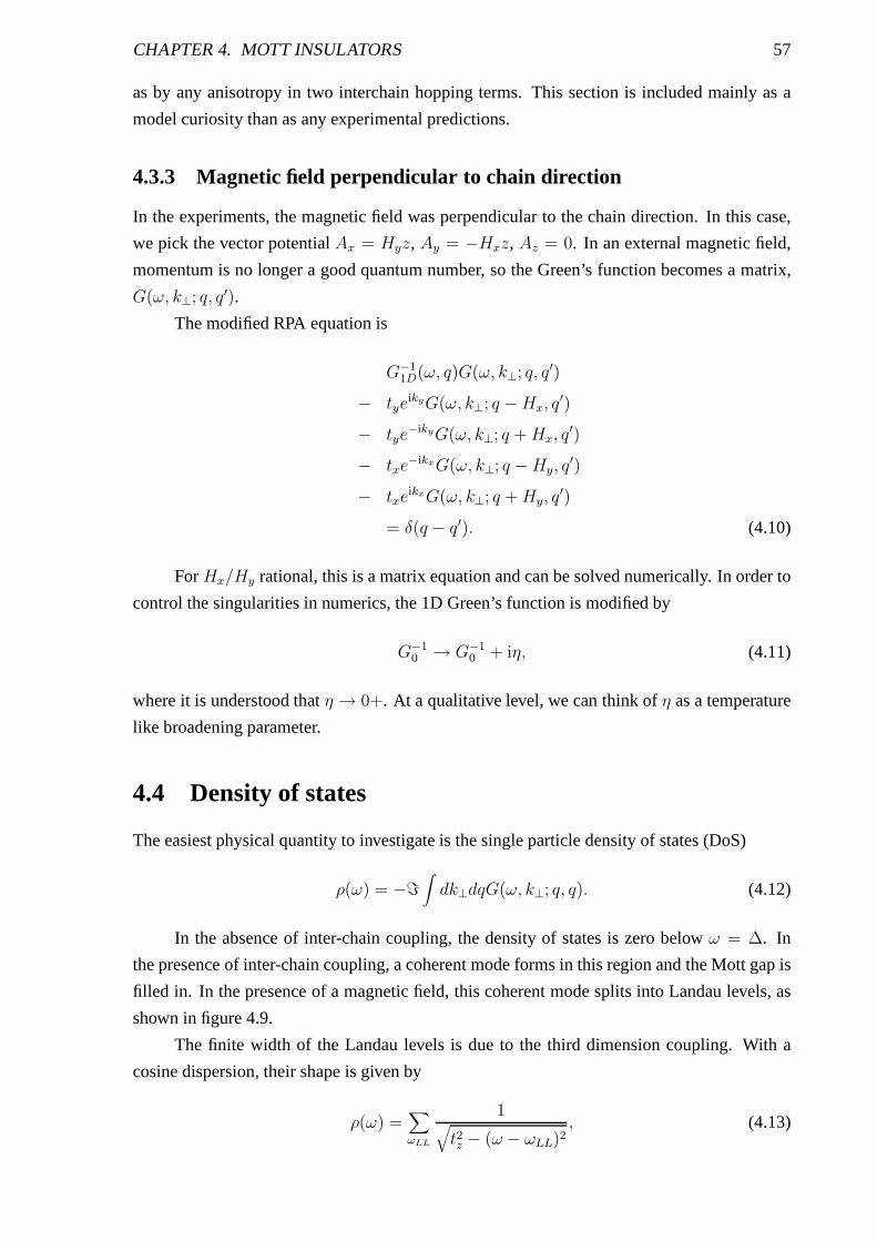
CHAPTER 4. MOTT INSULATORS 57
as by any anisotropy in two interchain hopping terms. This section is included mainly as a
model curiosity than as any experimental predictions.
4.3.3 Magnetic field perpendicular to chain direction
In the experiments, the magnetic field was perpendicular to the chain direction. In this case,
we pick the vector potentialAx = Hyz, Ay = −Hxz, Az = 0. In an external magnetic field,
momentum is no longer a good quantum number, so the Green’s function becomes a matrix,
G(ω, k⊥; q, q′).
The modified RPA equation is
G−11D(ω, q)G(ω, k⊥; q, q′)
− tyeikyG(ω, k⊥; q −Hx, q
′)
− tye−ikyG(ω, k⊥; q +Hx, q
′)
− txe−ikxG(ω, k⊥; q −Hy, q
′)
− txeikxG(ω, k⊥; q +Hy, q
′)
= δ(q − q′). (4.10)
ForHx/Hy rational, this is a matrix equation and can be solved numerically. In order to
control the singularities in numerics, the 1D Green’s function is modified by
G−10 → G−1
0 + iη, (4.11)
where it is understood thatη → 0+. At a qualitative level, we can think ofη as a temperature
like broadening parameter.
4.4 Density of states
The easiest physical quantity to investigate is the single particle density of states (DoS)
ρ(ω) = −ℑ∫
dk⊥dqG(ω, k⊥; q, q). (4.12)
In the absence of inter-chain coupling, the density of states is zero belowω = ∆. In
the presence of inter-chain coupling, a coherent mode formsin this region and the Mott gap is
filled in. In the presence of a magnetic field, this coherent mode splits into Landau levels, as
shown in figure 4.9.
The finite width of the Landau levels is due to the third dimension coupling. With a
cosine dispersion, their shape is given by
ρ(ω) =∑
ωLL
1√
t2z − (ω − ωLL)2, (4.13)
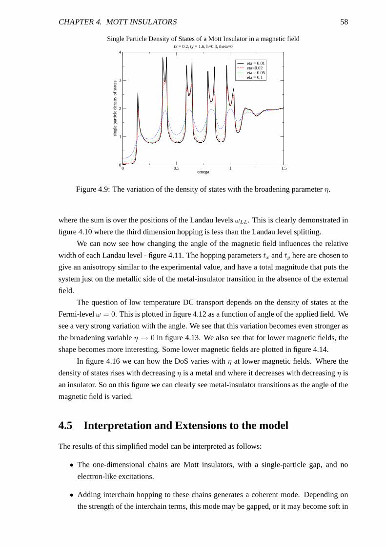
CHAPTER 4. MOTT INSULATORS 58
0 0.5 1 1.5omega
0
1
2
3
4
sing
le p
artic
le d
ensi
ty o
f sta
tes
eta = 0.01eta=0.02eta = 0.05eta = 0.1
Single Particle Density of States of a Mott Insulator in a magnetic fieldtx = 0.2, ty = 1.6, h=0.3, theta=0
Figure 4.9: The variation of the density of states with the broadening parameterη.
where the sum is over the positions of the Landau levelsωLL. This is clearly demonstrated in
figure 4.10 where the third dimension hopping is less than theLandau level splitting.
We can now see how changing the angle of the magnetic field influences the relative
width of each Landau level - figure 4.11. The hopping parameters tx andty here are chosen to
give an anisotropy similar to the experimental value, and have a total magnitude that puts the
system just on the metallic side of the metal-insulator transition in the absence of the external
field.
The question of low temperature DC transport depends on the density of states at the
Fermi-levelω = 0. This is plotted in figure 4.12 as a function of angle of the applied field. We
see a very strong variation with the angle. We see that this variation becomes even stronger as
the broadening variableη → 0 in figure 4.13. We also see that for lower magnetic fields, the
shape becomes more interesting. Some lower magnetic fields are plotted in figure 4.14.
In figure 4.16 we can how the DoS varies withη at lower magnetic fields. Where the
density of states rises with decreasingη is a metal and where it decreases with decreasingη is
an insulator. So on this figure we can clearly see metal-insulator transitions as the angle of the
magnetic field is varied.
4.5 Interpretation and Extensions to the model
The results of this simplified model can be interpreted as follows:
• The one-dimensional chains are Mott insulators, with a single-particle gap, and no
electron-like excitations.
• Adding interchain hopping to these chains generates a coherent mode. Depending on
the strength of the interchain terms, this mode may be gapped, or it may become soft in
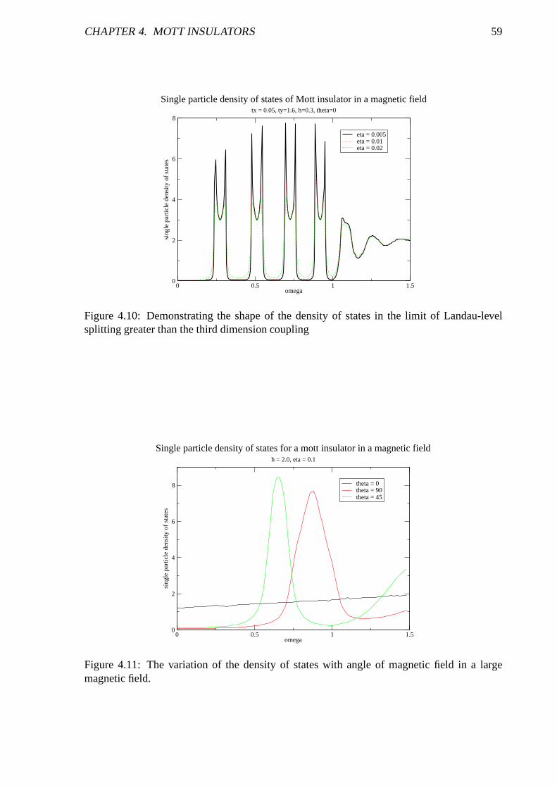
CHAPTER 4. MOTT INSULATORS 59
0 0.5 1 1.5omega
0
2
4
6
8
sing
le p
artic
le d
ensi
ty o
f sta
tes
eta = 0.005eta = 0.01eta = 0.02
Single particle density of states of Mott insulator in a magnetic fieldtx = 0.05, ty=1.6, h=0.3, theta=0
Figure 4.10: Demonstrating the shape of the density of states in the limit of Landau-levelsplitting greater than the third dimension coupling
0 0.5 1 1.5omega
0
2
4
6
8
sing
le p
artic
le d
ensi
ty o
f sta
tes
theta = 0theta = 90theta = 45
Single particle density of states for a mott insulator in a magnetic fieldh = 2.0, eta = 0.1
Figure 4.11: The variation of the density of states with angle of magnetic field in a largemagnetic field.
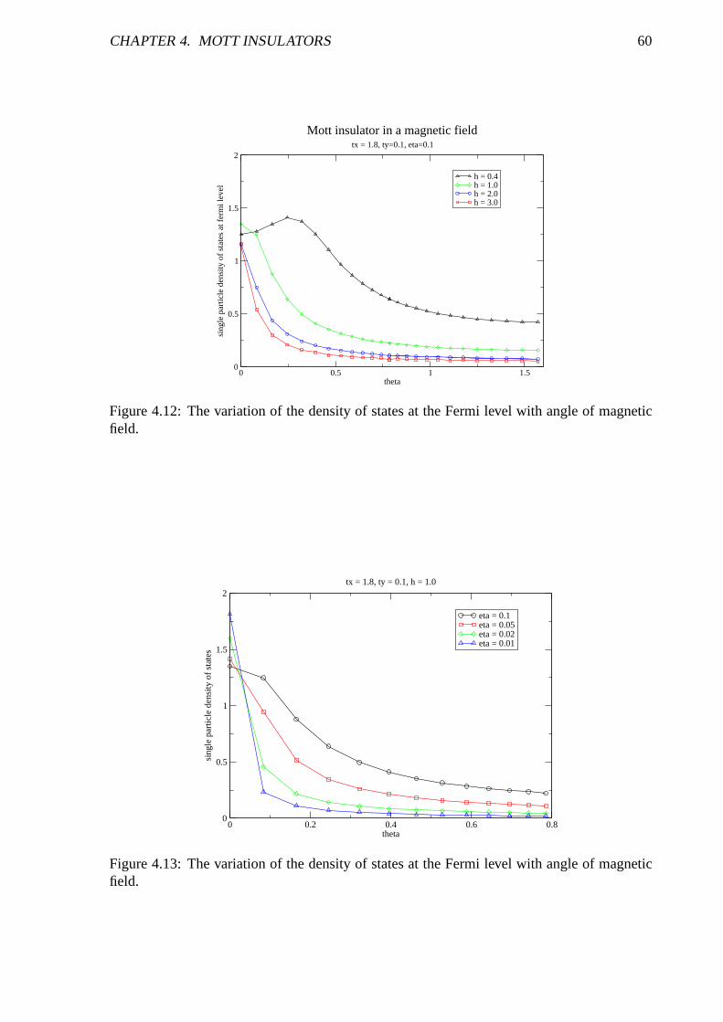
CHAPTER 4. MOTT INSULATORS 60
0 0.5 1 1.5theta
0
0.5
1
1.5
2
sing
le p
artic
le d
ensi
ty o
f sta
tes
at fe
rmi l
evel h = 0.4
h = 1.0h = 2.0h = 3.0
Mott insulator in a magnetic fieldtx = 1.8, ty=0.1, eta=0.1
Figure 4.12: The variation of the density of states at the Fermi level with angle of magneticfield.
0 0.2 0.4 0.6 0.8theta
0
0.5
1
1.5
2
sing
le p
artic
le d
ensi
ty o
f sta
tes
eta = 0.1eta = 0.05eta = 0.02eta = 0.01
tx = 1.8, ty = 0.1, h = 1.0
Figure 4.13: The variation of the density of states at the Fermi level with angle of magneticfield.
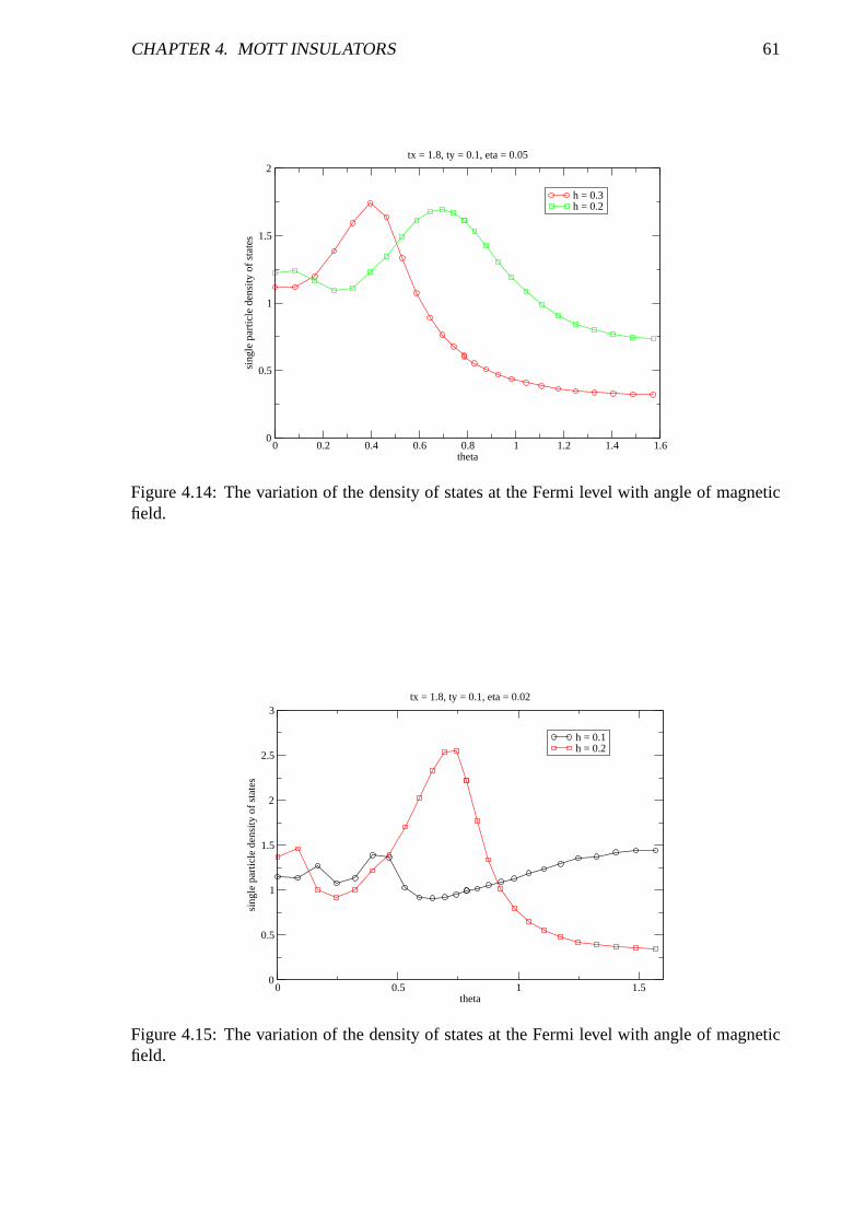
CHAPTER 4. MOTT INSULATORS 61
0 0.2 0.4 0.6 0.8 1 1.2 1.4 1.6theta
0
0.5
1
1.5
2
sing
le p
artic
le d
ensi
ty o
f sta
tes
h = 0.3h = 0.2
tx = 1.8, ty = 0.1, eta = 0.05
Figure 4.14: The variation of the density of states at the Fermi level with angle of magneticfield.
0 0.5 1 1.5theta
0
0.5
1
1.5
2
2.5
3
sing
le p
artic
le d
ensi
ty o
f sta
tes
h = 0.1h = 0.2
tx = 1.8, ty = 0.1, eta = 0.02
Figure 4.15: The variation of the density of states at the Fermi level with angle of magneticfield.
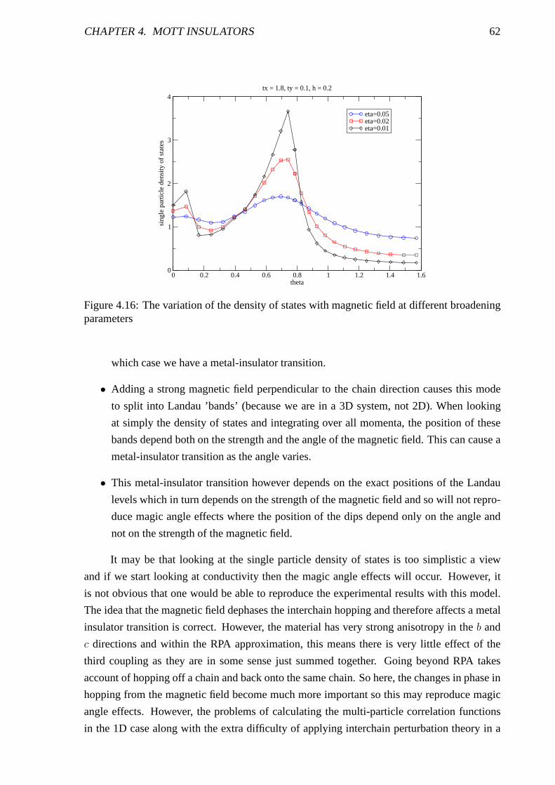
CHAPTER 4. MOTT INSULATORS 62
0 0.2 0.4 0.6 0.8 1 1.2 1.4 1.6theta
0
1
2
3
4
sing
le p
artic
le d
ensi
ty o
f sta
tes
eta=0.05eta=0.02eta=0.01
tx = 1.8, ty = 0.1, h = 0.2
Figure 4.16: The variation of the density of states with magnetic field at different broadeningparameters
which case we have a metal-insulator transition.
• Adding a strong magnetic field perpendicular to the chain direction causes this mode
to split into Landau ’bands’ (because we are in a 3D system, not 2D). When looking
at simply the density of states and integrating over all momenta, the position of these
bands depend both on the strength and the angle of the magnetic field. This can cause a
metal-insulator transition as the angle varies.
• This metal-insulator transition however depends on the exact positions of the Landau
levels which in turn depends on the strength of the magnetic field and so will not repro-
duce magic angle effects where the position of the dips depend only on the angle and
not on the strength of the magnetic field.
It may be that looking at the single particle density of states is too simplistic a view
and if we start looking at conductivity then the magic angle effects will occur. However, it
is not obvious that one would be able to reproduce the experimental results with this model.
The idea that the magnetic field dephases the interchain hopping and therefore affects a metal
insulator transition is correct. However, the material hasvery strong anisotropy in theb and
c directions and within the RPA approximation, this means there is very little effect of the
third coupling as they are in some sense just summed together. Going beyond RPA takes
account of hopping off a chain and back onto the same chain. Sohere, the changes in phase in
hopping from the magnetic field become much more important sothis may reproduce magic
angle effects. However, the problems of calculating the multi-particle correlation functions
in the 1D case along with the extra difficulty of applying interchain perturbation theory in a
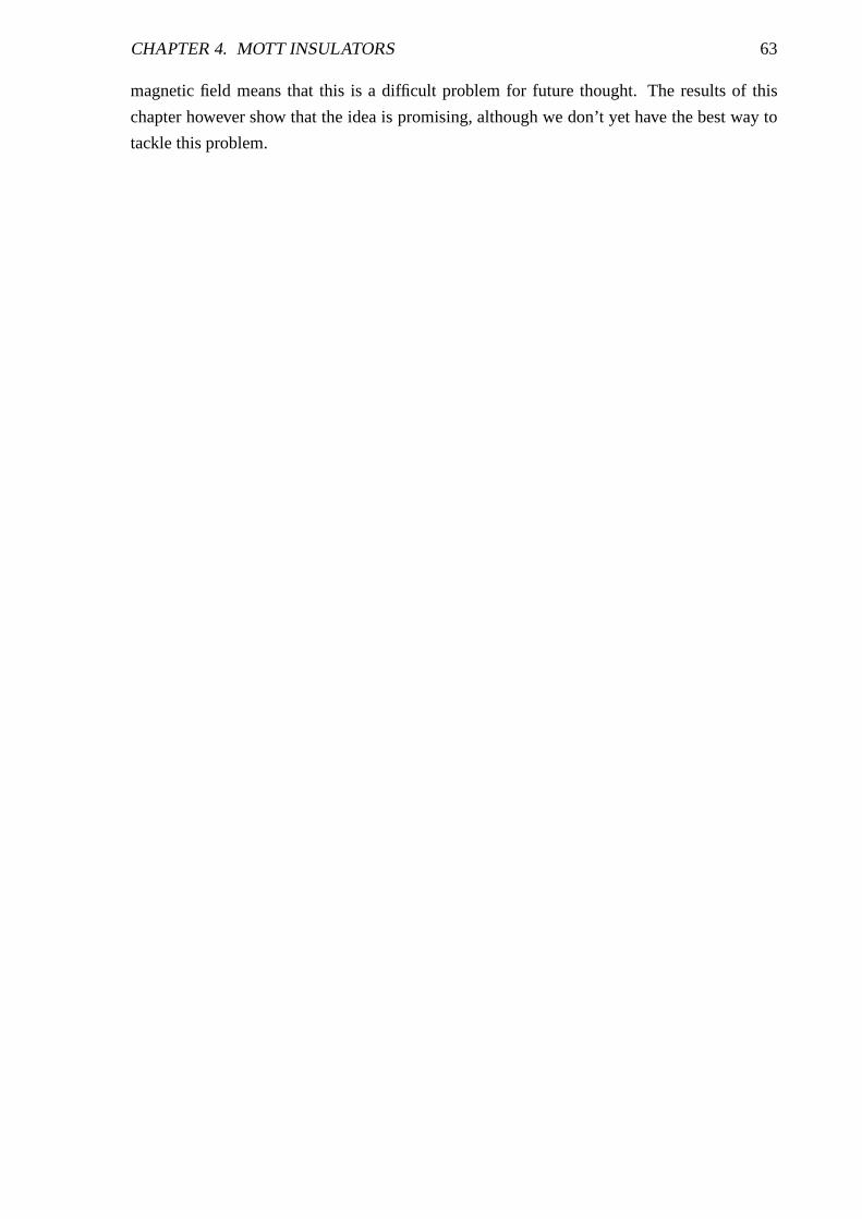
CHAPTER 4. MOTT INSULATORS 63
magnetic field means that this is a difficult problem for future thought. The results of this
chapter however show that the idea is promising, although wedon’t yet have the best way to
tackle this problem.
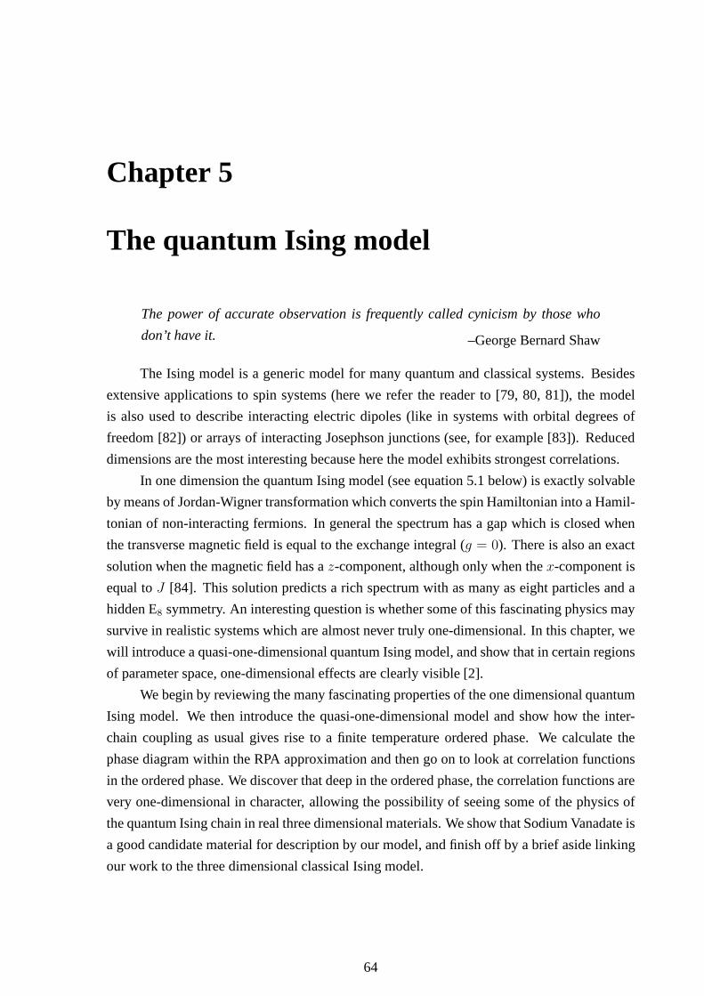
Chapter 5
The quantum Ising model
The power of accurate observation is frequently called cynicism by those who
don’t have it. –George Bernard Shaw
The Ising model is a generic model for many quantum and classical systems. Besides
extensive applications to spin systems (here we refer the reader to [79, 80, 81]), the model
is also used to describe interacting electric dipoles (likein systems with orbital degrees of
freedom [82]) or arrays of interacting Josephson junctions(see, for example [83]). Reduced
dimensions are the most interesting because here the model exhibits strongest correlations.
In one dimension the quantum Ising model (see equation 5.1 below) is exactly solvable
by means of Jordan-Wigner transformation which converts the spin Hamiltonian into a Hamil-
tonian of non-interacting fermions. In general the spectrum has a gap which is closed when
the transverse magnetic field is equal to the exchange integral (g = 0). There is also an exact
solution when the magnetic field has az-component, although only when thex-component is
equal toJ [84]. This solution predicts a rich spectrum with as many as eight particles and a
hidden E8 symmetry. An interesting question is whether some of this fascinating physics may
survive in realistic systems which are almost never truly one-dimensional. In this chapter, we
will introduce a quasi-one-dimensional quantum Ising model, and show that in certain regions
of parameter space, one-dimensional effects are clearly visible [2].
We begin by reviewing the many fascinating properties of theone dimensional quantum
Ising model. We then introduce the quasi-one-dimensional model and show how the inter-
chain coupling as usual gives rise to a finite temperature ordered phase. We calculate the
phase diagram within the RPA approximation and then go on to look at correlation functions
in the ordered phase. We discover that deep in the ordered phase, the correlation functions are
very one-dimensional in character, allowing the possibility of seeing some of the physics of
the quantum Ising chain in real three dimensional materials. We show that Sodium Vanadate is
a good candidate material for description by our model, and finish off by a brief aside linking
our work to the three dimensional classical Ising model.
64
CHAPTER 5. THE QUANTUM ISING MODEL 65
5.1 The one dimensional quantum Ising model
5.1.1 The model atT = 0
A full review of all the work done on the one-dimensional quantum Ising model is the subject
of an entire book by itself, see for example [79, 80, 81]. Herewe give a concise, self contained
but by no means complete review of the model, concentrating in particular on the results that
will be useful later.
The quantum Ising model was first introduced by De Gennes [85]to model the order-
disorder transition in double-well ferroelectric materials, for example KH2PO4. Each proton
of the hydrogen bond can occupy one of two minima of a double well created by the oxygen
atoms. These two possibilities are are represented by a pseudo-spin at each site, withσz =
+1/2 corresponding to one of the minima andσz = −1/2 the other. The operatorσx is then
a tunnelling term between the two minima; including also electrostatic dipolar interaction
between neighbouring sites gives the effective low-energypseudo-spin Hamiltonian
H1D = −J∑
n
{
σznσzn+1 + (1 + g)σxn
}
. (5.1)
The model shows competition between the ordering termJ and the tunnelling termJ(1 + g).
This model has a hidden symmetry, involving dual fields. Define a dual lattice{n+1/2}with fields defined by
µzn+1/2 =n∏
j=1
σxj ,
σzn =n−1∏
j=1
µxj+1/2, (5.2)
so that
µzn−1/2µzn+1/2 = σxn,
σznσzn+1 = µxn+1/2. (5.3)
In terms of the new variables, the Hamiltonian preserves itsform
H1D = −J(1 + g)∑
n
(
µzn−1/2µzn+1/2 +
1
1 + gµxn+1/2
)
. (5.4)
We see that the self-duality point isg = 0 - as we will show later this corresponds to a quantum
phase transition. Theµ fields are sometimes known as the disorder operators.
The model can be solved by a Jordan-Wigner transformation. We write
σxn = 2a†nan − 1,
CHAPTER 5. THE QUANTUM ISING MODEL 66
g
T
0
quantumcritical
ordered
Low TLow T
Figure 5.1: Phase Diagram of model (5.1). AtT = 0 there is an ordered phase forg < 0which has〈σz〉 6= 0. For T = 0 andg > 0, the system is a quantum paramagnet, and bythe duality 5.2, we have〈µz〉 6= 0 in this region. At finite temperature, long range order isforbidden by the Mermin Wagner theorem. There are crossovers (given by the dashed lines)where the single-particle energy gap∆ ∼ T between the low-temperature behaviour and auniversal quantum critical regime.
σzn = (−1)n−1 exp
iπn−1∑
j=1
a†jaj
(a†n + an), (5.5)
where the Fermi operatorsa satisfy the usual anti-commutation relations
{
an, a†m
}
= δnm, {an, am} = 0. (5.6)
The Hamiltonian becomes quadratic
H1D = J∑
n
[
−(a†n − an)((a†n+1 + an+1) + (g + 1)(a†n − an)(a
†n + an)
]
, (5.7)
which can be easily diagonalised to give the spectrum
ǫ(k) = 2J√
g2 + 4(g + 1) sin2(k/2). (5.8)
We see that this is gapless atg = 0 where the model is critical. Forg < 0 the model is an a
’quantum ordered’ phase where〈σz〉 6= 0 at T = 0. For g > 0 it is a ’quantum disordered
phase’ where in fact〈µz〉 6= 0 atT = 0. The phase diagram is shown in figure 5.1.
Although we have mapped the model on to free fermions and thereby solved it exactly,
it is still not easy to extract spin-spin correlation functions because our transformation was
non-local in space. The correlation functions are most easily calculated in terms of a form
factor expansion - see section 2.2.2 and also [86].
The relevant minimal form factors were calculated in section 2.2.2:
F(n)min(θ1, . . . , θn) =
∏
i<j
tanh
(
θi − θj2
)
, (5.9)
CHAPTER 5. THE QUANTUM ISING MODEL 67
wheren is odd for correlators ofσz and even for correlators ofµz (in the disordered phase).
To lowest order, the correlation function is
χ1D(ω, k) =Z0(ma0/v)
1/4
ω2 − (vk)2 −m2, (5.10)
whereZ0 = 1.8437 is fixed by the conformal normalisation 5.21 of the field operators. This
is valid for smallω. In real space, it corresponds to long distance asymptotics
χ1D(r) =Z0(ma0/v)
1/4
πK0(mr) +O(e−3r) (5.11)
The next term in the form factor expansion, the three particle contribution can be repre-
sented as
χ3(s2)
χ1(s = 0)=
1
3
∫ dx
4π
∫ dy
4π
f(2x)f(y + x)f(y − x)
(s/m)2 − [1 + 4 coshx(cosh x+ cosh y)],
f(x) = tanh2(x/2), (5.12)
wheres2 = ω2− (vk)2 and is plotted in Fig. 5.2. The imaginary part of this term (which is the
contribution to the structure factor) and of all higher terms in the series is zero belowω = 3m,
however all terms in the expansion contribute towards the real part atω = 0. Fortunately
the contribution from higher order terms1 are negligible at smalls (see e.g. [88]). We see
explicitly in this case thatχ3(s = 0)/χ1(s = 0) = 0.0002 so that 5.10 is indeed a very good
approximation for smalls.
5.1.2 The model at finite temperature - scaling behaviour
The correlation functions at finite but low temperature can be well approximated[79] by adding
the quantum dephasing time,τψ, into equation 5.10:
χ1D(ω, k) =Z0(ma0/v)
1/4
(ω + i/τψ)2 − (vk)2 −m2. (5.15)
1In fact, for this model it turns out one can sum all the terms inthe series and write the result exactly in termsof the solution of a Painleve equation [86]:
〈σ(r)σ(0)〉 = sinhχ(s)
2exp
{
−1
4
∫
∞
s
duu
[
(
dχ
du
)2
− sinh2 χ
]}
(5.13)
wheres is the scaling variables = mr/2 andχ(s) is a solution of the radial sinh-Gordon equation
d2χ
ds2+
1
s
dχ
ds= 2 sinh(2χ) (5.14)
which under the transformationη = e−χ is equivalent to the Painleve III equation [87]. The abilityto writecorrelation functions in terms of non-linear differentialequations seems to be specific to this model, and althougha very nice result, is not that useful in terms of extracting low energy behaviour.
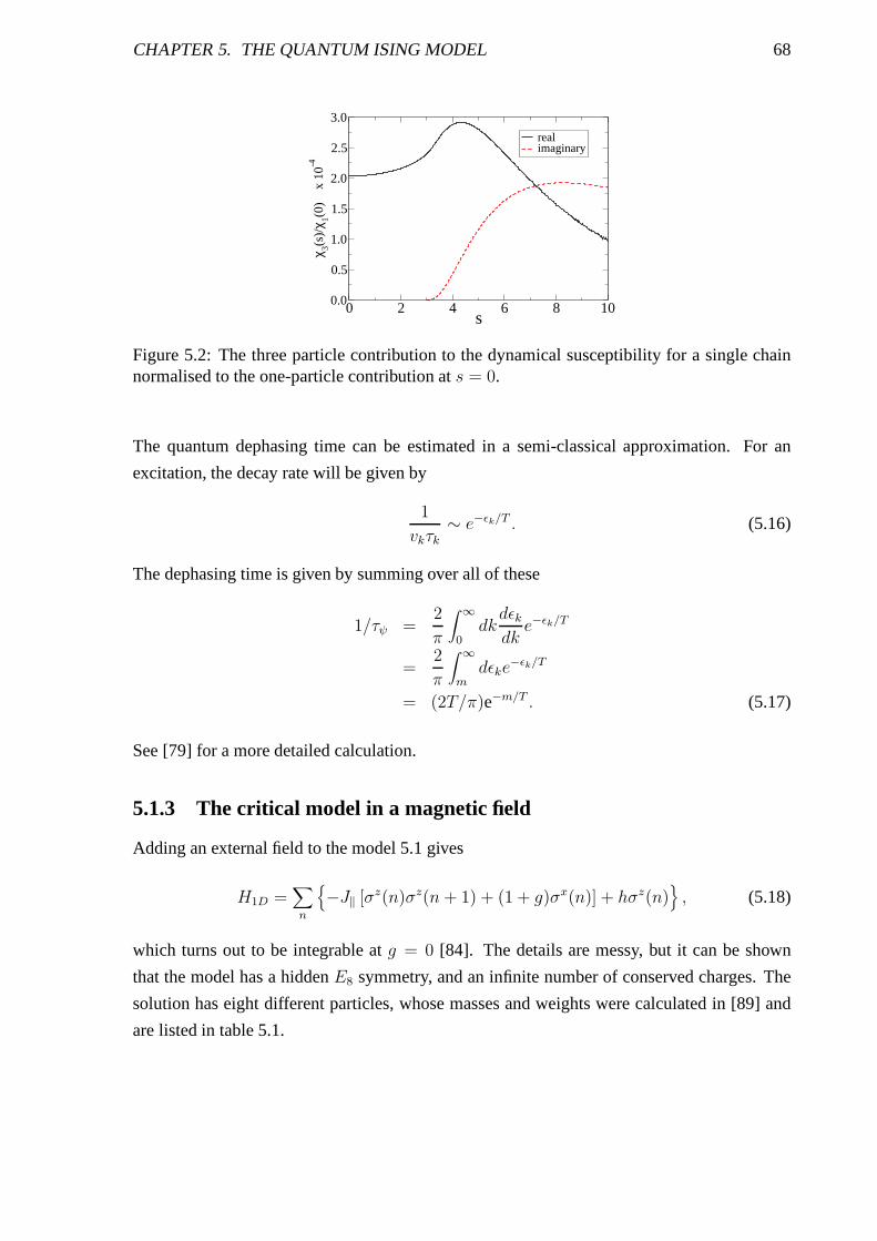
CHAPTER 5. THE QUANTUM ISING MODEL 68
0 2 4 6 8 10s
0.0
0.5
1.0
1.5
2.0
2.5
3.0
χ 3(s)/χ
1(0)
x
10-4
realimaginary
Figure 5.2: The three particle contribution to the dynamical susceptibility for a single chainnormalised to the one-particle contribution ats = 0.
The quantum dephasing time can be estimated in a semi-classical approximation. For an
excitation, the decay rate will be given by
1
vkτk∼ e−ǫk/T . (5.16)
The dephasing time is given by summing over all of these
1/τψ =2
π
∫ ∞
0dkdǫkdk
e−ǫk/T
=2
π
∫ ∞
mdǫke
−ǫk/T
= (2T/π)e−m/T . (5.17)
See [79] for a more detailed calculation.
5.1.3 The critical model in a magnetic field
Adding an external field to the model 5.1 gives
H1D =∑
n
{
−J‖ [σz(n)σz(n + 1) + (1 + g)σx(n)] + hσz(n)}
, (5.18)
which turns out to be integrable atg = 0 [84]. The details are messy, but it can be shown
that the model has a hiddenE8 symmetry, and an infinite number of conserved charges. The
solution has eight different particles, whose masses and weights were calculated in [89] and
are listed in table 5.1.
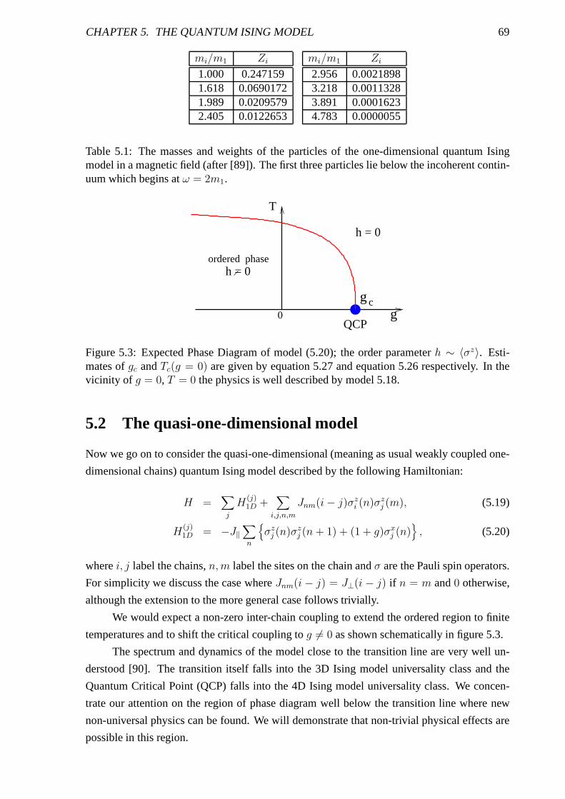
CHAPTER 5. THE QUANTUM ISING MODEL 69
mi/m1 Zi
1.000 0.2471591.618 0.06901721.989 0.02095792.405 0.0122653
mi/m1 Zi
2.956 0.00218983.218 0.00113283.891 0.00016234.783 0.0000055
Table 5.1: The masses and weights of the particles of the one-dimensional quantum Isingmodel in a magnetic field (after [89]). The first three particles lie below the incoherent contin-uum which begins atω = 2m1.
gc
h = 0
g
T
0
h = 0
QCP
ordered phase
Figure 5.3: Expected Phase Diagram of model (5.20); the order parameterh ∼ 〈σz〉. Esti-mates ofgc andTc(g = 0) are given by equation 5.27 and equation 5.26 respectively. In thevicinity of g = 0, T = 0 the physics is well described by model 5.18.
5.2 The quasi-one-dimensional model
Now we go on to consider the quasi-one-dimensional (meaningas usual weakly coupled one-
dimensional chains) quantum Ising model described by the following Hamiltonian:
H =∑
j
H(j)1D +
∑
i,j,n,m
Jnm(i− j)σzi (n)σzj (m), (5.19)
H(j)1D = −J‖
∑
n
{
σzj (n)σzj (n + 1) + (1 + g)σxj (n)}
, (5.20)
wherei, j label the chains,n,m label the sites on the chain andσ are the Pauli spin operators.
For simplicity we discuss the case whereJnm(i − j) = J⊥(i − j) if n = m and0 otherwise,
although the extension to the more general case follows trivially.
We would expect a non-zero inter-chain coupling to extend the ordered region to finite
temperatures and to shift the critical coupling tog 6= 0 as shown schematically in figure 5.3.
The spectrum and dynamics of the model close to the transition line are very well un-
derstood [90]. The transition itself falls into the 3D Isingmodel universality class and the
Quantum Critical Point (QCP) falls into the 4D Ising model universality class. We concen-
trate our attention on the region of phase diagram well belowthe transition line where new
non-universal physics can be found. We will demonstrate that non-trivial physical effects are
possible in this region.
CHAPTER 5. THE QUANTUM ISING MODEL 70
Although model 5.20 is a lattice model, we will be working in the field theoretic limit
where we fix the normalisation of the magnetisation operatorby the standard conformal field
theory condition:
χ1D(τ, x) = 〈σ(τ, x)σ(0)〉 =(a0/v)
1/4
|r|1/4 , |r| → 0, (5.21)
wherer2 = τ 2 + (x/v)2, τ is the Matsubara time,v = J‖a0 is the on-chain velocity anda0 is
the lattice spacing in the chain direction.
There are three energy scales in this problem: the on chain couplingJ‖, the spectral gap
for a single chainm = |g|J‖, and the inter-chain couplingJ⊥. In order to treat the model as
weakly coupled chains we must haveJ⊥ ≪ J‖ and in order to apply the continuous limit field
theoretic techniques to solve the uncoupled chains, we musthavem ≪ J‖. However,m and
J⊥ can both be of the same order of magnitude.
5.2.1 The Phase Diagram
To estimate the critical temperature, we use the RPA to calculate the three dimensional sus-
ceptibility
χ(ω, k;k⊥) = [χ−11D(ω, k) − J⊥(k⊥)]−1, (5.22)
and then look forω = 0 divergences in the correlation function which signify a developing
instability. In this expression,χ1D is the susceptibility of a single chain:
χ1D(ω, k) = −i∑
n
∫ ∞
0dteiωt−ikn〈[σz(t, n), σz(0, 0)]〉. (5.23)
We begin by considering the lineg = 0 where the uncoupled chains are critical. We
showed in section 2.3 that at finite temperature the spin-spin correlation function 5.21 becomes
χ1D(τ, x) =
[
(πTa0/v)2
sinh(πT (x/v − iτ)) sinh(πT (x/v + iτ))
]1/8
. (5.24)
The Fourier transform (5.23) gives the dynamic susceptibility [91]
χ1D(ω = 0, k = 0) =a0
v(2πTa0/v)
−7/4 sinπ
8B2(1/16, 7/8), (5.25)
whereB(x, y) = Γ(x)Γ(y)/Γ(x+y) is the Beta function2. From equation 5.22 we extract the
transition temperature:
Tc/J‖ = 2.12
[
z⊥J⊥J‖
]4/7
. (5.26)
Now let us estimate the position of the Quantum Critical Point (QCP) on theg axis.
2Note that although the equation contains the rather ill-defined lattice spacing,a0, it is always in the combi-nationv/a0 = J meaning that this equation relates the static susceptibility to the bare parameters independentof any high energy cut-off as it must for a well defined theory.
CHAPTER 5. THE QUANTUM ISING MODEL 71
Again we use the RPA equation (5.22) substituting in the expression for the dynamical spin
susceptibility 5.10 of the off-critical Ising model. We cansee that the QCP whereTc → 0 is
given by the condition
gc ≈ 1.42(z⊥J⊥/J‖)4/7. (5.27)
The RPA expression for the susceptibility at the QCP is
χ(ω, k;k⊥) ∼ 1
ω2 − (vk)2 − (v⊥k⊥)2, (5.28)
wherev⊥ = (1/2)Z0g1/4J‖
(
d2J⊥(k⊥ = 0)/dk2⊥)
. In the vicinity of QCP the low-energy
behaviour of the quantum Ising model is universal and falls in the universality class of the
(d+2)-dimensional classical Ising model, where d is the number of transverse dimensions.
Sinced = 2 corresponds to the upper critical dimension of that model, the fluctuations give
only logarithmic corrections to RPA in three dimensions.
Near the critical point, we can examine the shape of the phaseboundary. For low tem-
perature, the correlation functions at finite temperature can be well approximated by 5.15. The
RPA then gives the condition for a singularity atω = 0, k = 0 as
m2 + 1/τ 2ψ = Z0J‖J⊥g
1/4, (5.29)
so the transition temperature in the vicinity of the critical point is approximately
Tc =m
ln(1/y)− ln ln(1/y),
y =π
2
(
Z0(J⊥/J‖)g−7/4 − 1
)1/2. (5.30)
For g < 0, uncoupled chains are completely ordered atT = 0, and atT > 0 andm not
too small there is order on a length scale
ξc = v(2mT/π)−1/2em/T . (5.31)
A crude estimate for the transition temperature can be is given by
J⊥Tc
(
ξc(Tc)
v/m
)2
∼ 1, (5.32)
which gives
Tc ≈2m
ln(m/J⊥). (5.33)
5.2.2 Dispersion in the ordered phase
In the ordered state expression 5.23 has to be modified. Namely, one has to replaceχ1D by the
dynamical susceptibility calculated in the presence of an effective magnetic field generated by
the neighbouring chains [92]. In other words, in calculating χ1D one has to use the following
CHAPTER 5. THE QUANTUM ISING MODEL 72
Hamiltonian:
H1D =∑
n
{
−J‖ [σz(n)σz(n + 1) + (1 + g)σx(n)] + hσz(n)}
, (5.34)
with the self-consistency relation
h = J⊥(q = 0)〈σz〉. (5.35)
Now we go on to calculate the dispersion and spectrum within the ordered phase, where
we have to considerh 6= 0. Model 5.34 is exactly solvable only atg = 0 [84]. As we
have mentioned, the spectrum consists of eight particles which are listed in table 5.1. The
contributions to the dynamical susceptibility for smallω decline quickly with the growth of
the particle mass and the decrease in spectral weight of the mode. Therefore the magnetic
susceptibility atT = 0 can be well approximated by keeping only the first three polesbelow
the incoherent continuum
χ1D(s) =
(
4m21
15πJ‖h
)2 3∑
i=1
Zis2 −m2
i
, (5.36)
with s defined as before. In this model, the mass scale is given by[93]
m1(h)/J‖ = α1(h/J‖)8/15,
α1 = 4.40490858, (5.37)
and the single-particle expectation value is
〈σz(0)〉 = α2(h/J‖)1/15,
α2 = 1.07496. (5.38)
The self-consistency relations 5.35 therefore give
h/J‖ =[
α2J⊥(0)/J|]15/14
,
m/J‖ = α1
[
α2J⊥(0)/J‖]4/7
. (5.39)
In the RPA 5.22, the dispersion is given by the condition
1
J⊥=
∑
i
Zis2 −m2
i
,
J⊥ =
(
4m21
15πh
)2
J⊥ = α3m21
J⊥(k⊥)
J⊥(0), (5.40)
where the final relation is obtained from the self-consistent relations withα3 = (4/15π)2α21/α2 =
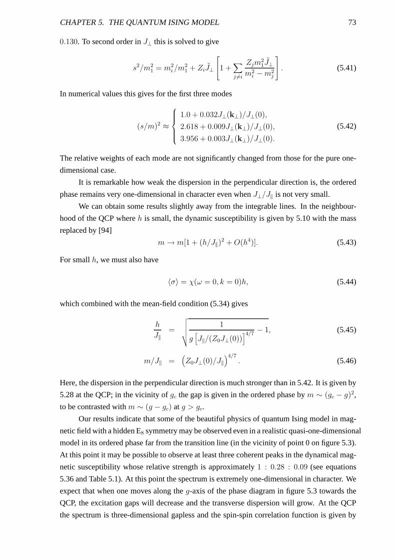
CHAPTER 5. THE QUANTUM ISING MODEL 73
0.130. To second order inJ⊥ this is solved to give
s2/m21 = m2
i /m21 + ZiJ⊥
1 +∑
j 6=i
Zjm21J⊥
m2i −m2
j
. (5.41)
In numerical values this gives for the first three modes
(s/m)2 ≈
1.0 + 0.032J⊥(k⊥)/J⊥(0),
2.618 + 0.009J⊥(k⊥)/J⊥(0),
3.956 + 0.003J⊥(k⊥)/J⊥(0).
(5.42)
The relative weights of each mode are not significantly changed from those for the pure one-
dimensional case.
It is remarkable how weak the dispersion in the perpendicular direction is, the ordered
phase remains very one-dimensional in character even whenJ⊥/J‖ is not very small.
We can obtain some results slightly away from the integrablelines. In the neighbour-
hood of the QCP whereh is small, the dynamic susceptibility is given by 5.10 with the mass
replaced by [94]
m→ m[1 + (h/J‖)2 +O(h4)]. (5.43)
For smallh, we must also have
〈σ〉 = χ(ω = 0, k = 0)h, (5.44)
which combined with the mean-field condition (5.34) gives
h
J‖=
√
√
√
√
√
1
g[
J‖/(Z0J⊥(0))]4/7
− 1, (5.45)
m/J‖ =(
Z0J⊥(0)/J‖)4/7
. (5.46)
Here, the dispersion in the perpendicular direction is muchstronger than in 5.42. It is given by
5.28 at the QCP; in the vicinity ofgc the gap is given in the ordered phase bym ∼ (gc − g)2,
to be contrasted withm ∼ (g − gc) at g > gc.
Our results indicate that some of the beautiful physics of quantum Ising model in mag-
netic field with a hidden E8 symmetry may be observed even in a realistic quasi-one-dimensional
model in its ordered phase far from the transition line (in the vicinity of point 0 on figure 5.3).
At this point it may be possible to observe at least three coherent peaks in the dynamical mag-
netic susceptibility whose relative strength is approximately 1 : 0.28 : 0.09 (see equations
5.36 and Table 5.1). At this point the spectrum is extremely one-dimensional in character. We
expect that when one moves along theg-axis of the phase diagram in figure 5.3 towards the
QCP, the excitation gaps will decrease and the transverse dispersion will grow. At the QCP
the spectrum is three-dimensional gapless and the spin-spin correlation function is given by
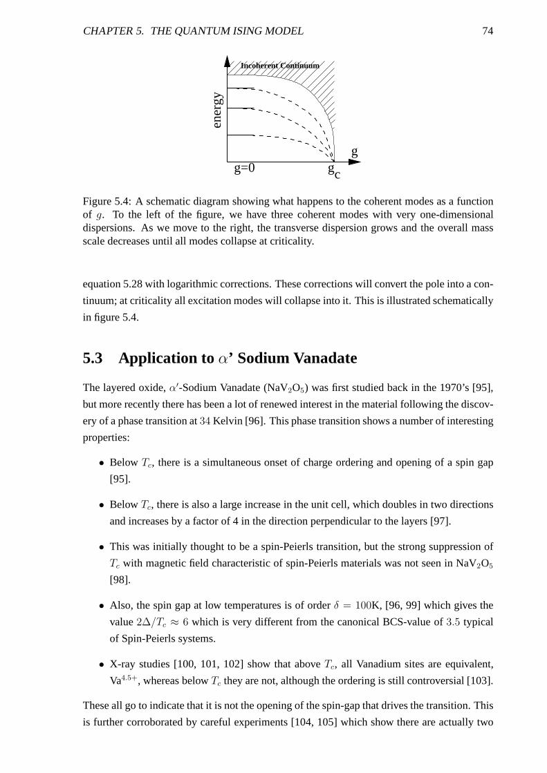
CHAPTER 5. THE QUANTUM ISING MODEL 74
gc
Incoherent Continuum
ener
gy
g=0g
Figure 5.4: A schematic diagram showing what happens to the coherent modes as a functionof g. To the left of the figure, we have three coherent modes with very one-dimensionaldispersions. As we move to the right, the transverse dispersion grows and the overall massscale decreases until all modes collapse at criticality.
equation 5.28 with logarithmic corrections. These corrections will convert the pole into a con-
tinuum; at criticality all excitation modes will collapse into it. This is illustrated schematically
in figure 5.4.
5.3 Application to α’ Sodium Vanadate
The layered oxide,α′-Sodium Vanadate (NaV2O5) was first studied back in the 1970’s [95],
but more recently there has been a lot of renewed interest in the material following the discov-
ery of a phase transition at34 Kelvin [96]. This phase transition shows a number of interesting
properties:
• Below Tc, there is a simultaneous onset of charge ordering and opening of a spin gap
[95].
• BelowTc, there is also a large increase in the unit cell, which doubles in two directions
and increases by a factor of 4 in the direction perpendicularto the layers [97].
• This was initially thought to be a spin-Peierls transition,but the strong suppression of
Tc with magnetic field characteristic of spin-Peierls materials was not seen in NaV2O5
[98].
• Also, the spin gap at low temperatures is of orderδ = 100K, [96, 99] which gives the
value2∆/Tc ≈ 6 which is very different from the canonical BCS-value of3.5 typical
of Spin-Peierls systems.
• X-ray studies [100, 101, 102] show that aboveTc, all Vanadium sites are equivalent,
Va4.5+, whereas belowTc they are not, although the ordering is still controversial [103].
These all go to indicate that it is not the opening of the spin-gap that drives the transition. This
is further corroborated by careful experiments [104, 105] which show there are actually two
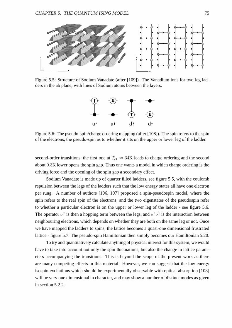
CHAPTER 5. THE QUANTUM ISING MODEL 75
Figure 5.5: Structure of Sodium Vanadate (after [109]). TheVanadium ions for two-leg lad-ders in the ab plane, with lines of Sodium atoms between the layers.
Figure 5.6: The pseudo-spin/charge ordering mapping (after [108]). The spin refers to the spinof the electrons, the pseudo-spin as to whether it sits on theupper or lower leg of the ladder.
second-order transitions, the first one atTc1 ≈ 34K leads to charge ordering and the second
about0.3K lower opens the spin gap. Thus one wants a model in which charge ordering is the
driving force and the opening of the spin gap a secondary effect.
Sodium Vanadate is made up of quarter filled ladders, see figure 5.5, with the coulomb
repulsion between the legs of the ladders such that the low energy states all have one electron
per rung. A number of authors [106, 107] proposed a spin-pseudospin model, where the
spin refers to the real spin of the electrons, and the two eigenstates of the pseudospin refer
to whether a particular electron is on the upper or lower leg of the ladder - see figure 5.6.
The operatorσx is then a hopping term between the legs, andσzσz is the interaction between
neighbouring electrons, which depends on whether they are both on the same leg or not. Once
we have mapped the ladders to spins, the lattice becomes a quasi-one dimensional frustrated
lattice - figure 5.7. The pseudo-spin Hamiltonian then simply becomes our Hamiltonian 5.20.
To try and quantitatively calculate anything of physical interest for this system, we would
have to take into account not only the spin fluctuations, but also the change in lattice param-
eters accompanying the transitions. This is beyond the scope of the present work as there
are many competing effects in this material. However, we cansuggest that the low energy
isospin excitations which should be experimentally observable with optical absorption [108]
will be very one dimensional in character, and may show a number of distinct modes as given
in section 5.2.2.
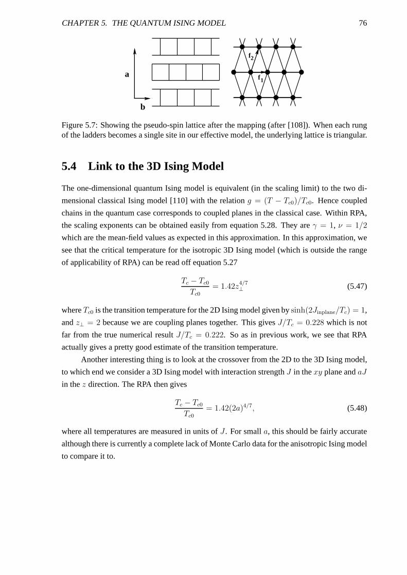
CHAPTER 5. THE QUANTUM ISING MODEL 76
1a
b
f
f2
Figure 5.7: Showing the pseudo-spin lattice after the mapping (after [108]). When each rungof the ladders becomes a single site in our effective model, the underlying lattice is triangular.
5.4 Link to the 3D Ising Model
The one-dimensional quantum Ising model is equivalent (in the scaling limit) to the two di-
mensional classical Ising model [110] with the relationg = (T − Tc0)/Tc0. Hence coupled
chains in the quantum case corresponds to coupled planes in the classical case. Within RPA,
the scaling exponents can be obtained easily from equation 5.28. They areγ = 1, ν = 1/2
which are the mean-field values as expected in this approximation. In this approximation, we
see that the critical temperature for the isotropic 3D Isingmodel (which is outside the range
of applicability of RPA) can be read off equation 5.27
Tc − Tc0Tc0
= 1.42z4/7⊥ (5.47)
whereTc0 is the transition temperature for the 2D Ising model given bysinh(2Jinplane/Tc) = 1,
andz⊥ = 2 because we are coupling planes together. This givesJ/Tc = 0.228 which is not
far from the true numerical resultJ/Tc = 0.222. So as in previous work, we see that RPA
actually gives a pretty good estimate of the transition temperature.
Another interesting thing is to look at the crossover from the 2D to the 3D Ising model,
to which end we consider a 3D Ising model with interaction strengthJ in thexy plane andaJ
in thez direction. The RPA then gives
Tc − Tc0Tc0
= 1.42(2a)4/7, (5.48)
where all temperatures are measured in units ofJ . For smalla, this should be fairly accurate
although there is currently a complete lack of Monte Carlo data for the anisotropic Ising model
to compare it to.
Chapter 6
Final remarks
Like Olympic medals and trophies, all it signifies is that thereceiver has done
something of no use to anybody a little better than everybodyelse.
–Joseph Heller (Catch 22)
In this thesis we were looking at selected models of stronglycorrelated electrons. The
models were all quasi-one-dimensional so we could use a particular recipe to solve them;
namely solving the one dimensional subsystem exactly by means of powerful non-perturbative
techniques and then adding in some higher-dimensional coupling perturbatively.
• We first considered a model of unconventional superconductivity, introduced as a possi-
ble model for High-Tc materials in a stripe phase, but more easily applied to structurally
one-dimensional compounds. Within the RPA approximation we calculated the transi-
tion temperature for generalKc. We calculated the ratioTc/∆c where∆c is the zero
temperature gap in the charge sector. We saw that this decreases below the BCS value
as the coupling strength is increased. We also looked at the properties of our model
in a magnetic field, noting in particular the extreme anisotropy of the phase diagram,
and the possibility of SC-CDW transitions as you vary strength or even angle of mag-
netic field. We then went on to calculate the first correctionsto Tc in the vicinity of
the critical point which is decreased because of the interplay between the two interac-
tions. We finally showed that in two dimensions where RPA breaks down completely,
we get a transition of the Kosterlitz-Thouless type which has the same energy scales as
the ordering transition in higher dimensions.
• We then went on to consider unusual magneto-resistance properties measured in Bech-
gaard salts, namely large dips in the magneto-resistance at’magic angles’, with a corre-
sponding insulator-metal transition in the temperature dependence at these points. Our
model consisted of one-dimensional Mott insulating chainswith enough interchain hop-
ping to drive the system to a metallic state. We concentratedon calculating the density
of states as a function of the strength and angle of the magnetic field. We showed that
although our model had some of the properties needed to explain the measured results,
it was oversimplified and although promising in some respects, did not reproduce the
77
CHAPTER 6. FINAL REMARKS 78
magic angle effects seen in experiments. We suggested several extensions to the model
which may be necessary to explain this phenomena.
• We finished by considered a model of coupled quantum Ising chains. We saw that
within the RPA approximation, we could calculate the phase diagram of the model and
the dispersion in the ordered phase. The most interesting thing is how one dimensional
the excitations are in the three dimensional ordered phase.
Throughout this work, we have tried to motivate much of our theory from real materials.
As real materials are always far more complicated than our simplified models, the application
of the models to the materials has been mostly only at the qualitative level. However we see
the solution of these models as a starting point to make more detailed calculations on individ-
ual materials. Executing these more specific calculations,as well as attempting to refine our
general solutions by going beyond RPA are obvious future directions for research. The overall
message from this thesis is that the world of many electrons still has many unexplored pos-
sibilities. And starting from somewhere different than simply turning the e-e interactions off
can give a lot of insight into the strange and wonderful worldof strongly correlated systems.
Bibliography
[1] S.T.Carr and A.M.Tsvelik, Phys. Rev. B65, 195121 (2002).
[2] S.T.Carr and A.M.Tsvelik, Phys. Rev. Lett.90, 177206 (2003).
[3] L.D.Landau, Soviet Physics JETP3, 920 (1957).
[4] A.A.Abrikosov, L.P.Gorkov, and I.E.Dzyaloshinski,Methods of Quantum Field Theory
in Statistical Physics(Dover, New York, 1963).
[5] D.Senechal, cond-mat/9908262 (1999).
[6] S.Tomonaga, Prog. Theor. Phys. (Kyoto)5, 544 (1950).
[7] J.M.Luttinger, J.Math. Phys.4, 1154 (1963).
[8] D.C.Mattis and E.H.Lieb, J. Math. Phys.6, 304 (1965).
[9] R.Heidenreich, B.Schroer, R.Seiler, and D.Uhlenbrock, Phys. Lett.54, 119 (1975).
[10] A.Luther and I.Peschel, Phys. Rev. B9, 2911 (1974).
[11] S.Coleman, Phys. Rev. D11, 2088 (1975).
[12] S.Mandelstam, Phys. Rev. D11, 3026 (1975).
[13] A.O.Gogolin, A.A.Nersesyan, and A.M.Tsvelik,Bosonization and Strongly Correlated
Systems(Cambridge University Press, Cambridge, UK, 1998).
[14] V.J.Emery, inHighly Conducting One-Dimensional Solids, edited by R. J.T.Devreese
and V. Doren (Plenum, New York, 1979), p. 327.
[15] J. Delft and H.Schoeller, Annalen der Physik4, 225 (1998).
[16] K.Huang,Quantum Field Theory(John Wiley and Sons, New York, New York, 1998).
[17] F.D.M.Haldane, J. Phys. C12, 4791 (1979).
[18] F.D.M.Haldane, J. Phys. C14, 2585 (1981).
[19] A.Luther and V.Emery, Phys. Rev. Lett.33, 589 (1974).
79
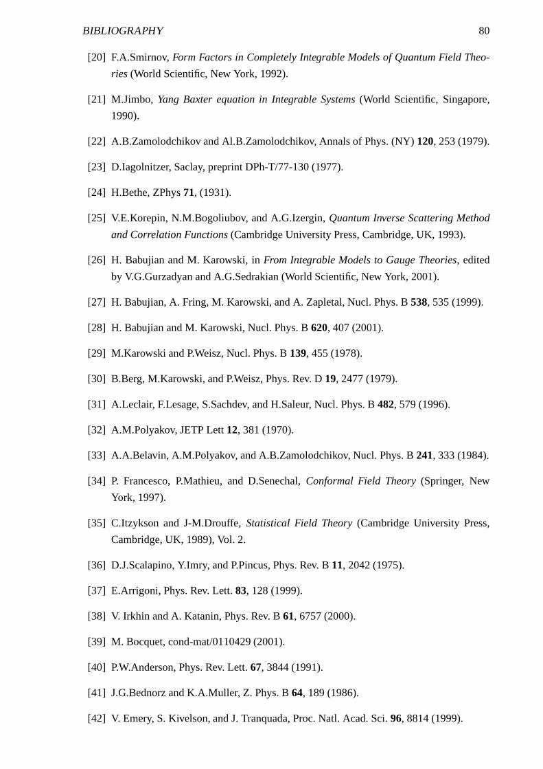
BIBLIOGRAPHY 80
[20] F.A.Smirnov,Form Factors in Completely Integrable Models of Quantum Field Theo-
ries (World Scientific, New York, 1992).
[21] M.Jimbo, Yang Baxter equation in Integrable Systems(World Scientific, Singapore,
1990).
[22] A.B.Zamolodchikov and Al.B.Zamolodchikov, Annals ofPhys. (NY)120, 253 (1979).
[23] D.Iagolnitzer, Saclay, preprint DPh-T/77-130 (1977).
[24] H.Bethe, ZPhys71, (1931).
[25] V.E.Korepin, N.M.Bogoliubov, and A.G.Izergin,Quantum Inverse Scattering Method
and Correlation Functions(Cambridge University Press, Cambridge, UK, 1993).
[26] H. Babujian and M. Karowski, inFrom Integrable Models to Gauge Theories, edited
by V.G.Gurzadyan and A.G.Sedrakian (World Scientific, New York, 2001).
[27] H. Babujian, A. Fring, M. Karowski, and A. Zapletal, Nucl. Phys. B538, 535 (1999).
[28] H. Babujian and M. Karowski, Nucl. Phys. B620, 407 (2001).
[29] M.Karowski and P.Weisz, Nucl. Phys. B139, 455 (1978).
[30] B.Berg, M.Karowski, and P.Weisz, Phys. Rev. D19, 2477 (1979).
[31] A.Leclair, F.Lesage, S.Sachdev, and H.Saleur, Nucl. Phys. B482, 579 (1996).
[32] A.M.Polyakov, JETP Lett12, 381 (1970).
[33] A.A.Belavin, A.M.Polyakov, and A.B.Zamolodchikov, Nucl. Phys. B241, 333 (1984).
[34] P. Francesco, P.Mathieu, and D.Senechal,Conformal Field Theory(Springer, New
York, 1997).
[35] C.Itzykson and J-M.Drouffe,Statistical Field Theory(Cambridge University Press,
Cambridge, UK, 1989), Vol. 2.
[36] D.J.Scalapino, Y.Imry, and P.Pincus, Phys. Rev. B11, 2042 (1975).
[37] E.Arrigoni, Phys. Rev. Lett.83, 128 (1999).
[38] V. Irkhin and A. Katanin, Phys. Rev. B61, 6757 (2000).
[39] M. Bocquet, cond-mat/0110429 (2001).
[40] P.W.Anderson, Phys. Rev. Lett.67, 3844 (1991).
[41] J.G.Bednorz and K.A.Muller, Z. Phys. B64, 189 (1986).
[42] V. Emery, S. Kivelson, and J. Tranquada, Proc. Natl. Acad. Sci.96, 8814 (1999).
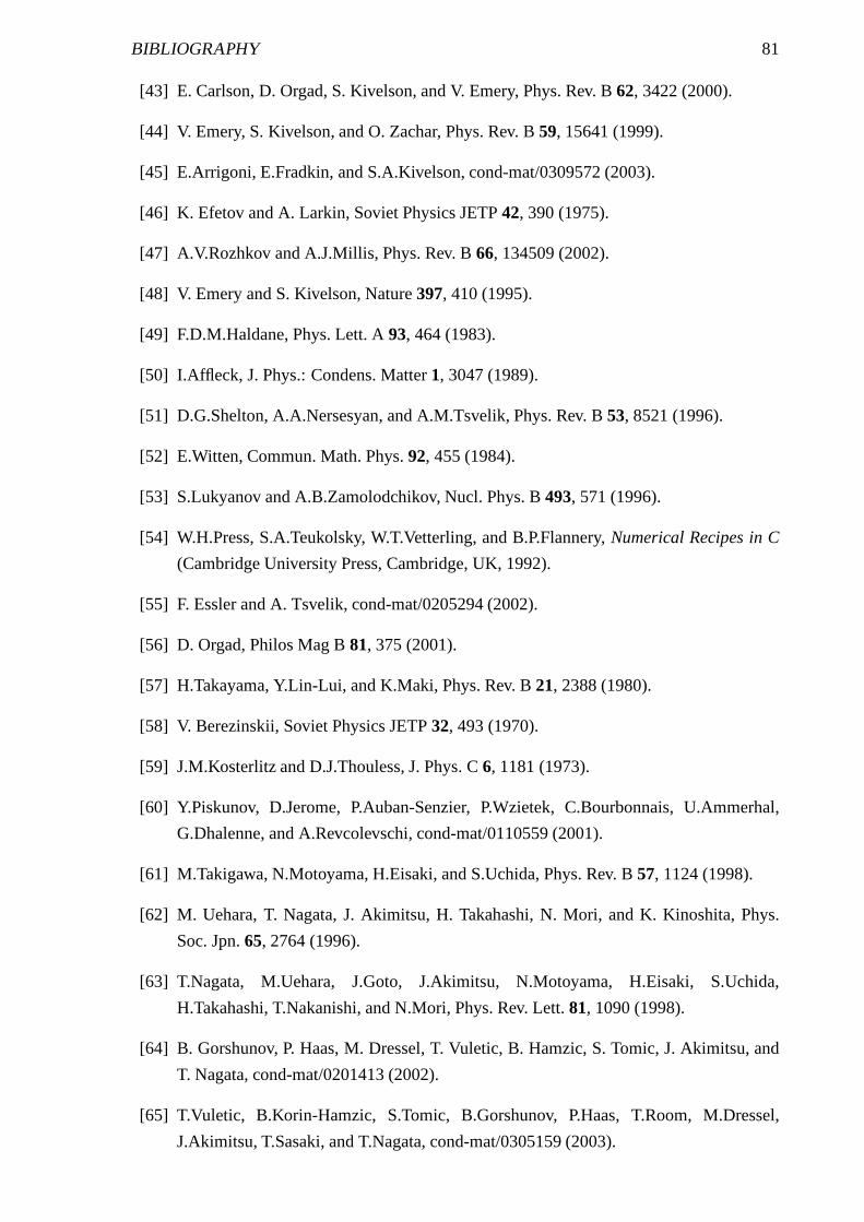
BIBLIOGRAPHY 81
[43] E. Carlson, D. Orgad, S. Kivelson, and V. Emery, Phys. Rev. B 62, 3422 (2000).
[44] V. Emery, S. Kivelson, and O. Zachar, Phys. Rev. B59, 15641 (1999).
[45] E.Arrigoni, E.Fradkin, and S.A.Kivelson, cond-mat/0309572 (2003).
[46] K. Efetov and A. Larkin, Soviet Physics JETP42, 390 (1975).
[47] A.V.Rozhkov and A.J.Millis, Phys. Rev. B66, 134509 (2002).
[48] V. Emery and S. Kivelson, Nature397, 410 (1995).
[49] F.D.M.Haldane, Phys. Lett. A93, 464 (1983).
[50] I.Affleck, J. Phys.: Condens. Matter1, 3047 (1989).
[51] D.G.Shelton, A.A.Nersesyan, and A.M.Tsvelik, Phys. Rev. B53, 8521 (1996).
[52] E.Witten, Commun. Math. Phys.92, 455 (1984).
[53] S.Lukyanov and A.B.Zamolodchikov, Nucl. Phys. B493, 571 (1996).
[54] W.H.Press, S.A.Teukolsky, W.T.Vetterling, and B.P.Flannery,Numerical Recipes in C
(Cambridge University Press, Cambridge, UK, 1992).
[55] F. Essler and A. Tsvelik, cond-mat/0205294 (2002).
[56] D. Orgad, Philos Mag B81, 375 (2001).
[57] H.Takayama, Y.Lin-Lui, and K.Maki, Phys. Rev. B21, 2388 (1980).
[58] V. Berezinskii, Soviet Physics JETP32, 493 (1970).
[59] J.M.Kosterlitz and D.J.Thouless, J. Phys. C6, 1181 (1973).
[60] Y.Piskunov, D.Jerome, P.Auban-Senzier, P.Wzietek, C.Bourbonnais, U.Ammerhal,
G.Dhalenne, and A.Revcolevschi, cond-mat/0110559 (2001).
[61] M.Takigawa, N.Motoyama, H.Eisaki, and S.Uchida, Phys. Rev. B57, 1124 (1998).
[62] M. Uehara, T. Nagata, J. Akimitsu, H. Takahashi, N. Mori, and K. Kinoshita, Phys.
Soc. Jpn.65, 2764 (1996).
[63] T.Nagata, M.Uehara, J.Goto, J.Akimitsu, N.Motoyama,H.Eisaki, S.Uchida,
H.Takahashi, T.Nakanishi, and N.Mori, Phys. Rev. Lett.81, 1090 (1998).
[64] B. Gorshunov, P. Haas, M. Dressel, T. Vuletic, B. Hamzic, S. Tomic, J. Akimitsu, and
T. Nagata, cond-mat/0201413 (2002).
[65] T.Vuletic, B.Korin-Hamzic, S.Tomic, B.Gorshunov, P.Haas, T.Room, M.Dressel,
J.Akimitsu, T.Sasaki, and T.Nagata, cond-mat/0305159 (2003).
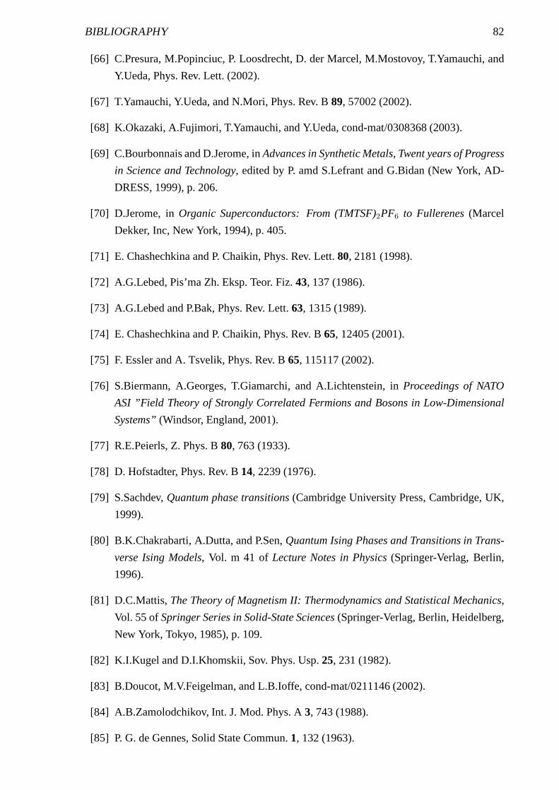
BIBLIOGRAPHY 82
[66] C.Presura, M.Popinciuc, P. Loosdrecht, D. der Marcel,M.Mostovoy, T.Yamauchi, and
Y.Ueda, Phys. Rev. Lett. (2002).
[67] T.Yamauchi, Y.Ueda, and N.Mori, Phys. Rev. B89, 57002 (2002).
[68] K.Okazaki, A.Fujimori, T.Yamauchi, and Y.Ueda, cond-mat/0308368 (2003).
[69] C.Bourbonnais and D.Jerome, inAdvances in Synthetic Metals, Twent years of Progress
in Science and Technology, edited by P. amd S.Lefrant and G.Bidan (New York, AD-
DRESS, 1999), p. 206.
[70] D.Jerome, inOrganic Superconductors: From (TMTSF)2PF6 to Fullerenes(Marcel
Dekker, Inc, New York, 1994), p. 405.
[71] E. Chashechkina and P. Chaikin, Phys. Rev. Lett.80, 2181 (1998).
[72] A.G.Lebed, Pis’ma Zh. Eksp. Teor. Fiz.43, 137 (1986).
[73] A.G.Lebed and P.Bak, Phys. Rev. Lett.63, 1315 (1989).
[74] E. Chashechkina and P. Chaikin, Phys. Rev. B65, 12405 (2001).
[75] F. Essler and A. Tsvelik, Phys. Rev. B65, 115117 (2002).
[76] S.Biermann, A.Georges, T.Giamarchi, and A.Lichtenstein, in Proceedings of NATO
ASI ”Field Theory of Strongly Correlated Fermions and Bosons in Low-Dimensional
Systems”(Windsor, England, 2001).
[77] R.E.Peierls, Z. Phys. B80, 763 (1933).
[78] D. Hofstadter, Phys. Rev. B14, 2239 (1976).
[79] S.Sachdev,Quantum phase transitions(Cambridge University Press, Cambridge, UK,
1999).
[80] B.K.Chakrabarti, A.Dutta, and P.Sen,Quantum Ising Phases and Transitions in Trans-
verse Ising Models, Vol. m 41 of Lecture Notes in Physics(Springer-Verlag, Berlin,
1996).
[81] D.C.Mattis,The Theory of Magnetism II: Thermodynamics and StatisticalMechanics,
Vol. 55 of Springer Series in Solid-State Sciences(Springer-Verlag, Berlin, Heidelberg,
New York, Tokyo, 1985), p. 109.
[82] K.I.Kugel and D.I.Khomskii, Sov. Phys. Usp.25, 231 (1982).
[83] B.Doucot, M.V.Feigelman, and L.B.Ioffe, cond-mat/0211146 (2002).
[84] A.B.Zamolodchikov, Int. J. Mod. Phys. A3, 743 (1988).
[85] P. G. de Gennes, Solid State Commun.1, 132 (1963).
BIBLIOGRAPHY 83
[86] O.Babelon and D.Bernard, Phys. Lett. B288, 113 (1992).
[87] T.T.Wu, B.M.McCoy, C.A.Tracy, and E.Barouch, Phys. Rev. B 13, 316 (1976).
[88] J.Balog and M.Niedermaier, Nucl. Phys. B500, 421 (1997).
[89] G.Delfino and G.Mussardo, Nucl. Phys. B455, 724 (1995).
[90] C.Itzykson and J-M.Drouffe,Statistical Field Theory(Cambridge University Press,
Cambridge, UK, 1989), Vol. 1.
[91] H.J.Schulz and C.Bourbonnais, Phys. Rev. B27, 5856 (1983).
[92] H.J.Schulz, Phys. Rev. Lett.77, 2790 (1996).
[93] V. Fateev, Phys. Lett. B324, 45 (1994).
[94] G. Delfino, G. Mussardo, and P. Simonetti, Nucl. Phys. B473, 469 (1996).
[95] A.Carpy and J.Galy, Acta Crystallogr. Sect B: Struct. Crystallogr. Cryst. Chem.31,
1481 (1975).
[96] M.Isobe and Y.Ueda, J. Phys. Soc. Jpn.65, 1178 (1996).
[97] Y.Fujii, H.Nakao, T.Yoshihama, M.Nishi, K.Nakajima,K.Kakurai, M.Isobe, Y.Ueda,
and H.Sawa, J. Phys. Soc. Jpn.66, 326 (1997).
[98] W.Schnelle, Y.Grin, and R.Kremer, Phys. Rev. B59, 73 (1999).
[99] T.Yosihama, M.Nishi, K.Nakajima, K.Kakurai, Y.Fujii, M.Isobe, C.Kagami, and
Y.Ueda, J. Phys. Soc. Jpn.67, 744 (1998).
[100] A.Meetsma, J. Boer, A.Damascelli, T.T.M.Palstra, J.Jegoudes, and A.Revcolevschi,
Acta. Crysallogr. Sect. C: Cryst. Struct. Commun54, 1558 (1998).
[101] H.Smolinski, C.Gros, W.Weber, U.Peuchert, G.Roth, M.Weiden, and C.Geibel, Phys.
Rev. Lett.80, 5164 (1998).
[102] H.Schnering, Y.Grin, M.Kaupp, M.Somer, R.K.Kremer,O.Jepsen, T.Chatterji, and
M.Weiden, Z.Kristallogr.213, 246 (1998).
[103] A.Bernert, T.Chatterji, P.Thalmeier, and P.Fulde, Euro. Phys. J. B21, 535 (2001).
[104] M.Koppen, D.Pankert, R.Hauptmann, M.Lang, M.weiden, C.Geibel, and F.Steglich,
Phys. Rev. B57, 8466 (1998).
[105] Y.Fagot-Revurat, M.Mehring, and R.Kremer, Phys. Rev. Lett.84, 4176 (2000).
[106] M.V.Mostovoy and D.I.Khomskii, Solid State Commun.113, 159 (2000).
BIBLIOGRAPHY 84
[107] A.Bernert, P.Thalmeier, and P.Fulde, cond-mat/0108008 (2001).
[108] M.V.Mostovoy, D.I.Khomskii, and J.Knoester, Phys. Rev. B65, 64412 (2002).
[109] A.Damascelli, C.Presura, D. der Marel, J.Jegoudez, and A.Revcolevschi, Phys. Rev. B
61, 2535 (2000).
[110] T.D.Schultz, D.C.Mattis, and E.H.Lieb, Rev. Mod. Phys.36, 856 (1964).