Embed Size (px)
Citation preview
HAL Id: hal-01683929https://hal-upec-upem.archives-ouvertes.fr/hal-01683929
Submitted on 15 Jan 2018
HAL is a multi-disciplinary open accessarchive for the deposit and dissemination of sci-entific research documents, whether they are pub-lished or not. The documents may come fromteaching and research institutions in France orabroad, or from public or private research centers.
L’archive ouverte pluridisciplinaire HAL, estdestinée au dépôt et à la diffusion de documentsscientifiques de niveau recherche, publiés ou non,émanant des établissements d’enseignement et derecherche français ou étrangers, des laboratoirespublics ou privés.
Non-Observed Economy vs. the Shadow Economy in theEU: The Accuracy of Measurements Methods and
Estimates revisitedPhilippe Adair
To cite this version:Philippe Adair. Non-Observed Economy vs. the Shadow Economy in the EU: The Accuracy ofMeasurements Methods and Estimates revisited. 4 th OBEGEF Interdisciplinary Insights on Fraudand Corruption , Nov 2017, Porto, Portugal. �hal-01683929�
1
Communication to the 4th OBEGEF Interdisciplinary Insights on Fraud and Corruption
Conference (I2FC2017): ‘The social and economic impact of fraud and corruption’
November 25, Porto, Portugal
Non-Observed Economy vs. the Shadow Economy in the EU:
The Accuracy of Measurements Methods and Estimates revisited
Philippe Adair
Faculty of Economics and Management, ERUDITE, University Paris Est Créteil, France.
Email: [email protected]
Abstract
The Non-Observed Economy (NOE) vs. the shadow economy remains a controversial issue.
Illegal, underground and informal activities encapsulated within the NOE/shadow economy
display large discrepancies throughout the European Union. First, a tractable taxonomy of the
aforementioned market activities is designed according to both definition and scope, whereupon
a wide spectrum of estimation methods applies. Second, direct measurements provided by tax
audits, household informal expenditure and labour market surveys provide piecemeal
information regarding such unobserved activities; a cross-section survey issued from a unique
questionnaire applied to all European countries in 2007 and again in 2013 deserves special
attention. Third, indirect macroeconomic measurements are drawn from discrepancies on the
market for goods and services on the money market and on the labour market, whereas the
DYMIMIC (dynamic multiple indicators-multiple causes) method carves the trends of the
shadow economy (hereafter SE). Fourth, the estimates of the EU shadow economy drawn from
the DYMIMIC model are compared with the assessment of the NOE according to national
accounts adjustments; the relevance of major determinants of the NOE/shadow economy -tax
burden as well as the characteristics of the informal workforce, is discussed.
Keywords: Estimates; European Union; Measurement Methods; National Accounts; Shadow
Economy.
JEL: C18, E1, H26, K42, O52
2
1. Issues
Since the first report for the European Commission (Barthélémy et al, 1990), the European
Union (hereafter EU) initiated several studies upon undeclared economic activities, which
escape social regulations and tax compliance as well as statistical recording. The topic has been
expanding throughout the late 1970s; since then, experts loosely used various terms as
synonyms to capture these activities e.g. “black, concealed, hidden, informal, irregular, non-
observed, shadow, subterranean, underground, unofficial, unrecorded”, etc (Feige, 1989;
Thomas, 1992; The Economic Journal, 1999; Schneider and Enste, 2000).
However, definition and scope differ among scholars, as well as the magnitude and trends
according to measurement methods. The path towards a tractable taxonomy remains work in
progress, although major steps have been achieved in the past decades. The ILO (1993)
provided guidelines for statistics on the informal sector and enlarged the scope towards informal
employment (ILO, 2002), which became part of the Manuel on the informal economy (ILO,
2013). Alongside OECD and the IMF, the ILO co-authored the Handbook for Measurement of
the Non-Observed Economy (OECD, 2002), which coined the Non-Observed Economy
(hereafter NOE) from the United Nations System of National Accounts (SNA) perspective. The
United Nations Economic Commission for Europe launched two surveys on national practices
regarding the NOE in national accounts (UNECE, 2003, 2008). The SNA was revised in 2008,
the revision of which was transposed into the European System of Accounts (ESA) in 2010 and
the Eurostat national accounts update include some components of the NOE in 2014.
Meanwhile, Schneider and Williams (2013), Schneider (2015) and Schneider et al. (2015)
provided extensive updates of the “shadow economy” (hereafter SE) estimates based upon a
calibrated structural model (DYMIMIC), while other scholars used Dynamic General
Equilibrium (DGE) models that reached similar magnitude and trends of the SE (Elgin and
Schneider, 2016). National accountants (Ven, 2017) and Feige (2015) dismissed such so-called
“black box modelling” upon the SE as inaccurate and overstated. Indeed the topic of NOE vs.
SE is controversial. How should the NOE/SE be accounted for? How large or small a share of
GDP does it represent in the EU countries? Are the trends declining since the 1990s?
Section 2 is devoted to definition and scope: NOE is designed as a set of eight types or seven
categories of activities liable to taxes that are encapsulated within five categories: Illegal
economy, underground economy and the informal economy are market activities, whereas
production for own final use is non-market output.
3
Section 3 examines the spectrum of definitions and estimation methods, both direct and indirect.
Seven different methods fall into two broad categories. It first presents direct measurements
provided by tax audits, household informal expenditure surveys and labour market surveys; a
special attention is paid to the cross-section survey issued from a unique questionnaire applied
to all European countries in 2007 and repeated in 2013.
Section 4 deals with indirect macroeconomic measurements that are drawn from discrepancies
between income and expenditure on the commodity market, discrepancies on the money market
and discrepancies on the labour market, as well as from non-monetary (i.e. qualitative)
modelling of latent variables and multiple indicators-multiple causes (MIMIC).
Section 5 compares the estimates of the NOE from EU national accounts with those of the SE
drawn from the DYMIMIC model; it discusses the impact of some major determinants such as
tax pressure and the informal workforce.
Section 6 briefly recapitulates the strengths and weaknesses of both methods and sketches a
research agenda.
2. Non-Observed Economy and the Shadow Economy: Definition and Scope.
2.1. The components of NOE.
NOE, a useful typology albeit not an analytical classification, is the outcome of an ongoing
process of extensive coverage upon productive activities, in order to design an exhaustive
standardized definition for measuring concealed GDP.
National accountants have traditionally sought to incorporate undeclared production, incomes
and expenditures by reconciling income, expenditure and output estimates of GDP. According
to international principles of national accounting, GDP includes all types of value added in the
economy as evidenced by voluntary transactions where payments are made, including illegal
and barter transactions. GDP also includes some production without transactions such as
imputed rents and household production for own use. The first and most important distinction
must be drawn between market traded and non-market traded goods and services, both being
included in the GDP. The second distinction concerns the compliance with legal standards:
illegal activities are criminal, whereas other unobserved activities are legal. A third distinction
relates to the nature of the flow: according to the value added approach of GDP, activities that
produce an output are included, whereas income transfers (pilfering, theft extortion or money
laundering) are not. According to the current nomenclature from Eurostat tabular approach, the
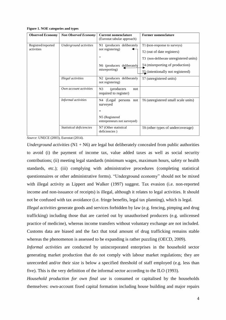
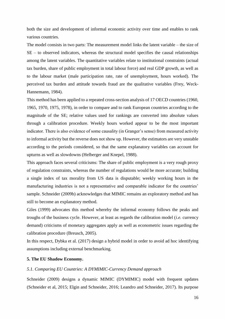
NOE comprises five broad categories of activities, namely Underground, Illegal, Own-account,
Informal, and Statistical deficiencies. (See Figure 1).
4
Figure 1. NOE categories and types
Observed Economy Non Observed Economy Current nomenclature
(Eurostat tabular approach) Former nomenclature
Registred/reported
activities
Underground activities N1 (producers deliberately
not registering)
+
N6 (producers deliberately
misreporting)
T1 (non-response to surveys)
T2 (out of date registers)
T3 (non-deliberate unregistered units)
T4 (misreporting of production)
T5 (intentionally not registered)
Illegal activities N2 (producers deliberately
not registering) T7 (unregistered units)
Own account activities N3 (producers not
required to register)
Informal activities N4 (Legal persons not
surveyed
+
N5 (Registered
entrepreneurs not surveyed)
T6 (unregistered small scale units)
Statistical deficiencies N7 (Other statistical
deficiencies ) T8 (other types of undercoverage)
Source: UNECE (2003), Eurostat (2014).
Underground activities (N1 + N6) are legal but deliberately concealed from public authorities
to avoid (i) the payment of income tax, value added taxes as well as social security
contributions; (ii) meeting legal standards (minimum wages, maximum hours, safety or health
standards, etc.); (iii) complying with administrative procedures (completing statistical
questionnaires or other administrative forms). “Underground economy” should not be mixed
with illegal activity as Lippert and Walker (1997) suggest. Tax evasion (i.e. non-reported
income and non-issuance of receipts) is illegal, although it relates to legal activities. It should
not be confused with tax avoidance (i.e. fringe benefits, legal tax planning), which is legal.
Illegal activities generate goods and services forbidden by law (e.g. fencing, pimping and drug
trafficking) including those that are carried out by unauthorised producers (e.g. unlicensed
practice of medicine), whereas income transfers without voluntary exchange are not included.
Customs data are biased and the fact that total amount of drug trafficking remains stable
whereas the phenomenon is assessed to be expanding is rather puzzling (OECD, 2009).
Informal activities are conducted by unincorporated enterprises in the household sector
generating market production that do not comply with labour market regulations; they are
unrecorded and/or their size is below a specified threshold of staff employed (e.g. less than
five). This is the very definition of the informal sector according to the ILO (1993).
Household production for own final use is consumed or capitalised by the households
themselves: own-account fixed capital formation including house building and major repairs
5
(owner imputed rents) and services of paid domestic servants. Do It Yourself (DIY) home
repairs and improvements range from 1% to 3% of GDP in Denmark, Sweden, Germany and
the United Kingdom (OECD, 2004); a part of which is included in the GDP. Barter and in-kind
exchanges between households are unregistered and not liable to tax should also be included.
2.2. Coverage of the NOE in the EU: the long road to exhaustiveness.
As Blades and Robert (2002) put it, non-observed does not mean non accounted activities:
National Accounts do adjust for various types of NOE; thus the ratio of NOE to GDP is
meaningful and should comply with the European statistical framework (Eurostat).
A tentative measurement of NOE in OECD countries was set up in the 1980s as regards tax
evasion and undeclared work, misappropriated in kind incomes and production of illegal goods
and services: Figures amounted from 2 up to 5% of GDP in the 1970s (Blades, 1982).
A second survey in 2001-2002 (UNECE, 2003) covered 16 European countries: six from the
EU and nine candidate countries, plus Croatia. The methods enhancing exhaustiveness in the
national accounts capture informal and underground activities, although it may not be possible
to identify and classify them separately in most EU countries, Italy been excepted.
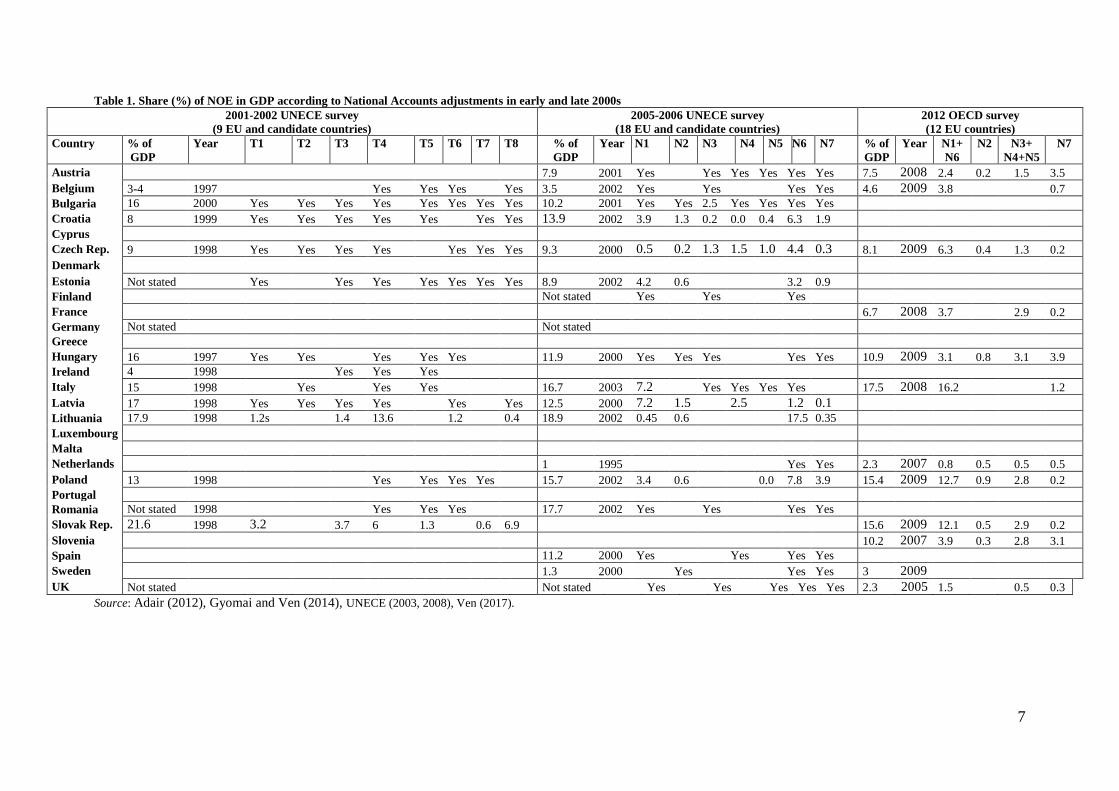
In 2005-2006 A third survey (UNECE, 2008) enlarged the sample to 18 countries (17 EU
Members States plus Croatia) and the new nomenclature of NOE activities applied (See Figure
1). Neither coverage nor dates do match due to a different scheduling across countries as well
as to the non-binding requirement of such surveys. Countries with the largest coverage display
the highest NOE magnitude; conversely, countries with the smallest coverage display the lowest
NOE magnitude. A comparison between countries providing NOE estimates for the previous
survey shows that trends remain stable in Belgium, whereas they decline (Bulgaria, Hungary
and Latvia) or increase (Czech Republic, Italy, Lithuania and Poland). This could be due to the
change in nomenclature but not necessarily to the improvement in coverage as for the
complying Eastern European countries. As for Belgium, one may suspect that adjustments use
the same parameters; therefore, it is no surprise that the NOE remains stable (See Table 1).
In 2012, the OECD used the same nomenclature to survey 12 countries (Gyomai and Ven, 2014;
Ven, 2017), out of which six were already included in the 2005-2006 survey (UNECE, 2008).
Trends decline (Austria, Czech Republic, Hungary and Poland) or increase (Belgium, Italy,
Netherlands and Sweden), mostly because coverage improved.
Despite the agreement of EU countries as regards compliance with the European System of
Accounts (ESA 2010), the adjustment process in order to include the NOE experienced slow
completion. In 2014, Eurostat required that N2 be included in the GDP for 2010 and it would
6
slightly increase the share of NOE in the GDP for most countries. However, coverage remains
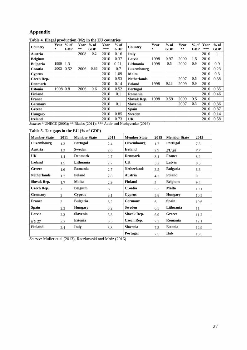
disparate and a few countries prove reluctant to disclosure (See Table 4 in the appendix).
7
Table 1. Share (%) of NOE in GDP according to National Accounts adjustments in early and late 2000s
2001-2002 UNECE survey
(9 EU and candidate countries)
2005-2006 UNECE survey
(18 EU and candidate countries)
2012 OECD survey
(12 EU countries)
Country
% of
GDP
Year
T1
T2
T3
T4
T5
T6
T7
T8
% of
GDP
Year
N1
N2
N3
N4
N5
N6
N7
% of
GDP
Year N1+
N6
N2 N3+
N4+N5
N7
Austria 7.9 2001 Yes Yes Yes Yes Yes Yes 7.5 2008 2.4 0.2 1.5 3.5
Belgium 3-4 1997 Yes Yes Yes Yes 3.5 2002 Yes Yes Yes Yes 4.6 2009 3.8 0.7
Bulgaria 16 2000 Yes Yes Yes Yes Yes Yes Yes Yes 10.2 2001 Yes Yes 2.5 Yes Yes Yes Yes
Croatia 8 1999 Yes Yes Yes Yes Yes Yes Yes 13.9 2002 3.9 1.3 0.2 0.0 0.4 6.3 1.9
Cyprus
Czech Rep. 9 1998 Yes Yes Yes Yes Yes Yes Yes 9.3 2000 0.5 0.2 1.3 1.5 1.0 4.4 0.3 8.1 2009 6.3 0.4 1.3 0.2
Denmark
Estonia Not stated Yes Yes Yes Yes Yes Yes Yes 8.9 2002 4.2 0.6 3.2 0.9
Finland Not stated Yes Yes Yes
France 6.7 2008 3.7 2.9 0.2
Germany Not stated Not stated
Greece
Hungary 16 1997 Yes Yes Yes Yes Yes 11.9 2000 Yes Yes Yes Yes Yes 10.9 2009 3.1 0.8 3.1 3.9
Ireland 4 1998 Yes Yes Yes
Italy 15 1998 Yes Yes Yes 16.7 2003 7.2 Yes Yes Yes Yes 17.5 2008 16.2 1.2
Latvia 17 1998 Yes Yes Yes Yes Yes Yes 12.5 2000 7.2 1.5 2.5 1.2 0.1
Lithuania 17.9 1998 1.2s 1.4 13.6 1.2 0.4 18.9 2002 0.45 0.6 17.5 0.35
Luxembourg
Malta
Netherlands 1 1995 Yes Yes 2.3 2007 0.8 0.5 0.5 0.5
Poland 13 1998 Yes Yes Yes Yes 15.7 2002 3.4 0.6 0.0 7.8 3.9 15.4 2009 12.7 0.9 2.8 0.2
Portugal
Romania Not stated 1998 Yes Yes Yes 17.7 2002 Yes Yes Yes Yes
Slovak Rep. 21.6 1998 3.2 3.7 6 1.3 0.6 6.9 15.6 2009 12.1 0.5 2.9 0.2
Slovenia 10.2 2007 3.9 0.3 2.8 3.1
Spain 11.2 2000 Yes Yes Yes Yes
Sweden 1.3 2000 Yes Yes Yes 3 2009
UK Not stated Not stated Yes Yes Yes Yes Yes 2.3 2005 1.5 0.5 0.3
Source: Adair (2012), Gyomai and Ven (2014), UNECE (2003, 2008), Ven (2017).
8
3. Measurement Methods and Estimates: Three Direct Approaches.
Direct investigations are provided by tax audits, household expenditure surveys and labour
market surveys. They are used in order to collect raw data or control the various estimates
computed through indirect approaches.
3.1. Tax Audits
Audits investigating tax compliance focus on targeted sub samples that are not representative
of the population. They cannot collect data on illegal activities. They provide point estimates
rather than time series data. Indirect detection controlled estimations are based on
characteristics of potential offenders, providing both the estimates of the probability of
compliance vs. violation (by means of maximum likelihood) and the proportion of violations
remaining undetected (applying Bayes’ law). However, violation and detection prove uneasy
to disentangle. Surveys underestimate the size of the SE (Giles 1999; Schneider and Enste
2000). The same comments apply to social security contributions. In this connection,
administrative data and findings from labour inspectorates may be useful, but international
comparisons based primarily on these sources have not taken place yet.
3.2. Households’ expenditure and labour market: the 2007 and 2013 Eurobarometers.
Sparse households’ expenditure surveys have been carried on the relevant assumption that it is
easier to collect data from the customers on the demand side than from those who provide their
provisioning on the supply side.
As regards the labour market surveys, the Labour Force Survey designed by Eurostat does not
address informal employment. However, a few surveys were undertaken in the 1980s by
Statistical Offices (Italy, Netherlands and Spain) and NGOss (Germany and Norway),
displaying a large difference between Northern and Southern European countries (OECD,
2004).
Box: the Rockwool Foundation pilot survey on undeclared work
At the start of the millennium, comparable surveys conducted with the same questionnaires by the Rockwool
Foundation in Northern Europe find that “black” hours worked are just over 1% in Great Britain, 2-3% in Sweden
and about 4% in Denmark and Germany. Estimates seem to have slightly increased overtime as regards Denmark
and Germany. Percentages of GDP when informal work is valued at the actual prices paid by purchasers are lower
than when it is valued at formal prices; the former measurement seems quite realistic. On the one hand, there is a
lack in coverage for non-wage payments; on the other hand, wages are valued according to average legal wages
whereas a valuation according to average wages paid for informal employees would cut off the magnitude to less
than half of the official figures.
9
Inspiring from the Rockwool Foundation methodology (See box), the first European survey on
a stratified households sample in each of the 27 EU countries took place in 2007 and was
repeated in 2013 (EEC, 2007; 2013), providing a comprehensive basis for comparison. Both
Eurobarometers address household expenditure on informal goods and services, undeclared
work (or informal employment according to ILO) and attitude towards fraud; criminal activities
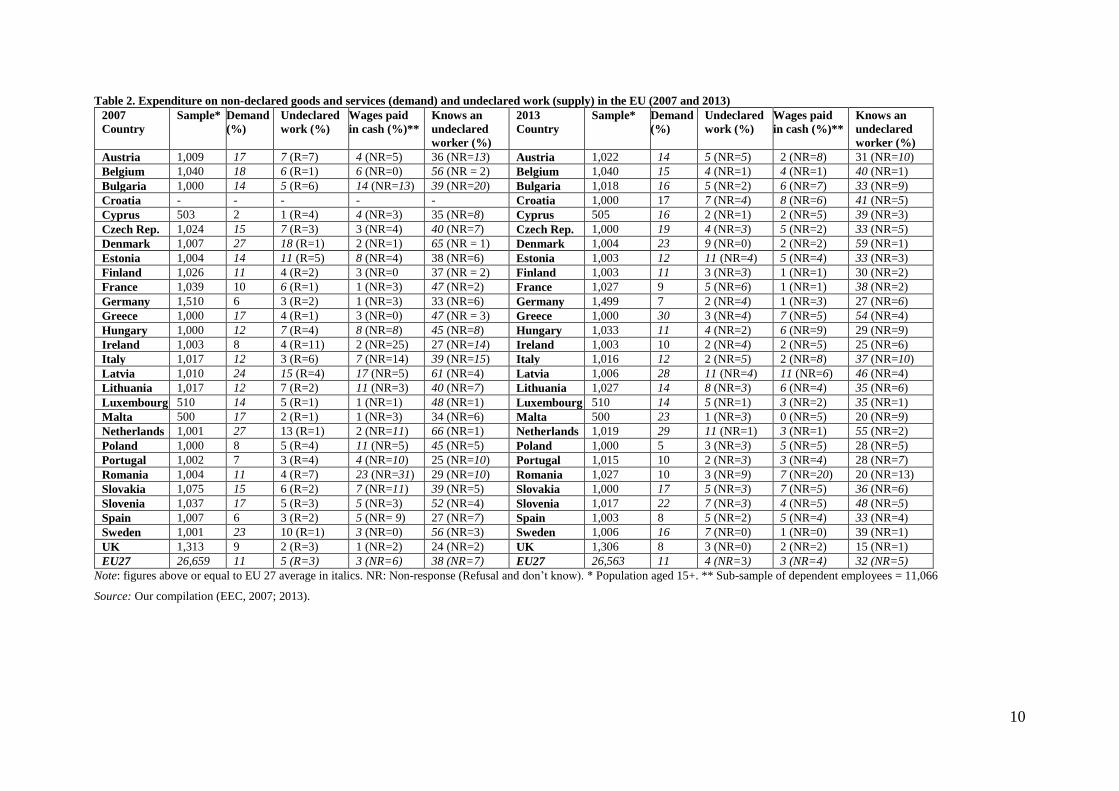
and sub-contracting were not investigated (See Table 2).
The demand for non-declared goods and above all for services comes from rather young (below
40 years old) and well educated customers. Supply is provided by local networks (neighbours,
family and friends) in two cases out of five and by self-employed and firms in one case out of
five. Lower prices as compared to official provisioning is the main drive in two thirds of cases
but purchase is no related to prices in one case out of four and this should be explained.
On the demand side, purchasers of non-declared goods and services are usually in higher
numbers than those who perform undeclared work, and there is a weak correlation between
these two categories.
Undeclared work is paid for in two cases out of three; it is performed by males (twice as many
as females), respectively on a regular or periodical basis in half and one third of cases, at most
during five weeks a year on average in households services, construction and manufacturing
industries.
Cash payments for (“envelope”) wages are widespread in Eastern Europe, enabling businesses
to save on tax and social security contributions; there is a high rate of non-response for most
countries, and the sub-sample is not representative.
Undeclared work or cash payments are not widespread as compared with the share of
interviewees who know an undeclared worker; one may suspect that undeclared work is
understated in most countries wherein the rate of non-response tops EU 27 average. It is rather
unfortunate that Kayaoglu and Williams (2017) focus on dependent employees (envelope
wages), who are only a fraction of informal employment issue they address.
Attitude (morale) towards fraud is computed with a non weighted score scaling from 1 (no
tolerance) up to 10 (tolerance without restriction), as regards 5 questions related to fraud on
social security (households and firms), non-tax reporting, fraud on social benefits- and fraud in
public transportation.
These methods provide biased estimates in as much as respondents may understate their job
status. Also, it unlikely that such surveys will be used frequently implemented and provide time
series.
10
Table 2. Expenditure on non-declared goods and services (demand) and undeclared work (supply) in the EU (2007 and 2013)
2007
Country
Sample* Demand
(%)
Undeclared
work (%)
Wages paid
in cash (%)**
Knows an
undeclared
worker (%)
2013
Country
Sample* Demand
(%)
Undeclared
work (%)
Wages paid
in cash (%)**
Knows an
undeclared
worker (%)
Austria 1,009 17 7 (R=7) 4 (NR=5) 36 (NR=13) Austria 1,022 14 5 (NR=5) 2 (NR=8) 31 (NR=10)
Belgium 1,040 18 6 (R=1) 6 (NR=0) 56 (NR = 2) Belgium 1,040 15 4 (NR=1) 4 (NR=1) 40 (NR=1)
Bulgaria 1,000 14 5 (R=6) 14 (NR=13) 39 (NR=20) Bulgaria 1,018 16 5 (NR=2) 6 (NR=7) 33 (NR=9)
Croatia - - - - - Croatia 1,000 17 7 (NR=4) 8 (NR=6) 41 (NR=5)
Cyprus 503 2 1 (R=4) 4 (NR=3) 35 (NR=8) Cyprus 505 16 2 (NR=1) 2 (NR=5) 39 (NR=3)
Czech Rep. 1,024 15 7 (R=3) 3 (NR=4) 40 (NR=7) Czech Rep. 1,000 19 4 (NR=3) 5 (NR=2) 33 (NR=5)
Denmark 1,007 27 18 (R=1) 2 (NR=1) 65 (NR = 1) Denmark 1,004 23 9 (NR=0) 2 (NR=2) 59 (NR=1)
Estonia 1,004 14 11 (R=5) 8 (NR=4) 38 (NR=6) Estonia 1,003 12 11 (NR=4) 5 (NR=4) 33 (NR=3)
Finland 1,026 11 4 (R=2) 3 (NR=0 37 (NR = 2) Finland 1,003 11 3 (NR=3) 1 (NR=1) 30 (NR=2)
France 1,039 10 6 (R=1) 1 (NR=3) 47 (NR=2) France 1,027 9 5 (NR=6) 1 (NR=1) 38 (NR=2)
Germany 1,510 6 3 (R=2) 1 (NR=3) 33 (NR=6) Germany 1,499 7 2 (NR=4) 1 (NR=3) 27 (NR=6)
Greece 1,000 17 4 (R=1) 3 (NR=0) 47 (NR = 3) Greece 1,000 30 3 (NR=4) 7 (NR=5) 54 (NR=4)
Hungary 1,000 12 7 (R=4) 8 (NR=8) 45 (NR=8) Hungary 1,033 11 4 (NR=2) 6 (NR=9) 29 (NR=9)
Ireland 1,003 8 4 (R=11) 2 (NR=25) 27 (NR=14) Ireland 1,003 10 2 (NR=4) 2 (NR=5) 25 (NR=6)
Italy 1,017 12 3 (R=6) 7 (NR=14) 39 (NR=15) Italy 1,016 12 2 (NR=5) 2 (NR=8) 37 (NR=10)
Latvia 1,010 24 15 (R=4) 17 (NR=5) 61 (NR=4) Latvia 1,006 28 11 (NR=4) 11 (NR=6) 46 (NR=4)
Lithuania 1,017 12 7 (R=2) 11 (NR=3) 40 (NR=7) Lithuania 1,027 14 8 (NR=3) 6 (NR=4) 35 (NR=6)
Luxembourg 510 14 5 (R=1) 1 (NR=1) 48 (NR=1) Luxembourg 510 14 5 (NR=1) 3 (NR=2) 35 (NR=1)
Malta 500 17 2 (R=1) 1 (NR=3) 34 (NR=6) Malta 500 23 1 (NR=3) 0 (NR=5) 20 (NR=9)
Netherlands 1,001 27 13 (R=1) 2 (NR=11) 66 (NR=1) Netherlands 1,019 29 11 (NR=1) 3 (NR=1) 55 (NR=2)
Poland 1,000 8 5 (R=4) 11 (NR=5) 45 (NR=5) Poland 1,000 5 3 (NR=3) 5 (NR=5) 28 (NR=5)
Portugal 1,002 7 3 (R=4) 4 (NR=10) 25 (NR=10) Portugal 1,015 10 2 (NR=3) 3 (NR=4) 28 (NR=7)
Romania 1,004 11 4 (R=7) 23 (NR=31) 29 (NR=10) Romania 1,027 10 3 (NR=9) 7 (NR=20) 20 (NR=13)
Slovakia 1,075 15 6 (R=2) 7 (NR=11) 39 (NR=5) Slovakia 1,000 17 5 (NR=3) 7 (NR=5) 36 (NR=6)
Slovenia 1,037 17 5 (R=3) 5 (NR=3) 52 (NR=4) Slovenia 1,017 22 7 (NR=3) 4 (NR=5) 48 (NR=5)
Spain 1,007 6 3 (R=2) 5 (NR= 9) 27 (NR=7) Spain 1,003 8 5 (NR=2) 5 (NR=4) 33 (NR=4)
Sweden 1,001 23 10 (R=1) 3 (NR=0) 56 (NR=3) Sweden 1,006 16 7 (NR=0) 1 (NR=0) 39 (NR=1)
UK 1,313 9 2 (R=3) 1 (NR=2) 24 (NR=2) UK 1,306 8 3 (NR=0) 2 (NR=2) 15 (NR=1)
EU27 26,659 11 5 (R=3) 3 (NR=6) 38 (NR=7) EU27 26,563 11 4 (NR=3) 3 (NR=4) 32 (NR=5)
Note: figures above or equal to EU 27 average in italics. NR: Non-response (Refusal and don’t know). * Population aged 15+. ** Sub-sample of dependent employees = 11,066
Source: Our compilation (EEC, 2007; 2013).
11
4. Measurement Methods and Estimates: Indirect Approaches.
Indirect macroeconomic measurements are drawn from discrepancies between income and
expenditure on the commodity market, discrepancies on the money market and discrepancies
on the labour market, as well as from qualitative non-monetary modelling of latent variables
and multiple indicators-multiple causes models using monetary calibration (DYMIMIC).
4.1. Discrepancies between income and expenditure on the market for goods and services.
By definition, the income approach of GDP should reach the same outcome as the expenditure
approach; hence, any discrepancy such as income being larger than expenditure, indicates the
existence of a ‘hidden’ economy (excluding criminal activities). Several European countries
investigated the income-expenditure gap, among which the UK has documented this gap, due
to tax evasion, relying on household living standards surveys. According to restricted or
extensive assumptions, the range of estimates varies from less than 3% up to over 10% of GDP.
This method covers only the “underground economy” NOE type.
Dilnot and Morris (1981) use a disaggregated analysis which examines both the income and
expenditure behaviour of a sample of 1,000 households drawn from the UK Family Expenditure
Survey (FES) and then extend the analysis to the whole FES sample of 7,200 households in
order to track ‘black’ economic activity (including tax evasion and social security fraud). After
correcting the data for deficiencies and relying on a sample of households whose expenditure
exceeds 1.15 of their reported income, the estimate ranges between 2.3% and 3% of GDP
(1977). The main drawback is the assumption that the FES is a reliable source of information,
despite the fact that the rate of non-response is 30%; actually, the “black economy” is
underrated, because self-employment is under-reported in the FES.
Pissarides and Weber (1989) use a food consumption function to estimate the size of the black
economy from the FES, assuming that only self-employed underreport their income. The
estimates for underreporting amounts to 5.5% of GDP (1982). This method has several
shortcomings: Some employees may engage in self-employment and conceal their income. The
relevant assumption that food expenditure is more accurately recorded than other items of
expenditure overlooks the fact that luxury items of expenditures (including food) may be
underreported. Savings are not taken into account. Preferences are assumed to be identical,
whatever the households’ characteristics may be.
Lyssiotou et al (2004) use a single equation for a complete demand system encompassing six
categories of non-durable goods. It is based on cross-section individual household data from
the FES, and includes both wages and self-employment incomes. It avoids the confusion
12
between preference heterogeneity and income effects, and takes into account the household
characteristics to calibrate the size of the black economy in the UK amounting 10.6% of GDP
(1989). The model does not reach a complete demand system; pensioners and single parents are
excluded from the sample; the preferences of self-employed are rather peculiar.
Estimates based on discrepancies between income and expenditure, whatever the methods used,
capture only a part of NOE and face several shortcomings. On the one hand, statistical offices
may be prone to political influence; there are incentives for higher estimates when the country
is a large tax burden and lower estimates when experiencing financial assistance (Tanzi, 1999).
Measurement is inadequate because Income and Expenditure are not estimated according to
independent sources (Barthélémy, 1988; Feige, 1989; Thomas, 1992). On the other hand,
missing income and non-reported revenue may not be linked. In addition, tax evaded income
maybe overestimated due to the fact that the level of earnings of the informal workers could be
too low to pay taxes (Bhattacharyya, 1999).
4.2. Discrepancies regarding monetary aggregates on the money market
Monetary measures can be classified into two categories: the currency ratio/ demand method
and the transactions method.
4.2.1. Currency ratio/demand method
The method pioneered by Gutmann (1985) does not use any statistical analysis, but simply
disentangles the money supply, M1, into two components, currency and demand deposits, and
examines their movement as well as the ratio of currency to deposits over the period 1937-76.
He assumes that non-declared transactions are paid in cash, and that the velocity of circulation
is the same in both the formal and ‘underground’ economies; he takes into account the variation
of the cash/deposits (C/D) ratio according to the basic period (or year) considered as an indicator
of the ‘underground’ economy.
The currency demand approach pioneered by Cagan (1958) is advocated by Tanzi (1982). Tanzi
assumes that economic agents involve in ‘underground’ activities in order to escape taxes; thus
an estimate of the tax elasticity of currency demand can be used to calculate the stock of
currency held in the underground economy. Provided that the income velocity of money in the
underground economy is the same as that in the legal economy, then the size of the former can
be approximated by multiplying the income velocity of money in the legal economy by the
stock of money in the underground economy.
Tanzi (1982) runs a simple econometric equation on US time-series data for the period 1929-
76. The dependent variable is the ratio of currency to deposits, using M2 as the measure of
13
money supply. Other independent variables are per capita income, the ratio of total wages and
salaries in personal income, and the rate of interest on time deposits as a measure of the
opportunity cost of holding cash. The currency ratio is negatively related to per capita income,
whereas the ratio of total wages and salaries (paid in cash) is positively related to the currency
ratio. The connection between changes in the level of income taxes and changes in the C /M2
ratio is imputed to the ‘underground’ economy.
The currency demand approach has been criticised on three grounds (Thomas, 1999). A base
year or period is needed, but the assumption of a period during which there was no informal
activity is absurd. The assumption that the velocity of circulation is the same in both the official
and informal economies requires some explanation. The assumption that transactions are
carried out in cash only is unrealistic. Hence, Tanzi’s econometric model is misspecified and
proves unstable.
4.2.2 Transactions method
The monetary transactions method developed by Feige (1989) takes Fisher’s equation of
exchange as a starting point and assumes that transactions are paid in cash as well as in cheques;
he attributes the underground economy to the discrepancy between independent estimates of
MV and PT (which includes both formal and informal transactions). Following the Cambridge
equation of exchange, total income is computed from recorded and unrecorded income: In order
to estimate unrecorded income, Feige assumes that there was a period (i.e. a benchmark year)
during which all income was properly recorded.
If the assumption that non-declared transactions are not exclusively paid in cash seems realistic,
it may also over-estimate the extent of these transactions, since cheques are also used to carry
out transfers without relationship with non-declared transactions.
Feige’s method has been criticised because its estimates are sensitive to the choice of initial
period (Tanzi, 1982) and lack empirical validity (Thomas, 1992).
All monetary approaches provide, in absolute value, a large spectrum of estimates in terms of
GDP: Feige’s ratio is increasingly higher than Gutmann’s ratio which in turn is higher than
Tanzi’s ratio. In terms of logarithms, they seem to show either a growing trend (currency
demand) or cycles which converge or diverge according to countries (cash ratio, transactions)
(Schneider and Enste, 2000).
Despite several restrictions they point out, Schneider and Enste (2000) and Schneider (2015,
2016) use extensively the Cagan-Tanzi currency demand approach to calibrate the DYMIMIC
model. The main reason seems to be that, due to the availability of time series data, estimates
14
provide trends and enable cross-section comparisons. However, the model should not apply to
short-run data: According to Ahumada et al. (2008), in order to avoid the problem of initial
condition (or benchmark), the model should only be designed and computed to account for long
run trends.
All monetary models eschew economic theory as regards behaviour on the money market,
especially preferences relating to the various ways whereby currency is used and kept (species,
current accounts), which can vary according to the institutional framework and periods
considered. Savings or currency hoarding are not taken into account (Thomas, 1999), possibly
causing an overestimation or, in case of previous hoarding, causing an underestimation of the
hidden economy; Bhattacharyya (1999) assumes that these two opposite forces cancel
themselves but provides no evidence. According to Giles (1999) monetary approaches
overestimate the size of the SE.
4.3. Discrepancies on the labour market
Contini (1981) examines the growth of the “irregular labour market” (i.e. jobs outside the social
security system) in Italy during the 1960s and 1970s, which is due to three factors: The labour
supply is driven by the preference of workers for flexibility in their allocation of time as well
as the avoidance of unemployment, the labour demand from small-scale enterprises for workers
prepared to earn less than on the regular labour market, tax evasion by employers in the form
of the non-payment of payroll taxes and indirect charges (50% -70% to the basic pay) given the
existence of strict job protection legislation. Contini’s estimates of the size of the irregular
labour force reach 16% - 18% of the total labour force in the late 1970s. Given the fact that high
levels of unemployment seem to be in pace with the underground economy, the deficiency
within employment estimates or the so-called ‘implicit labour supply’ fills the gap between
official labour force participation and the effective labour force participation measured through
various investigations, surveys and computations. The official labour force is thus raised by a
coefficient resulting from the conversion of the multiple job holding and non-declared activity
into full-time employment. Then, it is multiplied by the value added per unit of employment
(VAPUE) in order to compute the missing output. Italy carried out the calculation of implicit
labour supply, which reached 17.7% of GDP in 1987 and was officially included within national
accounts.
Such a method faces two major drawbacks. On the one hand, the official definition of the labour
force (according to ILO) does not include either children or retired people in the informal work
force, which will then be underestimated. On the other hand, the World Bank (2007) points out
15
that the distinction between the formal and informal labour market is blurred. On the other hand,
the basic assumption, which in turn leads to an overestimation, is that the VAPUE in the
underground economy is the same as in the official economy: There are reasons to believe that
the VAPUE of the former is weaker than in the latter, since most workers in the informal
economy have less human capital and/or equipment, thus yielding a lower productivity (Tanzi,
1999). However, Giles (1999) and Schneider and Enste (2000) contend that labour force
participation data are biased and underestimate the size of the informal economy.
4.4. Estimates from real and monetary modelling
Most macro-economic methods are based on one indicator – currency demand, electricity
consumption or unreported labour activity – in order to capture the overall NOE; thus the
estimate takes into account only one among its several components.
4.4.1. Electricity consumption methods
The rationale for electricity consumption assumes it is a good proxy for both official and
unofficial economic activities, and the methods provide time series data that has been used by
East European countries before joining the EU. Kaufmann and Kaliberda (1996) derive an
estimate of unrecorded GDP from the difference between the growth of official GDP and the
growth of the overall use of electricity. Lackó (2000) takes into account the households
activities, which include DIY and home production, thus allowing a broader scope and
providing higher estimates. Unfortunately, the size of the SE is exogenous and remains
unexplained. Both methods can be criticised on two points: all unofficial activities do not
require extra electricity consumption (e.g. street trading); variations in the elasticity of
electricity/GDP do occur and are due to factors that may not be related to unofficial activities
of the households and the firms.
Although it displays a flatter trend than monetary methods and, electricity consumption method
overstates NOE in comparison with national accounts estimates (UNECE, 2003)
However, strangely enough, Medina and Schneider (2017) use light intensity as a calibration
method for SE DYMIMIC estimates.
4.4.2. Dynamic Multiple Indicators, Multiple Causes (DYMIMIC).
DYMIMIC is a special type of structural equation modelling based on the statistical theory of
latent (i.e. unobserved) variables that has several advantages. First, it relies on multiple data
sources to capture as many components of informal economic activity. Second, it can determine
16
both the size and development of informal economic activity over time and enables to rank
various countries.
The model consists in two parts: The measurement model links the latent variable – the size of
SE – to observed indicators, whereas the structural model specifies the causal relationships
among the latent variables. The quantitative variables relate to institutional constraints (actual
tax burden, share of public employment in total labour force) and real GDP growth, as well as
to the labour market (male participation rate, rate of unemployment, hours worked). The
perceived tax burden and attitude towards fraud are the qualitative variables (Frey, Weck-
Hannemann, 1984).
This method has been applied to a repeated cross-section analysis of 17 OECD countries (1960,
1965, 1970, 1975, 1978), in order to compare and to rank European countries according to the
magnitude of the SE; relative values used for rankings are converted into absolute values
through a calibration procedure. Weekly hours worked appear to be the most important
indicator. There is also evidence of some causality (in Granger’s sense) from measured activity
to informal activity but the reverse does not show up. However, the estimators are very unstable
according to the periods considered, so that the same explanatory variables can account for
upturns as well as slowdowns (Helberger and Knepel, 1988).
This approach faces several criticisms: The share of public employment is a very rough proxy
of regulation constraints, whereas the number of regulations would be more accurate; building
a single index of tax morality from US data is disputable; weekly working hours in the
manufacturing industries is not a representative and comparable indicator for the countries’
sample. Schneider (2009b) acknowledges that MIMIC remains an exploratory method and has
still to become an explanatory method.
Giles (1999) advocates this method whereby the informal economy follows the peaks and
troughs of the business cycle. However, at least as regards the calibration model (i.e. currency
demand) criticisms of monetary aggregates apply as well as econometric issues regarding the
calibration procedure (Breusch, 2005).
In this respect, Dybka et al. (2017) design a hybrid model in order to avoid ad hoc identifying
assumptions including external benchmarking.
5. The EU Shadow Economy.
5.1. Comparing EU Countries: A DYMIMIC-Currency Demand approach
Schneider (2009) designs a dynamic MIMIC (DYMIMIC) model with frequent updates
(Schneider et al, 2015; Elgin and Schneider, 2016; Leandro and Schneider, 2017). Its purpose
17
is to derive an index from qualitative and quantitative causal variables or factors, which is then
combined through a benchmark procedure with a currency demand equation in order to
calibrate (i.e. transforming ordinal into cardinal values in terms of % of GDP) the size and
development of the SE (See Schneider and Williams, 2013).
We first present the causal variables; then we discuss the trends concerning European countries.
Elgin and Schneider (2016) point out that the estimates obtained using the model over a large
sample imply that the all the seven causal variables of shadow economies have similar effects
in magnitude. Between 1999 and 2010 unemployment and self-employment on average have
the largest impacts, followed by tax morale, growth of GDP per-capita, business freedom,
indirect taxes and personal income tax.
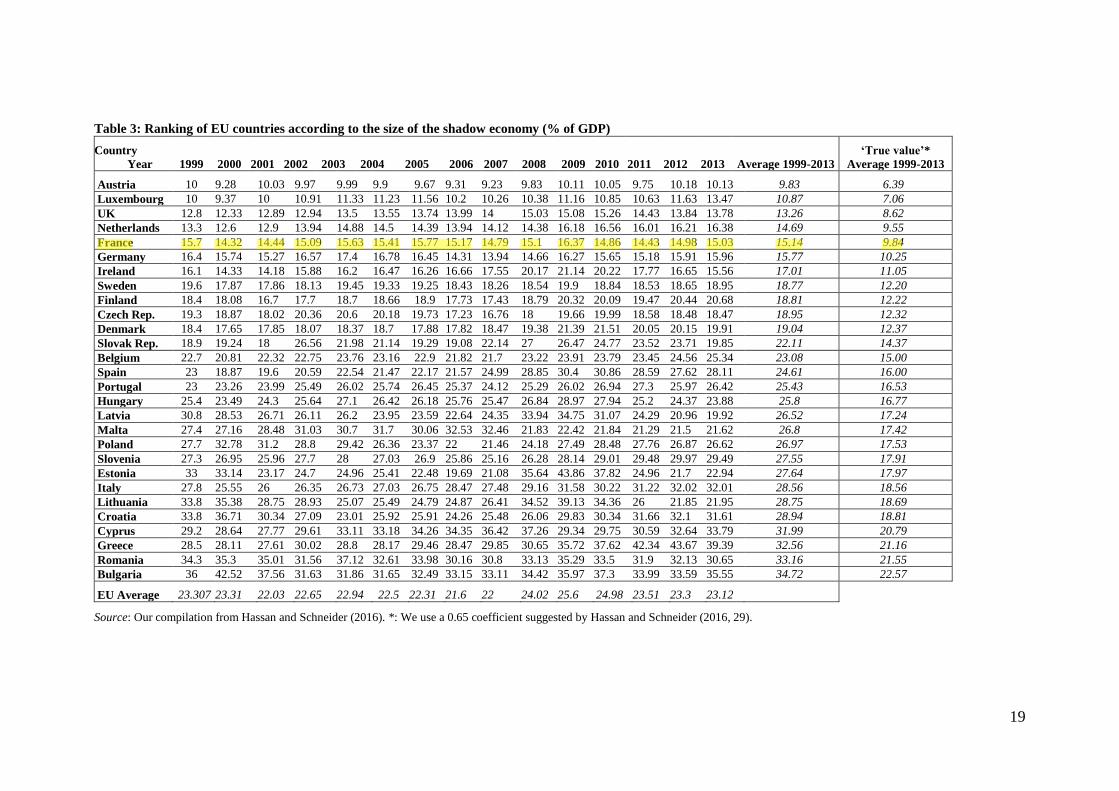
Table 3 allows to examine the magnitude of the SE relative to GDP according country ranking,
as well as the trends over a fifteen-year period (1999-2013).
Unemployment sheds little light on the SE and Enste (2010) provides unconvincing results in
this connection. Although poorer countries as regards GDP per capita, in Southern and Eastern
Europe, experience inefficient regulations and have the largest share of SE, it does not explain
why some richer countries (Denmark and Belgium) reach a fairly high size in NOE.
The size of SE grows moving from West to East and also from North to South, although without
displaying a clear pattern. Dividing the EU 28 into quartiles, the average size over the period
ranges from below 10% (Austria) up to 17% (Ireland) as for the first quartile, beyond 24%
(Spain) as for the second quartile, beyond to 27% (Estonia) as for the third quartile and beyond
33% (Bulgaria) as for the last quartile. Ranking remains stable overtime. 1
With respect to the EU average, the size of the SE fluctuates but declined throughout the 2000s,
although experiencing an upturn over 2008-2010 (See also Schneider, 2015). Actually,
monetary time series may fluctuate much more than non-monetary variables.
This declining trend may be explained thanks to improving regulations and enforcement
policies, as well as tax cuts (Schneider, 2009b).
Among non-monetary variables, tax morale is presumably asymmetrical: It may sharply
decrease albeit it will slowly increase.
Last but not least, the DYMIMIC/currency demand method provides estimates that seem
oversized for two main reasons. First, the scope of the SE is restricted to underground, informal
and household activities, regardless of illegal activities (N2), whereas currency demand applies
1 Trends from Schneider’s figures are consistent with those of Afonso and Almeida (2017) using the MIMIC
method and focusing upon the PIIGS (Portugal, Italy, Ireland, Greece and Spain) over 1980-2013. However,
including Ireland proves inconsistent over 1999-2013.
18
to all NOE categories; therefore calibration exceeds the scope. Second, so-called official GDP
is somehow adjusted as regards a fraction of NOE types, thus fully adjusted GDP (i.e. including
all NOE types) should generate a lower NOE/GDP ratio.
Hassan and Schneider. (2016) acknowledge that the MIMIC and/or currency demand approach
achieves high SE estimates. They claim that DIY (do-it-yourself) activities, help from
neighbours and friends (N3), as well as criminal activities (N2) are at least partly included.
Once deducted these activities roughly 65% of the SE remains, which should more accurately
reflect its “true” size.
We calculated the average true size of the SE (See last column in Table 3), using the 0.65
coefficient suggested by Hassan and Schneider (2016, 29). It does not affect the country
ranking, whereas it shrinks the absolute magnitude of SE estimates, which gets closer to albeit
above the NOE estimates, with few exceptions (e.g. Austria).
However, the magnitude and accuracy of this figure should be discussed. On the one hand,
stating that over one third (0.35) of the SE is made of the N3 + N2 categories does not fit the
data of EU countries for which the share of NOE components are available (See Table 1). On
the other hand, if those activities are included and they should be indeed according to the NOE
standard definition, why should they be dropped?
Using a Dynamic General Equilibrium (DGE) model, Elgin and Oztunali (2012) notice is that
the 1999-2007 part of their dataset is almost perfectly correlated with the SE data reported by
Schneider, supporting the hypothesis that the size of the SE is countercyclical. Elgin and
Schneider (2016) acknowledge that DGE and DYMIMIC models reach similar conclusions,
although the former smooths the fluctuations that are displayed in the latter.
19
Table 3: Ranking of EU countries according to the size of the shadow economy (% of GDP)
Country
Year 1999 2000 2001 2002 2003 2004 2005 2006 2007 2008 2009 2010 2011 2012 2013 Average 1999-2013
‘True value’*
Average 1999-2013
Austria 10 9.28 10.03 9.97 9.99 9.9 9.67 9.31 9.23 9.83 10.11 10.05 9.75 10.18 10.13 9.83 6.39
Luxembourg 10 9.37 10 10.91 11.33 11.23 11.56 10.2 10.26 10.38 11.16 10.85 10.63 11.63 13.47 10.87 7.06
UK 12.8 12.33 12.89 12.94 13.5 13.55 13.74 13.99 14 15.03 15.08 15.26 14.43 13.84 13.78 13.26 8.62
Netherlands 13.3 12.6 12.9 13.94 14.88 14.5 14.39 13.94 14.12 14.38 16.18 16.56 16.01 16.21 16.38 14.69 9.55
France 15.7 14.32 14.44 15.09 15.63 15.41 15.77 15.17 14.79 15.1 16.37 14.86 14.43 14.98 15.03 15.14 9.84
Germany 16.4 15.74 15.27 16.57 17.4 16.78 16.45 14.31 13.94 14.66 16.27 15.65 15.18 15.91 15.96 15.77 10.25
Ireland 16.1 14.33 14.18 15.88 16.2 16.47 16.26 16.66 17.55 20.17 21.14 20.22 17.77 16.65 15.56 17.01 11.05
Sweden 19.6 17.87 17.86 18.13 19.45 19.33 19.25 18.43 18.26 18.54 19.9 18.84 18.53 18.65 18.95 18.77 12.20
Finland 18.4 18.08 16.7 17.7 18.7 18.66 18.9 17.73 17.43 18.79 20.32 20.09 19.47 20.44 20.68 18.81 12.22
Czech Rep. 19.3 18.87 18.02 20.36 20.6 20.18 19.73 17.23 16.76 18 19.66 19.99 18.58 18.48 18.47 18.95 12.32
Denmark 18.4 17.65 17.85 18.07 18.37 18.7 17.88 17.82 18.47 19.38 21.39 21.51 20.05 20.15 19.91 19.04 12.37
Slovak Rep. 18.9 19.24 18 26.56 21.98 21.14 19.29 19.08 22.14 27 26.47 24.77 23.52 23.71 19.85 22.11 14.37
Belgium 22.7 20.81 22.32 22.75 23.76 23.16 22.9 21.82 21.7 23.22 23.91 23.79 23.45 24.56 25.34 23.08 15.00
Spain 23 18.87 19.6 20.59 22.54 21.47 22.17 21.57 24.99 28.85 30.4 30.86 28.59 27.62 28.11 24.61 16.00
Portugal 23 23.26 23.99 25.49 26.02 25.74 26.45 25.37 24.12 25.29 26.02 26.94 27.3 25.97 26.42 25.43 16.53
Hungary 25.4 23.49 24.3 25.64 27.1 26.42 26.18 25.76 25.47 26.84 28.97 27.94 25.2 24.37 23.88 25.8 16.77
Latvia 30.8 28.53 26.71 26.11 26.2 23.95 23.59 22.64 24.35 33.94 34.75 31.07 24.29 20.96 19.92 26.52 17.24
Malta 27.4 27.16 28.48 31.03 30.7 31.7 30.06 32.53 32.46 21.83 22.42 21.84 21.29 21.5 21.62 26.8 17.42
Poland 27.7 32.78 31.2 28.8 29.42 26.36 23.37 22 21.46 24.18 27.49 28.48 27.76 26.87 26.62 26.97 17.53
Slovenia 27.3 26.95 25.96 27.7 28 27.03 26.9 25.86 25.16 26.28 28.14 29.01 29.48 29.97 29.49 27.55 17.91
Estonia 33 33.14 23.17 24.7 24.96 25.41 22.48 19.69 21.08 35.64 43.86 37.82 24.96 21.7 22.94 27.64 17.97
Italy 27.8 25.55 26 26.35 26.73 27.03 26.75 28.47 27.48 29.16 31.58 30.22 31.22 32.02 32.01 28.56 18.56
Lithuania 33.8 35.38 28.75 28.93 25.07 25.49 24.79 24.87 26.41 34.52 39.13 34.36 26 21.85 21.95 28.75 18.69
Croatia 33.8 36.71 30.34 27.09 23.01 25.92 25.91 24.26 25.48 26.06 29.83 30.34 31.66 32.1 31.61 28.94 18.81
Cyprus 29.2 28.64 27.77 29.61 33.11 33.18 34.26 34.35 36.42 37.26 29.34 29.75 30.59 32.64 33.79 31.99 20.79
Greece 28.5 28.11 27.61 30.02 28.8 28.17 29.46 28.47 29.85 30.65 35.72 37.62 42.34 43.67 39.39 32.56 21.16
Romania 34.3 35.3 35.01 31.56 37.12 32.61 33.98 30.16 30.8 33.13 35.29 33.5 31.9 32.13 30.65 33.16 21.55
Bulgaria 36 42.52 37.56 31.63 31.86 31.65 32.49 33.15 33.11 34.42 35.97 37.3 33.99 33.59 35.55 34.72 22.57
EU Average 23.307 23.31 22.03 22.65 22.94 22.5 22.31 21.6 22 24.02 25.6 24.98 23.51 23.3 23.12
Source: Our compilation from Hassan and Schneider (2016). *: We use a 0.65 coefficient suggested by Hassan and Schneider (2016, 29).
20
5.2. Tax burden and NOE: some ambiguous links.
The robustness of the explanation that connects tax pressure with NOE is far from being proven.
The average (or marginal) tax rate of taxation may not matter as much as the tax structure with
respect to basis and thresholds; unfortunately, the latter varies across countries and among tax
payers (e.g. bachelor, families, etc) according to the average wages (OECD, 2006, 2009).
As regards levels, the correlation between NOE (as % of GDP) and tax burden (including Social
Security contributions, as % of GDP) is poor and improves but a little whenever logarithms are
computed. The upper bond of the countries with the highest share in NOE (above the EU
average) does not include those that have the largest percentage of tax burden in terms of GDP.
Correlation is poor for the group of so-called Southern countries (Greece, Italy, Spain and
Portugal) also including Belgium and Sweden, which obviously are not located in the same
area.
As the difference between the level of tax collected and the total tax owed, the tax gap can
broadly be split into two types of activities, tax evasion and tax avoidance. Raczkowski and
Mróz (2016) contend that the level of the tax gap is rather negatively correlated with GDP, i.e.
the higher the GDP is, the lower the tax gap as the percentage of the GDP. However, Italy is an
exception (See Table 4 in the appendix). The distribution of tax gaps does not match that of the
SE (Schneider, 2016), neither does the tax gap distribution of Muller et al (2013).
5.3. Labour market segmentation and informal workforce.
According to Packard et al (2012), the labour market is segmented between formal and informal
workforce. The latter consists in informal dependent employment and informal self-
employment (ILO, 2013). They observe significant differences in the composition and profile
of the informal workforce across the EU countries. In Bulgaria, Romania and Slovenia, the
informal workforce is roughly evenly split between dependent workers without a legal contract
and the nonprofessional self-employed. In contrast, informal self-employment is the dominant
form in the Czech Republic, Hungary, Lithuania, Poland and Slovakia. This split also applies
to Greece, Italy, Portugal and Spain. Unfortunately, Eurostat does not investigate informal
employment in the labour force survey.
Undeclared jobs seem to rise during recovery and to contract during recession, as for Spain and
Italy where informal employment is widespread and provides flexibility to various sectors. As
documented by Bajada and Schneider (2009), opportunities in the SE are fuelled by the
expansion of the official economy that is pro-cyclical and unemployment does not provide job
opportunities in the SE; thus there is no trade-off between economies because the income effect
21
offsets the substitution effect. This may also explain differences across European countries that
do not experience the same trends.
Correlation between NOE (as a % of GDP) and self-employment (as a % of non-agricultural
employment) is poor. The upper bond of the countries which have the highest share in NOE are
also those which have the largest percentage of non-agricultural self-employed population:
Correlation is high for Southern countries (Greece, Italy, Spain and Portugal). As regards the
lower bound of countries with the smallest share in NOE (Ireland, France, Netherlands, UK and
Austria), the percentage of non-agricultural self-employed population is far from being the
lowest and no correlation shows up. Although self-employed is the working group that complies
the less with tax requirements (underground economy) and represent a significant fraction of
unincorporated enterprises (informal economy), self-employed population is not a satisfactory
proxy for NOE.
6. Discussion and conclusion.
The DYMIMIC vs. National Accounts controversy looks like another hare-tortoise contest. In
contrast with the fable, DYMIMIC runs faster than National Accounts, but neither reach the
finishing line2. The former provides oversized estimates of the NOE, whereas the latter lags
behind due to the lack of exhaustiveness.
So far the DYMIMIC model was presented as exploratory and did not require a priori specified
factor. Recently, it has been claimed as explanatory (Elgin and Schneider, 2016), although there
is no explicit theory behind the model and econometric issues require robustness checks.
Macro-econometric models make strong assumptions, use highly aggregated data and have
little control over what exactly is being measured; it is unclear whether NOE includes adjusted
GDP or not. They provide times series that prove cheap to compute.
Similarly, there is no model in national accounts, it is the framework and procedures that shape
the estimates. Including standardised data on the illegal NOE type helps completing the scope
since 2014, although exhaustiveness is far from achievement. NOE estimates may be
conservative in as much as adjustments already include some components, although parameters
are not disclosed. Data are computed at a highly disaggregated level and double counting is
avoided, but timely regular estimates are lacking and should become available.
2 The absence of some available NOE estimates for informal labour provided by national accounts, and the use of
undeclared work figures from 2013 Eurobarometer that do not fit in the Eurostat nomenclature, alongside disparate
dates makes EC (2016, table 1, 3) a very misleading paper.
22
In the absence of consensus on the most reliable method (e.g. time-series data vs. cross-section
surveys), it seems that the search for an optimal indicator is still beyond reach. One may share
the claim from Ven (2017) advocating that both the national accounts and macro-econometric
models share the best in order to improve the scope and measurement of NOE, starting with the
disclosure of their data and procedures.
Moreover, the unemployment challenge is back on the agenda and calls upon both standardized
data and closer monitoring of undeclared work (EC, 2016), provided that data resist political
interference (Tanzi 1999) or misuses (Dixon 1999).
References
Adair, P. 2009. Economie non observée et emploi informel dans les pays de l’Union européenne
– Une comparaison des estimations et des déterminants, Revue Economique, 60(5): 1117-
1153.
Adair, P., Nezhyvenko, O. 2016. Sex work vs. sexual exploitation in the European Union: What
are the likely guesstimates for prostitution?" Proceedings 6th Economics & Finance
Conference, OECD, Paris, September 6-9. IISES, pp. 27-50 DOI:
10.20472/EFC.2016.006.002
Afonso, O., Almeida, F. 2017. The non-observed economy in the European Union, Applied
Economics Letters, 24(1): 14-18
Ahumada, H., Alvaredo, F., Canavese, A. 2008. The monetary method to measure the shadow
economy: The forgotten problem of the initial conditions, Economics Letters, 101: 97–99.
Barthélémy, P. 1988. The macroeconomic estimates of the hidden economy: a critical analysis,
Review of Income and Wealth, 34(2): 183-208.
Bajada, C. and Schneider, F. 2009. Unemployment and the Shadow Economy in the OECD,
Revue Economique 60(5): 1033–1067.
Barthélémy, P., Miguelez, F., Mingione, E., Pahl, R. and Wenig, A. 1990. Underground
Economy and Irregular Forms of Employment (travail au noir). Commission of the
European Communities, Brussels.
Bhattacharyya, D. K. 1999. On the Economic Rationale of Estimating the Hidden Economy,
The Economic Journal 109: 348-359.
Blades, D. 2011. Estimating value added of illegal production in the Western Balkans. Review
of Income & Wealth, 57(1): 183-195.
Blades, D., Roberts, D. 2002. Measuring the Non Observed Economy, Statistics Brief 5,
November, OECD.
23
Breusch, T. 2005. Estimating the Underground Economy using MIMIC Models, The Australian
National University, November, Canberra.
Cagan, P. 1958. The demand for currency relative to the total money supply, Journal of
Political Economy 66: 303-328.
Contini, B. 1989. The irregular economy of Italy: a survey of contributions. In: Feige, E.L.
(Ed.), pp. 237-250.
Dilnot, A., Morris, C.N. 1981. What do we know about the black economy? Fiscal Studies 2(1):
58-73.
Dixon, H. 1999. Controversy: on the use of the ‘hidden economy’ estimates, Economic Journal
109: 335-337.
Dybka, P., Kowalczuk ,M., Olesinski, B., Rozkrut, M., Torój, A. 2017. Currency demand and
MIMIC models: towards a structured hybrid model-based estimation of the shadow economy
size. Warsaw School of Economics, Working Papers Series N° 2017/030, September
EC. 2004. European Employment Observatory Review, Autumn, European Commission
Directorate-General for Employment, Social Affairs and Equal Opportunities, Brussels.
EC. 2006. Non Observed Economy in National Accounts, Economic and Social Council, Expert
Group on National Accounts, Economic Commission for Europe, Brussels.
EC 2007. European Employment Observatory Review, Spring, European Commission
Directorate-General for Employment, Social Affairs and Equal Opportunities, Brussels.
EC. 2016. European Semester Thematic Factsheet- Undeclared Work. European Commission,
November. https://ec.europa.eu/.../european-semester_thematic-factsheet_undeclared work
EEC. 2013. Undeclared Work in the European Union, European Commission, Directorate
General Employment & Social Affairs, Special Euro barometer 402, Brussels.
EEC. 2007. Undeclared Work in the European Union, European Commission, Directorate
General Employment & Social Affairs, Special Euro barometer 284, Brussels.
Elgin, C., Oztunali, O. 2012. Shadow economies around the world: model based estimates.
Working Paper 2012/05, Boğaziçi University, Department of Economics.
Elgin C. and Schneider F. 2016. Shadow Economies in OECD Countries: DGE vs. MIMIC
Approaches. Boğaziçi Journal Review of Social, Economic and Administrative Studies,
30(1): 51-75.
Ernste D. 2010. Shadow Economy – The Impact of Regulation in OECD-countries.
International Economic Journal 24(4): 555-571
Eurostat. 2014. Essential SNA: Building the basics, chapter 6: The Informal Sector, pp. 121-
134, Methodologies and working papers, European Union, Luxemburg
24
Feige, E. L. 2016. Reflections on the Meaning and Measurement of Unobserved Economies:
What do we really know about the “Shadow Economy”? Journal of Tax Administration 2(1):
5-41
Frey, B. S., Weck-Hannemann, H. 1984. The hidden economy as an ‘unobserved variable,
European Economic Review 26: 33-53.
Gutmann, P. 1985. “The subterranean economy, redux”. In Gaertner, W. and Wenig, A. Eds.
The Economics of the Shadow Economy, Springer Verlag, Berlin, pp. 2-18
Giles, D. E. A. 1999. Measuring the Hidden Economy: Implications for Econometric
Modelling, The Economic Journal, 109: 370-380.
Gyomai, G., Ven van de, P. 2014. The Non Observed Economy in the System of National
Accounts, OECD Brief, 18, June.
Hassan, M., Schneider, F. 2016. Size and Development of the Shadow Economies of 157
Countries Worldwide: Updated and New Measures from 1999 to 2013. IZA DP No. 10281
October
Helberger, C., Knepel, H. 1988. How big is the shadow economy? A re-analysis of the
unobserved-variable approach of Frey and Weck-Hannemann, European Economic Review
32: 965-976.
Kaufmann, D., Kaliberda, A.1996. Integrating he unofficial into the dynamics of post-socialist
economies, in: Kaminsky, B. Ed. Economic Transition in the Newly Independent States, M.
E. Sharpe, pp. 81-120.
Kayaoglu, A., Williams, C. C. 2017. Beyond the declared/undeclared economy dualism:
evaluating individual- and country-level variations in the prevalence of under-declared
employment. International Journal of Economic Perspectives. Forthcoming.
Lackó, M. 2000. Do Power Consumption Data Tell the Story? Electricity Intensity and Hidden
Economy in Postsocialist Countries, in Maskin, E. and Simonovits, A. Eds. Planning,
Shortage, and Transformation. MIT Press, Cambridge (Mass.) and London, pp. 345-366.
Medina L., Schneider, F. 2017. Shadow Economies around the World: New Results for 158
Countries over 1991-2015. Johannes Kepler Linz University working paper 1710, July.
Lippert, O., Walker, M. Eds. 1997. The Underground Economy: Global Evidence of its Size
and Impact, Frazer Institute, Vancouver.
Lyssiotou, P., Pashardes, P., Stengos, T. 2004. Estimates of the black economy based on
consumer demand approaches, Economic Journal 114:.622-640.
25
Muller, P., Conlon, G., Lewis, M., Mantovani, I. 2013. From Shadow to Formal Economy:
Levelling the Playing Field in the Single Market. European Parliament
http://www.europarl.europa.eu/studies
OECD. 2002. Handbook for Measurement of the Non-Observed Economy, OECD, Paris.
OECD. 2004. Employment Outlook, chapter 5, “Informal Employment and Promoting the
Transition to a Salaried Economy”, pp. 225-289, OECD, Paris.
OECD. 2006. Employment Outlook, table 2 - Evolution of the tax burden 2000-2005,
www.oecd.org/dataoecd/50/39/36371872.pdf
OECD. 2009. Employment Outlook, OECD, Paris.
Packard T., Koettl J., Montenegro C.E. 2012. In From the Shadow – Integrating Europe’s
Informal Labor. The World Bank
Pissarides, C., Weber, G. 1989. An expenditure-based estimate of Britain’s black economy,
Journal of Public Economics 39(1):.17-32.
Raczkowski, K., Mróz B. 2016. Tax gap in the global economy, Argumenta Oeconomica
Working paper, Wroclaw University of Economics.
Schneider F. 2015. Size and development of the shadow economy of 31 European countries
and 5 other OECD countries from 2003 to 2015: Different Developments.
http://www.econ.jku.at/membrs/Schenider/filers/publications/2015/ShadEcEurope31.pdf.
[31.3.2016]
Schneider, F. 2009a. The Size of the Shadow Economy in 21 OECD Countries (in % of
‘official’ GDP) using the MIMIC and currency demand approach: From 1989/90 to 2009,
Working Paper, April, University of Linz.
Schneider, F. 2009b. Size and Development of the Shadow Economies in Germany, Austria
and other OECD Countries, Revue Economique 60(5): 1079-1116.
Schneider, F. and Enste, D. H. 2000. Shadow Economies: Size, Causes and Consequences,
Journal of Economic Literature, 38: 77-114.
Schneider, F., Raczkowski, K., Mróz, B. 2015. Shadow economy and tax evasion in the EU,
Journal of Money Laundering Control 18(1): 34-51
Schneider, F. and Williams, C. C. 2013. The Shadow Economy. The Institute of Economic
Affairs- IEA, London.
Tanzi, V. Ed. 1982. The Underground Economy in the US and Abroad, Lexington Books
Tanzi, V. 1999. Uses and Abuses of Estimates of the Underground Economy’, Economic
Journal 109: 338-347.
26
Thomas, J. J. 1992. Informal Economic Activity, LSE Handbooks in Economics, Harvester
Wheatsheaf.
Thomas, J. J. 1999. Quantifying the Black Economy: ‘Measurement without Theory’ yet again?
Economic Journal, 109: 381-389.
UNECE. 2003. Non-Observed Economy in National Accounts – Survey of National Practices,
United Nations Economic Commission for Europe, Geneva.
UNECE. 2008. Non-Observed Economy in National Accounts – Survey of National Practices,
United Nations Economic Commission for Europe, Geneva.
World Bank. 2007. Concept of informal sector, http:/Inweb18.
worldbank.org/eca/eca.nsf/Sectors.
Ven van de P. 2017. The Non-Observed Economy in the System of National Accounts. Illicit
Financial Flows and Underground Economy in Developing and Developed Countries: A
Mirror Conference, Leuven, 22-23 May.
27
Appendix
Table 4. Illegal production (N2) in the EU countries
Country Year
*
% of
GDP Year
** % of
GDP
Year
*** % of
GDP Country
Year
*
% of
GDP Year
** % of
GDP
Year
*** % of
GDP
Austria 2008 0.2 2010 0.16 Italy 2010 1
Belgium 2010 0.37 Latvia 1998 0.97 2000 1.5 2010
Bulgaria 1999 1.3 2010 0.21, Lithuania 1998 0.5 2002 0.9 2010 0.9
Croatia 2003 0.52 2006 0.86 2010 0.7 Luxembourg 2010 0.23
Cyprus 2010 1.09 Malta 2010 0.3
Czech Rep. 2010 0.53 Netherlands 2007 0.5 2010 0.38
Denmark 2010 0.14 Poland 1998 0.13 2009 0.9 2010
Estonia 1998 0.8 2006 0.6 2010 0.52 Portugal 2010 0.35
Finland 2010 0.1 Romania 2010 0.46
France 2010 Slovak Rep. 1998 0.59 2009 0.5 2010
Germany 2010 0.1 Slovenia 2007 0.3 2010 0,36
Greece 2010 Spain 2010 0.87
Hungary 2010 0.85 Sweden 2010 0,14
Ireland 2010 0.73 UK 2010 0.58 Source: * UNECE (2003); ** Blades (2011); *** Adair and Nezhyvenko (2016)
Table 5. Tax gaps in the EU (% of GDP)
Member State 2011 Member State 2011 Member State 2015 Member State 2015
Luxembourg 1.2 Portugal 2.4 Luxembourg 1.7 Portugal 7.5
Austria 1.3 Sweden 2.6 Ireland 2.9 EU 28 7.7
UK 1.4 Denmark 2.7 Denmark 3.1 France 8.2
Ireland 1.5 Lithuania 2.7 UK 3.2 Latvia 8.3
Greece 1.6 Romania 2.7 Netherlands 3.5 Bulgaria 8.3
Netherlands 1.7 Poland 2.8 Austria 4.3 Poland 9
Slovak Rep. 1.7 Malta 2.9 Finland 5 Belgium 9.4
Czech Rep. 2 Belgium 3 Croatia 5.2 Malta 10.1
Germany 2 Cyprus 3.1 Cyprus 5.8 Hungary 10.5
France 2 Bulgaria 3.2 Germany 6 Spain 10.6
Spain 2.3 Hungary 3.2 Sweden 6.5 Lithuania 11
Latvia 2.3 Slovenia 3.3 Slovak Rep. 6.9 Greece 11.2
EU 27 2.3 Estonia 3.5 Czech Rep. 7.3 Romania 12.1
Finland 2.4 Italy 3.8 Slovenia 7.5 Estonia 12.9
Portugal 7.5 Italy 13.5
Source: Muller et al (2013), Raczkowski and Mróz (2016)