Embed Size (px)
Citation preview
Wis
cons
in H
ighw
ay R
esea
rch
Prog
ram
Non-Nuclear Density Testing Devices and Systems to
Evaluate In-Place Asphalt Pavement Density
SPR# 0092-05-10
Robert Schmitt University of Wisconsin-Platteville
Chetana Rao and Harold Von Quintus Applied Research Associates, Inc.
May 2006
WHRP 06-12
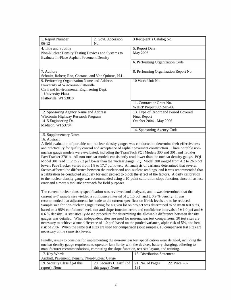
1. Report Number 06-12
2. Govt. Accession No.
3 Recipient’s Catalog No.
4. Title and Subtitle Non-Nuclear Density Testing Devices and Systems to Evaluate In-Place Asphalt Pavement Density
5. Report Date May 2006
6. Performing Organization Code
7. Authors Schmitt, Robert; Rao, Chetana; and Von Quintus, H.L.
8. Performing Organization Report No.
9. Performing Organization Name and Address University of Wisconsin-Platteville Civil and Environmental Engineering Dept. 1 University Plaza Platteville, WI 53818
10 Work Unit No.
11. Contract or Grant No. WHRP Project 0092-05-06
12. Sponsoring Agency Name and Address Wisconsin Highway Research Program 1415 Engineering Dr. Madison, WI 53704
13. Type of Report and Period Covered Final Report October 2004 - May 2006
14. Sponsoring Agency Code 15. Supplementary Notes 16. Abstract A field evaluation of portable non-nuclear density gauges was conducted to determine their effectiveness and practicality for quality control and acceptance of asphalt pavement construction. Three portable nonnuclear gauge models were evaluated, including the TransTech PQI Models 300 and 301, and Troxler PaveTracker 2701b. All non-nuclear models consistently read lower than the nuclear density gauge. PQI Model 301 read 11.2 to 27.2 pcf lower than the nuclear gauge; PQI Model 300 ranged from 4.2 to 26.6 pcf lower; PaveTracker varied from 1.8 to 17.7 pcf lower. An analysis of variance determined that several factors affected the difference between the nuclear and non-nuclear readings, and it was recommended that a calibration be conducted uniquely for each project to block the effect of the factors. A daily calibration to the nuclear density gauge was recommended using a 10-point calibration slope function, since it has less error and a more simplistic approach for field purposes.
The current nuclear density specification was reviewed and analyzed, and it was determined that the current n=7 sample size yielded a confidence interval of ± 1.5 pcf, and ± 0.9 % density. It was recommended that adjustments be made to the current specification if risk levels are to be reduced. Sample size for non-nuclear gauge testing for a given lot on project was determined to be n=30 test sites, based on a 95% confidence level, mat and slope-function error, and confidence intervals of ± 1.0 pcf and ± 0.6 % density. A statistically-based procedure for determining the allowable difference between density gauges was detailed. When independent sites are used for non-nuclear test comparisons, 30 test sites are necessary to achieve a true difference of 1.0 pcf, based on the pooled variance, alpha risk of 5%, and beta risk of 20%. When the same test sites are used for comparison (split sample), 10 comparison test sites are necessary at the same risk levels.
Finally, issues to consider for implementing the non-nuclear test specification were detailed, including the nuclear density gauge requirement, operator familiarity with the devices, battery charging, adhering to manufacturer recommendations, computing the slope function, test site layout, and training. 17. Key Words Asphalt, Pavement, Density, Non-Nuclear Gauge
18. Distribution Statement
19. Security Classif.(of this report) None
20. Security Classif. (of this page) None
21. No. of Pages 131
22. Price -0
2

DISCLAIMER
This research was funded through the Wisconsin Highway Research Program by the Wisconsin Department of Transportation (WisDOT) under Project # 0092-05-10. The contents of this report reflect the views of the authors who are responsible for the facts and the accuracy of the data presented herein. The contents do not necessarily reflect the official views of the WisDOT at the time of publication.
3
EXECUTIVE SUMMARY
This report conducted a field evaluation of portable non-nuclear density gauges to determine their effectiveness and practicality for quality control and acceptance of asphalt pavement construction. It was determined that non-nuclear density gauges can be used to measure in-place asphalt pavement density if they are calibrated to nuclear density gauges and a specified number of sample test sites are used.
A literature review of previous field studies generally found a comparison of cores with the non-nuclear Pavement Quality Indicator (PQI) gauge, non-nuclear PaveTracker gauge, and/or a nuclear density gauge. The studies found a bias between cores and both the nuclear and non-nuclear gauges on all projects. Bias, or the difference between the non-nuclear gauge and either the core or nuclear gauge, was generally below 10 pcf. When recommendations were stated in a study, non-nuclear devices could be used for quality control, however, they were not recommended for quality assurance or acceptance testing. Bias correction factors were also recommended using a single additive value.
Three portable non-nuclear gauge models were evaluated in this study, including the TransTech PQI 300, TransTech PQI 301, and Troxler PaveTracker 2701b. A CPN MC-3 nuclear density gauge was compared to the non-nuclear gauges; six-inch diameter cores were tested to ensure nuclear gauge calibration. A total of 16 individual HMA projects were used to compare the gauges and cores. Ten of the 16 projects included testing on multiple days and/or multiple mixture types.
A consistent finding was a bias between nuclear and non-nuclear gauges, and a change in bias within a project between days or a different mixture type. All non-nuclear models consistently read lower than the nuclear gauge. PQI Model 301 read 11.2 to 27.2 pcf lower than the nuclear gauge, while PQI Model 300 ranged from 4.2 to 26.6 pcf lower. PaveTracker varied from 1.8 to 17.7 pcf lower.
An analysis of variance determined that several factors affected the difference between the nuclear and non-nuclear readings, including aggregate source, design ESALs, passing no. 4 sieve, lab air voids, asphalt content, aggregate specific gravity, and pavement layer thickness. The analysis also confirmed that moisture values for PQI models must be below a value of 10, as stated in manufacturer recommendations, to yield valid test results.
Since many of the factors affecting non-nuclear density readings are mixture or project specific, it was recommended that a calibration be conducted uniquely for each project to offset or block the effect of the factors. Calibration to only the nuclear density gauge was recommended. Several other calibration types were investigated but they were not suitable at this time, including operating the gauges directly after warm up, WisDOT test blocks, manufacturer reference block, and Superpave gyratory specimens.
Three calibration functions were investigated using sets of 3, 5, and 10 random points, including: (1) intercept by adding a constant correction factor, (2) slope by multiplying a constant correction factor, and (3) slope-intercept by multiplying a slope term and adding
4
an intercept term. It was recommended that a 10-point calibration using the slope function be used over the slope-intercept function, since it has less error and a more simplistic approach for field purposes. The intercept function, commonly recommended in other studies, had substantially more error with the PQI 300 and was not recommended.
The stability of the 10-point slope function computed from Day 1 paving was applied to Day 2 raw non-nuclear readings to assess the feasibility on a typical multi-day paving project. The results indicated that a Day 2 slope function used to adjust Day 2 readings was more accurate than a Day 1 slope function used to adjust Day 2 readings. PaveTracker produced less error than both PQI models when the Day 1 slope function was applied to Day 2 raw non-nuclear readings.
The current nuclear density specification was reviewed and analyzed, and it was determined that the current n=7 sample size, coupled with a 95% probability level (5% risk) and mat standard deviation of 2.0 pcf, yielded a confidence interval of ± 1.5 pcf, and ± 0.9 % density. This indicated that both WisDOT and contractors are exposing themselves to greater risk than the recommended 5% level. Based on a sample size of n=7 and mat standard deviation of 2.0 pcf, the probability level of the finding the average density within ± 1.0 pcf was estimated to be 81.4%. The probability level of the finding the average within ± 0.5 % density was 70.4%. It was recommended that adjustments be made to the current nuclear density specification if risk levels are to be reduced from current levels.
Sample size for non-nuclear gauge testing for a given lot on a project was determined to be n=30 test sites, based on a 95% confidence level, both mat and slope-function error, and confidence intervals of ± 1.0 pcf and ± 0.6 % density. To reduce the confidence interval to ± 0.5 % density, a total of n=50 samples would be necessary.
A statistically-based procedure for determining the allowable difference between density gauges was detailed. The current QA test verification procedure, that compares two nuclear density gauges on QMP projects, was investigated. It was determined that when independent sites are used for non-nuclear testing, 30 test site comparisons are necessary to achieve a true difference of 1.0 pcf, based on the stated risk levels and pooled variance. When the same test sites are used for comparison (split sample), 10 comparison test sites are necessary to achieve a true difference of 1.0 pcf, at an alpha risk of 5%, and beta risk of 20%. The power concept was illustrated to determine the true mean difference between gauges by compensating for alpha and beta risks.
Finally, issues to consider for implementing the non-nuclear test specification were detailed. Several aspects require consideration including, the nuclear density gauge requirement to calibrate non-nuclear density gauges, operator familiarity with the nonnuclear gauges, battery charging, adhering to manufacturer recommendations, computing the slope function, test site layout, and training.
5

ACKNOWLEDGMENTS
The authors thank Wisconsin DOT and contractors for their valuable cooperation during this research study. The authors also thank UW-Platteville engineering students, Mr. Aaron Christ and Mr. Nicholas Hoernke, along with ARA engineers, Mr. Steve Ashe, Mr. Brandon Artis, Mr. Lewis Lingefelter, Ms. Kim Clark, Mr. Joseph Stefanski, and Jag Malella. A special thanks goes to the following Wisconsin DOT, contractor, and consultant personnel for their time and assistance during the field study.
Wisconsin DOT Steve Ames – D5 Mathy Construction Eric Arneson – D4 Erv Dukatz Cindy Belcher - Central Materials Tim Jones Wayne Chase – D1 Dave Lange Chris Chudy – D2 Don Ostreng Robert Cullins – D7 Prentiss Smith Ricky Davies – D2 Judie Tronson Pam Deneys – D3 Jason Weiker Bob Lemcke – D1 Lorie Peterson – D5 Northeast Asphalt, Inc. Judie Ryan – Central Materials Howard Anthony Ed Sanchez – D1 Chad Ebert Robert Schiro - Central Materials Mark Gasior Terry Sossaman – D2 Jay Rosemeyer Robin Stafford – D7 Karl Runstrom Oscar Winger – D5 Jason Skarda
Craig VanBeek B.R. Amons and Sons Paula Young Tom Amons Rod Anthony Payne and Dolan, Inc. Mike Biersack Mike Benish Adam Blanchard Efferin Dixon Mark Geherke Mark Genrich Joe Kyle Ryan Jennara Ron Staples Adam Lyters
Michelle McCorille D.L. Gasser Construction Lisa McNaught Pat Anderson Signe Reichelt Stephanie Brandt Dan Sutkowski Mike Byrnes John Troxler Rock Roads, Inc.
Steve Bloedow Jeff Wood
6

Stark Asphalt S.E.H. Chuck Gassert Dan Schultz Shannon Knoll Bill Kotz TN & Associates Don Stark Chad Bigler Gerry Waelti
R.E.I. American Asphalt Keith Klubenow Tom Burch Tom Marshke Bernie Grawski Regina Hoffman Gremmer and Assoc. Dave Jones Lane Wetterau John Montgomery Steve Smith Aguinaga Testing Services Jeff Weisman Rich Aguinaga
Mead and Hunt, Inc. Troxler Chris Neis Pat Schroeder Tim Verhege
Transtech Systems Quest Jaret Morse Blake Elsinger
7
TABLE OF CONTENTS
EXECUTIVE SUMMARY ................................................................................................ 4 ACKNOWLEDGMENTS .................................................................................................. 6 LIST OF FIGURES .......................................................................................................... 10 LIST OF TABLES............................................................................................................ 12 CHAPTER 1 INTRODUCTION ..................................................................................... 15
1.1 Background and Problem Statement ...................................................................... 15 1.2 Objective................................................................................................................. 15 1.3 Background and Significance of Work .................................................................. 15 1.4 Benefits ................................................................................................................... 16
CHAPTER 2 LITERATURE REVIEW .......................................................................... 17 2.1 Introduction ............................................................................................................ 17 2.2 Non-Nuclear Compactor-Mounted Systems .......................................................... 17 2.3 Non-Nuclear Portable Devices ............................................................................... 18 2.4 Previous Studies ..................................................................................................... 19
CHAPTER 3 EXPERIMENTAL DESIGN..................................................................... 23 3.1 Introduction ............................................................................................................ 23 3.2 Work Plan Parameters ............................................................................................ 23
CHAPTER 4 DATA COLLECTION SUMMARY ........................................................ 26 4.1 Projects ................................................................................................................... 26 4.2 Comparison of Cores and Research Nuclear Density Gauge ................................. 26 4.3 Comparison of Nuclear Density Gauges ................................................................ 28 4.4 Comparison of Nuclear and Non-Nuclear Density Gauges.................................... 30 4.5 Test Blocks ............................................................................................................. 32 4.6 PaveTracker Comparison between SGC Specimens and Mat................................ 33
CHAPTER 5 ANALYSIS OF FACTORS ...................................................................... 36 5.1 Introduction ............................................................................................................ 36 5.2 Analysis of Variance .............................................................................................. 36 5.3 Results of ANOVA for All Project Gauges............................................................ 37 5.4 Results of ANOVA for Difference between Nuclear and Non-Nuclear Gauges ... 43 5.5 Summary of Factors Analysis................................................................................. 53
CHAPTER 6 INVESTIGATION OF CALIBRATION PROCEDURES ....................... 54 6.1 Introduction ............................................................................................................ 54 6.2 Calibration Procedures ........................................................................................... 54 6.3 Development of Calibration Procedures................................................................. 55 6.4 Approach to Calculate Adjustment Factor ............................................................. 62 6.5 Intercept Function................................................................................................... 64 6.6 Slope Function........................................................................................................ 72 6.7 Slope and Intercept Function.................................................................................. 79 6.8 Calculation of Mean Squared Errors for All Mix IDs ............................................ 85 6.9 Statistical Verification of Calibration Functions .................................................... 97 6.10 Stability of 10-Point Slope Function on Multiple Days Paving ......................... 102 6.11 Investigation of Moisture Correction for PQI Models ....................................... 104
8
CHAPTER 7 NON-NUCLEAR QC/QA ANALYSIS .................................................. 107 7.1 Introduction .......................................................................................................... 107 7.2 Current WisDOT Specification ............................................................................ 107 7.3 Sample Size Determination for Non-Nuclear Gauges.......................................... 112 7.4 Tolerance between Two Non-Nuclear Devices.................................................... 114
CHAPTER 8 IMPLEMENTATION.............................................................................. 123 8.1 Introduction .......................................................................................................... 123 8.2 Implementation Issues .......................................................................................... 123
CHAPTER 9 CONCLUSIONS AND RECOMMENDATIONS.................................. 125 9.1 Conclusions .......................................................................................................... 125 9.2 Recommendations ................................................................................................ 127
REFERENCES ............................................................................................................... 128 APPENDIX A................................................................................................................. 130
9
LIST OF FIGURES
FIGURE 5.1 EFFECT OF PASSING NO. 4 SIEVE ON DENSITY READINGS......... 39 FIGURE 5.2 EFFECT OF LAB AIR VOIDS ON DENSITY READINGS ................... 39 FIGURE 5.3 RELATIONSHIP OF AGGREGATE BSG ON DENSITY READINGS. 40 FIGURE 5.4 RELATIONSHIP OF AGGREGATE SOURCE ON DENSITY
READINGS................................................................................................................ 41 FIGURE 5.5 RELATIONSHIP OF FINE-GRADED AGGREGATE SOURCES ON
FIGURE 5.6 GMM PROJECT VALUES BASED ON AGGREGATE SOURCE TYPE DENSITY READINGS.............................................................................................. 41
.................................................................................................................................... 42 FIGURE 5.7 PQI 300 TEMPERATURE-DENSITY RELATIONSHIP ........................ 42 FIGURE 5.8 PQI 301 TEMPERATURE-DENSITY RELATIONSHIP ........................ 43 FIGURE 5.9 RELATIONSHIP OF NMAS AND DIFFERENCE OF DENSITY
READINGS................................................................................................................ 45 FIGURE 5.10 RELATIONSHIP OF SOURCE AND DIFFERENCE OF DENSITY
FIGURE 5.11 RELATIONSHIP OF DESIGN ESALS AND DIFFERENCE OF
FIGURE 5.12 RELATIONSHIP OF PASSING NO.4 SIEVE AND DIFFERENCE OF
FIGURE 5.13 RELATIONSHIP OF LAB AIR VOIDS AND DIFFERENCE OF
FIGURE 5.14 RELATIONSHIP OF ASPHALT CONTENT AND DIFFERENCE OF
FIGURE 5.15 RELATIONSHIP OF AGGREGATE BULK SPECIFIC GRAVITY AND
FIGURE 5.16 RELATIONSHIP OF PAVEMENT THICKNESS AND DIFFERENCE
FIGURE 5.17 PQI 300 RELATIONSHIP OF TEMPERATURE AND DIFFERENCE
FIGURE 5.18 PQI 301 RELATIONSHIP OF TEMPERATURE AND DIFFERENCE
FIGURE 5.19 PQI 300 RELATIONSHIP OF MOISTURE AND DIFFERENCE OF
FIGURE 5.20 PQI 301 RELATIONSHIP OF MOISTURE AND DIFFERENCE OF
FIGURE 6.1 STANDARD DEVIATION COMPARISON OF NUCLEAR READINGS
FIGURE 6.2 FREQUENCY OF STANDARD DEVIATION IN CLUSTERED
FIGURE 6.3 FREQUENCY OF STANDARD DEVIATION IN CLUSTERED
READINGS................................................................................................................ 46
DENSITY READINGS.............................................................................................. 46
DENSITY READINGS.............................................................................................. 47
DENSITY READINGS.............................................................................................. 48
DENSITY READINGS.............................................................................................. 48
DIFFERENCE OF DENSITY READINGS .............................................................. 49
OF DENSITY READINGS ....................................................................................... 50
OF MC3 DENSITY READINGS .............................................................................. 51
OF MC3 DENSITY READINGS .............................................................................. 51
MC3 DENSITY READINGS .................................................................................... 52
MC3 DENSITY READINGS .................................................................................... 52
AND NON-NUCLEAR CLUSTER .......................................................................... 59
TESTING FOR MIX #1............................................................................................. 60
TESTING FOR MIX #17........................................................................................... 60 FIGURE 6.4 DENSITY MEASUREMENT COMPARISON FOR MIX #1.................. 61 FIGURE 6.5 DENSITY MEASUREMENT COMPARISON FOR MIX #17................ 61
10
FIGURE 6.6 CORRECTED VS. ACTUAL DENSITY READINGS USING INTERCEPT FUNCTION AND 3 RANDOM POINTS (MIX ID #17) ................... 71
FIGURE 6.7 CORRECTED VS. ACTUAL DENSITY READINGS USING
FIGURE 6.8 CORRECTED VS. ACTUAL DENSITY READINGS USING
FIGURE 6.9 CORRECTED VS. ACTUAL DENSITY READINGS USING SLOPE
FIGURE 6.10 CORRECTED VS. ACTUAL DENSITY READINGS USING SLOPE
FIGURE 6.11 CORRECTED VS. ACTUAL DENSITY READINGS USING SLOPE
FIGURE 6.12 CORRECTED VS. ACTUAL DENSITY READINGS USING SLOPE
FIGURE 6.13 CORRECTED VS. ACTUAL DENSITY READINGS USING SLOPE
FIGURE 6.14 CORRECTED VS. ACTUAL DENSITY READINGS USING SLOPE
FIGURE 6.15 MEAN SQUARED ERROR FOR CALIBRATION FUNCTIONS
FIGURE 6.16 MEAN SQUARED ERROR FOR CALIBRATION FUNCTIONS
FIGURE 6.17 MEAN SQUARED ERROR FOR CALIBRATION FUNCTIONS
INTERCEPT FUNCTION AND 5 RANDOM POINTS (MIX ID #17) ................... 71
INTERCEPT FUNCTION AND 10 RANDOM POINTS (MIX ID #17) ................. 72
FUNCTION AND 3 RANDOM POINTS (MIX ID #17) ......................................... 77
FUNCTION AND 5 RANDOM POINTS (MIX ID #17) ......................................... 78
FUNCTION AND 10 RANDOM POINTS (MIX ID #17) ....................................... 78
INTERCEPT FUNCTION AND 3 RANDOM POINTS (MIX ID #17) ................... 83
INTERCEPT FUNCTION AND 5 RANDOM POINTS (MIX ID #17) ................... 84
INTERCEPT FUNCTION AND 10 RANDOM POINTS (MIX ID #17) ................. 84
USING 3 RANDOM POINTS................................................................................... 95
USING 5 RANDOM POINTS................................................................................... 96
USING 10 RANDOM POINTS................................................................................. 96 FIGURE 6.18 MOISTURE CORRECTION FOR PQI 300 USING POOLED DATA 104 FIGURE 6.19 MOISTURE CORRECTION FOR PQI 301 USING POOLED DATA 105 FIGURE 6.20 MOISTURE CORRECTION FOR PQI 300 FROM MIX ID #17 ....... 106 FIGURE 6.21 MOISTURE CORRECTION FOR PQI 300 FROM MIX ID #17 ....... 106 FIGURE 7.1 ILLUSTRATION OF POWER CONCEPT FOR DETECTING A TRUE
MEAN DIFFERENCE............................................................................................. 119
11
LIST OF TABLES
TABLE 2.1 COMPACTOR-MOUNTED NON-NUCLEAR DEVICE MANUFACTURERS ................................................................................................ 18
TABLE 2.2 PORTABLE NON-NUCLEAR DEVICE MANUFACTURERS ............... 19 TABLE 2.3 SUMMARY OF FIELD RESEARCH STUDIES EVALUATING NON
NUCLEAR DEVICES ............................................................................................... 20 TABLE 4.1 PROJECT ATTRIBUTES ........................................................................... 26 TABLE 4.2 CORE AND NUCLEAR GAUGE COMPARISON ................................... 27 TABLE 4.3 NUCLEAR DENSITY GAUGE COMPARISON ...................................... 29 TABLE 4.4 NUCLEAR AND NON-NUCLEAR GAUGE COMPARISON................. 31 TABLE 4.5 TRUAX LAB TEST BLOCK RESULTS ................................................... 32 TABLE 4.6 DISTRICT 4 TEST BLOCK RESULTS ..................................................... 33 TABLE 4.7 PAVETRACKER MAT AND LAB COMPARISON................................. 34 TABLE 4.8 PAVETRACKER COMPARISON ON OVEN DRY AND SATURATED
SURFACE DRY SPECIMENS ................................................................................. 35 TABLE 5.1 ANOVA RESULTS FOR VARIATION OF NUCLEAR AND NON
NUCLEAR READINGS............................................................................................ 38 TABLE 5.2 ANOVA RESULTS FOR DIFFERENCE OF NUCLEAR AND NON
NUCLEAR READINGS............................................................................................ 44 TABLE 6.1 POTENTIAL CALIBRATION PROCEDURES......................................... 54 TABLE 6.2 SUMMARY OF DENSITY MEASUREMENTS FOR EACH MIX ID .... 56 TABLE 6.3 STANDARD DEVIATION COMPARISON OF NUCLEAR READINGS
AND NON-NUCLEAR CLUSTER .......................................................................... 58 TABLE 6.4 ESTABLISHING CORRECTION FACTOR C1 FOR MIX ID #17 USING 3
RANDOM POINTS ................................................................................................... 64 TABLE 6.5 ERROR ESTIMATES USING INTERCEPT FUNCTION FROM 3
RANDOM POINTS ................................................................................................... 65 TABLE 6.6. ESTABLISHING CORRECTION FACTOR, C1, FOR INTERCEPT
FUNCTION USING 5 RANDOM POINTS.............................................................. 66 TABLE 6.7 ERROR ESTIMATES USING INTERCEPT CORRECTION FACTOR
FROM 5 RANDOM POINTS.................................................................................... 67 TABLE 6.8. ESTABLISHING CORRECTION FACTOR, C1, FOR INTERCEPT
FUNCTION USING 10 RANDOM POINTS............................................................ 68 TABLE 6.9 ERROR ESTIMATES USING INTERCEPT CORRECTION FACTOR
FROM 5 RANDOM POINTS.................................................................................... 70 TABLE 6.10 ESTABLISHING CORRECTION FACTOR C2 FOR MIX ID #17 USING
3 RANDOM POINTS ................................................................................................ 73 TABLE 6.11 ERROR ESTIMATES USING INTERCEPT FUNCTION FROM 3
RANDOM POINTS ................................................................................................... 74 TABLE 6.12 ESTABLISHING CORRECTION FACTOR C2 FOR SLOPE FUNCTION
USING 5 RANDOM POINTS................................................................................... 75 TABLE 6.13 ESTABLISHING CORRECTION FACTOR C2 FOR SLOPE FUNCTION
USING 10 RANDOM POINTS................................................................................. 76 TABLE 6.14 CORRECTION FACTOR C3 AND C4 FOR MIX ID #17 USING 3
RANDOM POINTS ................................................................................................... 79
12
TABLE 6.15 ERROR ESTIMATES USING SLOPE-INTERCEPT FUNCTION FROM 3 RANDOM POINTS ................................................................................................ 80
TABLE 6.16 CORRECTION FACTORS C3 C4 FOR SLOPE-INTERCEPT FUNCTION
TABLE 6.17 CORRECTION FACTORS C3 C4 SLOPE-INTERCEPT FUNCTION
TABLE 6.18 ACTUAL DENSITY, PREDICTED DENSITY, AND MSE USING
TABLE 6.19 ACTUAL DENSITY, PREDICTED DENSITY, AND MSE USING
TABLE 6.21 ACTUAL DENSITY, PREDICTED DENSITY, AND MSE USING
TABLE 6.22 ACTUAL DENSITY, PREDICTED DENSITY, AND MSE USING
TABLE 6.23 ACTUAL DENSITY, PREDICTED DENSITY, AND MSE USING
TABLE 6.24 ACTUAL DENSITY, PREDICTED DENSITY, AND MSE USING
TABLE 6.25 ACTUAL DENSITY, PREDICTED DENSITY, AND MSE USING
TABLE 6.26 ACTUAL DENSITY, PREDICTED DENSITY, AND MSE USING
TABLE 6.27 PAIRED T-TEST RESULTS COMPARING ADJUSTED NON
TABLE 6.28 RESULTS OF PASS-FAIL ASSESSMENT USING INTERCEPT
TABLE 6.29 RESULTS OF PASS-FAIL ASSESSMENT USING SLOPE FUNCTION
TABLE 6.30 RESULTS OF PASS-FAIL ASSESSMENT USING SLOPE FUNCTION
TABLE 6.31 RESULTS OF APPLYING 10-POINT SLOPE FUNCTION ON
TABLE 7.1 RELATIONSHIP OF CONFIDENCE INTERVAL AND NUMBER OF
TABLE 7.2 CURRENT RELATIONSHIP OF CONFIDENCE INTERVAL AND
TABLE 7.3 SAMPLE SIZE DETERMINATION FOR NON-NUCLEAR TEST
TABLE 7.4 COMPARISON OF TEST TIME BETWEEN NUCLEAR AND NON
TABLE 7.5 INDEPENDENT-SAMPLE ALLOWABLE DIFFERENCE BETWEEN
TABLE 7.6 SPLIT-SAMPLE ALLOWABLE DIFFERENCE BETWEEN NUCLEAR
TABLE 7.7 STANDARD DEVIATION ESTIMATES FOR COMPARING
FOR 5 RANDOM POINTS ....................................................................................... 81
FOR 10 RANDOM POINTS ..................................................................................... 82
INTERCEPT FUNCTION FOR 3 RANDOM POINTS............................................ 86
INTERCEPT FUNCTION FOR 5 RANDOM POINTS............................................ 87
SLOPE FUNCTION FOR 3 RANDOM POINTS..................................................... 89
SLOPE FUNCTION FOR 5 RANDOM POINTS..................................................... 90
SLOPE FUNCTION FOR 10 RANDOM POINTS................................................... 91
SLOPE-INTERCEPT FUNCTION FOR 3 RANDOM POINTS.............................. 92
SLOPE-INTERCEPT FUNCTION FOR 5 RANDOM POINTS.............................. 93
SLOPE-INTERCEPT FUNCTION FOR 10 RANDOM POINTS ............................ 94
NUCLEAR DENSITY TO ACTUAL NUCLEAR READINGS .............................. 98
FUNCTION................................................................................................................ 99
.................................................................................................................................. 100
.................................................................................................................................. 101
MULTIPLE PAVING DAYS .................................................................................. 103
TESTS (ADOPTED FROM HANNA ET AL. 1996).............................................. 108
NUMBER OF TESTS.............................................................................................. 111
SPECIFICATION .................................................................................................... 113
NUCLEAR GAUGES.............................................................................................. 114
NUCLEAR GAUGES.............................................................................................. 117
GAUGES.................................................................................................................. 118
CORRECTED NON-NUCLEAR READINGS....................................................... 120
13

TABLE 7.8 INDEPENDENT-SAMPLE ALLOWABLE DIFFERENCE BETWEEN NON-NUCLEAR GAUGES.................................................................................... 121
TABLE 7.9 SPLIT-SAMPLE ALLOWABLE DIFFERENCE BETWEEN NONNUCLEAR GAUGES.............................................................................................. 122
14
CHAPTER 1 INTRODUCTION
1.1 Background and Problem Statement
During the mid 1990’s, Wisconsin Department of Transportation (WisDOT) specifications began shifting from requiring the use of core samples to nuclear density readings as a way to provide non-destructive measurement of asphalt pavement density. However, use of a nuclear density gauge to measure asphalt pavement density requires special handling, a radioactive materials license, and annual licensing costs of about $1,400 (Schiro 2006). In addition to licensing requirements and costs, there are concerns with bias and variability in measurement of Stone Matrix Asphalt (SMA) and coarser Superpave mixes, suggesting a need to evaluate the current system. Thus, there is a need to evaluate non-nuclear density gauges as an alternative to nuclear density gauges.
1.2 Objective
The objectives of this research study are to:
(1) Conduct a field evaluation of selected non-nuclear density gauges to determine their effectiveness and practicality for quality control and acceptance of asphalt pavement construction; and
(2) Based on the field evaluation results, recommend appropriate test protocols and systems of non-nuclear density devices as a suitable replacement of nuclear density gauges to measure in-place asphalt pavement density.
1.3 Background and Significance of Work
This subject is important because the goal of the WisDOT Quality Management Program (QMP) is to measure pavement density to ensure a quality, durable asphalt pavement. A reliable system is needed to accurately measure in-place pavement density. Nondestructive testing with nuclear density gauges is the preferred alternative to core samples, since there is no damage to the pavement structure, more samples can be taken, and rapid readings allow proactive quality control testing during roller compaction.
While nuclear density gauges are non-destructive and provide rapid density readings, there is a need for an instrument without the requirements of a radioactive materials license, special handling, and licensing fees. This study has the potential to remove the disadvantages associated with nuclear density gauges, while retaining the benefits of a non-destructive test procedure.
15
1.4 Benefits
The potential benefits of this study, with a shift towards non-nuclear density devices, include:
1. Reduce or eliminate costs of handling and licensing associated with nuclear density gauges;
2. Non-nuclear density devices can collect more data than nuclear density gauges for an equivalent testing period, thereby providing the potential for a more accurate estimate of the average pavement density in a lot; and
3. More rapid readings with non-nuclear density gauges could allow more proactive quality control testing to improve pavement density during roller compaction.
16
CHAPTER 2 LITERATURE REVIEW
2.1 Introduction
A literature review was conducted to find all information related to non-nuclear devices. First, manufacturer literature of non-nuclear density gauges or systems, for both compactor-mounted and portable devices, were investigated to understand their potential for measuring pavement density. Then, previous studies in this area were researched to document experimental design and key findings.
2.2 Non-Nuclear Compactor-Mounted Systems
Five compactor-mounted systems that are currently in research and development include: (1) Bomag Asphalt Manager and Bomag VarioControl, (2) Compaction Indicator (version 01) by Caterpillar, (3) Onboard Density Measuring System, patented by Penn State University and Ingersoll-Rand, (4) Continuous Compaction Control system by Bomag in collaboration with Geodynamik, and (5) Ammann under development at Texas Transportation Institute. Table 2.1 provides attributes of these systems and a recommendation for using those devices in field data collection.
At the time of field data collection, Bomag was the only manufacturer that currently had an on-board prototype system for asphalt pavements on demonstration projects throughout the U.S. Caterpillar had a system, but was not capable of responding to varying levels of compaction. An attempt was made to schedule the Bomag prototype system on at least one field project for this study; however, there were schedule conflicts and previous commitments in other states.
17
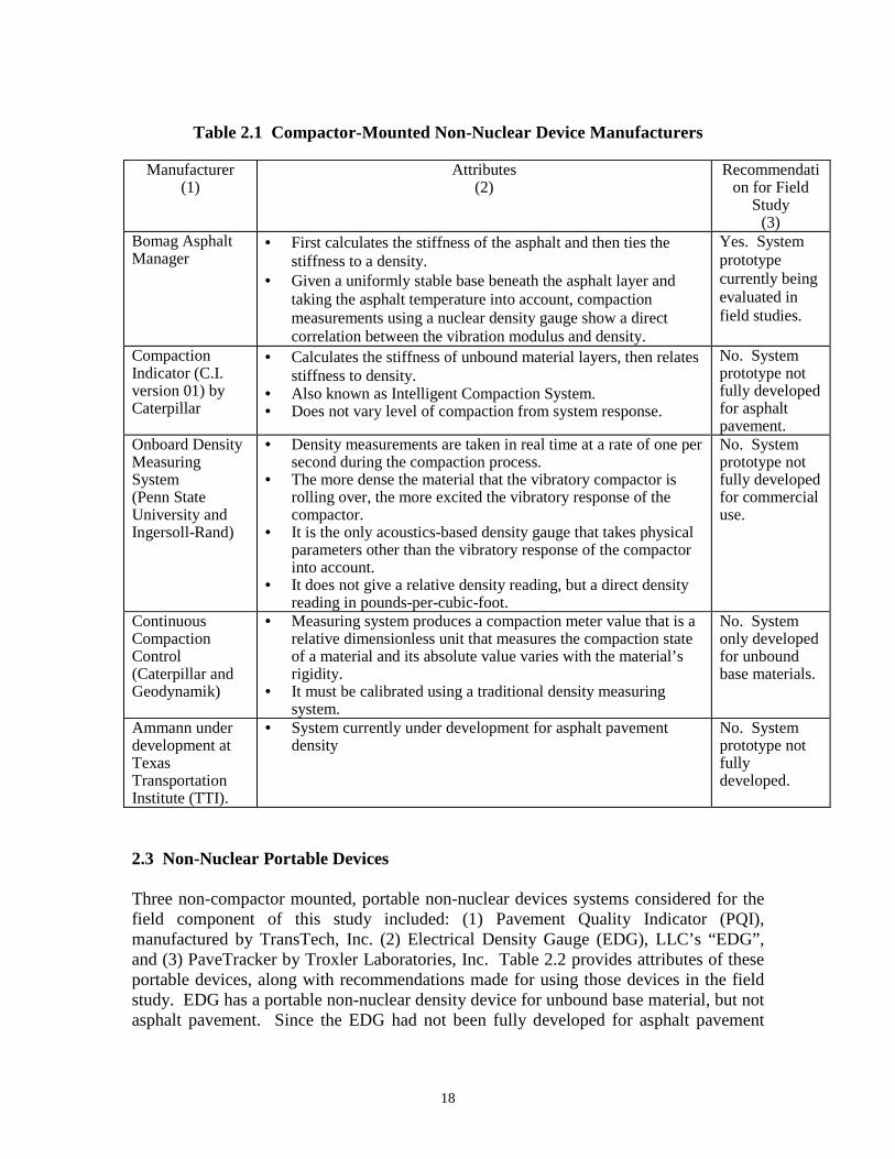
Table 2.1 Compactor-Mounted Non-Nuclear Device Manufacturers
Manufacturer (1)
Attributes (2)
Recommendati on for Field
Study (3)
Bomag Asphalt • First calculates the stiffness of the asphalt and then ties the Yes. System Manager stiffness to a density.
• Given a uniformly stable base beneath the asphalt layer and taking the asphalt temperature into account, compaction measurements using a nuclear density gauge show a direct correlation between the vibration modulus and density.
prototype currently being evaluated in field studies.
Compaction • Calculates the stiffness of unbound material layers, then relates No. System Indicator (C.I. stiffness to density. prototype not version 01) by • Also known as Intelligent Compaction System. fully developed Caterpillar • Does not vary level of compaction from system response. for asphalt
pavement. Onboard Density • Density measurements are taken in real time at a rate of one per No. System Measuring second during the compaction process. prototype not System • The more dense the material that the vibratory compactor is fully developed (Penn State rolling over, the more excited the vibratory response of the for commercial University and compactor. use. Ingersoll-Rand) • It is the only acoustics-based density gauge that takes physical
parameters other than the vibratory response of the compactor into account.
• It does not give a relative density reading, but a direct density reading in pounds-per-cubic-foot.
Continuous • Measuring system produces a compaction meter value that is a No. System Compaction relative dimensionless unit that measures the compaction state only developed Control of a material and its absolute value varies with the material’s for unbound (Caterpillar and rigidity. base materials. Geodynamik) • It must be calibrated using a traditional density measuring
system. Ammann under • System currently under development for asphalt pavement No. System development at density prototype not Texas fully Transportation developed. Institute (TTI).
2.3 Non-Nuclear Portable Devices
Three non-compactor mounted, portable non-nuclear devices systems considered for the field component of this study included: (1) Pavement Quality Indicator (PQI), manufactured by TransTech, Inc. (2) Electrical Density Gauge (EDG), LLC’s “EDG”, and (3) PaveTracker by Troxler Laboratories, Inc. Table 2.2 provides attributes of these portable devices, along with recommendations made for using those devices in the field study. EDG has a portable non-nuclear density device for unbound base material, but not asphalt pavement. Since the EDG had not been fully developed for asphalt pavement
18
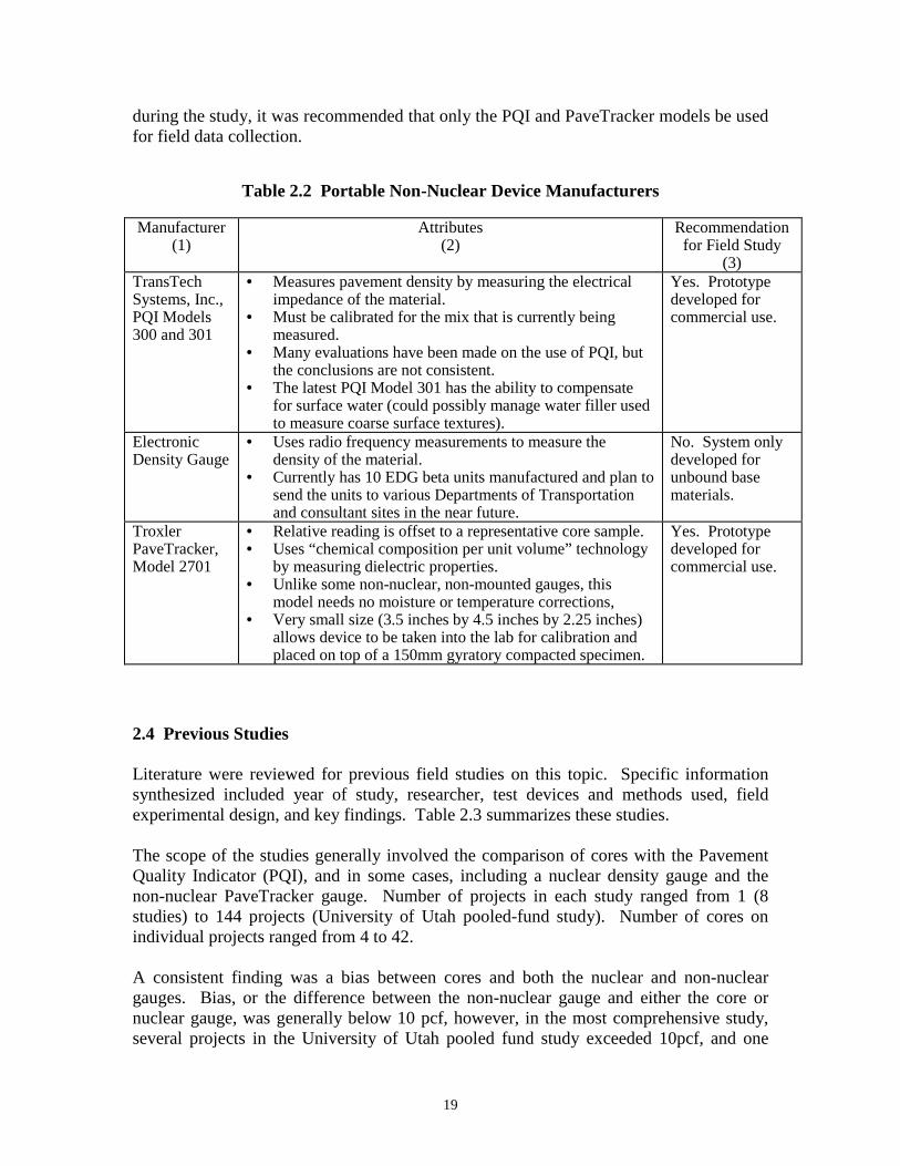
during the study, it was recommended that only the PQI and PaveTracker models be used for field data collection.
Table 2.2 Portable Non-Nuclear Device Manufacturers
Manufacturer (1)
Attributes (2)
Recommendation for Field Study
(3) TransTech Systems, Inc., PQI Models 300 and 301
• Measures pavement density by measuring the electrical impedance of the material.
• Must be calibrated for the mix that is currently being measured.
• Many evaluations have been made on the use of PQI, but the conclusions are not consistent.
• The latest PQI Model 301 has the ability to compensate for surface water (could possibly manage water filler used to measure coarse surface textures).
Yes. Prototype developed for commercial use.
Electronic • Uses radio frequency measurements to measure the No. System only Density Gauge density of the material.
• Currently has 10 EDG beta units manufactured and plan to send the units to various Departments of Transportation and consultant sites in the near future.
developed for unbound base materials.
Troxler PaveTracker, Model 2701
• Relative reading is offset to a representative core sample. • Uses “chemical composition per unit volume” technology
by measuring dielectric properties. • Unlike some non-nuclear, non-mounted gauges, this
model needs no moisture or temperature corrections, • Very small size (3.5 inches by 4.5 inches by 2.25 inches)
allows device to be taken into the lab for calibration and placed on top of a 150mm gyratory compacted specimen.
Yes. Prototype developed for commercial use.
2.4 Previous Studies
Literature were reviewed for previous field studies on this topic. Specific information synthesized included year of study, researcher, test devices and methods used, field experimental design, and key findings. Table 2.3 summarizes these studies.
The scope of the studies generally involved the comparison of cores with the Pavement Quality Indicator (PQI), and in some cases, including a nuclear density gauge and the non-nuclear PaveTracker gauge. Number of projects in each study ranged from 1 (8 studies) to 144 projects (University of Utah pooled-fund study). Number of cores on individual projects ranged from 4 to 42.
A consistent finding was a bias between cores and both the nuclear and non-nuclear gauges. Bias, or the difference between the non-nuclear gauge and either the core or nuclear gauge, was generally below 10 pcf, however, in the most comprehensive study, several projects in the University of Utah pooled fund study exceeded 10pcf, and one
19
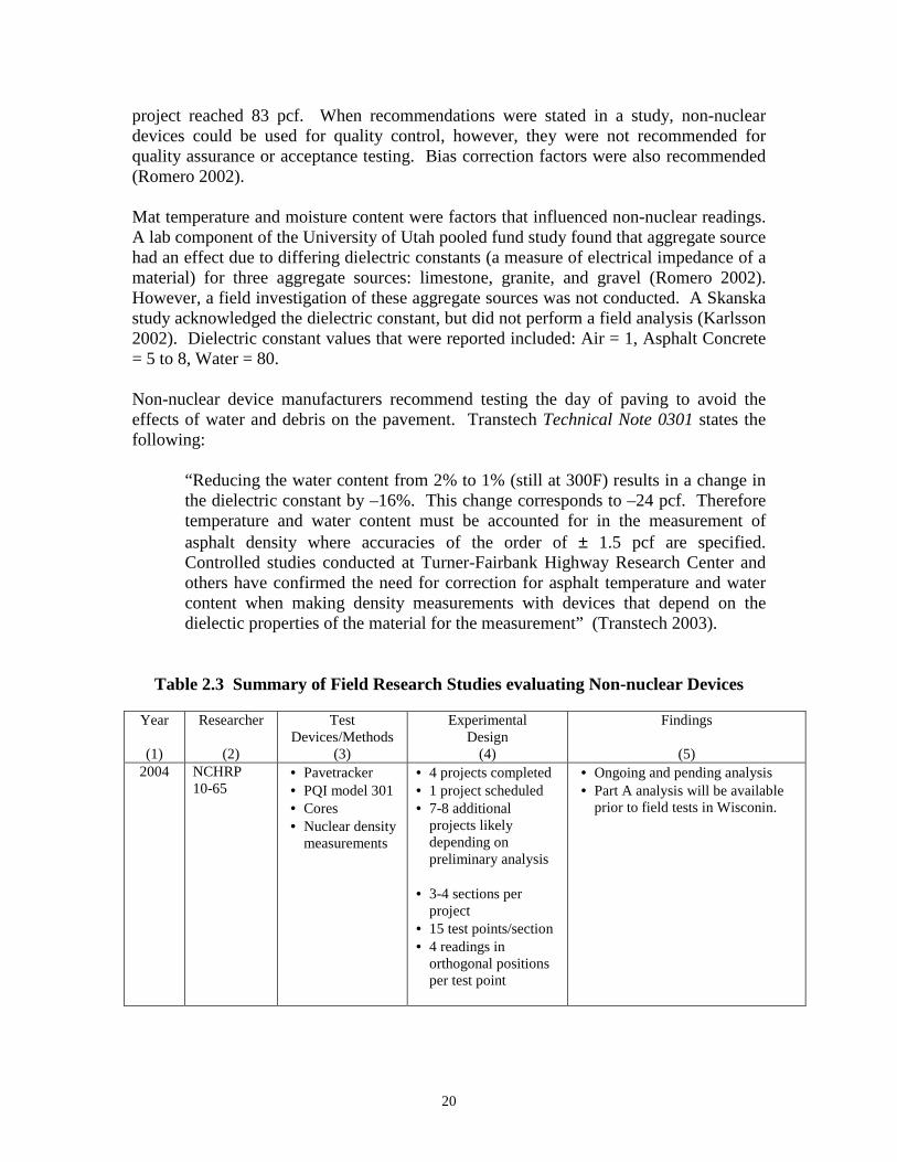
project reached 83 pcf. When recommendations were stated in a study, non-nuclear devices could be used for quality control, however, they were not recommended for quality assurance or acceptance testing. Bias correction factors were also recommended (Romero 2002).
Mat temperature and moisture content were factors that influenced non-nuclear readings. A lab component of the University of Utah pooled fund study found that aggregate source had an effect due to differing dielectric constants (a measure of electrical impedance of a material) for three aggregate sources: limestone, granite, and gravel (Romero 2002). However, a field investigation of these aggregate sources was not conducted. A Skanska study acknowledged the dielectric constant, but did not perform a field analysis (Karlsson 2002). Dielectric constant values that were reported included: Air = 1, Asphalt Concrete = 5 to 8, Water = 80.
Non-nuclear device manufacturers recommend testing the day of paving to avoid the effects of water and debris on the pavement. Transtech Technical Note 0301 states the following:
“Reducing the water content from 2% to 1% (still at 300F) results in a change in the dielectric constant by –16%. This change corresponds to –24 pcf. Therefore temperature and water content must be accounted for in the measurement of asphalt density where accuracies of the order of ± 1.5 pcf are specified. Controlled studies conducted at Turner-Fairbank Highway Research Center and others have confirmed the need for correction for asphalt temperature and water content when making density measurements with devices that depend on the dielectic properties of the material for the measurement” (Transtech 2003).
Table 2.3 Summary of Field Research Studies evaluating Non-nuclear Devices
Year
(1)
Researcher
(2)
Test Devices/Methods
(3)
Experimental Design
(4)
Findings
(5) 2004 NCHRP
10-65 • Pavetracker • PQI model 301 • Cores • Nuclear density
measurements
• 4 projects completed • 1 project scheduled • 7-8 additional
projects likely depending on preliminary analysis
• 3-4 sections per project
• 15 test points/section • 4 readings in
orthogonal positions per test point
• Ongoing and pending analysis • Part A analysis will be available
prior to field tests in Wisconin.
20
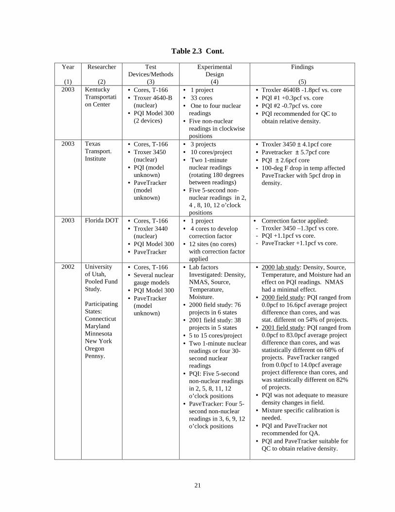
Table 2.3 Cont.
Year
(1)
Researcher
(2)
Test Devices/Methods
(3)
Experimental Design
(4)
Findings
(5) 2003 Kentucky
Transportati on Center
• Cores, T-166 • Troxer 4640-B
(nuclear) • PQI Model 300
(2 devices)
• 1 project • 33 cores • One to four nuclear
readings • Five non-nuclear
readings in clockwise positions
• Troxler 4640B -1.8pcf vs. core • PQI #1 +0.3pcf vs. core • PQI #2 -0.7pcf vs. core • PQI recommended for QC to
obtain relative density.
2003 Texas Transport. Institute
• Cores, T-166 • Troxer 3450
(nuclear) • PQI (model
unknown) • PaveTracker
(model unknown)
• 3 projects • 10 cores/project • Two 1-minute
nuclear readings (rotating 180 degrees between readings)
• Five 5-second nonnuclear readings in 2, 4 , 8, 10, 12 o’clock positions
• Troxler 3450 ± 4.1pcf core • Pavetracker ± 5.7pcf core • PQI ± 2.6pcf core • 100-deg F drop in temp affected
PaveTracker with 5pcf drop in density.
2003 Florida DOT • Cores, T-166 • Troxler 3440
(nuclear) • PQI Model 300 • PaveTracker
• 1 project • 4 cores to develop
correction factor • 12 sites (no cores)
with correction factor applied
• Correction factor applied: - Troxler 3450 –1.3pcf vs core. - PQI +1.1pcf vs core. - PaveTracker +1.1pcf vs core.
2002 University of Utah, Pooled Fund Study.
Participating States: Connecticut Maryland Minnesota New York Oregon Pennsy.
• Cores, T-166 • Several nuclear
gauge models • PQI Model 300 • PaveTracker
(model unknown)
• Lab factors Investigated: Density, NMAS, Source, Temperature, Moisture.
• 2000 field study: 76 projects in 6 states
• 2001 field study: 38 projects in 5 states
• 5 to 15 cores/project • Two 1-minute nuclear
readings or four 30second nuclear readings
• PQI: Five 5-second non-nuclear readings in 2, 5, 8, 11, 12 o’clock positions
• PaveTracker: Four 5second non-nuclear readings in 3, 6, 9, 12 o’clock positions
• 2000 lab study: Density, Source, Temperature, and Moisture had an effect on PQI readings. NMAS had a minimal effect.
• 2000 field study: PQI ranged from 0.0pcf to 16.6pcf average project difference than cores, and was stat. different on 54% of projects.
• 2001 field study: PQI ranged from 0.0pcf to 83.0pcf average project difference than cores, and was statistically different on 68% of projects. PaveTracker ranged from 0.0pcf to 14.0pcf average project difference than cores, and was statistically different on 82% of projects.
• PQI was not adequate to measure density changes in field.
• Mixture specific calibration is needed.
• PQI and PaveTracker not recommended for QA.
• PQI and PaveTracker suitable for QC to obtain relative density.
21
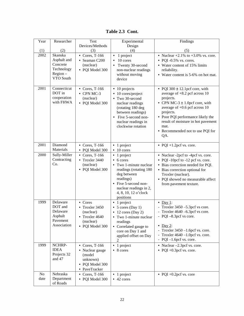
Table 2.3 Cont.
Year
(1)
Researcher
(2)
Test Devices/Methods
(3)
Experimental Design
(4)
Findings
(5) 2002 Skanska
Asphalt and Concrete Technology Region – VTO South
• Cores, T-166 • Seaman C200
(nuclear) • PQI Model 300
• 1 project • 10 cores • Twenty 30-second
non-nuclear readings without moving device
• Nuclear +2.1% to +3.0% vs. core. • PQI -0.5% vs. cores. • Water content of 15% limits
reliability. • Water content is 5-6% on hot mat.
2001 Connecticut DOT in cooperation with FHWA
• Cores, T-166 • CPN MC-3
(nuclear) • PQI Model 300
• 10 projects • 10 cores/project • Two 30-second
nuclear readings (rotating 180 deg between readings)
• Five 5-second nonnuclear readings in clockwise rotation
• PQI 300 ± 12.1pcf core, with average of +8.2 pcf across 10 projects.
• CPN MC-3 ± 1.0pcf core, with average of +0.6 pcf across 10 projects.
• Poor PQI performance likely the result of moisture in hot pavement mat.
• Recommended not to use PQI for QA.
2001 Diamond Materials
• Cores, T-166 • PQI Model 300
• 1 project • 10 cores
• PQI +1.2pcf vs. core.
2000 Sully-Miller Contracting Co.
• Cores, T-166 • Troxler 3440
(nuclear) • PQI Model 300
• 1 project • 6 cores • Two 1-minute nuclear
readings (rotating 180 deg between readings)
• Five 5-second nonnuclear readings in 2, 4, 8, 10, 12 o’clock positions
• Nuclear -2pcf to -4pcf vs. core. • PQI -10pcf to -12 pcf vs. core. • Bias correction needed for PQI. • Bias correction optional for
Troxler (nuclear). • PQI showed no measurable affect
from pavement texture.
1999 Delaware DOT and Delaware Asphalt Pavement Association
• Cores • Troxler 3450
(nuclear) • Troxler 4640
(nuclear) • PQI Model 300
• 1 project • 5 cores (Day 1) • 12 cores (Day 2) • Two 1-minute nuclear
readings • Correlated gauge to
core on Day 1 and applied offset on Day 2
• Day 1: - Troxler 3450 –5.3pcf vs core. - Troxler 4640 –6.3pcf vs core. - PQI –8.3pcf vs core.
• Day 2: - Troxler 3450 –1.6pcf vs. core. - Troxler 4640 –1.0pcf vs. core. - PQI –1.6pcf vs. core.
1999 NCHRPIDEA Projects 32 and 47
• Cores, T-166 • Nuclear gauge
(model unknown)
• PQI Model 300 • PaveTracker
• 1 project • 8 cores
• Nuclear –2.3pcf vs. core. • PQI +0.3pcf vs. core.
No date
Nebraska Department of Roads
• Cores, T-166 • PQI Model 300
• 1 project • 42 cores
• PQI +0.2pcf vs. core
22
CHAPTER 3 EXPERIMENTAL DESIGN
3.1 Introduction
In the previous chapter, a critical review of non-nuclear devices recommended the following for the field study: (1) Bomag Asphalt Manager and Bomag VarioControl Compactor, a compactor-mounted system manufactured by Bomag, (2) Pavement Quality Indicator (PQI) manufactured by TransTech Systems, Inc., and (3) PaveTracker manufactured by Troxler Laboratories, Inc. An attempt was made to schedule the Bomag prototype system on at least one field project for this study; however, there were schedule conflicts and previous commitments in other states. From this list, a field experimental design, or work plan, was developed to collect in-place density data from actual construction projects.
3.2 Work Plan Parameters
The work plan incorporated findings from several sources, including: (1) the literature review, (2) on-going NCHRP Project #10-65, (3) meeting with WHRP Project Oversight Committee (panel) on November 30, 2004, and (4) meeting with the research team on January 11, 2005. A work plan was submitted to the WHRP Panel on April 6, 2005, and comments from the panel were incorporated into the finalized plan dated May 10, 2005. Key parameters for the work plan are detailed in the following sections.
3.2.1 Test Equipment
Two portable non-nuclear manufacturers/models were initially specified for the field study: (1) TransTech PQI Model 301, and (2) Troxler PaveTracker Model 2701b. These model numbers were the latest devices from both manufacturers. Payne and Dolan, Inc., furnished their PQI Model 300 non-nuclear density gauge on Projects #6 through #16. Test procedures for both manufacturers were followed, in particular, five readings in the region of the where the core or nuclear density readings were taken. Six-inch diameter core bit and CPN MC-3 nuclear density gauge were also used.
The PaveTracker gauge was checked for calibration to the manufacturer’s glass reference block in the carrying case before and after testing each day. If the gauge was turned off during the day to save battery power, the reference block was retested and the readings were always within ± 0.2 pcf of the 151.0 pcf reference block density.
PQI models were not calibrated to any block or device throughout field testing. The manufacturer provides no reference block, but suggests that standard project calibration data be entered before daily field testing. These entries included the layer (intermediate or surface), NMAS, and lift thickness. If any moisture readings exceeded an indexed value of 10, the machine should be checked, or another site be tested.
23
3.2.2 Projects
The proposed April 6th work plan was to collect data from 16 projects; 12 Superpave projects and 4 SMA projects. The project panel recommended that resources be used to test more than 12 Superpave projects, and proportionally reduce the number of SMA projects. The reason for this recommendation was that SMA will most likely have a different test protocol than Superpave, which could be developed at a later date. Thus, 16 Superpave projects were specified for data collection.
Three source aggregates, two base types, and two replicates of each source/base combination were initially proposed, yielding a total of 12 projects (3 x 2 x 2). Source aggregate types included gravel, granite, and limestone. Base types included PCC, HMA, and CABC. The remaining four projects were considered additional replicates. During field data collection, it was not possible to identify projects with the desired source/base combination, and as a result, priority was given to aggregate source type. This decision was based upon the literature review, where a lab study by the University of Utah found that aggregate source affected non-nuclear density readings (Romero 2002). None of the previous studies evaluated base type, however, and the decision was made to use pavement layer thickness as a surrogate variable for base effects.
3.2.3 Test Sites
Thirty (30) QA comparison test sites after finish rolling were randomly chosen on each project for collecting comparison data between cores, nuclear density gauge, and both PQI and PaveTracker non-nuclear gauges.
Five (5) QC test sites were selectively determined on each project to compare the nuclear gauge and both the PQI and PaveTracker non-nuclear gauges during compaction operations. Density and temperature readings were taken behind the paver screed and after series of roller passes until final compaction. This data allowed an assessment of gauge response under changing temperature and density conditions, and whether the devices are robust to this environment.
The project panel recommended not using surface fillers (sand, gels, water, etc.) in the field study. There was no standardized procedure to apply fillers to the surface (volume, weight, surface area, time allotment, etc.), and appropriate filler materials have not been clearly defined. In addition, non-nuclear devices are very sensitive to water since they use electrical impedance to determine material density.
24
3.2.4 Cores
The most significant change between the April 6th and May 10th work plans was the reduction of number of cores per project from 20 to 10, and increase of nuclear density readings from 20 to 30. The project panel preferred the use of the nuclear density gauge as the baseline for non-nuclear density readings, and cores as a simple check on the nuclear density gauge readings.
The WHRP panel recommended that WisDOT Method 1559 (modified AASHTO T-166) be used to test density on all core samples, as opposed to Corelok testing. Corelok has several distinct advantages, such as improved accuracy of core density and minimal repeatability error. By limiting the study to WisDOT Method 1559, normal variability and bias would be built into the data set. In addition, limited resources were to be spent on collecting more field data, rather than performing on both Corelok and Method 1559 testing in the lab.
25
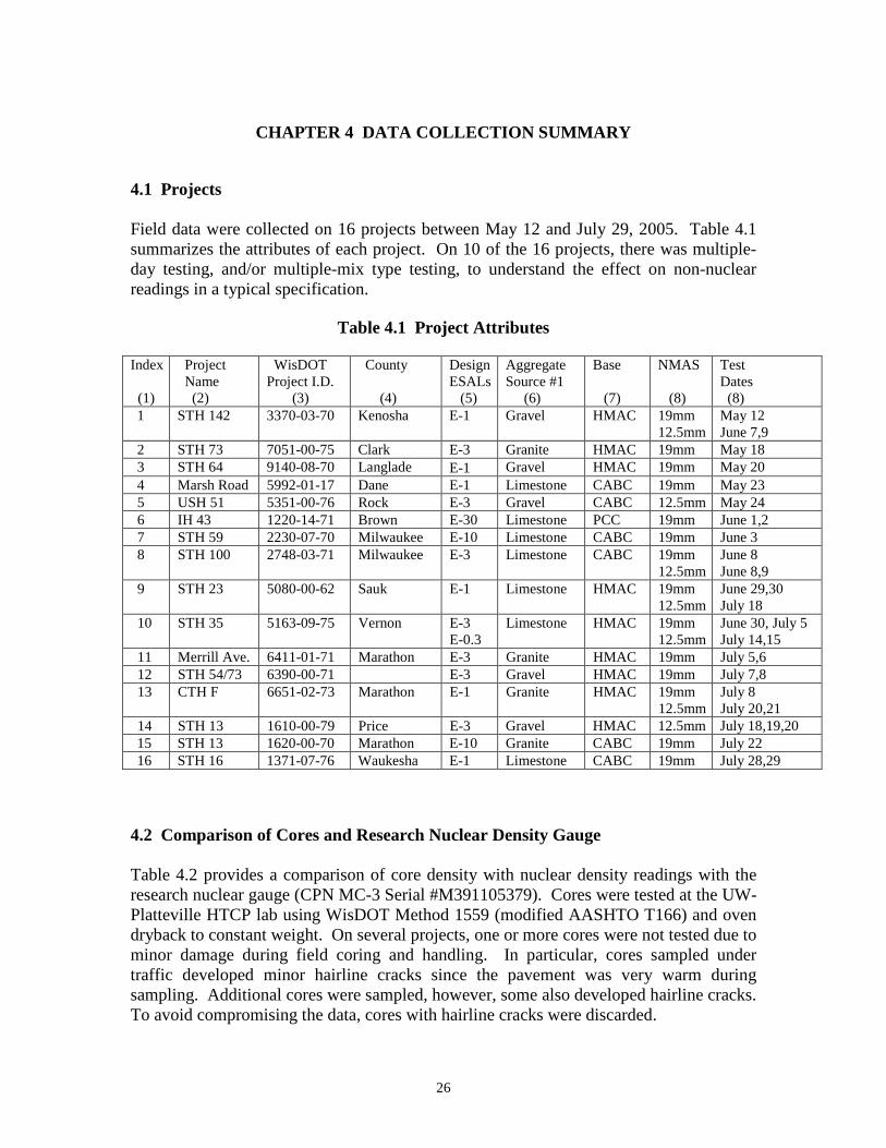
CHAPTER 4 DATA COLLECTION SUMMARY
4.1 Projects
Field data were collected on 16 projects between May 12 and July 29, 2005. Table 4.1 summarizes the attributes of each project. On 10 of the 16 projects, there was multiple-day testing, and/or multiple-mix type testing, to understand the effect on non-nuclear readings in a typical specification.
Table 4.1 Project Attributes
Index
(1)
Project Name
(2)
WisDOT Project I.D.
(3)
County
(4)
Design ESALs
(5)
Aggregate Source #1
(6)
Base
(7)
NMAS
(8)
Test Dates
(8) 1 STH 142 3370-03-70 Kenosha E-1 Gravel HMAC 19mm
12.5mm May 12 June 7,9
2 STH 73 7051-00-75 Clark E-3 Granite HMAC 19mm May 18 3 STH 64 9140-08-70 Langlade E-1 Gravel HMAC 19mm May 20 4 Marsh Road 5992-01-17 Dane E-1 Limestone CABC 19mm May 23 5 USH 51 5351-00-76 Rock E-3 Gravel CABC 12.5mm May 24 6 IH 43 1220-14-71 Brown E-30 Limestone PCC 19mm June 1,2 7 STH 59 2230-07-70 Milwaukee E-10 Limestone CABC 19mm June 3 8 STH 100 2748-03-71 Milwaukee E-3 Limestone CABC 19mm
12.5mm June 8 June 8,9
9 STH 23 5080-00-62 Sauk E-1 Limestone HMAC 19mm 12.5mm
June 29,30 July 18
10 STH 35 5163-09-75 Vernon E-3 E-0.3
Limestone HMAC 19mm 12.5mm
June 30, July 5 July 14,15
11 Merrill Ave. 6411-01-71 Marathon E-3 Granite HMAC 19mm July 5,6 12 STH 54/73 6390-00-71 E-3 Gravel HMAC 19mm July 7,8 13 CTH F 6651-02-73 Marathon E-1 Granite HMAC 19mm
12.5mm July 8 July 20,21
14 STH 13 1610-00-79 Price E-3 Gravel HMAC 12.5mm July 18,19,20 15 STH 13 1620-00-70 Marathon E-10 Granite CABC 19mm July 22 16 STH 16 1371-07-76 Waukesha E-1 Limestone CABC 19mm July 28,29
4.2 Comparison of Cores and Research Nuclear Density Gauge
Table 4.2 provides a comparison of core density with nuclear density readings with the research nuclear gauge (CPN MC-3 Serial #M391105379). Cores were tested at the UW-Platteville HTCP lab using WisDOT Method 1559 (modified AASHTO T166) and oven dryback to constant weight. On several projects, one or more cores were not tested due to minor damage during field coring and handling. In particular, cores sampled under traffic developed minor hairline cracks since the pavement was very warm during sampling. Additional cores were sampled, however, some also developed hairline cracks. To avoid compromising the data, cores with hairline cracks were discarded.
26
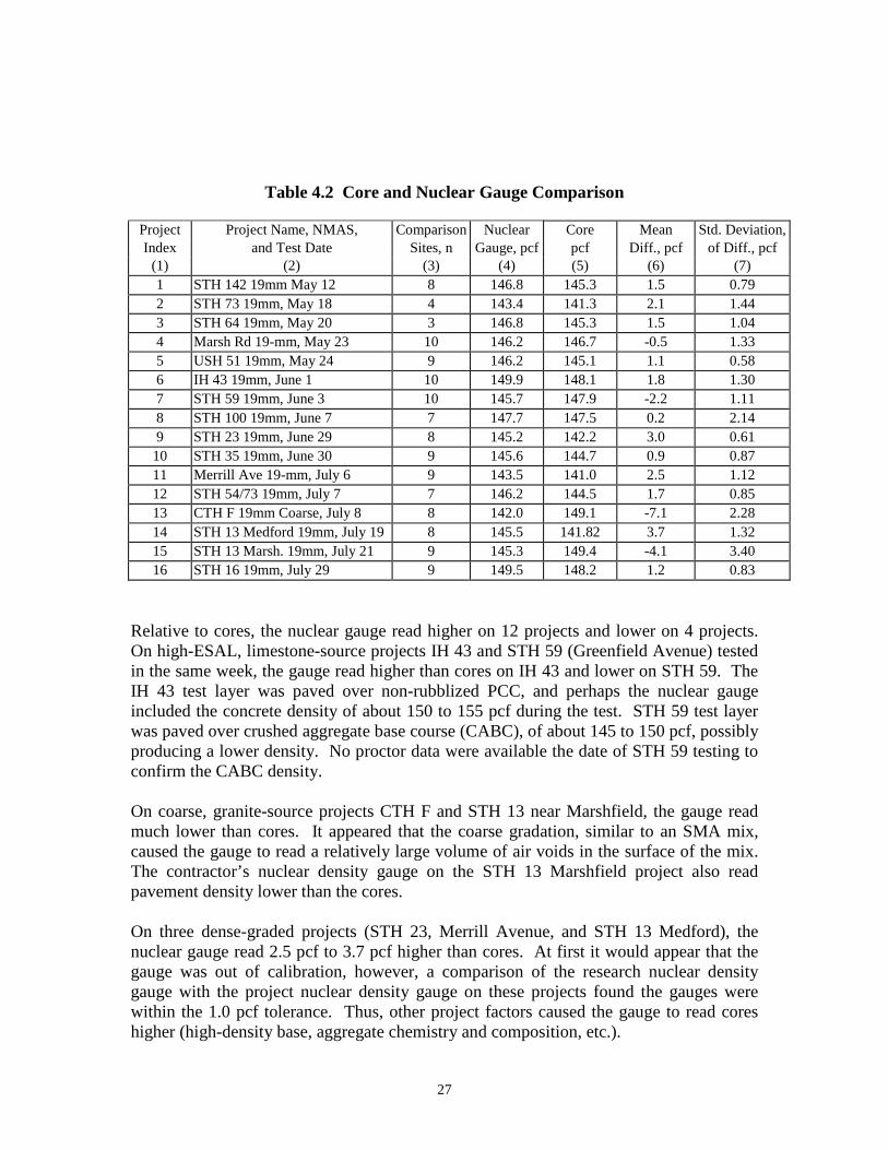
Table 4.2 Core and Nuclear Gauge Comparison
Project Index
(1)
Project Name, NMAS, and Test Date
(2)
Comparison Sites, n
(3)
Nuclear Gauge, pcf
(4)
Core pcf (5)
Mean Diff., pcf
(6)
Std. Deviation, of Diff., pcf
(7) 1 STH 142 19mm May 12 8 146.8 145.3 1.5 0.79 2 STH 73 19mm, May 18 4 143.4 141.3 2.1 1.44 3 STH 64 19mm, May 20 3 146.8 145.3 1.5 1.04 4 Marsh Rd 19-mm, May 23 10 146.2 146.7 -0.5 1.33 5 USH 51 19mm, May 24 9 146.2 145.1 1.1 0.58 6 IH 43 19mm, June 1 10 149.9 148.1 1.8 1.30 7 STH 59 19mm, June 3 10 145.7 147.9 -2.2 1.11 8 STH 100 19mm, June 7 7 147.7 147.5 0.2 2.14 9 STH 23 19mm, June 29 8 145.2 142.2 3.0 0.61
10 STH 35 19mm, June 30 9 145.6 144.7 0.9 0.87 11 Merrill Ave 19-mm, July 6 9 143.5 141.0 2.5 1.12 12 STH 54/73 19mm, July 7 7 146.2 144.5 1.7 0.85 13 CTH F 19mm Coarse, July 8 8 142.0 149.1 -7.1 2.28 14 STH 13 Medford 19mm, July 19 8 145.5 141.82 3.7 1.32 15 STH 13 Marsh. 19mm, July 21 9 145.3 149.4 -4.1 3.40 16 STH 16 19mm, July 29 9 149.5 148.2 1.2 0.83
Relative to cores, the nuclear gauge read higher on 12 projects and lower on 4 projects. On high-ESAL, limestone-source projects IH 43 and STH 59 (Greenfield Avenue) tested in the same week, the gauge read higher than cores on IH 43 and lower on STH 59. The IH 43 test layer was paved over non-rubblized PCC, and perhaps the nuclear gauge included the concrete density of about 150 to 155 pcf during the test. STH 59 test layer was paved over crushed aggregate base course (CABC), of about 145 to 150 pcf, possibly producing a lower density. No proctor data were available the date of STH 59 testing to confirm the CABC density.
On coarse, granite-source projects CTH F and STH 13 near Marshfield, the gauge read much lower than cores. It appeared that the coarse gradation, similar to an SMA mix, caused the gauge to read a relatively large volume of air voids in the surface of the mix. The contractor’s nuclear density gauge on the STH 13 Marshfield project also read pavement density lower than the cores.
On three dense-graded projects (STH 23, Merrill Avenue, and STH 13 Medford), the nuclear gauge read 2.5 pcf to 3.7 pcf higher than cores. At first it would appear that the gauge was out of calibration, however, a comparison of the research nuclear density gauge with the project nuclear density gauge on these projects found the gauges were within the 1.0 pcf tolerance. Thus, other project factors caused the gauge to read cores higher (high-density base, aggregate chemistry and composition, etc.).
27
4.3 Comparison of Nuclear Density Gauges
On each project, the research nuclear gauge compared readings with the project nuclear gauge (WisDOT and/or contractor) at the comparative test sites. Standard 4-minute test readings were taken. Comparative readings were taken on both QMP sites and randomly-chosen sites for the study, thus, the number of data points per project varied. Mr. Bob Schiro, WisDOT Radiation Safety Officer, was invited to test on all projects to ensure compliance with QMP test procedures, and to provide additional research data. He was able to provide data for 27 test sites on the STH 142 project (May 12th).
Table 4.3 summarizes the averages with each gauge for the same sites tested, along with the mean and standard deviation of their difference. The results suggest that gauges were at or near the tolerance of 1.0 pcf on most projects. Different gauges (same model and different serial number) were used by the contractor on the IH 43 and STH 100 (Ryan Road) projects, and the mean difference changed between test days.
The contractor’s nuclear density gauge on the STH 13 Marshfield project was an average of 2.1 pcf lower than the research nuclear density gauge. As noted earlier, this mix was coarse graded, and it may have caused problems with the backscatter procedure to determine density.
28
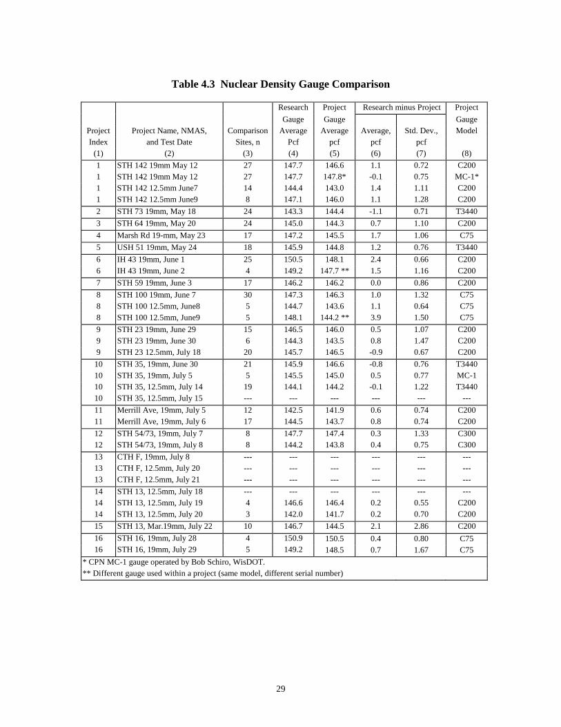
Table 4.3 Nuclear Density Gauge Comparison
Project Index
(1)
Project Name, NMAS, and Test Date
(2)
Comparison Sites, n
(3)
Research
Gauge Average
Pcf (4)
Project
Gauge Average
pcf (5)
Research minus Project Project
Gauge Model
(8)
Average, pcf (6)
Std. Dev., pcf (7)
1 1 1 1
STH 142 19mm May 12 STH 142 19mm May 12 STH 142 12.5mm June7 STH 142 12.5mm June9
27 27 14 8
147.7 147.7 144.4 147.1
146.6 147.8* 143.0 146.0
1.1 -0.1 1.4 1.1
0.72 0.75 1.11 1.28
C200 MC-1* C200 C200
2 STH 73 19mm, May 18 24 143.3 144.4 -1.1 0.71 T3440
3 STH 64 19mm, May 20 24 145.0 144.3 0.7 1.10 C200
4 Marsh Rd 19-mm, May 23 17 147.2 145.5 1.7 1.06 C75
5 USH 51 19mm, May 24 18 145.9 144.8 1.2 0.76 T3440
6 6
IH 43 19mm, June 1 IH 43 19mm, June 2
25 4
150.5 149.2
148.1 147.7 **
2.4 1.5
0.66 1.16
C200 C200
7 STH 59 19mm, June 3 17 146.2 146.2 0.0 0.86 C200
8 8 8
STH 100 19mm, June 7 STH 100 12.5mm, June8 STH 100 12.5mm, June9
30 5 5
147.3 144.7 148.1
146.3 143.6
144.2 **
1.0 1.1 3.9
1.32 0.64 1.50
C75 C75 C75
9 9 9
STH 23 19mm, June 29 STH 23 19mm, June 30 STH 23 12.5mm, July 18
15 6
20
146.5 144.3 145.7
146.0 143.5 146.5
0.5 0.8 -0.9
1.07 1.47 0.67
C200 C200 C200
10 10 10 10
STH 35, 19mm, June 30 STH 35, 19mm, July 5 STH 35, 12.5mm, July 14 STH 35, 12.5mm, July 15
21 5
19 --
145.9 145.5 144.1
--
146.6 145.0 144.2
--
-0.8 0.5 -0.1 --
0.76 0.77 1.22 --
T3440 MC-1 T3440
--
11 11
Merrill Ave, 19mm, July 5 Merrill Ave, 19mm, July 6
12 17
142.5 144.5
141.9 143.7
0.6 0.8
0.74 0.74
C200 C200
12 12
STH 54/73, 19mm, July 7 STH 54/73, 19mm, July 8
8 8
147.7 144.2
147.4 143.8
0.3 0.4
1.33 0.75
C300 C300
13 13 13
CTH F, 19mm, July 8 CTH F, 12.5mm, July 20 CTH F, 12.5mm, July 21
------
------
------
------
------
------
14 14 14
STH 13, 12.5mm, July 18 STH 13, 12.5mm, July 19 STH 13, 12.5mm, July 20
--4 3
--146.6 142.0
--146.4 141.7
--0.2 0.2
--0.55 0.70
--C200 C200
15 STH 13, Mar.19mm, July 22 10 146.7 144.5 2.1 2.86 C200
16 16
STH 16, 19mm, July 28 STH 16, 19mm, July 29
4 5
150.9 149.2
150.5 148.5
0.4 0.7
0.80 1.67
C75 C75
* CPN MC-1 gauge operated by Bob Schiro, WisDOT. ** Different gauge used within a project (same model, different serial number)
29

4.4 Comparison of Nuclear and Non-Nuclear Density Gauges
Table 4.4 provides a comparison of average non-nuclear density readings with the research nuclear gauge (CPN MC-3 Serial #M391105379). Nuclear readings were obtained with a standard 4-minute test, and non-nuclear gauges used the average of 5 cluster points (1 at the center, and 4 corner points at the rectangular nuclear density gauge base).
The field study began using the CPN MC-3 nuclear gauge, PQI 301, and PaveTracker 2701B. On June 1, Payne & Dolan allowed the research team to use their PQI Model #300, beginning with the IH 43 project. Then on June 3 at the start of testing on the STH 59 project, the PQI Model #301 had an electrical failure and was not operable. A replacement gauge was sent the following week for testing on the STH 142 and STH 100 projects, however, the replacement gauge also suffered an electrical failure. The replacement was sent back to Transtech, and the original PQI Model #301 was repaired and sent back to the research team, with testing resuming on the STH 23 and STH 35 projects. Empty cells in Table 4.4 indicate the gauge was not operated on the given project.
A consistent finding was a bias between nuclear and non-nuclear gauges, and a change in bias within a project between days or a different mix type. All non-nuclear models consistently read lower than the nuclear gauge. PQI Model #301 consistently read 11.2 to 27.2 pcf lower than the nuclear gauge, while PQI Model #300 ranged from 4.2 to 26.6 pcf lower. PaveTracker varied from 1.8 to 17.7 pcf.
Within a project, the bias varied between the nuclear gauge and each of the non-nuclear gauges. For example, on the STH 142 12.5-mm mat, the bias with the PQI Model #300 varied from 9.4 pcf to 15.9 pcf between June 7 and 9, respectively. For the same dates, the Pavetracker bias was 7.2 pcf and 6.5 pcf.
30
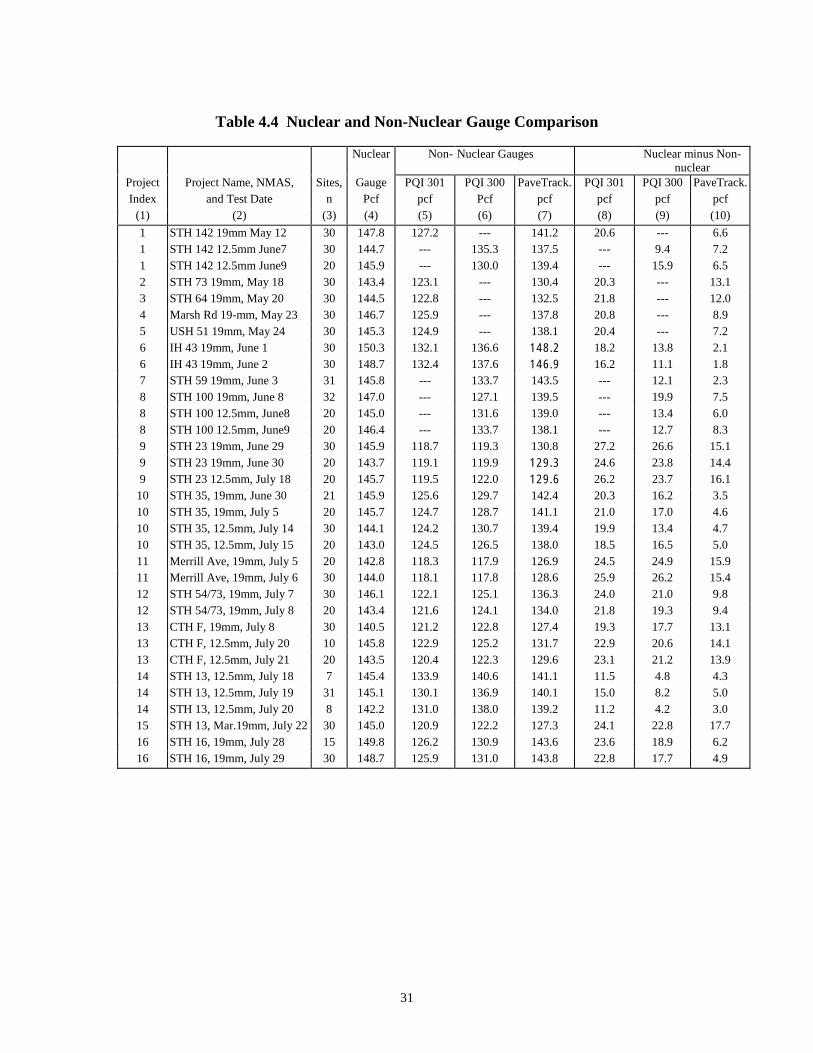
Table 4.4 Nuclear and Non-Nuclear Gauge Comparison
Project Project Name, NMAS, Sites,
Nuclear
Gauge
Non- Nuclear Gauges Nuclear minus Nonnuclear
PQI 301 PQI 300 PaveTrack. PQI 301 PQI 300 PaveTrack. Index and Test Date n Pcf pcf Pcf pcf pcf pcf pcf
(1) (2) (3) (4) (5) (6) (7) (8) (9) (10)
1 STH 142 19mm May 12 30 147.8 127.2 -- 141.2 20.6 -- 6.6 1 STH 142 12.5mm June7 30 144.7 -- 135.3 137.5 -- 9.4 7.2 1 STH 142 12.5mm June9 20 145.9 -- 130.0 139.4 -- 15.9 6.5 2 STH 73 19mm, May 18 30 143.4 123.1 -- 130.4 20.3 -- 13.1 3 STH 64 19mm, May 20 30 144.5 122.8 -- 132.5 21.8 -- 12.0 4 Marsh Rd 19-mm, May 23 30 146.7 125.9 -- 137.8 20.8 -- 8.9 5 USH 51 19mm, May 24 30 145.3 124.9 -- 138.1 20.4 -- 7.2 6 IH 43 19mm, June 1 30 150.3 132.1 136.6 148.2 18.2 13.8 2.1 6 IH 43 19mm, June 2 30 148.7 132.4 137.6 146.9 16.2 11.1 1.8 7 STH 59 19mm, June 3 31 145.8 -- 133.7 143.5 -- 12.1 2.3 8 STH 100 19mm, June 8 32 147.0 -- 127.1 139.5 -- 19.9 7.5 8 STH 100 12.5mm, June8 20 145.0 -- 131.6 139.0 -- 13.4 6.0 8 STH 100 12.5mm, June9 20 146.4 -- 133.7 138.1 -- 12.7 8.3 9 STH 23 19mm, June 29 30 145.9 118.7 119.3 130.8 27.2 26.6 15.1 9 STH 23 19mm, June 30 20 143.7 119.1 119.9 129.3 24.6 23.8 14.4 9 STH 23 12.5mm, July 18 20 145.7 119.5 122.0 129.6 26.2 23.7 16.1
10 STH 35, 19mm, June 30 21 145.9 125.6 129.7 142.4 20.3 16.2 3.5 10 STH 35, 19mm, July 5 20 145.7 124.7 128.7 141.1 21.0 17.0 4.6 10 STH 35, 12.5mm, July 14 30 144.1 124.2 130.7 139.4 19.9 13.4 4.7 10 STH 35, 12.5mm, July 15 20 143.0 124.5 126.5 138.0 18.5 16.5 5.0 11 Merrill Ave, 19mm, July 5 20 142.8 118.3 117.9 126.9 24.5 24.9 15.9 11 Merrill Ave, 19mm, July 6 30 144.0 118.1 117.8 128.6 25.9 26.2 15.4 12 STH 54/73, 19mm, July 7 30 146.1 122.1 125.1 136.3 24.0 21.0 9.8 12 STH 54/73, 19mm, July 8 20 143.4 121.6 124.1 134.0 21.8 19.3 9.4 13 CTH F, 19mm, July 8 30 140.5 121.2 122.8 127.4 19.3 17.7 13.1 13 CTH F, 12.5mm, July 20 10 145.8 122.9 125.2 131.7 22.9 20.6 14.1 13 CTH F, 12.5mm, July 21 20 143.5 120.4 122.3 129.6 23.1 21.2 13.9 14 STH 13, 12.5mm, July 18 7 145.4 133.9 140.6 141.1 11.5 4.8 4.3 14 STH 13, 12.5mm, July 19 31 145.1 130.1 136.9 140.1 15.0 8.2 5.0 14 STH 13, 12.5mm, July 20 8 142.2 131.0 138.0 139.2 11.2 4.2 3.0 15 STH 13, Mar.19mm, July 22 30 145.0 120.9 122.2 127.3 24.1 22.8 17.7 16 STH 16, 19mm, July 28 15 149.8 126.2 130.9 143.6 23.6 18.9 6.2 16 STH 16, 19mm, July 29 30 148.7 125.9 131.0 143.8 22.8 17.7 4.9
31
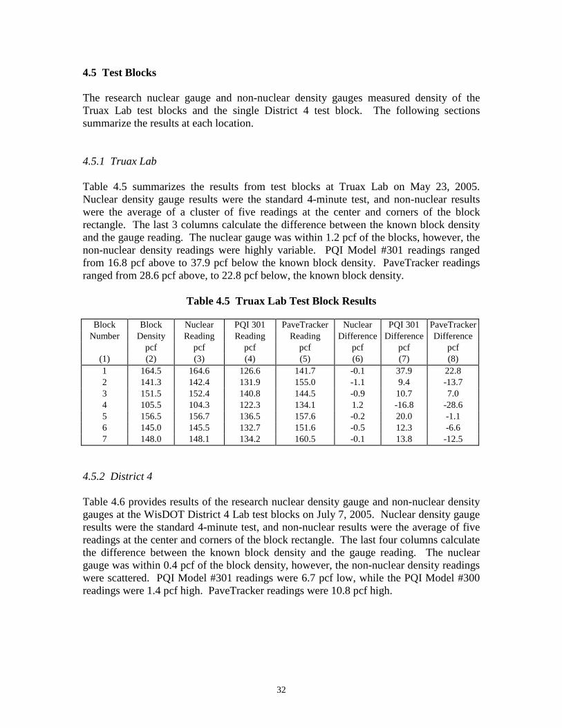
4.5 Test Blocks
The research nuclear gauge and non-nuclear density gauges measured density of the Truax Lab test blocks and the single District 4 test block. The following sections summarize the results at each location.
4.5.1 Truax Lab
Table 4.5 summarizes the results from test blocks at Truax Lab on May 23, 2005. Nuclear density gauge results were the standard 4-minute test, and non-nuclear results were the average of a cluster of five readings at the center and corners of the block rectangle. The last 3 columns calculate the difference between the known block density and the gauge reading. The nuclear gauge was within 1.2 pcf of the blocks, however, the non-nuclear density readings were highly variable. PQI Model #301 readings ranged from 16.8 pcf above to 37.9 pcf below the known block density. PaveTracker readings ranged from 28.6 pcf above, to 22.8 pcf below, the known block density.
Table 4.5 Truax Lab Test Block Results
Block Block Nuclear PQI 301 PaveTracker Nuclear PQI 301 PaveTracker Number Density Reading Reading Reading Difference Difference Difference
pcf pcf pcf pcf pcf pcf pcf (1) (2) (3) (4) (5) (6) (7) (8) 1 164.5 164.6 126.6 141.7 -0.1 37.9 22.8 2 141.3 142.4 131.9 155.0 -1.1 9.4 -13.7 3 151.5 152.4 140.8 144.5 -0.9 10.7 7.0 4 105.5 104.3 122.3 134.1 1.2 -16.8 -28.6 5 156.5 156.7 136.5 157.6 -0.2 20.0 -1.1 6 145.0 145.5 132.7 151.6 -0.5 12.3 -6.6 7 148.0 148.1 134.2 160.5 -0.1 13.8 -12.5
4.5.2 District 4
Table 4.6 provides results of the research nuclear density gauge and non-nuclear density gauges at the WisDOT District 4 Lab test blocks on July 7, 2005. Nuclear density gauge results were the standard 4-minute test, and non-nuclear results were the average of five readings at the center and corners of the block rectangle. The last four columns calculate the difference between the known block density and the gauge reading. The nuclear gauge was within 0.4 pcf of the block density, however, the non-nuclear density readings were scattered. PQI Model #301 readings were 6.7 pcf low, while the PQI Model #300 readings were 1.4 pcf high. PaveTracker readings were 10.8 pcf high.
32
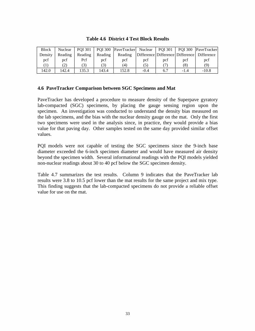
Table 4.6 District 4 Test Block Results
Block Density
pcf (1)
Nuclear Reading
pcf (2)
PQI 301 Reading
Pcf (3)
PQI 300 Reading
pcf (3)
PaveTracker Reading
pcf (4)
Nuclear Difference
pcf (5)
PQI 301 Difference
pcf (7)
PQI 300 Difference
pcf (8)
PaveTracker Difference
pcf (9)
142.0 142.4 135.3 143.4 152.8 -0.4 6.7 -1.4 -10.8
4.6 PaveTracker Comparison between SGC Specimens and Mat
PaveTracker has developed a procedure to measure density of the Superpave gyratory lab-compacted (SGC) specimens, by placing the gauge sensing region upon the specimen. An investigation was conducted to understand the density bias measured on the lab specimens, and the bias with the nuclear density gauge on the mat. Only the first two specimens were used in the analysis since, in practice, they would provide a bias value for that paving day. Other samples tested on the same day provided similar offset values.
PQI models were not capable of testing the SGC specimens since the 9-inch base diameter exceeded the 6-inch specimen diameter and would have measured air density beyond the specimen width. Several informational readings with the PQI models yielded non-nuclear readings about 30 to 40 pcf below the SGC specimen density.
Table 4.7 summarizes the test results. Column 9 indicates that the PaveTracker lab results were 3.8 to 10.5 pcf lower than the mat results for the same project and mix type. This finding suggests that the lab-compacted specimens do not provide a reliable offset value for use on the mat.
33
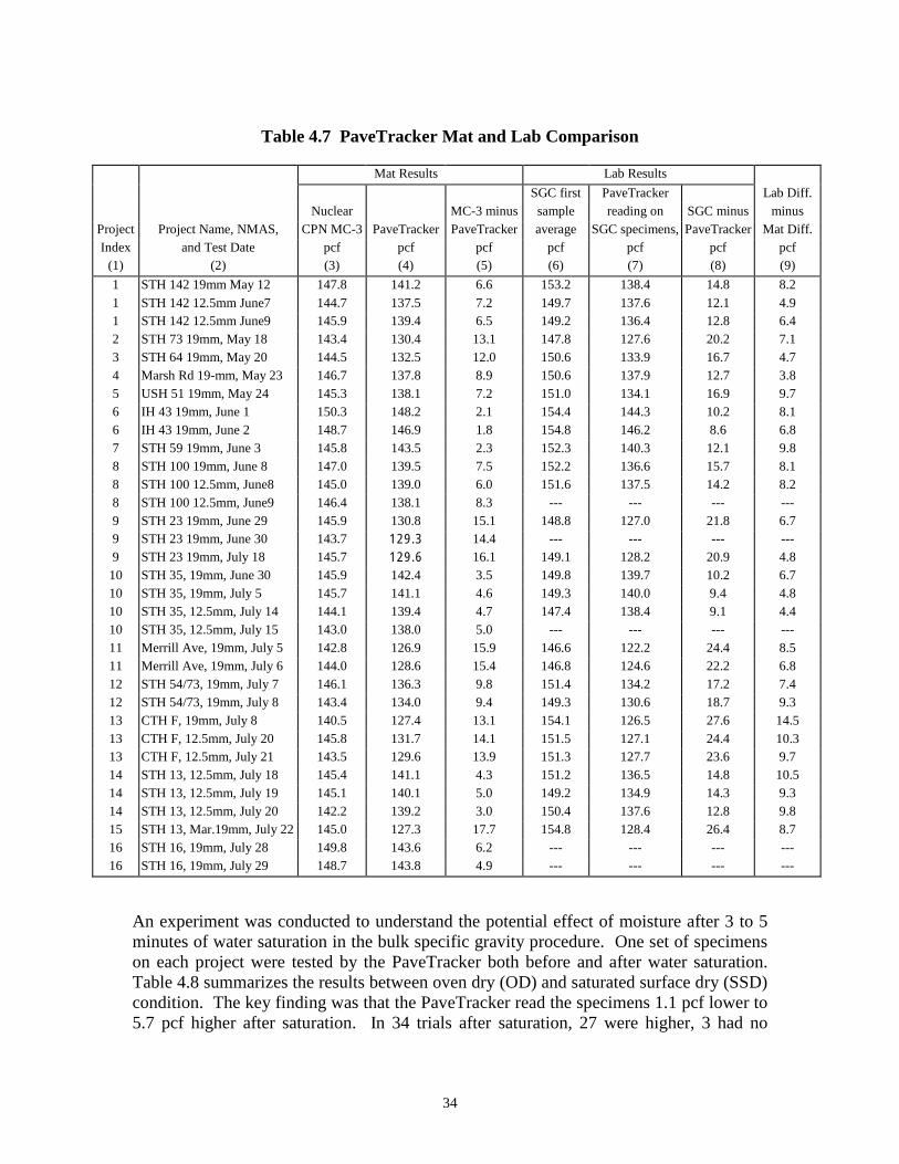
Table 4.7 PaveTracker Mat and Lab Comparison
Mat Results Lab Results
Lab Diff. SGC first PaveTracker Nuclear MC-3 minus sample reading on SGC minus minus
Project Project Name, NMAS, CPN MC-3 PaveTracker PaveTracker average SGC specimens, PaveTracker Mat Diff. Index and Test Date pcf pcf pcf pcf pcf pcf pcf
(1) (2) (3) (4) (5) (6) (7) (8) (9)
1 STH 142 19mm May 12 147.8 141.2 6.6 153.2 138.4 14.8 8.2 1 STH 142 12.5mm June7 144.7 137.5 7.2 149.7 137.6 12.1 4.9 1 STH 142 12.5mm June9 145.9 139.4 6.5 149.2 136.4 12.8 6.4 2 STH 73 19mm, May 18 143.4 130.4 13.1 147.8 127.6 20.2 7.1 3 STH 64 19mm, May 20 144.5 132.5 12.0 150.6 133.9 16.7 4.7 4 Marsh Rd 19-mm, May 23 146.7 137.8 8.9 150.6 137.9 12.7 3.8 5 USH 51 19mm, May 24 145.3 138.1 7.2 151.0 134.1 16.9 9.7 6 IH 43 19mm, June 1 150.3 148.2 2.1 154.4 144.3 10.2 8.1 6 IH 43 19mm, June 2 148.7 146.9 1.8 154.8 146.2 8.6 6.8 7 STH 59 19mm, June 3 145.8 143.5 2.3 152.3 140.3 12.1 9.8 8 STH 100 19mm, June 8 147.0 139.5 7.5 152.2 136.6 15.7 8.1 8 STH 100 12.5mm, June8 145.0 139.0 6.0 151.6 137.5 14.2 8.2 8 STH 100 12.5mm, June9 146.4 138.1 8.3 -- -- -- --9 STH 23 19mm, June 29 145.9 130.8 15.1 148.8 127.0 21.8 6.7 9 STH 23 19mm, June 30 143.7 129.3 14.4 -- -- -- --9 STH 23 19mm, July 18 145.7 129.6 16.1 149.1 128.2 20.9 4.8
10 STH 35, 19mm, June 30 145.9 142.4 3.5 149.8 139.7 10.2 6.7 10 STH 35, 19mm, July 5 145.7 141.1 4.6 149.3 140.0 9.4 4.8 10 STH 35, 12.5mm, July 14 144.1 139.4 4.7 147.4 138.4 9.1 4.4 10 STH 35, 12.5mm, July 15 143.0 138.0 5.0 -- -- -- --11 Merrill Ave, 19mm, July 5 142.8 126.9 15.9 146.6 122.2 24.4 8.5 11 Merrill Ave, 19mm, July 6 144.0 128.6 15.4 146.8 124.6 22.2 6.8 12 STH 54/73, 19mm, July 7 146.1 136.3 9.8 151.4 134.2 17.2 7.4 12 STH 54/73, 19mm, July 8 143.4 134.0 9.4 149.3 130.6 18.7 9.3 13 CTH F, 19mm, July 8 140.5 127.4 13.1 154.1 126.5 27.6 14.5 13 CTH F, 12.5mm, July 20 145.8 131.7 14.1 151.5 127.1 24.4 10.3 13 CTH F, 12.5mm, July 21 143.5 129.6 13.9 151.3 127.7 23.6 9.7 14 STH 13, 12.5mm, July 18 145.4 141.1 4.3 151.2 136.5 14.8 10.5 14 STH 13, 12.5mm, July 19 145.1 140.1 5.0 149.2 134.9 14.3 9.3 14 STH 13, 12.5mm, July 20 142.2 139.2 3.0 150.4 137.6 12.8 9.8 15 STH 13, Mar.19mm, July 22 145.0 127.3 17.7 154.8 128.4 26.4 8.7 16 STH 16, 19mm, July 28 149.8 143.6 6.2 -- -- -- --16 STH 16, 19mm, July 29 148.7 143.8 4.9 -- -- -- --
An experiment was conducted to understand the potential effect of moisture after 3 to 5 minutes of water saturation in the bulk specific gravity procedure. One set of specimens on each project were tested by the PaveTracker both before and after water saturation. Table 4.8 summarizes the results between oven dry (OD) and saturated surface dry (SSD) condition. The key finding was that the PaveTracker read the specimens 1.1 pcf lower to 5.7 pcf higher after saturation. In 34 trials after saturation, 27 were higher, 3 had no
34
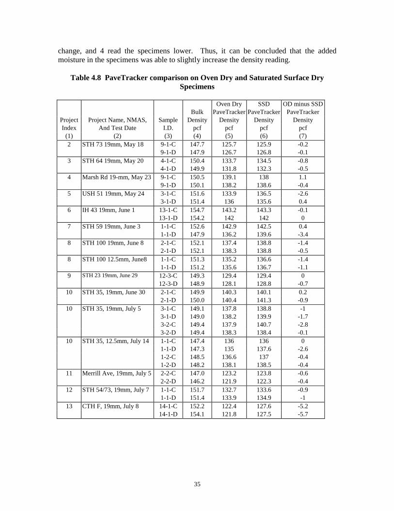
change, and 4 read the specimens lower. Thus, it can be concluded that the added moisture in the specimens was able to slightly increase the density reading.
Table 4.8 PaveTracker comparison on Oven Dry and Saturated Surface Dry Specimens
Oven Dry SSD OD minus SSD Bulk PaveTracker PaveTracker PaveTracker
Project Project Name, NMAS, Sample Density Density Density Density Index And Test Date I.D. pcf pcf pcf pcf
(1) (2) (3) (4) (5) (6) (7) 2 STH 73 19mm, May 18 9-1-C 147.7 125.7 125.9 -0.2
9-1-D 147.9 126.7 126.8 -0.1 3 STH 64 19mm, May 20 4-1-C 150.4 133.7 134.5 -0.8
4-1-D 149.9 131.8 132.3 -0.5 4 Marsh Rd 19-mm, May 23 9-1-C 150.5 139.1 138 1.1
9-1-D 150.1 138.2 138.6 -0.4 5 USH 51 19mm, May 24 3-1-C 151.6 133.9 136.5 -2.6
3-1-D 151.4 136 135.6 0.4 6 IH 43 19mm, June 1 13-1-C 154.7 143.2 143.3 -0.1
13-1-D 154.2 142 142 0 7 STH 59 19mm, June 3 1-1-C 152.6 142.9 142.5 0.4
1-1-D 147.9 136.2 139.6 -3.4 8 STH 100 19mm, June 8 2-1-C 152.1 137.4 138.8 -1.4
2-1-D 152.1 138.3 138.8 -0.5 8 STH 100 12.5mm, June8 1-1-C 151.3 135.2 136.6 -1.4
1-1-D 151.2 135.6 136.7 -1.1 9 STH 23 19mm, June 29 12-3-C 149.3 129.4 129.4 0
12-3-D 148.9 128.1 128.8 -0.7 10 STH 35, 19mm, June 30 2-1-C 149.9 140.3 140.1 0.2
2-1-D 150.0 140.4 141.3 -0.9 10 STH 35, 19mm, July 5 3-1-C
3-1-D 149.1 149.0
137.8 138.2
138.8 139.9
-1 -1.7
3-2-C 149.4 137.9 140.7 -2.8 3-2-D 149.4 138.3 138.4 -0.1
10 STH 35, 12.5mm, July 14 1-1-C 1-1-D
147.4 147.3
136 135
136 137.6
0 -2.6
1-2-C 148.5 136.6 137 -0.4 1-2-D 148.2 138.1 138.5 -0.4
11 Merrill Ave, 19mm, July 5 2-2-C 147.0 123.2 123.8 -0.6 2-2-D 146.2 121.9 122.3 -0.4
12 STH 54/73, 19mm, July 7 1-1-C 151.7 132.7 133.6 -0.9 1-1-D 151.4 133.9 134.9 -1
13 CTH F, 19mm, July 8 14-1-C 152.2 122.4 127.6 -5.2 14-1-D 154.1 121.8 127.5 -5.7
35
CHAPTER 5 ANALYSIS OF FACTORS
5.1 Introduction
This chapter investigated the affect of factors, or variables, on non-nuclear density readings. The previous chapter found that the average non-nuclear density readings fluctuated relative to the nuclear readings both between and within projects. The breakdown of the data into simple summary statistics did not have the capability to determine what factors impacted the readings. Therefore, a formal, statistically-valid determination was necessary.
5.2 Analysis of Variance
Analysis of variance (ANOVA) methods were used to determine which variables influenced changes in both nuclear and non-nuclear density readings, aside from changes in the actual pavement density itself. ANOVA can determine if the mean level within a specified feature of interest is different or not (i.e., aggregate source, NMAS, or any other meaningful feature). There are three fundamental types of ANOVA available, including the Fixed Effects Model (Model I ANOVA), the Random Effects Model (Model II ANOVA), and the Mixed Model, that uses a combination of fixed and random effects. For this study, the Random Effects Model was most appropriate since there were no specific treatments, or conditions, applied to any project variable. Adjustments in these variables were random in nature, and not specifically altered or adjusted to understand their effect. Three variables that were constant within a particular project mix, but varied between projects, included: (1) aggregate source (granite, gravel, and limestone), (2) NMAS (12.5mm or 19mm), and (3) ESALs in millions for a 20-year design life (0.3, 1, 3, 10, and 30).
A hypothesis test was used to determine if the mean level among any number of variables was significantly different or not. The null hypothesis, HO, hypothesized they were not different, while the alternative hypothesis, HA, hypothesized they were different:
HO: Features are not different (mean difference = 0). HA: Features are different (mean difference ≠ 0).
Two standard statistics were calculated and used to determine significance: (1) F-ratio and (2) p-value. The F-value calculated the ratio of mean variances “between” features and “within” features, and was then plotted on the F-distribution to determine a probability level of significance, or p-value. High F-ratios yielding p-values equal to or less than a traditional value of 5% would indicate the null hypothesis should be rejected. Equation 5.1 shows how the F-value is calculated using the mean squares (MS), or the average variance of “between” and “within” features:
36

MS (Between Feature) FFeature = .......…..(5.1)
MS (Within Feature)
The SAS statistical software package was used to perform the ANOVA calculations. The output provided two measures for the mean square - when the variable was entered first in the calculation (Type I), and when it was entered last (Type III). Type III provided the most rigorous hypothesis test since most of the variability has been assigned to the previously entered variables, and only the remaining unexplained variation was accounted for by the last variable. For that reason, Type III Sum of Squares, and resulting Mean Squares, was used in the F-ratio calculation. Then, p-values were assigned to the F-ratio based on the sample size and degrees of freedom, or pieces of data used in determination minus one for the mean itself. Traditionally, a 0.05 cutoff value would be used to determine significance. However, in this analysis, four probability ranges were reported to assess the relative degree of significance, including: (1) less than 0.01, (2) between 0.01 and 0.05, (3) between 0.05 and 0.1, and (4) greater than 0.1.
5.3 Results of ANOVA for All Project Gauges
Table 5.1 provides the ANOVA results for each variable in explaining variation in mean nuclear and non-nuclear density readings, except for the actual change in density of the pavement itself. The table provides the variable, sample size, degrees of freedom, and p-value range. The maximum number of test sites in the study was 876, tested by both the project nuclear gauge (CPN MC3) and PaveTracker, as shown in Columns 3 and 5. In Columns 4 and 6, each gauge included the PQI moisture and temperature readings in the analysis, and the number of test sites was reduced to 546. This reduction was the result of not having the PQI 300 and PQI 301 operating on all 16 projects. The PQI 300 and PQI 301 gauges tested 693 and 722 test sites, respectively, and 546 test sites mutually.
Results for the MC3 and PaveTracker gauges, both with and without the temperature and moisture readings, were inconsistent, indicating the instability of testing the variables on different projects. The following sections analyzed the significant variables.
37
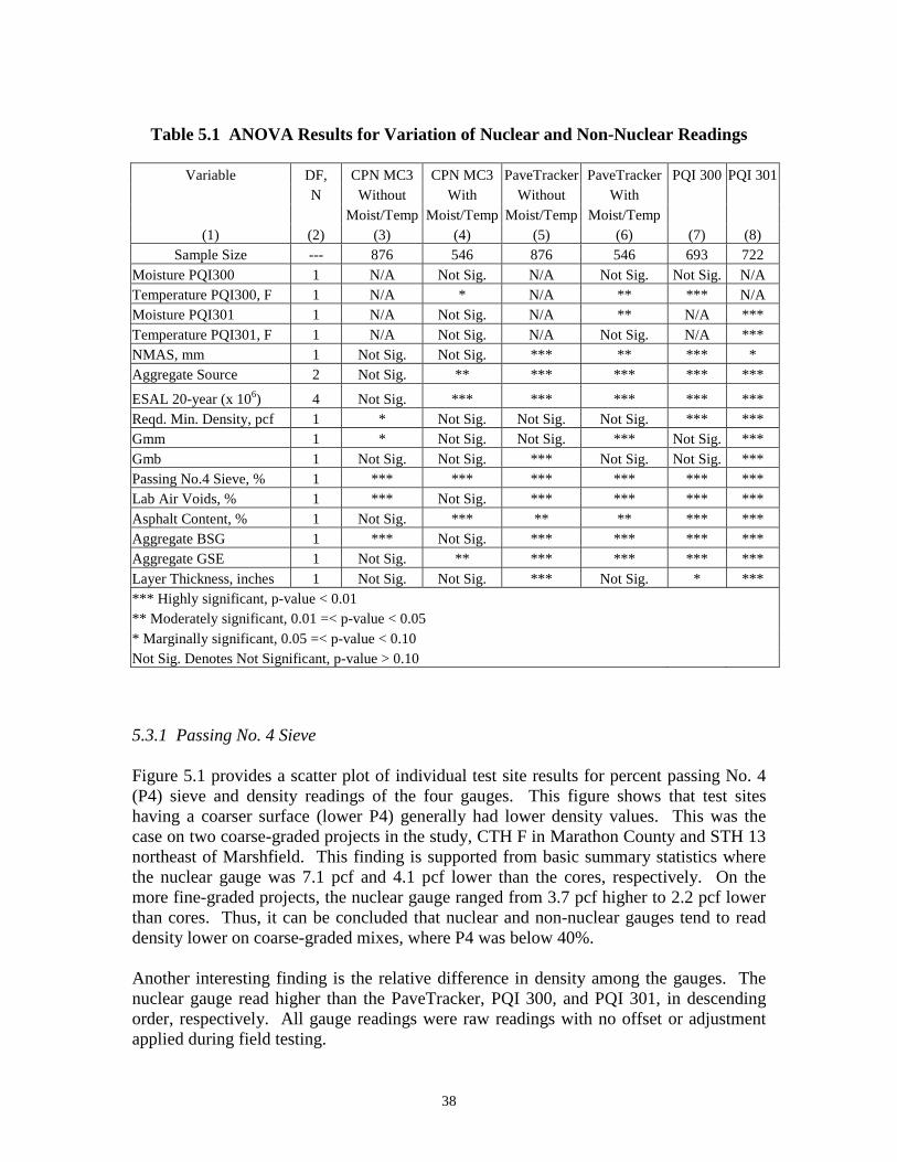
Table 5.1 ANOVA Results for Variation of Nuclear and Non-Nuclear Readings
Variable
(1)
DF, N
(2)
CPN MC3 Without
Moist/Temp (3)
CPN MC3 With
Moist/Temp (4)
PaveTracker Without
Moist/Temp (5)
PaveTracker With
Moist/Temp (6)
PQI 300
(7)
PQI 301
(8) Sample Size -- 876 546 876 546 693 722
Moisture PQI300 1 N/A Not Sig. N/A Not Sig. Not Sig. N/A Temperature PQI300, F 1 N/A * N/A ** *** N/A Moisture PQI301 1 N/A Not Sig. N/A ** N/A *** Temperature PQI301, F 1 N/A Not Sig. N/A Not Sig. N/A *** NMAS, mm 1 Not Sig. Not Sig. *** ** *** * Aggregate Source 2 Not Sig. ** *** *** *** ***
ESAL 20-year (x 106) 4 Not Sig. *** *** *** *** *** Reqd. Min. Density, pcf 1 * Not Sig. Not Sig. Not Sig. *** *** Gmm 1 * Not Sig. Not Sig. *** Not Sig. *** Gmb 1 Not Sig. Not Sig. *** Not Sig. Not Sig. *** Passing No.4 Sieve, % 1 *** *** *** *** *** *** Lab Air Voids, % 1 *** Not Sig. *** *** *** *** Asphalt Content, % 1 Not Sig. *** ** ** *** *** Aggregate BSG 1 *** Not Sig. *** *** *** *** Aggregate GSE 1 Not Sig. ** *** *** *** *** Layer Thickness, inches 1 Not Sig. Not Sig. *** Not Sig. * *** *** Highly significant, p-value < 0.01 ** Moderately significant, 0.01 =< p-value < 0.05 * Marginally significant, 0.05 =< p-value < 0.10 Not Sig. Denotes Not Significant, p-value > 0.10
5.3.1 Passing No. 4 Sieve
Figure 5.1 provides a scatter plot of individual test site results for percent passing No. 4 (P4) sieve and density readings of the four gauges. This figure shows that test sites having a coarser surface (lower P4) generally had lower density values. This was the case on two coarse-graded projects in the study, CTH F in Marathon County and STH 13 northeast of Marshfield. This finding is supported from basic summary statistics where the nuclear gauge was 7.1 pcf and 4.1 pcf lower than the cores, respectively. On the more fine-graded projects, the nuclear gauge ranged from 3.7 pcf higher to 2.2 pcf lower than cores. Thus, it can be concluded that nuclear and non-nuclear gauges tend to read density lower on coarse-graded mixes, where P4 was below 40%.
Another interesting finding is the relative difference in density among the gauges. The nuclear gauge read higher than the PaveTracker, PQI 300, and PQI 301, in descending order, respectively. All gauge readings were raw readings with no offset or adjustment applied during field testing.
38
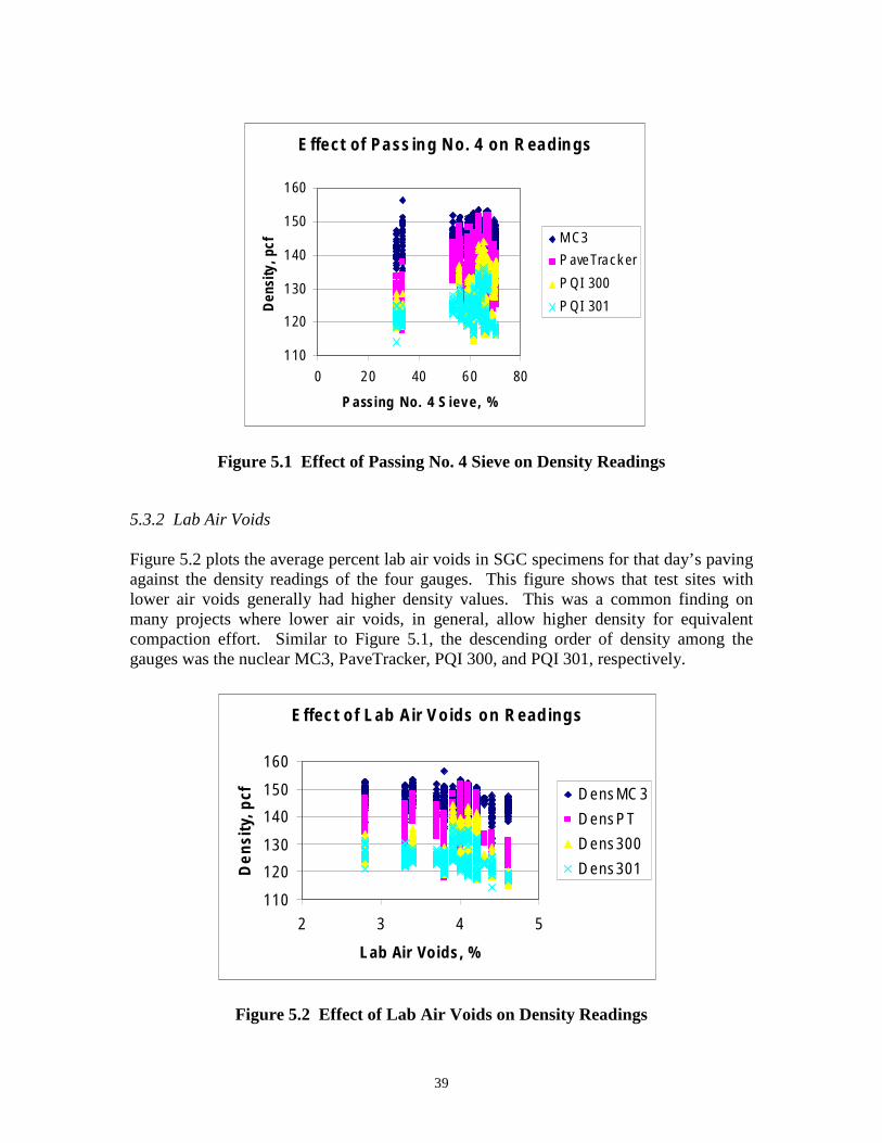
Effect of Passing No. 4 on Readings
160
150
Den
sity
, pcf
140 MC3
PaveTracker
120
130 PQI 300
PQI 301
110
0 20 40 60 80
Passing No. 4 Sieve, %
Figure 5.1 Effect of Passing No. 4 Sieve on Density Readings
5.3.2 Lab Air Voids Figure 5.2 plots the average percent lab air voids in SGC specimens for that day’s paving against the density readings of the four gauges. This figure shows that test sites with lower air voids generally had higher density values. This was a common finding on many projects where lower air voids, in general, allow higher density for equivalent compaction effort. Similar to Figure 5.1, the descending order of density among the gauges was the nuclear MC3, PaveTracker, PQI 300, and PQI 301, respectively.
Effect of Lab Air Voids on Readings
160
De
nsi
ty, p
cf 150 DensMC3 140
DensPT
130 Dens300
120 Dens301
110
2 3 4 5
Lab Air Voids, %
Figure 5.2 Effect of Lab Air Voids on Density Readings
39
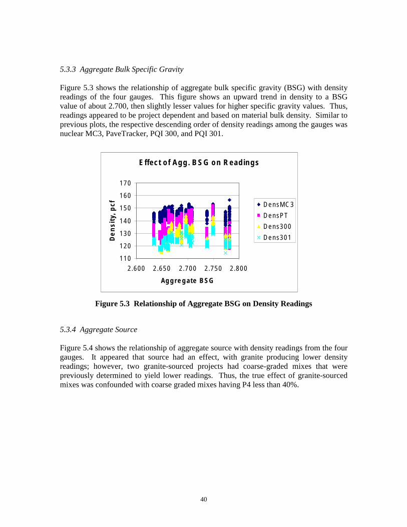
5.3.3 Aggregate Bulk Specific Gravity Figure 5.3 shows the relationship of aggregate bulk specific gravity (BSG) with density readings of the four gauges. This figure shows an upward trend in density to a BSG value of about 2.700, then slightly lesser values for higher specific gravity values. Thus, readings appeared to be project dependent and based on material bulk density. Similar to previous plots, the respective descending order of density readings among the gauges was nuclear MC3, PaveTracker, PQI 300, and PQI 301.
Effect of Agg. BSG on Readings
170
160
150
140
130 120 110 2.600
De
nsi
ty, p
cf
DensMC3
DensPT Dens300 Dens301
2.650 2.700 2.750 2.800
Aggregate BSG
Figure 5.3 Relationship of Aggregate BSG on Density Readings 5.3.4 Aggregate Source Figure 5.4 shows the relationship of aggregate source with density readings from the four gauges. It appeared that source had an effect, with granite producing lower density readings; however, two granite-sourced projects had coarse-graded mixes that were previously determined to yield lower readings. Thus, the true effect of granite-sourced mixes was confounded with coarse graded mixes having P4 less than 40%.
40
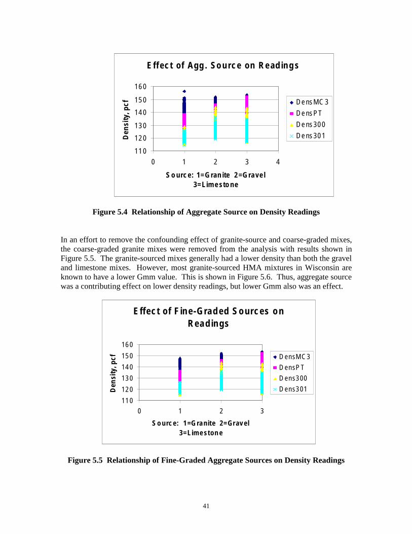
Effect of Agg. Source on Readings
160
Den
sity
, pcf 150 DensMC3
140 DensPT
130 Dens300
120 Dens301
110 0 1 2 3 4
Source: 1=Granite 2=Gravel 3=Limestone
Figure 5.4 Relationship of Aggregate Source on Density Readings
In an effort to remove the confounding effect of granite-source and coarse-graded mixes, the coarse-graded granite mixes were removed from the analysis with results shown in Figure 5.5. The granite-sourced mixes generally had a lower density than both the gravel and limestone mixes. However, most granite-sourced HMA mixtures in Wisconsin are known to have a lower Gmm value. This is shown in Figure 5.6. Thus, aggregate source was a contributing effect on lower density readings, but lower Gmm also was an effect.
Effect of Fine-Graded Sources on
Readings
160
Den
sity
, pcf 150 DensMC3
140 DensPT
130 Dens300
120 Dens301
110 0 1 2 3
Source: 1=Granite 2=Gravel 3=Limestone
Figure 5.5 Relationship of Fine-Graded Aggregate Sources on Density Readings
41
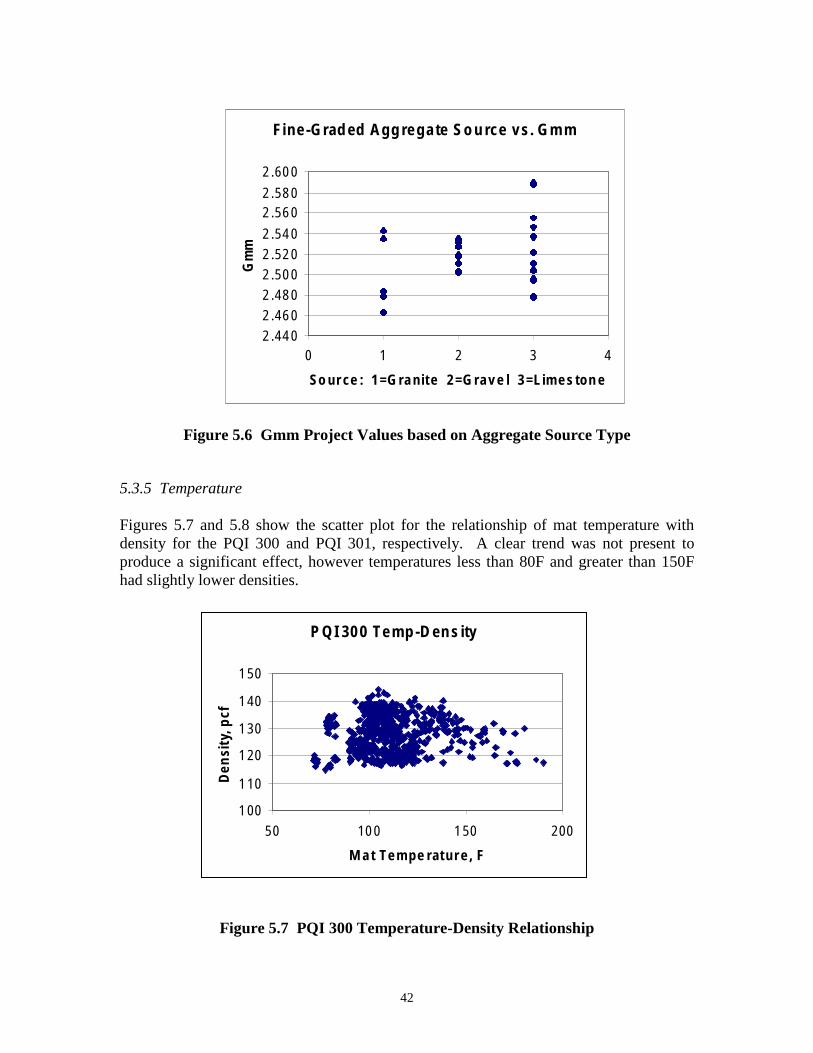
Gm
m
Fine-Graded Aggregate Source vs. Gmm
2.600
2.580 2.560
2.540 2.520 2.500 2.480 2.460 2.440
0 1 2 3 4
Source: 1=Granite 2=Gravel 3=Limestone
Figure 5.6 Gmm Project Values based on Aggregate Source Type
5.3.5 Temperature
Figures 5.7 and 5.8 show the scatter plot for the relationship of mat temperature with density for the PQI 300 and PQI 301, respectively. A clear trend was not present to produce a significant effect, however temperatures less than 80F and greater than 150F had slightly lower densities.
PQI 300 Temp-Density
150
140
Den
sity
, pcf
130
120
110
100 50 100 150
Mat Temperature, F
200
Figure 5.7 PQI 300 Temperature-Density Relationship
42
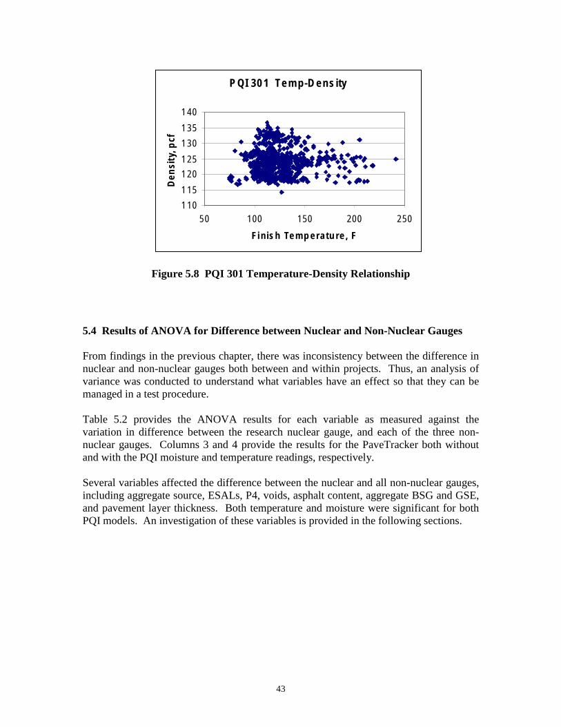
D
ensi
ty, p
cf
PQI 301 Temp-Density
140
135
130
125
120
115
110 50 100 150 200 250
Finish Temperature, F
Figure 5.8 PQI 301 Temperature-Density Relationship
5.4 Results of ANOVA for Difference between Nuclear and Non-Nuclear Gauges
From findings in the previous chapter, there was inconsistency between the difference in nuclear and non-nuclear gauges both between and within projects. Thus, an analysis of variance was conducted to understand what variables have an effect so that they can be managed in a test procedure.
Table 5.2 provides the ANOVA results for each variable as measured against the variation in difference between the research nuclear gauge, and each of the three nonnuclear gauges. Columns 3 and 4 provide the results for the PaveTracker both without and with the PQI moisture and temperature readings, respectively.
Several variables affected the difference between the nuclear and all non-nuclear gauges, including aggregate source, ESALs, P4, voids, asphalt content, aggregate BSG and GSE, and pavement layer thickness. Both temperature and moisture were significant for both PQI models. An investigation of these variables is provided in the following sections.
43
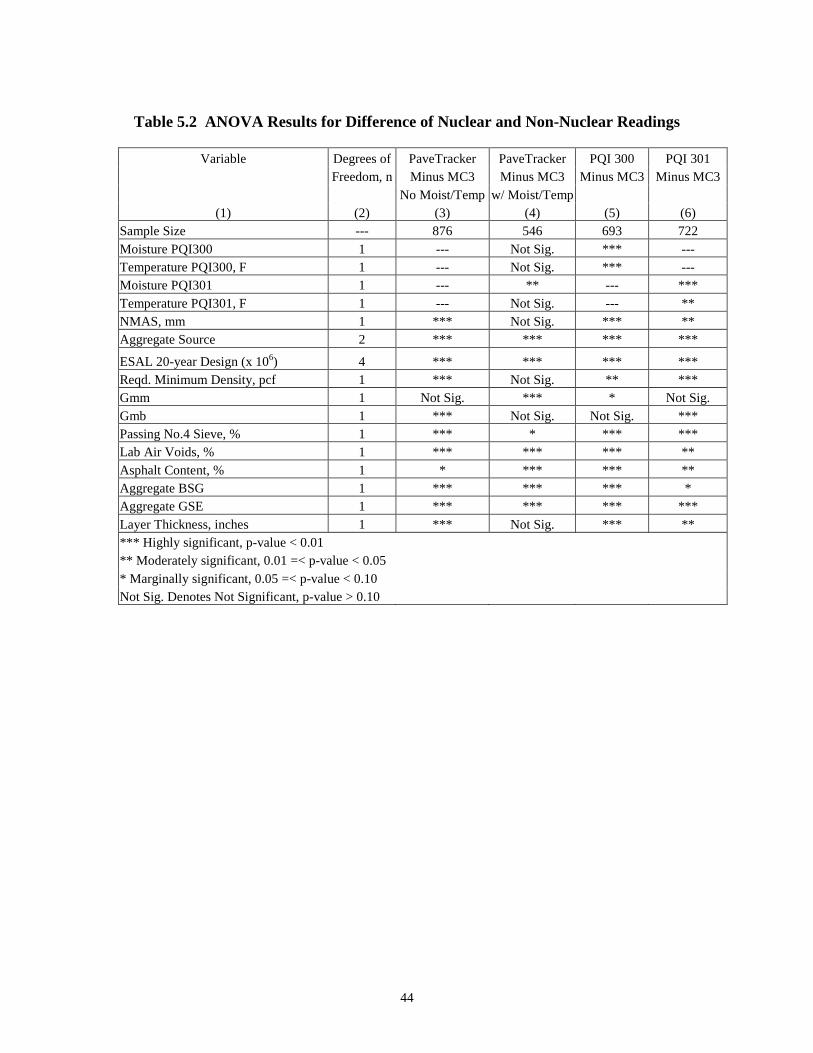
Table 5.2 ANOVA Results for Difference of Nuclear and Non-Nuclear Readings
Variable
(1)
Degrees of Freedom, n
(2)
PaveTracker Minus MC3
No Moist/Temp (3)
PaveTracker Minus MC3
w/ Moist/Temp (4)
PQI 300 Minus MC3
(5)
PQI 301 Minus MC3
(6) Sample Size -- 876 546 693 722 Moisture PQI300 1 -- Not Sig. *** --Temperature PQI300, F 1 -- Not Sig. *** --Moisture PQI301 1 -- ** -- *** Temperature PQI301, F 1 -- Not Sig. -- ** NMAS, mm 1 *** Not Sig. *** ** Aggregate Source 2 *** *** *** ***
ESAL 20-year Design (x 106) 4 *** *** *** *** Reqd. Minimum Density, pcf 1 *** Not Sig. ** *** Gmm 1 Not Sig. *** * Not Sig. Gmb 1 *** Not Sig. Not Sig. *** Passing No.4 Sieve, % 1 *** * *** *** Lab Air Voids, % 1 *** *** *** ** Asphalt Content, % 1 * *** *** ** Aggregate BSG 1 *** *** *** * Aggregate GSE 1 *** *** *** *** Layer Thickness, inches 1 *** Not Sig. *** ** *** Highly significant, p-value < 0.01 ** Moderately significant, 0.01 =< p-value < 0.05 * Marginally significant, 0.05 =< p-value < 0.10 Not Sig. Denotes Not Significant, p-value > 0.10
44
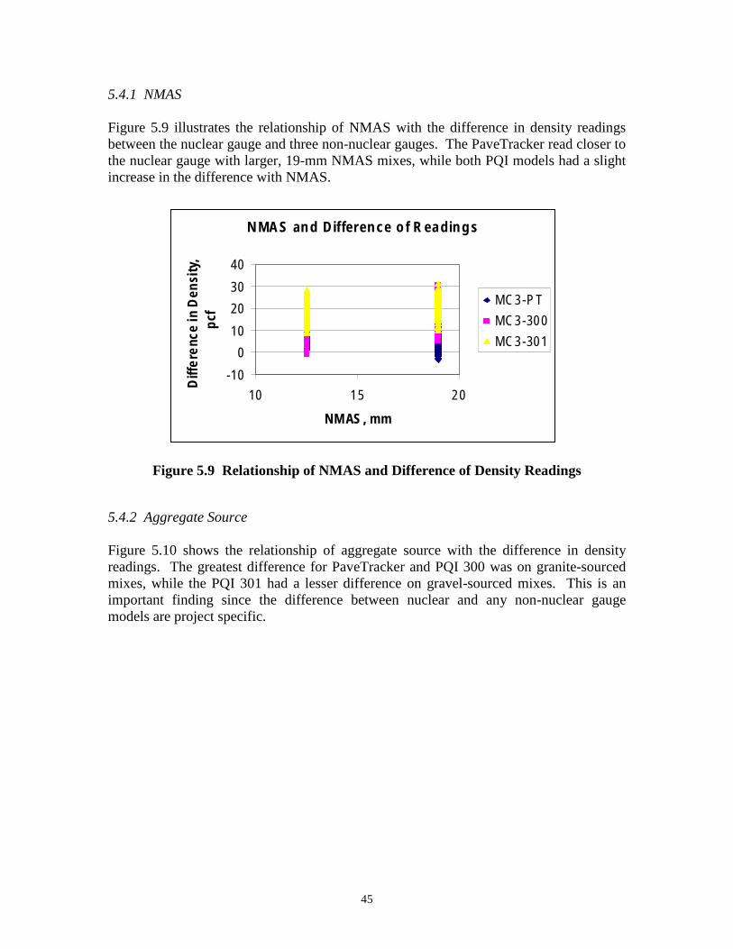
5.4.1 NMAS Figure 5.9 illustrates the relationship of NMAS with the difference in density readings between the nuclear gauge and three non-nuclear gauges. The PaveTracker read closer to the nuclear gauge with larger, 19-mm NMAS mixes, while both PQI models had a slight increase in the difference with NMAS.
NMAS and Difference of Readings
40 ity,
30 ns
20
pcf n D
e MC3-PT
MC3-300 10
Diff
eren
ce i
MC3-301 0
-10
10 15 20
NMAS, mm
Figure 5.9 Relationship of NMAS and Difference of Density Readings
5.4.2 Aggregate Source Figure 5.10 shows the relationship of aggregate source with the difference in density readings. The greatest difference for PaveTracker and PQI 300 was on granite-sourced mixes, while the PQI 301 had a lesser difference on gravel-sourced mixes. This is an important finding since the difference between nuclear and any non-nuclear gauge models are project specific.
45
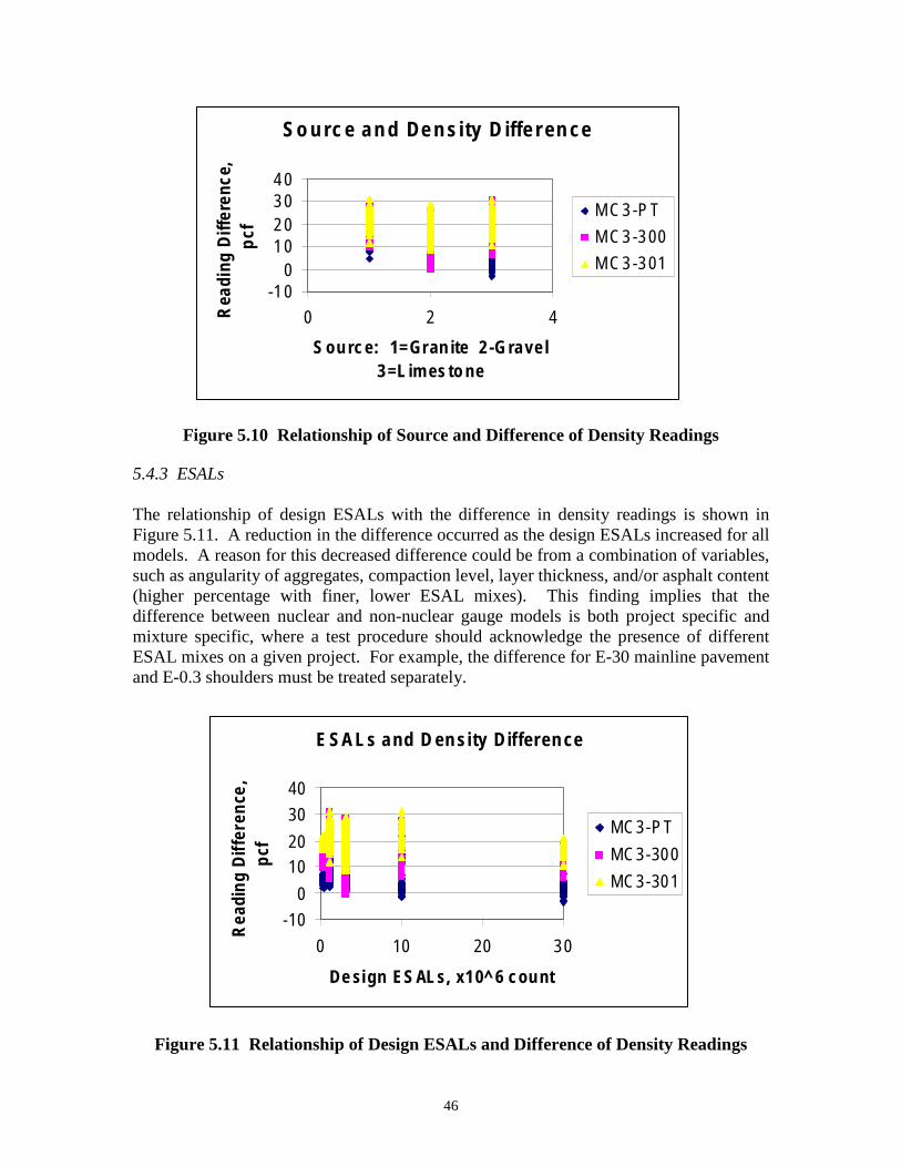
Source and Density Difference
Rea
ding
Diff
eren
ce,
pcf
40 30 20 10
0 -10
0 2 4
Source: 1=Granite 2-Gravel 3=Limestone
MC3-PT
MC3-300
MC3-301
Figure 5.10 Relationship of Source and Difference of Density Readings
5.4.3 ESALs The relationship of design ESALs with the difference in density readings is shown in Figure 5.11. A reduction in the difference occurred as the design ESALs increased for all models. A reason for this decreased difference could be from a combination of variables, such as angularity of aggregates, compaction level, layer thickness, and/or asphalt content (higher percentage with finer, lower ESAL mixes). This finding implies that the difference between nuclear and non-nuclear gauge models is both project specific and mixture specific, where a test procedure should acknowledge the presence of different ESAL mixes on a given project. For example, the difference for E-30 mainline pavement and E-0.3 shoulders must be treated separately.
ESALs and Density Difference
Rea
ding
Diff
eren
ce,
pcf
-10
0
10 20
30
40
0 10 20 30
MC3-PT
MC3-300
MC3-301
Design ESALs, x10^6 count
Figure 5.11 Relationship of Design ESALs and Difference of Density Readings
46
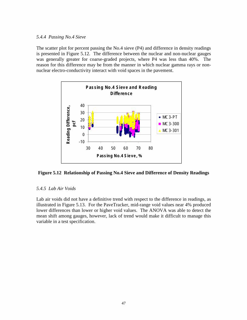
5.4.4 Passing No.4 Sieve The scatter plot for percent passing the No.4 sieve (P4) and difference in density readings is presented in Figure 5.12. The difference between the nuclear and non-nuclear gauges was generally greater for coarse-graded projects, where P4 was less than 40%. The reason for this difference may be from the manner in which nuclear gamma rays or nonnuclear electro-conductivity interact with void spaces in the pavement.
Passing No.4 Sieve and Reading
Difference
40 e,
30 enc
20
pcf
MC3-PT
Rea
ding
Diff
er
MC3-300 10
MC3-301 0
-10
30 40 50 60 70 80
Passing No.4 Sieve, %
Figure 5.12 Relationship of Passing No.4 Sieve and Difference of Density Readings
5.4.5 Lab Air Voids Lab air voids did not have a definitive trend with respect to the difference in readings, as illustrated in Figure 5.13. For the PaveTracker, mid-range void values near 4% produced lower differences than lower or higher void values. The ANOVA was able to detect the mean shift among gauges, however, lack of trend would make it difficult to manage this variable in a test specification.
47
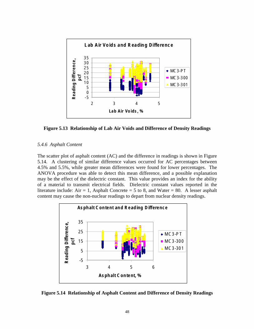
Lab Air Voids and Reading Difference
Rea
din
g D
iffer
ence
, p
cf
35 30
20 25
MC3-PT
15 MC3-300
5 10 MC3-301
0 -5
2 3 4 5
Lab Air Voids, %
Figure 5.13 Relationship of Lab Air Voids and Difference of Density Readings
5.4.6 Asphalt Content The scatter plot of asphalt content (AC) and the difference in readings is shown in Figure 5.14. A clustering of similar difference values occurred for AC percentages between 4.5% and 5.5%, while greater mean differences were found for lower percentages. The ANOVA procedure was able to detect this mean difference, and a possible explanation may be the effect of the dielectric constant. This value provides an index for the ability of a material to transmit electrical fields. Dielectric constant values reported in the literature include: Air = 1, Asphalt Concrete = 5 to 8, and Water = 80. A lesser asphalt content may cause the non-nuclear readings to depart from nuclear density readings.
Asphalt Content and Reading Difference
Rea
ding
Diff
eren
ce,
pcf
35
25 MC3-PT
15 MC3-300
5 MC3-301
-5 3 4 5 6
Asphalt Content, %
Figure 5.14 Relationship of Asphalt Content and Difference of Density Readings
48
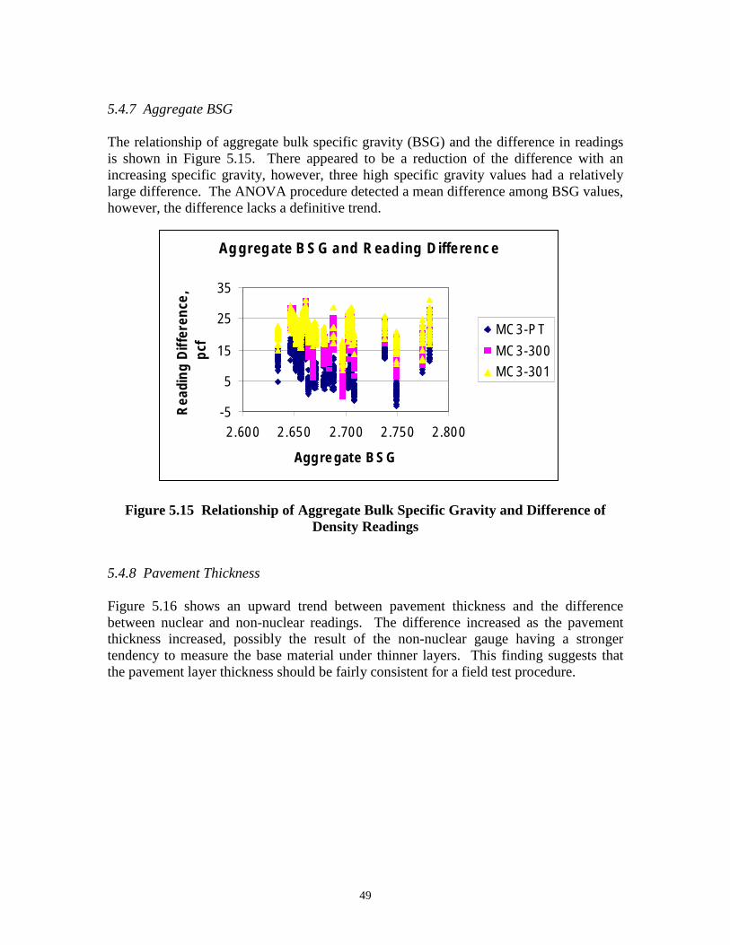
Rea
ding
Diff
eren
ce,
pcf
5.4.7 Aggregate BSG The relationship of aggregate bulk specific gravity (BSG) and the difference in readings is shown in Figure 5.15. There appeared to be a reduction of the difference with an increasing specific gravity, however, three high specific gravity values had a relatively large difference. The ANOVA procedure detected a mean difference among BSG values, however, the difference lacks a definitive trend.
Aggregate BSG and Reading Difference
35
25 MC3-PT
15 MC3-300
MC3-301 5
-5 2.600 2.650 2.700 2.750 2.800
Aggregate BSG
Figure 5.15 Relationship of Aggregate Bulk Specific Gravity and Difference of
Density Readings 5.4.8 Pavement Thickness Figure 5.16 shows an upward trend between pavement thickness and the difference between nuclear and non-nuclear readings. The difference increased as the pavement thickness increased, possibly the result of the non-nuclear gauge having a stronger tendency to measure the base material under thinner layers. This finding suggests that the pavement layer thickness should be fairly consistent for a field test procedure.
49

Pavement Thickness and Reading
Difference
Diff
ere
nce,
pcf
35 R
eadi
ng 25 MC3-PT
15 MC3-300
5 MC3-301
-5
1 2 3 4
Pavement Thickness, inches
Figure 5.16 Relationship of Pavement Thickness and Difference of Density
Readings 5.4.9 Temperature Figures 5.17 and 5.18 show the relationship of mat temperature with density difference for the PQI 300 and PQI 301, respectively. For the PQI 300, as temperatures increased from 120 to 180F, there was an increase in the difference, however, a cluster with no trend was observed below 120F. This suggests that non-nuclear QC testing behind the breakdown roller with the PQI 300 may yield a greater difference with a baseline nuclear reading, than testing behind the cold roller. However, no visible trend was observed with the PQI 300.
50
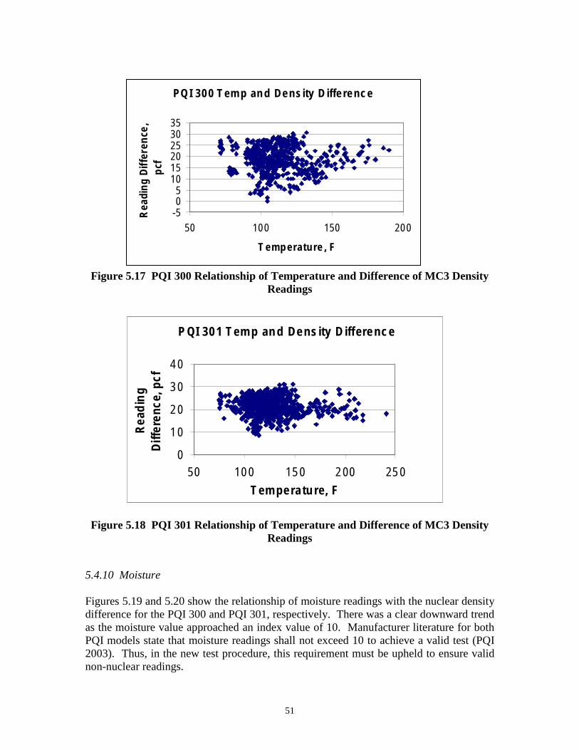
R
eadi
ng D
iffer
ence
,pc
f
PQI 300 Temp and Density Difference
35 30 25 20 15 10 5 0
-5 50 100 150 200
Temperature, F
Figure 5.17 PQI 300 Relationship of Temperature and Difference of MC3 Density Readings
PQI 301 Temp and Density Difference
40
Rea
din
gD
iffer
ence
, pcf
30
20
10
0 50 100 150 200 250
Temperature, F
Figure 5.18 PQI 301 Relationship of Temperature and Difference of MC3 Density Readings
5.4.10 Moisture
Figures 5.19 and 5.20 show the relationship of moisture readings with the nuclear density difference for the PQI 300 and PQI 301, respectively. There was a clear downward trend as the moisture value approached an index value of 10. Manufacturer literature for both PQI models state that moisture readings shall not exceed 10 to achieve a valid test (PQI 2003). Thus, in the new test procedure, this requirement must be upheld to ensure valid non-nuclear readings.
51
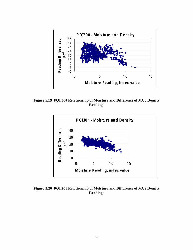
Rea
din
g D
iffer
ence
,p
cf
PQI300 - Moisture and Density 35 30 25 20 15 10
5 0
-5 0 5 10 15
Moisture Reading, index value
Figure 5.19 PQI 300 Relationship of Moisture and Difference of MC3 Density Readings
PQI301 - Moisture and Density
Rea
ding
Diff
eren
ce,
pcf
40
30
20
10
0 0 5 10 15
Moisture Reading, index value
Figure 5.20 PQI 301 Relationship of Moisture and Difference of MC3 Density Readings
52
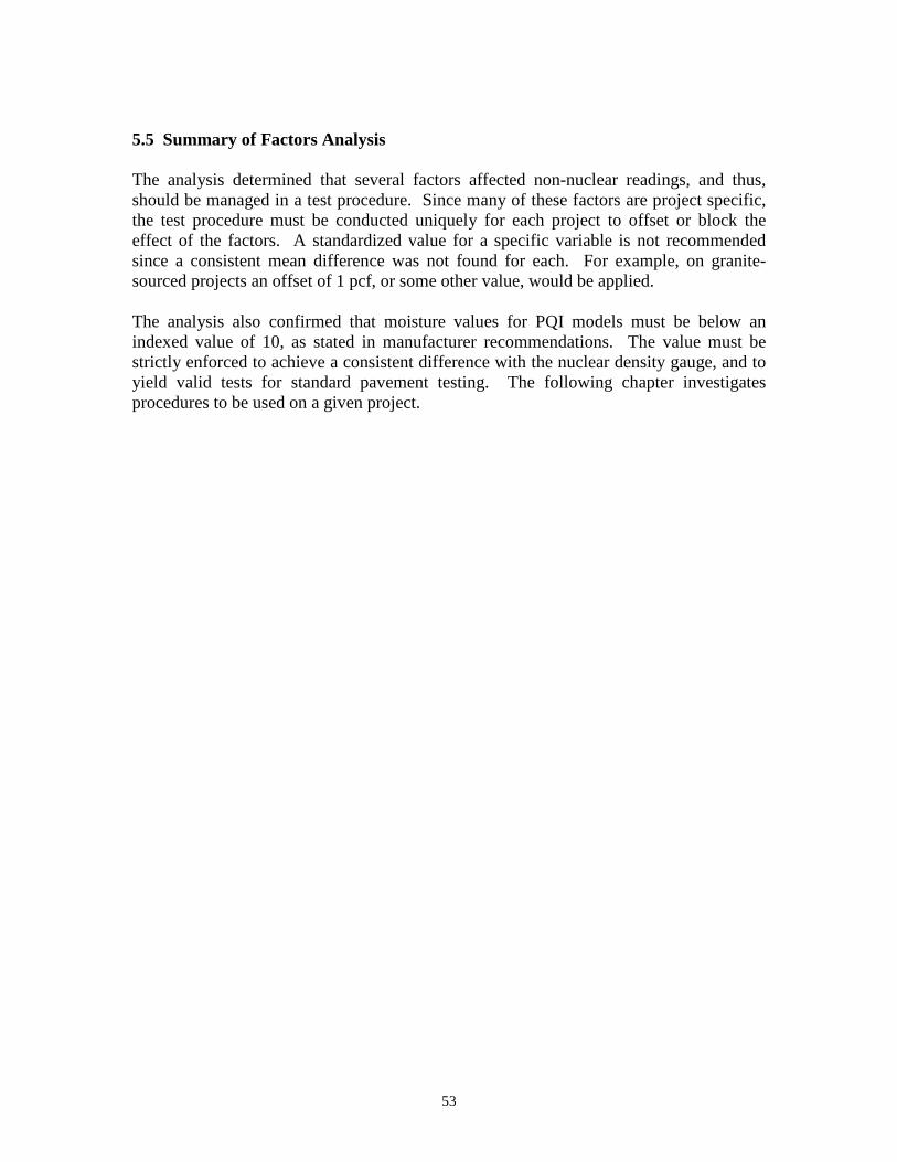
5.5 Summary of Factors Analysis
The analysis determined that several factors affected non-nuclear readings, and thus, should be managed in a test procedure. Since many of these factors are project specific, the test procedure must be conducted uniquely for each project to offset or block the effect of the factors. A standardized value for a specific variable is not recommended since a consistent mean difference was not found for each. For example, on granite-sourced projects an offset of 1 pcf, or some other value, would be applied.
The analysis also confirmed that moisture values for PQI models must be below an indexed value of 10, as stated in manufacturer recommendations. The value must be strictly enforced to achieve a consistent difference with the nuclear density gauge, and to yield valid tests for standard pavement testing. The following chapter investigates procedures to be used on a given project.
53

CHAPTER 6 INVESTIGATION OF CALIBRATION PROCEDURES
6.1 Introduction
The previous chapters determined that a project-specific test procedure is necessary to calibrate the non-nuclear gauge for a given project. In this chapter, several calibration procedures are first proposed, then an analysis investigates the most effective methods for a test specification.
6.2 Calibration Procedures
Potential calibration procedures and preliminary considerations and recommendations are enumerated in Table 6.1.
Table 6.1 Potential Calibration Procedures
Index (1)
Procedure (2)
Considerations and Recommendation (3)
1 Do Nothing. Use Non-nuclear gauge directly after start-up.
• Mean difference between non-nuclear and non-nuclear gauge varies between and within projects.
• Non-nuclear gauge generally reads lower than nuclear gauge from 1 to 27 pcf.
• Procedure not recommended. 2 Test Blocks • Non-nuclear readings were scattered and inaccurately
measured test block density. • Truax Lab - PQI Model #301 readings ranged from 37.9
pcf below to 16.8 pcf above to the known block density. • Truax Lab - PaveTracker readings ranged from 28.6 pcf
above to 22.8 pcf below. • Procedure not recommended.
3 Manufacturer Reference Block
• Only available with PaveTracker model. • Although the PaveTracker model was able to measure
the manufacturer reference block within ± 0.2 pcf after a half day of testing, it was unable to calibrate an offset to the specific mat.
• Procedure not recommended. 4 Superpave Gyratory
Compactor (SGC) Specimens
• Only available with PaveTracker model. • PaveTracker read the SGC specimens from 3.8 to
10.5pcf lower than the nuclear density gauge offset for the same project and mix type.
• Lab-compacted specimens do not provide a reliable offset value for use on the mat.
• Procedure not recommended. 5 Nuclear Density
Gauge • Mean difference varies between and within projects. • Investigation of procedure recommended.
54
From this table, investigation of only one calibration procedure is recommended – calibration to the nuclear density gauge. The other procedures, including “do nothing”, test blocks (Truax Lab or District Lab), manufacturer reference block, and Superpave gyratory specimens, do not have the capability to provide a reliable calibration offset. Prior data analysis support this conclusion. Thus, in the following sections, the calibration procedure using the nuclear density gauge is investigated.
6.3 Development of Calibration Procedures
The goal in development of the calibration procedure was to compare the non-nuclear density reading from each device against the corresponding nuclear density readings, then estimate the error magnitudes and develop correlations for each device. The correlations developed will essentially form the adjustment factors required to determine in-situ density comparable to the nuclear gauge readings within a tolerable accuracy level.
Previous tables in the report have grouped data by projects. However, for the purpose of analyzing mean densities and variations, the data were split by mix design and each day of paving. Table 6.2 presents the calculated mean and standard deviation of the densities measured with the nuclear and non-nuclear gauges for each project. Each mix identification (ID) in Table 6.2 refers to a unique combination of highway number, NMAS, aggregate source, and HMA layer. Note that these results refer to the data from the overall project, but are grouped by each day of testing to reflect changes in density values and resulting standard deviation with each day of paving. Further, the data from roller compaction sites are grouped separately for each project. The number of test points included in the computation of the average and standard deviation values is tabulated along with other project details such as route number, test date, NMAS and aggregate type. It is of interest to note from the data presented in Table 6.2, that in more than 81 percent of the test sites, and in 77 percent of the roller compaction test sites, the standard deviation in the density measurements are higher for the nuclear gauge than for the nonnuclear gauges.
During the data collection process, testing at each test site within a project included 1 nuclear gauge reading and 5 non-nuclear gauge readings (clustered testing). The standard deviation of the 5 readings at each test point was calculated to assess the repeatability of measurements using the non-nuclear gauge. The mean of the standard deviation at each test point for each mix ID is reported in Table 6.3, along with the overall mix ID standard deviation from the nuclear gauge readings. Figure 6.1 provides a graphical illustration of this data.
55
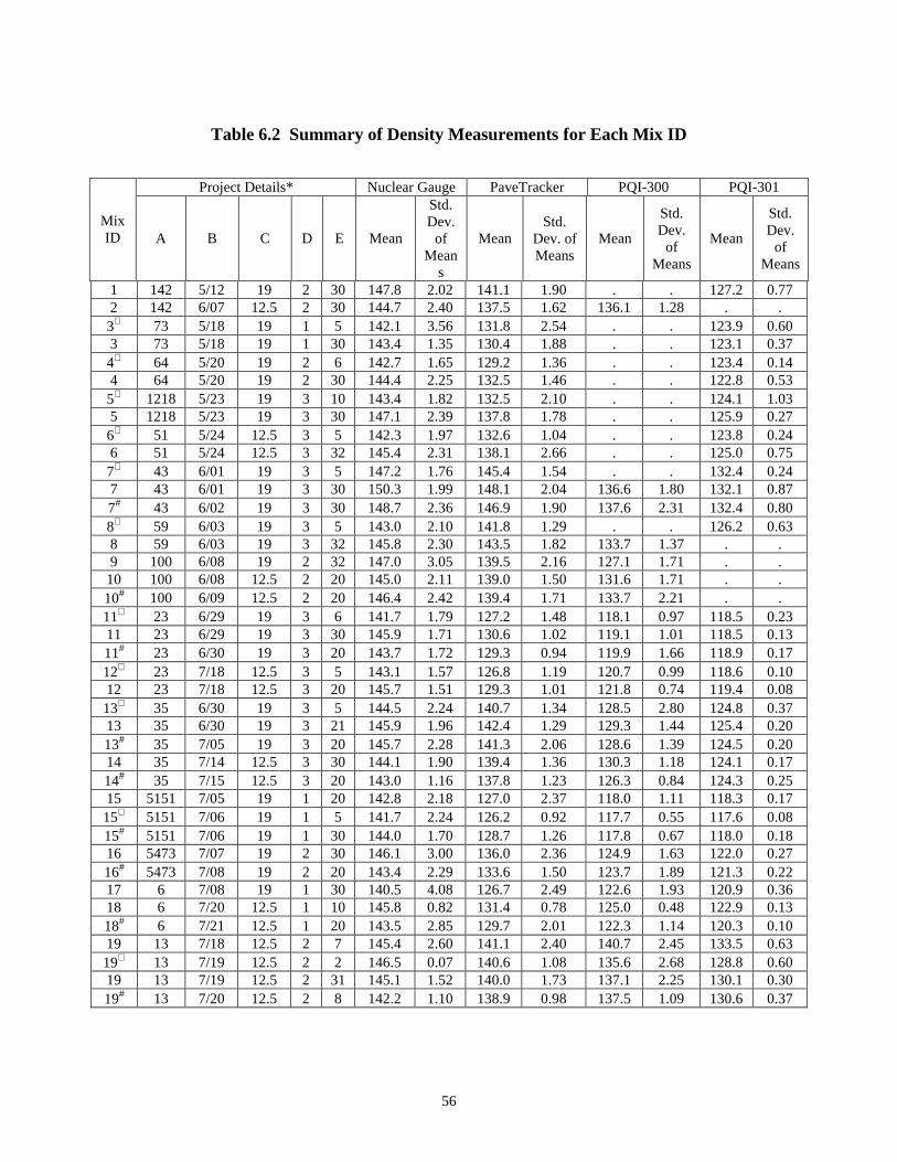
Table 6.2 Summary of Density Measurements for Each Mix ID
Mix ID
Project Details* Nuclear Gauge PaveTracker PQI-300 PQI-301
A B C D E Mean
Std. Dev.
of Mean
s
Mean Std.
Dev. of Means
Mean
Std. Dev.
of Means
Mean
Std. Dev.
of Means
1 142 5/12 19 2 30 147.8 2.02 141.1 1.90 . . 127.2 0.77 2 142 6/07 12.5 2 30 144.7 2.40 137.5 1.62 136.1 1.28 . . 3⊗ 73 5/18 19 1 5 142.1 3.56 131.8 2.54 . . 123.9 0.60 3 73 5/18 19 1 30 143.4 1.35 130.4 1.88 . . 123.1 0.37 4⊗ 64 5/20 19 2 6 142.7 1.65 129.2 1.36 . . 123.4 0.14 4 64 5/20 19 2 30 144.4 2.25 132.5 1.46 . . 122.8 0.53 5⊗ 1218 5/23 19 3 10 143.4 1.82 132.5 2.10 . . 124.1 1.03 5 1218 5/23 19 3 30 147.1 2.39 137.8 1.78 . . 125.9 0.27 6⊗ 51 5/24 12.5 3 5 142.3 1.97 132.6 1.04 . . 123.8 0.24 6 51 5/24 12.5 3 32 145.4 2.31 138.1 2.66 . . 125.0 0.75 7⊗ 43 6/01 19 3 5 147.2 1.76 145.4 1.54 . . 132.4 0.24 7 43 6/01 19 3 30 150.3 1.99 148.1 2.04 136.6 1.80 132.1 0.87 7# 43 6/02 19 3 30 148.7 2.36 146.9 1.90 137.6 2.31 132.4 0.80 8⊗ 59 6/03 19 3 5 143.0 2.10 141.8 1.29 . . 126.2 0.63 8 59 6/03 19 3 32 145.8 2.30 143.5 1.82 133.7 1.37 . . 9 100 6/08 19 2 32 147.0 3.05 139.5 2.16 127.1 1.71 . .
10 100 6/08 12.5 2 20 145.0 2.11 139.0 1.50 131.6 1.71 . . 10# 100 6/09 12.5 2 20 146.4 2.42 139.4 1.71 133.7 2.21 . . 11⊗ 23 6/29 19 3 6 141.7 1.79 127.2 1.48 118.1 0.97 118.5 0.23 11 23 6/29 19 3 30 145.9 1.71 130.6 1.02 119.1 1.01 118.5 0.13 11# 23 6/30 19 3 20 143.7 1.72 129.3 0.94 119.9 1.66 118.9 0.17 12⊗ 23 7/18 12.5 3 5 143.1 1.57 126.8 1.19 120.7 0.99 118.6 0.10 12 23 7/18 12.5 3 20 145.7 1.51 129.3 1.01 121.8 0.74 119.4 0.08 13⊗ 35 6/30 19 3 5 144.5 2.24 140.7 1.34 128.5 2.80 124.8 0.37 13 35 6/30 19 3 21 145.9 1.96 142.4 1.29 129.3 1.44 125.4 0.20 13# 35 7/05 19 3 20 145.7 2.28 141.3 2.06 128.6 1.39 124.5 0.20 14 35 7/14 12.5 3 30 144.1 1.90 139.4 1.36 130.3 1.18 124.1 0.17 14# 35 7/15 12.5 3 20 143.0 1.16 137.8 1.23 126.3 0.84 124.3 0.25 15 5151 7/05 19 1 20 142.8 2.18 127.0 2.37 118.0 1.11 118.3 0.17 15⊗ 5151 7/06 19 1 5 141.7 2.24 126.2 0.92 117.7 0.55 117.6 0.08 15# 5151 7/06 19 1 30 144.0 1.70 128.7 1.26 117.8 0.67 118.0 0.18 16 5473 7/07 19 2 30 146.1 3.00 136.0 2.36 124.9 1.63 122.0 0.27 16# 5473 7/08 19 2 20 143.4 2.29 133.6 1.50 123.7 1.89 121.3 0.22 17 6 7/08 19 1 30 140.5 4.08 126.7 2.49 122.6 1.93 120.9 0.36 18 6 7/20 12.5 1 10 145.8 0.82 131.4 0.78 125.0 0.48 122.9 0.13 18# 6 7/21 12.5 1 20 143.5 2.85 129.7 2.01 122.3 1.14 120.3 0.10 19 13 7/18 12.5 2 7 145.4 2.60 141.1 2.40 140.7 2.45 133.5 0.63 19⊗ 13 7/19 12.5 2 2 146.5 0.07 140.6 1.08 135.6 2.68 128.8 0.60 19 13 7/19 12.5 2 31 145.1 1.52 140.0 1.73 137.1 2.25 130.1 0.30 19# 13 7/20 12.5 2 8 142.2 1.10 138.9 0.98 137.5 1.09 130.6 0.37
56
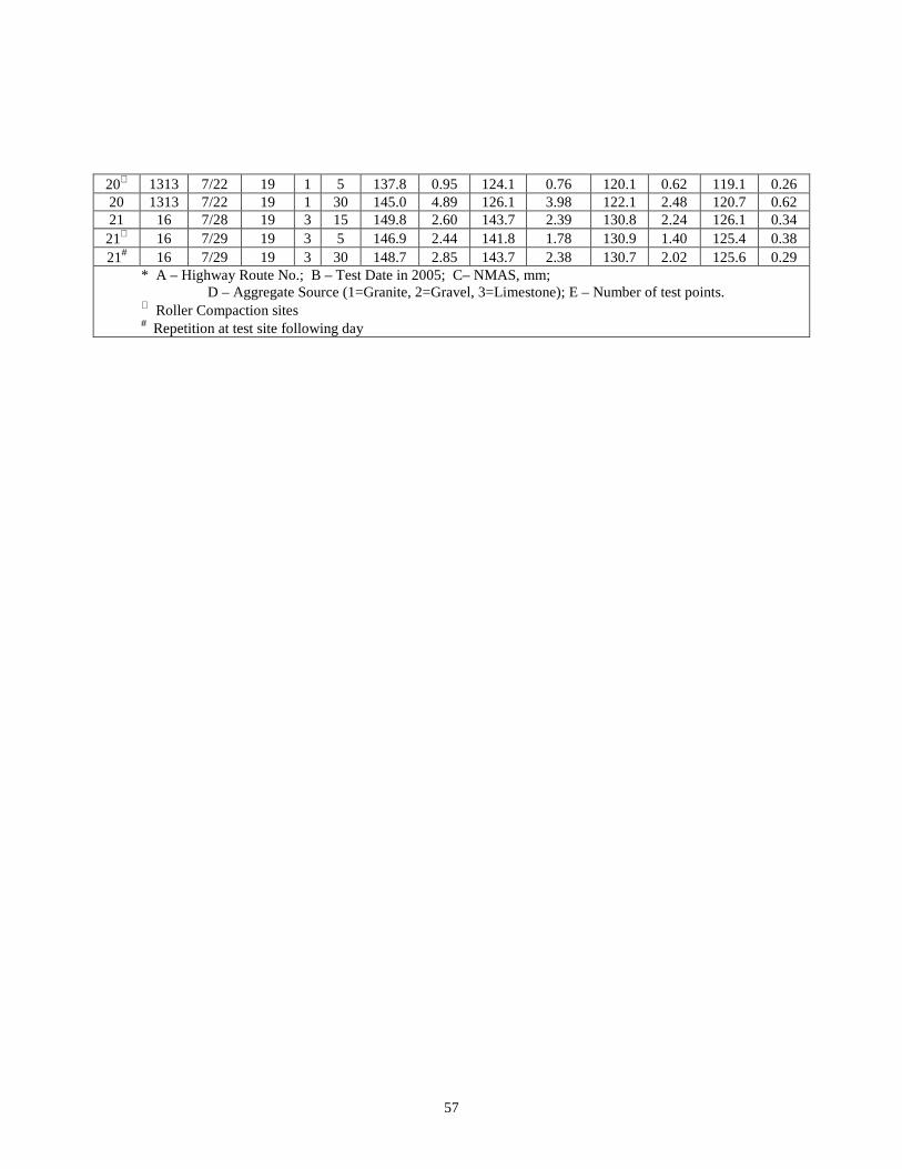
20⊗ 1313 7/22 19 1 5 137.8 0.95 124.1 0.76 120.1 0.62 119.1 0.26 20 1313 7/22 19 1 30 145.0 4.89 126.1 3.98 122.1 2.48 120.7 0.62 21 16 7/28 19 3 15 149.8 2.60 143.7 2.39 130.8 2.24 126.1 0.34 21⊗ 16 7/29 19 3 5 146.9 2.44 141.8 1.78 130.9 1.40 125.4 0.38 21# 16 7/29 19 3 30 148.7 2.85 143.7 2.38 130.7 2.02 125.6 0.29
* A – Highway Route No.; B – Test Date in 2005; C– NMAS, mm; D – Aggregate Source (1=Granite, 2=Gravel, 3=Limestone); E – Number of test points.
⊗ Roller Compaction sites # Repetition at test site following day
57
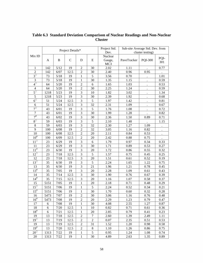
Table 6.3 Standard Deviation Comparison of Nuclear Readings and Non-Nuclear Cluster
Mix ID
Project Details* Project Std.
Dev. Sub-site Average Std. Dev. from
cluster testing)
A B C D E Nuclear Gauge, MC3
PaveTracker PQI-300 PQI301
1 142 5/12 19 2 30 2.02 1.11 . 0.77 2 142 6/07 12.5 2 30 2.40 0.96 0.95 .
3⊗ 73 5/18 19 1 5 3.56 0.70 . 1.01 3 73 5/18 19 1 30 1.35 1.15 . 0.59
4⊗ 64 5/20 19 2 6 1.65 1.03 . 0.53 4 64 5/20 19 2 30 2.25 1.24 . 0.59
5⊗ 1218 5/23 19 3 10 1.82 3.02 . 1.34 5 1218 5/23 19 3 30 2.39 1.92 . 0.68
6⊗ 51 5/24 12.5 3 5 1.97 1.42 . 0.81 6 51 5/24 12.5 3 32 2.31 1.09 . 0.67
7⊗ 43 6/01 19 3 5 1.76 1.08 . 0.72 7 43 6/01 19 3 30 1.99 1.28 . 0.82 7# 43 6/02 19 3 30 2.36 1.50 0.89 0.71 8⊗ 59 6/03 19 3 5 2.10 1.48 . 1.15 8 59 6/03 19 3 32 2.30 1.27 1.09 . 9 100 6/08 19 2 32 3.05 1.16 0.82 .
10 100 6/08 12.5 2 20 2.11 0.84 0.53 . 10# 100 6/09 12.5 2 20 2.42 0.88 0.75 . 11⊗ 23 6/29 19 3 6 1.79 0.97 0.34 0.33 11 23 6/29 19 3 30 1.71 0.89 0.53 0.27 11# 23 6/30 19 3 20 1.72 0.86 0.55 0.32 12⊗ 23 7/18 12.5 3 5 1.57 0.75 0.45 0.25 12 23 7/18 12.5 3 20 1.51 0.61 0.52 0.19
13⊗ 35 6/30 19 3 5 2.24 1.65 1.22 0.75 13 35 6/30 19 3 21 1.96 1.21 0.78 0.45 13# 35 7/05 19 3 20 2.28 1.09 0.61 0.43 14 35 7/14 12.5 3 30 1.90 0.76 0.67 0.39 14# 35 7/15 12.5 3 20 1.16 1.07 0.58 0.37 15 5151 7/05 19 1 20 2.18 0.71 0.48 0.29
15⊗ 5151 7/06 19 1 5 2.24 0.52 0.34 0.21 15# 5151 7/06 19 1 30 1.70 0.60 0.32 0.28 16 5473 7/07 19 2 30 3.06 1.16 0.76 0.48 16# 5473 7/08 19 2 20 2.29 1.23 0.79 0.47 17 6 7/08 19 1 30 4.08 2.55 1.27 0.87 18 6 7/20 12.5 1 10 0.82 0.71 0.61 0.36 18# 6 7/21 12.5 1 20 2.85 0.79 0.41 0.23 19 13 7/18 12.5 2 7 2.60 1.39 2.49 1.11
19⊗ 13 7/19 12.5 2 2 0.07 2.35 0.51 0.53 19 13 7/19 12.5 2 31 1.52 1.20 0.98 0.58 19# 13 7/20 12.5 2 8 1.10 1.26 0.86 0.75 20⊗ 1313 7/22 19 1 5 0.95 1.24 1.08 0.74 20 1313 7/22 19 1 30 4.89 2.63 1.35 0.89
58
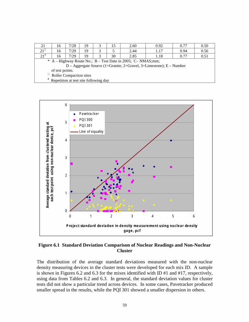
21 16 7/28 19 3 15 2.60 0.92 0.77 0.50 21⊗ 16 7/29 19 3 5 2.44 1.17 0.94 0.56 21# 16 7/29 19 3 30 2.85 1.18 0.77 0.51
* A – Highway Route No.; B – Test Date in 2005; C– NMAS;mm; D – Aggregate Source (1=Granite, 2=Gravel, 3=Limestone); E – Number
of test points. ⊗ Roller Compaction sites # Repetition at test site following day
0
1
2
3
4
5
6
0 1 2 3 4 5 6
Project standard deviation in density measurement using nuclear density gage, pcf
Aver
age
stan
dard
dev
iatio
n fr
om c
lust
ered
test
ing
at
each
test
poi
nt u
sing
non
-nuc
lear
dev
ice,
pcf
Pavetracker
PQI 300
PQI 301
Line of equality
Figure 6.1 Standard Deviation Comparison of Nuclear Readings and Non-Nuclear Cluster
The distribution of the average standard deviations measured with the non-nuclear density measuring devices in the cluster tests were developed for each mix ID. A sample is shown in Figures 6.2 and 6.3 for the mixes identified with ID #1 and #17, respectively, using data from Tables 6.2 and 6.3. In general, the standard deviation values for cluster tests did not show a particular trend across devices. In some cases, Pavetracker produced smaller spread in the results, while the PQI 301 showed a smaller dispersion in others.
59
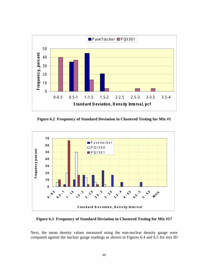
0
10
20
30
40
50
0-0.5 0.5-1 1-1.5 1.5-2 2-2.5 2.5-3 3-3.5 3.5-4
Standard Deviation, Density Interval, pcf
Fre
qu
ency
, per
cen
t PaveTracker PQI-301
Figure 6.2 Frequency of Standard Deviation in Clustered Testing for Mix #1
0
10
20
30
40
50
60
70
0- 0.
5
0.5
- 1
1 1.5
1.5- 2
2- 2.5
2.5
- 3
3- 3.5
3.5- 4
4- 4.
5
4.5
- 5
5 5.
5
More
S tan dard D e v iation , D e n sity In te rv al
Fre
qu
ency
per
cen
t
P a ve tra c k e r
P QI 3 0 0
P QI 3 0 1
Figure 6.3 Frequency of Standard Deviation in Clustered Testing for Mix #17
Next, the mean density values measured using the non-nuclear density gauge were compared against the nuclear gauge readings as shown in Figures 6.4 and 6.5 for mix ID
60
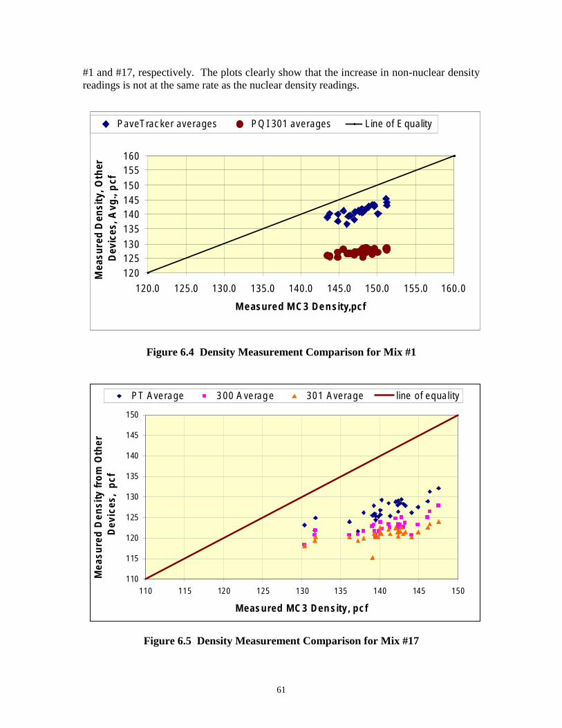
#1 and #17, respectively. The plots clearly show that the increase in non-nuclear density readings is not at the same rate as the nuclear density readings.
120 125 130
135 140 145 150
155 160
120.0 125.0 130.0 135.0 140.0 145.0 150.0 155.0 160.0
Measured MC3 Density,pcf
Mea
sure
d D
ensi
ty, O
ther
Dev
ices
, Avg
., p
cf
PaveTracker averages PQI 301 averages Line of Equality
Figure 6.4 Density Measurement Comparison for Mix #1
110
115
120
125
130
135
140
145
150
110 115 120 125 130 135 140 145 150
Measured MC3 Density, pcf
Mea
sure
d D
ensi
ty fr
om
Oth
erD
evic
es,
pcf
PT Average 300 Average 301 Average line of equality
Figure 6.5 Density Measurement Comparison for Mix #17
61
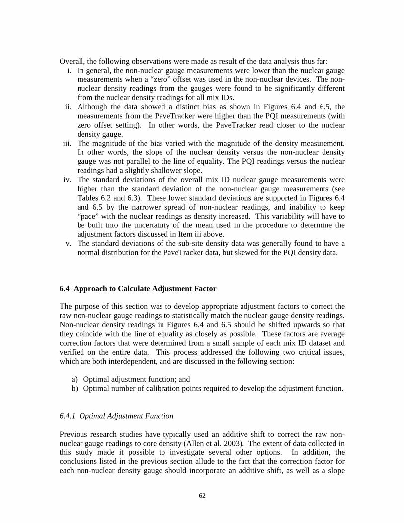
Overall, the following observations were made as result of the data analysis thus far: i. In general, the non-nuclear gauge measurements were lower than the nuclear gauge
measurements when a “zero” offset was used in the non-nuclear devices. The nonnuclear density readings from the gauges were found to be significantly different from the nuclear density readings for all mix IDs.
ii. Although the data showed a distinct bias as shown in Figures 6.4 and 6.5, the measurements from the PaveTracker were higher than the PQI measurements (with zero offset setting). In other words, the PaveTracker read closer to the nuclear density gauge.
iii. The magnitude of the bias varied with the magnitude of the density measurement. In other words, the slope of the nuclear density versus the non-nuclear density gauge was not parallel to the line of equality. The PQI readings versus the nuclear readings had a slightly shallower slope.
iv. The standard deviations of the overall mix ID nuclear gauge measurements were higher than the standard deviation of the non-nuclear gauge measurements (see Tables 6.2 and 6.3). These lower standard deviations are supported in Figures 6.4 and 6.5 by the narrower spread of non-nuclear readings, and inability to keep “pace” with the nuclear readings as density increased. This variability will have to be built into the uncertainty of the mean used in the procedure to determine the adjustment factors discussed in Item iii above.
v. The standard deviations of the sub-site density data was generally found to have a normal distribution for the PaveTracker data, but skewed for the PQI density data.
6.4 Approach to Calculate Adjustment Factor
The purpose of this section was to develop appropriate adjustment factors to correct the raw non-nuclear gauge readings to statistically match the nuclear gauge density readings. Non-nuclear density readings in Figures 6.4 and 6.5 should be shifted upwards so that they coincide with the line of equality as closely as possible. These factors are average correction factors that were determined from a small sample of each mix ID dataset and verified on the entire data. This process addressed the following two critical issues, which are both interdependent, and are discussed in the following section:
a) Optimal adjustment function; and b) Optimal number of calibration points required to develop the adjustment function.
6.4.1 Optimal Adjustment Function
Previous research studies have typically used an additive shift to correct the raw nonnuclear gauge readings to core density (Allen et al. 2003). The extent of data collected in this study made it possible to investigate several other options. In addition, the conclusions listed in the previous section allude to the fact that the correction factor for each non-nuclear density gauge should incorporate an additive shift, as well as a slope
62
term, to closely match the nuclear gauge readings. The goal of the correction factor was to shift the points in Figures 6.4 and 6.5 towards the line of equality. However, it must be verified if using a mere additive or a multiplicative shift will be statistically adequate. Therefore, the accuracy of three different correction functions was investigated:
1. Intercept – Raw non-nuclear readings are adjusted by simply adding a constant correction factor (C1 ), or intercept term, as defined by Equation 6.1:
Corrected Non-nuclear gauge density = Raw non-nuclear reading + C1 ……(6.1)
2. Slope – Raw non-nuclear readings are adjusted by multiplying a constant correction factor (C2), or slope term, as described by Equation 6.2:
Corrected Non-nuclear gauge density = C2*Raw non-nuclear reading …..(6.2)
3. Slope and Intercept – Raw non-nuclear readings are adjusted by multiplying a slope term (C3) and adding an intercept term (C4), as defined by Equation 6.3.
Corrected Non-nuclear gauge density = C3*Raw non-nuclear reading + C4 ...(6.3)
The number of calibration points required to develop the correction factors C1 through C4
was also a key factor in the overall accuracy of the model, as was the form of the model. It was also possible that a less accurate model form can provide reasonably accurate results if sufficiently large number of calibration points are used in the determining the correction constants. The research evaluated these scenarios.
6.4.2 Optimum Number of Calibration Points
In order to establish the correction factors for each mix ID, sets of 3, 5, and 10 random points were investigated as the number of calibration points for field use. The raw nonnuclear density readings were correlated to the corresponding nuclear density readings to develop the correction factors. This correlation resulted in different correction factors for the three different adjustment function types. The number of random points selected from each mix ID for calibrating the non-nuclear gauge readings not only control the accuracy of the device, but also were critical from an implementation standpoint. . The accuracy in predictions of the three sets were compared for three different correction functions. Examples are demonstrated for all 9 combinations of function type and number of calibration points using mix ID #17.
63
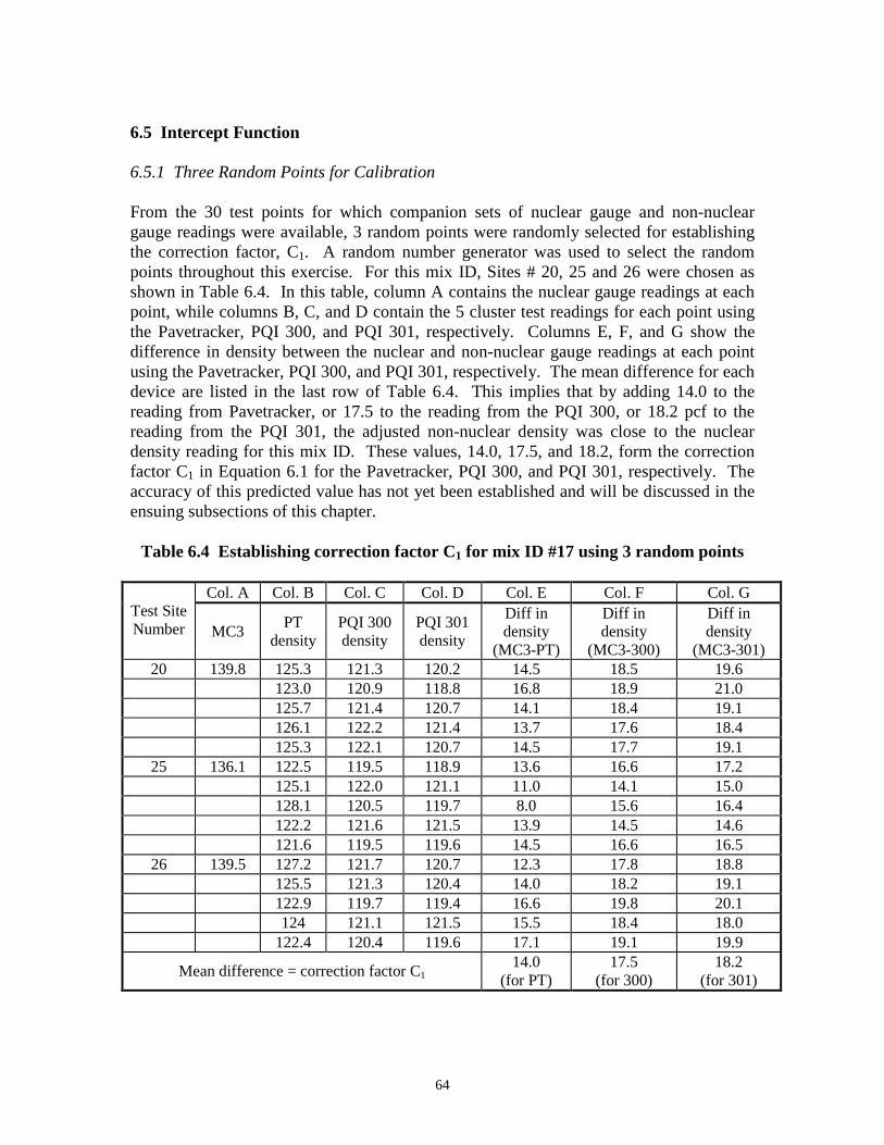
6.5 Intercept Function
6.5.1 Three Random Points for Calibration
From the 30 test points for which companion sets of nuclear gauge and non-nuclear gauge readings were available, 3 random points were randomly selected for establishing the correction factor, C1. A random number generator was used to select the random points throughout this exercise. For this mix ID, Sites # 20, 25 and 26 were chosen as shown in Table 6.4. In this table, column A contains the nuclear gauge readings at each point, while columns B, C, and D contain the 5 cluster test readings for each point using the Pavetracker, PQI 300, and PQI 301, respectively. Columns E, F, and G show the difference in density between the nuclear and non-nuclear gauge readings at each point using the Pavetracker, PQI 300, and PQI 301, respectively. The mean difference for each device are listed in the last row of Table 6.4. This implies that by adding 14.0 to the reading from Pavetracker, or 17.5 to the reading from the PQI 300, or 18.2 pcf to the reading from the PQI 301, the adjusted non-nuclear density was close to the nuclear density reading for this mix ID. These values, 14.0, 17.5, and 18.2, form the correction factor C1 in Equation 6.1 for the Pavetracker, PQI 300, and PQI 301, respectively. The accuracy of this predicted value has not yet been established and will be discussed in the ensuing subsections of this chapter.
Table 6.4 Establishing correction factor C1 for mix ID #17 using 3 random points
Test Site Number
Col. A Col. B Col. C Col. D Col. E Col. F Col. G
MC3 PT
density PQI 300 density
PQI 301 density
Diff in density
(MC3-PT)
Diff in density
(MC3-300)
Diff in density
(MC3-301) 20 139.8 125.3 121.3 120.2 14.5 18.5 19.6
123.0 120.9 118.8 16.8 18.9 21.0 125.7 121.4 120.7 14.1 18.4 19.1 126.1 122.2 121.4 13.7 17.6 18.4 125.3 122.1 120.7 14.5 17.7 19.1
25 136.1 122.5 119.5 118.9 13.6 16.6 17.2 125.1 122.0 121.1 11.0 14.1 15.0 128.1 120.5 119.7 8.0 15.6 16.4 122.2 121.6 121.5 13.9 14.5 14.6 121.6 119.5 119.6 14.5 16.6 16.5
26 139.5 127.2 121.7 120.7 12.3 17.8 18.8 125.5 121.3 120.4 14.0 18.2 19.1 122.9 119.7 119.4 16.6 19.8 20.1 124 121.1 121.5 15.5 18.4 18.0
122.4 120.4 119.6 17.1 19.1 19.9
Mean difference = correction factor C1 14.0
(for PT) 17.5
(for 300) 18.2
(for 301)
64
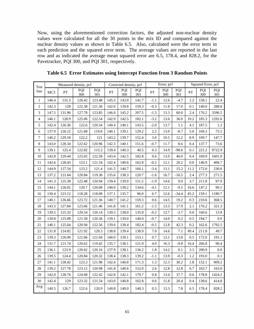
Now, using the aforementioned correction factors, the adjusted non-nuclear density values were calculated for all the 30 points in the mix ID and compared against the nuclear density values as shown in Table 6.5. Also, calculated were the error term in each prediction and the squared error term. The average values are reported in the last row and as indicated the average mean squared error are 6.5, 178.4, and 828.2, for the Pavetracker, PQI 300, and PQI 301, respectively.
Table 6.5 Error Estimates using Intercept Function from 3 Random Points
Test Site
Measured density, pcf Corrected density, pcf Error, pcf Squared Error, pcf
MC3 PT PQI 300
PQI 301
PT PQI 300
PQI 301
PT PQI 300
PQI 301
PT PQI 300
PQI 301
1 146.4 131.3 126.42 123.48 145.3 143.9 141.7 -1.1 12.6 -4.7 1.2 158.1 22.4
2 142.3 128 122.38 121.36 142.0 139.8 159.3 -0.3 11.8 17.0 0.1 140.0 288.8
3 147.5 131.96 127.78 123.85 146.0 145.2 207.5 -1.5 13.3 60.0 2.4 176.2 3596.5
4 146.1 128.9 125.06 122.54 142.9 142.5 182.1 -3.2 13.6 36.0 10.2 185.3 1292.6
5 142.4 126.36 122.6 120.54 140.4 140.1 143.5 -2.0 13.7 1.1 4.1 187.5 1.2
6 137.9 126.12 121.68 119.8 140.1 139.1 129.2 2.2 13.0 -8.7 5.0 169.3 75.5
7 140.2 129.18 122.2 121 143.2 139.7 152.4 3.0 10.5 12.2 8.9 109.7 147.7
8 143.0 128.34 122.62 120.96 142.3 140.1 151.6 -0.7 11.7 8.6 0.4 137.7 73.6
9 139.1 125.4 122.82 115.2 139.4 140.3 40.5 0.3 14.9 -98.6 0.1 221.2 9722.9
10 142.8 129.44 125.02 122.58 143.4 142.5 182.8 0.6 13.0 40.0 0.4 169.9 1601.9
11 142.6 128.43 123.1 121.54 142.4 140.6 162.8 -0.2 12.1 20.2 0.0 146.9 406.7
12 144.9 127.54 123.2 121.4 141.5 140.7 160.1 -3.4 13.1 15.2 11.2 172.0 230.0
13 137.2 121.64 120.84 119.36 135.6 138.3 120.7 -1.6 16.7 -16.5 2.4 277.3 271.5
14 141.3 125.38 122.48 120.94 139.4 139.9 151.2 -1.9 14.6 9.9 3.7 211.8 97.9
15 144.1 126.02 120.7 120.08 140.0 138.2 134.6 -4.1 12.1 -9.5 16.6 147.2 90.1
16 130.4 123.12 118.28 118.08 137.1 135.7 96.0 6.7 12.6 -34.4 45.2 159.1 1180.7
17 140.1 126.66 123.72 121.36 140.7 141.2 159.3 0.6 14.5 19.2 0.3 210.6 368.5
18 143.3 127.84 123.66 121.46 141.8 141.1 161.2 -1.5 13.3 17.9 2.1 176.2 321.3
19 139.5 125.32 120.54 120.14 139.3 138.0 135.8 -0.2 12.7 -3.7 0.0 160.6 13.9
20 139.8 125.08 121.58 120.36 139.1 139.0 140.0 -0.7 14.0 0.2 0.5 194.7 0.0
21 140.1 125.64 120.94 122.56 139.6 138.4 182.4 -0.5 12.8 42.3 0.2 162.6 1792.5
22 131.8 124.82 121.92 120.3 138.8 139.4 138.9 7.0 14.6 7.1 49.4 211.8 49.7
23 139.3 126.00 121.66 121.04 140.0 139.1 153.1 0.7 13.1 13.8 0.5 172.0 191.1
24 131.7 121.74 120.62 119.42 135.7 138.1 121.9 4.0 16.3 -9.8 16.4 266.8 96.4
25 136.1 123.9 120.62 120.16 137.9 138.1 136.2 1.8 14.2 0.1 3.3 200.9 0.0
26 139.5 124.4 120.84 120.32 138.4 138.3 139.2 -1.1 13.9 -0.3 1.2 193.0 0.1
27 141.1 128.42 123.3 121.98 142.4 140.8 171.3 1.3 12.3 30.2 1.8 152.1 909.2
28 139.2 127.78 123.12 120.98 141.8 140.6 152.0 2.6 12.8 12.8 6.7 163.7 163.0
29 142.0 128.76 124.68 122.42 142.8 142.1 179.7 0.8 13.4 37.7 0.6 178.8 1424.2
30 142.4 129 123.32 121.54 143.0 140.8 162.8 0.6 11.8 20.4 0.4 138.6 414.8
Avg .
140.5 126.7 122.6 120.9 140.8 140.0 148.3 0.3 13.3 7.8 6.5 178.4 828.2
65
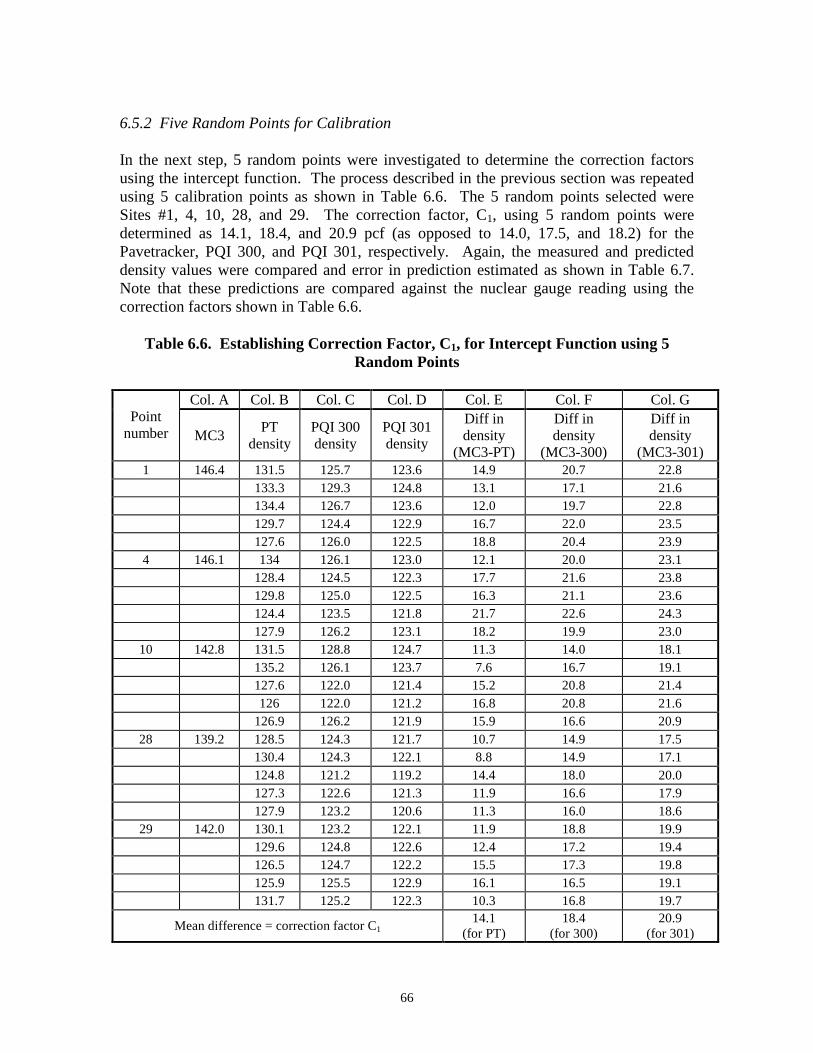
6.5.2 Five Random Points for Calibration
In the next step, 5 random points were investigated to determine the correction factors using the intercept function. The process described in the previous section was repeated using 5 calibration points as shown in Table 6.6. The 5 random points selected were Sites #1, 4, 10, 28, and 29. The correction factor, C1, using 5 random points were determined as 14.1, 18.4, and 20.9 pcf (as opposed to 14.0, 17.5, and 18.2) for the Pavetracker, PQI 300, and PQI 301, respectively. Again, the measured and predicted density values were compared and error in prediction estimated as shown in Table 6.7. Note that these predictions are compared against the nuclear gauge reading using the correction factors shown in Table 6.6.
Table 6.6. Establishing Correction Factor, C1, for Intercept Function using 5 Random Points
Point number
Col. A Col. B Col. C Col. D Col. E Col. F Col. G
MC3 PT
density PQI 300 density
PQI 301 density
Diff in density
(MC3-PT)
Diff in density
(MC3-300)
Diff in density
(MC3-301) 1 146.4 131.5 125.7 123.6 14.9 20.7 22.8
133.3 129.3 124.8 13.1 17.1 21.6 134.4 126.7 123.6 12.0 19.7 22.8 129.7 124.4 122.9 16.7 22.0 23.5 127.6 126.0 122.5 18.8 20.4 23.9
4 146.1 134 126.1 123.0 12.1 20.0 23.1 128.4 124.5 122.3 17.7 21.6 23.8 129.8 125.0 122.5 16.3 21.1 23.6 124.4 123.5 121.8 21.7 22.6 24.3 127.9 126.2 123.1 18.2 19.9 23.0
10 142.8 131.5 128.8 124.7 11.3 14.0 18.1 135.2 126.1 123.7 7.6 16.7 19.1 127.6 122.0 121.4 15.2 20.8 21.4 126 122.0 121.2 16.8 20.8 21.6
126.9 126.2 121.9 15.9 16.6 20.9 28 139.2 128.5 124.3 121.7 10.7 14.9 17.5
130.4 124.3 122.1 8.8 14.9 17.1 124.8 121.2 119.2 14.4 18.0 20.0 127.3 122.6 121.3 11.9 16.6 17.9 127.9 123.2 120.6 11.3 16.0 18.6
29 142.0 130.1 123.2 122.1 11.9 18.8 19.9 129.6 124.8 122.6 12.4 17.2 19.4 126.5 124.7 122.2 15.5 17.3 19.8 125.9 125.5 122.9 16.1 16.5 19.1 131.7 125.2 122.3 10.3 16.8 19.7
Mean difference = correction factor C1 14.1
(for PT) 18.4
(for 300) 20.9
(for 301)
66
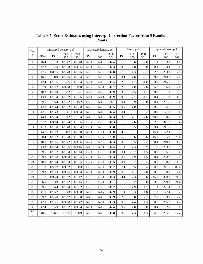
Table 6.7 Error Estimates using Intercept Correction Factor from 5 Random Points
Test #
Measured density, pcf Corrected density, pcf Error, pcf Squared Error, pcf
MC3 PT PQI 300
PQI 301
PT PQI 300
PQI 301
PT PQI 300
PQI 301
PT PQI 300
PQI 301
1 146.4 131.3 126.42 123.48 145.4 144.9 144.4 -1.0 13.6 -2.0 1.1 183.9 4.1
2 142.3 128 122.38 121.36 142.1 140.8 142.3 -0.2 12.8 0.0 0.1 164.4 0.0
3 147.5 131.96 127.78 123.85 146.0 146.2 144.8 -1.5 14.3 -2.7 2.2 203.3 7.5
4 146.1 128.9 125.06 122.54 143.0 143.5 143.4 -3.1 14.6 -2.7 9.8 213.2 7.1
5 142.4 126.36 122.6 120.54 140.4 141.0 141.4 -2.0 14.7 -1.0 3.9 215.5 0.9
6 137.9 126.12 121.68 119.8 140.2 140.1 140.7 2.3 14.0 2.8 5.2 196.0 7.8
7 140.2 129.18 122.2 121 143.2 140.6 141.9 3.0 11.5 1.7 9.3 131.3 2.9
8 143.0 128.34 122.62 120.96 142.4 141.1 141.9 -0.6 12.7 -1.1 0.4 161.8 1.3
9 139.1 125.4 122.82 115.2 139.5 141.3 136.1 0.4 15.9 -3.0 0.1 251.5 9.0
10 142.8 129.44 125.02 122.58 143.5 143.5 143.5 0.7 14.0 0.7 0.5 196.6 0.5
11 142.6 128.43 123.1 121.54 142.5 141.5 142.4 -0.1 13.1 -0.2 0.0 171.8 0.0
12 144.9 127.54 123.2 121.4 141.6 141.6 142.3 -3.3 14.1 -2.6 10.9 198.8 6.8
13 137.2 121.64 120.84 119.36 135.7 139.3 140.3 -1.5 17.6 3.1 2.2 311.2 9.4
14 141.3 125.38 122.48 120.94 139.4 140.9 141.8 -1.9 15.5 0.5 3.4 241.5 0.3
15 144.1 126.02 120.7 120.08 140.1 139.1 141.0 -4.0 13.1 -3.1 16.1 172.1 9.7
16 130.4 123.12 118.28 118.08 137.2 136.7 139.0 6.8 13.6 8.6 46.0 185.0 73.6
17 140.1 126.66 123.72 121.36 140.7 142.2 142.3 0.6 15.5 2.2 0.4 240.3 4.7
18 143.3 127.84 123.66 121.46 141.9 142.1 142.4 -1.4 14.3 -0.9 1.9 203.3 0.9
19 139.5 125.32 120.54 120.14 139.4 139.0 141.0 -0.1 13.7 1.5 0.0 186.6 2.4
20 139.8 125.08 121.58 120.36 139.1 140.0 141.3 -0.7 14.9 1.5 0.4 223.2 2.1
21 140.1 125.64 120.94 122.56 139.7 139.4 143.5 -0.4 13.7 3.4 0.2 188.8 11.3
22 131.8 124.82 121.92 120.3 138.9 140.4 141.2 7.1 15.5 9.4 50.2 241.5 88.4
23 139.3 126.00 121.66 121.04 140.1 140.1 141.9 0.8 14.1 2.6 0.6 198.8 7.0
24 131.7 121.74 120.62 119.42 135.8 139.1 140.3 4.1 17.3 8.6 16.8 300.0 74.3
25 136.1 123.9 120.62 120.16 138.0 139.1 141.1 1.9 15.2 5.0 3.5 229.8 24.6
26 139.5 124.4 120.84 120.32 138.5 139.3 141.2 -1.0 14.9 1.7 1.1 221.4 3.0
27 141.1 128.42 123.3 121.98 142.5 141.7 142.9 1.4 13.3 1.8 1.9 177.4 3.2
28 139.2 127.78 123.12 120.98 141.8 141.6 141.9 2.6 13.8 2.7 7.0 189.9 7.2
29 142.0 128.76 124.68 122.42 142.8 143.1 143.3 0.8 14.4 1.3 0.7 206.2 1.7
30 142.4 129 123.32 121.54 143.1 141.8 142.4 0.7 12.8 0.0 0.4 162.8 0.0
Avg .
140.5 126.7 122.6 120.9 140.8 141.0 141.8 0.3 14.3 1.3 6.5 205.6 12.4
67
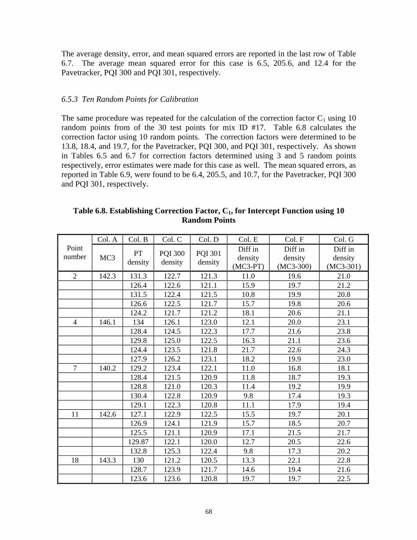
The average density, error, and mean squared errors are reported in the last row of Table 6.7. The average mean squared error for this case is 6.5, 205.6, and 12.4 for the Pavetracker, PQI 300 and PQI 301, respectively.
6.5.3 Ten Random Points for Calibration
The same procedure was repeated for the calculation of the correction factor C1 using 10 random points from of the 30 test points for mix ID #17. Table 6.8 calculates the correction factor using 10 random points. The correction factors were determined to be 13.8, 18.4, and 19.7, for the Pavetracker, PQI 300, and PQI 301, respectively. As shown in Tables 6.5 and 6.7 for correction factors determined using 3 and 5 random points respectively, error estimates were made for this case as well. The mean squared errors, as reported in Table 6.9, were found to be 6.4, 205.5, and 10.7, for the Pavetracker, PQI 300 and PQI 301, respectively.
Table 6.8. Establishing Correction Factor, C1, for Intercept Function using 10 Random Points
Point number
Col. A Col. B Col. C Col. D Col. E Col. F Col. G
MC3 PT
density PQI 300 density
PQI 301 density
Diff in density
(MC3-PT)
Diff in density
(MC3-300)
Diff in density
(MC3-301) 2 142.3 131.3 122.7 121.3 11.0 19.6 21.0
126.4 122.6 121.1 15.9 19.7 21.2 131.5 122.4 121.5 10.8 19.9 20.8 126.6 122.5 121.7 15.7 19.8 20.6 124.2 121.7 121.2 18.1 20.6 21.1
4 146.1 134 126.1 123.0 12.1 20.0 23.1 128.4 124.5 122.3 17.7 21.6 23.8 129.8 125.0 122.5 16.3 21.1 23.6 124.4 123.5 121.8 21.7 22.6 24.3 127.9 126.2 123.1 18.2 19.9 23.0
7 140.2 129.2 123.4 122.1 11.0 16.8 18.1 128.4 121.5 120.9 11.8 18.7 19.3 128.8 121.0 120.3 11.4 19.2 19.9 130.4 122.8 120.9 9.8 17.4 19.3 129.1 122.3 120.8 11.1 17.9 19.4
11 142.6 127.1 122.9 122.5 15.5 19.7 20.1 126.9 124.1 121.9 15.7 18.5 20.7 125.5 121.1 120.9 17.1 21.5 21.7
129.87 122.1 120.0 12.7 20.5 22.6 132.8 125.3 122.4 9.8 17.3 20.2
18 143.3 130 121.2 120.5 13.3 22.1 22.8 128.7 123.9 121.7 14.6 19.4 21.6 123.6 123.6 120.8 19.7 19.7 22.5
68
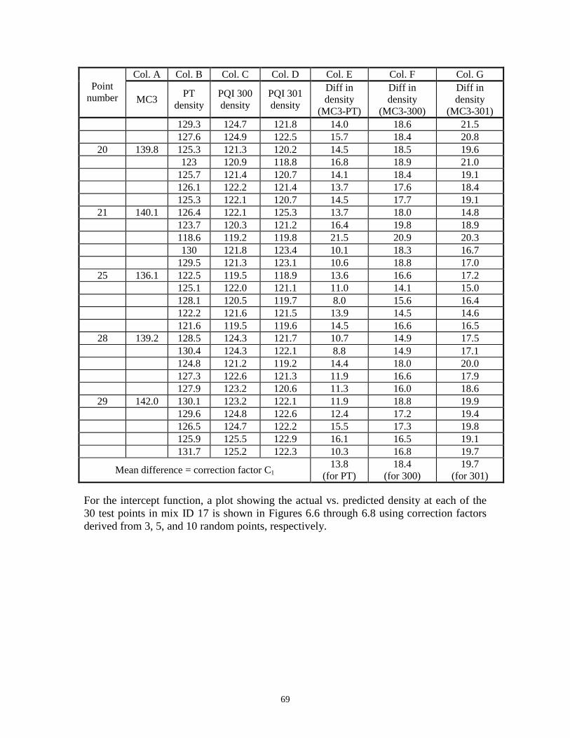
Point number
Col. A Col. B Col. C Col. D Col. E Col. F Col. G
MC3 PT
density PQI 300 density
PQI 301 density
Diff in density
(MC3-PT)
Diff in density
(MC3-300)
Diff in density
(MC3-301) 129.3 124.7 121.8 14.0 18.6 21.5 127.6 124.9 122.5 15.7 18.4 20.8
20 139.8 125.3 121.3 120.2 14.5 18.5 19.6 123 120.9 118.8 16.8 18.9 21.0
125.7 121.4 120.7 14.1 18.4 19.1 126.1 122.2 121.4 13.7 17.6 18.4 125.3 122.1 120.7 14.5 17.7 19.1
21 140.1 126.4 122.1 125.3 13.7 18.0 14.8 123.7 120.3 121.2 16.4 19.8 18.9 118.6 119.2 119.8 21.5 20.9 20.3 130 121.8 123.4 10.1 18.3 16.7
129.5 121.3 123.1 10.6 18.8 17.0 25 136.1 122.5 119.5 118.9 13.6 16.6 17.2
125.1 122.0 121.1 11.0 14.1 15.0 128.1 120.5 119.7 8.0 15.6 16.4 122.2 121.6 121.5 13.9 14.5 14.6 121.6 119.5 119.6 14.5 16.6 16.5
28 139.2 128.5 124.3 121.7 10.7 14.9 17.5 130.4 124.3 122.1 8.8 14.9 17.1 124.8 121.2 119.2 14.4 18.0 20.0 127.3 122.6 121.3 11.9 16.6 17.9 127.9 123.2 120.6 11.3 16.0 18.6
29 142.0 130.1 123.2 122.1 11.9 18.8 19.9 129.6 124.8 122.6 12.4 17.2 19.4 126.5 124.7 122.2 15.5 17.3 19.8 125.9 125.5 122.9 16.1 16.5 19.1 131.7 125.2 122.3 10.3 16.8 19.7
Mean difference = correction factor C1 13.8
(for PT) 18.4
(for 300) 19.7
(for 301)
For the intercept function, a plot showing the actual vs. predicted density at each of the 30 test points in mix ID 17 is shown in Figures 6.6 through 6.8 using correction factors derived from 3, 5, and 10 random points, respectively.
69
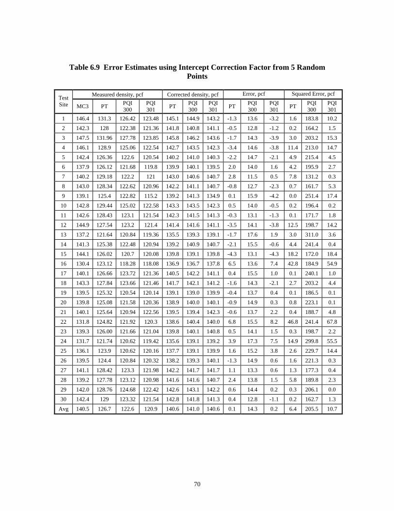
Table 6.9 Error Estimates using Intercept Correction Factor from 5 Random Points
Test Site
Measured density, pcf Corrected density, pcf Error, pcf Squared Error, pcf
MC3 PT PQI 300
PQI 301
PT PQI 300
PQI 301
PT PQI 300
PQI 301
PT PQI 300
PQI 301
1 146.4 131.3 126.42 123.48 145.1 144.9 143.2 -1.3 13.6 -3.2 1.6 183.8 10.2
2 142.3 128 122.38 121.36 141.8 140.8 141.1 -0.5 12.8 -1.2 0.2 164.2 1.5
3 147.5 131.96 127.78 123.85 145.8 146.2 143.6 -1.7 14.3 -3.9 3.0 203.2 15.3
4 146.1 128.9 125.06 122.54 142.7 143.5 142.3 -3.4 14.6 -3.8 11.4 213.0 14.7
5 142.4 126.36 122.6 120.54 140.2 141.0 140.3 -2.2 14.7 -2.1 4.9 215.4 4.5
6 137.9 126.12 121.68 119.8 139.9 140.1 139.5 2.0 14.0 1.6 4.2 195.9 2.7
7 140.2 129.18 122.2 121 143.0 140.6 140.7 2.8 11.5 0.5 7.8 131.2 0.3
8 143.0 128.34 122.62 120.96 142.2 141.1 140.7 -0.8 12.7 -2.3 0.7 161.7 5.3
9 139.1 125.4 122.82 115.2 139.2 141.3 134.9 0.1 15.9 -4.2 0.0 251.4 17.4
10 142.8 129.44 125.02 122.58 143.3 143.5 142.3 0.5 14.0 -0.5 0.2 196.4 0.2
11 142.6 128.43 123.1 121.54 142.3 141.5 141.3 -0.3 13.1 -1.3 0.1 171.7 1.8
12 144.9 127.54 123.2 121.4 141.4 141.6 141.1 -3.5 14.1 -3.8 12.5 198.7 14.2
13 137.2 121.64 120.84 119.36 135.5 139.3 139.1 -1.7 17.6 1.9 3.0 311.0 3.6
14 141.3 125.38 122.48 120.94 139.2 140.9 140.7 -2.1 15.5 -0.6 4.4 241.4 0.4
15 144.1 126.02 120.7 120.08 139.8 139.1 139.8 -4.3 13.1 -4.3 18.2 172.0 18.4
16 130.4 123.12 118.28 118.08 136.9 136.7 137.8 6.5 13.6 7.4 42.8 184.9 54.9
17 140.1 126.66 123.72 121.36 140.5 142.2 141.1 0.4 15.5 1.0 0.1 240.1 1.0
18 143.3 127.84 123.66 121.46 141.7 142.1 141.2 -1.6 14.3 -2.1 2.7 203.2 4.4
19 139.5 125.32 120.54 120.14 139.1 139.0 139.9 -0.4 13.7 0.4 0.1 186.5 0.1
20 139.8 125.08 121.58 120.36 138.9 140.0 140.1 -0.9 14.9 0.3 0.8 223.1 0.1
21 140.1 125.64 120.94 122.56 139.5 139.4 142.3 -0.6 13.7 2.2 0.4 188.7 4.8
22 131.8 124.82 121.92 120.3 138.6 140.4 140.0 6.8 15.5 8.2 46.8 241.4 67.8
23 139.3 126.00 121.66 121.04 139.8 140.1 140.8 0.5 14.1 1.5 0.3 198.7 2.2
24 131.7 121.74 120.62 119.42 135.6 139.1 139.2 3.9 17.3 7.5 14.9 299.8 55.5
25 136.1 123.9 120.62 120.16 137.7 139.1 139.9 1.6 15.2 3.8 2.6 229.7 14.4
26 139.5 124.4 120.84 120.32 138.2 139.3 140.1 -1.3 14.9 0.6 1.6 221.3 0.3
27 141.1 128.42 123.3 121.98 142.2 141.7 141.7 1.1 13.3 0.6 1.3 177.3 0.4
28 139.2 127.78 123.12 120.98 141.6 141.6 140.7 2.4 13.8 1.5 5.8 189.8 2.3
29 142.0 128.76 124.68 122.42 142.6 143.1 142.2 0.6 14.4 0.2 0.3 206.1 0.0
30 142.4 129 123.32 121.54 142.8 141.8 141.3 0.4 12.8 -1.1 0.2 162.7 1.3
Avg 140.5 126.7 122.6 120.9 140.6 141.0 140.6 0.1 14.3 0.2 6.4 205.5 10.7
70
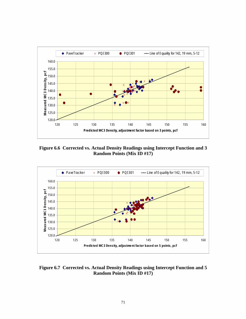
120.0
125.0
130.0
135.0
140.0
145.0
150.0
155.0
160.0
120 125 130 135 140 145 150 155 160
Predicted MC3 Density, adjustment factor based on 3 points, pcf
Mea
sure
d M
C3
Den
sity
, pcf
PaveTracker PQI 300 PQI301 Line of Equality for 142, 19 mm, 5-12
Figure 6.6 Corrected vs. Actual Density Readings using Intercept Function and 3 Random Points (Mix ID #17)
120.0
125.0
130.0
135.0
140.0
145.0
150.0
155.0
160.0
120 125 130 135 140 145 150 155 160
Predicted MC3 Density, adjustment factor based on 5 points, pcf
Mea
sure
d M
C3
Den
sity
, pcf
PaveTracker PQI300 PQI301 Line of Equality for 142, 19 mm, 5-12
Figure 6.7 Corrected vs. Actual Density Readings using Intercept Function and 5 Random Points (Mix ID #17)
71
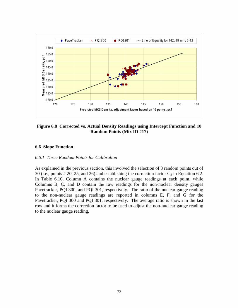
120.0
125.0
130.0
135.0
140.0
145.0
150.0
155.0
160.0
120 125 130 135 140 145 150 155 160
Predicted MC3 Density, adjustment factor based on 10 points, pcf
Mea
sure
d M
C3
Den
sity
, pcf
PaveTracker PQI300 PQI 301 Line of Equality for 142, 19 mm, 5-12
Figure 6.8 Corrected vs. Actual Density Readings using Intercept Function and 10 Random Points (Mix ID #17)
6.6 Slope Function
6.6.1 Three Random Points for Calibration
As explained in the previous section, this involved the selection of 3 random points out of 30 (i.e., points # 20, 25, and 26) and establishing the correction factor C2 in Equation 6.2. In Table 6.10, Column A contains the nuclear gauge readings at each point, while Columns B, C, and D contain the raw readings for the non-nuclear density gauges Pavetracker, PQI 300, and PQI 301, respectively. The ratio of the nuclear gauge reading to the non-nuclear gauge readings are reported in columns E, F, and G for the Pavetracker, PQI 300 and PQI 301, respectively. The average ratio is shown in the last row and it forms the correction factor to be used to adjust the non-nuclear gauge reading to the nuclear gauge reading.
72
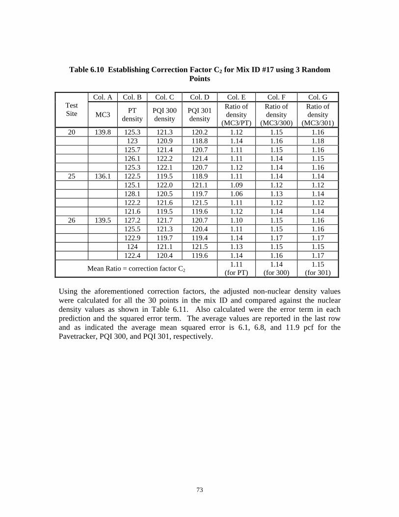
Table 6.10 Establishing Correction Factor C2 for Mix ID #17 using 3 Random Points
Test Site
Col. A Col. B Col. C Col. D Col. E Col. F Col. G
MC3 PT
density PQI 300 density
PQI 301 density
Ratio of density
(MC3/PT)
Ratio of density
(MC3/300)
Ratio of density
(MC3/301) 20 139.8 125.3 121.3 120.2 1.12 1.15 1.16
123 120.9 118.8 1.14 1.16 1.18 125.7 121.4 120.7 1.11 1.15 1.16 126.1 122.2 121.4 1.11 1.14 1.15 125.3 122.1 120.7 1.12 1.14 1.16
25 136.1 122.5 119.5 118.9 1.11 1.14 1.14 125.1 122.0 121.1 1.09 1.12 1.12 128.1 120.5 119.7 1.06 1.13 1.14 122.2 121.6 121.5 1.11 1.12 1.12 121.6 119.5 119.6 1.12 1.14 1.14
26 139.5 127.2 121.7 120.7 1.10 1.15 1.16 125.5 121.3 120.4 1.11 1.15 1.16 122.9 119.7 119.4 1.14 1.17 1.17 124 121.1 121.5 1.13 1.15 1.15
122.4 120.4 119.6 1.14 1.16 1.17
Mean Ratio = correction factor C2 1.11
(for PT) 1.14
(for 300) 1.15
(for 301)
Using the aforementioned correction factors, the adjusted non-nuclear density values were calculated for all the 30 points in the mix ID and compared against the nuclear density values as shown in Table 6.11. Also calculated were the error term in each prediction and the squared error term. The average values are reported in the last row and as indicated the average mean squared error is 6.1, 6.8, and 11.9 pcf for the Pavetracker, PQI 300, and PQI 301, respectively.
73
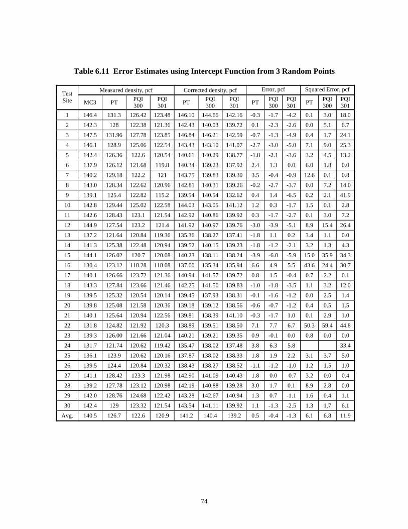
Table 6.11 Error Estimates using Intercept Function from 3 Random Points
Test Site
Measured density, pcf Corrected density, pcf Error, pcf Squared Error, pcf
MC3 PT PQI 300
PQI 301
PT PQI 300
PQI 301
PT PQI 300
PQI 301
PT PQI 300
PQI 301
1 146.4 131.3 126.42 123.48 146.10 144.66 142.16 -0.3 -1.7 -4.2 0.1 3.0 18.0
2 142.3 128 122.38 121.36 142.43 140.03 139.72 0.1 -2.3 -2.6 0.0 5.1 6.7
3 147.5 131.96 127.78 123.85 146.84 146.21 142.59 -0.7 -1.3 -4.9 0.4 1.7 24.1
4 146.1 128.9 125.06 122.54 143.43 143.10 141.07 -2.7 -3.0 -5.0 7.1 9.0 25.3
5 142.4 126.36 122.6 120.54 140.61 140.29 138.77 -1.8 -2.1 -3.6 3.2 4.5 13.2
6 137.9 126.12 121.68 119.8 140.34 139.23 137.92 2.4 1.3 0.0 6.0 1.8 0.0
7 140.2 129.18 122.2 121 143.75 139.83 139.30 3.5 -0.4 -0.9 12.6 0.1 0.8
8 143.0 128.34 122.62 120.96 142.81 140.31 139.26 -0.2 -2.7 -3.7 0.0 7.2 14.0
9 139.1 125.4 122.82 115.2 139.54 140.54 132.62 0.4 1.4 -6.5 0.2 2.1 41.9
10 142.8 129.44 125.02 122.58 144.03 143.05 141.12 1.2 0.3 -1.7 1.5 0.1 2.8
11 142.6 128.43 123.1 121.54 142.92 140.86 139.92 0.3 -1.7 -2.7 0.1 3.0 7.2
12 144.9 127.54 123.2 121.4 141.92 140.97 139.76 -3.0 -3.9 -5.1 8.9 15.4 26.4
13 137.2 121.64 120.84 119.36 135.36 138.27 137.41 -1.8 1.1 0.2 3.4 1.1 0.0
14 141.3 125.38 122.48 120.94 139.52 140.15 139.23 -1.8 -1.2 -2.1 3.2 1.3 4.3
15 144.1 126.02 120.7 120.08 140.23 138.11 138.24 -3.9 -6.0 -5.9 15.0 35.9 34.3
16 130.4 123.12 118.28 118.08 137.00 135.34 135.94 6.6 4.9 5.5 43.6 24.4 30.7
17 140.1 126.66 123.72 121.36 140.94 141.57 139.72 0.8 1.5 -0.4 0.7 2.2 0.1
18 143.3 127.84 123.66 121.46 142.25 141.50 139.83 -1.0 -1.8 -3.5 1.1 3.2 12.0
19 139.5 125.32 120.54 120.14 139.45 137.93 138.31 -0.1 -1.6 -1.2 0.0 2.5 1.4
20 139.8 125.08 121.58 120.36 139.18 139.12 138.56 -0.6 -0.7 -1.2 0.4 0.5 1.5
21 140.1 125.64 120.94 122.56 139.81 138.39 141.10 -0.3 -1.7 1.0 0.1 2.9 1.0
22 131.8 124.82 121.92 120.3 138.89 139.51 138.50 7.1 7.7 6.7 50.3 59.4 44.8
23 139.3 126.00 121.66 121.04 140.21 139.21 139.35 0.9 -0.1 0.0 0.8 0.0 0.0
24 131.7 121.74 120.62 119.42 135.47 138.02 137.48 3.8 6.3 5.8 33.4
25 136.1 123.9 120.62 120.16 137.87 138.02 138.33 1.8 1.9 2.2 3.1 3.7 5.0
26 139.5 124.4 120.84 120.32 138.43 138.27 138.52 -1.1 -1.2 -1.0 1.2 1.5 1.0
27 141.1 128.42 123.3 121.98 142.90 141.09 140.43 1.8 0.0 -0.7 3.2 0.0 0.4
28 139.2 127.78 123.12 120.98 142.19 140.88 139.28 3.0 1.7 0.1 8.9 2.8 0.0
29 142.0 128.76 124.68 122.42 143.28 142.67 140.94 1.3 0.7 -1.1 1.6 0.4 1.1
30 142.4 129 123.32 121.54 143.54 141.11 139.92 1.1 -1.3 -2.5 1.3 1.7 6.1
Avg. 140.5 126.7 122.6 120.9 141.2 140.4 139.2 0.5 -0.4 -1.3 6.1 6.8 11.9
74
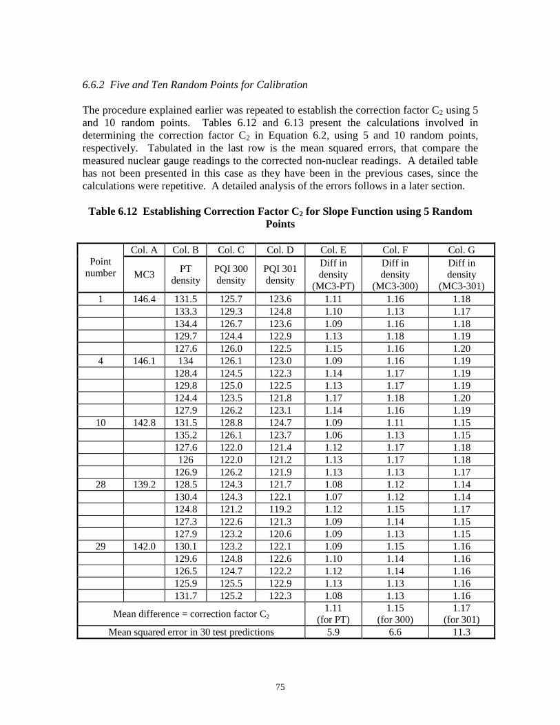
6.6.2 Five and Ten Random Points for Calibration
The procedure explained earlier was repeated to establish the correction factor C2 using 5 and 10 random points. Tables 6.12 and 6.13 present the calculations involved in determining the correction factor C2 in Equation 6.2, using 5 and 10 random points, respectively. Tabulated in the last row is the mean squared errors, that compare the measured nuclear gauge readings to the corrected non-nuclear readings. A detailed table has not been presented in this case as they have been in the previous cases, since the calculations were repetitive. A detailed analysis of the errors follows in a later section.
Table 6.12 Establishing Correction Factor C2 for Slope Function using 5 Random Points
Point number
Col. A Col. B Col. C Col. D Col. E Col. F Col. G
MC3 PT
density PQI 300 density
PQI 301 density
Diff in density
(MC3-PT)
Diff in density
(MC3-300)
Diff in density
(MC3-301) 1 146.4 131.5 125.7 123.6 1.11 1.16 1.18
133.3 129.3 124.8 1.10 1.13 1.17 134.4 126.7 123.6 1.09 1.16 1.18 129.7 124.4 122.9 1.13 1.18 1.19 127.6 126.0 122.5 1.15 1.16 1.20
4 146.1 134 126.1 123.0 1.09 1.16 1.19 128.4 124.5 122.3 1.14 1.17 1.19 129.8 125.0 122.5 1.13 1.17 1.19 124.4 123.5 121.8 1.17 1.18 1.20 127.9 126.2 123.1 1.14 1.16 1.19
10 142.8 131.5 128.8 124.7 1.09 1.11 1.15 135.2 126.1 123.7 1.06 1.13 1.15 127.6 122.0 121.4 1.12 1.17 1.18 126 122.0 121.2 1.13 1.17 1.18
126.9 126.2 121.9 1.13 1.13 1.17 28 139.2 128.5 124.3 121.7 1.08 1.12 1.14
130.4 124.3 122.1 1.07 1.12 1.14 124.8 121.2 119.2 1.12 1.15 1.17 127.3 122.6 121.3 1.09 1.14 1.15 127.9 123.2 120.6 1.09 1.13 1.15
29 142.0 130.1 123.2 122.1 1.09 1.15 1.16 129.6 124.8 122.6 1.10 1.14 1.16 126.5 124.7 122.2 1.12 1.14 1.16 125.9 125.5 122.9 1.13 1.13 1.16 131.7 125.2 122.3 1.08 1.13 1.16
Mean difference = correction factor C2 1.11
(for PT) 1.15
(for 300) 1.17
(for 301) Mean squared error in 30 test predictions 5.9 6.6 11.3
75
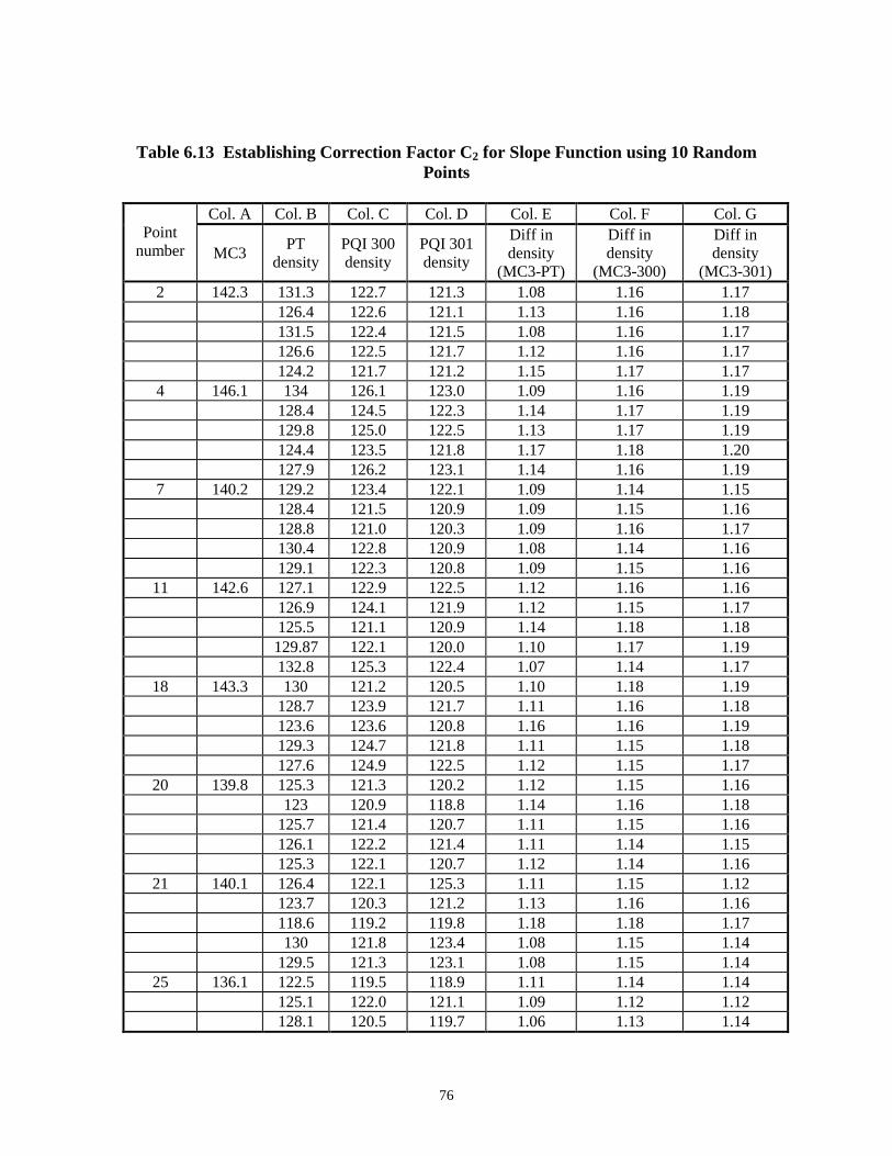
Table 6.13 Establishing Correction Factor C2 for Slope Function using 10 Random Points
Point number
Col. A Col. B Col. C Col. D Col. E Col. F Col. G
MC3 PT
density PQI 300 density
PQI 301 density
Diff in density
(MC3-PT)
Diff in density
(MC3-300)
Diff in density
(MC3-301) 2 142.3 131.3 122.7 121.3 1.08 1.16 1.17
126.4 122.6 121.1 1.13 1.16 1.18 131.5 122.4 121.5 1.08 1.16 1.17 126.6 122.5 121.7 1.12 1.16 1.17 124.2 121.7 121.2 1.15 1.17 1.17
4 146.1 134 126.1 123.0 1.09 1.16 1.19 128.4 124.5 122.3 1.14 1.17 1.19 129.8 125.0 122.5 1.13 1.17 1.19 124.4 123.5 121.8 1.17 1.18 1.20 127.9 126.2 123.1 1.14 1.16 1.19
7 140.2 129.2 123.4 122.1 1.09 1.14 1.15 128.4 121.5 120.9 1.09 1.15 1.16 128.8 121.0 120.3 1.09 1.16 1.17 130.4 122.8 120.9 1.08 1.14 1.16 129.1 122.3 120.8 1.09 1.15 1.16
11 142.6 127.1 122.9 122.5 1.12 1.16 1.16 126.9 124.1 121.9 1.12 1.15 1.17 125.5 121.1 120.9 1.14 1.18 1.18
129.87 122.1 120.0 1.10 1.17 1.19 132.8 125.3 122.4 1.07 1.14 1.17
18 143.3 130 121.2 120.5 1.10 1.18 1.19 128.7 123.9 121.7 1.11 1.16 1.18 123.6 123.6 120.8 1.16 1.16 1.19 129.3 124.7 121.8 1.11 1.15 1.18 127.6 124.9 122.5 1.12 1.15 1.17
20 139.8 125.3 121.3 120.2 1.12 1.15 1.16 123 120.9 118.8 1.14 1.16 1.18
125.7 121.4 120.7 1.11 1.15 1.16 126.1 122.2 121.4 1.11 1.14 1.15 125.3 122.1 120.7 1.12 1.14 1.16
21 140.1 126.4 122.1 125.3 1.11 1.15 1.12 123.7 120.3 121.2 1.13 1.16 1.16 118.6 119.2 119.8 1.18 1.18 1.17 130 121.8 123.4 1.08 1.15 1.14
129.5 121.3 123.1 1.08 1.15 1.14 25 136.1 122.5 119.5 118.9 1.11 1.14 1.14
125.1 122.0 121.1 1.09 1.12 1.12 128.1 120.5 119.7 1.06 1.13 1.14
76
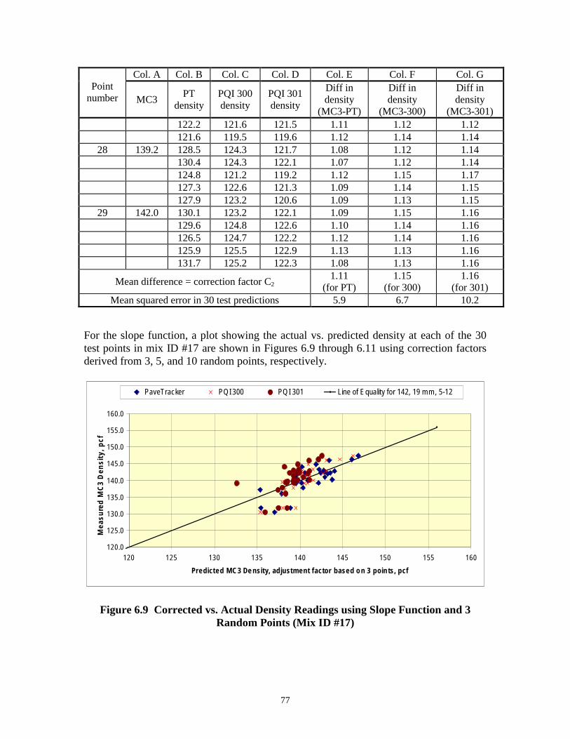
Point number
Col. A Col. B Col. C Col. D Col. E Col. F Col. G
MC3 PT
density PQI 300 density
PQI 301 density
Diff in density
(MC3-PT)
Diff in density
(MC3-300)
Diff in density
(MC3-301) 122.2 121.6 121.5 1.11 1.12 1.12 121.6 119.5 119.6 1.12 1.14 1.14
28 139.2 128.5 124.3 121.7 1.08 1.12 1.14 130.4 124.3 122.1 1.07 1.12 1.14 124.8 121.2 119.2 1.12 1.15 1.17 127.3 122.6 121.3 1.09 1.14 1.15 127.9 123.2 120.6 1.09 1.13 1.15
29 142.0 130.1 123.2 122.1 1.09 1.15 1.16 129.6 124.8 122.6 1.10 1.14 1.16 126.5 124.7 122.2 1.12 1.14 1.16 125.9 125.5 122.9 1.13 1.13 1.16 131.7 125.2 122.3 1.08 1.13 1.16
Mean difference = correction factor C2 1.11
(for PT) 1.15
(for 300) 1.16
(for 301) Mean squared error in 30 test predictions 5.9 6.7 10.2
For the slope function, a plot showing the actual vs. predicted density at each of the 30 test points in mix ID #17 are shown in Figures 6.9 through 6.11 using correction factors derived from 3, 5, and 10 random points, respectively.
120.0
125.0
130.0
135.0
140.0
145.0
150.0
155.0
160.0
120 125 130 135 140 145 150 155 160
Predicted MC3 Density, adjustment factor based on 3 points, pcf
Mea
sure
d M
C3
Den
sity
, pcf
PaveTracker PQI300 PQI 301 Line of Equality for 142, 19 mm, 5-12
Figure 6.9 Corrected vs. Actual Density Readings using Slope Function and 3 Random Points (Mix ID #17)
77
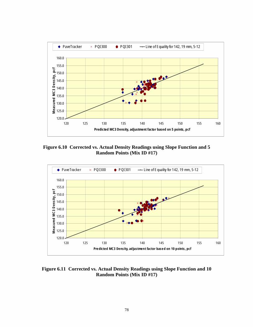
120.0
125.0
130.0
135.0
140.0
145.0
150.0
155.0
160.0
120 125 130 135 140 145 150 155 160
Predicted MC3 Density, adjustment factor based on 5 points, pcf
Mea
sure
d M
C3
Den
sity
, pcf
PaveTracker PQI300 PQI301 Lineof Equalityfor 142, 19 mm, 5-12
Figure 6.10 Corrected vs. Actual Density Readings using Slope Function and 5 Random Points (Mix ID #17)
120.0
125.0
130.0
135.0
140.0
145.0
150.0
155.0
160.0
120 125 130 135 140 145 150 155 160
Predicted MC3 Density, adjustment factor based on 10 points, pcf
Mea
sure
d M
C3
Den
sity
, pcf
PaveTracker PQI300 PQI301 Line of Equality for 142, 19 mm, 5-12
Figure 6.11 Corrected vs. Actual Density Readings using Slope Function and 10 Random Points (Mix ID #17)
78
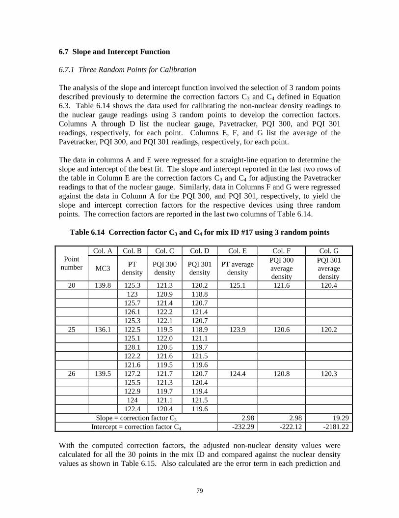
6.7 Slope and Intercept Function
6.7.1 Three Random Points for Calibration
The analysis of the slope and intercept function involved the selection of 3 random points described previously to determine the correction factors C3 and C4 defined in Equation 6.3. Table 6.14 shows the data used for calibrating the non-nuclear density readings to the nuclear gauge readings using 3 random points to develop the correction factors. Columns A through D list the nuclear gauge, Pavetracker, PQI 300, and PQI 301 readings, respectively, for each point. Columns E, F, and G list the average of the Pavetracker, PQI 300, and PQI 301 readings, respectively, for each point.
The data in columns A and E were regressed for a straight-line equation to determine the slope and intercept of the best fit. The slope and intercept reported in the last two rows of the table in Column E are the correction factors C3 and C4 for adjusting the Pavetracker readings to that of the nuclear gauge. Similarly, data in Columns F and G were regressed against the data in Column A for the PQI 300, and PQI 301, respectively, to yield the slope and intercept correction factors for the respective devices using three random points. The correction factors are reported in the last two columns of Table 6.14.
Table 6.14 Correction factor C3 and C4 for mix ID #17 using 3 random points
Point number
Col. A Col. B Col. C Col. D Col. E Col. F Col. G
MC3 PT
density PQI 300 density
PQI 301 density
PT average density
PQI 300 average density
PQI 301 average density
20 139.8 125.3 121.3 120.2 125.1 121.6 120.4 123 120.9 118.8
125.7 121.4 120.7 126.1 122.2 121.4 125.3 122.1 120.7
25 136.1 122.5 119.5 118.9 123.9 120.6 120.2 125.1 122.0 121.1 128.1 120.5 119.7 122.2 121.6 121.5 121.6 119.5 119.6
26 139.5 127.2 121.7 120.7 124.4 120.8 120.3 125.5 121.3 120.4 122.9 119.7 119.4 124 121.1 121.5
122.4 120.4 119.6 Slope = correction factor C3 2.98 2.98 19.29
Intercept = correction factor C4 -232.29 -222.12 -2181.22
With the computed correction factors, the adjusted non-nuclear density values were calculated for all the 30 points in the mix ID and compared against the nuclear density values as shown in Table 6.15. Also calculated are the error term in each prediction and
79
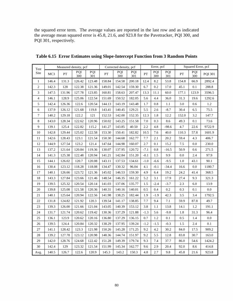
the squared error term. The average values are reported in the last row and as indicated the average mean squared error is 45.8, 21.6, and 923.8 for the Pavetracker, PQI 300, and PQI 301, respectively.
Table 6.15 Error Estimates using Slope-Intercept Function from 3 Random Points
Test Site
Measured density, pcf Corrected density, pcf Error, pcf Squared Error, pcf
MC3 PT PQI 300
PQI 301
PT PQI 300
PQI 301
PT PQI 300
PQI 301
PT PQI 300
PQI 301
1 146.4 131.3 126.42 123.48 158.84 154.58 200.18 12.4 8.2 53.8 154.8 66.9 2892.4
2 142.3 128 122.38 121.36 149.01 142.54 159.30 6.7 0.2 17.0 45.1 0.1 288.8
3 147.5 131.96 127.78 123.85 160.81 158.63 207.47 13.3 11.1 60.0 177.1 123.9 3596.5
4 146.1 128.9 125.06 122.54 151.69 150.52 182.05 5.6 4.4 36.0 31.3 19.6 1292.6
5 142.4 126.36 122.6 120.54 144.13 143.19 143.48 1.7 0.8 1.1 3.0 0.6 1.2
6 137.9 126.12 121.68 119.8 143.41 140.45 129.21 5.5 2.6 -8.7 30.4 6.5 75.5
7 140.2 129.18 122.2 121 152.53 142.00 152.35 12.3 1.8 12.2 152.0 3.2 147.7
8 143.0 128.34 122.62 120.96 150.02 143.25 151.58 7.0 0.3 8.6 49.3 0.1 73.6
9 139.1 125.4 122.82 115.2 141.27 143.85 40.50 2.2 4.8 -98.6 4.7 22.6 9722.9
10 142.8 129.44 125.02 122.58 153.30 150.41 182.82 10.5 7.6 40.0 110.3 57.8 1601.9
11 142.6 128.43 123.1 121.54 150.30 144.68 162.77 7.7 2.1 20.2 59.4 4.3 406.7
12 144.9 127.54 123.2 121.4 147.64 144.98 160.07 2.7 0.1 15.2 7.5 0.0 230.0
13 137.2 121.64 120.84 119.36 130.07 137.95 120.72 -7.1 0.8 -16.5 50.9 0.6 271.5
14 141.3 125.38 122.48 120.94 141.21 142.84 151.20 -0.1 1.5 9.9 0.0 2.4 97.9
15 144.1 126.02 120.7 120.08 143.11 137.53 134.61 -1.0 -6.6 -9.5 1.0 43.1 90.1
16 130.4 123.12 118.28 118.08 134.47 130.32 96.04 4.1 -0.1 -34.4 16.6 0.0 1180.7
17 140.1 126.66 123.72 121.36 145.02 146.53 159.30 4.9 6.4 19.2 24.2 41.4 368.5
18 143.3 127.84 123.66 121.46 148.54 146.35 161.22 5.2 3.1 17.9 27.4 9.3 321.3
19 139.5 125.32 120.54 120.14 141.03 137.06 135.77 1.5 -2.4 -3.7 2.3 6.0 13.9
20 139.8 125.08 121.58 120.36 140.31 140.16 140.01 0.5 0.4 0.2 0.3 0.1 0.0
21 140.1 125.64 120.94 122.56 141.98 138.25 182.44 1.9 -1.9 42.3 3.5 3.4 1792.5
22 131.8 124.82 121.92 120.3 139.54 141.17 138.85 7.7 9.4 7.1 59.9 87.8 49.7
23 139.3 126.00 121.66 121.04 143.05 140.39 153.12 3.8 1.1 13.8 14.1 1.2 191.1
24 131.7 121.74 120.62 119.42 130.36 137.29 121.88 -1.3 5.6 -9.8 1.8 31.3 96.4
25 136.1 123.9 120.62 120.16 136.80 137.29 136.15 0.7 1.2 0.1 0.5 1.4 0.0
26 139.5 124.4 120.84 120.32 138.29 137.95 139.24 -1.2 -1.5 -0.3 1.5 2.4 0.1
27 141.1 128.42 123.3 121.98 150.26 145.28 171.25 9.2 4.2 30.2 84.0 17.5 909.2
28 139.2 127.78 123.12 120.98 148.36 144.74 151.97 9.2 5.5 12.8 83.8 30.7 163.0
29 142.0 128.76 124.68 122.42 151.28 149.39 179.74 9.3 7.4 37.7 86.0 54.6 1424.2
30 142.4 129 123.32 121.54 151.99 145.34 162.77 9.6 2.9 20.4 92.0 8.6 414.8
Avg. 140.5 126.7 122.6 120.9 145.3 143.2 150.3 4.8 2.7 9.8 45.8 21.6 923.8
80
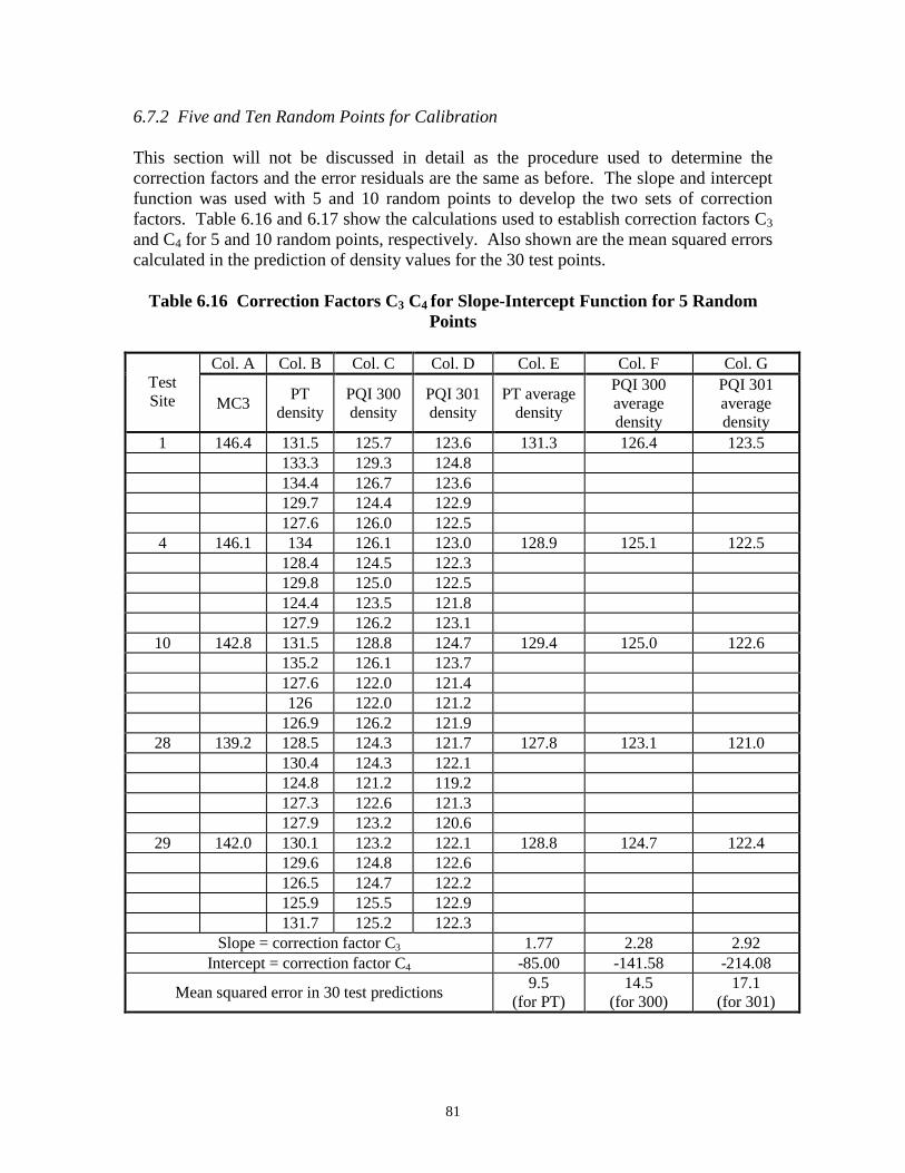
6.7.2 Five and Ten Random Points for Calibration
This section will not be discussed in detail as the procedure used to determine the correction factors and the error residuals are the same as before. The slope and intercept function was used with 5 and 10 random points to develop the two sets of correction factors. Table 6.16 and 6.17 show the calculations used to establish correction factors C3
and C4 for 5 and 10 random points, respectively. Also shown are the mean squared errors calculated in the prediction of density values for the 30 test points.
Table 6.16 Correction Factors C3 C4 for Slope-Intercept Function for 5 Random Points
Test Site
Col. A Col. B Col. C Col. D Col. E Col. F Col. G
MC3 PT
density PQI 300 density
PQI 301 density
PT average density
PQI 300 average density
PQI 301 average density
1 146.4 131.5 125.7 123.6 131.3 126.4 123.5 133.3 129.3 124.8 134.4 126.7 123.6 129.7 124.4 122.9 127.6 126.0 122.5
4 146.1 134 126.1 123.0 128.9 125.1 122.5 128.4 124.5 122.3 129.8 125.0 122.5 124.4 123.5 121.8 127.9 126.2 123.1
10 142.8 131.5 128.8 124.7 129.4 125.0 122.6 135.2 126.1 123.7 127.6 122.0 121.4 126 122.0 121.2
126.9 126.2 121.9 28 139.2 128.5 124.3 121.7 127.8 123.1 121.0
130.4 124.3 122.1 124.8 121.2 119.2 127.3 122.6 121.3 127.9 123.2 120.6
29 142.0 130.1 123.2 122.1 128.8 124.7 122.4 129.6 124.8 122.6 126.5 124.7 122.2 125.9 125.5 122.9 131.7 125.2 122.3
Slope = correction factor C3 1.77 2.28 2.92 Intercept = correction factor C4 -85.00 -141.58 -214.08
Mean squared error in 30 test predictions 9.5
(for PT) 14.5
(for 300) 17.1
(for 301)
81
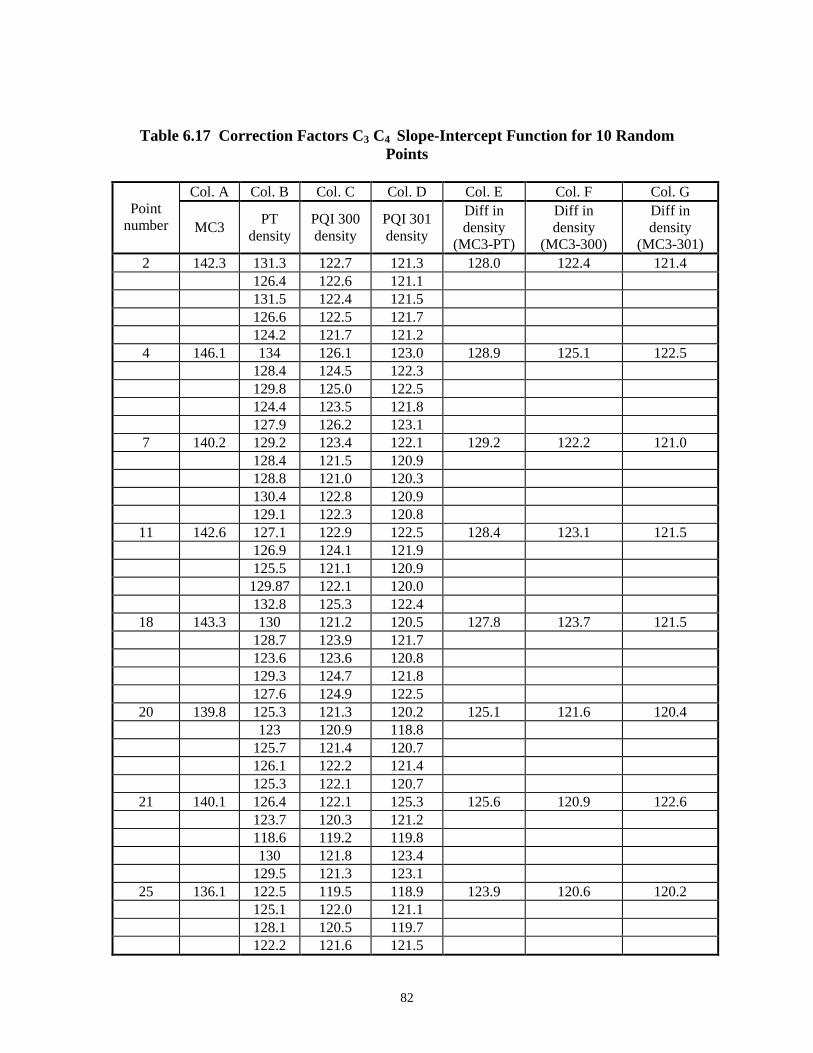
Table 6.17 Correction Factors C3 C4 Slope-Intercept Function for 10 Random Points
Point number
Col. A Col. B Col. C Col. D Col. E Col. F Col. G
MC3 PT
density PQI 300 density
PQI 301 density
Diff in density
(MC3-PT)
Diff in density
(MC3-300)
Diff in density
(MC3-301) 2 142.3 131.3 122.7 121.3 128.0 122.4 121.4
126.4 122.6 121.1 131.5 122.4 121.5 126.6 122.5 121.7 124.2 121.7 121.2
4 146.1 134 126.1 123.0 128.9 125.1 122.5 128.4 124.5 122.3 129.8 125.0 122.5 124.4 123.5 121.8 127.9 126.2 123.1
7 140.2 129.2 123.4 122.1 129.2 122.2 121.0 128.4 121.5 120.9 128.8 121.0 120.3 130.4 122.8 120.9 129.1 122.3 120.8
11 142.6 127.1 122.9 122.5 128.4 123.1 121.5 126.9 124.1 121.9 125.5 121.1 120.9 129.87 122.1 120.0 132.8 125.3 122.4
18 143.3 130 121.2 120.5 127.8 123.7 121.5 128.7 123.9 121.7 123.6 123.6 120.8 129.3 124.7 121.8 127.6 124.9 122.5
20 139.8 125.3 121.3 120.2 125.1 121.6 120.4 123 120.9 118.8
125.7 121.4 120.7 126.1 122.2 121.4 125.3 122.1 120.7
21 140.1 126.4 122.1 125.3 125.6 120.9 122.6 123.7 120.3 121.2 118.6 119.2 119.8 130 121.8 123.4
129.5 121.3 123.1 25 136.1 122.5 119.5 118.9 123.9 120.6 120.2
125.1 122.0 121.1 128.1 120.5 119.7 122.2 121.6 121.5
82
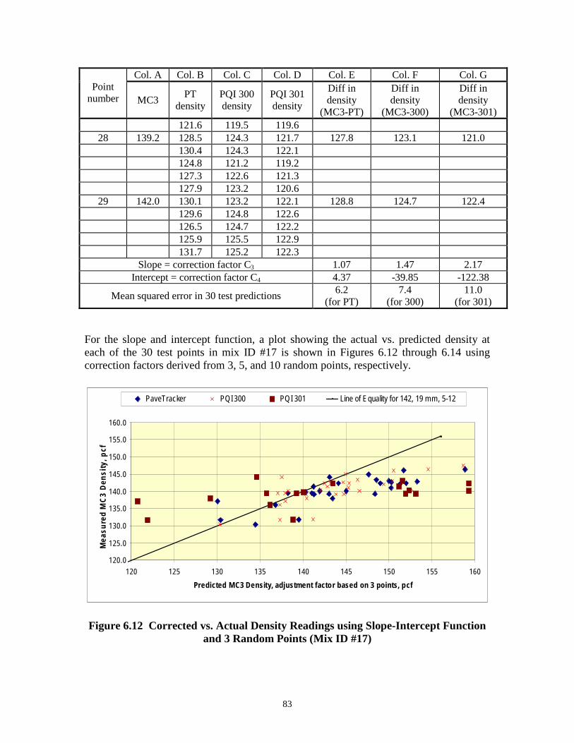
Point number
Col. A Col. B Col. C Col. D Col. E Col. F Col. G
MC3 PT
density PQI 300 density
PQI 301 density
Diff in density
(MC3-PT)
Diff in density
(MC3-300)
Diff in density
(MC3-301) 121.6 119.5 119.6
28 139.2 128.5 124.3 121.7 127.8 123.1 121.0 130.4 124.3 122.1 124.8 121.2 119.2 127.3 122.6 121.3 127.9 123.2 120.6
29 142.0 130.1 123.2 122.1 128.8 124.7 122.4 129.6 124.8 122.6 126.5 124.7 122.2 125.9 125.5 122.9 131.7 125.2 122.3
Slope = correction factor C3 1.07 1.47 2.17 Intercept = correction factor C4 4.37 -39.85 -122.38
Mean squared error in 30 test predictions 6.2
(for PT) 7.4
(for 300) 11.0
(for 301)
For the slope and intercept function, a plot showing the actual vs. predicted density at each of the 30 test points in mix ID #17 is shown in Figures 6.12 through 6.14 using correction factors derived from 3, 5, and 10 random points, respectively.
120.0
125.0
130.0
135.0
140.0
145.0
150.0
155.0
160.0
120 125 130 135 140 145 150 155 160
Predicted MC3 Density, adjustment factor based on 3 points, pcf
Mea
sure
d M
C3
Den
sity
, pcf
PaveTracker PQI300 PQI 301 Lineof Equality for 142, 19mm, 5-12
Figure 6.12 Corrected vs. Actual Density Readings using Slope-Intercept Function and 3 Random Points (Mix ID #17)
83
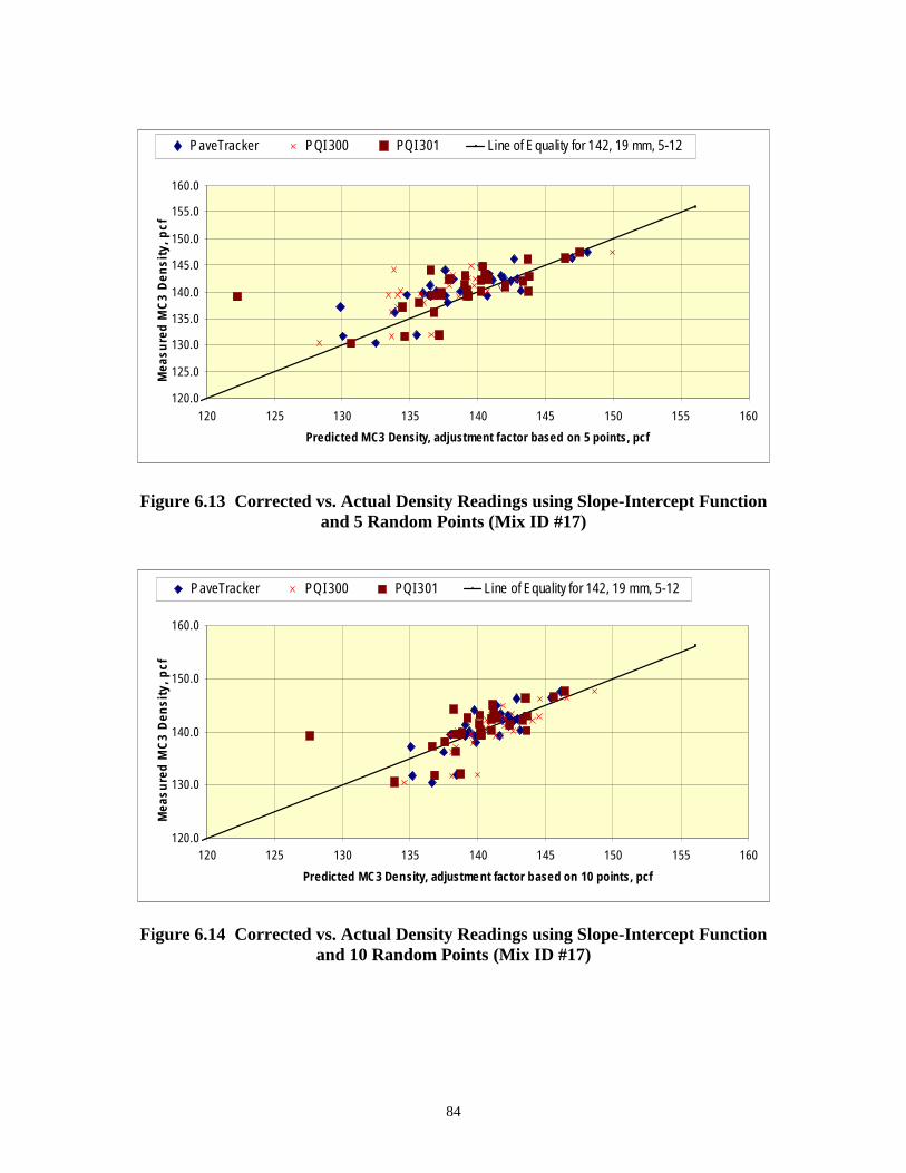
120.0
125.0
130.0
135.0
140.0
145.0
150.0
155.0
160.0
120 125 130 135 140 145 150 155 160
Predicted MC3 Density, adjustment factor based on 5 points, pcf
Mea
sure
d M
C3
Den
sity
, pcf
PaveTracker PQI300 PQI301 Line of Equality for 142, 19 mm, 5-12
Figure 6.13 Corrected vs. Actual Density Readings using Slope-Intercept Function and 5 Random Points (Mix ID #17)
120.0
130.0
140.0
150.0
160.0
120 125 130 135 140 145 150 155 160
Predicted MC3 Density, adjustment factor based on 10 points, pcf
Mea
sure
d M
C3
Den
sity
, pcf
PaveTracker PQI300 PQI301 Line of Equalityfor 142, 19 mm, 5-12
Figure 6.14 Corrected vs. Actual Density Readings using Slope-Intercept Function and 10 Random Points (Mix ID #17)
84
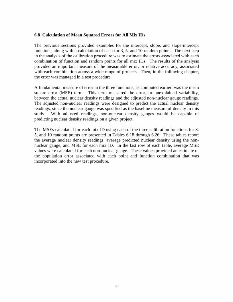
6.8 Calculation of Mean Squared Errors for All Mix IDs
The previous sections provided examples for the intercept, slope, and slope-intercept functions, along with a calculation of each for 3, 5, and 10 random points. The next step in the analysis of the calibration procedure was to estimate the errors associated with each combination of function and random points for all mix IDs. The results of the analysis provided an important measure of the measurable error, or relative accuracy, associated with each combination across a wide range of projects. Then, in the following chapter, the error was managed in a test procedure.
A fundamental measure of error in the three functions, as computed earlier, was the mean square error (MSE) term. This term measured the error, or unexplained variability, between the actual nuclear density readings and the adjusted non-nuclear gauge readings. The adjusted non-nuclear readings were designed to predict the actual nuclear density readings, since the nuclear gauge was specified as the baseline measure of density in this study. With adjusted readings, non-nuclear density gauges would be capable of predicting nuclear density readings on a given project.
The MSEs calculated for each mix ID using each of the three calibration functions for 3, 5, and 10 random points are presented in Tables 6.18 through 6.26. These tables report the average nuclear density readings, average predicted nuclear density using the nonnuclear gauge, and MSE for each mix ID. In the last row of each table, average MSE values were calculated for each non-nuclear gauge. These values provided an estimate of the population error associated with each point and function combination that was incorporated into the new test procedure.
85
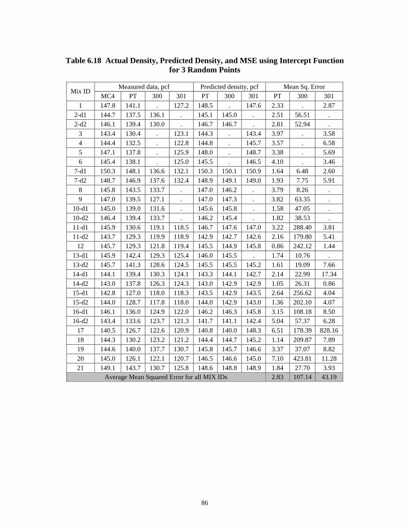
Table 6.18 Actual Density, Predicted Density, and MSE using Intercept Function for 3 Random Points
Mix ID Measured data, pcf Predicted density, pcf Mean Sq. Error
MC4 PT 300 301 PT 300 301 PT 300 301
1 147.8 141.1 . 127.2 148.5 . 147.6 2.33 . 2.87
2-d1 144.7 137.5 136.1 . 145.1 145.0 . 2.51 56.51 .
2-d2 146.1 139.4 130.0 . 146.7 146.7 . 2.81 52.94 .
3 143.4 130.4 . 123.1 144.3 . 143.4 3.97 . 3.58
4 144.4 132.5 . 122.8 144.8 . 145.7 3.57 . 6.58
5 147.1 137.8 . 125.9 148.0 . 148.7 3.38 . 5.69
6 145.4 138.1 . 125.0 145.5 . 146.5 4.10 . 3.46
7-d1 150.3 148.1 136.6 132.1 150.3 150.1 150.9 1.64 6.48 2.60
7-d2 148.7 146.9 137.6 132.4 148.9 149.1 149.0 1.93 7.75 5.91
8 145.8 143.5 133.7 . 147.0 146.2 . 3.79 8.26 .
9 147.0 139.5 127.1 . 147.0 147.3 . 3.82 63.35 .
10-d1 145.0 139.0 131.6 . 145.6 145.8 . 1.58 47.05 .
10-d2 146.4 139.4 133.7 . 146.2 145.4 . 1.82 38.53 .
11-d1 145.9 130.6 119.1 118.5 146.7 147.6 147.0 3.22 288.40 3.81
11-d2 143.7 129.3 119.9 118.9 142.9 142.7 142.6 2.16 179.80 5.41
12 145.7 129.3 121.8 119.4 145.5 144.9 145.8 0.86 242.12 1.44
13-d1 145.9 142.4 129.3 125.4 146.0 145.5 . 1.74 10.76 .
13-d2 145.7 141.3 128.6 124.5 145.5 145.5 145.2 1.61 19.09 7.66
14-d1 144.1 139.4 130.3 124.1 143.3 144.1 142.7 2.14 22.99 17.34
14-d2 143.0 137.8 126.3 124.3 143.0 142.9 142.9 1.05 26.31 0.86
15-d1 142.8 127.0 118.0 118.3 143.5 142.9 143.5 2.64 256.62 4.04
15-d2 144.0 128.7 117.8 118.0 144.0 142.9 143.0 1.36 202.10 4.07
16-d1 146.1 136.0 124.9 122.0 146.2 146.3 145.8 3.15 108.18 8.50 16-d2 143.4 133.6 123.7 121.3 141.7 141.1 142.4 5.04 57.37 6.28
17 140.5 126.7 122.6 120.9 140.8 140.0 148.3 6.51 178.39 828.16
18 144.3 130.2 123.2 121.2 144.4 144.7 145.2 1.14 209.87 7.89
19 144.6 140.0 137.7 130.7 145.8 145.7 146.6 3.37 37.07 8.82
20 145.0 126.1 122.1 120.7 146.5 146.6 145.0 7.10 423.81 11.28
21 149.1 143.7 130.7 125.8 148.6 148.8 148.9 1.84 27.70 3.93 Average Mean Squared Error for all MIX IDs 2.83 107.14 43.19
86
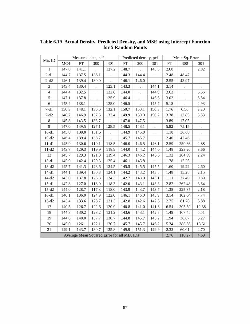
Table 6.19 Actual Density, Predicted Density, and MSE using Intercept Function for 5 Random Points
Mix ID Measured data, pcf Predicted density, pcf Mean Sq. Error
MC4 PT 300 301 PT 300 301 PT 300 301
1 147.8 141.1 . 127.2 148.7 . 148.3 2.60 . 2.82
2-d1 144.7 137.5 136.1 . 144.3 144.4 . 2.48 48.47 .
2-d2 146.1 139.4 130.0 . 146.1 146.0 . 2.55 43.97 .
3 143.4 130.4 . 123.1 143.3 . 144.1 3.14 . .
4 144.4 132.5 . 122.8 144.0 . 144.9 3.63 . 5.56
5 147.1 137.8 . 125.9 146.4 . 146.6 3.02 . 3.84
6 145.4 138.1 . 125.0 146.5 . 145.7 5.18 . 2.93
7-d1 150.3 148.1 136.6 132.1 150.7 150.1 150.3 1.76 6.56 2.20
7-d2 148.7 146.9 137.6 132.4 149.9 150.0 150.2 3.38 12.85 5.83
8 145.8 143.5 133.7 . 147.0 147.5 . 3.89 17.05 .
9 147.0 139.5 127.1 128.5 148.5 148.1 . 5.82 75.15 .
10-d1 145.0 139.0 131.6 . 144.9 145.0 . 1.18 36.68 .
10-d2 146.4 139.4 133.7 . 145.7 145.7 . 2.40 42.46 .
11-d1 145.9 130.6 119.1 118.5 146.0 146.5 146.1 2.59 250.66 2.88
11-d2 143.7 129.3 119.9 118.9 144.0 144.2 144.0 1.48 223.20 3.66
12 145.7 129.3 121.8 119.4 146.3 146.2 146.6 1.32 284.99 2.24
13-d1 145.9 142.4 129.3 125.4 146.1 145.8 . 1.78 12.25 .
13-d2 145.7 141.3 128.6 124.5 145.5 145.5 145.5 1.60 19.22 2.60
14-d1 144.1 139.4 130.3 124.1 144.2 143.2 143.8 1.48 15.28 2.15
14-d2 143.0 137.8 126.3 124.3 142.7 143.0 143.1 1.11 27.49 0.89
15-d1 142.8 127.0 118.0 118.3 142.0 143.1 143.3 2.82 262.48 3.64
15-d2 144.0 128.7 117.8 118.0 143.9 143.7 143.7 1.38 225.37 2.18
16-d1 146.1 136.0 124.9 122.0 146.1 146.0 145.9 3.14 102.04 7.74
16-d2 143.4 133.6 123.7 121.3 142.8 142.6 142.8 2.75 81.78 5.88
17 140.5 126.7 122.6 120.9 140.8 141.0 141.8 6.54 205.59 12.38
18 144.3 130.2 123.2 121.2 143.6 143.1 142.8 1.49 167.45 5.51
19 144.6 140.0 137.7 130.7 144.8 145.7 145.2 1.94 36.67 5.27
20 145.0 126.1 122.1 120.7 145.7 145.7 146.2 5.34 388.66 13.61
21 149.1 143.7 130.7 125.8 149.9 151.3 149.9 2.33 60.01 4.70 Average Mean Squared Error for all MIX IDs 2.76 110.27 4.69
87
Table 6.20 Actual Density, Predicted Density, and MSE using Intercept Function for 10 Random Points
Mix ID Measured data, pcf Predicted density, pcf Mean Sq. Error
MC4 PT 300 301 PT 300 301 PT 300 301
1 147.8 141.1 . 127.2 147.7 . 148.3 1.75 . 2.89
2-d1 144.7 137.5 136.1 . 144.4 144.4 . 2.36 48.45 .
2-d2 146.1 139.4 130.0 . 146.3 146.0 . 2.56 43.24 .
3 143.4 130.4 . 123.1 142.9 . 143.1 3.44 . 1.62
4 144.4 132.5 . 122.8 144.5 . 144.5 3.44 . 5.38
5 147.1 137.8 . 125.9 147.3 . 147.1 2.55 . 3.62
6 145.4 138.1 . 125.0 145.6 . 146.0 4.12 . 3.14
7-d1 150.3 148.1 136.6 132.1 150.0 150.2 149.9 1.73 6.92 2.41
7-d2 148.7 146.9 137.6 132.4 149.6 150.2 149.9 2.78 13.87 5.07
8 145.8 143.5 133.7 . 145.6 145.7 . 2.39 5.95 .
9 147.0 139.5 127.1 128.5 146.8 146.7 . 3.88 54.25 .
10-d1 145.0 139.0 131.6 . 145.1 144.9 . 1.20 35.73 .
10-d2 146.4 139.4 133.7 . 146.3 146.0 . 1.80 46.11 .
11-d1 145.9 130.6 119.1 118.5 146.3 146.8 146.6 2.70 262.56 3.24
11-d2 143.7 129.3 119.9 118.9 144.0 144.2 144.4 1.49 221.49 4.02
12 145.7 129.3 121.8 119.4 146.0 145.8 146.0 0.95 271.92 1.48
13-d1 145.9 142.4 129.3 125.4 146.0 145.7 . 1.74 11.68 .
13-d2 145.7 141.3 128.6 124.5 146.0 145.4 145.2 1.66 17.91 2.77
14-d1 144.1 139.4 130.3 124.1 143.8 144.4 144.2 1.54 25.14 2.06
14-d2 143.0 137.8 126.3 124.3 143.5 143.0 142.9 1.30 27.66 0.89
15-d1 142.8 127.0 118.0 118.3 143.1 142.2 142.0 2.23 236.22 4.12
15-d2 144.0 128.7 117.8 118.0 144.5 144.1 144.1 1.56 236.54 2.10
16-d1 146.1 136.0 124.9 122.0 145.4 144.4 144.2 3.65 73.05 11.18
16-d2 143.4 133.6 123.7 121.3 143.2 142.6 142.8 2.42 83.25 5.80
17 140.5 126.7 122.6 120.9 140.6 141.0 140.6 6.44 205.48 10.66
18 144.3 130.2 123.2 121.2 144.6 144.7 144.9 1.23 211.27 3.68
19 144.6 140.0 137.7 130.7 144.2 144.9 144.6 2.14 28.80 4.92
20 145.0 126.1 122.1 120.7 144.3 144.3 144.3 5.44 335.74 12.83
21 149.1 143.7 130.7 125.8 149.1 148.7 148.9 1.66 27.58 3.94 Average Mean Squared Error for all MIX IDs 2.49 105.45 4.45
88

Table 6.21 Actual Density, Predicted Density, and MSE using Slope Function for 3 Random Points
Mix ID Measured data, pcf Predicted density, pcf Mean Sq. Error
MC4 PT 300 301 PT 300 301 PT 300 301
1 147.8 141.1 . 127.2 148.6 . 147.5 2.52 . 2.58
2-d1 144.7 137.5 136.1 . 145.1 144.9 . 2.43 3.94 .
2-d2 146.1 139.4 130.0 . 146.7 146.6 . 2.85 2.98 .
3 143.4 130.4 . 123.1 144.4 . 144.2 4.67 . 2.18
4 144.4 132.5 . 122.8 144.8 . . 3.68 . .
5 147.1 137.8 . 125.9 147.9 . 148.9 3.21 . 6.69
6 145.4 138.1 . 125.0 145.4 . 146.9 4.42 . 4.92
7-d1 150.3 148.1 136.6 132.1 150.3 150.0 150.8 1.67 2.54 2.40
7-d2 148.7 146.9 137.6 132.4 149.0 149.2 149.1 1.67 6.88 4.33
8 145.8 143.5 133.7 . 147.1 146.4 . 4.10 3.92 .
9 147.0 139.5 127.1 128.5 147.0 147.4 . 3.79 4.10 .
10-d1 145.0 139.0 131.6 . 145.6 145.7 . 1.50 1.33 .
10-d2 146.4 139.4 133.7 . 146.2 145.3 . 1.80 4.06 .
11-d1 145.9 130.6 119.1 118.5 146.7 147.8 147.3 3.34 8.38 4.88
11-d2 143.7 129.3 119.9 118.9 142.9 142.7 142.6 2.10 5.75 5.37
12 145.7 129.3 121.8 119.4 145.6 144.9 144.9 0.81 1.35 1.86
13-d1 145.9 142.4 129.3 125.4 146.0 145.5 145.8 1.74 1.63 1.77
13-d2 145.7 141.3 128.6 124.5 145.5 145.5 145.4 1.62 1.55 2.43
14-d1 144.1 139.4 130.3 124.1 143.3 144.2 143.6 2.16 1.71 2.19
14-d2 143.0 137.8 126.3 124.3 143.0 142.9 142.9 1.10 0.70 0.86
15-d1 142.8 127.0 118.0 118.3 143.5 142.8 143.5 3.13 2.38 3.77
15-d2 144.0 128.7 117.8 118.0 144.2 143.0 142.7 1.43 2.27 3.84
16-d1 146.1 136.0 124.9 122.0 146.2 146.4 146.4 3.18 7.43 7.86 16-d2 143.4 133.6 123.7 121.3 141.7 140.9 141.3 5.03 14.18 9.96
17 140.5 126.7 122.6 120.9 141.0 140.3 139.2 6.41 7.89 11.92
18 144.3 130.2 123.2 121.2 144.4 144.6 144.6 0.95 2.35 3.23
19 144.6 140.0 137.7 130.7 145.7 149.5 148.3 3.14 30.89 19.29
20 145.0 126.1 122.1 120.7 146.3 146.2 147.2 6.32 8.47 15.34
21 149.1 143.7 130.7 125.8 148.7 148.9 148.4 1.79 4.42 4.05 Average Mean Squared Error for all MIX IDs 2.85 5.46 5.53
89

Table 6.22 Actual Density, Predicted Density, and MSE using Slope Function for 5 Random Points
Mix ID Measured data, pcf Predicted density, pcf Mean Sq. Error
MC4 PT 300 301 PT 300 301 PT 300 301
1 147.8 141.1 . 127.2 148.7 . 148.3 2.76 . 2.77
2-d1 144.7 137.5 136.1 . 144.3 144.4 . 2.43 3.95 .
2-d2 146.1 139.4 130.0 . 146.1 146.0 . 2.55 2.84 .
3 143.4 130.4 . 123.1 143.3 . 144.1 3.66 . 2.07
4 144.4 132.5 . 122.8 144.0 . . 3.72 . .
5 147.1 137.8 . 125.9 146.3 . 146.5 3.08 . 3.75
6 145.4 138.1 . 125.0 146.5 . 145.6 5.60 . 2.66
7-d1 150.3 148.1 136.6 132.1 150.7 150.2 150.3 1.83 2.45 2.13
7-d2 148.7 146.9 137.6 132.4 149.9 150.2 150.3 3.04 8.85 6.74
8 145.8 143.5 133.7 . 147.1 147.6 . 4.01 6.83 .
9 147.0 139.5 127.1 128.5 148.5 148.0 . 5.80 4.85 .
10-d1 145.0 139.0 131.6 . 145.0 145.1 . 1.15 0.81 .
10-d2 146.4 139.4 133.7 . 145.7 145.8 . 2.34 3.23 .
11-d1 145.9 130.6 119.1 118.5 146.0 146.5 146.1 2.69 5.17 3.06
11-d2 143.7 129.3 119.9 118.9 144.1 144.3 144.0 1.45 5.03 4.15
12 145.7 129.3 121.8 119.4 146.3 146.1 146.5 1.20 1.02 1.99
13-d1 145.9 142.4 129.3 125.4 146.1 145.8 145.7 1.78 1.53 1.81
13-d2 145.7 141.3 128.6 124.5 145.5 145.5 145.4 1.63 1.59 2.42
14-d1 144.1 139.4 130.3 124.1 144.2 143.2 143.8 1.48 2.52 2.01
14-d2 143.0 137.8 126.3 124.3 142.7 143.0 143.1 1.17 0.69 0.86
15-d1 142.8 127.0 118.0 118.3 141.9 143.0 143.2 3.52 2.41 3.52
15-d2 144.0 128.7 117.8 118.0 143.9 143.8 143.8 1.41 1.30 2.06
16-d1 146.1 136.0 124.9 122.0 146.0 145.8 145.8 3.16 7.35 7.85 16-d2 143.4 133.6 123.7 121.3 142.8 142.5 142.7 2.73 9.10 6.25
17 140.5 126.7 122.6 120.9 140.6 140.7 141.5 6.11 7.89 11.34
18 144.3 130.2 123.2 121.2 143.8 143.3 142.9 1.11 3.03 4.80
19 144.6 140.0 137.7 130.7 144.8 145.8 145.3 2.00 8.35 5.93
20 145.0 126.1 122.1 120.7 145.7 145.5 146.1 5.16 7.40 11.90
21 149.1 143.7 130.7 125.8 149.8 151.4 149.7 2.24 9.79 4.00 Average Mean Squared Error for all MIX IDs 2.79 4.50 4.28
90
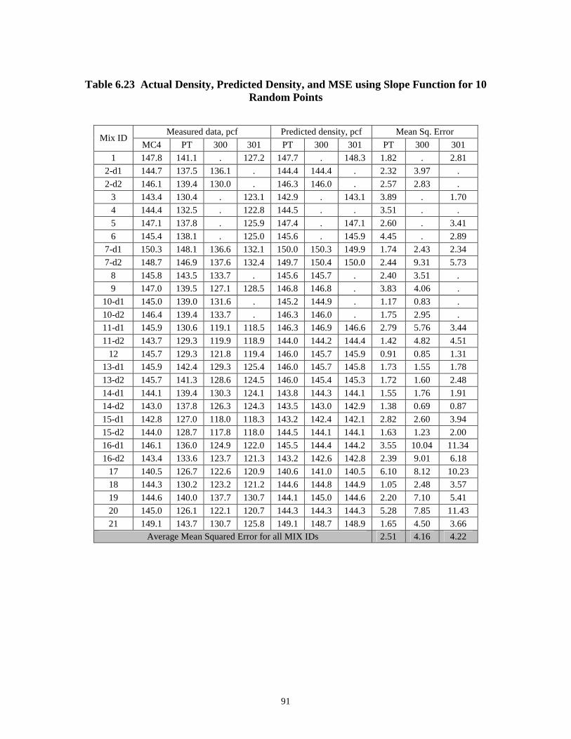
Table 6.23 Actual Density, Predicted Density, and MSE using Slope Function for 10 Random Points
Mix ID Measured data, pcf Predicted density, pcf Mean Sq. Error
MC4 PT 300 301 PT 300 301 PT 300 301
1 147.8 141.1 . 127.2 147.7 . 148.3 1.82 . 2.81
2-d1 144.7 137.5 136.1 . 144.4 144.4 . 2.32 3.97 .
2-d2 146.1 139.4 130.0 . 146.3 146.0 . 2.57 2.83 .
3 143.4 130.4 . 123.1 142.9 . 143.1 3.89 . 1.70
4 144.4 132.5 . 122.8 144.5 . . 3.51 . .
5 147.1 137.8 . 125.9 147.4 . 147.1 2.60 . 3.41
6 145.4 138.1 . 125.0 145.6 . 145.9 4.45 . 2.89
7-d1 150.3 148.1 136.6 132.1 150.0 150.3 149.9 1.74 2.43 2.34
7-d2 148.7 146.9 137.6 132.4 149.7 150.4 150.0 2.44 9.31 5.73
8 145.8 143.5 133.7 . 145.6 145.7 . 2.40 3.51 .
9 147.0 139.5 127.1 128.5 146.8 146.8 . 3.83 4.06 .
10-d1 145.0 139.0 131.6 . 145.2 144.9 . 1.17 0.83 .
10-d2 146.4 139.4 133.7 . 146.3 146.0 . 1.75 2.95 .
11-d1 145.9 130.6 119.1 118.5 146.3 146.9 146.6 2.79 5.76 3.44
11-d2 143.7 129.3 119.9 118.9 144.0 144.2 144.4 1.42 4.82 4.51
12 145.7 129.3 121.8 119.4 146.0 145.7 145.9 0.91 0.85 1.31
13-d1 145.9 142.4 129.3 125.4 146.0 145.7 145.8 1.73 1.55 1.78
13-d2 145.7 141.3 128.6 124.5 146.0 145.4 145.3 1.72 1.60 2.48
14-d1 144.1 139.4 130.3 124.1 143.8 144.3 144.1 1.55 1.76 1.91
14-d2 143.0 137.8 126.3 124.3 143.5 143.0 142.9 1.38 0.69 0.87
15-d1 142.8 127.0 118.0 118.3 143.2 142.4 142.1 2.82 2.60 3.94
15-d2 144.0 128.7 117.8 118.0 144.5 144.1 144.1 1.63 1.23 2.00
16-d1 146.1 136.0 124.9 122.0 145.5 144.4 144.2 3.55 10.04 11.34
16-d2 143.4 133.6 123.7 121.3 143.2 142.6 142.8 2.39 9.01 6.18
17 140.5 126.7 122.6 120.9 140.6 141.0 140.5 6.10 8.12 10.23
18 144.3 130.2 123.2 121.2 144.6 144.8 144.9 1.05 2.48 3.57
19 144.6 140.0 137.7 130.7 144.1 145.0 144.6 2.20 7.10 5.41
20 145.0 126.1 122.1 120.7 144.3 144.3 144.3 5.28 7.85 11.43
21 149.1 143.7 130.7 125.8 149.1 148.7 148.9 1.65 4.50 3.66 Average Mean Squared Error for all MIX IDs 2.51 4.16 4.22
91
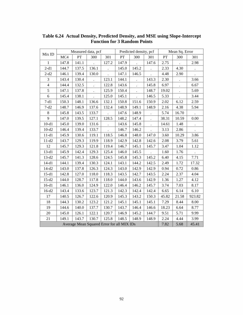
Table 6.24 Actual Density, Predicted Density, and MSE using Slope-Intercept Function for 3 Random Points
Mix ID Measured data, pcf Predicted density, pcf Mean Sq. Error
MC4 PT 300 301 PT 300 301 PT 300 301
1 147.8 141.1 . 127.2 147.9 . 147.6 2.75 . 2.98
2-d1 144.7 137.5 136.1 . 145.0 145.2 . 2.33 4.30 .
2-d2 146.1 139.4 130.0 . 147.1 146.5 . 4.48 2.90 .
3 143.4 130.4 . 123.1 144.1 . 143.3 2.30 . 3.66
4 144.4 132.5 . 122.8 143.6 . 145.8 6.97 . 6.67
5 147.1 137.8 . 125.9 150.4 . 148.7 19.02 . 5.69
6 145.4 138.1 . 125.0 145.1 . 146.5 5.33 . 3.44
7-d1 150.3 148.1 136.6 132.1 150.8 151.6 150.9 2.02 6.12 2.59
7-d2 148.7 146.9 137.6 132.4 148.9 149.1 148.9 2.16 4.38 5.94
8 145.8 143.5 133.7 . 147.6 148.9 . 5.74 16.70 .
9 147.0 139.5 127.1 128.5 148.2 147.4 . 38.31 10.59 0.00
10-d1 145.0 139.0 131.6 . 143.6 145.8 . 14.61 1.48 .
10-d2 146.4 139.4 133.7 . 146.7 146.2 . 3.13 2.86 .
11-d1 145.9 130.6 119.1 118.5 146.8 148.0 147.0 3.60 10.29 3.86
11-d2 143.7 129.3 119.9 118.9 142.9 142.8 142.6 2.08 3.79 5.61
12 145.7 129.3 121.8 119.4 146.7 145.1 145.7 3.47 1.04 1.12
13-d1 145.9 142.4 129.3 125.4 146.0 145.5 . 1.60 1.76 .
13-d2 145.7 141.3 128.6 124.5 145.8 145.3 145.2 6.40 4.15 7.71
14-d1 144.1 139.4 130.3 124.1 143.1 144.2 142.5 2.49 1.72 17.32
14-d2 143.0 137.8 126.3 124.3 143.0 142.9 142.9 0.94 0.72 0.86
15-d1 142.8 127.0 118.0 118.3 143.5 142.7 143.5 2.24 2.37 4.04
15-d2 144.0 128.7 117.8 118.0 144.0 143.6 142.9 1.36 1.27 4.12
16-d1 146.1 136.0 124.9 122.0 146.4 146.2 145.7 3.74 7.03 8.17 16-d2 143.4 133.6 123.7 121.3 142.3 142.4 142.4 6.65 6.14 6.10
17 140.5 126.7 122.6 120.9 145.3 143.2 150.3 45.82 21.58 923.82
18 144.3 130.2 123.2 121.2 145.1 145.1 145.1 7.29 8.44 8.00
19 144.6 140.0 137.7 130.7 143.7 146.4 146.6 18.23 6.64 8.77
20 145.0 126.1 122.1 120.7 146.9 145.2 144.7 9.51 5.71 9.99
21 149.1 143.7 130.7 125.8 148.5 148.9 148.9 2.24 4.44 3.99 Average Mean Squared Error for all MIX IDs 7.82 5.68 45.41
92
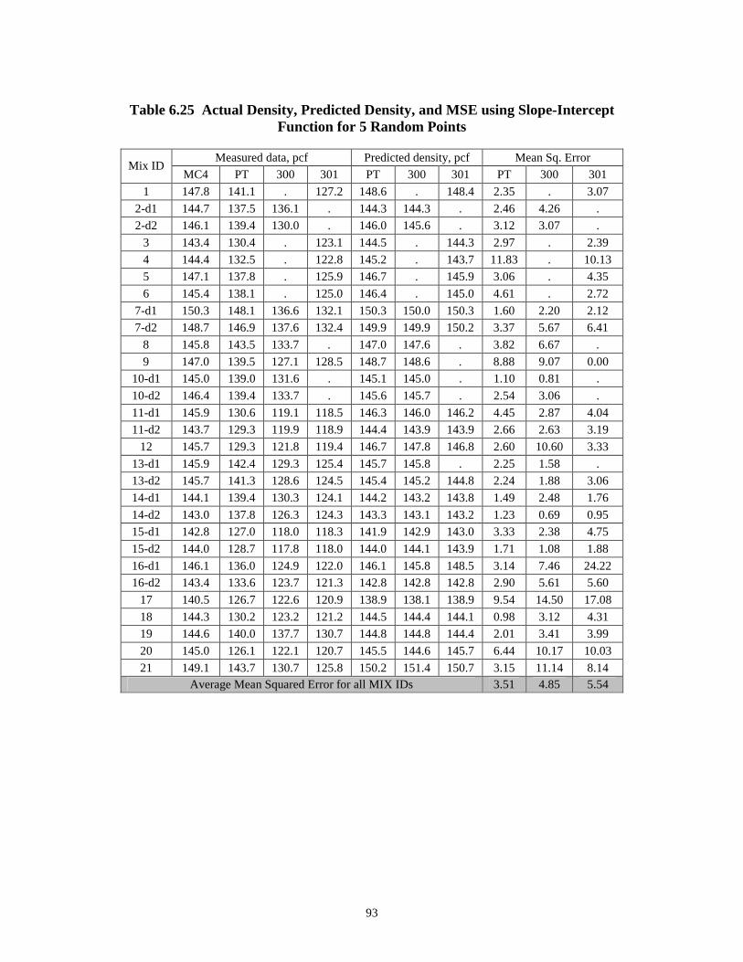
Table 6.25 Actual Density, Predicted Density, and MSE using Slope-Intercept Function for 5 Random Points
Mix ID Measured data, pcf Predicted density, pcf Mean Sq. Error
MC4 PT 300 301 PT 300 301 PT 300 301
1 147.8 141.1 . 127.2 148.6 . 148.4 2.35 . 3.07
2-d1 144.7 137.5 136.1 . 144.3 144.3 . 2.46 4.26 .
2-d2 146.1 139.4 130.0 . 146.0 145.6 . 3.12 3.07 .
3 143.4 130.4 . 123.1 144.5 . 144.3 2.97 . 2.39
4 144.4 132.5 . 122.8 145.2 . 143.7 11.83 . 10.13
5 147.1 137.8 . 125.9 146.7 . 145.9 3.06 . 4.35
6 145.4 138.1 . 125.0 146.4 . 145.0 4.61 . 2.72
7-d1 150.3 148.1 136.6 132.1 150.3 150.0 150.3 1.60 2.20 2.12
7-d2 148.7 146.9 137.6 132.4 149.9 149.9 150.2 3.37 5.67 6.41
8 145.8 143.5 133.7 . 147.0 147.6 . 3.82 6.67 .
9 147.0 139.5 127.1 128.5 148.7 148.6 . 8.88 9.07 0.00
10-d1 145.0 139.0 131.6 . 145.1 145.0 . 1.10 0.81 .
10-d2 146.4 139.4 133.7 . 145.6 145.7 . 2.54 3.06 .
11-d1 145.9 130.6 119.1 118.5 146.3 146.0 146.2 4.45 2.87 4.04
11-d2 143.7 129.3 119.9 118.9 144.4 143.9 143.9 2.66 2.63 3.19
12 145.7 129.3 121.8 119.4 146.7 147.8 146.8 2.60 10.60 3.33
13-d1 145.9 142.4 129.3 125.4 145.7 145.8 . 2.25 1.58 .
13-d2 145.7 141.3 128.6 124.5 145.4 145.2 144.8 2.24 1.88 3.06
14-d1 144.1 139.4 130.3 124.1 144.2 143.2 143.8 1.49 2.48 1.76
14-d2 143.0 137.8 126.3 124.3 143.3 143.1 143.2 1.23 0.69 0.95
15-d1 142.8 127.0 118.0 118.3 141.9 142.9 143.0 3.33 2.38 4.75
15-d2 144.0 128.7 117.8 118.0 144.0 144.1 143.9 1.71 1.08 1.88
16-d1 146.1 136.0 124.9 122.0 146.1 145.8 148.5 3.14 7.46 24.22 16-d2 143.4 133.6 123.7 121.3 142.8 142.8 142.8 2.90 5.61 5.60
17 140.5 126.7 122.6 120.9 138.9 138.1 138.9 9.54 14.50 17.08
18 144.3 130.2 123.2 121.2 144.5 144.4 144.1 0.98 3.12 4.31
19 144.6 140.0 137.7 130.7 144.8 144.8 144.4 2.01 3.41 3.99
20 145.0 126.1 122.1 120.7 145.5 144.6 145.7 6.44 10.17 10.03
21 149.1 143.7 130.7 125.8 150.2 151.4 150.7 3.15 11.14 8.14 Average Mean Squared Error for all MIX IDs 3.51 4.85 5.54
93
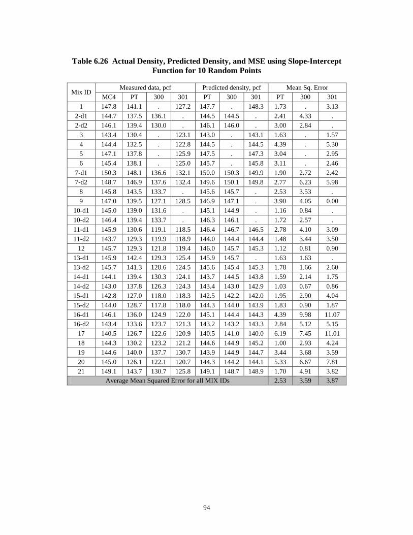
Table 6.26 Actual Density, Predicted Density, and MSE using Slope-Intercept Function for 10 Random Points
Mix ID Measured data, pcf Predicted density, pcf Mean Sq. Error
MC4 PT 300 301 PT 300 301 PT 300 301
1 147.8 141.1 . 127.2 147.7 . 148.3 1.73 . 3.13
2-d1 144.7 137.5 136.1 . 144.5 144.5 . 2.41 4.33 .
2-d2 146.1 139.4 130.0 . 146.1 146.0 . 3.00 2.84 .
3 143.4 130.4 . 123.1 143.0 . 143.1 1.63 . 1.57
4 144.4 132.5 . 122.8 144.5 . 144.5 4.39 . 5.30
5 147.1 137.8 . 125.9 147.5 . 147.3 3.04 . 2.95
6 145.4 138.1 . 125.0 145.7 . 145.8 3.11 . 2.46
7-d1 150.3 148.1 136.6 132.1 150.0 150.3 149.9 1.90 2.72 2.42
7-d2 148.7 146.9 137.6 132.4 149.6 150.1 149.8 2.77 6.23 5.98
8 145.8 143.5 133.7 . 145.6 145.7 . 2.53 3.53 .
9 147.0 139.5 127.1 128.5 146.9 147.1 . 3.90 4.05 0.00
10-d1 145.0 139.0 131.6 . 145.1 144.9 . 1.16 0.84 .
10-d2 146.4 139.4 133.7 . 146.3 146.1 . 1.72 2.57 .
11-d1 145.9 130.6 119.1 118.5 146.4 146.7 146.5 2.78 4.10 3.09
11-d2 143.7 129.3 119.9 118.9 144.0 144.4 144.4 1.48 3.44 3.50
12 145.7 129.3 121.8 119.4 146.0 145.7 145.3 1.12 0.81 0.90
13-d1 145.9 142.4 129.3 125.4 145.9 145.7 . 1.63 1.63 .
13-d2 145.7 141.3 128.6 124.5 145.6 145.4 145.3 1.78 1.66 2.60
14-d1 144.1 139.4 130.3 124.1 143.7 144.5 143.8 1.59 2.14 1.75
14-d2 143.0 137.8 126.3 124.3 143.4 143.0 142.9 1.03 0.67 0.86
15-d1 142.8 127.0 118.0 118.3 142.5 142.2 142.0 1.95 2.90 4.04
15-d2 144.0 128.7 117.8 118.0 144.3 144.0 143.9 1.83 0.90 1.87
16-d1 146.1 136.0 124.9 122.0 145.1 144.4 144.3 4.39 9.98 11.07 16-d2 143.4 133.6 123.7 121.3 143.2 143.2 143.3 2.84 5.12 5.15
17 140.5 126.7 122.6 120.9 140.5 141.0 140.0 6.19 7.45 11.01
18 144.3 130.2 123.2 121.2 144.6 144.9 145.2 1.00 2.93 4.24
19 144.6 140.0 137.7 130.7 143.9 144.9 144.7 3.44 3.68 3.59
20 145.0 126.1 122.1 120.7 144.3 144.2 144.1 5.33 6.67 7.81
21 149.1 143.7 130.7 125.8 149.1 148.7 148.9 1.70 4.91 3.82 Average Mean Squared Error for all MIX IDs 2.53 3.59 3.87
94
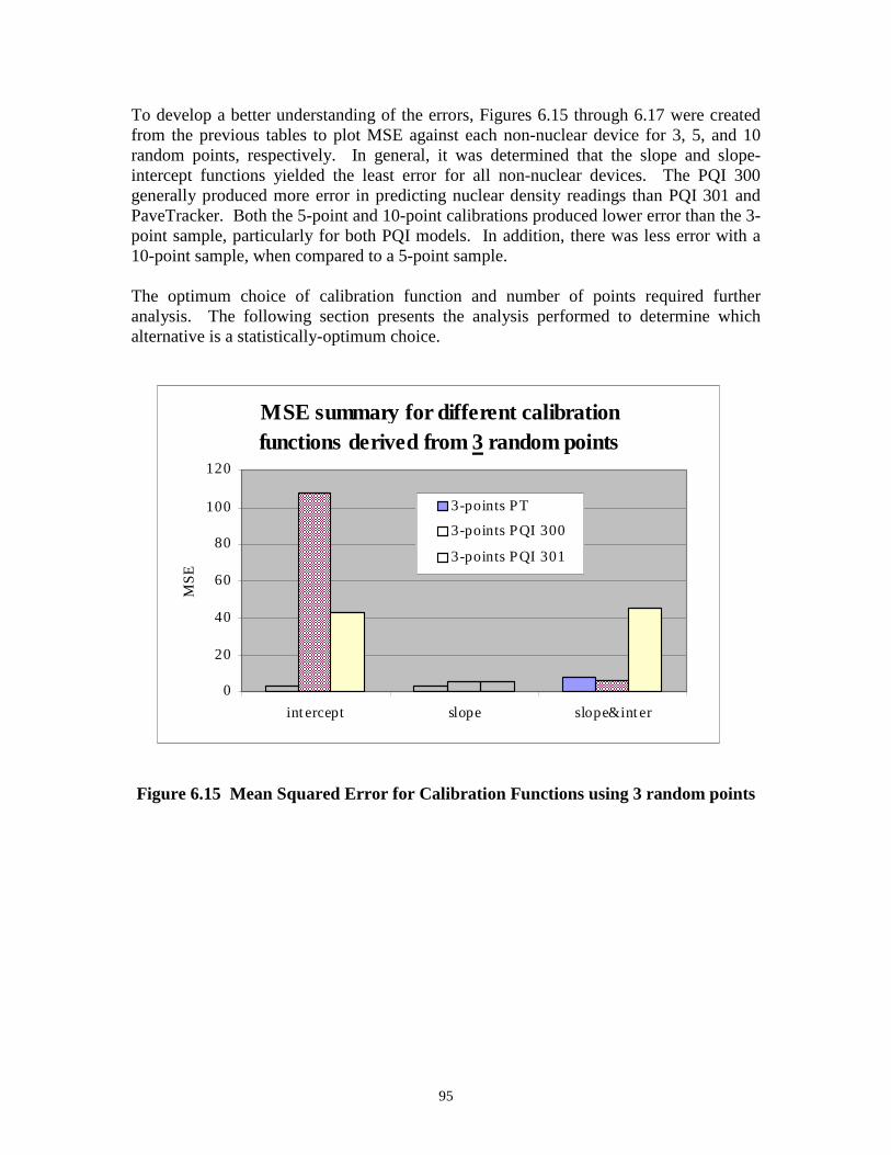
To develop a better understanding of the errors, Figures 6.15 through 6.17 were created from the previous tables to plot MSE against each non-nuclear device for 3, 5, and 10 random points, respectively. In general, it was determined that the slope and slope-intercept functions yielded the least error for all non-nuclear devices. The PQI 300 generally produced more error in predicting nuclear density readings than PQI 301 and PaveTracker. Both the 5-point and 10-point calibrations produced lower error than the 3point sample, particularly for both PQI models. In addition, there was less error with a 10-point sample, when compared to a 5-point sample.
The optimum choice of calibration function and number of points required further analysis. The following section presents the analysis performed to determine which alternative is a statistically-optimum choice.
MSE summary for different calibration functions derived from 3 random points
0
20
40
60
80
100
120
int ercept slope slope&int er
MS
E
3 -points P T
3-points P QI 300
3-points P QI 301
Figure 6.15 Mean Squared Error for Calibration Functions using 3 random points
95
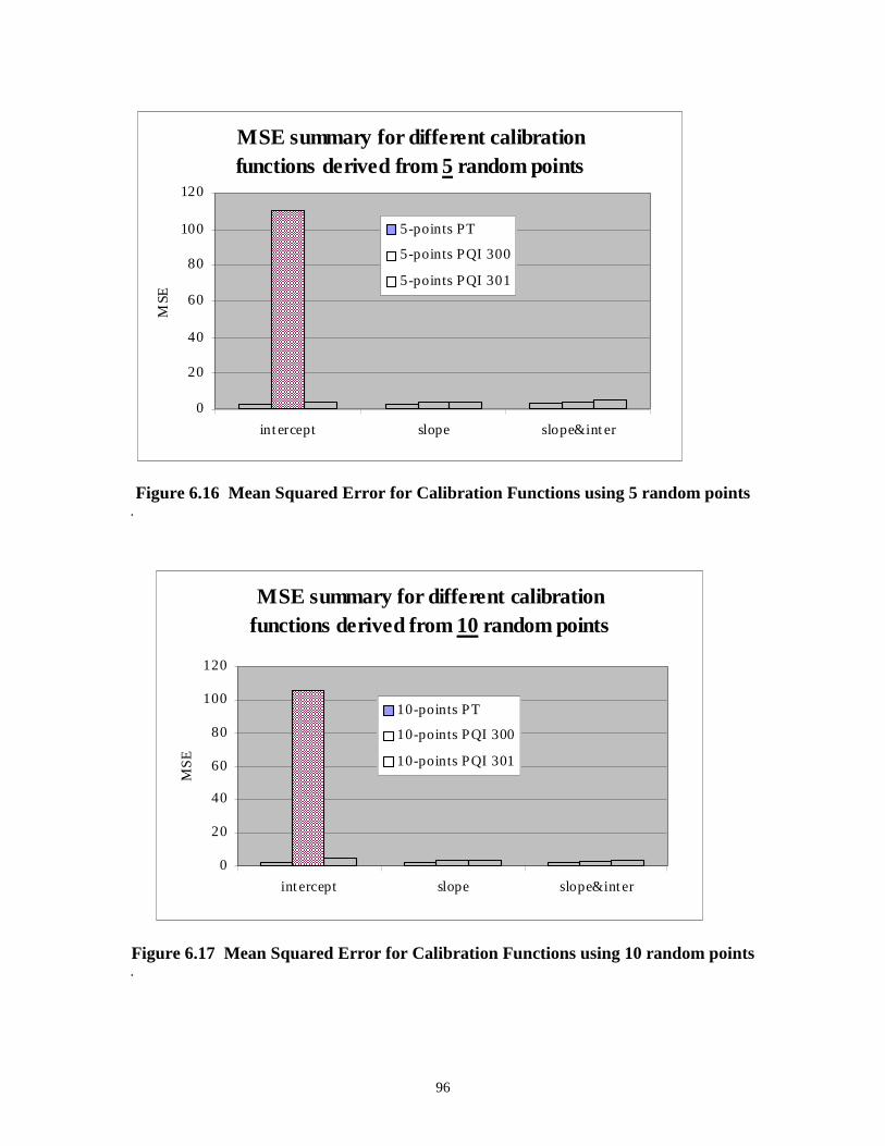
MSE summary for different calibration functions derived from 5 random points
0
20
40
60
80
100
120
int ercept slope slope&int er
MSE
5 -points PT
5-points PQI 300
5-points PQI 301
Figure 6.16 Mean Squared Error for Calibration Functions using 5 random points .
MSE summary for different calibration functions derived from 10 random points
0
20
40
60
80
100
120
int ercept slope slope&int er
MS
E
10-points PT
10-points PQI 300
10-points PQI 301
Figure 6.17 Mean Squared Error for Calibration Functions using 10 random points .
96
6.9 Statistical Verification of Calibration Functions
A statistical verification was performed across the entire data set of 21 mix IDs to assess if the actual nuclear density value was statistically close, or comparable, to that of the adjusted non-nuclear density values. The non-nuclear density values included the raw readings, and adjusted values using correction factors developed using all three calibration functions and number of random points (3, 5, and 10).
A two-sample paired t-test was the chosen function because the data sets contain a natural pairing of observations at each test site within the project. The t-test was performed at a confidence level of 95% (α = 0.05). The t-test was performed based on the null hypothesis that there was no difference between the means of the two sets. The results of t-test are presented in Table 6.27 and indicate that if the level of significance, or the p-value was greater than 0.05, the null hypothesis was accepted and that the predicted and actual density values were not statistically different.
The results show that the predictions are statistically significant only for cases when the correction factors were determined using 3 or 5 random points from the test data. The intercept function shows a good prediction with a 3-point generated correction factor. However, this case was not considered a preferred case given that this situation generated a significantly large mean-squared error in the prediction (see Table 6.18 and Figure 6.15). The key finding from this table was that the 10-point calibration for the three functions yielded insignificant differences between nuclear and adjusted non-nuclear readings.
97
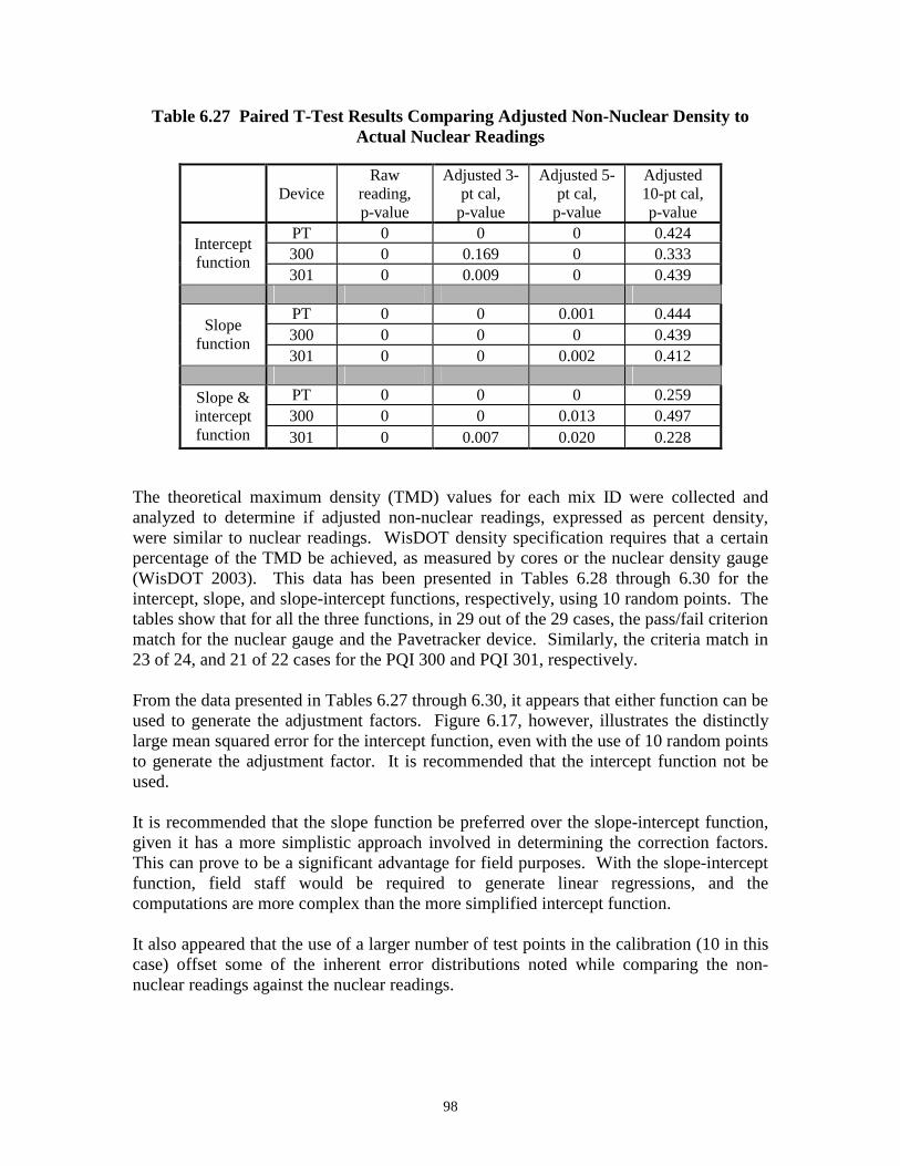
Table 6.27 Paired T-Test Results Comparing Adjusted Non-Nuclear Density to Actual Nuclear Readings
Device Raw
reading, p-value
Adjusted 3pt cal,
p-value
Adjusted 5pt cal,
p-value
Adjusted 10-pt cal, p-value
Intercept function
PT 0 0 0 0.424 300 0 0.169 0 0.333 301 0 0.009 0 0.439
Slope function
PT 0 0 0.001 0.444 300 0 0 0 0.439 301 0 0 0.002 0.412
Slope & intercept
PT 0 0 0 0.259 300 0 0 0.013 0.497
function 301 0 0.007 0.020 0.228
The theoretical maximum density (TMD) values for each mix ID were collected and analyzed to determine if adjusted non-nuclear readings, expressed as percent density, were similar to nuclear readings. WisDOT density specification requires that a certain percentage of the TMD be achieved, as measured by cores or the nuclear density gauge (WisDOT 2003). This data has been presented in Tables 6.28 through 6.30 for the intercept, slope, and slope-intercept functions, respectively, using 10 random points. The tables show that for all the three functions, in 29 out of the 29 cases, the pass/fail criterion match for the nuclear gauge and the Pavetracker device. Similarly, the criteria match in 23 of 24, and 21 of 22 cases for the PQI 300 and PQI 301, respectively.
From the data presented in Tables 6.27 through 6.30, it appears that either function can be used to generate the adjustment factors. Figure 6.17, however, illustrates the distinctly large mean squared error for the intercept function, even with the use of 10 random points to generate the adjustment factor. It is recommended that the intercept function not be used.
It is recommended that the slope function be preferred over the slope-intercept function, given it has a more simplistic approach involved in determining the correction factors. This can prove to be a significant advantage for field purposes. With the slope-intercept function, field staff would be required to generate linear regressions, and the computations are more complex than the more simplified intercept function.
It also appeared that the use of a larger number of test points in the calibration (10 in this case) offset some of the inherent error distributions noted while comparing the nonnuclear readings against the nuclear readings.
98
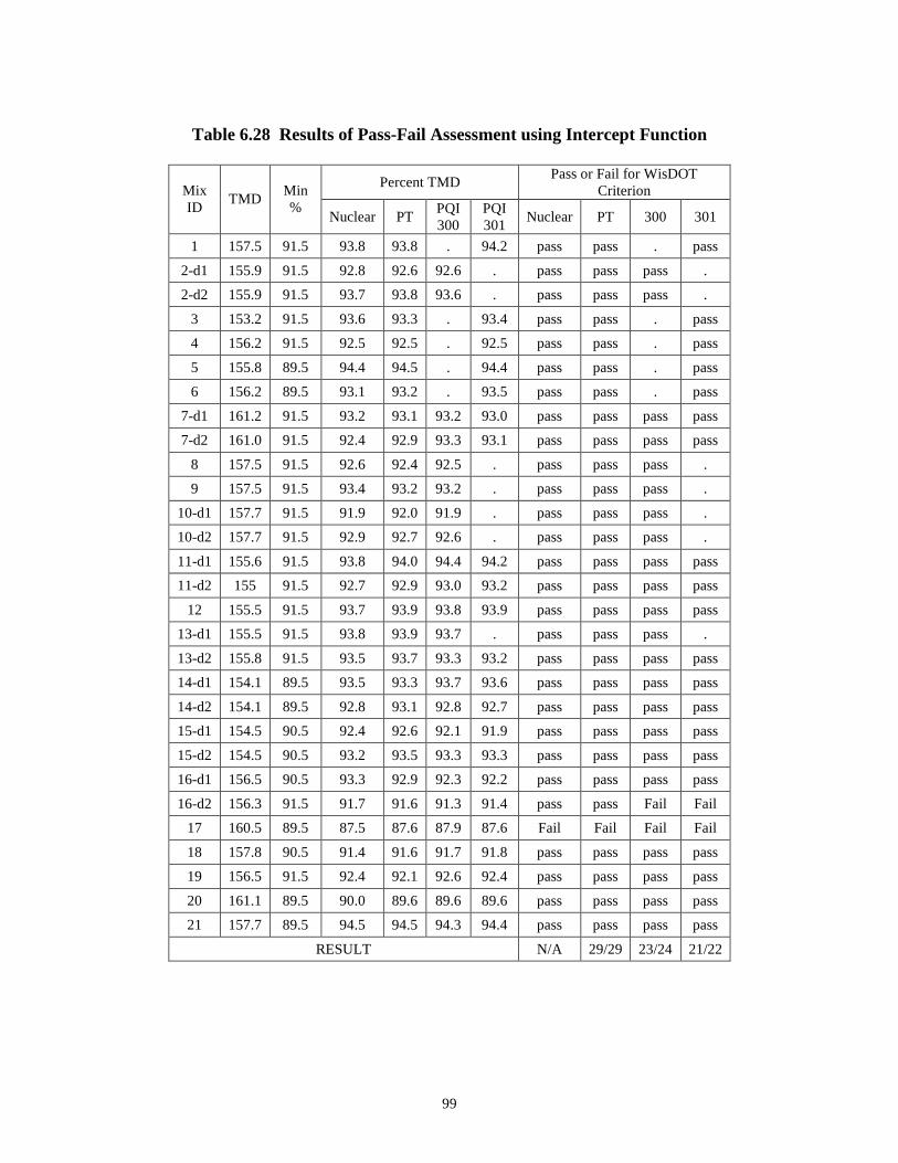
Table 6.28 Results of Pass-Fail Assessment using Intercept Function
Mix ID
TMD Min %
Percent TMD Pass or Fail for WisDOT
Criterion
Nuclear PT PQI 300
PQI 301
Nuclear PT 300 301
1 157.5 91.5 93.8 93.8 . 94.2 pass pass . pass
2-d1 155.9 91.5 92.8 92.6 92.6 . pass pass pass .
2-d2 155.9 91.5 93.7 93.8 93.6 . pass pass pass .
3 153.2 91.5 93.6 93.3 . 93.4 pass pass . pass
4 156.2 91.5 92.5 92.5 . 92.5 pass pass . pass
5 155.8 89.5 94.4 94.5 . 94.4 pass pass . pass
6 156.2 89.5 93.1 93.2 . 93.5 pass pass . pass
7-d1 161.2 91.5 93.2 93.1 93.2 93.0 pass pass pass pass
7-d2 161.0 91.5 92.4 92.9 93.3 93.1 pass pass pass pass
8 157.5 91.5 92.6 92.4 92.5 . pass pass pass .
9 157.5 91.5 93.4 93.2 93.2 . pass pass pass .
10-d1 157.7 91.5 91.9 92.0 91.9 . pass pass pass .
10-d2 157.7 91.5 92.9 92.7 92.6 . pass pass pass .
11-d1 155.6 91.5 93.8 94.0 94.4 94.2 pass pass pass pass
11-d2 155 91.5 92.7 92.9 93.0 93.2 pass pass pass pass
12 155.5 91.5 93.7 93.9 93.8 93.9 pass pass pass pass
13-d1 155.5 91.5 93.8 93.9 93.7 . pass pass pass .
13-d2 155.8 91.5 93.5 93.7 93.3 93.2 pass pass pass pass
14-d1 154.1 89.5 93.5 93.3 93.7 93.6 pass pass pass pass
14-d2 154.1 89.5 92.8 93.1 92.8 92.7 pass pass pass pass
15-d1 154.5 90.5 92.4 92.6 92.1 91.9 pass pass pass pass
15-d2 154.5 90.5 93.2 93.5 93.3 93.3 pass pass pass pass
16-d1 156.5 90.5 93.3 92.9 92.3 92.2 pass pass pass pass
16-d2 156.3 91.5 91.7 91.6 91.3 91.4 pass pass Fail Fail
17 160.5 89.5 87.5 87.6 87.9 87.6 Fail Fail Fail Fail
18 157.8 90.5 91.4 91.6 91.7 91.8 pass pass pass pass
19 156.5 91.5 92.4 92.1 92.6 92.4 pass pass pass pass
20 161.1 89.5 90.0 89.6 89.6 89.6 pass pass pass pass
21 157.7 89.5 94.5 94.5 94.3 94.4 pass pass pass pass
RESULT N/A 29/29 23/24 21/22
99
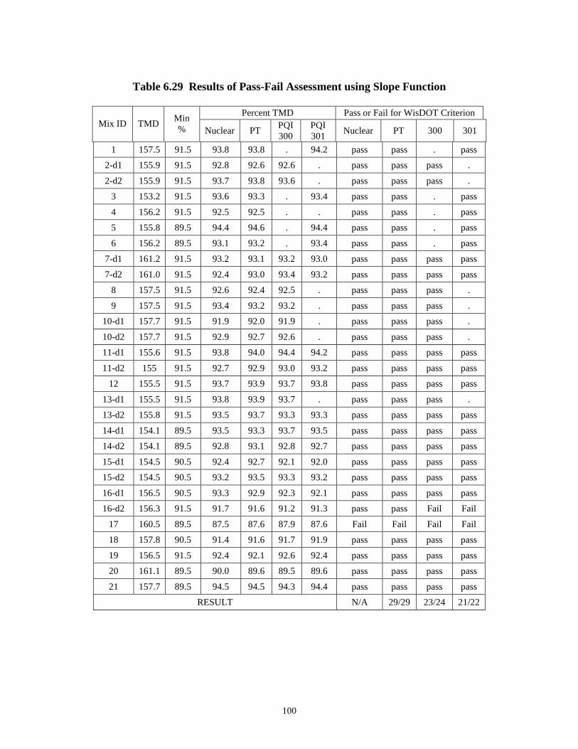
Table 6.29 Results of Pass-Fail Assessment using Slope Function
Mix ID TMD Min %
Percent TMD Pass or Fail for WisDOT Criterion
Nuclear PT PQI 300
PQI 301
Nuclear PT 300 301
1 157.5 91.5 93.8 93.8 . 94.2 pass pass . pass
2-d1 155.9 91.5 92.8 92.6 92.6 . pass pass pass .
2-d2 155.9 91.5 93.7 93.8 93.6 . pass pass pass .
3 153.2 91.5 93.6 93.3 . 93.4 pass pass . pass
4 156.2 91.5 92.5 92.5 . . pass pass . pass
5 155.8 89.5 94.4 94.6 . 94.4 pass pass . pass
6 156.2 89.5 93.1 93.2 . 93.4 pass pass . pass
7-d1 161.2 91.5 93.2 93.1 93.2 93.0 pass pass pass pass
7-d2 161.0 91.5 92.4 93.0 93.4 93.2 pass pass pass pass
8 157.5 91.5 92.6 92.4 92.5 . pass pass pass .
9 157.5 91.5 93.4 93.2 93.2 . pass pass pass .
10-d1 157.7 91.5 91.9 92.0 91.9 . pass pass pass .
10-d2 157.7 91.5 92.9 92.7 92.6 . pass pass pass .
11-d1 155.6 91.5 93.8 94.0 94.4 94.2 pass pass pass pass
11-d2 155 91.5 92.7 92.9 93.0 93.2 pass pass pass pass
12 155.5 91.5 93.7 93.9 93.7 93.8 pass pass pass pass
13-d1 155.5 91.5 93.8 93.9 93.7 . pass pass pass .
13-d2 155.8 91.5 93.5 93.7 93.3 93.3 pass pass pass pass
14-d1 154.1 89.5 93.5 93.3 93.7 93.5 pass pass pass pass
14-d2 154.1 89.5 92.8 93.1 92.8 92.7 pass pass pass pass
15-d1 154.5 90.5 92.4 92.7 92.1 92.0 pass pass pass pass
15-d2 154.5 90.5 93.2 93.5 93.3 93.2 pass pass pass pass
16-d1 156.5 90.5 93.3 92.9 92.3 92.1 pass pass pass pass
16-d2 156.3 91.5 91.7 91.6 91.2 91.3 pass pass Fail Fail
17 160.5 89.5 87.5 87.6 87.9 87.6 Fail Fail Fail Fail
18 157.8 90.5 91.4 91.6 91.7 91.9 pass pass pass pass
19 156.5 91.5 92.4 92.1 92.6 92.4 pass pass pass pass
20 161.1 89.5 90.0 89.6 89.5 89.6 pass pass pass pass
21 157.7 89.5 94.5 94.5 94.3 94.4 pass pass pass pass
RESULT N/A 29/29 23/24 21/22
100
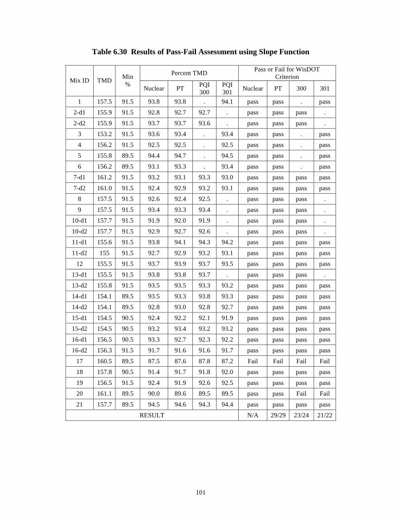
Table 6.30 Results of Pass-Fail Assessment using Slope Function
Mix ID TMD Min %
Percent TMD Pass or Fail for WisDOT
Criterion
Nuclear PT PQI 300
PQI 301
Nuclear PT 300 301
1 157.5 91.5 93.8 93.8 . 94.1 pass pass . pass
2-d1 155.9 91.5 92.8 92.7 92.7 . pass pass pass .
2-d2 155.9 91.5 93.7 93.7 93.6 . pass pass pass .
3 153.2 91.5 93.6 93.4 . 93.4 pass pass . pass
4 156.2 91.5 92.5 92.5 . 92.5 pass pass . pass
5 155.8 89.5 94.4 94.7 . 94.5 pass pass . pass
6 156.2 89.5 93.1 93.3 . 93.4 pass pass . pass
7-d1 161.2 91.5 93.2 93.1 93.3 93.0 pass pass pass pass
7-d2 161.0 91.5 92.4 92.9 93.2 93.1 pass pass pass pass
8 157.5 91.5 92.6 92.4 92.5 . pass pass pass .
9 157.5 91.5 93.4 93.3 93.4 . pass pass pass .
10-d1 157.7 91.5 91.9 92.0 91.9 . pass pass pass .
10-d2 157.7 91.5 92.9 92.7 92.6 . pass pass pass .
11-d1 155.6 91.5 93.8 94.1 94.3 94.2 pass pass pass pass
11-d2 155 91.5 92.7 92.9 93.2 93.1 pass pass pass pass
12 155.5 91.5 93.7 93.9 93.7 93.5 pass pass pass pass
13-d1 155.5 91.5 93.8 93.8 93.7 . pass pass pass .
13-d2 155.8 91.5 93.5 93.5 93.3 93.2 pass pass pass pass
14-d1 154.1 89.5 93.5 93.3 93.8 93.3 pass pass pass pass
14-d2 154.1 89.5 92.8 93.0 92.8 92.7 pass pass pass pass
15-d1 154.5 90.5 92.4 92.2 92.1 91.9 pass pass pass pass
15-d2 154.5 90.5 93.2 93.4 93.2 93.2 pass pass pass pass
16-d1 156.5 90.5 93.3 92.7 92.3 92.2 pass pass pass pass
16-d2 156.3 91.5 91.7 91.6 91.6 91.7 pass pass pass pass
17 160.5 89.5 87.5 87.6 87.8 87.2 Fail Fail Fail Fail
18 157.8 90.5 91.4 91.7 91.8 92.0 pass pass pass pass
19 156.5 91.5 92.4 91.9 92.6 92.5 pass pass pass pass
20 161.1 89.5 90.0 89.6 89.5 89.5 pass pass Fail Fail
21 157.7 89.5 94.5 94.6 94.3 94.4 pass pass pass pass
RESULT N/A 29/29 23/24 21/22
101
6.10 Stability of 10-Point Slope Function on Multiple Days Paving
Previous analysis determined that the 10-point functions produced statistically similar averages between raw nuclear and adjusted non-nuclear readings. The analysis also recommended using the 10-point slope function to adjust non-nuclear readings to the nuclear readings. In this section, the stability of the 10-point slope function was analyzed on projects where testing occurred on multiple days for the same mix ID. This analysis assessed the impact when the slope function computed from Day 1 paving was applied to Day 2 paving.
Table 6.31 presents the results, using the previous computations from Table 6.23, along with the addition of the Day 2 corrected readings using Day 1 slope function. In general, the results indicated that a Day 2 slope function used to adjust Day 2 readings was more accurate than a Day 1 slope function used to adjust Day 2 readings. This was supported by greater error values computed from the latter approach. Additionally, PaveTracker produced less error than both PQI models when the Day 1 slope function was applied to Day 2 raw readings.
When comparing the Day 2 corrected readings using the Day 2 function, and the Day 2 corrected readings using the Day 1 function, there was a change in average density. For the PaveTracker, on 7 of 8 mix IDs, the mean difference between the nuclear and adjusted non-nuclear readings increased when the Day 1 function was applied, indicating the Day 2 slope function provided a better adjustment of Day 2 readings than using the Day 1 function on Day 2. For example, on mix ID #2, the average difference increased from 0.2 pcf to 0.4 pcf, and on mix ID #15 the difference increased from 0.5 pcf to 1.3 pcf.
The PQI models produced even greater differences when the Day 1 function adjusted Day 2 non-nuclear readings. For example, on mix ID #1 using the PQI 300, the difference increased from 0.1 pcf to 8.1 pcf. Computed MSE increased from 2.8 pcf2 to 69.4 pcf2.
In summary, a daily slope function more accurately adjusts non-nuclear readings than using a previous day’s slope function. This may be the result of changes in project variables that were determined to affect non-nuclear readings. Thus, it is recommended that daily slope functions be computed until future data support a shift to using a previous day’s slope function.
102
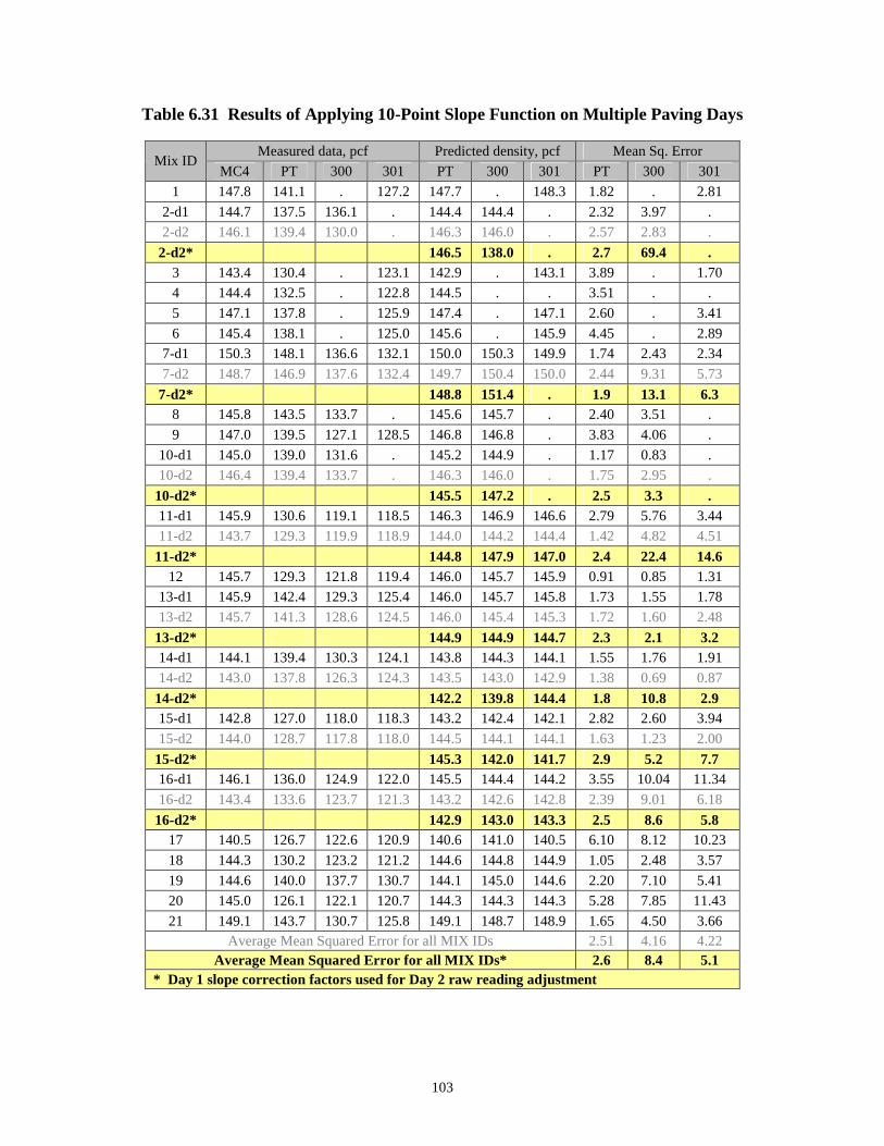
Table 6.31 Results of Applying 10-Point Slope Function on Multiple Paving Days
Mix ID Measured data, pcf Predicted density, pcf Mean Sq. Error
MC4 PT 300 301 PT 300 301 PT 300 301
1 147.8 141.1 . 127.2 147.7 . 148.3 1.82 . 2.81
2-d1 144.7 137.5 136.1 . 144.4 144.4 . 2.32 3.97 .
2-d2 146.1 139.4 130.0 . 146.3 146.0 . 2.57 2.83 .
2-d2* 146.5 138.0 . 2.7 69.4 . 3 143.4 130.4 . 123.1 142.9 . 143.1 3.89 . 1.70
4 144.4 132.5 . 122.8 144.5 . . 3.51 . .
5 147.1 137.8 . 125.9 147.4 . 147.1 2.60 . 3.41
6 145.4 138.1 . 125.0 145.6 . 145.9 4.45 . 2.89
7-d1 150.3 148.1 136.6 132.1 150.0 150.3 149.9 1.74 2.43 2.34
7-d2 148.7 146.9 137.6 132.4 149.7 150.4 150.0 2.44 9.31 5.73
7-d2* 148.8 151.4 . 1.9 13.1 6.3 8 145.8 143.5 133.7 . 145.6 145.7 . 2.40 3.51 .
9 147.0 139.5 127.1 128.5 146.8 146.8 . 3.83 4.06 .
10-d1 145.0 139.0 131.6 . 145.2 144.9 . 1.17 0.83 .
10-d2 146.4 139.4 133.7 . 146.3 146.0 . 1.75 2.95 .
10-d2* 145.5 147.2 . 2.5 3.3 . 11-d1 145.9 130.6 119.1 118.5 146.3 146.9 146.6 2.79 5.76 3.44
11-d2 143.7 129.3 119.9 118.9 144.0 144.2 144.4 1.42 4.82 4.51
11-d2* 144.8 147.9 147.0 2.4 22.4 14.6 12 145.7 129.3 121.8 119.4 146.0 145.7 145.9 0.91 0.85 1.31
13-d1 145.9 142.4 129.3 125.4 146.0 145.7 145.8 1.73 1.55 1.78
13-d2 145.7 141.3 128.6 124.5 146.0 145.4 145.3 1.72 1.60 2.48
13-d2* 144.9 144.9 144.7 2.3 2.1 3.2 14-d1 144.1 139.4 130.3 124.1 143.8 144.3 144.1 1.55 1.76 1.91
14-d2 143.0 137.8 126.3 124.3 143.5 143.0 142.9 1.38 0.69 0.87
14-d2* 142.2 139.8 144.4 1.8 10.8 2.9 15-d1 142.8 127.0 118.0 118.3 143.2 142.4 142.1 2.82 2.60 3.94
15-d2 144.0 128.7 117.8 118.0 144.5 144.1 144.1 1.63 1.23 2.00
15-d2* 145.3 142.0 141.7 2.9 5.2 7.7 16-d1 146.1 136.0 124.9 122.0 145.5 144.4 144.2 3.55 10.04 11.34
16-d2 143.4 133.6 123.7 121.3 143.2 142.6 142.8 2.39 9.01 6.18
16-d2* 142.9 143.0 143.3 2.5 8.6 5.8 17 140.5 126.7 122.6 120.9 140.6 141.0 140.5 6.10 8.12 10.23
18 144.3 130.2 123.2 121.2 144.6 144.8 144.9 1.05 2.48 3.57
19 144.6 140.0 137.7 130.7 144.1 145.0 144.6 2.20 7.10 5.41
20 145.0 126.1 122.1 120.7 144.3 144.3 144.3 5.28 7.85 11.43
21 149.1 143.7 130.7 125.8 149.1 148.7 148.9 1.65 4.50 3.66 Average Mean Squared Error for all MIX IDs 2.51 4.16 4.22
Average Mean Squared Error for all MIX IDs* 2.6 8.4 5.1 * Day 1 slope correction factors used for Day 2 raw reading adjustment
103

6.11 Investigation of Moisture Correction for PQI Models
The analysis of variance and previous plots concluded that moisture had an effect on the difference between nuclear density readings and PQI non-nuclear density readings. The previous error analysis also determined that the PQI models had a greater source of error associated with the correction to the nuclear density gauge. As a result, a moisture correction was investigated for the PQI models in an effort to manage the errors (residuals) and the difference between nuclear and non-nuclear readings.
Using pooled data from all mix types, the residual errors from the 10-point slope prediction models were plotted against moisture values. The plots for both the PQI 300 and 301 are shown in Figures 6.18 and 6.19, respectively. A least-squares regression line was fit between the residuals and moisture values and tested for significance. From this test, along with a visual analysis of the least-squares regression line, there was no correlation between the residuals and moisture values, indicating that no valid correction factor can be introduced for moisture in the pavement.
10
8
6
4 y = 0.1368x - 0.5887
R2 = 0.0196 2
0
0 2 4 6 8 10 12 -2
-4
-6
-8
PQI 300 residual data -10 Linear (PQI 300 residual data)
-12
Moisture Content - PQI 300
Figure 6.18 Moisture Correction for PQI 300 using Pooled Data
Res
idua
l Err
or fr
om P
QI
300
104
14
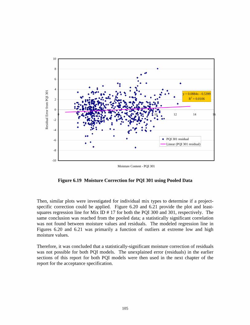
Res
idua
l Err
or f
rom
PQ
I 30
1
10
8
6
4
y = 0.0884x - 0.5399
R2 = 0.0106 2
0
0 2 4 6 8 10 12 14
-2
-4
PQI 301 residual -6 Linear (PQI 301 residual)
-8
-10
Moisture Content - PQI 301
Figure 6.19 Moisture Correction for PQI 301 using Pooled Data
Then, similar plots were investigated for individual mix types to determine if a project-specific correction could be applied. Figure 6.20 and 6.21 provide the plot and least-squares regression line for Mix ID # 17 for both the PQI 300 and 301, respectively. The same conclusion was reached from the pooled data; a statistically significant correlation was not found between moisture values and residuals. The modeled regression line in Figures 6.20 and 6.21 was primarily a function of outliers at extreme low and high moisture values.
Therefore, it was concluded that a statistically-significant moisture correction of residuals was not possible for both PQI models. The unexplained error (residuals) in the earlier sections of this report for both PQI models were then used in the next chapter of the report for the acceptance specification.
105
16
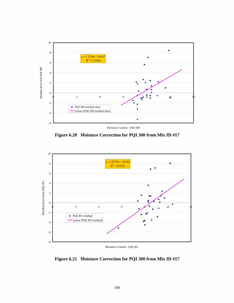
y = 1.3724x - 10.417
R2 = 0.1658
-6
-4
-2
0
2
4
6
8
10
0 2 4 6 8 10 12 Res
idua
l Err
or f
rom
PQ
I 30
0
PQI 300 residual data
Linear (PQI 300 residual data)
Moisture Content - PQI 300
Figure 6.20 Moisture Correction for PQI 300 from Mix ID #17
y = 1.6776x - 14.242
R2 = 0.2255
-8
-6
-4
-2
0
2
4
6
8
10
0 2 4 6 8 10 12
Res
idua
l Err
or f
rom
PQ
I 30
1
PQI 301 residual
Linear (PQI 301 residual)
Moisture Content - PQI 301
Figure 6.21 Moisture Correction for PQI 300 from Mix ID #17
106
CHAPTER 7 NON-NUCLEAR QC/QA ANALYSIS
7.1 Introduction
This chapter investigated the application of the non-nuclear calibration procedure for quality control and acceptance testing on WisDOT projects. The investigation used the current WisDOT Section 460 specification as a starting basis. First, the current nuclear density specification was investigated, then the new test procedure for non-nuclear gauges was developed. Finally, a procedure for determining the allowable difference between non-nuclear density gauges was outlined.
7.2 Current WisDOT Specification
Currently, WisDOT computes the mean to determine specification compliance for pavement density. Seven nuclear density readings are randomly taken within a 750-ton lot, averaged, and compared against specification limits to determine contractor compliance and payment (WisDOT 2003). The sample size of n=7 was selected by WisDOT after the conclusion of the 1996 density study.
7.2.1 Previous Density Study
From the previous density study, an equation was proposed that incorporated the mat variability, as measured by cores, and a regression equation from 14 projects that corrected the nuclear readings to the core value (Hanna et al. 1996). It was learned during the study that the nuclear density gauge read higher than cores for lower maximum density values (say, 145 pcf), and lower than cores for higher maximum density values (say, 160 pcf). Thus, correction of nuclear readings to core density was recommended with a regression equation. Equation 7.1 was proposed to determine the number of samples per lot. [Note – Equation 7.1 in this report was Equation 4.3 in the 1996 report.]
σ 2 + σ 2 mat Equation .3.6
C.I. = Z ..................................................................(7.1) n
Where: C.I. = confidence interval; Z = z-statistic for desired level of confidence; σmat
2 = variance of mat (standard deviation of mat squared); σEquation 3.6
2 = mean square error of regression equation; and n = number of density samples per lot.
A 95% confidence level (5% risk level) and confidence interval of ± 1.0 pcf were specified for the estimated density average (Hanna et al. 1996). Using data from 14
107
projects, the population mat variance was estimated to be 4.0 pcf2, and the resultant population standard deviation estimate was 2.0 pcf. The error in Equation 3.6, as estimated by the Mean Square Error term during traditional least squares regression, was 2.3 pcf2.
Table 7.1 illustrates the use of Equation 7.1 and the relationship of sample size with confidence limits, using the following values from the 1996 report: Z = 1.96; σmat
2 = 4.0 pcf2; and σEquation 3.6
2 = 2.3 pcf2. In the last column, a confidence interval of percent density is provided for a theoretical maximum density of 158 pcf to put the interval in context of normal field use.
Table 7.1 Relationship of Confidence Interval and Number of Tests (Adopted from Hanna et al. 1996)
Sample Size,
n (1)
Confidence Interval, +/- pcf
(2)
Confidence Intervala ,
+/- % (3)
1 4.9 3.1 2 3.5 2.2 3 2.8 1.8 4 2.5 1.6 5 2.2 1.4 6 2.0 1.3 7 1.9 1.2 8 1.7 1.1 9 1.6 1.0
10 1.6 1.0 11 1.5 0.9 12 1.4 0.9 13 1.4 0.9 14 1.3 0.8 15 1.3 0.8 16 1.2 0.8 17 1.2 0.8 18 1.2 0.7 19 1.1 0.7 20 1.1 0.7 21 1.1 0.7 22 1.0 0.7 23 1.0 0.6 24 1.0 0.6 25 1.0 0.6
a Interval based on 158 pcf maximum density
108
Clearly, the confidence interval narrowed as the number of samples was increased. Beginning at a sample size of n=22, the confidence interval was at the desired width of ± 1.0 pcf (after rounding). Thus, the 1996 density study recommended a total of 25 density tests to estimate the average pavement density within ± 1.0 pcf when both the mat variability and regression equation error were considered (Hanna et al. 1996).
The 1996 study also recommended that two 1-minute nuclear readings be taken consecutively at each test site and compared so that the difference did not exceed 1.0 pcf. Then, the two readings were to be averaged to produce a single density reading for the test site. Two 1-minute readings had the advantage of detecting testing error by comparing reading differences, and two 1-minute readings were able to estimate the same mean density as a single 4-minute test. Another benefit was testing time, where two 1minute tests required half the test time of a single 4-minute test.
After conclusion of the 1996 study, WisDOT elected not to use the regression equation, the average of two 1-minute nuclear readings per test site, and n=25 test sites per lot. Rather, a single 4-minute nuclear reading was selected, and the average of n=7 test sites were used to determine pavement density within a 750-ton lot (WisDOT 2003). Cores were not used to calibrate the nuclear gauge on the traditional mixes (LV, MV, and HV), however, cores were specified with SMA-type mixes. Nuclear gauge calibration was determined on each project by comparing the mean difference of two (or more) gauges at 10 correlation test sites. If the mean difference was within 1.0 pcf, the gauges were approved for use on the project. If the mean difference was exceeded, an investigation was conducted, and possibly the gauge out of calibration was disqualified from the project.
7.2.2 Analysis of Current Specification
A sample size of n=25 test sites with two 1-minute readings density readings would have required a significant testing effort by field staff for each 750-ton lot (approximately one hour of testing time, plus 40 to 50 minutes for layout and travel between sites). However, the implications of the current n=7 sample size, and payment tolerance of 0.5% required investigation as new data were collected in this study, and WisDOT and industry transition towards non-nuclear density devices.
Since only the mat variability was considered in the current specification, Equation 7.1 was modified by removing the regression error component to yield Equation 7.2. Similar to Equation 7.1, Equation 7.2 has four inter-related components, including: (1) confidence limits of the mean, (2) Z-statistic for the probability level, (3) variability as measured by the population standard deviation or variance, and (4) number of samples. As Equations 7.2 implies, there is a lesser number of samples required when the precision is reduced, when the probability level is reduced, or when the standard deviation is small.
109
C.I.= ± Z * n
σ .......................................................................................(7.2)
Where: C.I. = confidence interval; Z = z-statistic for desired level of confidence; σ = standard deviation of the mat; and n = number of samples. .
Data from the 16 projects (21 mix types) in this study found that the mat population standard deviation generated from 20 to 30 test sites ranged from 1.1 pcf to 4.0 pcf. It was not possible to estimate the population standard deviation value for every 750-ton lot in the study because of several factors, such the movement of traffic control on projects constructed under traffic, time for coring, waiting for rollers to clear, and only testing the standard n=7 test sites with the QC project gauge.
From the 1996 study, and 2005 data in this study, a median value for mat standard deviation was specified at 2.0 pcf. Table 7.2 shows the relationship of sample size with confidence limits using Equation 7.2 and the following input values: Z = 1.96 and σmat = 2.0 pcf. The last column calculated a confidence interval of percent density using a typical theoretical maximum density of 158 pcf (Gmm = 2.539) to put the interval in field context.
Calculations in Table 7.2 indicate that the current n=7 sample size, coupled with a 95% probability level (5% risk) and mat standard deviation of 2.0 pcf, yielded a confidence interval of ± 1.5 pcf, and ± 0.9 % density. This indicates that both WisDOT and contractors are exposing themselves to greater risk than the recommended 5% level. The current specification begins penalizing contractors at 0.5% less than the specified minimum density value (i.e., 92% minimum density begins penalties at 91.5% actual density). The current n=7 sample size allows the mean interval to encroach 0.4% density beyond that penalty threshold (0.9% - 0.5% = 0.4%). Additionally, the wider interval allows a greater probability of achieving a density bonus incentive.
Based on a sample size of n=7 and mat standard deviation of 2.0 pcf, the probability level of the finding the average density within ± 1.0 pcf was estimated to be 81.4% (z=1.323). The probability level of the finding the average within ± 0.5 % density using TMD=158 pcf was 70.4% (z=1.045). It is recommended that adjustments be made to the current nuclear density specification if risk levels are to be reduced from current levels of about 20% for the pcf average, and 30% for the percent density average. The sample size should be increased and/or the penalty tolerance be increased.
110
Table 7.2 Current Relationship of Confidence Interval and Number of Tests
Sample Size,
n (1)
Confidence Interval, +/- pcf
(2)
Confidence Intervala ,
+/- % (3)
1 3.9 2.5 2 2.8 1.8 3 2.3 1.4 4 2.0 1.2 5 1.8 1.1 6 1.6 1.0 7 1.5 0.9 8 1.4 0.9 9 1.3 0.8
10 1.2 0.8 11 1.2 0.7 12 1.1 0.7 13 1.1 0.7 14 1.0 0.7 15 1.0 0.6 16 1.0 0.6 17 1.0 0.6 18 0.9 0.6 19 0.9 0.6 20 0.9 0.6 21 0.9 0.5 22 0.8 0.5 23 0.8 0.5 24 0.8 0.5 25 0.8 0.5
a Interval based on 158 pcf maximum density
111
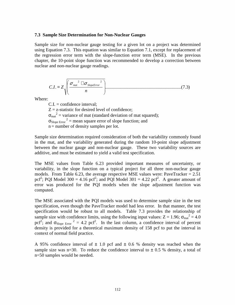
7.3 Sample Size Determination for Non-Nuclear Gauges
Sample size for non-nuclear gauge testing for a given lot on a project was determined using Equation 7.3. This equation was similar to Equation 7.1, except for replacement of the regression error term with the slope-function error term (MSE). In the previous chapter, the 10-point slope function was recommended to develop a correction between nuclear and non-nuclear gauge readings.
σ 2 +σ 2 mat SlopeError
C.I . = Z ..................................................................(7.3) n
Where: C.I. = confidence interval; Z = z-statistic for desired level of confidence; σmat
2 = variance of mat (standard deviation of mat squared); σSlope Error
2 = mean square error of slope function; and n = number of density samples per lot.
Sample size determination required consideration of both the variability commonly found in the mat, and the variability generated during the random 10-point slope adjustment between the nuclear gauge and non-nuclear gauge. These two variability sources are additive, and must be estimated to yield a valid test specification.
The MSE values from Table 6.23 provided important measures of uncertainty, or variability, in the slope function on a typical project for all three non-nuclear gauge models. From Table 6.23, the average respective MSE values were: PaveTracker = 2.51 pcf2; PQI Model 300 = 4.16 pcf2; and PQI Model 301 = 4.22 pcf2. A greater amount of error was produced for the PQI models when the slope adjustment function was computed.
The MSE associated with the PQI models was used to determine sample size in the test specification, even though the PaveTracker model had less error. In that manner, the test specification would be robust to all models. Table 7.3 provides the relationship of sample size with confidence limits, using the following input values: Z = 1.96; σmat
2 = 4.0 pcf2; and σSlope Error
2 = 4.2 pcf2. In the last column, a confidence interval of percent density is provided for a theoretical maximum density of 158 pcf to put the interval in context of normal field practice.
A 95% confidence interval of ± 1.0 pcf and ± 0.6 % density was reached when the sample size was n=30. To reduce the confidence interval to ± 0.5 % density, a total of n=50 samples would be needed.
112
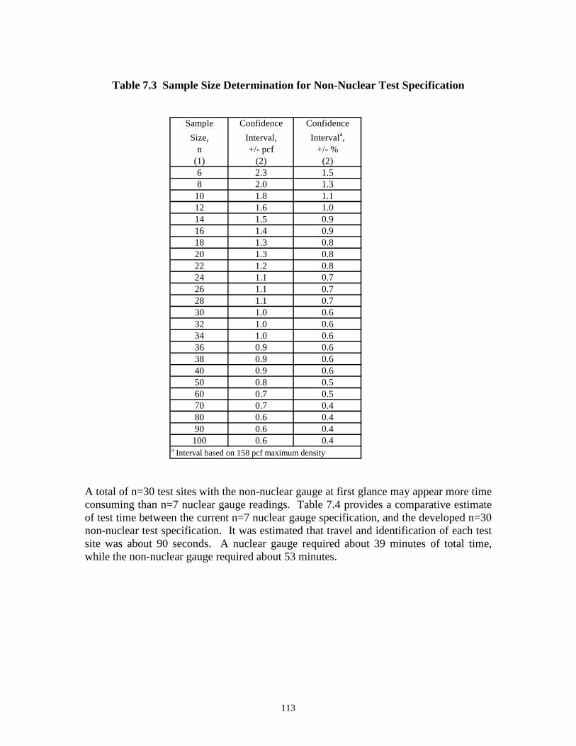
Table 7.3 Sample Size Determination for Non-Nuclear Test Specification
Sample
Size, n
(1)
Confidence
Interval, +/- pcf
(2)
Confidence
Intervala , +/- %
(2) 6 2.3 1.5 8 2.0 1.3
10 1.8 1.1 12 1.6 1.0 14 1.5 0.9 16 1.4 0.9 18 1.3 0.8 20 1.3 0.8 22 1.2 0.8 24 1.1 0.7 26 1.1 0.7 28 1.1 0.7 30 1.0 0.6 32 1.0 0.6 34 1.0 0.6 36 0.9 0.6 38 0.9 0.6 40 0.9 0.6 50 0.8 0.5 60 0.7 0.5 70 0.7 0.4 80 0.6 0.4 90 0.6 0.4
100 0.6 0.4 a Interval based on 158 pcf maximum density
A total of n=30 test sites with the non-nuclear gauge at first glance may appear more time consuming than n=7 nuclear gauge readings. Table 7.4 provides a comparative estimate of test time between the current n=7 nuclear gauge specification, and the developed n=30 non-nuclear test specification. It was estimated that travel and identification of each test site was about 90 seconds. A nuclear gauge required about 39 minutes of total time, while the non-nuclear gauge required about 53 minutes.
113
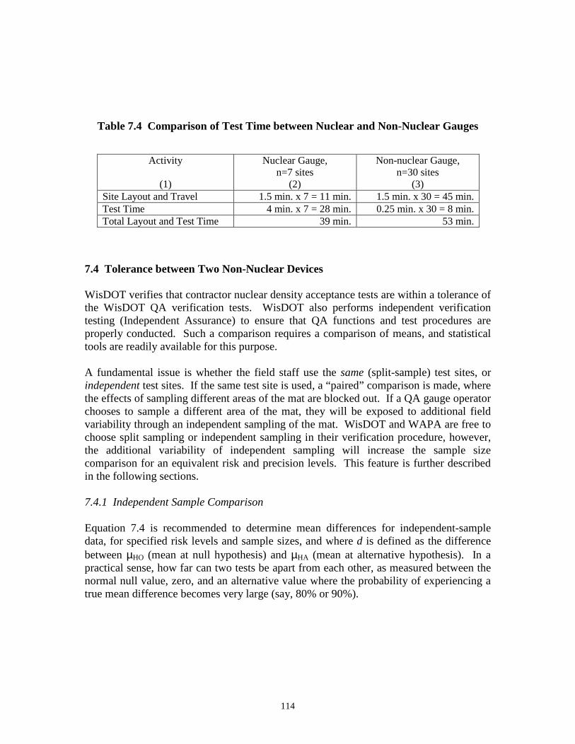
Table 7.4 Comparison of Test Time between Nuclear and Non-Nuclear Gauges
Activity
(1)
Nuclear Gauge, n=7 sites
(2)
Non-nuclear Gauge, n=30 sites
(3) Site Layout and Travel 1.5 min. x 7 = 11 min. 1.5 min. x 30 = 45 min. Test Time 4 min. x 7 = 28 min. 0.25 min. x 30 = 8 min. Total Layout and Test Time 39 min. 53 min.
7.4 Tolerance between Two Non-Nuclear Devices
WisDOT verifies that contractor nuclear density acceptance tests are within a tolerance of the WisDOT QA verification tests. WisDOT also performs independent verification testing (Independent Assurance) to ensure that QA functions and test procedures are properly conducted. Such a comparison requires a comparison of means, and statistical tools are readily available for this purpose.
A fundamental issue is whether the field staff use the same (split-sample) test sites, or independent test sites. If the same test site is used, a “paired” comparison is made, where the effects of sampling different areas of the mat are blocked out. If a QA gauge operator chooses to sample a different area of the mat, they will be exposed to additional field variability through an independent sampling of the mat. WisDOT and WAPA are free to choose split sampling or independent sampling in their verification procedure, however, the additional variability of independent sampling will increase the sample size comparison for an equivalent risk and precision levels. This feature is further described in the following sections.
7.4.1 Independent Sample Comparison
Equation 7.4 is recommended to determine mean differences for independent-sample data, for specified risk levels and sample sizes, and where d is defined as the difference between µHO (mean at null hypothesis) and µHA (mean at alternative hypothesis). In a practical sense, how far can two tests be apart from each other, as measured between the normal null value, zero, and an alternative value where the probability of experiencing a true mean difference becomes very large (say, 80% or 90%).
114
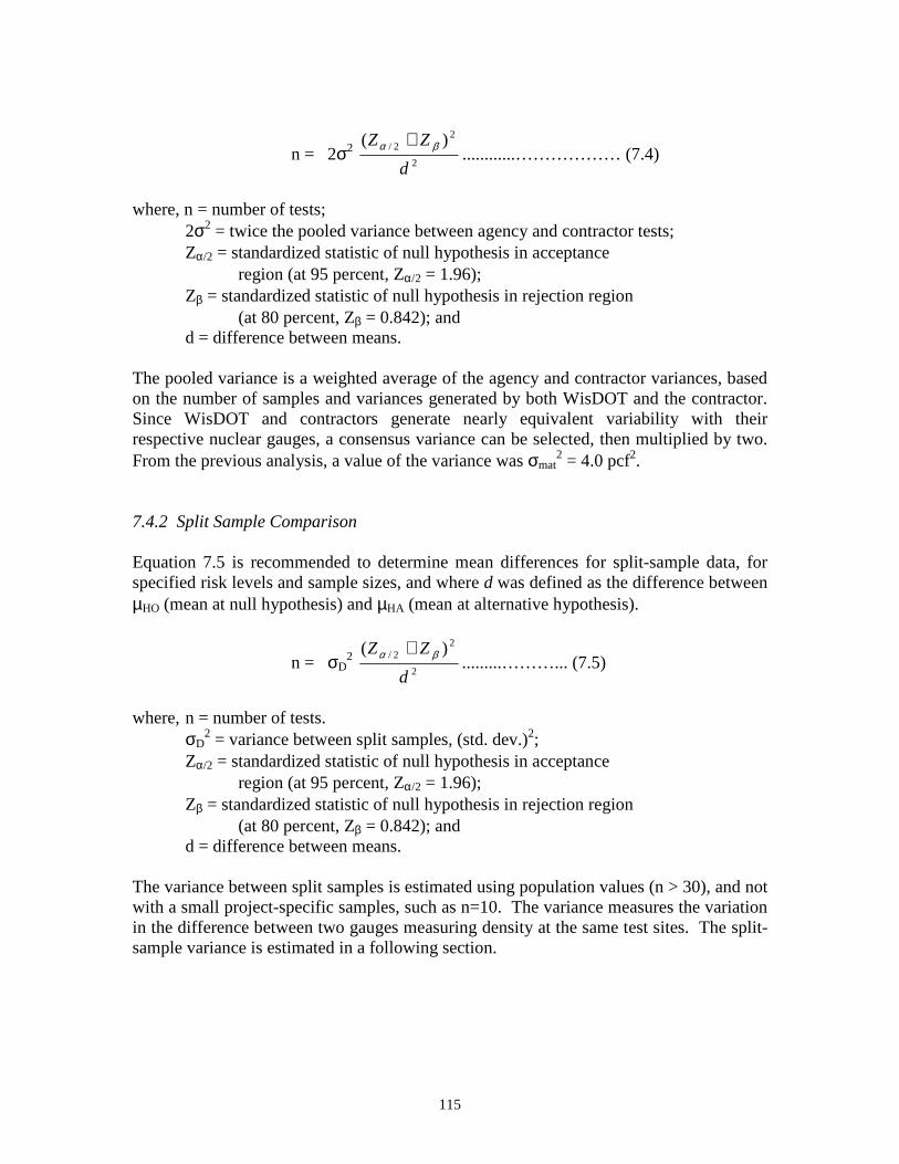
(Z + Z ) 2 α / 2 β
n = 2σ2 2
............……………… (7.4) d
where, n = number of tests; 2σ2 = twice the pooled variance between agency and contractor tests; Zα/2 = standardized statistic of null hypothesis in acceptance
region (at 95 percent, Zα/2 = 1.96); Zβ = standardized statistic of null hypothesis in rejection region
(at 80 percent, Zβ = 0.842); and d = difference between means.
The pooled variance is a weighted average of the agency and contractor variances, based on the number of samples and variances generated by both WisDOT and the contractor. Since WisDOT and contractors generate nearly equivalent variability with their respective nuclear gauges, a consensus variance can be selected, then multiplied by two. From the previous analysis, a value of the variance was σmat
2 = 4.0 pcf2.
7.4.2 Split Sample Comparison
Equation 7.5 is recommended to determine mean differences for split-sample data, for specified risk levels and sample sizes, and where d was defined as the difference between µHO (mean at null hypothesis) and µHA (mean at alternative hypothesis).
(Zα / 2 + Z β )2
n = σD2 .........………... (7.5)
d 2
where, n = number of tests. σD
2 = variance between split samples, (std. dev.)2; Zα/2 = standardized statistic of null hypothesis in acceptance
region (at 95 percent, Zα/2 = 1.96); Zβ = standardized statistic of null hypothesis in rejection region
(at 80 percent, Zβ = 0.842); and d = difference between means.
The variance between split samples is estimated using population values (n > 30), and not with a small project-specific samples, such as n=10. The variance measures the variation in the difference between two gauges measuring density at the same test sites. The split-sample variance is estimated in a following section.
115
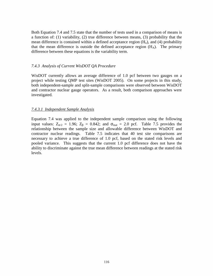
Both Equation 7.4 and 7.5 state that the number of tests used in a comparison of means is a function of: (1) variability, (2) true difference between means, (3) probability that the mean difference is contained within a defined acceptance region (Ho), and (4) probability that the mean difference is outside the defined acceptance region (HA). The primary difference between these equations is the variability term.
7.4.3 Analysis of Current WisDOT QA Procedure
WisDOT currently allows an average difference of 1.0 pcf between two gauges on a project while testing QMP test sites (WisDOT 2005). On some projects in this study, both independent-sample and split-sample comparisons were observed between WisDOT and contractor nuclear gauge operators. As a result, both comparison approaches were investigated.
7.4.3.1 Independent Sample Analysis
Equation 7.4 was applied to the independent sample comparison using the following input values: Zα/2 = 1.96; Zβ = 0.842; and σmat = 2.0 pcf. Table 7.5 provides the relationship between the sample size and allowable difference between WisDOT and contractor nuclear readings. Table 7.5 indicates that 40 test site comparisons are necessary to achieve a true difference of 1.0 pcf, based on the stated risk levels and pooled variance. This suggests that the current 1.0 pcf difference does not have the ability to discriminate against the true mean difference between readings at the stated risk levels.
116
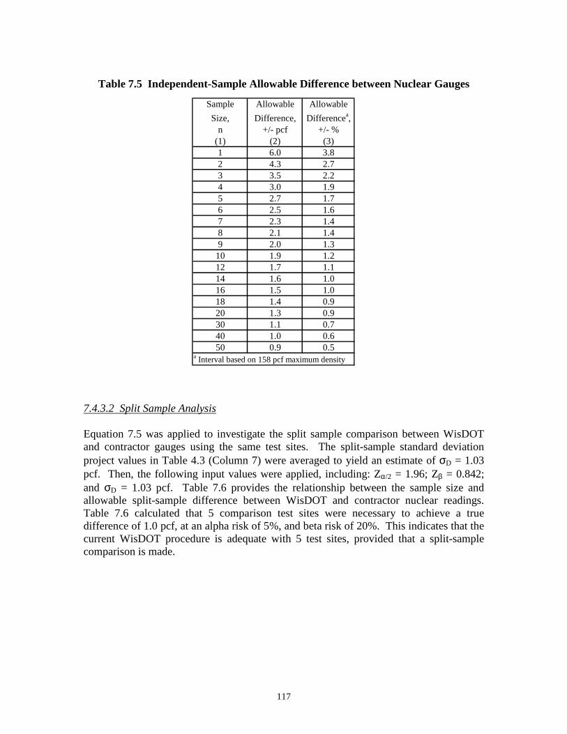
Table 7.5 Independent-Sample Allowable Difference between Nuclear Gauges
Sample
Size, n
(1)
Allowable
Difference, +/- pcf
(2)
Allowable
Differencea , +/- %
(3) 1 6.0 3.8 2 4.3 2.7 3 3.5 2.2 4 3.0 1.9 5 2.7 1.7 6 2.5 1.6 7 2.3 1.4 8 2.1 1.4 9 2.0 1.3
10 1.9 1.2 12 1.7 1.1 14 1.6 1.0 16 1.5 1.0 18 1.4 0.9 20 1.3 0.9 30 1.1 0.7 40 1.0 0.6 50 0.9 0.5
a Interval based on 158 pcf maximum density
7.4.3.2 Split Sample Analysis
Equation 7.5 was applied to investigate the split sample comparison between WisDOT and contractor gauges using the same test sites. The split-sample standard deviation project values in Table 4.3 (Column 7) were averaged to yield an estimate of σD = 1.03 pcf. Then, the following input values were applied, including: Zα/2 = 1.96; Zβ = 0.842; and σD = 1.03 pcf. Table 7.6 provides the relationship between the sample size and allowable split-sample difference between WisDOT and contractor nuclear readings. Table 7.6 calculated that 5 comparison test sites were necessary to achieve a true difference of 1.0 pcf, at an alpha risk of 5%, and beta risk of 20%. This indicates that the current WisDOT procedure is adequate with 5 test sites, provided that a split-sample comparison is made.
117
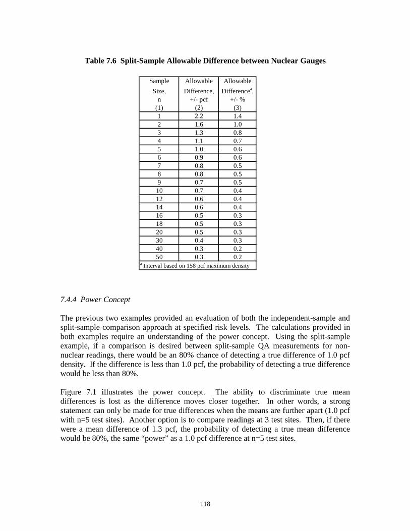
Table 7.6 Split-Sample Allowable Difference between Nuclear Gauges
Sample
Size, n
(1)
Allowable
Difference, +/- pcf
(2)
Allowable
Differencea , +/- %
(3) 1 2.2 1.4 2 1.6 1.0 3 1.3 0.8 4 1.1 0.7 5 1.0 0.6 6 0.9 0.6 7 0.8 0.5 8 0.8 0.5 9 0.7 0.5
10 0.7 0.4 12 0.6 0.4 14 0.6 0.4 16 0.5 0.3 18 0.5 0.3 20 0.5 0.3 30 0.4 0.3 40 0.3 0.2 50 0.3 0.2
a Interval based on 158 pcf maximum density
7.4.4 Power Concept
The previous two examples provided an evaluation of both the independent-sample and split-sample comparison approach at specified risk levels. The calculations provided in both examples require an understanding of the power concept. Using the split-sample example, if a comparison is desired between split-sample QA measurements for nonnuclear readings, there would be an 80% chance of detecting a true difference of 1.0 pcf density. If the difference is less than 1.0 pcf, the probability of detecting a true difference would be less than 80%.
Figure 7.1 illustrates the power concept. The ability to discriminate true mean differences is lost as the difference moves closer together. In other words, a strong statement can only be made for true differences when the means are further apart (1.0 pcf with n=5 test sites). Another option is to compare readings at 3 test sites. Then, if there were a mean difference of 1.3 pcf, the probability of detecting a true mean difference would be 80%, the same “power” as a 1.0 pcf difference at n=5 test sites.
118
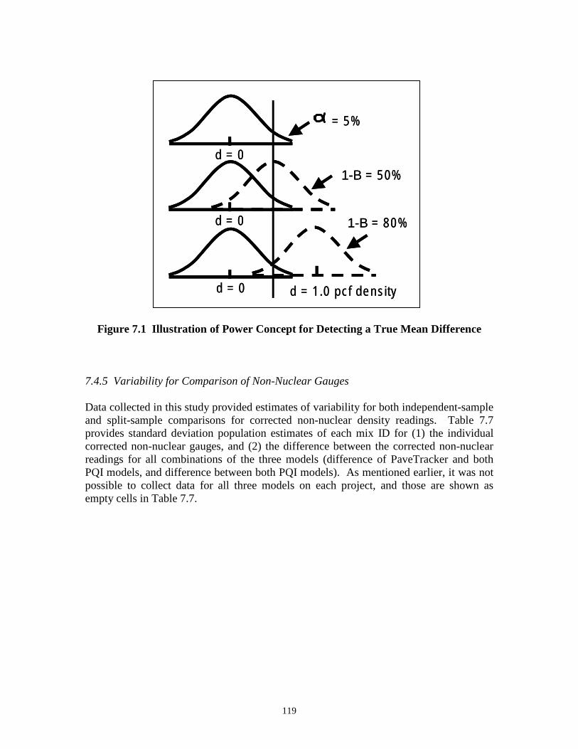
d = 0
d = 0
d = 0
= 5%
1-B = 50%
1-B = 80%
d = 1.0 pcf density
d = 0
d = 0
d = 0
= 5%
1-B = 50%
1-B = 80%
d = 1.0 pcf density
Figure 7.1 Illustration of Power Concept for Detecting a True Mean Difference
7.4.5 Variability for Comparison of Non-Nuclear Gauges
Data collected in this study provided estimates of variability for both independent-sample and split-sample comparisons for corrected non-nuclear density readings. Table 7.7 provides standard deviation population estimates of each mix ID for (1) the individual corrected non-nuclear gauges, and (2) the difference between the corrected non-nuclear readings for all combinations of the three models (difference of PaveTracker and both PQI models, and difference between both PQI models). As mentioned earlier, it was not possible to collect data for all three models on each project, and those are shown as empty cells in Table 7.7.
119
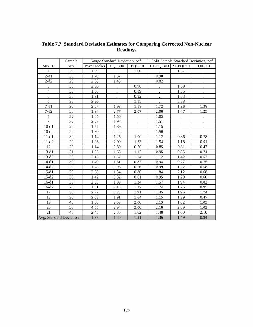
Table 7.7 Standard Deviation Estimates for Comparing Corrected Non-Nuclear Readings
Mix ID Sample
Size Gauge Standard Deviation, pcf Split-Sample Standard Deviation, pcf
PaveTracker PQI 300 PQI 301 PT-PQI300 PT-PQI301 300-301 1 29 1.99 . 1.00 . 1.57 .
2-d1 30 1.70 1.37 . 0.90 . . 2-d2 20 2.08 1.48 . 0.82 . .
3 30 2.06 . 0.98 . 1.59 . 4 30 1.60 . 0.89 . 1.35 . 5 30 1.91 . 0.92 . 1.33 . 6 32 2.80 . 1.15 . 2.28 .
7-d1 30 2.07 1.98 1.18 1.72 1.36 1.38 7-d2 30 1.94 2.77 2.07 2.08 1.47 1.25
8 32 1.85 1.50 . 1.03 . . 9 32 2.27 1.98 . 1.51 . .
10-d1 20 1.57 1.89 . 1.15 . . 10-d2 20 1.80 2.42 . 1.50 . . 11-d1 30 1.14 1.25 1.00 1.12 0.86 0.78 11-d2 20 1.06 2.00 1.33 1.54 1.18 0.91
12 20 1.14 0.89 0.50 0.85 0.81 0.47 13-d1 21 1.33 1.63 1.12 0.95 0.85 0.74 13-d2 20 2.13 1.57 1.14 1.12 1.42 0.57 14-d1 30 1.40 1.31 0.87 0.94 0.77 0.75 14-d2 20 1.28 0.96 0.56 0.99 1.22 0.58 15-d1 20 2.68 1.34 0.86 1.84 2.12 0.68 15-d2 30 1.42 0.82 0.61 0.95 1.20 0.60 16-d1 30 2.53 1.89 1.24 1.57 1.94 0.82 16-d2 20 1.61 2.18 1.27 1.74 1.25 0.95
17 30 2.77 2.23 1.91 1.45 1.96 1.74 18 30 2.08 1.91 1.64 1.15 1.39 0.47 19 46 1.88 2.59 2.00 2.13 1.82 1.03 20 30 4.55 2.94 2.00 2.18 2.89 1.02 21 45 2.45 2.36 1.62 1.48 1.60 2.10
Avg. Standard Deviation 1.97 1.80 1.21 1.36 1.49 0.94
120
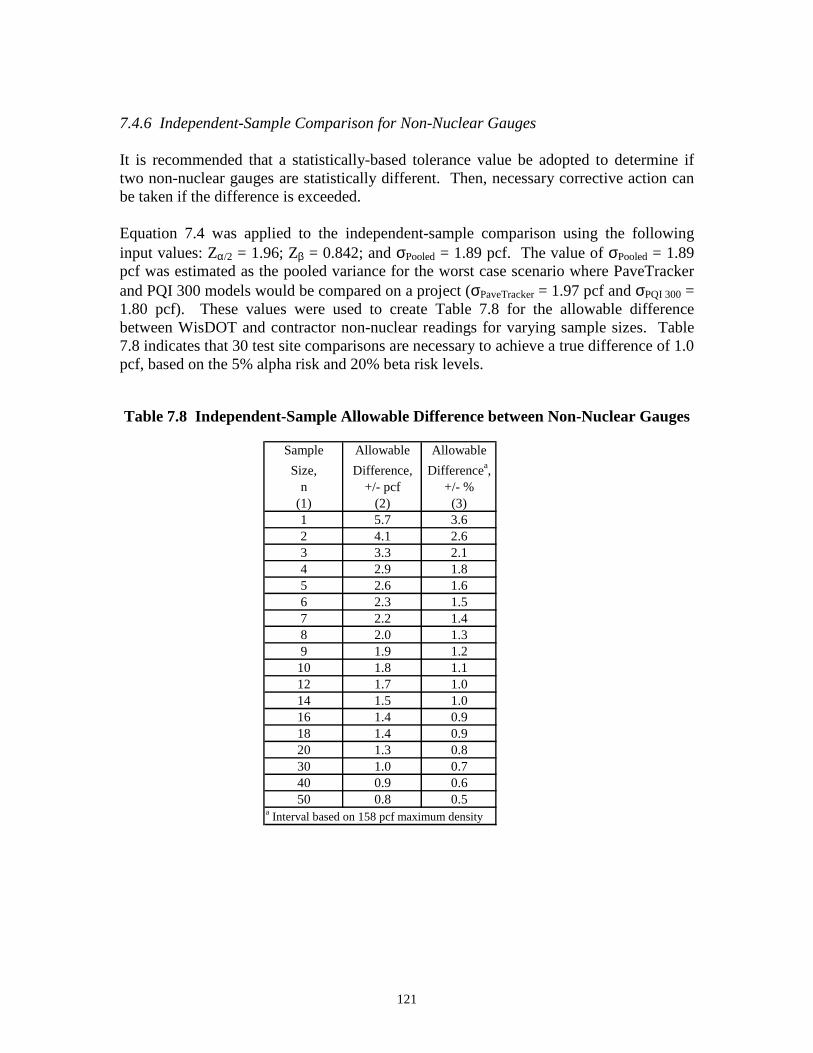
7.4.6 Independent-Sample Comparison for Non-Nuclear Gauges
It is recommended that a statistically-based tolerance value be adopted to determine if two non-nuclear gauges are statistically different. Then, necessary corrective action can be taken if the difference is exceeded.
Equation 7.4 was applied to the independent-sample comparison using the following input values: Zα/2 = 1.96; Zβ = 0.842; and σPooled = 1.89 pcf. The value of σPooled = 1.89 pcf was estimated as the pooled variance for the worst case scenario where PaveTracker and PQI 300 models would be compared on a project (σPaveTracker = 1.97 pcf and σPQI 300 = 1.80 pcf). These values were used to create Table 7.8 for the allowable difference between WisDOT and contractor non-nuclear readings for varying sample sizes. Table 7.8 indicates that 30 test site comparisons are necessary to achieve a true difference of 1.0 pcf, based on the 5% alpha risk and 20% beta risk levels.
Table 7.8 Independent-Sample Allowable Difference between Non-Nuclear Gauges
Sample
Size, n
(1)
Allowable
Difference, +/- pcf
(2)
Allowable
Differencea , +/- %
(3) 1 5.7 3.6 2 4.1 2.6 3 3.3 2.1 4 2.9 1.8 5 2.6 1.6 6 2.3 1.5 7 2.2 1.4 8 2.0 1.3 9 1.9 1.2
10 1.8 1.1 12 1.7 1.0 14 1.5 1.0 16 1.4 0.9 18 1.4 0.9 20 1.3 0.8 30 1.0 0.7 40 0.9 0.6 50 0.8 0.5
a Interval based on 158 pcf maximum density
121
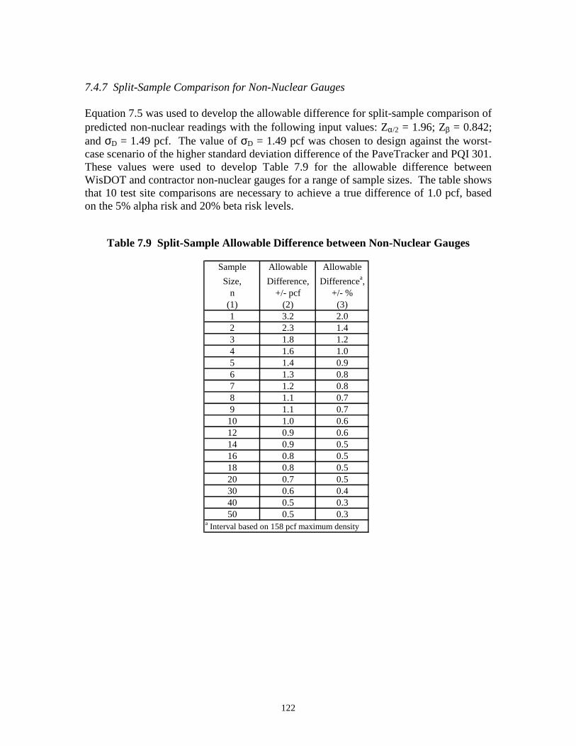
7.4.7 Split-Sample Comparison for Non-Nuclear Gauges
Equation 7.5 was used to develop the allowable difference for split-sample comparison of predicted non-nuclear readings with the following input values: Zα/2 = 1.96; Zβ = 0.842; and σD = 1.49 pcf. The value of σD = 1.49 pcf was chosen to design against the worst-case scenario of the higher standard deviation difference of the PaveTracker and PQI 301. These values were used to develop Table 7.9 for the allowable difference between WisDOT and contractor non-nuclear gauges for a range of sample sizes. The table shows that 10 test site comparisons are necessary to achieve a true difference of 1.0 pcf, based on the 5% alpha risk and 20% beta risk levels.
Table 7.9 Split-Sample Allowable Difference between Non-Nuclear Gauges
Sample
Size, n
(1)
Allowable
Difference, +/- pcf
(2)
Allowable
Differencea , +/- %
(3) 1 3.2 2.0 2 2.3 1.4 3 1.8 1.2 4 1.6 1.0 5 1.4 0.9 6 1.3 0.8 7 1.2 0.8 8 1.1 0.7 9 1.1 0.7
10 1.0 0.6 12 0.9 0.6 14 0.9 0.5 16 0.8 0.5 18 0.8 0.5 20 0.7 0.5 30 0.6 0.4 40 0.5 0.3 50 0.5 0.3
a Interval based on 158 pcf maximum density
122
CHAPTER 8 IMPLEMENTATION
8.1 Introduction
The previous chapter provided recommendations for the new non-nuclear test specification. This chapter presents issues to consider when implementing the new specification.
8.2 Implementation Issues
The primary issues for implementing the non-nuclear test specification are the nuclear density gauge requirement, operator familiarity with the devices, battery charging, adhering to manufacturer recommendations, computing the slope function, test site layout, and training. A brief discussion of each follows.
8.2.1 Nuclear Density Gauges
Nuclear density gauges are a necessary component of the new specification, since they provide the most accurate calibration of the non-nuclear gauges to true pavement density. It was the goal of the study to move away from nuclear gauges; however, nuclear gauges are the only feasible benchmark at this time, aside from cores.
8.2.2 Operator Familiarity
Non-nuclear density gauges are a new technology to Wisconsin paving, and not complicated to operate. Operators should gain rapid familiarity with the gauges, similar to the first experience operating the nuclear density gauge. Immediate benefits of the non-nuclear gauge are lighter weight for the operator, shorter test time, and no nuclear licensing requirement. However, the licensing requirement will be necessary to develop the slope function with the nuclear density gauge.
8.2.3 Battery Life
A charged battery in the non-nuclear gauges lasts approximately 4 to 6 hours, much less than a nuclear gauge battery. The operator will want to recharge the battery after each day of paving, a practice that is not common with nuclear gauges. In addition, the battery compartment is not readily accessible in the non-nuclear gauges; manufacturers should be consulted to change batteries.
123
8.2.4 Manufacturer Recommendations
An important finding in this study was the sensitivity of the non-nuclear readings to moisture index values of about 10. The new test specification must enforce this value, otherwise erroneous readings will be measured. The PQI models have a moisture reading, however, the PaveTracker model lacks this feature. In addition, the 5-point cluster testing within a test site poses a new test method to operators, but can be easily standardized with repeated testing.
8.2.5 Computing the Slope Function
The computations of the daily slope function in the new test procedure are straight forward, and should pose minimal challenges to the technicians operating the non-nuclear gauges. The operator simply divides the 10-point nuclear gauge readings by the 10-point non-nuclear gauge readings. Then, the factor is multiplied by all raw non-nuclear readings. The computations should reside with the field operators, and upper management involvement is not necessary. Slope adjustment computations can be an added component of the WisDOT Highway Technician Certification Program (HTCP) courses.
8.2.6 Test Site Layout
The implementation of a new specification will require a greater effort to layout n=30 test sites, as compared to the current n=7 test sites. Nuclear Density I technicians are familiar with random station and centerline offset computations, so it is a matter of performing more site layout, and not a new method of layout. Computations for the test sites can be updated using current HTCP manuals and practices.
8.2.7 Training
Education and training are key to implementing the new test specification. This report offered detailed explanations of computations, and provided numerous tables with calculations. WisDOT may want to supplement the provided information with additional examples as necessary. Operator training is necessary and should be formalized within the HTCP, most likely in the Nuclear Density I course.
8.2.8 Pilot Program
It is recommended that the new specification be piloted on several projects as soon as possible, to expose the industry to the technology and collect additional data as necessary. It will be necessary to compute a daily slope-adjustment function until data support a move towards a single calibration for a mix design.
124
CHAPTER 9 CONCLUSIONS AND RECOMMENDATIONS
9.1 Conclusions
This report conducted a field evaluation of portable non-nuclear density gauges to determine their effectiveness and practicality for quality control and acceptance of asphalt pavement construction. The following conclusions were reached:
• The literature review of previous field studies generally found a comparison of cores with the non-nuclear Pavement Quality Indicator (PQI) gauge, non-nuclear PaveTracker gauge, and/or a nuclear density gauge. The studies found a bias between cores and both the nuclear and non-nuclear gauges on all projects. Bias, or the difference between the non-nuclear gauge and either the core or nuclear gauge, was generally below 10 pcf. When recommendations were stated in a study, non-nuclear devices could be used for quality control, however, they were not recommended for quality assurance or acceptance testing. Bias correction factors were also recommended using a single additive value.
• Three portable non-nuclear gauge models were evaluated in this study, including the TransTech PQI Models 300 and 301, and Troxler PaveTracker Model 2701b. A CPN MC-3 nuclear density gauge was compared to the non-nuclear gauges; six-inch diameter cores were tested to ensure nuclear gauge calibration. A consistent finding was a bias between nuclear and non-nuclear gauges, and a change in bias within a project between days or a different mix type. All nonnuclear models consistently read lower than the nuclear gauge. PQI Model 301 read 11.2 to 27.2 pcf lower than the nuclear gauge, while PQI Model 300 ranged from 4.2 to 26.6 pcf lower. PaveTracker varied from 1.8 to 17.7 pcf lower.
• An analysis of variance determined that several factors affected the difference between the nuclear and non-nuclear readings, including aggregate source, design ESALs, passing no. 4 sieve, lab air voids, asphalt content, aggregate specific gravity, and pavement layer thickness. The analysis also confirmed that moisture values for PQI models must be below a value of 10, as stated in manufacturer recommendations, to yield valid test results.
• Several other calibration types were investigated, and determined not suitable at this time, including operating the gauges directly after warm up, calibrating to WisDOT test blocks, calibrating to manufacturer reference block, and calibrating to Superpave gyratory specimens. At this time, nuclear density gauges are the only feasible method to calibrate the non-nuclear gauges.
125
• Three calibration functions were investigated using sets of 3, 5, and 10 random points, including the intercept by adding a constant correction factor, slope by multiplying a constant correction factor, and slope-intercept by multiplying a slope term and adding an intercept term. The intercept function, commonly recommended in other studies, had substantially more error with the PQI 300 and was not recommended.
• The stability of the 10-point slope function computed from Day 1 paving was applied to Day 2 raw non-nuclear readings to assess the impact. The results indicated that a Day 2 slope function used to adjust Day 2 readings was more accurate than a Day 1 slope function used to adjust Day 2 readings. PaveTracker produced less error than both PQI models when the Day 1 slope function was applied to Day 2 raw non-nuclear readings.
• The current nuclear density specification was reviewed and analyzed, and it was determined that the current n=7 sample size, coupled with a 95% probability level (5% risk) and mat standard deviation of 2.0 pcf, yielded a confidence interval of ± 1.5 pcf, and ± 0.9 % density. Based on a sample size of n=7 and mat standard deviation of 2.0 pcf, the probability level of the finding the average density within ± 1.0 pcf was estimated to be 81.4%. The probability level of the finding the average within ± 0.5 % density was 70.4%. This indicated that both WisDOT and contractors are exposing themselves to greater risk than the recommended 5% level.
• Sample size for non-nuclear gauge testing for a given lot on project was determined to be n=30 test sites, based on a 95% confidence level, both mat and slope-function error, and confidence intervals of ± 1.0 pcf and ± 0.6 % density. To reduce the confidence interval to ± 0.5 % density, a total of n=50 samples were necessary.
• A procedure for determining the difference between non-nuclear density gauges was detailed. It was determined that when independent sites are used for nonnuclear testing, 30 test site comparisons are necessary to achieve a true difference of 1.0 pcf, based the pooled variance, alpha risk of 5%, and beta risk of 20%. When the same test sites are used for comparison (split sample), 10 comparison test sites are necessary to achieve a true difference of 1.0 pcf, at the same risk levels. The power concept was illustrated to determine the true mean difference between gauges by compensating for alpha and beta risks.
• The primary issues for implementing the non-nuclear test specification were detailed. Several aspects require consideration, including the nuclear density gauge requirement, operator familiarity with the devices, battery charging, adhering to manufacturer recommendations, computing the slope function, test site layout, and training.
126
9.2 Recommendations
The following recommendations were made from the data and analysis presented in this report:
• Adjust the current nuclear density specification if risk levels are to be reduced from current levels of about 20% for the pcf average, and 30% for the percent density average. The sample size should be increased and/or the penalty tolerance be increased.
• Conduct a project-specific calibration between the nuclear and non-nuclear gauges since many of the factors affecting non-nuclear density readings were mixture or project specific. Calibration to only the nuclear density gauge is recommended
• Apply a 10-point calibration using the slope function, rather than the intercept and slope-intercept functions, since it has less error and a more simplistic approach for field purposes. A daily slope function more accurately adjusts non-nuclear readings than using a previous day’s slope function. It is recommended that a daily slope function be computed until future data support a shift to using a previous day’s slope function.
• Specify a sample size for non-nuclear gauge testing of n=30 test sites per lot, based on a 95% confidence level, measured mat variability, slope-function error, and confidence intervals of ± 1.0 pcf and ± 0.6 % density. To reduce the confidence interval to ± 0.5 % density, a total of n=50 samples is recommended.
• Adopt a statistically-based tolerance value, or specified mean difference, that would determine if two non-nuclear devices are statistically different, in order to identify corrective action. Based on the data collected, it is recommended 30 test sites be used for independent sample comparisons, and 10 test sites for split-sample comparisons.
127
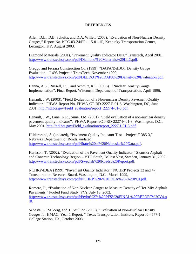
REFERENCES
Allen, D.L., D.B. Schultz, and D.A. Willett (2003), “Evaluation of Non-Nuclear Density Gauges,” Report No. KTC-03-24/FR-115-01-1F, Kentucky Transportation Center, Lexington, KY, August 2003.
Diamond Materials (2001), “Pavement Quality Indicator Data,” Transtech, April 2001. http://www.transtechsys.com/pdf/Diamond%20Materials%20LLC.pdf.
Greggo and Ferrara Construction Co. (1999), “DAPA/DelDOT Density Gauge Evaluation – I-495 Project,” TransTech, November 1999, http://www.transtechsys.com/pdf/DELDOT%20DAPA%20Density%20Evaluation.pdf.
Hanna, A.S., Russell, J.S., and Schmitt, R.L. (1996). “Nuclear Density Gauge Implementation”, Final Report, Wisconsin Department of Transportation, April 1996.
Henault, J.W. (2003), “Field Evaluation of a Non-nuclear Density Pavement Quality Indicator,” FHWA Report No. FHWA-CT-RD-2227-F-01-3, Washington, DC, June 2001, http://ntl.bts.gov/Field_evaluation/report_2227-f-01-3.pdf.
Henault, J.W., Lane, K.R., Sime, J.M. (2001), “Field evaluation of a non-nuclear density pavement quality indicator”, FHWA Report #CT-RD-2227-F-01-3; Washington, D.C., May 2001, http://ntl.bts.gov/Field_evaluation/report_2227-f-01-3.pdf.
Hilderbrand, S. (undated), “Pavement Quality Indicator Test – Project F-385-3,” Nebraska Department of Roads, undated, http://www.transtechsys.com/pdf/State%20of%20Nebraska%20Data.pdf.
Karlsson, T. (2002), “Evaluation of the Pavement Quality Indicator,” Skanska Asphalt and Concrete Technology Region – VTO South, Ballast Vast, Sweden, January 31, 2002. http://www.transtechsys.com/pdf/Swedish%20Roads%20Report.pdf.
NCHRP-IDEA (1999), “Pavement Quality Indicator,” NCHRP Projects 32 and 47, Transportation Research Board, Washington, D.C., March 1999, http://www.transtechsys.com/pdf/NCHRP%20-%20IDEA%20-%20PQI.pdf.
Romero, P., “Evaluation of Non-Nuclear Gauges to Measure Density of Hot-Mix Asphalt Pavements,” Pooled Fund Study, ????, July 18, 2002, http://www.transtechsys.com/pdf/Pedro%27s%20PFS%20FINAL%20REPORT%20V4.p df.
Sebesta, S., M. Zeig, and T. Scullion (2003), “Evaluation of Non-Nuclear Density Gauges for HMAC: Year 1 Report, “ Texas Transportation Institute, Report 0-4577-1, College Station, TX, October 2003.
128
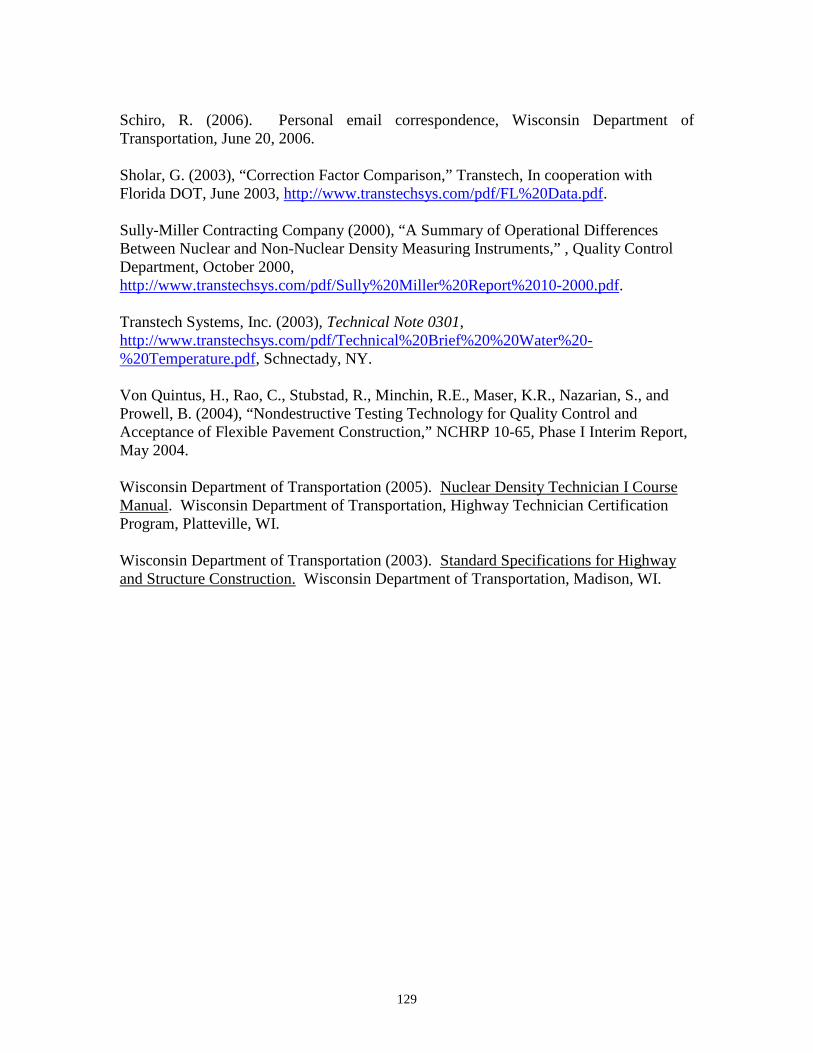
Schiro, R. (2006). Personal email correspondence, Wisconsin Department of Transportation, June 20, 2006.
Sholar, G. (2003), “Correction Factor Comparison,” Transtech, In cooperation with Florida DOT, June 2003, http://www.transtechsys.com/pdf/FL%20Data.pdf.
Sully-Miller Contracting Company (2000), “A Summary of Operational Differences Between Nuclear and Non-Nuclear Density Measuring Instruments,” , Quality Control Department, October 2000, http://www.transtechsys.com/pdf/Sully%20Miller%20Report%2010-2000.pdf.
Transtech Systems, Inc. (2003), Technical Note 0301, http://www.transtechsys.com/pdf/Technical%20Brief%20%20Water%20%20Temperature.pdf, Schnectady, NY.
Von Quintus, H., Rao, C., Stubstad, R., Minchin, R.E., Maser, K.R., Nazarian, S., and Prowell, B. (2004), “Nondestructive Testing Technology for Quality Control and Acceptance of Flexible Pavement Construction,” NCHRP 10-65, Phase I Interim Report, May 2004.
Wisconsin Department of Transportation (2005). Nuclear Density Technician I Course Manual. Wisconsin Department of Transportation, Highway Technician Certification Program, Platteville, WI.
Wisconsin Department of Transportation (2003). Standard Specifications for Highway and Structure Construction. Wisconsin Department of Transportation, Madison, WI.
129
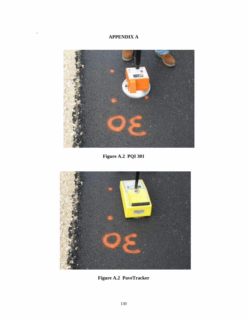
. APPENDIX A
Figure A.2 PQI 301
Figure A.2 PaveTracker
130
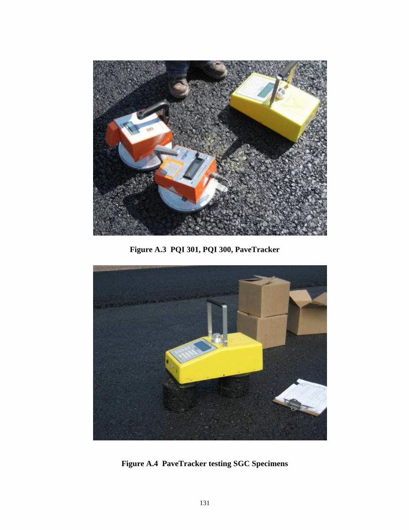
Figure A.3 PQI 301, PQI 300, PaveTracker
Figure A.4 PaveTracker testing SGC Specimens
131