Embed Size (px)
Citation preview
Non-localization of eigenfunctions for Sturm-Liouville
operators and applications
Thibault Liard∗ Pierre Lissy† Yannick Privat‡§
Abstract
In this article, we investigate a non-localization property of the eigenfunctions of Sturm-Liouville operators Aa = −∂xx + a(·) Id with Dirichlet boundary conditions, where a(·) runsover the bounded nonnegative potential functions on the interval (0, L) with L > 0. Moreprecisely, we address the extremal spectral problem of minimizing the L2-norm of a functione(·) on a measurable subset ω of (0, L), where e(·) runs over all eigenfunctions of Aa, at thesame time with respect to all subsets ω having a prescribed measure and all L∞ potentialfunctions a(·) having a prescribed essentially upper bound. We provide some existence andqualitative properties of the minimizers, as well as precise lower and upper estimates on theoptimal value. Several consequences in control and stabilization theory are then highlighted.
Keywords: Sturm-Liouville operators, eigenfunctions, extremal problems, calculus of variations,control theory, wave equation.
AMS classification: 34B24, 49K15, 47A75, 49J20, 93B07, 93B05
1 Introduction
1.1 Localization/Non-localization of Sturm-Liouville eigenfunctions
In a recent survey article concerning the Laplace operator ([10]), D. Grebenkov and B.T. Nguyenintroduce, recall and gather many possible definitions of the notion of localization of eigenfunctions.In particular, in section 7.7 of their article, they consider the Dirichlet-Laplace operator ∆ on agiven bounded open set Ω of IRn, a Hilbert basis of eigenfunctions (ej)j∈IN∗ in L2(Ω) and use as ameasure of localization of the eigenfunctions on a measurable subset ω ⊂ Ω the following criterion
Cp(ω) = infj∈IN∗
‖ej‖pLp(ω)
‖ej‖pLp(Ω)
,
where p > 1. For instance, evaluating this quantity for different choices of subdomains ω if Ω is aball or an ellipse allows to illustrate the so-called whispering galleries or bouncing ball phenomena.At the opposite, when Ω denotes the d-dimensional box (0, `1)× · · · × (0, `d) (with `1, . . . , `d > 0),
∗Universite Pierre et Marie Curie (Univ. Paris 6), CNRS UMR 7598, Laboratoire Jacques-Louis Lions, F-75005,Paris, France ([email protected]).†Ceremade, Universite Paris-Dauphine, CNRS UMR 7534, Place du Marechal de Lattre de Tassigny, 75775 Paris
Cedex 16, France ([email protected]).‡CNRS, Universite Pierre et Marie Curie (Univ. Paris 6), UMR 7598, Laboratoire Jacques-Louis Lions, F-75005,
Paris, France ([email protected]).§The third author is supported by the ANR projects AVENTURES - ANR-12-BLAN-BS01-0001-01 and OPTI-
FORM - ANR-12-BS01-0007
1

it is recalled that Cp(ω) > 0 for any p > 1 and any measurable subset ω ⊂ Ω whenever the ratios(`i/`j)
2 are not rational numbers for every i 6= j.Many other notions of localization have been introduced in the literature. Regarding the
Dirichlet/Neumann/Robin Laplacian eigenfunctions on a bounded open domain Ω of IRn and usinga semi-classical analysis point of view, the notions of quantum limit or entropy have been widelyinvestigated (see e.g. [1, 3, 4, 9, 13, 20]) and provide an account for possible strong concentrationsof eigenfunctions. Notice that the properties of Cp(ω) are intimately related to the behaviorof high-frequency eigenfunctions and especially to the set of quantum limits of the sequence ofeigenfunctions considered. Identifying such limits is a great challenge in quantum physics ([4, 9, 40])and constitute a key ingredient to highlight non-localization/localization properties of the sequenceof eigenfunctions considered.
Given a nonzero integer p, the non-localization property of a sequence (ej)j∈IN∗ of eigenfunctionsmeans that the real number Cp(ω) is positive for every measurable subset ω ⊂ Ω. Concerning theone-dimensional Dirichlet-Laplace operator on Ω = (0, π), it has been highlighted in the case wherep = 2 (for instance in [12, 24, 36]) that
inf|ω|=rπ
C2(ω) = inf|ω|=rπ
infj∈IN∗
2
π
∫
ω
sin(jx)2 dx > 0,
for every r ∈ (0, 1).Motivated by these considerations, the present work is devoted to studying similar issues in
the case p = 2, for a general family of one-dimensional Sturm-Liouville operators of the kind Aa =−∂xx +a(·) Id with Dirichlet boundary conditions, where a(·) is a nonnegative essentially boundedpotential defined on the interval (0, L). More precisely, we aim at providing lower quantitativeestimates of the quantity C2(ω), where (ea,j)j∈IN∗ denotes now a sequence of eigenfunctions of Aa,in terms of the measure of ω and the essential supremum of a(·) by minimizing this criterion atthe same time with respect to ω and a(·), over the class of subsets ω having a prescribed measureand over a well-chosen class of potentials a(·), relevant from the point of view of applications.Independently of its intrinsic interest, the choice “p = 2” is justified by the fact that the quantityC2(ω) plays a crucial role in many mathematical fields, notably the control or stabilization of thelinear wave equation (see for example [25] and [12]) and the randomised observation of linear wave,Schrodinger or heat equations (see for example [33], [37] or [38]).
Explicit lower bounds of C2(ω) have already been obtained in [31] in the case a(·) = 0. In thecase where the potential a(·) differs from 0, some partial estimates of C2(ω) are gathered in [12]holding in a restricted class of potentials with very small variations around constants. Up to ourknowledge, there are no other articles investigating this precise problem.
The article is organized as follows: in Section 1.2, the extremal problem we will investigateis introduced. The main results of this article are stated in Section 2: a comprehensive analysisof the extremal problem is performed, reducing in some sense (that will be made precise in thesequel) this infinite-dimensional problem to a finite one. Moreover, we provide very simple lowerand upper estimates of the optimal value. The whole section 3 is devoted to the proofs of the mainand intermediate results. Finally, consequences and applications of our main results for observationand control theory and several numerical illustrations and investigations are gathered in Section 4.
1.2 The extremal problem
Let L be a positive real number and a(·) be an essentially nonnegative function belonging toL∞(0, L). We consider the operator
Aa := −∂xx + a(·), (1)
2
defined on D(Aa) = H10 (0, L) ∩H2(0, L). As a self-adjoint operator, Aa admits a Hilbert basis of
L2(0, L) made of eigenfunctions denoted ea,j ∈ D(Aa) and there exists a sequence of increasingpositive real numbers (λa,j)j∈IN∗ such that ea,j solves the eigenvalue problem
−e′′a,j(x) + a(x)ea,j(x) = λ2
a,jea,j(x), x ∈ (0, L),
ea,j(0) = ea,j(L) = 0.(2)
By definition, the normalization condition
∫ L
0
e2a,j(x) dx = 1 (3)
is satisfied and we also impose that e′a,j(0) > 0, so that ea,j is uniquely defined.With regards to the explanations of Section 1.1, we are interested in the non-localization prop-
erty of the sequence of eigenfunctions (ea,j)j∈IN∗ . The quantity of interest, denoted J(a, ω), isdefined by
J(a, ω) = infj∈IN∗
∫ωe2a,j(x) dx
∫ L0e2a,j(x) dx
= infj∈IN∗
∫
ω
e2a,j(x) dx, (4)
where ω denotes a measurable subset of (0, L) of positive measure.The real number J(a, ω) is the equivalent for the Sturm-Liouville operators Aa of the quantity
C2(ω) introduced in Section 1.1 for the one-dimensional Dirichlet-Laplace operator.It is natural to assume the knowledge of a priori informations about the subset ω and the
potential function a(·). Indeed, we will choose them in some classes that are small enough to makethe minimization problems we will deal with non-trivial, but also large enough to provide “explicit”(at least numerically) values of the criterion for a large family of potential.
Hence, in the sequel, we assume that:
• the measure (or at least a lower bound of the measure, which leads to the same solution ofthe optimal design problem we consider) of the subset ω is given;
• the potential function a(·) is nonnegative and essentially bounded.
Such conditions are relevant and commonly used in the context of control or inverse problems.Fix M > 0, r ∈ (0, 1), α and β two real numbers such that α < β. Let us introduce the class
of admissible observation subsets
Ωr(α, β) = Lebesgue measurable subset ω of (α, β) such that |ω| = r(β − α), (5)
as well as the class of admissible potentials
AM (α, β) = a ∈ L∞(α, β) such that 0 6 a(x) 6M a.e. on (α, β) , (6)
Let us now introduce the optimal design problem we will investigate.
Extremal spectral problem. Let M > 0, r ∈ (0, 1) and L > 0 be fixed. We consider
m(L,M, r) = infa∈AM (0,L)
infω∈Ωr(0,L)
J(a, ω), (PL,r,M )
where the functional J is defined by (4), Ωr(0, L) and AM (0, L) are respectively definedby (5) and (6).
3

In the sequel, we will call minimizer of the problem (PL,r,M ) a triple (a∗, ω∗, j0) ∈ AM (0, L)×Ωr(0, L)× IN∗ (whenever it exists) such that
infa∈AM (0,L)
infω∈Ωr(0,L)
J(a, ω) =
∫
ω∗ea∗,j0(x)2 dx.
Remark 1. Noting that for a given real number c, the operator Aa + c Id has the same eigenfunc-tions as Aa, we claim that all the results and conclusions of this article will also hold if we replacethe class of potentials AM (α, β) by the larger class
AM (α, β) :=
ρ ∈ L∞(α, β) such that sup
(α,β)
ρ(·)− inf(α,β)
ρ(·) 6M
.
Indeed, for any ρ ∈ AM (0, L), set a = ρ− inf(0,L) ρ. Then, a ∈ AM (0, L), and every eigenfunctioneρ,j solving the system
−e′′ρ,j(x) + ρ(x)eρ,j(x) = µρ,jeρ,j(x), x ∈ (0, L),
eρ,j(0) = eρ,j(L) = 0,
is also a solution of the system
−e′′ρ,j(x) + a(x)eρ,j(x) = λ2
a,jeρ,j(x), x ∈ (0, L),
eρ,j(0) = eρ,j(L) = 0
with λ2a,j = µρ,j + inf(0,L) ρ, whence the claim.
2 Main results and comments
Let us state the main results of this article. The next theorems are devoted to the analysis ofthe optimal design problems (PL,r,M ).
We also stress on the fact that the following estimates of J(a, ω) are valid for every measurablesubset ω of prescribed measure and that we do not need to add any topological assumption on it.
Theorem 1. Let r ∈ (0, 1) and M ∈ IR∗+.
i Problem (PL,r,M ) has a solution (a∗, ω∗, j0). In particular, there holds
m(L,M, r) = mina∈AM (0,L)
minω∈Ωr(0,L)
∫
ω
ea,j0(x)2 dx,
and the solution a∗ of Problem (PL,r,M ) is bang-bang, (i.e. equal to 0 or M a.e. in (0, L)).
ii Assume that M ∈ (0, π2/L2]. Then, ω∗ is the union of j0 + 1 intervals, and a∗ has at most3j0 − 1 and at least j0 switching points1.
Moreover, one has the estimate
γmin(r, r2)3 6 m(L,M, r) 6 r − sin(πr)
π, (7)
with γ = 7√
38 (3− 2
√2) ' 0.2600 and r2 =
√5
5 +√
1010 ' 0.7634.
1Recall that a switching point of a bang-bang function is a point at which this function is not continuous.
4

In the following result, we highlight the necessity of imposing a pointwise upper bound on thepotentials functions a(·) to get the existence of a minimizer.
Theorem 2. Let r ∈ (0, 1) and j ∈ IN∗. Then, the optimal design problem of finding a minimizerto
infa∈A∞(0,L)
infω∈Ωr(0,L)
J(a, ω), (PL,r,∞)
where A∞(0, L) = ∪M>0AM (0, L), has no solution.
We conclude this section by some remarks and comments.
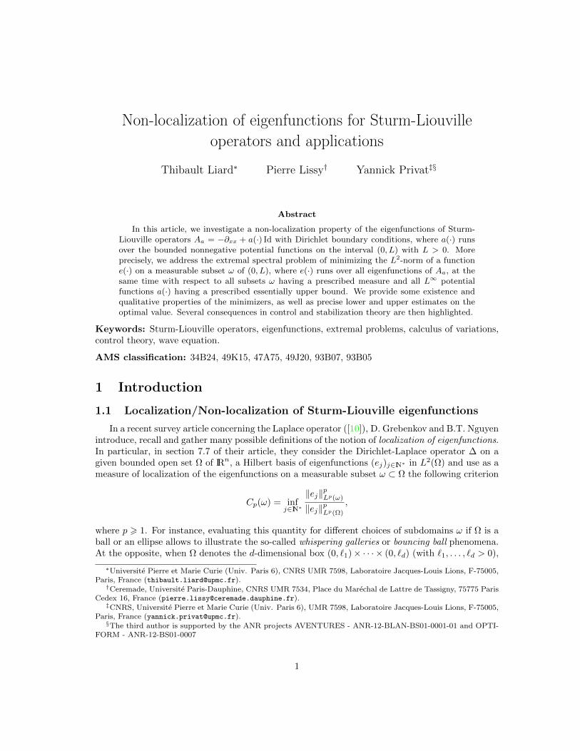
Remark 2. The estimate (7) can be considered as sharp with respect to the parameter r, at leastfor r small enough (which is the most interesting case in view of the applications). Indeed, there
holds πr−sin(πr)π ∼ π2
6 r3 as r tends to 0, which shows that the power of r in the left-hand side
cannot be improved. The graphs of the quantities appearing in the left and right-hand sides of (7)with respect to r are plotted on Figure 1 below.
An interesting issue would thus consist in determining the optimal bounds in the estimate (7),namely
`− = infr∈(0,1)
m(L,M, r)
r3and `+ = sup
r∈(0,1)
m(L,M, r)
r3. (P`−,`+)
It is likely that investigating this issue would rely on a refined study of the optimality conditionsof the problems (P`−,`+), but also of the problem (PL,r,M ). According to (7), we know that
`− ∈ [γ(√
55 +
√10
10 )3, 1] and `+ ∈ [γ, π2/6].
Remark 3. Let us highlight the interest of Theorem 1 for numerical investigations. Indeed, inview of providing numerical lower bounds of the quantity J(a, ω), Theorem 1 enables us to reducethe solving of the infinite-dimensional problems (PL,r,M ) to the solving of finite ones, since onehas just to choose the optimal 3j∗0 − 1 switching points defining the best potential function a∗ andto remark that necessarily ω∗ is uniquely defined once a∗ is defined (since it is defined in terms ofa precise level set of ea∗,j∗0 , see Proposition 1). We will strongly use this remark in Section 4.2.1,where illustrations and applications of Problem (PL,r,M ) are developed.
Remark 4. The restriction on the range of values of the parameter M in the second point ofTheorem 1 makes each eigenfunction ea,j convex or concave on each nodal domain. The upperbound on the parameter M , namely the real number π2/L2 correspond to the lowest eigenvalueof the Dirichlet Laplacian A0. It constitutes a crucial element of the proofs of Theorem 1 andProposition 4, that allows to compare each quantity
∫ωea,j(x)2 dx with the integral of the square
of well-chosen piecewise affine functions. Unfortunately, the solving of Problem (PL,r,M ) whenM > π2/L2 appears much more intricate and cannot be handled with the same kinds of arguments.Some numerical experiments in the case M > π2/L2 will be presented in Section 4.2.
Remark 5. According to Section 4.2.1, numerical simulations seem to indicate that there existsa triple (j∗0 , ω
∗, a∗) solving Problem (PL,r,M )such that j∗0 = 1, the set ω∗ and the graph of a∗ aresymmetric with respect to L/2 and a∗ is a bang-bang function having exactly two switching points.We were unfortunately unable to prove this assertion.
A first step would consist in finding an upper estimate of the optimal index j∗0 . Even this ques-tion appears difficult in particular since it is not obvious to compare the real numbers
∫ωea,j(x)2 dx
for different indices j. One of the reasons of that comes from the fact that the cost functional weconsidered does not write as the minimum of an energy function, making the comparison betweeneigenfunctions of different orders on the subdomain ω intricate.
5

Remark 6. It can be noticed that the lower bound in Proposition 4 is independent of the parameterL. This can be justified by using an easy rescaling argument allowing in particular to restrict ournumerical investigations to the case where L = π (for instance).
Lemma 1. Let j ∈ IN∗, r ∈ (0, 1), M > 0 and L > 0. Then, there holds
infa∈AM (0,π)
infω∈Ωr(0,π)
∫
ω
ea,j(x)2 dx = infa∈AMπ2
L2
(0,L)inf
ω∈Ωr(0,L)
∫
ω
ea,j(x)2 dx, (8)
Remark 7. One can show by using tedious computations inspired by those of Appendix B that thesequences (mj)j∈IN∗ and (rj)j∈IN∗ are increasing. Moreover, straightforward computations showthat (mj)j∈IN∗ converges to 2/3 and (rj)j∈IN∗ converges to 1 as j tends to +∞.
0 0.2 0.4 0.6 0.8 1
0
0.2
0.4
0.6
0.8
1
r
7√3
8(3− 2
√2)min(r,
√5
5+
√10
10)3
r − sin(πr)π
0 5 · 10−2 0.1 0.15 0.2
0
0.5
1
·10−2
r
7√3
8(3− 2
√2)min(r,
√5
5+
√1010
)3
r − sin(πr)π
Figure 1: (Left) Plots of r 7→ γmin(r,√
55 +
√10
10 )3 (thin line) and r 7→ (πr− sin(πr))/π (bold line).(Right) Zoom on the graph for the range of values r ∈ [0, 0.2].
3 Proofs of Theorem 1 and Theorem 2
3.1 Preliminary material: existence results and optimality conditions
We gather in this section several results we will need to prove Theorem 1 and Theorem 2.Let us first investigate the following simpler optimal design problem, where the potential a(·)
is now assumed to be fixed, and which will constitute an important ingredient in the proof.
Auxiliary problem: fixed potential. For a given j ∈ N∗, M > 0, r ∈ (0, 1) anda ∈ AM (0, L), we investigate the optimal design problem
infχ∈Ur
∫ L
0
χ(x)ea,j(x)2 dx, (Aux-Pb)
where the set Ur is defined by
Ur =
χ ∈ L∞(0, L) | 0 6 χ 6 1 a.e. in (0, L) and
∫ L
0
χ(x) dx = rL
. (9)
6
We provide a characterization of the solutions of Problem (Aux-Pb).
Proposition 1. Let r ∈ (0, 1). The optimal design problem Problem (Aux-Pb) has a uniquesolution that writes as the characteristic function of a measurable set ω∗ of Lebesgue measure rL.Moreover, there exists a positive real number τ such that ω∗ is a solution of Problem (Aux-Pb) ifand only if
ω∗ = ea,j(x)2 < τ, (10)
up to a set of zero Lebesgue measure.
In other words, any optimal set, solution of Problem (Aux-Pb), is characterized in terms ofthe level set of the function ea,j(·)2. This result is a direct consequence of [34, Theorem 1] or [39,Chapter 1] and the fact that for every c > 0, the set e2
a,j = c has zero Lebesgue measure, byusing standard properties of eigenfunctions of Sturm-Liouville operators.
The following continuity result is standard. We refer to [32, Chap. 1, page 10] for a proof.
Lemma 2. Let M ∈ IR∗+ and j ∈ N∗. Let us endow the space AM (0, L) with the weak-? topologyof L∞(0, L) 2 and the space H1
0 (0, L) with the standard strong topology inherited from the Sobolevnorm ‖ · ‖H1
0. Then the function a ∈ AM (0, L) 7→ ea,j ∈ H1
0 (0, L) is continuous.
Another key point ouf our proof is the study of the following auxiliary optimal design Problem:
mj(L,M, r) = infa∈AM (0,L)
infω∈Ωr(0,L)
∫
ω
ea,j(x)2 dx, (Pj,L,r,M )
for a fixed j ∈ IN∗.The next result is a direct consequence of Lemma 2.
Proposition 2. Let M ∈ IR∗+, j ∈ IN∗ and r ∈ (0, 1). The optimal design Problem (Pj,L,r,M ) hasat least one solution (a∗j , ω
∗j ).
Proof of Proposition 2. Let us consider a relaxed version of the optimal design Problem(Pj,L,r,M ), where the characteristic function of ω has been replaced by a function χ in Ur (definedin (9)). This relaxed version of (Pj,L,r,M ) writes
inf(a,χ)∈AM (0,L)×Ur
∫ L
0
χ(x)ea,j(x)2 dx.
Let us endow AM (0, L) and Ur with the weak-? topology of L∞(0, L). Thus, both sets are compact.Moreover, according to Lemma 2 and since it is linear in the variable χ, the functional (a, χ) ∈AM (0, L)×Ur 7→
∫ L0χ(x)ea,j(x)2 dx is continuous. The existence of a solution (a∗j , χ
∗j ) follows for
the relaxed problem. Finally, noting that
inf(a,χ)∈AM (0,L)×Ur
∫ L
0
χ(x)ea,j(x)2 dx = infχ∈Ur
∫ L
0
χ(x)ea∗j ,j(x)2 dx,
there exists a measurable set ω∗j of measure rL such that χ∗j = χω∗j , by Proposition 1.
The existence of a solution of Problem (Pj,L,r,M ) is then proved and there holds
inf(a,χ)∈AM (0,L)×Ur
∫ L
0
χ(x)ea,j(x)2 dx = infa∈AM (0,L)
∫
ω∗ea,j(x)2 dx.
2Recall that a sequence (an)n∈IN∗ of L∞(0, L) converges to a for the weak-? topology of L∞(0, L) whenever∫ L0 an(x)ϕ(x) dx converge to
∫ L0 a(x)ϕ(x) dx for every ϕ ∈ L1(0, L).
7
We now state necessary first order optimality conditions that enable us to characterize everycritical point (a∗j , ω
∗j ) of the optimal design problem (Pj,L,r,M ).
Proposition 3. Let j ∈ IN∗, r ∈ (0, 1) and M > 0. Let (a∗j , ω∗j ) be a solution of the optimal design
problem (Pj,L,r,M ) and let
0 = x0j < x1
j < x2j < · · · < xj−1
j < L = xjj (11)
be the j + 1 zeros3 of the j-th eigenfunction ea∗j ,j.
For i ∈ 1 . . . j, let us denote by a∗j,i the restriction of the function a∗j to the interval (xi−1j , xij)
and by ω∗j,i the set ω∗j ∩ (xi−1j , xij). Then, necessarily, there exists τ ∈ IR∗+ such that
• one has ω∗j = ea∗j ,j(x)2 < τ up to a set of zero Lebesgue measure,
• one hasMχpj(x)ea∗
j,j(x)>0(x) 6 a∗j (x) 6Mχpj(x)ea∗
j,j(x)>0(x), (12)
for almost every x ∈ (0, L), where pj is defined piecewisely as follows: for i ∈ 1 . . . j, therestriction of pj to the interval (xi−1
j , xij) is denoted pj,i, and pj,i is the (unique) solution ofthe adjoint system
−p′′j,i(x) + (a∗j,i(x)− λ2a∗j ,j
)pj,i(x) = (χω∗j,i − cj,i)ea∗j ,j , x ∈ (xi−1j , xij),
pj,i(xi−1j ) = pj,i(x
ij) = 0,
(13)
verifying moreover ∫ xij
xi−1j
pj,i(x)ea∗j,i,j(x) dx = 0, (14)
where ˜cj,i is given by
cj,i =
∫ xijxi−1j
χω∗j,i(x)e2a∗j ,j
(x) dx
∫ xijxi−1j
e2a∗j ,j
(x) dx. (15)
In other words, any optimal set solution of Problem (Pj,L,r,M ) is characterized in terms of alevel set of the function ea∗j ,j(·)2 and the optimal potential a∗j is characterized in terms of a level
set of the function pj(·)ea∗j ,j(·).
Remark 8. i According to Fredholm’s alternative (see for example [15]), System (13)-(14)has a unique solution.
ii Another presentation of the first order optimality conditions gathered in Proposition 3 couldhave been obtained by applying the so-called Pontryagin Maximum Principle (see e.g. [27]).
Before proving this proposition, let us state a technical lemma about the differentiability of theeigenfunctions ea,j with respect to a.
3Recall that the family xkj 06k6j is the set of nodal points that are known to be of cardinal j and to be simple
roots of the eigenfunction ea∗,j (see [32, Chap. 2, Thm 6]).
8
Lemma 3. Let us endow the space AM (0, L) with the weak-? topology of L∞(0, L) and the spaceH1
0 (0, L) with the standard strong topology inherited from the Sobolev norm ‖ · ‖H1 . Let a ∈AM (0, L) and Ta,AM (0,L) be the tangent cone4 to the set AM (0, L) at point a. For every h ∈Ta,AM (0,L), the mapping a 7→ ea,j is Gateaux-differentiable in the direction h, and its derivative,denoted ea,j, is the (unique) solution of
−e′′a,j(x) + a(x)ea,j(x) + h(x)ea,j(x) = ˙(
λ2a,j
)ea,j(x) + λ2
a,j ea,j(x), x ∈ (0, L),
ea,j(0) = ea,j(L) = 0,(16)
with ˙(λ2a,j
)=∫ L
0h(x)ea,j(x)2 dx.
The proof of the differentiability is completely standard and is based on the fact that the eigen-values λa,j are simple. For this reason, we skip it and refer to [21, pages 375 and 425].
Proof of Proposition 3. The first point results from Proposition 1.Let us prove the second point.We compute the Gateaux-derivative of the cost functional a 7→
Jω∗j (a), where
Jω∗j (a) = J(a, ω∗j ) =
∫
ω∗j
ea,j(x)2 dx,
at a = a∗j in the direction hj ∈ Ta∗j ,AM (0,L). We denote it by 〈dJω∗j (a∗j ), h〉 and there holds
〈dJω∗j (a∗j ), hj〉 = 2
∫
ω∗ea∗j ,j(x)ea∗j ,j(x) dx,
where ea∗j ,j is the solution of (16).Let us write this quantity in a more convenient form to state the necessary first order optimality
conditions. Let hj be an element of the tangent cone Ta∗j ,AM (0,L). Let us write hj =∑j−1i=1 hj,i
where hj,i = hjχ(xi−1j ,xij)
for all i ∈ 1 . . . j. Hence, hj,i ∈ Ta∗j ,AM (0,L) and there holds
〈dJω∗j (a∗j ), hj〉 =
j∑
i=1
〈dJω∗j (a∗j ), hj,i〉.
It follows that it is enough to consider perturbations with compact support contained in eachnodal domain in order to compute the Gateaux-derivative of Jω∗j . We will use for that purpose the
adjoint state pj piecewisely defined by (13)-(14).Fix i ∈ 1 . . . j and let hj,i be an element of the tangent cone Ta∗j ,AM (xi−1
j ,xij). Let us multiply
the first line of (13) by ea∗j,i,1 and then integrate by parts. We get
∫ xij
xi−1j
e′a∗j,i,1(x)p′j,i(x) + (a∗j,i(x)− λ2a∗j,i,1
)ea∗j,i,1(x)pj,i(x) dx =1
2〈dJ(a∗j ), hj,i〉. (17)
Similarly, let us multiply the first line of (16) by pj,i and then integrate by parts. We get
∫ xij
xi−1j
e′a∗j,i,1(x)p′j,i(x) + (a∗j,i(x)− λ2a∗j,i,1
)eaj,i,1(x)pj,i(x) dx
=˙(
λ2a∗j ,j
)∫ xij
xi−1j
eaj,i,1(x)pj,i(x) dx−∫ xij
xi−1j
hj,i(x)eaj,i,1(x)pj,i(x) dx. (18)
4That is the set of functions h ∈ L∞(0, L) such that, for any sequence of positive real numbers εn decreasing to0, there exists a sequence of functions hn ∈ L∞(0, L) converging to h as n → +∞, and a + εnhn ∈ AM (0, L) forevery n ∈ IN (see for instance [16, chapter 7]).
9
Combining (17) with (18) and using the condition (14) yields
〈dJω∗j (a∗j ), hj,i〉 = −2
∫ xij
xi−1j
hj,i(x)ea∗j,i,1(x)pj,i(x) dx. (19)
As a result, for a general hj ∈ Ta∗j ,AM (0,L), there holds
〈dJω∗j (a∗j ), hj〉 = −2
j∑
i=1
∫ xij
xi−1j
hj,i(x)pj,i(x)ea∗j,i,1 dx = −2
∫ L
0
hj(x)ea∗j ,j(x)pj(x) dx.
Let us state the first order optimality conditions. For every perturbation hj in the cone Ta∗j ,AM (0,L),
there holds 〈dJ(a∗j ), hj〉 > 0, which writes
− 2
∫ L
0
hj(x)ea∗j ,j(x)pj(x) dx > 0. (20)
The analysis of such optimality condition is standard in optimal control theory (see for example[27]) and permits to recover easily (12).
3.2 Proof of Theorem 1
Step 1: existence and bang-bang property of the minimizers (first point of Theorem 1).Notice first that each of the infima defining Problem (PL,r,M ) can be inverted with each other. Asa result, and according to Proposition 2, there exists an optimal pair (a∗j , ω
∗j ) such that
m(L,M, r) = infa∈AM (0,L)
infω∈Ωr(0,L)
J(a, ω) = infj∈IN∗
infa∈AM (0,L)
infω∈Ωr(0,L)
∫
ω
ea,j(x)2 dx
= infj∈IN∗
∫
ω∗j
ea∗j ,j(x)2 dx.
It remains then to prove that the last infimum is reached by some index j0 ∈ IN∗. We will use thetwo following lemmas.
Lemma 4. Let M > 0 and (aj)j∈IN∗ be a sequence of AM (0, L). The sequence (e2aj ,j
)j∈IN∗ converges
weakly-? in L∞(0, L) to the constant function 1L .
The proof of Lemma 4 is standard and is postponed to Appendix A for the sake of clarity. Theproof of the next lemma can be found in [12, 31, 35].
Lemma 5. Let L > 0 and V0 ∈ (0, L). There holds
infρ∈L∞(0,L;[0,1])∫ L
0ρ(x) dx=V0
∫ L
0
ρ(x) sin2
(jπ
Lx
)dx =
1
2
(V0 −
L
πsin(πLV0
)),
for every j ∈ IN∗. Moreover, this problem has a unique solution ρ that writes as the characteristicfunction of a measurable subset ω∗j defined by ω∗j = sin2( jπL ·) 6 ηj for some well-chosen positive
number ηj determined in such a way that the constraint∫ L
0ρ(x) dx = V0 is satisfied.
10
As a consequence of Lemma 5 (which gives the last equality) and by minimality of m(L,M, r)(note that 0 ∈ AM (0, L)), there holds
m(L,M, r) = infj∈IN∗
∫
ω∗j
ea∗j ,j(x)2 dx = infω∈Ωr(0,L)
infj∈IN∗
∫
ω
ea∗j ,j(x)2 dx
6 infω∈Ωr(0,L)
infj∈IN∗
∫
ω
e0,j(x)2 dx =2
Linf
ω∈Ωr(0,L)infj∈IN∗
∫
ω
sin2
(jπ
Lx
)dx
= r − 1
πsin (rπ) .
Using Lemma 4 (the weak-? convergence being used with the “test” function χω∗ ∈ L1(0, L))we have r = limj→+∞
∫ω∗ea∗j ,j(x)2 dx. Thus, m(L,M, r) < limj→+∞
∫ω∗ea∗j ,j(x)2 dx. As a conse-
quence, the infimum infj∈IN∗∫ω∗jea∗j ,j(x)2 dx is reached by a finite integer j∗0 . The existence result
follows.From now on and for the sake of clarity, we will denote by (j0, ω
∗, a∗) instead of (j0, ω∗j0, a∗j0) a
solution of Problem (PL,r,M ). We now prove that the solution a∗ of Problem (PL,r,M ) is bang-bang.Let us write the necessary first order optimality conditions of Problem (PL,r,M ). To simplify thenotations, the adjoint state introduced in Proposition 3 will be denoted by p (resp. pi) instead ofpj0 (resp. pj0,i). For 0 < α < β < L, introduce the sets
• I0,a∗(α, β): any element of the class of subsets of [α, β] in which a∗(x) = 0 a.e.;
• IM,a∗(α, β): any element of the class of subsets of [α, β] in which a∗(x) = M a.e.;
• I?,a∗(α, β): any element of the class of subsets of [α, β] in which 0 < a∗(x) < M a.e., thatwrites also
I?,a∗(α, β) =
+∞⋃
k=1
x ∈ (α, β) :
1
k< a∗(x) < M − 1
k
=:
+∞⋃
k=1
I?,a∗,k(α, β).
We will prove that the set I?,a∗,k(0, L) =⋃ji0=1 I?,a∗,k(xi0−1
j , xi0j ) has zero Lebesgue measure,for every nonzero integer k. Let us argue by contradiction, assuming that one of these setsI?,a∗,k(xi0−1
j , xi0j ) is of positive measure. Let x0 ∈ I?,a∗,k(xi0−1j , xi0j ) and let (Gk,n)n∈IN be a
sequence of measurable subsets with Gn,k included in I?,a∗,k(xi0−1j , xi0j ) and containing x0, the
perturbations a∗ + th and a∗ − th are admissible for t small enough. Choosing h = χGk,n andletting t go to 0, it follows that
〈dJ(a∗), h〉 =
∫ xi0j
xi0−1j
h(x)(−ea∗j ,j(x)pi0(x)
)dx = 0⇐⇒
∫
Gk,n
(−ea∗j ,j(x)pi0(x)
)dx = 0.
Dividing the last equality by |Gk,n| and letting Gk,n shrink to x0 as n → +∞ shows thatea∗j ,j(x0)pi0(x0) = 0 for almost every x0 ∈ I?,a∗,k(xi0−1
j , xi0j ), according to the Lebesgue density
Theorem. Since ea∗j ,j does not vanish on (xi0−1j , xi0j ) we then infer that pi0(x) = 0 for almost
every x ∈ I?,a∗,k(xi0−1j , xi0j ). Let us prove that such a situation cannot occur. The variational
formulation of System (13)-(14) writes: find pi0 ∈ H10 (xi0−1
j , xi0j ) such that for every test function
ϕ ∈ H10 (xi0−1
j , xi0j ), there holds
−∫ x
i0j
xi0−1j
pi0(x)ϕ′′(x) + (ai0(x)− λ2ai0 ,1
)pi0(x)ϕ(x) dx =
∫ xi0j
xi0−1j
(χω∗j,i0− cj,i0)ea∗j ,jϕ(x) dx.
11
Since I?,a∗,k(xi0−1j , xi0j ) is assumed to be of positive measure, let us choose test functions ϕ whose
support is contained in I?,a∗,k(xi0−1j , xi0j ). There holds
∫ L
0
(χω∗j,i0− cj,i0)ea∗j ,j(x)ϕ(x) dx = 0,
for such a choice of test functions, whence the contradiction by using that cj,i0 ∈ (0, 1). We theninfer that |I?,a∗,k(xi0−1
j , xi0j )| = 0 and necessarily, a∗ is bang-bang.
Step 2: counting the switching points of a∗ and the number of connected componentsof ω∗ (first part of the second point of Theorem 1). For the sake of simplicity, we firstgive the argument in the case where the infimum m(L,M, r) is reached at j0 = 1 and we will thengeneralize our analysis to any j0 ∈ IN∗.
At this step, we know that a∗1 is bang-bang and ω∗1 is characterized in terms of the level set ofthe function ea∗1 ,1(·)2. According to (12), the number of switching points of a∗1 corresponds to thenumber of zeros of the function x 7→ p1(x)ea∗1 ,1(x). Let us evaluate this number.
Since M 6 π2/L2, there holds ‖a∗1‖∞ 6 π2
L2 . As a consequence and using (2), one deduces thatthe eigenfunction ea∗! ,1 is concave and reaches its maximum at a unique point xmax ∈ (0, L). More-over, since ea∗1 ,1 is increasing on (0, xmax) and decreasing on (xmax, L) with ea∗1 ,1(0) = ea∗1 ,1(π) = 0,from Proposition 1, there exists (α, β) ∈ (0, L)2 such that α < β and
χω∗1 = 1− χ(α,β), (21)
with α < xmax < β.Let us provide a precise description of the function p1. One readily checks by differentiating
two times the function p1/ea∗1 ,1 that the function p1 may be written as
p1(x) = f(x)ea∗1 ,1(x) (22)
for every x ∈ (0, L), where the function f is defined by
f(x) = −∫ x
0
g(t)dt+ f(0), with f(0) =
∫ L
0
(∫ x
0
g(t)dt
)e2a∗1 ,1
(x) dx (23)
and the function g is defined by
g(t) =
∫ t0(χω∗1 (s)− c)e2
a∗1 ,1(s) ds
e2a∗1 ,1
(t), (24)
where here and in the rest of the proof, we will call c the number c1,1 (whose definition was givenin (15)). In the following result, we provide a description of the function g.
Lemma 6. The function g defined by (24) verifies
g(0) = g(L) = 0, (25)
there exists a unique real number og in (0, L) such that g(og) = 0, (26)
g > 0 in (0, og) and g < 0 in (og, L), (27)
g is decreasing on (α,min(og, xmax)) and (max(og, xmax), β). (28)
12
Proof of Lemma 6. Let us first prove (26). We consider the function g defined by
g(t) =
∫ t
0
(χω∗1 (s)− c)e2a∗1 ,1
(s) ds, (29)
so that the function g writes
g =g
ea∗1 ,1(·)2. (30)
According to (21) and remarking that 0 < c < 1 according to (15), the function g is strictlyincreasing on (0, α) and (β, L), and strictly decreasing on (α, β). Besides, using (15), there holds
g(0) = g(L) = 0. (31)
Hence, using the variations of g given before and (31) that g (and hence g) has a unique zero on(0, L) that we call og from now on. Moreover, clearly g > 0 on (0, og) and g < 0 on (og, L), hence,using (30), we deduce the same property for g and (27) is proved.
Equality (25) is readily obtained by making a Taylor expansion of e2a∗1 ,1
and g around 0 and L
and using (30). Indeed, there holds
e2a∗1 ,1
(x) ∼ x2(e2a∗1 ,1
)′(0) and g(x) ∼ (χω∗1 (0)− c)x3(e2
a∗1 ,1)′(0)/3 as x→ 0,
e2a∗1 ,1
(x) ∼ (x− π)2
2(e2a∗1 ,1
)′(π) and g(x) ∼ (χω∗1 (π)− c)(x− π)3(e2
a∗1 ,1)′(π)/3 as x→ π.
To conclude, it remains to prove (28). From (24), one observes that g is differentiable almosteverywhere on (0, L) and
g′(x) = χω∗1 (x)− c−2e′a∗1 ,1(x)g(x)
ea∗1 ,1(x), (32)
for almost every x ∈ (0, L). Using the variations of ea∗1 ,1, (21) and (32), we infer that g′ is negativealmost everywhere on (α,min(og, xmax)) ∪ (max(og, xmax), β), from which we deduce (28).
As a consequence of (27) and (23), f is strictly decreasing on (0, og) and strictly increasing on(og, L) where og is defined in (26). We conclude that f has at most two zeros in (0, L). Moreover,thanks to (14) and (22), f has at least one zero in (0, L). Since ea∗1 ,1(·) does not vanish in (0, L),one infers that a∗1 has at least 1 and at most 2 switching points.
To generalize our argument to any order j > 2, notice that using the notations of Proposition3 and its proof, one has (−1)i0+1ea∗j,i0 ,1
(x) > 0 for all x ∈ (xi0−1j , xi0j ) with i0 ∈ 1 · · · j. Then,
mimicking the argument above in the particular case where j0 = 1, one shows that the function a∗jhas at most two switching points in (xi0−1
j , xi0j ) and at least one. Besides, since the nodal pointsxiji∈1,···j−1 can also be switching points, we conclude that the function a∗j has at most 3j0− 1
and at least j0 switching points in (0, L).
Step 3: proof of the estimate (7) (last part of the second point of Theorem 1). Letus first show the easier inequality, in other word the right one. It suffices to write that m(L,M, r)is bounded from above by infω∈Ωr(0,L) J(0, ω). Inverting the two infima and using Lemma 5 leadsimmediately to the desired estimate.
The left inequality appears more intricate to establish. It is in fact inferred from a more preciseestimate for the optimal design problem (Pj,L,r,M ). Because of its intrinsic interest, we state thisestimate in the following proposition, which constitutes therefore an essential ingredient for theproof of the last point of Theorem 1.
13

Proposition 4. Let r ∈ (0, 1) and let us assume that M ∈ (0, π2/L2]. Then, there holds
mj(L,M, r) > min(r, rj)3mj , (33)
for every j ∈ IN∗, where the sequences (mj)j∈IN∗ and (rj)j∈IN∗ are defined by
mj =
12 if j = 1,
(2j2−1)(j2−1)32
(√j2
j2−2−1
)2
3j3
((j2
j2−2
) j2−1
)2 if j > 2,
and
rj =
1 if j = 1,(j+√j2−2
2√j2+1
)(j − (j2−2)
j2
jj−1
)if j > 2.
The proof of this proposition is quite long and technical but the method is elementary andinteresting. For this reason, we will temporarily admit this result and postpone its proof toSection 3.3. Let us assume for the moment that r 6 r2. Let us notice that m2 = 7
8
√3(3 − 2
√2)
and r2 =√
55 +
√10
10 . Then, it just remains to prove that mj > m2 and rj > r2 for everyj ∈ IN\0, 1.
Proof of mj > m2: We introduce the function F defined on [2,+∞) by
F (x) =
(2x2 − 1)(x2 − 1)3/2
((x2
x2−2
)1/2
− 1
)2
x3
((x2
x2−2
)x/2− 1
)2 .
Notice that F (j) = 3mj for every j ∈ IN∗. Let us write F (x) = u(x)v(x) with
u(x) =
(2x2 − 1)
((x2
x2−2
)1/2
− 1
)2
((x2
x2−2
)x/2− 1
)2 and v(x) =(x2 − 1)3/2
x3.
Let us show that u(x) > u(2) for every x > 2. This comes to show that ψ(x) 6 0, where
ψ(x) = γ
((x2
x2 − 2
)x/2− 1
)−√
2x2 − 1
((x2
x2 − 2
)1/2
− 1
),
with γ =√u(2) =
√7(√
2− 1), for every x > 2. The derivative of ψ writes
ψ′(x) = γ
(x2
x2 − 2
)x/2w(x)− 2x√
2x2 − 1
(√x2
x2 − 2− 1
)−√
2x2 − 1
(x2 − 2)3/2,
with w(x) = ln(√
x2
x2−2
)− 1
x2−2 . The derivative of w writes w′(x) = 4x(x2−2)2 , and therefore,
the function w is increasing and negative since limx→+∞ w(x) = 0. One then infers that ψ′(x)writes as the sum of three negative terms and is thus negative on [2,+∞). Hence, the function
14
ψ decreases on this interval and therefore, ψ(x) 6 ψ(2) = 0 for every x ∈ [2,+∞). The expectedresult on u follows.
Let us now show that v(x) > v(2) for every x ∈ [2,+∞). The derivative of v writes
v′(x) =3√x2 − 1
x4,
is therefore positive on [2,+∞), and the expected conclusion follows.
Proof of rj > r2: Let us write rj = u(j)v(j) with
u(j) =j +
√j2 − 2
2√j2 + 1
and v(j) = j − (j2 − 2)j2
jj−1.
We claim that j 7→ u(j) is a increasing function for every j > 2 and j 7→ v(j) is a increasingfunction for every j > 4. Indeed, straightforward computations show that
∀j > 2,du
dj(j) =
(j +√j2 − 2)(j2 + 1− j
√j2 − 2)
2√j2 − 2(j2 + 1)3/2)
> 0
and
∀j > 4,dv
dj(j) =
(jj−1 + (j2 − 2)j/2(ln(√
γ(j))− γ(j) + 1− 1
j )
jj−1> 0
We thus infer that for every j > 4, there holds g(j − 1, j) > g(3, 4). Dealing separately with thecases j = 2 and j = 3 leads to the desired conclusion for r 6 r2.
Let us now treat the case r > r2. It is obvious that the solution (a, ω) of the following problem
infa∈AM (0,L)
infω∈Ωr(0,L)
J(a, ω), (PL,r,M )
where
Ωr(α, β) = Lebesgue measurable subset ω of (α, β) such that |ω| > r(β − α),satisfies in particular that ω ∈ Ωr(0, L) (in other words, the inequality constraint is reached at theoptimum). Therefore, the problems (PL,r,M ) and (PL,r,M ) are the same.
Taking into account this new expression, we remark that the quantity m(L,M, r) is nonde-creasing with respect to r and so for r > r2 we have m(L,M, r) > m(L,M, r2) > m2r
32, which
concludes the proof.
3.3 Proof of Proposition 4
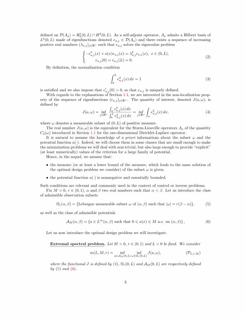
The proof, although quite technical, is based on a simple idea: by using the concavity of theeigenfunction ea,j on each nodal domain, we will determine a piecewise affine function ∆j suchthat ea,j > ∆j for every a ∈ AM (0, L). The construction of such a function is not obvious sinceone has to control at the same time the slope of the graph of ∆j on each interval on which it isaffine, and its maximum, as the potential a describes the set AM (0, L).
As previously, we will first consider the case where j = 1. In other words, we will first providea lower estimate of the quantity m1(L, r). We will then generalize this estimate to any j ∈ IN∗ byusing that the j-th eigenfunction ea,j of Aa coincides with the first eigenfunction of the restrictionof Aa on each nodal domain.
Notice that, proving that the estimate (33) holds for every M ∈ (0, π2/L2] is equivalent toshowing it for the particular value
M = π2/L2,
which will be assumed from now on. Let a be a generic element of AM (0, L).
15
First step: proof of Proposition 4 in the case “j = 1”. By using the concavity of ea,1we will construct an affine function ∆1 (see Figure 2) such that ea,1 > ∆1 pointwisely on [0, L].We will infer a lower bound of m1(L,M, r) by computing explicitly the minimum of the quantity∫ω
∆21(x) dx over the class of measurable subsets ω of (0, L) such that |ω| = rL. For that purpose,
let us first provide an estimate of the max(0,L) ea,1 in terms of the L2 norm of ea,1 and the derivativesof ea,1 at x = 0 and x = L.
Lemma 7. With the assumptions of Proposition 4, there holds
e2a,1(xmax) > max
3
2L
∫ L
0
e2a,1(x) dx,
L2
2π2maxe′a,1(0)2, e′a,1(L)2
. (34)
Proof of Lemma 7. Since e′a,1(xmax) = 0, multiplying Equation (2) by e′1 and integrating on(x, xmax) (with possibly x > xmax) leads to
e′a,1(x)2 =
∫ xmax
x
(λ2a,1 − a(x))
d
dx(e2a,1(x)) dx (35)
for every x ∈ (0, L). Besides, according to the Courant-Fischer minimax principle (see for instance[Section C, (90)]) , one has
0 6 λ2a,1 − a(·) 6 2π2
L2in (0, L). (36)
Therefore, combining (35) and (36) yields
e′a,1(x)2 62π2
L2(e2a,1(xmax)− e2
a,1(x)), (37)
for every x ∈ (0, L). In particular, applying (37) at x = L and x = 0, we obtain
maxe′a,1(L)2, e′a,1(0)2 6 2π2
L2e2a,1(xmax), (38)
Moreover, by integrating (37) between 0 and L, we obtain
∫ L
0
e′a,1(x)2 dx+2π2
L2
∫ L
0
e2a,1(x) dx 6
2π2
L2e2a,1(xmax)L. (39)
We obtain (34) from (38) and by combining (39) with Poincare’s inequality
∫ L
0
ea,1(x)2 dx 6L2
π2
∫ L
0
e′a,1(x)2 dx.
According to (34), and assuming since the eigenfunction ea,1 is normalized in L2(0, L), thereholds
e2a,1(xmax) >
3
2L. (40)
Since ea,1 is concave and according to (40), one has the successive inequalities
ea,1(x) > Tra,1(x) > ∆1(x), (41)
16

Lα∗ β∗
(1− r)L
xmax
ea,1(xmax)
√32L
0
41
Tra,1
Figure 2: Graphs of the functions ea,1, Tra,1 and ∆1.
for every x ∈ [0, L], where Tra,1 and ∆1 denote the piecewise affine functions defined by
Tra,1(x) =
ea,1(xmax)x
xmaxon (0, xmax)
ea,1(xmax)(L−x)L−xmax on (xmax, L)
and ∆1(x) =
√3x√
2Lxmaxon (0, xmax)
√3(L−x)√
2L(L−xmax)on (xmax, L).
Combining (40) with (41) and according to Proposition 1, we readily obtain
infω∈Ωr(0,L)
∫
ω
ea,1(x)2 dx > infω∈Ωr(0,L)
∫
ω
∆1(x)2dx =
∫
ω
∆1(x)2dx, (42)
with ω = (0, α∗) ∪ (β∗, L) verifying
∆1(α∗) = ∆1(β∗) and |ω| = L− β∗ + α∗ = rL.
It follows that α∗ = rxmax, β∗ = (1− r)L+ rxmax and one obtains
∫
ω
∆1(x)2 dx =
∫ rxmax
0
∆1(x)2 dx+
∫ L
(1−r)L+rxmax
∆1(x)2 dx =r3
2= r3m1. (43)
We have then proved Proposition 4 in the case where j = 1.
Second step: proof of Proposition 4 in the general case. We now assume that j > 2.Let 0 = x0
j < x1j < x2
j < · · · < xj−1j < L = xjj be the j + 1 zeros of the j-th eigenfunction ea,j .
Introduce γ = (γ1, · · · , γj−1) ∈ (0, 1)j such that
γi =
∫ xi+1j
xij
e2a,j(x) dx, i = 0, . . . , j − 1. (44)
Note that, because of the normalization condition on the function ea,j , there holds
j−1∑
i=0
γi = 1. (45)
In the sequel, we will use the following notations, for all i ∈ 0, · · · , j − 1,
Ωi = (xij , xi+1j ), ηi =
|Ωi|L∈ (0, 1), and ea,j(x
imax) = max
x∈Ωiea,j(x). (46)
17
Now, assume that r 6
(j+√j2−2
2√j2+1
)(j − (j2−2)
j2
jj−1
). We will distinguish between several cases,
depending on the value of the first integer i0 ∈ 0, · · · , j−1 (that exists thanks to (45)) such that
γi0 >1
j. (47)
By exploiting condition (47), we will yield a lower bound Ai0 of the positive number |ea,j(xi0max)|.Then we will derive an estimate of ea,j(x
i0−1max ) and ea,j(x
i0+1max ) in terms of ea,j(x
i0max). Hence, step
by step we will get lower bounds of all j maxima needed to construct the piecewise affine function∆j . For that purpose, we have to distinguish between several cases, depending on the value of theinteger i0
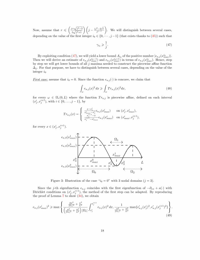
First case: assume that i0 = 0. Since the function ea,j(·) is concave, we claim that
∫
ω
ea,j(x)2 dx >∫
ω
Tra,j(x)2dx, (48)
for every ω ∈ Ωr(0, L) where the function Tra,j is piecewise affine, defined on each interval(xij , x
i+1j ), with i ∈ 0, . . . , j − 1, by
Tra,j(x) =
x−xijximax−xij
ea,j(ximax) on (xij , x
imax),
xi+1j −x
xi+1j −ximax
ea,j(ximax) on (ximax, x
i+1j ),
for every x ∈ (xij , xi+1j ).
ea,3(x1max)
ea,3(x2max)
ea,3(x3max)
x03x13 x23 Lx0max
Ω0
Ω1
x1max
Ω2
Figure 3: Illustration of the case “i0 = 0” with 3 nodal domains (j = 3).
Since the j-th eigenfunction ea,j coincides with the first eigenfunction of −∂xx + a(·) withDirichlet conditions on (xij , x
i+1j ), the method of the first step can be adapted. By reproducing
the proof of Lemma 7 to show (34), we obtain
ea,j(ximax)2 > max
2π2
|Ωi|2 + π2
L2(π2
|Ωi|2 + π2
L2
)|Ωi|
∫ xi+1j
xij
ea,j(x)2 dx,1
π2
|Ωi|2 + π2
L2
maxe′a,j(xij)2, e′a,j(xi+1j )2
.
(49)
18
Notice that one recovers (34) by substituting |Ωi| by L in (49). One derives from the equivalent of(37) in this case the estimates
π2
|Ωi|2− π2
L26
e′a,j(xij)
2
ea,j(ximax)26
π2
|Ωi|2+π2
L2and
π2
|Ωi|2− π2
L26
e′a,j(xi+1j )2
ea,j(ximax)26
π2
|Ωi|2+π2
L2. (50)
Applying (49) for i = 0 and using (47) yields
ea,j(x0max)2 > A0 with A0 =
2π2
|Ω0|2 + π2
L2
j(
π2
|Ω0|2 + π2
L2
)|Ω0|
=1
Lj
(2 + η2
0
η0(1 + η20)
). (51)
Let us now provide an estimate of ea,1(x1max)2. Combining the inequalities (49) with i = 1 and
(50) with i = 0, we get
ea,1(x1max)2 >
e′a,j(x1j )
2
π2
|Ω1|2 + π2
L2
>( π2
|Ω0|2 −π2
L2 )ea,1(x0max)2
π2
|Ω1|2 + π2
L2
. (52)
Combining (51) and (52) yields
ea,j(x1max)2 > A1 with A1 =
(L2 − |Ω0|2)|Ω1|2(L2 + |Ω1|2)|Ω0|2
A0 =(1− η2
0)η21
(1 + η21)η2
0
A0.
By induction, it follows that
ea,j(ximax)2 > Ai with Ai =
(i∏
k=1
(1− η2k−1)η2
k
(1 + η2k)η2
k−1
)A0, (53)
for every i ∈ 1, · · · , j − 1. Hence, (53) together with (48) allows us to write∫
ω
ea,j(x)2 dx >∫
ω
∆j(x)2 dx,
where ∆j is the piecewise affine function defined on (0, L) by
∆j(x) =
(x−xij)(ximax−xij)
√Ai on (xij , x
imax),
(xi+1j −x)
(xi+1j −ximax)
√Ai on (ximax, x
i+1j ),
(54)
for every i ∈ 0, · · · , j − 1 and x ∈ (xij , xi+1j ) (see Fig. 4 below).
According to Proposition 1, we obtain
infω∈Ωr(0,L)
∫
ω
ea,j(x)2 dx > infω∈Ωr(0,L)
∫
ω
∆j(x)2 dx =
∫
ω
∆j(x)2 dx, (55)
where ω = ∆j(x)2 < τ up to a set of zero Lebesgue measure and |ω| = rL. Let i ∈ 0, · · · , j−1and let us introduce ωi = ω ∩ (xij , x
i+1j ).
The following technical Lemma allows to deal with small values of the parameter r.
Lemma 8. Let j > 1, L, τ > 0, let r ∈ (0, 1) such that |ω| = rL, where ω = ∆2j (·) < τ,
with ∆j defined by (54). Recall that A0 is defined by (51) and Ai is defined by (53) for everyi ∈ 1, · · · , j − 1. There holds
r <
(j +
√j2 − 2
2√j2 + 1
)(j − (j2 − 2)
j2
jj−1
)=⇒ τ 6 min
i∈0,··· ,j−1Ai.
19

ea,3(x1max)
ea,3(x2max)
ea,3(x3max)
x03x13 x23
√A0
−√|A1|
√A2
∆j
L
A0
A1
A2
A3
x14 x24 x34
τ
Figure 4: Left: graphs of the functions ea,3 and ∆3. Right: j = 4. Graph of ∆24 with respect to x.
The proof Lemma 8 is postponed to Section B. As a consequence of this lemma, there existα∗i , β
∗i and ri ∈ (0, 1) such that ωi = (xij , α
∗i )∪ (β∗i , x
i+1j ), |ωi| = ri(x
i+1j − xij) (see Figure 4 for an
illustration), and thereforej−1∑
i=0
ri(xi+1j − xij) = rL. (56)
By definition of ω, one has ∆2j (α∗i ) = ∆2
j (β∗i ) = ∆2
j (α∗i+1), consequently there holds
α∗i = ri(ximax − xij) + xij , β∗i = xi+1
j − ri(xi+1j − ximax), (57)
andr2i+1Ai+1 = r2
iAi = · · · = r20A0. (58)
As a result, one obtains
∫
ω∗∆j(x)2 dx =
j−1∑
i=0
∫
ωi
∆j(x)2 dx =1
3
j−1∑
i=0
r3i |Ωi|Ai. (59)
To compute the numbers ri, we use (58) together with (53), which yields to
ri =
√A0
Air0 =
√√√√i∏
k=1
(1 + η2k)η2
k−1
(1− η2k−1)η2
k
r0. (60)
Since∑j−1i=0 ri
|Ωi|L =
∑j−1i=0 riηi = r, one infers
r0 =r
η0 +∑j−1i=1 ηi
√∏ik=1
(1+η2k)η2k−1
(1−η2k−1)η2k
=r
η0
(1 +
∑j−1i=1
√∏ik=1
(1+η2k)
(1−η2k−1)
) . (61)
Besides, using (60), there holds
j−1∑
i=0
r3i |Ωi|Ai = r2
0A0
j−1∑
i=0
ri|Ωi| = r20A0rL. (62)
We conclude by combining (62) with (59) that∫
ω
∆j(x)2 dx =1
3A0r
20rL, (63)
20
where A0 and r0 are respectively given by (51) and (61).Since our goal is to estimate
∫ω
∆j(x)2 dx from below, regarding (63), we need to find a lowerbound on r0 and consequently on the numbers |Ωi| according to (62). We will use the followingLemma.
Lemma 9. For every i ∈ 0, · · · , j − 1, there holds
L√j2 + 1
6 |Ωi| 6L√j2 − 1
. (64)
Proof of Lemma 9. According to the Courant-Fischer minimax principle, one has
jπ
L6 λa,j 6
√(jπ
L
)2
+π2
L2.
Since the j-th eigenfunction ea,j is also the first eigenfunction of the operator −∂xx + a(·) withDirichlet boundary conditions on Ωi, we also have
π
|Ωi|6 λa,j 6
√(π
|Ωi|
)2
+π2
L2.
We then inferπ√(
jπL
)2+ π2
L2
6 |Ωi| 6π√(
jπL
)2 − π2
L2
.
It follows from Lemma 9 that 1√j2+1
6 ηi 6 1√j2−1
and therefore
j−1∑
i=1
√√√√i∏
k=1
(1 + η2k)
(1− η2k−1)
6 g1(j),
where g1(j) =∑j−1i=1
(j2
j2−2
) i2
=
(j2
j2−2
) j2−(
j2
j2−2
) 12(
j2
j2−2
) 12−1
. According to (61), one has
r0 >r
η0(1 + g1(j)). (65)
Combining (51), (63) and (65), we obtain∫
ω
∆j(x)2 dx > r3 infη0∈
(1√j2+1
, 1√j2−1
) g2(η0, j), (66)
with
g2(η0, j) =1
3j
(2 + η2
0
η0(1 + η20)
)(1
η0 + η0g1(j)
)2
.
Since for every η0 > 0, we have
∂g2
∂η0(η0, j) = −
(√j2
j2−1 − 1)2 (
11η20 + 3η4
0 + 6)
(( j2
j2−1 )j2 − 1
)2
η40(1 + η2
0)2j6 0,
21

the function η0 7→ g2(η0, j) is decreasing, so that (66) becomes
∫
ω
∆j(x)2 dx > r3g2
(√1
j2 − 1, j
)= r3mj , (67)
and the expected result is proved for r 6 rj :=
(j+√j2−2
2√j2+1
)(j − (j2−2)
j2
jj−1
).
Noticing that r 7→ infω∈Ωr(0,L)
∫ω
∆j(x)2dx is an increasing function, we infer that for everyr ∈ [rj , 1], there holds
infω∈Ωr(0,L)
∫
ω
∆j(x)2 dx > infω∈Ωrj (0,L)
∫
ω
∆j(x)2dx > r3jmj ,
and the expected result is proved for r ∈ [0, 1].
Second case: assume now that i0 = 1. We will prove that the estimate choosing i0 = 0 is worstthan the estimate that we obtain with i0 = 1. Using (49) with i = 1, we have
e2a,j(x
1max) > A1 with A1 =
1
Lj
(2 + η2
1
η1(1 + η21)
). (68)
Combining the inequality (49) with i = 0, (50) with i = 1 and (68) we get
A0 =(1− η2
1)η20
(1 + η20)η2
1
A1. (69)
Using (49) with i = 2, (50) with i = 1 and (68) we have
e2a,j(x
2max) > A2 with A2 =
(1− η21)η2
2
(1 + η22)η2
1
A1.
By induction, for every i ∈ 2, · · · , j − 1 we have
e2a,j(x
imax) > Ai with Ai =
(i∏
k=2
(1− η2k−1)η2
k
(1 + η2k)η2
k−1
)A1 (70)
Let us state the equivalent of Lemma 8 for the case considered here.
Lemma 10. Let j > 1, L, τ > 0, let r ∈ (0, 1) such that |ω| = rL, where ω = ∆2j (·) < τ, with
∆j is defined by (54). Recall that A1 is defined by (68), A0 is defined by (69) and Ai is defined by(70) for every i ∈ 2, · · · , j − 1. There holds
r <
(j +
√j2 − 2
2√j2 + 1
)(j − (j2 − 2)
j2
jj−1
)=⇒ τ 6 min
i∈0,··· ,j−1Ai.
The proof of this lemma is postponed to Section B.Hence, we conclude that r2
iAi = r21A1 for all i ∈ 0, · · · , j − 1. Since
∑j−1i=0 riηi = r, one
computes by using (70) and (69)
r1 =r
η1 + η0
√A1
A0+∑j−1i=2 ηi
√A1
Ai
=r
η1 + η0
√1+η201−η21
+∑j−1i=2 ηi
√∏ik=2
(1+η2k)η2k−1
(1−η2k−1)η2k
.
22
Moreover, one hasj−1∑
i=2
ηi
√√√√i∏
k=2
(1 + η2k)η2
k−1
(1− η2k−1)η2
k
= η1
j−1∑
i=2
√√√√i∏
k=2
1 + η2k
1− η2k−1
and since 1√j2+1
6 ηi 6 1√j2−1
according to Lemma 9, there holds
r1 >r
η1 + η1
√j2
j2−2 + η1
∑j−1i=2
(j2
j2−2
) i−12
.
Since j > 2, we have
√j2
j2 − 2+
j−1∑
i=2
(j2
j2 − 2
) i−12
−j−1∑
i=1
(j2
j2 − 2
) i2
=
√j2
j2 − 2−(
j2
j2 − 2
) j−12
6 0,
and it follows thatr1 >
r
η1 + η1
∑j−1i=1
(j2
j2−2
) i2
.
As a consequence, using the same approach as the one used for the case where i0 = 0, we inferthat
infω∈Ωr(0,L)
∫
ω
∆j(x)2 dx > r3 infη1∈
(1√j2+1
, 1√j2−1
) g2(η1, j)
with
g2(η1, j) =1
3j
(2 + η2
1
η1(1 + η21)
)(1
η1 + η1g1(j)
)2
and g1(j) =
(j2
j2−2
) j2 −
(j2
j2−2
) 12
(j2
j2−2
) 12 − 1
.
Noticing that the functions g1 and g2 are exactly the same as in the case i0 = 1, we concludesimilarly to the first case.
Finally, mimicking this proof and adapting it for every i0 ∈ 2, · · · , j − 1, we prove that theestimate with i0 = 0 is the worst one. We then obtain the same conclusion.
3.4 Proof of Theorem 2
We argue by contradiction, assuming that the optimal design problem (PL,r,∞) has a solutiona∗ ∈ L∞(0, L). Then, denoting M0 = ‖a∗‖L∞(0,L) and noting that AM0
(0, L) is included inA∞(0, L), it follows that a∗ is a solution of the problem
infa∈A∞(0,L)
infω∈Ωr(0,L)
J(a, ω) = infa∈AM0
(0,L)inf
ω∈Ωr(0,L)
∫
ω
ea,j(x)2 dx,
for some given nonzero integer j, by using the same argument as in the first step of the proof ofTheorem 1 to show the existence of a minimizing integer.
We will use the notations of Proposition 3 and Section 3.2. The contradiction will be obtainedby constructing a perturbation a∗n of a∗ such that J(a∗n) < J(a∗). According to Proposition 3, a∗
23
is non-trivial and bang-bang, equal to 0 and M0 almost everywhere in (0, L) so that there existsi0 ∈ 1, · · · , j such that the set IM0,a∗(x
i0−1j , xi0j ) is measurable of positive measure.
Thanks to the regularity of the Lebesgue measure, there exists an increasing sequence of com-pact sets (Kn)n∈IN strictly included in IM0,a∗(x
i0−1j , xi0j ) satisfying
limn→∞
|Kn| = |IM0,a∗(xi0−1j , xi0j )|,
where | · | denotes the Lebesgue measure. In what follows, we will use the notation Ic to denotethe complement of any set I ⊂ [0, L] in [0, L]. We introduce
a∗n(x) =
M0 + 1
ϕ(n) on Kn,
0 on Kcn,
with ϕ(n) = |IM0,a∗(xi0−1j , xi0j ) ∩Kc
n|.
Let us remark that
a∗n(x)− a(x) =
1ϕ(n) on Kn,
−M0 on IM0,a∗(xi0−1j , xi0j ) ∩Kc
n,
0 on IM0,a∗(xi0−1j , xi0j )c.
Hence, we get
〈dJ(a), ϕ(n)(a∗n − a∗)〉 = −2
∫ xi0j
xi0−1j
ϕ(n)(a∗n(x)− a∗(x))eai0 ,1(x)pi0(x) dx
= 2M0ϕ(n)
∫
IM0,a∗ (x
i0−1j ,x
i0j )∩Kc
n
eai0 ,1(x)pi0(x) dx
−∫
Kn
eai0 ,1(x)pi0(x) dx,
for n ∈ IN. Using (12), we have eai0 ,1pi0 > 0 on IM0,a∗(xi0−1j , xi0j ) ∩Kc
n and eai0 ,1pi0 > 0 on Kn
for all n ∈ IN. Since limn→+∞ ϕ(n) = 0 and according to the Lebesgue density theorem,
limn→+∞
2M0ϕ(n)
∫
IM0,a∗ (x
i0−1j ,x
i0j )∩Kc
n
eai0 ,1(x)pi0(x) dx = 0.
As a consequence, there exists n0 ∈ IN such that for all n > n0 〈dJ(a), ϕ(n)(a∗n − a∗)〉 < 0. Thus,there exists n1 ∈ IN verifying J(a∗n1
) < J(a∗), whence the contradiction. We then infer that theoptimal design problem (PL,r,∞) has no solution.
4 Applications and numerical investigations
4.1 Controllability issues for the wave equation
4.1.1 The cost of the control in large time
Let us fix T > 0 and consider the one dimensional wave equation with potential
∂ttϕ(t, x)− ∂xxϕ(t, x) + a(x)ϕ(t, x) = 0, (t, x) ∈ (0, T )× (0, L),
ϕ(t, 0) = ϕ(t, L) = 0, t ∈ [0, T ],
(ϕ(0, x), ∂tϕ(0, x)) = (ϕ0(x), ϕ1(x)), x ∈ [0, L],
(71)
24
where the potential a(·) is a nonnegative function belonging to L∞(0, L). It is well knownthat for every initial data (ϕ0, ϕ1) ∈ H1
0 (0, L) × L2(0, L), there exists a unique solution ϕ inC0(0, T ;H1
0 (0, L)) ∩ C1(0, T ;L2(0, L)) of the Cauchy problem (71).Let ω be a given measurable subset of (0, L) of positive Lebesgue measure. The system (71) is
said to be observable on ω in time T if there exists a positive constant C such that
CEa(0) 6∫ T
0
∫
ω
∂tϕ(t, x)2 dxdt (72)
for all (ϕ0, ϕ1) ∈ H10 (0, L)× L2(0, L) where
Ea(t) =
∫ L
0
(∂tϕ(t, x)2 + ∂xϕ(t, x)2 + a(x)ϕ(t, x)2
)dx
for all t > 0. Notice moreover that the function Ea(·) is constant5. We denote by CT,obs(a, ω) thelargest constant in the previous inequality, that is
CT,obs(a, ω) = inf(ϕ0,ϕ1)∈H1
0 (0,L)×L2(0,L)(ϕ0,ϕ1)6=(0,0)
∫ T0
∫ω∂tϕ(t, x)2 dxdt
Ea(0). (73)
This constant can be interpreted a quantitative measure of the well-posed character of the inverseproblem of reconstructing the solutions from measurements over [0, T ]×ω. Moreover, this constantalso plays a crucial role in the frameworks of control theory. Indeed, consider the internallycontrolled wave equation on (0, L) with Dirichlet boundary conditions
∂tty(t, x)− ∂xxy(t, x) + a(x)y(t, x) = ha,ω(t, x), (t, x) ∈ (0, T )× (0, L),
y(t, 0) = y(t, π) = 0, t ∈ [0, T ],
(y(0, x), ∂ty(0, x)) = (y0(x), y1(x)), x ∈ (0, L),
(74)
where ha,ω is a control supported by [0, T ] × ω and ω is a Lebesgue measurable subset of (0, L).Recall that for every initial data (y0, y1) ∈ L2(0, L) × H−1(0, L) and every ha,ω ∈ L2((0, T ) ×(0, L)), the problem (74) has a unique solution y verifying moreover y ∈ C0(0, T ;L2(0, L)) ∩C1(0, T ;H−1(0, L)). This problem is said to be null controllable at time T if and only if forevery initial data (y0, y1) ∈ L2(0, L)×H−1(0, L), one can find a control ha,ω ∈ L2((0, T )× (0, L))supported by [0, T ]× ω such that the solution y of (74) verifies y(T, ·) = ∂ty(T, ·) = 0.
Let us assume that (74) is null controllable. At fixed (y0, y1) ∈ L2(0, L) × H−1(0, L), sincethe set of all controls ha,ω steering (y0, y1) to (0, 0) is a closed vector space of L2((0, T )× (0, L)),there exists a unique control of minimal L2((0, T )×ω)−norm (see e.g. [5, Chap.2, Section 2.3] and[28]) that we denote hopta,ω, which can be constructed “explicitly” as the minimum of a functional
according to the Hilbert Uniqueness Method. Thus, we can define the HUM operator ΓTa,ω by
ΓTa,ω : H10 (0, L)× L2(0, L) −→ L2((0, T )× (0, L))
(y0, y1) 7−→ hopta,ω.
ΓTa,ω is linear and continuous and we define its norm
‖ΓTa,ω‖ = sup
‖ha,ω‖L2((0,T )×(0,L)
‖(y0, y1)‖L2(0,L)×H−1(0,L)| (y0, y1) ∈ L2(0, L)×H−1(0, L) \ (0, 0)
,
5Note that, according to [8, Section 2.4.3], one has
Ea(0) =
∫ L
0
(ϕ1(x)2 + ϕ′0(x)2 + a(x)ϕ0(x)2
)dx
25

which is called the cost of the control at time T (because it measures the minimal energy neededto bring an initial condition to (0, 0)). Using a standard duality argument, it can be showed that(74) is null controllable if and only if (71) is observable, and in this case the cost of the control is
‖ΓTa,ω‖2 = CT,obs(a, ω)−1,
with CT,obs(ω)−1 the optimal constant in the observability inequality (72), defined by (73).The dependence of CT,obs(a, ω)−1 with respect to different parameters (the observability time
T , the potential a, the observability set ω) has been studied by many authors (see [41], where anapplication to the controllability of semilinear wave equations is given, [7] for some results in themulti-dimensional case obtained thanks to Carleman estimates and [12] for precise lower boundsobtained through different methods) but its exact behavior is not known.
In the following result, one provides several estimates of CT,obs(a, ω) (and then ‖ΓTa,ω‖) and con-stitutes another justification of the interest of the problems introduced in Section 1.2, in particularof the issue of obtaining a lower bound estimate of the quantity J(a, ω).
Theorem 3. Let L > 0 and let a be a nonnegative function in L∞(0, L).
i There holds
CT,obs(a, ω) ∼ T
2J(a, ω) as T → +∞.
ii Let a ∈ AM (0, L) with M < 3π2/L2 and define T (M) = 2πγM
with γM =3π2
L2 −M2πL +
√π2
L2 +M. For all
T > T (M), there holds
0 <c1(T, γM )
26CT,obs(a, ω)
J(a, ω)6T
2
with c1(T, γM ) = 2π
(T − 4π2
γ2MT
).
The proof of this theorem is postponed to Section C. Combining Theorem 3 with Theorem 1,we infer the following result.
Corollary 1. Let a ∈ AM (0, L) with M 6 π2/L2 and define T (M) = 2πγM
with γM =3π2
L2 −M2πL +
√π2
L2 +M.
For all T > T (M), there holds
7√
3
16L3(3− 2
√2)c1(T, γM ) min(|ω|, r2)3 6 CT,obs(a, ω),
with r2 =√
55 +
√10
10 and c1(T, γM ) = 2π
(T − 4π2
γ2MT
).
4.1.2 Decay rate for a damped wave equation
From the estimates of the observability constant CT,obs(a, ω), we can also deduce estimates ofthe rate at which energy decays in a damped string. Consider the damped wave equation on (0, π)with Dirichlet boundary conditions
∂tty(t, x)− ∂xxy(t, x) + a(x)y(t, x) + 2kχω(x)∂ty(t, x) = 0, (t, x) ∈ (0, T )× (0, π),
y(t, 0) = y(t, π) = 0, t ∈ [0, T ],
(y(0, x), ∂ty(0, x)) = (y0(x), y1(x)), x ∈ (0, π),(75)
26

with k > 0. Recall that for all initial data (y0, y1) ∈ H10 (0, π)× L2(0, π), the problem (75) is well
posed and its solution y belongs to C0(0, T ;H10 (0, π)) ∩ C1(0, T ;L2(0, π)).
The energy associated to System (75) is defined by
Ea,ω(t) =
∫ π
0
(∂ty(t, x)2 + ∂xy(t, x)2 + a(x)y(t, x)2
)dx.
According to Theorem 3 and to [12, Section 3.3], by using the same notations as in the statementof Theorem 3, if ω is a measurable subset of (0, π), a ∈ AM (0, π) with M < 3, there holds for every(y0, y1) ∈ H1
0 (0, π)× L2(0, π) and t > 2T (M),
Ea,ω(t) 6 Ea,ω(0)e−δ(a,ω)t,
with
ln
(1 + (1 + T (M)2)c1(T, γM )J(a, ω)
(1 + T (M)2)c1(T, γM )J(a, ω)
)6 2T (M)δ(a, ω) 6 ln
(1 + (1 + T (M)2)c2(T, γM )J(a, ω)
(1 + T (M)2)c2(T, γM )J(a, ω)
),
where c1(T, γM ) = 2π
(T − 4π2
γ2MT
)and c2(T, γM ) = 10T
π .
Notice that a close problem has been investigated in [6] in the very case where a(·) = 0 andwith a general positive damping term. The authors provide a simple expression of the decay ratein the case where the damping term is bounded, and an explicit lower bound on the decay rate inthe general case.
Let us also mention the related works [14, 26, 30] where the authors aim at determining eitherthe damping term or the shape and location of its support in order to stabilize the more efficientlythe damped wave equation. However, our result is of different nature since we provide explicitupper and lower bound of the decay rate for any mesurable set and any small enough potentials.
4.2 Numerical investigations
In what follows, we will consider for the sake of clarity that L = π according to Lemma 1,and two given numbers r ∈ (0, 1) and M ∈ (0, 1]. As pointed out in Remark 5, the study reducesto determining a finite number of switching points. A difficulty of this approach is to deal withthe fact that no upper bound of the optimal index j∗0 introduced in Theorem 1 is known. Forthis reason, we have adopted the following numerical strategy, using the real numbers mj(L,M, r)(already used in the proof of Theorem 1), defined for j ∈ IN∗ by
mj(L,M, r) = infa∈AM (0,L)
infω∈Ωr(0,L)
∫
ω
ea,j(x)2 dx.
For N ∈ IN∗, we also introduce the “truncated criterion”
mN (L,M, r) = infa∈AM (0,L)
infω∈Ωr(0,L)
JN (a, ω) with JN (a, ω) = inf16j6N
∫
ω
e2a,j(x) dx.
It follows easily from Theorem 1 that the sequence (mN (L,M, r))N∈IN∗ is non-increasing, station-ary and converges to m(L,M, r) as N → +∞.
In the numerical procedure below, we will say that the sequence (mN (L,M, r))N∈IN∗ satisfiesthe stationarity property if this sequence takes equal values for at least N0 consecutive indices,where N0 is a fixed nonzero integer.
27
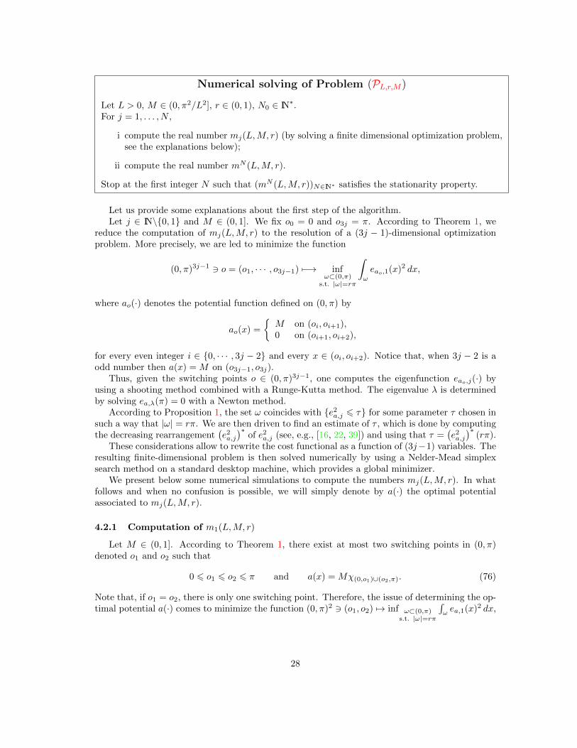
Numerical solving of Problem (PL,r,M)
Let L > 0, M ∈ (0, π2/L2], r ∈ (0, 1), N0 ∈ IN∗.For j = 1, . . . , N ,
i compute the real number mj(L,M, r) (by solving a finite dimensional optimization problem,see the explanations below);
ii compute the real number mN (L,M, r).
Stop at the first integer N such that (mN (L,M, r))N∈IN∗ satisfies the stationarity property.
Let us provide some explanations about the first step of the algorithm.Let j ∈ IN\0, 1 and M ∈ (0, 1]. We fix o0 = 0 and o3j = π. According to Theorem 1, we
reduce the computation of mj(L,M, r) to the resolution of a (3j − 1)-dimensional optimizationproblem. More precisely, we are led to minimize the function
(0, π)3j−1 3 o = (o1, · · · , o3j−1) 7−→ infω⊂(0,π)
s.t. |ω|=rπ
∫
ω
eao,1(x)2 dx,
where ao(·) denotes the potential function defined on (0, π) by
ao(x) =
M on (oi, oi+1),0 on (oi+1, oi+2),
for every even integer i ∈ 0, · · · , 3j − 2 and every x ∈ (oi, oi+2). Notice that, when 3j − 2 is aodd number then a(x) = M on (o3j−1, o3j).
Thus, given the switching points o ∈ (0, π)3j−1, one computes the eigenfunction eao,j(·) byusing a shooting method combined with a Runge-Kutta method. The eigenvalue λ is determinedby solving ea,λ(π) = 0 with a Newton method.
According to Proposition 1, the set ω coincides with e2a,j 6 τ for some parameter τ chosen in
such a way that |ω| = rπ. We are then driven to find an estimate of τ , which is done by computingthe decreasing rearrangement
(e2a,j
)∗of e2
a,j (see, e.g., [16, 22, 39]) and using that τ =(e2a,j
)∗(rπ).
These considerations allow to rewrite the cost functional as a function of (3j−1) variables. Theresulting finite-dimensional problem is then solved numerically by using a Nelder-Mead simplexsearch method on a standard desktop machine, which provides a global minimizer.
We present below some numerical simulations to compute the numbers mj(L,M, r). In whatfollows and when no confusion is possible, we will simply denote by a(·) the optimal potentialassociated to mj(L,M, r).
4.2.1 Computation of m1(L,M, r)
Let M ∈ (0, 1]. According to Theorem 1, there exist at most two switching points in (0, π)denoted o1 and o2 such that
0 6 o1 6 o2 6 π and a(x) = Mχ(0,o1)∪(o2,π). (76)
Note that, if o1 = o2, there is only one switching point. Therefore, the issue of determining the op-timal potential a(·) comes to minimize the function (0, π)2 3 (o1, o2) 7→ inf ω⊂(0,π)
s.t. |ω|=rπ
∫ωea,1(x)2 dx,
28

where a(·) is given by (76). Fixing τa =√λ2a,1 −M , one computes
ea,1(x) =
sin (τax) x ∈ (0, o1),sin (τao1) cos (λa,1(x− o1)) + τa
λa,1cos (τao1) sin (λa,1(x− o1)) x ∈ (o1, o2),
sin(τao1) cos(λa,1(o2−o1))+ τaλa,1
cos(τao1) sin(λa,1(o2−o1))
sin(τa(π−o2)) sin(τa(π − x)) x ∈ (o2, π),
up to a multiplicative normalization constant, where the eigenvalue λa,1 solves the transcendentalequation
λa,1τatan(τa(π − o2 + o1))
tan(λa,1(o2 − o1))− τ2
a = Msin(τa(π − o2)) sin(τao1)
cos(τa(π − o2 + o1)).
This last equation is solved numerically by using a Newton method. Since M ∈ (0, 1], the eigen-function ea,1 is concave on (0, π). As a consequence, the optimal set ω, as level set of the functione2a,1, writes ω = (0, α) ∪ (β, π) with α < β, according to Proposition 1. In that case, α and β are
determined with the help of a Newton method, using that β = (1−r)π+α and ea,1(α)2 = ea,1(β)2.The numerical results are gathered on Fig. 5.
0 1 2 3
0
0.2
0.4
0.6
0.8
1
α β
x
0 0.2 0.4 0.6 0.8 1
0
0.2
0.4
0.6
0.8
1
r
0 5 · 10−2 0.1 0.15 0.2
0
0.5
1
·10−2
r
Figure 5: Left: L = π and M = 1. Plots of the optimal set ω∗1(−), a∗1(-) and e2a∗1 ,1
(. . . ) w.r.t. thespace variable with r = 0.3. Middle and right: L = π and M = 1. Comparison of the numerical
results with the bounds obtained in Theorem 1: plots of r 7→ m1(π, 1, r) (—), r 7→ r− sin(πr)π (—)
and r 7→ r3/2 (−−−).
4.2.2 Computation of mj(L,M, r) for j > 2.
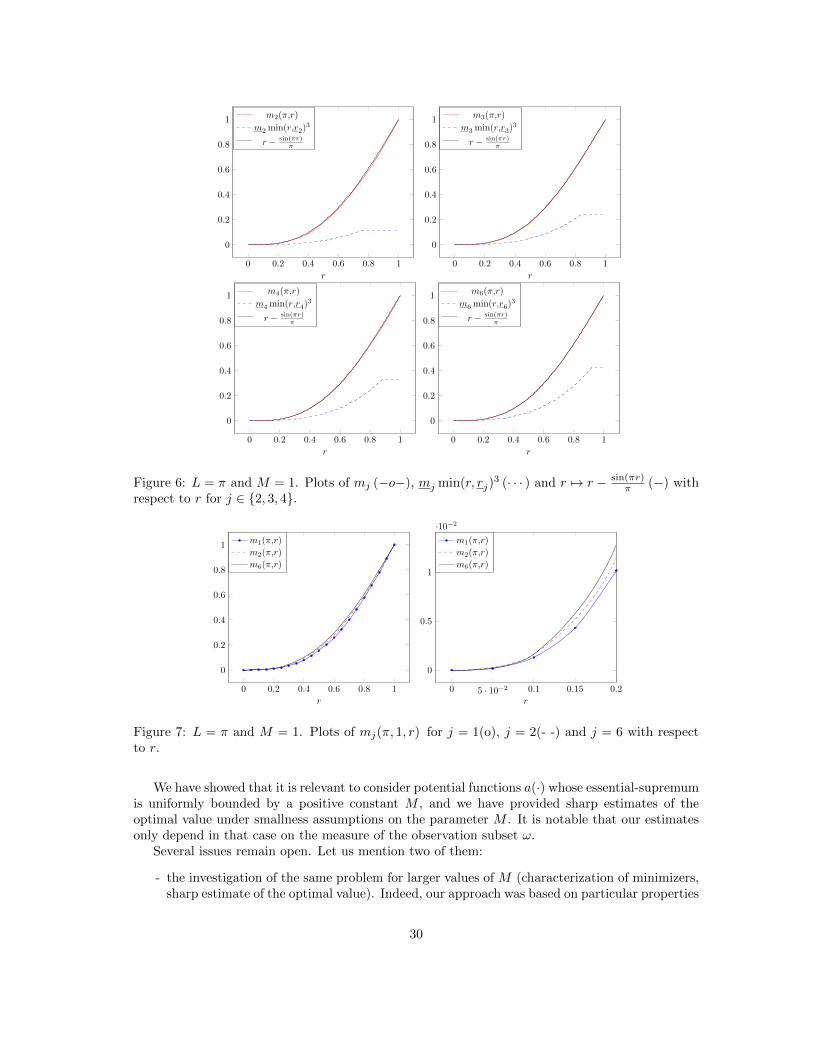
Figures 6 and 7 illustrate the cases j = 2, 3, 4. The parameters r and M are running overthe interval [0, 1]. On Figure 6, the optimal value of the criterion (w.r.t. r), obtained by using aNelder-Mead simplex search method, is compared to the estimate obtained in Theorem 4 for theparameter values j ∈ 2, 3, 4. Recall that the numbers mj are defined in Proposition 4. On Figure7, the graph of the optimal value with respect to r is plotted for the parameter values j ∈ 1, 2, 6.Notice that the mapping j 7→ mj(L,M, r) seems to be increasing, although we did not manage toprove it. This seems to indicate that the optimal index j0 introduced in Theorem 1 is equal to 1.
5 Concluding remarks
In this article, we have investigated the optimization problem (PL,r,M ) which allows to providea quantitative estimate of the “non-localization” property of Sturm-Liouville eigenfunctions relatedto the operator Aa defined by (1).
29
0 0.2 0.4 0.6 0.8 1
0
0.2
0.4
0.6
0.8
1
r
m2(π,r)
m2 min(r,r2)3
r − sin(πr)π
0 0.2 0.4 0.6 0.8 1
0
0.2
0.4
0.6
0.8
1
r
m3(π,r)
m3 min(r,r3)3
r − sin(πr)π
0 0.2 0.4 0.6 0.8 1
0
0.2
0.4
0.6
0.8
1
r
m4(π,r)
m4 min(r,r4)3
r − sin(πr)π
0 0.2 0.4 0.6 0.8 1
0
0.2
0.4
0.6
0.8
1
r
m6(π,r)
m6 min(r,r6)3
r − sin(πr)π
Figure 6: L = π and M = 1. Plots of mj (−o−), mj min(r, rj)3 (· · · ) and r 7→ r − sin(πr)
π (−) withrespect to r for j ∈ 2, 3, 4.
0 0.2 0.4 0.6 0.8 1
0
0.2
0.4
0.6
0.8
1
r
m1(π,r)
m2(π,r)
m6(π,r)
0 5 · 10−2 0.1 0.15 0.2
0
0.5
1
·10−2
r
m1(π,r)
m2(π,r)
m6(π,r)
Figure 7: L = π and M = 1. Plots of mj(π, 1, r) for j = 1(o), j = 2(- -) and j = 6 with respectto r.
We have showed that it is relevant to consider potential functions a(·) whose essential-supremumis uniformly bounded by a positive constant M , and we have provided sharp estimates of theoptimal value under smallness assumptions on the parameter M . It is notable that our estimatesonly depend in that case on the measure of the observation subset ω.
Several issues remain open. Let us mention two of them:
- the investigation of the same problem for larger values of M (characterization of minimizers,sharp estimate of the optimal value). Indeed, our approach was based on particular properties
30

of eigenfunctions holding only whenever M is small enough. Obtaining new estimates wouldrequire to develop a new approach.
- the development of efficient numerical methods to solve (PL,r,M ). On Fig. 8, we have plottedthe quantity mj(π,M, r), j = 1, 2, 3, 5 with respect to the parameter r, for several valuesof M greater than the critical value M = 1. These simulations drive us to formulate, aspreviously, the conjecture that the optimal index is j0 = 1. Note that the computation ofthese quantities need to solve optimization problems for which the objective function enjoysplenty of local minimizers. This is why we chose to solve this problem with the help of agenetic algorithm, quite efficient but very costly in terms of computing time, even for smallvalues of j.
0 0.2 0.4 0.6 0.8 1
0
0.2
0.4
0.6
0.8
1
r
m1(π,1,r)
m2(π,1,r)
m3(π,1,r)
m5(π,1,r)
0 0.2 0.4 0.6 0.8 1
0
0.2
0.4
0.6
0.8
1
r
m1(π,2,r)
m2(π,2,r)
m3(π,2,r)
m5(π,2,r)
0 0.2 0.4 0.6 0.8 1
0
0.2
0.4
0.6
0.8
1
r
m1(π,4,r)
m2(π,4,r)
m3(π,4,r)
m5(π,4,r)
0 5 · 10−2 0.1 0.15 0.2 0.25 0.3
0
1
2
3
4
·10−2
r
m1(π,1,r)
m2(π,1,r)
m3(π,1,r)
m5(π,1,r)
0 5 · 10−2 0.1 0.15 0.2 0.25 0.3
0
1
2
3
4
·10−2
r
m1(π,2,r)
m2(π,2,r)
m3(π,2,r)
m5(π,2,r)
0 5 · 10−2 0.1 0.15 0.2 0.25 0.3
0
1
2
3
4
·10−2
r
m1(π,4,r)
m2(π,4,r)
m3(π,4,r)
m5(π,4,r)
Figure 8: L = π. (Top) Plots of mj(π,M, r) w.r.t. r for M = 1, 2, 4. (Bottom) Zoom on theprevious plots around r = 0.
Appendix
A Proof of Lemma 4
Let us define φj =eaj,j(·)e′aj,j
(0) . The function φj solves the Cauchy system
−φ′′j (x) + aj(x)φj(x) = λ2a,jφj(x), x ∈ (0, L),
φj(0) = 0, φ′j(0) = 1.
Let us notice that, according to the Courant-Fischer minimax principle, there holds λaj ,j > πL
for every j ∈ IN∗ and limj→+∞ λaj ,j = +∞. According to [32, Chapter 1, Theorem 3] and using
31

a rescaling argument, we infer φj(x) =sin(λaj,jx)
λaj,j+ O
(1
λ2aj,j
). As a consequence, there holds
φ2j (x) =
sin2(λaj,jx)
λ2aj,j
+O
(1
λ3aj,j
), where the remainder term does not depend on x. Therefore, using
the Riemann-Lebesgue lemma, one gets that∫ L
0φ2j (x)dx = L
2λ2a,j
+o(
1λ2a,j
), and since eaj ,j =
φj‖φj‖2 ,
the combination of two last equalities yields
e2aj ,j(x) =
2
Lsin2(λaj ,jx) + O
(1
λaj ,j
). (77)
Let ϕ ∈ L1(0, L). Using (77), one shows that
∫ L
0
eaj ,j(x)2ϕ(x) dx =2
L
∫ β
α
sin2(λaj ,jx)ϕ(x) dx+ O
(1
λaj ,j
).
The expected result follows by linearizing sin2(λaj ,jx) and using the Riemann-Lebesgue lemma.
B Proofs of Lemmas 8 and 10
The proofs are based on the following Lemma.
Lemma 11. Let j ∈ IN∗ and i0 ∈ IN∗ such that i0 6 j − 1. Define
g(i0, j) =j − i0√j2 + 1
+1√j2 + 1
(j2−2j2
) i02 − 1
1−(
j2
j2−2
) 12
.
There holds
g(i0, j) > rj :=
(j +
√j2 − 2
2√j2 + 1
)(j − (j2 − 2)
j2
jj−1
).
Proof. Let γ : IN\0, 1 3 j 7→(
j2
j2−2
). Notice that γ(j) ∈ (1, 2) for every j ∈ IN\0, 1. The
derivative of g with respect to i0 writes
∂i0g(i0, j) =−(
1γ(j)
) i02
ln( 1γ(j) ) + 2(
√γ(j)− 1)
2√j2 + 1
(√γ(j)− 1
) 6 0,
and therefore
g(i0, j) > g(j − 1, j) =
√γ(j)(γ(j)
j2 − 1)√
j2 + 1(√γ(j)− 1)γ(j)
j2
.
Straightforward computations show that
√γ(j)(γ(j)
j2 − 1)√
j2 + 1(√γ(j)− 1)γ(j)
j2
=
(j +
√j2 − 2
2√j2 + 1
)(j − (j2 − 2)
j2
jj−1
),
which concludes the proof.
32

Proof of Lemma 8. In the sequel we will use the notations in (46), the definition of Ai in (53)and the definition of ∆j in (54).
From (53) and 1√j2+1
6 ηi 6 1√j2−1
, we notice that
Ai+1
Ai=
(1− η2i )η2
i+1
(1 + η2i+1)η2
i
6 1
Let i0 ∈ 1, · · · , j − 1 such that for every i 6 i0 − 1, τ < Ai and for every i > i0, τ > Ai (seeFigure ?? with j = 4 and i0 = 2). By definition of ω, one has
|ω| = |∆j(x)2 < τ| > |ωi0 |
with ωi0 = ∆j(·)2 6 Ai0. Let us denote by ri0 ∈ (0, 1) the real number defined by ri0 =|∆j(·)26Ai0|
L . Note that there holds obviously r > ri0 .
Let us now find a lower bound estimate of ri0 . Let i ∈ 0, · · · , j−1 and let ωi0i = ωi0∩(xij , xi+1j ).
There exist αi0i , βi0i and ri ∈ [0, 1] such that ωi0i = (xij , αi0i )∪ (βi0i , x
i+1j ), |ωi0i | = ri(x
i+1j −xij), and
therefore∑j−1i=0 ri(x
i+1j − xij) = ri0L.
By definition of ωi0 one has ∆j(αi0i ) = ∆j(β
i0i ) =
√Ai0 , for every i 6 i0−1 and ωi0i = (xij , x
i+1j )
for every i > i0. Consequently there holds
αi0i =
√Ai0Ai
(ximax − xij) + xij , βi0i = xi+1j −
√Ai0Ai
(xi+1j − ximax).
for all i 6 i0 − 1. As a result, one gets
ri0L =∑i0−1i=0 (αi0i − xij + xi+1
j − βi0i ) + (L− xi0) =∑i0−1i=0
√Ai0Ai
(xi+1j − xij) + (L− xi0).
Dividing by L, we have
ri0 =
i0−1∑
i=0
√Ai0Ai
ηi +
j−1∑
i=i0
ηi, (78)
where the numbers ηi are defined by (46).This last expression also rewrites
ri0 = ηi0
i0−1∑
i=0
√√√√i0∏
k=i+1
(1− η2
k−1
1 + η2k
)+
j−1∑
i=i0
ηi,
in terms of the real numbers ηi. Since 1√j2+1
6 ηi 6 1√j2−1
for every j ∈ IN∗ and i ∈ 0, · · · , j−1,one infers that
ri0 > ηi0∑i0−1i=0
(j2−2j2
) i0−i2
+∑j−1i=i0
ηi > g(i0, j),
with
g : (i0, j) 7→j − i0√j2 + 1
+1√j2 + 1
(j2−2j2
) i02 − 1
1−(
j2
j2−2
) 12
By Lemma 11, we conclude that for every i0 > 1, r >
(j+√j2−2
2√j2+1
)(j − (j2−2)
j2
jj−1
). As a result, if
r <
(j+√j2−2
2√j2+1
)(j − (j2−2)
j2
jj−1
), one has τ 6 Ai for every i ∈ 0, · · · , j − 1.
33

Proof of Lemma 10. In the sequel we will use the notations in (46) and the definition of ∆j in(54) where A1 is defined in (68), A0 is defined in (69) and for all i ∈ 2, · · · , j − 1 Ai is definedin (70) .
Let i0 ∈ 1, · · · , j − 1 and let us introduce the sets
Ik = i ∈ 0, · · · , j − 1 such thatAi > Ak and Jk = i ∈ 0, · · · , j − 1 such thatAi 6 Ak.
From (68), (69), (70) and 1√j2+1
6 ηi 6 1√j2−1
, we notice that
Ai+1
Ai=
(1− η2i )η2
i+1
(1 + η2i+1)η2
i
6 1, for all i ∈ 1, · · · , j − 1 andA0
A16 1. (79)
Case 1: 0 ∈ Ji0 . Thanks to (79), one has Ji0 = 0, i0 + 1, · · · , j − 1. By mimicking the proof ofLemma 8 (notably the equality (78)), we have
r =
i0∑
i=1
√Ai0+1
Aiηi +
∑
i∈Ji0
ηi > ηi0
i0∑
i=1
√√√√i0+1∏
k=i+1
(1− η2
k−1
1 + η2k
)+
j−1∑
i=i0+1
ηi + η0,
> ηi0
i0∑
i=1
(j2 − 2
j2
) i0+1−i2
+
j−1∑
i=i0+1
ηi + η0 > g(i0, j),
with g : (i0, j) 7→ j−i0√j2+1
+ 1√j2+1
(j2−2
j2
) i02 −1
1−(
j2
j2−2
) 12
, which leads to the desired conclusion using
Lemma 11.
Case 2: 0 ∈ Ii0 . Thanks to (79), one has Ji0 = i0, · · · , j − 1. By mimicking the proof of Lemma8, we have
ri0 =
√Ai0A0
η0 +
i0−1∑
i=1
√Ai0Ai
ηi +
j−1∑
i=i0
ηi
Thanks to (69), (70) and 1√j2+1
6 ηi 6 1√j2−1
,
√Ai0A0
η0 > ηi0
√(j2 + 2)(j2 − 1)
j2(j2 + 1)
(j2
j2 − 2
) i0−22
and
√Ai0Ai
ηi > ηi0
(j2 − 2
j2
) i0−i2
.
Since the inequality (j2+2)(j2−1)j2(j2+1) >
(j2
j2−2
)2
is true for every j > 1, we thus infer
ri0 > ηi0
i0−1∑
i=0
(j2 − 2
j2
) i0−i2
+
j−1∑
i=i0
ηi > g(i0, j).
By using Lemma 11, we conclude the proof.
C Proof of Theorem 3
Before proving this theorem, let us recall some basic facts on Ingham’s inequality (see [17]), aninequality for nonharmonic Fourier series much used in control theory.
34
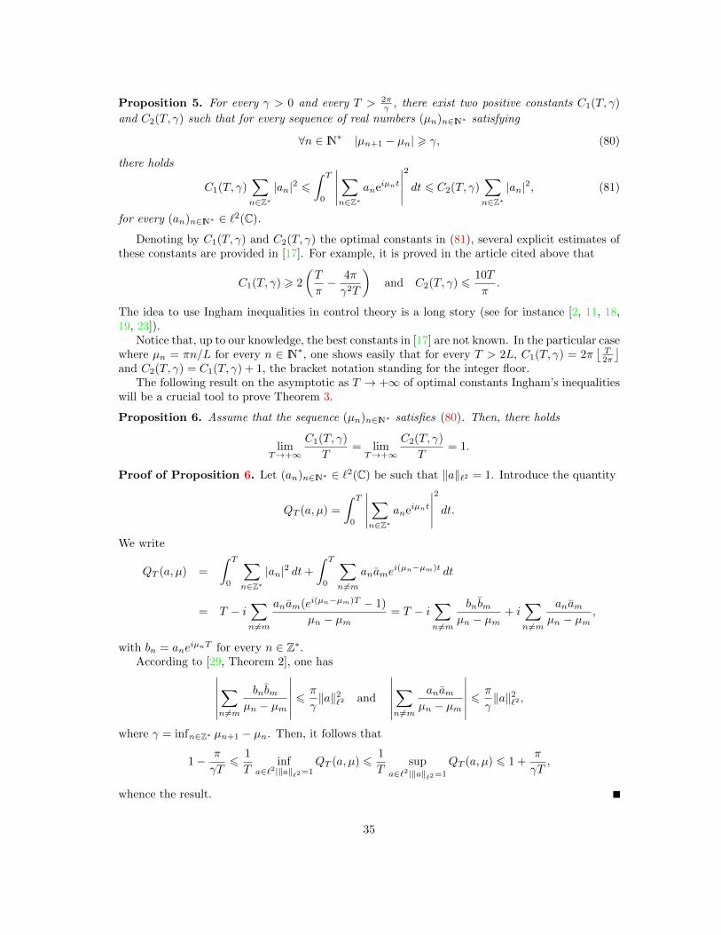
Proposition 5. For every γ > 0 and every T > 2πγ , there exist two positive constants C1(T, γ)
and C2(T, γ) such that for every sequence of real numbers (µn)n∈IN∗ satisfying
∀n ∈ IN∗ |µn+1 − µn| > γ, (80)
there holds
C1(T, γ)∑
n∈Z∗|an|2 6
∫ T
0
∣∣∣∣∣∑
n∈Z∗aneiµnt
∣∣∣∣∣
2
dt 6 C2(T, γ)∑
n∈Z∗|an|2, (81)
for every (an)n∈IN∗ ∈ `2(C).
Denoting by C1(T, γ) and C2(T, γ) the optimal constants in (81), several explicit estimates ofthese constants are provided in [17]. For example, it is proved in the article cited above that
C1(T, γ) > 2
(T
π− 4π
γ2T
)and C2(T, γ) 6
10T
π.
The idea to use Ingham inequalities in control theory is a long story (see for instance [2, 11, 18,19, 23]).
Notice that, up to our knowledge, the best constants in [17] are not known. In the particular casewhere µn = πn/L for every n ∈ IN∗, one shows easily that for every T > 2L, C1(T, γ) = 2π
⌊T2π
⌋
and C2(T, γ) = C1(T, γ) + 1, the bracket notation standing for the integer floor.The following result on the asymptotic as T → +∞ of optimal constants Ingham’s inequalities
will be a crucial tool to prove Theorem 3.
Proposition 6. Assume that the sequence (µn)n∈IN∗ satisfies (80). Then, there holds
limT→+∞
C1(T, γ)
T= limT→+∞
C2(T, γ)
T= 1.
Proof of Proposition 6. Let (an)n∈IN∗ ∈ `2(C) be such that ‖a‖`2 = 1. Introduce the quantity
QT (a, µ) =
∫ T
0
∣∣∣∣∣∑
n∈Z∗aneiµnt
∣∣∣∣∣
2
dt.
We write
QT (a, µ) =
∫ T
0
∑
n∈Z∗|an|2 dt+
∫ T
0
∑
n 6=maname
i(µn−µm)t dt
= T − i∑
n 6=m
anam(ei(µn−µm)T − 1)
µn − µm= T − i
∑
n 6=m
bnbmµn − µm
+ i∑
n 6=m
anamµn − µm
,
with bn = aneiµnT for every n ∈ Z∗.
According to [29, Theorem 2], one has∣∣∣∣∣∣∑
n 6=m
bnbmµn − µm
∣∣∣∣∣∣6π
γ‖a‖2`2 and
∣∣∣∣∣∣∑
n 6=m
anamµn − µm
∣∣∣∣∣∣6π
γ‖a‖2`2 ,
where γ = infn∈Z∗ µn+1 − µn. Then, it follows that
1− π
γT6
1
Tinf
a∈`2|‖a‖`2=1QT (a, µ) 6
1
Tsup
a∈`2|‖a‖`2=1
QT (a, µ) 6 1 +π
γT,
whence the result.
35
Decomposing the solution ϕ of (71) in the spectral basis ea,jj∈IN∗ allows to write that
ϕ(t, x) =
+∞∑
j=1
(αj cos(λa,jt) + βj sin(λa,jt)) ea,j(x), (82)
where
αj =
∫ L
0
ϕ0(x)ea,j(x) dx, βj =1
λa,j
∫ L
0
ϕ1(x)ea,j(x) dx, (83)
for every j ∈ IN∗. We are now ready to prove Theorem 3.
Proof of Theorem 3. Introduce the spectral gap γ = infj∈N∗ λa,j+1 − λa,j . It is well-knownthat γ > 0 for every a ∈ L∞(0, L). Let us first prove point (i). Using (81), one has for T > 2π/γ,
∫ T
0
∫
ω
|∂tϕ(t, x)|2 dxdt =1
4
∫ T
0
∫
ω
∣∣∣∣∣∑
k∈Z∗i sgn(k)λa,|k|
√α2|k| + β2
|k|ei sgn(k)(λa,|k|t−θ|k|)ea,|k|(x)
∣∣∣∣∣
2
dxdt
>C1(T, γ)
4
∑
k∈Z∗(α2|k| + β2
|k|)λ2a,|k|
∫
ω
ea,|k|(x)2 dx
=C1(T, γ)
2
+∞∑
j=1
(α2j + β2
j )λ2a,j
∫
ω
ea,j(x)2 dx, (84)
where (θj)j∈IN∗ denotes the sequence defined by eiθj =αj+iβj√α2j+β
2j
for every j ∈ IN∗. Combining the
energy identity
∫ L
0
(ϕ2t (t, x) + ϕ2
x(t, x) + a(x)ϕ2(t, x))dx =
+∞∑
j=1
λ2a,j(α
2j + β2
j ), (85)
with (73), (82), (83) and (85), one gets
CT,obs(ω) = inf(λa,jαj ,λa,jβj)∈l2(IR)2
∫ T0
∫ω|∑+∞
j=1 (−λa,jαj sin(λa,jt) + λa,jβj cos(λa,jt)) ea,j(x)|2 dxdt∑+∞j=1 λ
2a,j(α
2j + β2
j ),
(86)According to (84), it follows that
CT,obs(ω) >C1(T, γ)
2infj∈IN∗
∫
ω
ea,j(x)2 dx. (87)
Taking now αj = (δkj)k∈IN∗ and βj = (δk′j)k′∈IN∗ in (86) where δkj denotes the Kronecker delta,we obtain
CT,obs(ω) 6T
2infj∈IN∗
∫
ω
ea,j(x)2 dx. (88)
Combining (87), (88) with the asymptotic of optimal constant C1(T, γ) in Ingham’s inequalitiesstated in Proposition 6 leads to the desired result. Let us now prove point ii. According to (85),(87) and (88), there holds
0 <C1(T, γ)
26
CT,obs(ω)
infj∈IN∗∫ωea,j(x)2 dx
6T
2(89)
with C1(T, γ) > 2(Tπ − 4π
γ2T
). To conclude, it remains to provide an estimate of the spectral gap
γ.
36
Lemma 12. Let a ∈ AM (0, L) with M ∈ (0, 3π2/L2). There holds
∀j ∈ IN∗, λa,j+1 − λa,j >3π2
L2 −M2πL +
√π2
L2 +M.
Proof. The Courant-Fischer minimax principle writes
λ2a,j = min
V⊂H10 (0,π)
dimV=j
maxu∈V \0
∫ π0
(u′(x)2 + a(x)u(x)2)dx∫ π0u(x)2 dx
. (90)
Using that 0 6 a(x) 6 M for almost every x ∈ (0, L) yields jπL 6 λa,j 6
√(jπL
)2+M , for every
j ∈ IN∗. It suffices indeed to compare λ2a,j with the j-th eigenvalue of a Sturm-Liouville operator
with constant coefficients. We infer
λa,j+1 − λa,j >(j + 1)π
L−√(
jπ
L
)2
+M =(1 + 2j) π
2
L2 −M
(j + 1) πL +
√(j2π2
L2
)+M
for every j ∈ IN∗. The sequence j 7→ (1+2j) π2
L2−M
(j+1) πL+
√(j2π2
L2
)+M
being increasing, the expected estimate
follows.
Therefore, according to Lemma 12, one has γ > γM . Hence, choosing γ = γM in (89) for allT > T (M) = 2π
γMyields the expected conclusion.
References[1] Nalini Anantharaman and Stephane Nonnenmacher, Half-delocalization of eigenfunctions for the Laplacian on
an Anosov manifold, Ann. Inst. Four. (Grenoble), 57 (2007), no. 7, 2465–2523.
[2] John M. Ball and Marshall Slemrod, Nonharmonic Fourier series and the stabilization of distributed semilinearcontrol systems, Comm. Pure Appl. Math. 32 (1979), no. 4, 555–587.
[3] Nicolas Burq and Maciej Zworski, Bouncing ball modes and Quantum chaos, SIAM Rev., 47 (2005), no. 1,43–49.
[4] Yves Colin de Verdiere, Ergodicite et fonctions propres du Laplacien, Comm. Math. Phys. 102 (1985), 497–502.
[5] Jean-Michel Coron, Control and nonlinearity, Volume 136 of Mathematical Surveys and Monographs. AmericanMathematical Society, Providence (2007).
[6] Steven Cox and Enrique Zuazua, The rate at which energy decays in a damped string, Comm. in partialdifferential equations 19, (1994), 213–243.
[7] Thomas Duyckaerts, Xu Zhang and Enrique Zuazua, On the optimality of the observability inequalities forparabolic and hyperbolic systems with potentials, Ann. Inst. H. Poincare Anal. Non Lineaire 25 (2008), 1–41.
[8] Lawrence C. Evans, Partial Differential Equations, Graduate Studies in Mathematics, 19, AMS (1998).
[9] Patrick Gerard and Eric Leichtnam, Ergodic properties of eigenfunctions for the Dirichlet problem, Duke Math.J., 71 (1993), 559-607.
[10] Denis Grebenkov and Binh T. Nguyen Geometrical structure of Laplacian eigenfunctions, SIAM Rev. 55(2013), no. 4, 601–667.
[11] Alain Haraux, Series lacunaires et controle semi-interne des vibrations d’une plaque rectangulaire. (French.English summary) [Lacunary series and semi-internal control of the vibrations of a rectangular plate], J. Math.Pures Appl. (9) 68 (1989), no. 4, 457–465 (1990).
[12] Alain Haraux, Thibault Liard and Yannick Privat, How to estimate observability constants of one-dimensionalwave equations? Propagation versus Spectral methods, To appear in J. Evol. Eq.
37

[13] Andrew Hassell and Steve Zelditch, Quantum ergodicity of boundary values of eigenfunctions, Comm. Math.Phys. 248 (2004), no. 1, 119–168.
[14] Pascal Hebrard and Antoine Henrot, Optimal shape and position of the actuators for the stabilization of astring, Syst. Cont. Letters 48 (2003), 199–209.
[15] Antoine Henrot, Extremum problems for eigenvalues of elliptic operators, Frontiers in Mathematics, BirkhauserVerlag, Basel, 2006.
[16] Antoine Henrot and Michel Pierre, Variation et optimisation de formes (French) [Shape variation and opti-mization] Une analyse geometrique. [A geometric analysis], Math. & Appl. 48, Springer, Berlin, 2005.
[17] Albert E. Ingham, Some trigonometrical inequalities with applications to the theory of series, Math. Zeitschrift41 (1936), 367–379.
[18] Stephane Jaffard and Sorin Micu, Estimates of the constants in generalized Ingham’s inequality and applicationsto the control of the wave equation, Asymptot. Anal. 28 (2001), no. 3-4, 181–214.
[19] Stephane Jaffard, Marius Tucsnak and Enrique Zuazua, On a theorem of Ingham, J. Fourier Anal. Appl. 3(1997), 577–582.
[20] Dmitry Jakobson and Steve Zelditch, Classical limits of eigenfunctions for some completely integrable systems,Emerging applications of number theory (Minneapolis, MN, 1996), 329–354, IMA Vol. Math. Appl., 109,Springer, New York, 1999.
[21] Tosio Kato, Perturbation theory for linear operators, Classics in Mathematics. Springer-Verlag, Berlin, 1995.
[22] Bernd Kawohl, rearrangements and convexity of level sets in PDE, Springer Lecture Notes in Math. 1150,(1985), 1–134.
[23] Vilmos Komornik and Paola Loreti, Fourier Series in Control Theory, Springer-Verlag, New York, 2005.
[24] Vilmos Komornik and Bernadette Miara, Cross-like internal observability of rectangular membranes, EvolutionEqu. Control Theory 3 (2014), no.1, 135–146.
[25] John Lagnese, Control of wave processes with distributed controls supported on a subregion, SIAM J. ControlOptim. (1983)
[26] Tony Lassila, Optimal damping of a membrane and topological shape optimization, Struct. Multidiscip. Optim.38 (2009), no. 1, 43?52.
[27] Xunjing Li and Jiongmin Yong, Necessary conditions for optimal control of distributed parameter systems,SIAM J. Control Optim. 29 (1991), no. 4, 895–908.
[28] Jacques-Louis Lions, Controlabilite exacte, perturbations et stabilisation de systemes distribues, Tomes 1 & 2,Rech. Math. Appl. [Research in Applied Mathematics], Masson (1988).
[29] Hugh L. Montgomery and Robert C. Vaughan, Hilbert’s inequality, J. London Math. Soc. 2 (1974), no. 8,73–82.
[30] Arnaud Munch, Pablo Pedregal and Francisco Periago Optimal design of the damping set for the stabilizationof the wave equation, J. Differential Equations 231 (2006), no. 1, 331–358.
[31] Francisco Periago, Optimal shape and position of the support for the internal exact control of a string, Syst.Cont. Letters 58 (2009), no. 2, 136–140.
[32] Jurgen Poschel, Eugene Trubowitz Inverse spectral theory, Academic Press Orlando, 1987.
[33] Yannick Privat, Emmanuel Trelat and Enrique Zuazua, Optimal observability of the multi-dimensional waveand Schrodinger equations in quantum ergodic domains, J. Eur. Math. Soc. (JEMS) 18 (2016), no. 5, 1043?1111.
[34] Yannick Privat, Emmanuel Trelat and Enrique Zuazua, Complexity and regularity of optimal observationdomains for the wave equation with fixed initial data, Discrete Cont. Dynam. Syst. 35 (2015), no. 12, 6133–6153.
[35] Yannick Privat, Emmanuel Trelat and Enrique Zuazua, Optimal location of controllers for the one-dimensionalwave equation, Ann. Inst. H. Poincare Anal. Non Lineaire 30 (2013), 1097–1126.
[36] Yannick Privat, Emmanuel Trelat and Enrique Zuazua, Optimal observation of the one-dimensional waveequation, J. Fourier Anal. Appl. 19 (2013), no. 3, 514–544.
[37] Yannick Privat, Emmanuel Trelat and Enrique Zuazua, Optimal shape and location of sensors for parabolicequations with random initial data, Arch. Ration. Mech. Anal., 216 (2015), 921–981.
[38] Yannick Privat, Emmanuel Trelat and Enrique Zuazua, Randomised observation, control and stabilisation ofwaves, ZAMM Z. Angew. Math. Mech. 96 (2016), no. 5, 538?549.
[39] Jean-Michel Rakotoson, Rearrangement relatif, Vol. 64 of Math. & Appl. (Berlin) [Mathematics & Applica-tions]. Springer, Berlin, 2008.
[40] Alexander I. Shnirelman, Ergodic properties of eigenfunctions, Uspenski Math. Nauk 29/6 (1974), 181–182.
[41] Enrique Zuazua, Exact controllability for semilinear wave equations in one space dimension, Ann. Inst. H.Poincare Anal. Non Lineaire 10 (1993), 109–129.
38