Non-linear vibration of hyperelastic axisymmetric solids by a mixed p-type method

International Journal of Non-Linear Mechanics 47 (2012) 30–41

Contents lists available at SciVerse ScienceDirect

International Journal of Non-Linear Mechanics

0020-74

doi:10.1

n Corr

E-m

tanveer

journal homepage: www.elsevier.com/locate/nlm

Non-linear vibration of hyperelastic axisymmetric solidsby a mixed p-type method

Muhammad Tanveer n, Jean W. Zu

Department of Mechanical and Industrial Engineering, University of Toronto, 5 King’s College Road, Toronto, Ontario, Canada M5S 3G8

a r t i c l e i n f o

Article history:

Received 31 March 2010

Received in revised form

4 July 2011

Accepted 3 August 2011Available online 29 September 2011

Keywords:

Axisymmetric solids

Hyperelastic materials

Mixed p-type formulation

Non-linear vibration

Polynomials

62/$ - see front matter & 2012 Published by

016/j.ijnonlinmec.2011.08.003

esponding author. Tel.: þ1 416 946 3709; fax

ail addresses: [email protected],

@mie.utoronto.ca (M. Tanveer).

a b s t r a c t

This paper presents finite amplitude transient vibration analysis of nearly incompressible hyperelastic

axisymmetric solids by a mixed p-type method. In this method, displacement and pressure fields are

separately defined using high degree polynomials and the solution is obtained with one or a few

elements depending upon the nature of the problem. Geometry of the element is defined by

polynomials of degrees much lower than that of displacement fields. The degrees of polynomials for

pressure fields are lower than those used for displacement fields.

Hyperelastic material is modelled by the Mooney–Rivlin material description. The total Lagrangian

formulation is utilized to describe the deformations of axisymmetric solids subjected to pressure loads.

Equations of motion are derived using the principle of virtual work and solved by the Newmark’s

method along with the Newton–Raphson iterative technique. The present formulation also includes the

asymmetric tangent load matrix, resulting in linearization of deformation dependent load, which

greatly reduces the number of equilibrium iterations to get the convergence of results at large strains.

A convergence study of the results is presented with respect to the degrees of polynomials for

displacement and pressure fields. The present method is verified by successfully comparing the results

with those from finite element method using the commercial software ANSYS. The numerical

simulations are conducted on circular plate, solid cylinder and spherical shells subjected to time

dependent pressure loads and the highly non-linear behaviour of hyperelastic solids undergoing finite

amplitude vibrations is studied. The method, presented herein, is very efficient, locking free, and

accurate, which does not require a large number of elements or the total degrees of freedom as it is

required in conventional finite element method for the convergence of results.

& 2012 Published by Elsevier Ltd.

1. Introduction

Hyperelastic materials are quite common in many engineeringapplications. These materials are incompressible or almostincompressible and undergo large strains when subjected toloads. In the last six decades, many constitutive models [1–3]are developed for hyperelastic materials, which can be used incomputational model according to the application. Nevertheless,computational modelling poses challenges owing to incompres-sibility. For example, the displacement based finite elementmethods, which are widely used for various applications andmaterials, are not efficient for almost incompressible materials [4].The common problems with these methods, when Poisson’s ratioapproaches 0.5, are the incorrect stresses, the ill conditioning ofstiffness matrix, and the locking. A huge amount of work has been

Elsevier Ltd.

: þ1 416 978 7753.

done by many researchers in the past to deal with the problemsdue to the condition of incompressibility in solids. A comprehen-sive survey on the finite element methods of incompressibleor almost incompressible materials can be found in papers byGadala [5], Sussman and Bathe [6] and Mackerle [7,8]. In thepresent work, only the most relevant papers are briefly discussed.

A great deal of research work has been devoted to the mixedvariational finite element methods for the analysis of incompres-sible and almost incompressible materials. In the mixed method,the displacements and the stresses (or hydrostatic pressures) areseparately defined and are subject to variation. In the mid 1960,Herrmann [9] published first paper on the mixed variationalmethod for incompressible and almost incompressible isotropicmaterials, where, in addition to displacements, mean-stresseswere separately interpolated. The analysis of orthotropic materi-als based on the same approach was later presented by Tayloret al. [10] and Key [11]. The work by Key [11] was also applicableto non-linear analysis. Following this, many papers were pub-lished on the non-linear analysis. Oden and Key [12] wrote apaper on the non-linear analysis of axisymmetric rubber solids.

www.elsevier.com/locate/nlm

www.elsevier.com/locate/nlm

dx.doi.org/10.1016/j.ijnonlinmec.2011.08.003

mailto:[email protected]

mailto:[email protected]

dx.doi.org/10.1016/j.ijnonlinmec.2011.08.003

1

2 3

4

5

6

7

8

9

10

11

12

Z

R

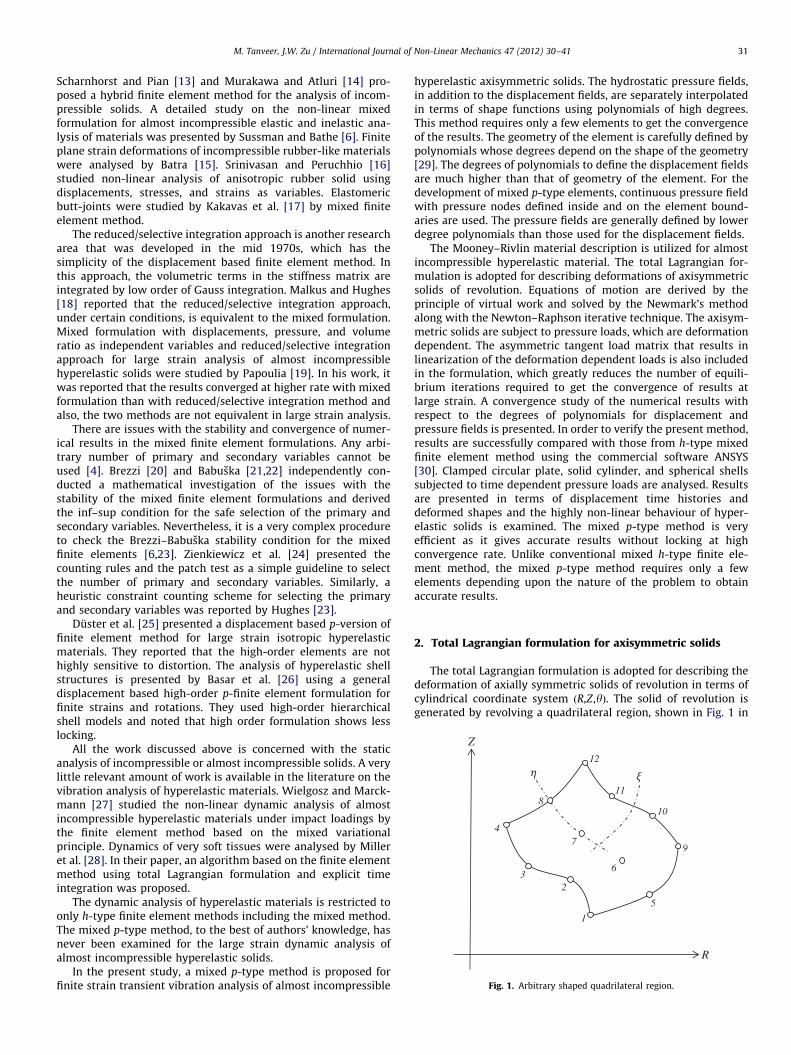
Fig. 1. Arbitrary shaped quadrilateral region.

M. Tanveer, J.W. Zu / International Journal of Non-Linear Mechanics 47 (2012) 30–41 31

Scharnhorst and Pian [13] and Murakawa and Atluri [14] pro-posed a hybrid finite element method for the analysis of incom-pressible solids. A detailed study on the non-linear mixedformulation for almost incompressible elastic and inelastic ana-lysis of materials was presented by Sussman and Bathe [6]. Finiteplane strain deformations of incompressible rubber-like materialswere analysed by Batra [15]. Srinivasan and Peruchhio [16]studied non-linear analysis of anisotropic rubber solid usingdisplacements, stresses, and strains as variables. Elastomericbutt-joints were studied by Kakavas et al. [17] by mixed finiteelement method.

The reduced/selective integration approach is another researcharea that was developed in the mid 1970s, which has thesimplicity of the displacement based finite element method. Inthis approach, the volumetric terms in the stiffness matrix areintegrated by low order of Gauss integration. Malkus and Hughes[18] reported that the reduced/selective integration approach,under certain conditions, is equivalent to the mixed formulation.Mixed formulation with displacements, pressure, and volumeratio as independent variables and reduced/selective integrationapproach for large strain analysis of almost incompressiblehyperelastic solids were studied by Papoulia [19]. In his work, itwas reported that the results converged at higher rate with mixedformulation than with reduced/selective integration method andalso, the two methods are not equivalent in large strain analysis.

There are issues with the stability and convergence of numer-ical results in the mixed finite element formulations. Any arbi-trary number of primary and secondary variables cannot beused [4]. Brezzi [20] and Babuska [21,22] independently con-ducted a mathematical investigation of the issues with thestability of the mixed finite element formulations and derivedthe inf–sup condition for the safe selection of the primary andsecondary variables. Nevertheless, it is a very complex procedureto check the Brezzi–Babuska stability condition for the mixedfinite elements [6,23]. Zienkiewicz et al. [24] presented thecounting rules and the patch test as a simple guideline to selectthe number of primary and secondary variables. Similarly, aheuristic constraint counting scheme for selecting the primaryand secondary variables was reported by Hughes [23].

Duster et al. [25] presented a displacement based p-version offinite element method for large strain isotropic hyperelasticmaterials. They reported that the high-order elements are nothighly sensitive to distortion. The analysis of hyperelastic shellstructures is presented by Basar et al. [26] using a generaldisplacement based high-order p-finite element formulation forfinite strains and rotations. They used high-order hierarchicalshell models and noted that high order formulation shows lesslocking.

All the work discussed above is concerned with the staticanalysis of incompressible or almost incompressible solids. A verylittle relevant amount of work is available in the literature on thevibration analysis of hyperelastic materials. Wielgosz and Marck-mann [27] studied the non-linear dynamic analysis of almostincompressible hyperelastic materials under impact loadings bythe finite element method based on the mixed variationalprinciple. Dynamics of very soft tissues were analysed by Milleret al. [28]. In their paper, an algorithm based on the finite elementmethod using total Lagrangian formulation and explicit timeintegration was proposed.

The dynamic analysis of hyperelastic materials is restricted toonly h-type finite element methods including the mixed method.The mixed p-type method, to the best of authors’ knowledge, hasnever been examined for the large strain dynamic analysis ofalmost incompressible hyperelastic solids.

In the present study, a mixed p-type method is proposed forfinite strain transient vibration analysis of almost incompressible

hyperelastic axisymmetric solids. The hydrostatic pressure fields,in addition to the displacement fields, are separately interpolatedin terms of shape functions using polynomials of high degrees.This method requires only a few elements to get the convergenceof the results. The geometry of the element is carefully defined bypolynomials whose degrees depend on the shape of the geometry[29]. The degrees of polynomials to define the displacement fieldsare much higher than that of geometry of the element. For thedevelopment of mixed p-type elements, continuous pressure fieldwith pressure nodes defined inside and on the element bound-aries are used. The pressure fields are generally defined by lowerdegree polynomials than those used for the displacement fields.

The Mooney–Rivlin material description is utilized for almostincompressible hyperelastic material. The total Lagrangian for-mulation is adopted for describing deformations of axisymmetricsolids of revolution. Equations of motion are derived by theprinciple of virtual work and solved by the Newmark’s methodalong with the Newton–Raphson iterative technique. The axisym-metric solids are subject to pressure loads, which are deformationdependent. The asymmetric tangent load matrix that results inlinearization of the deformation dependent loads is also includedin the formulation, which greatly reduces the number of equili-brium iterations required to get the convergence of results atlarge strain. A convergence study of the numerical results withrespect to the degrees of polynomials for displacement andpressure fields is presented. In order to verify the present method,results are successfully compared with those from h-type mixedfinite element method using the commercial software ANSYS[30]. Clamped circular plate, solid cylinder, and spherical shellssubjected to time dependent pressure loads are analysed. Resultsare presented in terms of displacement time histories anddeformed shapes and the highly non-linear behaviour of hyper-elastic solids is examined. The mixed p-type method is veryefficient as it gives accurate results without locking at highconvergence rate. Unlike conventional mixed h-type finite ele-ment method, the mixed p-type method requires only a fewelements depending upon the nature of the problem to obtainaccurate results.

2. Total Lagrangian formulation for axisymmetric solids

The total Lagrangian formulation is adopted for describing thedeformation of axially symmetric solids of revolution in terms ofcylindrical coordinate system ðR,Z,yÞ. The solid of revolution isgenerated by revolving a quadrilateral region, shown in Fig. 1 in

M. Tanveer, J.W. Zu / International Journal of Non-Linear Mechanics 47 (2012) 30–4132

R–Z plane, about z-axis. Material properties and geometry of solidare independent of circumferential direction y. With loading andboundary conditions as axisymmetric, three-dimensional pro-blem becomes two-dimensional and hence, the elastic equationsare defined using only the quadrilateral region shown in Fig. 1.During deformation, the position of a particle in R–Z plane at aninitial configuration 0 and a deformed configuration 1 are repre-sented by ðr0,z0Þ and (r, z) respectively. Taking into account thedisplacements, r and z can be further defined as

r¼ r0þv,

z¼ z0þw, ð1Þ

where v and w are the displacement components in R and Z

directions respectively.The Green–Lagrange strain matrix ½e� can be defined as

½e� ¼ 12ð½F�

T ½F��½I�Þ, ð2Þ

where [I] is the identity matrix and [F], defined below, is thedeformation gradient matrix:

½F� ¼

1þv,r0v,z0

0

w,r01þw,z0

0

0 0 1þ vr0

2664

3775: ð3Þ

In Eq. (3), v,r0¼ @v=@r0, v,z0

¼ @v=@z0, w,r0¼ @w=@r0, and w,z0

¼

@w=@z0. It is adopted in this paper that a comma as right subscriptdenotes the differentiation with respect to the coordinate follow-ing the comma.

The term [F]T[F] in Eq. (2) is the right Cauchy–Green deforma-tion matrix [C], which is expressed as

½C� ¼

ð1þv,r0Þ2þðw,r0

Þ2ð1þv,r0

Þv,z0þð1þw,z0

Þw,r00

ð1þw,z0Þ2þðv,z0

Þ2 0

Sym: ð1þ vr0Þ2

2664

3775:ð4Þ

The Voigt notation for Green–Lagrange strains from Eq. (2) can bedefined by

fegT ¼ ferr ezz eyy grzg, ð5Þ

where err ¼ v,r0þ1

2ðv2,r0þw2

,r0Þ, ezz ¼w,z0

þ12ðv

2,z0þw2

,z0Þ, eyy ¼ v=r0þ

12ðv=r0Þ

2, and grz ¼ 2erz ¼ v,z0þw,r0

þv,r0v,z0þw,r0

w,z0.

2.1. Hyperelastic material description

The Mooney–Rivlin material description for almost incom-pressible materials [31] is adopted to represent finite strainbehaviour of hyperelastic axisymmetric solids. The strain energyper unit undeformed volume of the material is expressed by

Wd ¼ C1ðI1�3ÞþC2ðI2�3Þþ12kðJ�1Þ2, ð6Þ

where C1 and C2 are the material constants, I1 and I2 are themodified invariants, J¼ detðFÞ is the volume ratio, and k is thebulk modulus. In Eq. (6), the quantities I1, I2, J, and k are

I1 ¼ I1I�1=33 , I2 ¼ I2I�2=3

3 , J¼ I1=23 , k¼

E

3ð1�2lÞ, ð7Þ

where E is Young’s modulus, l is Poisson’s ratio, and I1, I2 and I3

are the strain invariants, which are defined as

I1 ¼ CrrþCzzþCyy,

I2 ¼ CrrCzzþCrrCyyþCzzCyy�C2rz,

I3 ¼ CrrCzzCyy�C2rzCyy: ð8Þ

Note that for small strains, Young’s and shear moduli arerepresented by the values 6(C1þC2) and 2(C1þC2) respectively.

3. Mixed p-type formulation for hyperelastic materials

In Eq. (6), the strain energy density function is computed usingthe displacement fields only. In the mixed displacement/pressureformulation, the hydrostatic pressure is included as variables,which are separately interpolated. In order to include pressure inthe formulation as variables, the strain energy density function ismodified [4] and is given below.

W ¼WdþWp, ð9Þ

where Wp is the strain energy density function computed frompressures. Detailed information on the strain energy densityfunction in Eq. (9) can be found in [4,6]. The expression for Wp

is given below.

Wp ¼�1

2kðPd�pÞ2, ð10Þ

where p is the separately interpolated pressure and Pd is thepressure computed from displacement fields, which is expressed by

Pd ¼�kðJ�1Þ, ð11Þ

where the quantities k and J are already defined in Eq. (7).In this mixed displacement/pressure approach, the pressure Pd

is totally replaced by the pressure p. Therefore, any possibleinaccurate pressures computed from displacements are removedfrom stresses. Another advantage in this mixed formulation isthat if Wp is dropped from Eq. (9), the formulation becomes a puredisplacement based. Hence, the displacement based formulationis the special case of this mixed formulation.

A mixed p-type numerical formulation is developed basedon the mixed displacement/pressure approach and the detailsthereof are given in the following sections.

3.1. Geometry

In the mixed p-type formulation, problems are accuratelysolved by only one or a few elements depending upon theproblem. Convergence or the accuracy of numerical results isachieved by increasing the degree of polynomials of displacementand pressure fields, unlike conventional finite element method,where it is achieved by refining the mesh of isoparametric finiteelements. In the present method, simple geometric polynomialsare used for interpolation.

Geometry of the mixed p-type element is required to beaccurately defined [29]. Let us consider an arbitrarily shapedquadrilateral region, shown in Fig. 1 in R–Z plane, formed by fourcurved edges. In this figure, small circles on and inside theboundaries of the region represent the geometric nodes, whichare defined by their coordinates (Ri, Zi) with i¼1,2,3,y,s, where s

depends on the shape of the region. In Fig. 1, the value of s is 12,which is an arbitrary number. For example, only four geometricnodes can be used to accurately define a region formed by fourstraight edges. The coordinates (r0, z0) of an arbitrary point in theundeformed region, shown in Fig. 1, are interpolated by

r0 ¼Xs

i ¼ 1

Niðx,ZÞRi,

z0 ¼Xs

i ¼ 1

Niðx,ZÞZi, ð12Þ


where Niðx,ZÞ with i¼1,2,3,y,s are the geometric shape functions[32] in terms of natural coordinates x and Z, which are boundedby �1rðx,ZÞrþ1.

3.2. Displacement fields

The displacement fields are defined by polynomials of muchhigher degrees than those used for the geometry. With the inter-polation procedure defined above for the geometry, the displace-ment components v and w respectively in R and Z directions can beinterpolated with a different set of preselected nodal points on theregion shown in Fig. 1, which are defined by

v¼Xn

i ¼ 1

f iðx,ZÞVi,

w¼Xn

i ¼ 1

f iðx,ZÞWi, ð13Þ

where f iðx,ZÞ with i¼1,2,3,y,n are the displacement shapefunctions. In Eq. (13), the indices Vi and Wi are the degrees offreedom at the ith displacement node corresponding to v and w

respectively. In Eq. (13), n represents the number of displacementnodes and is defined by n¼ ðldþ1Þðmdþ1Þ, where ld and md

represent the degrees of polynomial in x and Z respectively.Using the relations given in Eqs. (12) and (13), Eq. (1) can bewritten as

r¼Xs

i ¼ 1

Niðx,ZÞRiþXn

j ¼ 1

f jðx,ZÞVj,

z¼Xs

i ¼ 1

Niðx,ZÞZiþXn

j ¼ 1

f jðx,ZÞWj: ð14Þ

3.3. Pressure field

Like displacement fields, pressure field is also defined bypolynomials with the degrees lower than that of displacementfields. The pressure nodes are defined on and inside the elementboundaries and therefore, there exists a continuity of pressuresbetween the elements. Similar to displacement components, thepressure values with a different set of preselected nodal points onthe region shown in Fig. 1 can be interpolated by

p¼Xr

i ¼ 1

giðx,ZÞPi, ð15Þ

where giðx,ZÞ and Pi are the pressure shape functions and thenodal pressure values respectively with i¼1,2,3,y,r. The numberof pressure nodes represented by r in Eq. (15) is defined byr¼ ðlpþ1Þðmpþ1Þ, where lp and mp represent the degrees ofpolynomial in x and Z respectively.

At this stage, Eqs. (13) and (15) can be expressed in vector andmatrix form as

fGg ¼ ½H�fug, ð16Þ

p¼ fGgfPg, ð17Þ

where fGgT ¼ fv wg, fugT ¼ fV1 W1 V2 W2 . . . Vn Wng,

fPgT ¼ fP1 P2 . . . Prg,

fGg ¼ ½g1ðx,ZÞ g2ðx,ZÞ . . . grðx,ZÞ�,

and

½H� ¼f 1ðx,ZÞ 0 f 2ðx,ZÞ 0 . . . f nðx,ZÞ 0

0 f 1ðx,ZÞ 0 f 2ðx,ZÞ . . . 0 f nðx,ZÞ

" #:

3.4. Equations of motion

Equations of motion are derived by the principle of virtualwork, which is given by

dQI ¼ dQE, ð18Þ

where dQI and dQE are the internal and external virtual worksrespectively. The external virtual work is expressed by

dQE ¼

ZA0

fdGgT q dA0�

ZV0

fdGgTr0f€Gg dV0: ð19Þ

On the right hand side of Eq. (19), the first and second termsare the external virtual works due to externally applied deforma-tion independent load q and the inertial forces respectively.In Eq. (19), f €Gg and r0 are the acceleration vector and massdensity respectively. It is assumed in this study that the mass ofthe solid is preserved.

The internal virtual work expression is obtained from the strainenergy density function, given by Eq. (9), which is a function ofseparately interpolated displacements and pressures. The internalvirtual work is expressed by

dQI ¼

ZV0

fdegTfSg dV0�1

k

ZV0

dpðPd�pÞ dV0, ð20Þ

where fSg ¼ f@W=@eg is the second Piola–Kirchhoff stress vector.The terms de and dp in Eq. (20) can be expressed as

de¼ ð@e=@uÞdu and dp¼ ð@p=@PÞdP, where du and dP are the varia-tions in the nodal displacement and pressure degrees of freedomrespectively. By substituting Eqs. (19) and (20) into Eq. (18) andseparating the terms associated with fdug and fdPg, followingequations with some rearrangement of the terms are obtainedZ

V0

fdugT fHgTr0½H�f €ug dV0þ

ZV0

fdugT@e@u

� �T

�fSg dV0�

ZA0

fdugT fHgT q dA0 ¼ 0, ð21Þ

1

k

ZV0

fdPgT@p

@P

� �T

ðPd�pÞ dV0 ¼ 0: ð22Þ

In the above equations, relations given in Eqs. (12)–(17) areused. Eqs. (21) and (22) are the variational non-linear equations,which are linearized with respect to nodal degrees of freedom {u}and {P} by utilizing the first order Taylor series expansion. If fDug

and fDPg are the small increments in {u} and {P} respectively, thelinearized form of Eqs. (21) and (22) can be expressed with somerearrangement of the terms as

ZV0

fdugT fHgTr0fHgf €ug dV0þ

ZV0

fdugT@e@u

� �T @S

@e

� �@e@u

� �fDug dV0

þ

ZV0

fdugT@2e@u@u

� �T

fSgfDug dV0

!

þ1

k

ZV0

fdugT@e@u

� �T @Pd

@e

� �@p

@P

� �fDPg dV0

¼

ZA0

fdugT fHgT q dA0�

ZV0

fdugT@e@u

� �T

fSg dV0, ð23Þ

1

k

ZV0

fdPgT@p

@P

� �T @Pd

@e

� �T @e@u

� �dV0fDug

�1

k

ZV0

fdPgT@p

@P

� �T @p

@P

� �dV0fDPg

¼�1

k

ZV0

fdPgT@p

@P

� �T

ðPd�pÞ dV0: ð24Þ


Finally, the equations of motion can be expressed as

½M�f €ugþ½Kuu�fDugþ½Kup�fDPg ¼ fFg�fFug, ð25Þ

½Kpu�fDugþ½Kpp�fDPg ¼�fFpg, ð26Þ

where the matrices [M], [Kuu], [Kup], [Kpu], [Kpp] and vectors {Fu},{Fp} are defined in Appendix A.

4. Deformation dependent load vector formulation

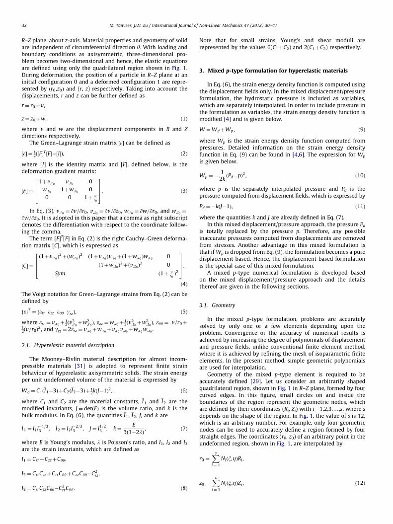
Let us consider a deformation dependent pressure load q,positive in compression, acting perpendicular to the infinitesi-mally small length ds, shown in Fig. 2, at Z¼ þ1. The length ds

and its outward unit normal vector n, shown in Fig. 2, can beexpressed as

ds¼ 9np � s,x9 dx, ð27Þ

fng ¼np � s,x

9np � s,x9, ð28Þ

where np is the outward unit normal vector to R–Z plane asshown in Fig. 2 and s,x ¼ @s=@x is the tangent vector to ds.

The deformation dependent load can now be defined as

fFZg ¼�2pq

ZS

rfHgTfng dS: ð29Þ

Using Eqs. (16), (27), and (28), the deformation dependent load isexpressed by

fF gZ ¼�2pq

Z þ1

�1r½H�Tfng dx, ð30Þ

where fngT ¼ af�Z,x r,xg with a¼ þ1 at Z¼ þ1 and a¼�1 atZ¼�1 and r is given by Eq. (14).

Eq. (30) is linearized with respect to nodal degrees of freedom,which is achieved by the Taylor series expansion with higherorder terms neglected using the concept of directional derivative[33–35] and is given by

fF ðuþDuÞgZ � fF ðuÞgZþDfF ðuÞgZfDug, ð31Þ

where the directional derivative is

DfF ðuÞgZfDug ¼d

de

��e ¼ 0

fF ðuþeDuÞgZ: ð32Þ

∧

Fig. 2. Normal (n) and tangent ð@s=@xÞ to length ds in an arbitrary shaped

quadrilateral region.

By substituting Eq. (30) in Eq. (32), following is obtained:

DfF ðuÞgZfDug ¼�2pq

Z þ1

�1½H�T

d

de

��e ¼ 0

ðrþeDvÞa�ðz,xþeDw,xÞ

r,xþeDv,x

( ) !dx:

ð33Þ

Finally, Eq. (31) can be expressed as

fF ðuþDuÞgZ � fF ðuÞgZþ½Kf �ZfDug, ð34Þ

where ½Kf �Z ¼�2pqR þ1�1 ½Bf �Z dx is asymmetric tangent load

matrix. Here, in the expression for ½Kf �Z, the matrix ½Bf �Z is definedin Appendix A.

5. Solution procedure

The equations of motion can be expressed using the linearizeddeformation dependent load, Eq. (34), in Eq. (25), as

½M�f €ugþð½Kuu��½Kf �ÞfDugþ½Kup�fDPg ¼ fF g�fFug, ð35Þ

½Kpu�fDugþ½Kpp�fDPg ¼�fFpg: ð36Þ

On the right hand side of Eq. (34), the first term becomes theexternally applied load vector and the second term contributes tothe stiffness matrix [Kuu] in Eq. (35).

If the solution involves more than one element, the equationsof motion, Eqs. (35) and (36), need to be assembled. After thevectors and matrices are assembled, the incremental pressures,fDpg, can be condensed out and the equations can be solved forincremental displacements, fDug, only. Using Eq. (36), the incre-mental pressure vector is expressed by

fDPg ¼�½Kpp��1ðfFpgþ½Kpu�fDugÞ: ð37Þ

By substituting Eq. (37) into Eq. (35), equations of motion interms of incremental displacements are defined as

½M�f €ugþ½K �fDug ¼ fF g�fF g, ð38Þ

where

½K � ¼ ½Kuu��½Kf ��½Kup�½Kpp��1½Kpu�, ð39Þ

fF g ¼ fFug�½Kup�½Kpp��1fFpg: ð40Þ

The vectors and matrices in Eq. (38) are integrated numericallyby the Gaussian quadrature method, where the number ofintegration points to obtain the accurate results depends on thedegrees of polynomials used in the solution. The equations ofmotion, expressed by Eq. (38), are solved by the Newmark’smethod, where the equations are set at time tþDt and at eachtime step Dt, equilibrium iterations are carried out by the New-ton–Raphson iterative technique. The equilibrium equations attime tþDt are expressed as

½M�f €ugitþDtþ½K �i�1t fDugi ¼ fF gtþDt�fF g

i�1tþDt , ð41Þ

where i¼ iteration number and

fugitþDt ¼ fugi�1tþDtþfDugi: ð42Þ

Matrices [M] and [Kpp] are constant and calculated before thetime integration. The same matrices are repeatedly used in thesolution procedure without any changes. All other vectors andmatrices are functions of displacements and are updated duringthe equilibrium iterations.

In the Newmark’s method [4], the values for acceleration andvelocities at time tþDt are

f €ugitþDt ¼ a0ðfugitþDt�fugtÞ�a2f _ugt�a3f €ugt , ð43Þ

f _ugtþDt ¼ f _ugt�a6f €ugtþa7f €ugtþDt , ð44Þ


where a0 ¼ 1=aðDtÞ2, a2 ¼ 1=aDt, a3 ¼ 1=2a�1, a6 ¼Dtð1�dÞ,and a7 ¼ dDt are the integration constants and a and d are theparameters, chosen to be 1

4 and 12 respectively, representing the

constant-average-acceleration method.Note that the pressures are also updated during the equili-

brium iterations, which are

fPgitþDt ¼ fPgi�1tþDtþfDPgi, ð45Þ

where fDPgi is obtained from Eq. (37) with fFpg and ½Kpu�

calculated at i�1.

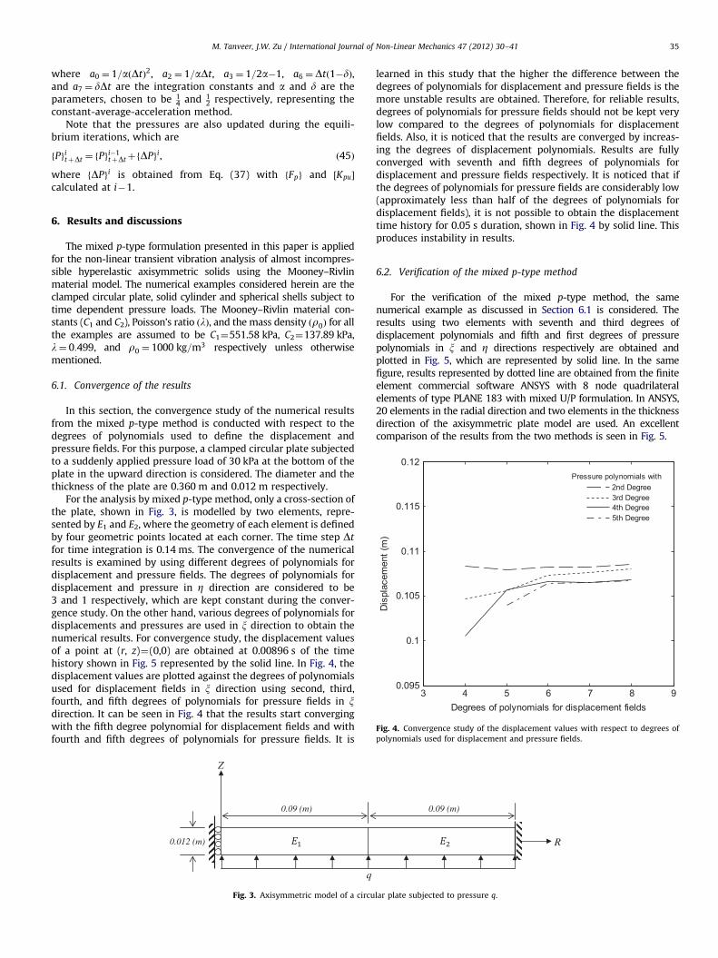
3 4 5 6 7 8 90.095

0.1

0.105

0.11

0.115

0.12

Degrees of polynomials for displacement fields

Dis

plac

emen

t (m

)

Pressure polynomials with2nd Degree3rd Degree4th Degree5th Degree

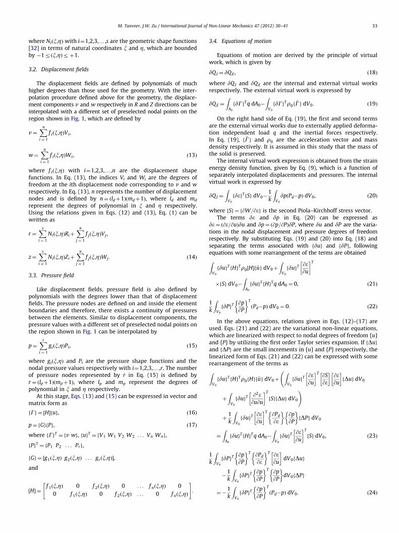
Fig. 4. Convergence study of the displacement values with respect to degrees of

polynomials used for displacement and pressure fields.

6. Results and discussions

The mixed p-type formulation presented in this paper is appliedfor the non-linear transient vibration analysis of almost incompres-sible hyperelastic axisymmetric solids using the Mooney–Rivlinmaterial model. The numerical examples considered herein are theclamped circular plate, solid cylinder and spherical shells subject totime dependent pressure loads. The Mooney–Rivlin material con-stants (C1 and C2), Poisson’s ratio ðlÞ, and the mass density ðr0Þ for allthe examples are assumed to be C1¼551.58 kPa, C2¼137.89 kPa,l¼ 0:499, and r0 ¼ 1000 kg=m3 respectively unless otherwisementioned.

6.1. Convergence of the results

In this section, the convergence study of the numerical resultsfrom the mixed p-type method is conducted with respect to thedegrees of polynomials used to define the displacement andpressure fields. For this purpose, a clamped circular plate subjectedto a suddenly applied pressure load of 30 kPa at the bottom of theplate in the upward direction is considered. The diameter and thethickness of the plate are 0.360 m and 0.012 m respectively.

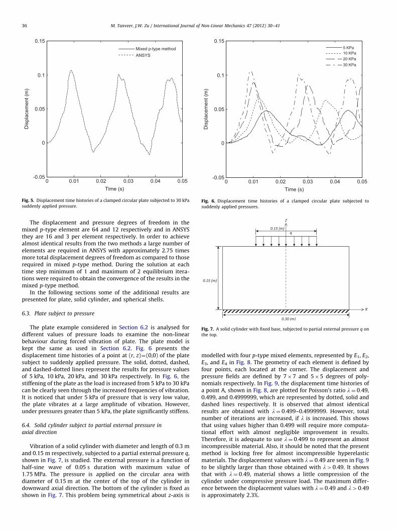
For the analysis by mixed p-type method, only a cross-section ofthe plate, shown in Fig. 3, is modelled by two elements, repre-sented by E1 and E2, where the geometry of each element is definedby four geometric points located at each corner. The time step Dt

for time integration is 0.14 ms. The convergence of the numericalresults is examined by using different degrees of polynomials fordisplacement and pressure fields. The degrees of polynomials fordisplacement and pressure in Z direction are considered to be3 and 1 respectively, which are kept constant during the conver-gence study. On the other hand, various degrees of polynomials fordisplacements and pressures are used in x direction to obtain thenumerical results. For convergence study, the displacement valuesof a point at (r, z)¼(0,0) are obtained at 0.00896 s of the timehistory shown in Fig. 5 represented by the solid line. In Fig. 4, thedisplacement values are plotted against the degrees of polynomialsused for displacement fields in x direction using second, third,fourth, and fifth degrees of polynomials for pressure fields in xdirection. It can be seen in Fig. 4 that the results start convergingwith the fifth degree polynomial for displacement fields and withfourth and fifth degrees of polynomials for pressure fields. It is

q

0.012 (m)

Z

)m(90.0

Fig. 3. Axisymmetric model of a circu

learned in this study that the higher the difference between thedegrees of polynomials for displacement and pressure fields is themore unstable results are obtained. Therefore, for reliable results,degrees of polynomials for pressure fields should not be kept verylow compared to the degrees of polynomials for displacementfields. Also, it is noticed that the results are converged by increas-ing the degrees of displacement polynomials. Results are fullyconverged with seventh and fifth degrees of polynomials fordisplacement and pressure fields respectively. It is noticed that ifthe degrees of polynomials for pressure fields are considerably low(approximately less than half of the degrees of polynomials fordisplacement fields), it is not possible to obtain the displacementtime history for 0.05 s duration, shown in Fig. 4 by solid line. Thisproduces instability in results.

6.2. Verification of the mixed p-type method

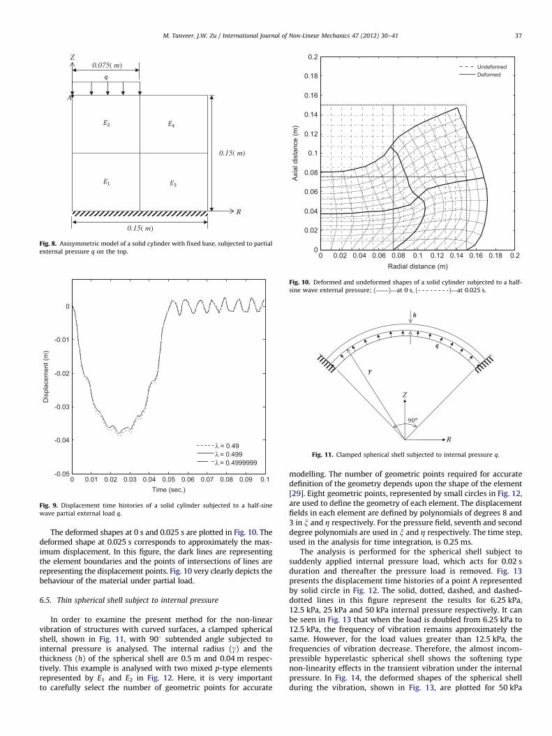
For the verification of the mixed p-type method, the samenumerical example as discussed in Section 6.1 is considered. Theresults using two elements with seventh and third degrees ofdisplacement polynomials and fifth and first degrees of pressurepolynomials in x and Z directions respectively are obtained andplotted in Fig. 5, which are represented by solid line. In the samefigure, results represented by dotted line are obtained from the finiteelement commercial software ANSYS with 8 node quadrilateralelements of type PLANE 183 with mixed U/P formulation. In ANSYS,20 elements in the radial direction and two elements in the thicknessdirection of the axisymmetric plate model are used. An excellentcomparison of the results from the two methods is seen in Fig. 5.

R

)m(90.0

lar plate subjected to pressure q.

0 0.01 0.02 0.03 0.04 0.05-0.05

0

0.05

0.1

0.15

Time (s)

Dis

plac

emen

t (m

)

Mixed p-type methodANSYS

Fig. 5. Displacement time histories of a clamped circular plate subjected to 30 kPa

suddenly applied pressure.

0 0.01 0.02 0.03 0.04 0.05-0.05

0

0.05

0.1

0.15

Time (s)

Dis

plac

emen

t (m

)

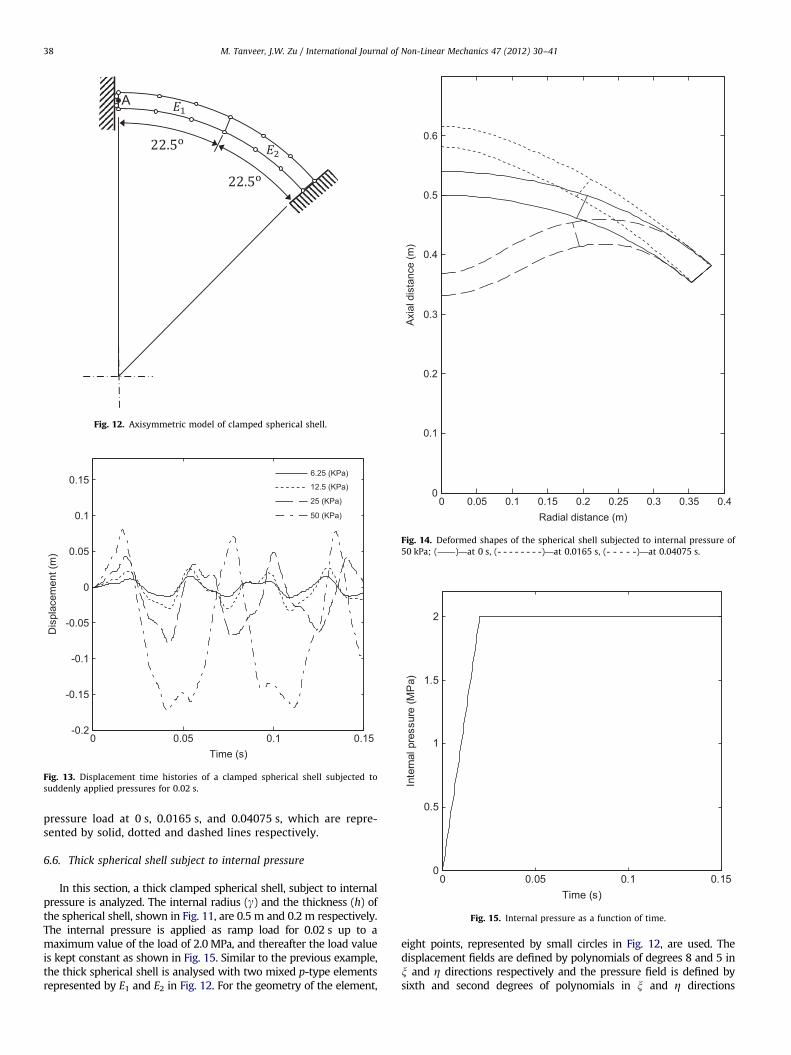
5 KPa10 KPa20 KPa30 KPa

Fig. 6. Displacement time histories of a clamped circular plate subjected to

suddenly applied pressures.

Fig. 7. A solid cylinder with fixed base, subjected to partial external pressure q on

the top.


The displacement and pressure degrees of freedom in themixed p-type element are 64 and 12 respectively and in ANSYSthey are 16 and 3 per element respectively. In order to achievealmost identical results from the two methods a large number ofelements are required in ANSYS with approximately 2.75 timesmore total displacement degrees of freedom as compared to thoserequired in mixed p-type method. During the solution at eachtime step minimum of 1 and maximum of 2 equilibrium itera-tions were required to obtain the convergence of the results in themixed p-type method.

In the following sections some of the additional results arepresented for plate, solid cylinder, and spherical shells.

6.3. Plate subject to pressure

The plate example considered in Section 6.2 is analysed fordifferent values of pressure loads to examine the non-linearbehaviour during forced vibration of plate. The plate model iskept the same as used in Section 6.2. Fig. 6 presents thedisplacement time histories of a point at (r, z)¼(0,0) of the platesubject to suddenly applied pressure. The solid, dotted, dashed,and dashed-dotted lines represent the results for pressure valuesof 5 kPa, 10 kPa, 20 kPa, and 30 kPa respectively. In Fig. 6, thestiffening of the plate as the load is increased from 5 kPa to 30 kPacan be clearly seen through the increased frequencies of vibration.It is noticed that under 5 kPa of pressure that is very low value,the plate vibrates at a large amplitude of vibration. However,under pressures greater than 5 kPa, the plate significantly stiffens.

6.4. Solid cylinder subject to partial external pressure in

axial direction

Vibration of a solid cylinder with diameter and length of 0.3 mand 0.15 m respectively, subjected to a partial external pressure q,shown in Fig. 7, is studied. The external pressure is a function ofhalf-sine wave of 0.05 s duration with maximum value of1.75 MPa. The pressure is applied on the circular area withdiameter of 0.15 m at the center of the top of the cylinder indownward axial direction. The bottom of the cylinder is fixed asshown in Fig. 7. This problem being symmetrical about z-axis is

modelled with four p-type mixed elements, represented by E1, E2,E3, and E4 in Fig. 8. The geometry of each element is defined byfour points, each located at the corner. The displacement andpressure fields are defined by 7�7 and 5�5 degrees of poly-nomials respectively. In Fig. 9, the displacement time histories ofa point A, shown in Fig. 8, are plotted for Poisson’s ratio l¼ 0:49,0.499, and 0.4999999, which are represented by dotted, solid anddashed lines respectively. It is observed that almost identicalresults are obtained with l¼ 0:499–0.4999999. However, totalnumber of iterations are increased, if l is increased. This showsthat using values higher than 0.499 will require more computa-tional effort with almost negligible improvement in results.Therefore, it is adequate to use l¼ 0:499 to represent an almostincompressible material. Also, it should be noted that the presentmethod is locking free for almost incompressible hyperelasticmaterials. The displacement values with l¼ 0:49 are seen in Fig. 9to be slightly larger than those obtained with l40:49. It showsthat with l¼ 0:49, material shows a little compression of thecylinder under compressive pressure load. The maximum differ-ence between the displacement values with l¼ 0:49 and l40:49is approximately 2.3%.

0 0.01 0.02 0.03 0.04 0.05 0.06 0.07 0.08 0.09 0.1-0.05

-0.04

-0.03

-0.02

-0.01

0

Time (sec.)

Dis

plac

emen

t (m

)

= 0.49 = 0.499 = 0.4999999

Fig. 9. Displacement time histories of a solid cylinder subjected to a half-sine

wave partial external load q.

0 0.02 0.04 0.06 0.08 0.1 0.12 0.14 0.16 0.18 0.20

0.02

0.04

0.06

0.08

0.1

0.12

0.14

0.16

0.18

0.2

Radial distance (m)

Axi

al d

ista

nce

(m)

UndeformedDeformed

Fig. 10. Deformed and undeformed shapes of a solid cylinder subjected to a half-

sine wave external pressure; (——)—at 0 s, (- - - - - - - -)—at 0.025 s.

Z

h

R

q

Fig. 11. Clamped spherical shell subjected to internal pressure q.

A

R

Z

0.15( m)

0.075( m)

0.15( m)

Fig. 8. Axisymmetric model of a solid cylinder with fixed base, subjected to partial

external pressure q on the top.


The deformed shapes at 0 s and 0.025 s are plotted in Fig. 10. Thedeformed shape at 0.025 s corresponds to approximately the max-imum displacement. In this figure, the dark lines are representingthe element boundaries and the points of intersections of lines arerepresenting the displacement points. Fig. 10 very clearly depicts thebehaviour of the material under partial load.

6.5. Thin spherical shell subject to internal pressure

In order to examine the present method for the non-linearvibration of structures with curved surfaces, a clamped sphericalshell, shown in Fig. 11, with 901 subtended angle subjected tointernal pressure is analysed. The internal radius (g) and thethickness (h) of the spherical shell are 0.5 m and 0.04 m respec-tively. This example is analysed with two mixed p-type elementsrepresented by E1 and E2 in Fig. 12. Here, it is very importantto carefully select the number of geometric points for accurate

modelling. The number of geometric points required for accuratedefinition of the geometry depends upon the shape of the element[29]. Eight geometric points, represented by small circles in Fig. 12,are used to define the geometry of each element. The displacementfields in each element are defined by polynomials of degrees 8 and3 in x and Z respectively. For the pressure field, seventh and seconddegree polynomials are used in x and Z respectively. The time step,used in the analysis for time integration, is 0.25 ms.

The analysis is performed for the spherical shell subject tosuddenly applied internal pressure load, which acts for 0.02 sduration and thereafter the pressure load is removed. Fig. 13presents the displacement time histories of a point A representedby solid circle in Fig. 12. The solid, dotted, dashed, and dashed-dotted lines in this figure represent the results for 6.25 kPa,12.5 kPa, 25 kPa and 50 kPa internal pressure respectively. It canbe seen in Fig. 13 that when the load is doubled from 6.25 kPa to12.5 kPa, the frequency of vibration remains approximately thesame. However, for the load values greater than 12.5 kPa, thefrequencies of vibration decrease. Therefore, the almost incom-pressible hyperelastic spherical shell shows the softening typenon-linearity effects in the transient vibration under the internalpressure. In Fig. 14, the deformed shapes of the spherical shellduring the vibration, shown in Fig. 13, are plotted for 50 kPa

0 0.05 0.1 0.15-0.2

-0.15

-0.1

-0.05

0

0.05

0.1

0.15

Time (s)

Dis

plac

emen

t (m

)

6.25 (KPa)

12.5 (KPa)

25 (KPa)

50 (KPa)

Fig. 13. Displacement time histories of a clamped spherical shell subjected to

suddenly applied pressures for 0.02 s.

0 0.05 0.1 0.15 0.2 0.25 0.3 0.35 0.40

0.1

0.2

0.3

0.4

0.5

0.6

Radial distance (m)

Axi

al d

ista

nce

(m)

Fig. 14. Deformed shapes of the spherical shell subjected to internal pressure of

50 kPa; (——)—at 0 s, (- - - - - - - -)—at 0.0165 s, (- - - - -)—at 0.04075 s.

0 0.05 0.1 0.150

0.5

1

1.5

2

Time (s)

Inte

rnal

pre

ssur

e (M

Pa)

Fig. 15. Internal pressure as a function of time.

A

Fig. 12. Axisymmetric model of clamped spherical shell.


pressure load at 0 s, 0.0165 s, and 0.04075 s, which are repre-sented by solid, dotted and dashed lines respectively.

6.6. Thick spherical shell subject to internal pressure

In this section, a thick clamped spherical shell, subject to internalpressure is analyzed. The internal radius (g) and the thickness (h) ofthe spherical shell, shown in Fig. 11, are 0.5 m and 0.2 m respectively.The internal pressure is applied as ramp load for 0.02 s up to amaximum value of the load of 2.0 MPa, and thereafter the load valueis kept constant as shown in Fig. 15. Similar to the previous example,the thick spherical shell is analysed with two mixed p-type elementsrepresented by E1 and E2 in Fig. 12. For the geometry of the element,

eight points, represented by small circles in Fig. 12, are used. Thedisplacement fields are defined by polynomials of degrees 8 and 5 inx and Z directions respectively and the pressure field is defined bysixth and second degrees of polynomials in x and Z directions

0 0.05 0.1 0.150

0.2

0.4

0.6

0.8

1

1.2

Time (s)

Dis

plac

emen

t (m

)

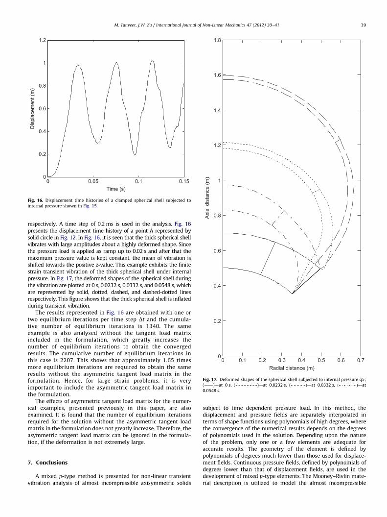
Fig. 16. Displacement time histories of a clamped spherical shell subjected to

internal pressure shown in Fig. 15.

0 0.1 0.2 0.3 0.4 0.5 0.6 0.70

0.2

0.4

0.6

0.8

1

1.2

1.4

1.6

1.8

Radial distance (m)

Axi

al d

ista

nce

(m)

Fig. 17. Deformed shapes of the spherical shell subjected to internal pressure q5;

(——)—at 0 s, (- - - - - - - -)—at 0.0232 s, (- - - - -)—at 0.0332 s, ð- � - � - � -�Þ—at

0.0548 s.


respectively. A time step of 0.2 ms is used in the analysis. Fig. 16presents the displacement time history of a point A represented bysolid circle in Fig. 12. In Fig. 16, it is seen that the thick spherical shellvibrates with large amplitudes about a highly deformed shape. Sincethe pressure load is applied as ramp up to 0.02 s and after that themaximum pressure value is kept constant, the mean of vibration isshifted towards the positive z-value. This example exhibits the finitestrain transient vibration of the thick spherical shell under internalpressure. In Fig. 17, the deformed shapes of the spherical shell duringthe vibration are plotted at 0 s, 0.0232 s, 0.0332 s, and 0.0548 s, whichare represented by solid, dotted, dashed, and dashed-dotted linesrespectively. This figure shows that the thick spherical shell is inflatedduring transient vibration.

The results represented in Fig. 16 are obtained with one ortwo equilibrium iterations per time step Dt and the cumula-tive number of equilibrium iterations is 1340. The sameexample is also analysed without the tangent load matrixincluded in the formulation, which greatly increases thenumber of equilibrium iterations to obtain the convergedresults. The cumulative number of equilibrium iterations inthis case is 2207. This shows that approximately 1.65 timesmore equilibrium iterations are required to obtain the sameresults without the asymmetric tangent load matrix in theformulation. Hence, for large strain problems, it is veryimportant to include the asymmetric tangent load matrix inthe formulation.

The effects of asymmetric tangent load matrix for the numer-ical examples, presented previously in this paper, are alsoexamined. It is found that the number of equilibrium iterationsrequired for the solution without the asymmetric tangent loadmatrix in the formulation does not greatly increase. Therefore, theasymmetric tangent load matrix can be ignored in the formula-tion, if the deformation is not extremely large.

7. Conclusions

A mixed p-type method is presented for non-linear transientvibration analysis of almost incompressible axisymmetric solids

subject to time dependent pressure load. In this method, thedisplacement and pressure fields are separately interpolated interms of shape functions using polynomials of high degrees, wherethe convergence of the numerical results depends on the degreesof polynomials used in the solution. Depending upon the natureof the problem, only one or a few elements are adequate foraccurate results. The geometry of the element is defined bypolynomials of degrees much lower than those used for displace-ment fields. Continuous pressure fields, defined by polynomials ofdegrees lower than that of displacement fields, are used in thedevelopment of mixed p-type elements. The Mooney–Rivlin mate-rial description is utilized to model the almost incompressible


hyperelastic material. The total Lagrangian formulation is adoptedfor axisymmetric solids of revolution. The equations of motion arederived using the principle of virtual work and solved by New-marks’s method in conjunction with the Newton–Raphson iterativetechnique. The asymmetric tangent load matrix that results inlinearization of deformation dependent load is also included in theformulation.

Circular plates, solid cylinder and spherical shells subject topressure load are analysed by the mixed p-type method. In orderto examine the numerical stability of the method, a convergencestudy of the results is presented with respect to the degrees ofpolynomials used for displacement and pressure fields. Themethod is verified by successfully comparing the results withthose obtained from the finite element method using the com-mercial software ANSYS. Several results are presented for thetransient vibration under different time dependent pressure loadsand the highly non-linear behaviour is examined and discussed.In plates, the frequencies of transient vibrations under suddenlyapplied pressure loads are seen to be increasing at large ampli-tudes. However, for thin spherical shell under suddenly appliedinternal pressures for limited duration, the frequencies of vibra-tion reduce with increasing amplitudes of vibration. The thickspherical shell under internal pressure of ramp type is found toundergo large strains and be inflated during vibration.

The present method is very efficient, which yields accurateresults at finite strains with high convergence rate. The conver-gence of the results in this method does not require a largenumber of elements or the total degrees of freedom as it isrequired in conventional finite element method. However, it isnoticed that the instability in results exists, if the degrees ofpressure polynomials are considerably lower than the degrees ofdisplacement polynomial. The inclusion of asymmetric tangentload matrix in the formulation greatly reduces the number ofequilibrium iterations to get the convergence of results for largestrain vibration problems.

Acknowledgments

Natural Sciences and Engineering Research Council of Canada(NSERC) is greatly acknowledged for the financial support for thisresearch work. Shared Hierarchical Academic Research Comput-ing Network (SHARCNET) Canada is also acknowledged for pro-viding high performance computing facilities.

Appendix A

Matrices and vectors in Eqs. (25) and (26) are defined below

½M� ¼ 2pZ þ1

�1

Z þ1

�1r0½H�

T ½H�r09J09 dx dZ, ðA:1Þ

½Kuu� ¼ ½Kuu�1þ½Kuu�2, ðA:2Þ

½Kuu�1 ¼ 2pZ þ1

�1

Z þ1

�1½BL�

T ½D�½BL�r09J09 dx dZ, ðA:3Þ

½Kuu�2 ¼ 2pZ þ1

�1

Z þ1

�1½BNL�

T ½S�½BNL�r09J09 dx dZ, ðA:4Þ

½Kup� ¼ 2pZ þ1

�1

Z þ1

�1½BL�

TfBpdgfGgr09J09 dx dZ, ðA:5Þ

½Kpu� ¼ ½Kup�T , ðA:6Þ

½Kpp� ¼ �2pZ þ1

�1

Z þ1

�1fGgT

1

kfGgr09J09 dx dZ, ðA:7Þ

fFug ¼ 2pZ þ1

�1

Z þ1

�1½BL�

TfSgr09J09 dx dZ, ðA:8Þ

fFpg ¼ 2pZ þ1

�1

Z þ1

�1fGgT ðPd�pÞr09J09 dx dZ, ðA:9Þ

where 9J09 is the determinant of Jacobian transformation betweenthe local coordinates ðx,ZÞ and the global coordinate (r0, z0) andthe matrices [BL], [BNL], [D], ½S� and vectors fBpd

g, {S} are defined asfollows:

½BL� ¼ ½dL�½H�, ðA:10Þ

½BNL� ¼ ½dNL�½H�, ðA:11Þ

where

½dL�T ¼

ð1þv,r0Þ @@r0

ðv,z0Þ @@z0

ð1þ vr0Þ 1

r0ð1þv,r0

Þ @@z0þðv,z0

Þ @@r0

ðw,r0Þ @@r0

ð1þw,z0Þ @@z0

0 ðw,r0Þ @@z0þð1þw,z0

Þ @@r0

24

35

and

½dNL�T ¼

@@r0

0 1r0

@@r0

0

0 @@z0

0 0 @@z0

24

35:

Eq. (2), in terms of the right Cauchy–Green deformation [C], canbe expressed as ½e� ¼ 1

2ð½C��½I�Þ and using this relation the followingoperator is introduced:

@ð Þ

@eij¼ 2

@ð Þ

@Cij: ðA:12Þ

In all the expressions defined below, the relation given byEq. (A.12) is used.

The vector fBpdg in Eq. (A.5) is expressed as

fBpdgT ¼

@Pd

@err

@Pd

@ezz

@Pd

@eyy@Pd

@grz

� �, ðA:13Þ

which can be further defined as

fBpdgT ¼ �I�1=2

3

@I3

@Crr�I�1=2

3

@I3

@Czz�I�1=2

3

@I3

@Cyy�

1

2I�1=23

@I3

@Crz

� �:

ðA:14Þ

The non-zero values in the second Piola–Kirchhoff stressmatrix ½S�5�5 in Eq. (A.4) are S11 ¼ S44 ¼ Srr , S12 ¼ S21 ¼ S45 ¼

S54 ¼ Srz, S22 ¼ S55 ¼ Szz, and S33 ¼ Syy.The matrix [D] in Eq. (A.3) is defined as

½D� ¼

2 @Srr@Crr

2 @Srr@Czz

2 @Srr@Cyy

@Srr@Crz

2 @Szz

@Czz2 @Szz

@Cyy

@Szz

@Crz

2 @Syy@Cyy

@Syy@Crz

Sym: @Srz

@Crz

26666664

37777775

, ðA:15Þ

where

@Sij

@Ckl¼ a C1

@

@Ckl

@J1

@Cij

� �þC2

@

@Ckl

@J2

@Cij

� ��þk

@J3

@Cij

@J3

@CklþðJ3�1Þ

@

@Ckl

�

�@J3

@Cij

� ��

1

k

@Pd

@Cij

@Pd

@Ckl�

1

kðPd�pÞ

@

@Ckl

@Pd

@Cij

� ��ðA:16Þ

with a¼1 if ia j and a¼2 if i¼ j.Some of the terms used in Eq. (A.16) are given below

@J1

@Cij¼ I�1=3

3

@I1

@Cij�

1

3I1I�4=3

3

@I3

@Cij,

@J2

@Cij¼ I�2=3

3

@I2

@Cij�

2

3I2I�5=3

3

@I3

@Cij,

@J3

@Cij¼

1

2I�1=33

@I3

@Cij,

@Pd

@Cij¼�

1

2kI�1=2

3

@I3

@Cij:


The second Piola–Kirchhoff stress vector {S} in Eq. (A.8) is defined as

fSgT ¼ fSrr Szz Syy Srzg, ðA:17Þ

where

Srr ¼ 2@Wd

@Crr�

1

kðPd�pÞ

@Pd

@Crr

� �, Szz ¼ 2

@Wd

@Czz�

1

kðPd�pÞ

@Pd

@Czz

� �,

Syy ¼ 2@Wd

@Cyy�

1

kðPd�pÞ

@Pd

@Cyy

� �,

and

Srz ¼@Wd

@Crz�

1

kðPd�pÞ

@Pd

@Crz:

The expanded form of the second Piola–Kirchhoff stress can beexpressed as

Sij ¼ a C1@J1

@CijþC2

@J2

@CijþkðJ3�1Þ

@J3

@Cij�

1

kðPd�pÞ

@Pd

@Cij

� �, ðA:18Þ

where a¼1 if ia j and a¼2 if i¼ j.The matrix ½Bf �Z in Eq. (34) is defined as

½Bf �Z ¼ a

b11f 1 d11f 1 b12f 1 d12f 1 . . . b1nf 1 d1nf 1

e11f 1 0 e12f 1 0 . . . e1nf 1 0

b21f 2 d21f 2 b22f 2 d22f 2 . . . b2nf 2 d2nf 2

e21f 2 0 e22f 2 0 . . . e2nf 2 0

^ ^ ^ ^ ^ ^ ^

^ ^ ^ ^ ^ ^ ^

bn1f n dn1f n bn2f n dn2f n . . . bnnf n dnnf n

en1f n 0 en2f n 0 . . . ennf n 0

2666666666666664

3777777777777775

,

ðA:19Þ

where bij ¼�z,xðx,ZÞf jðx,ZÞ, dij ¼�rðx,ZÞf j,xðx,ZÞ, and eij ¼ r,xðx,ZÞf jðx,ZÞþrðx,ZÞf j,xj

ðx,ZÞ with i,j¼ 1;2,3, . . . ,n.

References

[1] M. Kaliske, H. Robert, On the finite element implementation of rubber-likematerials at finite strains, Engineering Computations 14 (2) (1997) 216–232.

[2] G. Saccomandi, R.W. Ogden, Mechanics and Thermomechanics of RubberlikeSolids, Springer, New York, 2004.

[3] A.P.S. Selvadurrai, Deflections of rubber membrane, Journal of the Mechanicsand Physics of Solids 54 (2006) 1093–1119.

[4] K.-J. Bathe, Finite Element Procedures, Prentice-Hall, New Jersey, 1996.[5] M.S. Gadala, Numerical solutions of nonlinear problems of continua—II.

Survey of incompressibility constraints and software aspects, Computers &Structures 22 (5) (1986) 841–855.

[6] T. Sussman, K.-J. Bathe, A finite element formulation for nonlinear incom-pressible elastic and inelastic analysis, Computers & Structures 26 (1/2)(1987) 357–409.

[7] L. Mackerle, Rubber and rubber-like materials, finite element analyses andsimulations: a bibliography (1976–1997), Modeling and Simulation inMaterial Science and Engineering 6 (1998) 171–198.

[8] L. Mackerle, Rubber and rubber-like materials, finite element analyses andsimulations, an addendum: a bibliography (1997–2003), Modeling andSimulation in Material Science and Engineering 12 (2004) 1031–1053.

[9] L.R. Herrmann, Elasticity equations for incompressible and nearly incompres-sible materials by a variational theorem, AIAA Journal 3 (1965) 1896–1900.

[10] R.L. Taylor, K.S. Pister, L.R. Herrmann, On a variational theorem for incom-pressible and nearly-incompressible orthotropic elasticity, InternationalJournal of Solids and Structures 4 (1968) 875–883.

[11] S.W. Key, A variational principle for incompressible and nearly-incompres-sible anisotropic elasticity, International Journal of Solids and Structures5 (1969) 951–964.

[12] J.T. Oden, J.E. Key, Numerical analysis of finite axisymmetric deformation ofincompressible elastic solids of revolution, International Journal of Solids andStructures 6 (1970) 497–518.

[13] T. Scharnhorst, T.H.H. Pian, Finite element analysis of rubber-like materialsby a mixed model, International Journal for Numerical Methods in Engineer-ing 12 (1978) 665–676.

[14] H. Murakawa, S.N. Atluri, Finite elasticity solutions using hybrid finiteelements based on a complementary energy principle, Journal of AppliedMechanics 45 (1978) 539–547.

[15] R.C. Batra, Finite plane strain deformations of rubberlike materials, Interna-tional Journal for Numerical Methods in Engineering 15 (1980) 147–160.

[16] R. Srinivasan, R. Perucchio, Finite element analysis of anisotropic non-linearincompressible elastic solids by a mixed model, International Journal forNumerical Methods in Engineering 37 (1994) 3075–3092.

[17] P.A. Kakavas, G.I. Giannopoulos, N.K. Anifantis, Mixed finite element analysisof elastomeric butt-joints, ASME Journal of Engineering Materials andTechnology 129 (2007) 11–18.

[18] D.S. Malkus, T.J.R. Hughes, Mixed finite element methods-reduced andselective integration techniques; a unification of concepts, Computer Meth-ods in Applied Mechanics and Engineering 15 (1978) 63–81.

[19] K.-D. Papoulia, Mixed and selective reduced integration procedures in largestrain hyperelastic analysis of nearly incompressible solids, ComputationalMechanics 23 (1999) 63–74.

[20] F. Brezzi, On the existence, uniqueness and approximation of saddle-pointproblems arising from Lagrangian multipliers, RAIRO 8 (1974) 129–151.

[21] I. Babuska, The finite element method with Lagrangian multipliers, Numer-ische Mathematik 20 (1973) 179–192.

[22] I. Babuska, The finite element method with penalty, Mathematics of Compu-tation 27 (1973) 221–228.

[23] T.J.R. Hughes, The Finite Element Method: Linear Static and Dynamic FiniteElement Analysis, Dover Publications, Inc., New York, 2000.

[24] O.C. Zienkiewicz, S. Qu, R.L. Taylor, S. Nakazawa, The patch test for mixedformulations, International Journal for Numerical Methods in Engineering23 (1986) 1873–1883.

[25] A. Duster, S. Hartmann, E. Rank, p-FEM applied to finite isotropic hyperelasticbodies, Computer Methods in Applied Mechanics and Engineering 192 (2003)5147–5166.

[26] Y. Basar, U. Hanskotter, Ch. Schwab, A general high-order finite elementformulation for shells at large strains and finite rotations, InternationalJournal for Numerical Methods in Engineering 57 (2003) 2147–2175.

[27] C. Wielgosz, G. Marckmann, Dynamic analysis of nonlinear elastic materials,Computational Materials Science 7 (1996) 1–4.

[28] K. Miller, G. Joldes, D. Lance, A. Wittek, Total Lagrangian explicit finiteelement algorithm for computing soft tissue deformation, Communicationsin Numerical Methods in Engineering 23 (2007) 121–134.

[29] T. Muhammad, A.V. Singh, A p-type solution for the bending of rectangular,circular, elliptic, and skew plates, International Journal of Solids andStructures 41 (2004) 3977–3997.

[30] ANSYS Release 12, ANSYS Inc., Canonsburg, PA 15317.[31] M.A. Crisfield, Non-linear Finite Element Analysis of Solids and Structures,

John Wiley & Sons, West Sussex, 1991.[32] W. Weaver, P.R. Johnston, Finite Elements for Structural Analysis, Prentice-

Hall, New Jersey, 1984.[33] J. Bonet, R.D. Wood, Nonlinear Continuum Mechanics for Finite Element

Analysis, Cambridge University Press, Cambridge, 1997.[34] J.C. Simo, R.L. Taylor, P. Wriggers, A note on finite-element implementation of

pressure boundary loading, Communications in Applied Numerical Methods7 (1991) 513–525.

[35] Z. Yosibash, S. Hartmann, U. Heisserer, A. Duster, E. Rank, M. Szanto,Axisymmetric pressure boundary loading for finite deformation analysisusing p-FEM, Computer Methods in Applied Mechanics and Engineering196 (2007) 1261–1277.

Documents

Non-linear vibration of hyperelastic axisymmetric solids by a mixed p-type method