NON LINEAR SYSTEMS: ANALYSYS AND CONTROL - unibo.it · AC&ST C. Melchiorri (DEI) Automatic Control & System Theory 2 Non linear systems Analysis and design methods based on the assumption

AC&ST

C. Melchiorri (DEI) Automatic Control & System Theory 1

AUTOMATIC CONTROL AND SYSTEM THEORY

NON LINEAR SYSTEMS: ANALYSYS AND CONTROL

Claudio Melchiorri

Dipartimento di Ingegneria dell’Energia Elettrica e dell’Informazione (DEI) Università di Bologna

Email: [email protected]

AC&ST


Non linear systems

Analysis and design methods based on the assumption of linear and time-invariant systems are very common and allow to use efficient and relatively simple tools. On the other hand, the linearity assumption is justified only if the considered signals and variables of the system vary in relatively small ranges. As a matter of fact, all physical systems are non linear, and behave approximately as linear only for “small signals”. However, there are systems that do not show a linear behavior even for “small signals”. Note that a non linear behavior does not necessarily mean something to be avoided: there are systems in which non linearities are introduced on purpose in order to obtain specific behaviors.

G(S)

(x(t) = Ax(t) +Bu(t)

y(t) = Cx(t)

(x(t) = f(x, u, t)

y(t) = h(x, t)

AC&ST


Non linear systems

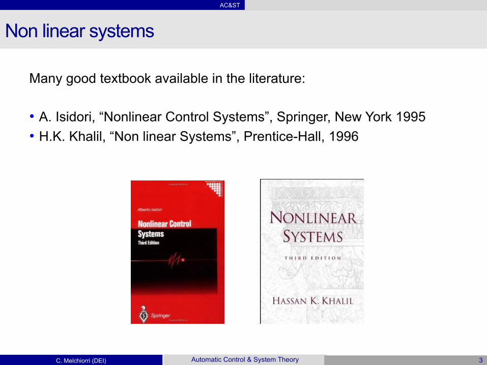
Many good textbook available in the literature: • A. Isidori, “Nonlinear Control Systems”, Springer, New York 1995 • H.K. Khalil, “Non linear Systems”, Prentice-Hall, 1996

AC&ST


Non linear systems

Problems with non linear systems: 1)  Analysis of the stability properties

a.  Linearization (first Lyapunov method) b.  Lyapunov (second Lyapunov method) c.  Phase-plane plot (equilibrium points, limit cycles) d.  Circle criterion e.  Popov criterion

2)  Design of control systems a.  Based on Lyapunov techniques b.  Feedback linearization c.  …

AC&ST


Circle Criterion – Popov Criterion

Goal: study the global asymptotic stability of a non linear system. The “Circle criterion” and the “Popov criterion” give two sufficient conditions for the GAS of feedback autonomous, non linear systems in which a non linear algebraic part and a linear (stable) dynamics can be identified: A scheme of this type is obtained from the more general scheme when r = cost.

-G(s) x y

G2(s) x y

H(s)

G1(s) r e c

- +

y = φ(x, t)

AC&ST


Circle Criterion

Sector condition A non linear memoryless function φ(x, t) is said to satisfy a sector condition if some constants α, β, a, b (with b > a, α < 0 < β,) exist such that

If this condition hold ∀ y ∈(-∞, +∞), the sector condition holds globally and φ(x, t) belongs to the sector [a, b]

ay2 y '(y, t) by2, 8t � 0, 8y 2 [↵,�]

x

y

a 1

b

y = φ(x, t)

AC&ST


Circle Criterion

The circle criterion may be considered as an extension of the Nyquist criterion for stability of SISO linear systems. THEOREM Consider a linear system subject to non-linear feedback, i.e. a non linear element φ(x, t) is present in the feedback loop. Assume that φ(x, t) satisfies globally a sector condition [a, b]. Then the closed loop system is globally asymptotically stable if one of the following three conditions is satisfied: 1)  If 0 < a < b, the Nyquist plot of G(j ω) does not penetrate the circle having

as diameter the segment [-1/a,-1/b] (the “critical circle” D(a, b)) located on the x-axis and it surrounds the circle D(a,b) counterclockwise m times, being m the number of unstable poles of G(s)

2)  If 0 = a < b, G(s) is stable and the Nyquist plot of G(j ω) is located on the right of the vertical line Re(s) = -1/b

3)  If a < 0 < b, G(s) is stable and the Nyquist plot of G(j ω) is within the circle D(a,b)

AC&ST


Circle Criterion

The circle criterion is very simple to be verified. It may be considered as an extension to the non linear case of the Nyquist criterion. The Nyquist criterion is obtained in case a = b = m (linear case): the point -1/m (limit case of the circle when a = b = m) must not be encircled by the Nyquist plot.

x

y

a 1

b

y = φ(x, t)

Im(G(j ω))

Re(G(j ω))

-1/b -1/a

AC&ST


Circle Criterion - Example

m = 1 m = 2 m = 3

m = 4 m = 5 G(s) =

10000

(s+ 10)4

AC&ST


Circle Criterion

A quite frequent case is when a = 0 (sector [0, b]) (e.g. saturation). In this case the circle degenerates to the half plane to the left of point -1/b.

x

y b

y = φ(x, t)

Im(G(j ω))

Re(G(j ω))

-1/b

AC&ST


Circle Criterion

Example 1. Study the GAS of the following system

G(s) =1

(s+ 2)(s+ 3)

0.1667

-0.021

AC&ST


Circle Criterion


G(s) =1

(s+ 2)(s+ 3)

Since G(s) is stable, it is possible to consider a < 0 and apply the third case of the Theorem. A circle D(a,b) encircling the Nyquist plot must be defined: several choices are possible! a) If the center of D(a, b) is placed in the origin, then the circle D(-r, r) must be defined, being r the maximum value of |G(j ω)|. From the plot, sup |G(j ω)| = 0.1667, then the system is GAS for all the nonlinearities in the sector [-1/0.1667, +1/0.1667] = [-6, 6].

0.1667

AC&ST


Circle Criterion


G(s) =1

(s+ 2)(s+ 3)

Since G(s) is stable, it is possible to consider a < 0 and apply the third case of the Theorem. A circle D(a,b) encircling the Nyquist plot must be defined: several choices are possible! b) If the center of D(a,b) is in (0.05, 0), then the maximum distance from this point to the Nyquist plot is 0.1167 (= r). The intersections of the circle with the real axis are -0.0667 (= -(0.1167 - 0.05)) and 0.1167. The system is GAS for all the nonlinearities in the sector [-1/0.1167, 1/0.0667] = [-6, +15].

0.1667 -0.0667

AC&ST


Circle Criterion


G(s) =1

(s+ 2)(s+ 3)

c) Let us assume a = 0 and apply the second case of the Theorem. The Nyquist plot is on the left of the vertical line Re(s) = -0.021. The system is GAS for all nonlinearities in the sector [0, 1/0.021] = [0, 47.619]. Note that this case gives the best estimation of b, but only nonlinearities in the first and third sectors are allowed!

0.1667

-0.021

AC&ST


Circle Criterion


G(s) =1

(s+ 2)(s+ 3)

Three different stability bounds have been identified. a)  [-6, 6] b)  [-6, +15] c)  [0, 47.619]

Notice that from the previous analysis we can conclude that the system is GAS for nonlinearities satisfying the sector condition [-6, 47.619].

a)

b)

c)

AC&ST


Circle Criterion


The system is non stable. Case 1) of the Theorem must then be considered (a > 0). The Nyquist plot must encircle counterclockwise the circle D(a,b) (once). Selecting the point c = [-0.15, 0] as center, the minimum distance between c and the Nyquist plot is 0.0873 (radius of the circle D(a,b)). The points on the real axis are: -1/b = -0.2373, -1/a = -0.0627. The system is GAS for all nonlinearities in the sector [1/0.2373, 1/0.0627] = [4.2141, 15.949].

G(s) =s+ 1

(s+ 2)2(s� 1)

-0.0627

-0.2373

AC&ST


Circle Criterion


The system is non stable: 2 poles with positive real part. Case 1) of the Theorem must be considered (a > 0): the Nyquist plot should encircle twice the circle D(a,b). Unfortunately, this is not possible! A sector for which the system is GAS does not exist!

G(s) =s

s2 � s+ 1p1,2 =

1

2±

p3

2j

AC&ST


Popov Criterion

The Popov criterion may be applied when: 1)  The non linear function φ(x) is defined in the sector [0, b] 2)  The non linear function satisfies φ(0) = 0 3)  The linear transfer function G(s) has deg(p(s)) < deg(q(s))

4)  The poles of G(s) are in the left hand side plane or on the imaginary axis 5)  The system is marginally stable in the singular case

G(s) =1

shp(s)

q(s)

AC&ST


Popov Criterion

THEOREM

The closed loop system is globally asymptotically stable if φ(x)∈[0, b], 0<b< ∞, and there exists a constant q such that the following equation is satisfied Graphical interpretation Let us define the Popov plot P as Then, the closed loop system is GAS if P lies to the right of the line through the point (–1/b + j 0) with a slope 1/q.

Re[G(j!)]� qj!Im[G(j!)] > �1

b, 8! 2 [�1,1]

P (j!) = {z = Re[G(j!)] + j!Im[G(j!)], ! > 0}

AC&ST


Popov Criterion

•  The Popov plot is not the same as the Nyquist plot (increased “difficulty”) •  The Popov criterion is less conservative than the Circle criterion: both are

sufficient conditions! (Popov may indicate GAS for systems for which the Circle criterion does not give indication)

•  Popov applies only to time-invariant nonlinearities φ(x), while the Circle criterion can be applied also to time-variant functions φ(x, t).

ω Im(G(j ω))

Re(G(j ω))

-1/b

1

1/q

AC&ST


Popov Criterion

Example. Stability analysis of The line is through the origin (1/b = 0, b → ∞) with a unit slope (q = 1). The stability sector is then [0, +∞)

G(s) =1

s2 + s+ 1

Robot Position Control

Control of non linear systems

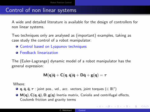
A wide and detailed literature is available for the design of controllers fornon linear systems.

Two techniques only are analysed as (important) examples, taking ascase study the control of a robot manipulator:

Control based on Lyapunov techniques

Feedback linearization

The (Euler-Lagrange) dynamic model of a robot manipulator has thegeneral expression:

M(q)q+ C(q, q)q+Dq+ g(q) = τ

Where:q, q, q, τ : joint pos., vel., acc. vectors, joint torques (∈ IR

n)

M(q),C(q, q),D, g(q) Inertia matrix, Coriolis and centrifugal effects,Coulomb friction and gravity terms

C. Melchiorri Control


Dynamic model of a 2 dof manipulator.

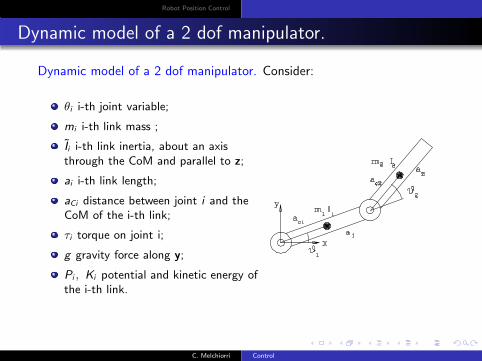
Dynamic model of a 2 dof manipulator. Consider:

θi i-th joint variable;

mi i-th link mass ;

Ii i-th link inertia, about an axisthrough the CoM and parallel to z;

ai i-th link length;

aCi distance between joint i and theCoM of the i-th link;

τi torque on joint i;

g gravity force along y;

Pi , Ki potential and kinetic energy ofthe i-th link.



Dynamic model of a 2 dof manipulator.

From M(q)q+ C(q, q)q+Dq+ g(q) = τ we have

M11θ1 +M12θ2 + c121θ1θ2 + c211θ2θ1 + c221θ22 + g1 = τ1

M21θ1 +M22θ2 + c112θ21 + g2 = τ2

or

[m1a2C1 +m2(a

21 + a2C2 + 2a1aC2C2) + I1 + I2]θ1 + [m2(a

2C2 + a1a

2C2C2) + I2]θ2

−m2a1aC2S2θ22 − 2m2a1aC2S2θ1θ2

+(m1aC1 +m2a1)gC1 +m2gaC2C12 = τ1

[m2(a2C2 + a1aC2C2) + I2]θ1 + [m2a

2C2 + I2]θ2

+m2a1aC2S2θ21

+m2gaC2C12 = τ2

Si ,Ci = sin(θi ), cos(θi ), Cij = cos(θi + θj)



Centralized control

Two important centralized control schemes are now introduced:

1 PD + gravity compensation

2 Inverse dynamics control



PD controller with gravity compensation

Given a desired reference configuration qd , the goal is to define acontroller ensuring the global asymptotic stability of the nonlineardynamical system (i.e the robot) described by:

M(q)q + C(q, q)q +Dq+ g(q) = u

For this purpose, let us define the error as

q = qd − q

and consider a dynamic system with state x given by

x =

[q

q

]

The direct Lyapunov method is exploited for the control law definition.




Let us consider the following candidate Lyapunov function

V (x) = V (q, q) =1

2qTM(q)q+

1

2qTKP q > 0 ∀ q, q 6= 0

where KP is a square (n × n) positive-definite matrix.

Function V (q, q) is composed by two terms:

1/2 qTM(q)qexpressing the kinetic energy of the system;

1/2 qTKP q

that can be interpreted as elastic energy stored by springs withstiffness KP ; these springs are a ‘physical interpretation’ of theposition control loops.




The reference configuration qd is constant. Then ˙q = −q, and the timederivative of V is:

V = qTMq+

1

2qTMq− q

TKP q

Since the robot dynamics can be rewritten as Mq = u−Cq−Dq− g, then

V = qTMq+

1

2qTMq− q

TKP q

= qT (u− Cq−Dq− g) +

1

2qTMq− q

TKP q

=1

2qT [M(q)− 2C(q, q)]q− q

TDq+ q

T [u− g(q)−KP q]

In order to compute the control input u, note that:

qT [M(q)− 2C(q, q)]q = 0 due to the structure of C (Christoffel symbols)

−qTDq is negative-definiteThus, by setting

u = g(q) +KP q

it is possible to guarantee that V is negative-semidefinite. In fact:

V = 0 q = 0, ∀q




The same result can be achieved also by adding a second term to thecontrol u:

u = g(q) +KP q−KD q

By defining KD as a positive-definite matrix, it results

V = −qT (D+KD)q

As a consequence, the convergence speed of the system to theequilibrium is increased.

Note that the terms KD q is equivalent to a derivative action in thecontrol loop (PD and gravity compensations).




KP Manipulator

KD

g(·)

❧❧❧✲ ✲ ✲ ✲✲✲

✛

❄

✻

✲

✻

✛

-

+

-

qd q uq

q

Remarks:

The control law is a linear PD controller with a nonlinear term (for gravitycompensation). The system is globally asymptotically stable for anychoice of KP , KD (positive-definite);

The derivative action is fundamental in systems with low friction effectsD. Typical examples are manipulators equipped with Direct Drive motors:the low electrical dumping in this case is increased by the control action(derivative actions).




The system evolves, and V decreases, as long as q 6= 0. Since V

does not depend on q (V = −qT (D+KD)q), it is not possible toguarantee that in steady state (when q = 0) also q = 0.

On the other hand, the steady state can be computed from thesystem equation

M(q)q+ C(q, q)q+Dq+ g(q)︸︷︷︸

Robot dynamics

= g(q) +KP q−KD q︸︷︷︸

PD+g(q)

In fact, in steady state (q = q = 0) it results

KP q = 0

that is (KP is positive definite):

q = qd

A perfect compensation of the gravity term g(q) is necessary,otherwise it is not possible to guarantee the stability of the system(robust control problem).



Inverse dynamics control

The manipulator is considered as a nonlinear MIMO system described by

M(q)q + C(q, q)q +Dq+ g(q) = u

or, in short: M(q)q + n(q, q) = u

The goal is now to define a control input u such that the overall systemcan be regarded as a linear MIMO system.

This result (global linearization) can be achieved by using a nonlinearstate feedback.It can be shown that this is possible because:

the model is linear in the control input u;

the matrix M(q) is invertible for any configuration of themanipulator.

Let us choose the control input u (based on the state feedback):

u = M(q)y + n(q, q)




By using the control input u defined as

u = M(q)y + n(q, q)

it follows that

Mq + n = My + n and thus (since M is invertible) → q = y

where y is the new input of the system.

M(q) Manipulator

n(q, q)

❤✲✲✲✻

✲✲

❄

✛✛

ss

∫ ∫✲ ✲ ✲y u

q

q

y q q❍❍✟✟




This is called an inverse dynamics control scheme because the inversedynamics of the manipulator must be calculated and compensated.

As long as yi affects only qi (yi = qi ), the overall system is linear anddecoupled with respect to y.

∫ ∫✲ ✲ ✲y q q

Now, it is necessary to define a control law y that stabilizes the system.By choosing

y = −KPq−KD q+ r

from q = y it follows

q+KD q+KPq = r

that is asymptotically stable if the matrices KP ,KD are positive-definite.




If matrices KP ,KD are diagonal matrices defined by

KP = diag{ω2ni} KD = diag{2δiωni}

the dynamics of the i-th component is characterized by the naturalfrequency ωni and by the damping coefficient δi .

A predefined trajectory qd (t) can be tracked by defining

r = qd +KD qd +KPqd

Then, the dynamics of the tracking error is:

¨q+KD˙q+KP q = 0

The error is not null if and only if q(0) 6= 0, ˙q(0) 6= 0 and converges tozero with a dynamics defined by KP ,KD .




M(q) Manipulator

n(q, q)

❤✲✲✲✻

✲✲

❄

✛✛

ssy u

q

q

❤

KP

KD❤

❤

✻

✻✲ ✲

❄

✲✲❅❅❘

��✒qd

qd

qd

˙q

q

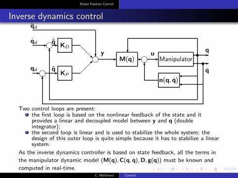
Two control loops are present:the first loop is based on the nonlinear feedback of the state and itprovides a linear and decoupled model between y and q (doubleintegrator);the second loop is linear and is used to stabilize the whole system; thedesign of this outer loop is quite simple because it has to stabilize a linearsystem.

As the inverse dynamics controller is based on state feedback, all the terms in

the manipulator dynamic model (M(q),C(q, q),D, g(q)) must be known and

computed in real-time.C. Melchiorri Control



This kind of controller has some implementation problems:

it requires the exact knowledge of the manipulator model (includingpayload, non-modeled dynamics, mechanical and geometricalapproximations, . . . );

the real-time computation of all the dynamic terms involved in thecontrol loop.

If, for computational reasons, only the principal terms are considered,then the control action cannot be precise due to the introducedapproximations. It follows that control techniques able to compensatemodeling errors are required:

Robust control (sliding mode, ...)

Adaptive control.



Inverse dynamics control - Example

Nonlinear system:

(2 + sin q)q + q3√1− 0.5 cos q +√

1 + q2 = u

Desired trajectory: trapezoidal velocity profile. kp = 100, kd = 14

0 1 2 3 4 5 6 7 8 9 100

20

40

60

80

100Posizione

0 1 2 3 4 5 6 7 8 9 10-3

-2

-1

0

1

2x 10

-3 Errore di Posizione

0 1 2 3 4 5 6 7 8 9 100

5

10

15

20Velocita‘

0 1 2 3 4 5 6 7 8 9 10-0.04

-0.02

0

0.02Errore di Velocita‘

0 1 2 3 4 5 6 7 8 9 10-5

0

5Accelerazione

0 1 2 3 4 5 6 7 8 9 10-0.2

0

0.2

0.4

0.6Errore di Accelerazione


Documents

NON LINEAR SYSTEMS: ANALYSYS AND CONTROL - unibo.it · AC&ST C. Melchiorri (DEI) Automatic Control & System Theory 2 Non linear systems Analysis and design methods based on the assumption