AAN113

1 AAN113 V1

Non-linear oscillation testing of viscoelastic fluids

LAOS: Large Amplitude Oscillatory Shear

Maik Novak, TA Instruments, Germany

Keywords: Non-linear Rheology, LAOS, Harmonics, Intensity ratios

(1)

From a molecular dynamical view the de-

formation within the LVR has to be amply

small or at least applied sufficiently slowly,

that the arrangement of the molecules is

never far from a thermodynamic equilib-

rium; the sample is not altered by the meas-

urement itself. To determine this maximum

tolerable, critical deformation is the aim of

a so-called strain sweep. A typical result is

shown in Fig. 2 for a 4 w% aqueous

solution of Xanthan Gum.

During such a strain sweep the amplitude

of the angular displacement is increased

stepwise at constant frequency, in this case

1 Hz, and the calculated dynamic moduli G´

and G˝ are plotted against the strain ampli-

tude. The linear viscoelastic region expands

in the shown example up to a strain of

about 15 %, characterized by moduli inde-

pendent of the strain amplitude. The left

image Fig. 3 proves that the waveforms of

both the excitation (strain) and the response

(stress) are simple sinusoids with the same

frequency. These two signals that are both

drawn with solid lines in Fig. 3 can be

differentiated just with the sufficient

information, that the stress always advances

the strain.

INTRODUCTION

In an oscillatory experiment a sinusoidal

strain or stress is applied to a sample of a

material under investigation while measur-

ing the respective answer of the sample.

The desired material function is then calcu-

lated from the transient signals. This mate-

rial function is called ―modulus‖ if the

stress is related to the strain or ―viscosity‖

in case of the stress being related to the

strain rate, whereas the ratio of strain to

stress has the character of a ―compliance‖.

Due to the delay between the excitation and

the response signals these material func-

tions are generally complex. As sketched in

Fig. 1 the transient stress * can be

decomposed into an elastic stress ´, in

phase with the deformation , and a viscous

stress ˝, in phase with the deformation rate

.

SAOS AND THE LINEAR VISCOELASTIC

REGION

Within the so-called linear viscoelastic

region (LVR) the response to a sinusoidal

excitation is again simply a sinusoid with

the same frequency, and moreover the ratio

of the amplitudes of input and output sig-

nals is independent of the amplitude of the

excitation, for example:

|γ*|const.|γ*|

||fG

.

2 AAN113 V1

|G*| =

=

G´ =

=

G˝ =

=

tan δ =

=

| *|/|γ*|

(G´2+G˝

2)

½

| ´|/|γ*|

(| *|/|γ*|) cos δ

| ˝|/|γ*|

(| *|/|γ*|) sin δ

| ˝|/| ´|

G˝/G´

Figure 1: Decomposition of the complex stress into an elastic and a viscous contribution and calculation of the respective moduli

Figure 2: Dynamic moduli obtained from a deformation sweep on a Xanthan Gum solution at constant frequency of 1 Hz. 50 mm-cone/plate system with 0.04 rad.

At larger strains a dependency of the

moduli on strain occurs in the given exam-

ple in such a way, that the storage modulus

G’ decreases, whereas the loss modulus G”

first increases and then decreases, like an

overshoot phenomenon. In literature this

transition from linear to non-linear behavior

is termed Type III [1]. From the shape of

the center and the right waveforms in Fig. 3

it is evident that the material’s response to a

still sinusoidal excitation cannot be

characterized by a sinusoidal function of the

same frequency any more; all the quantities

that are well known from the linear

viscoelastic theory, such as the complex

modulus |G*|, the storage modulus G´, the

loss modulus G˝ or even the loss factor tan

δ loose their physical meaning.

LAOS and the issue of quantifying non-

linear behavior

The stress response of a material to a sinu-

soidal strain with large amplitude is not

only composed of a contribution that oscil-

lates with the excitation frequency, but

shows also some higher frequencies, that

are invariably integer, neglecting edge ef-

fects yet odd multiples of the excitation fre-

quency. There is a quite simple reason for

only the odd numbers:

3 AAN113 V1

The viscosity of a material can only be an

even, symmetric function of the shear rate,

as the direction of the deformation has no

influence on the resistance against it:

(2)

The shear stress required for this deforma-

tion is the product of viscosity and shear

rate:

The shear rate in an oscillatory experiment

is the derivative of the strain with respect to

time:

(4)

and substituting (4) in (3) gives for the tran-

sient stress

(5)

The only odd powers of the cosines can be

converted [2] into

Substituting in Eq. (5) shows that only

odd multiples of the excitation frequency ω

contribute to the stress response. The mag-

nitudes of these contributions with higher

frequencies can be determined by either

cross-correlating the stress response against

sinusoids with odd multiples of the excita-

tion frequency or directly by a frequency

analysis called Fourier transformation [3 –

5]. The cross-correlation results in discrete

values for amplitudes and phase shifts of

the higher-frequent contributions, from the

Fourier transformation however spectra of

these quantities is obtained with more or

less distinct maxima of the intensities oc-

curring at the odd multiples of the excita-

tion frequency.

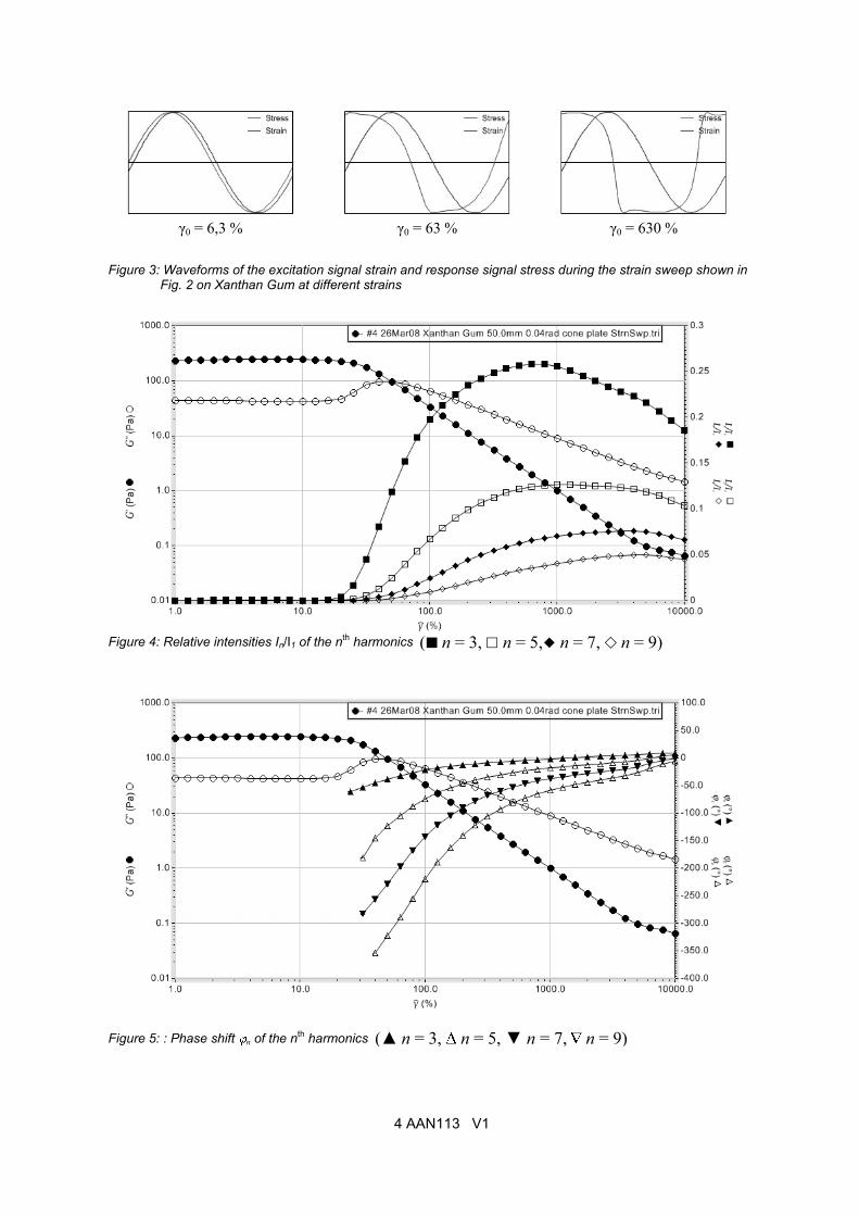
From the ratio of amplitudes of the higher

-frequent contributions to the amplitude of

the fundamental stress, i. e. that amount of

the stress oscillating with the excitation fre-

quency, so-called relative intensities In/I1 of

the nth harmonic can be derived, that are

plotted in Fig. 4. On leaving the LVR by

increasing strain amplitude to 15 % at first

the relative intensity of the third harmonics

() increases, at higher strains then also

those of the fifth (), seventh ( ) and ninth

( ◊ ) harmonics do. An explanation, e. g.

why the relative intensities exhibit a maxi-

mum, in order to discuss the material be-

havior, is at present a matter of research

[6 – 10].

Fig. 5 shows further the phase shifts n

between the nth harmonic and the funda-

mental stress, plotted as a function of the

strain amplitude. Within the LVR such a

phase shift is naturally pointless; its defini-

tion only acquires a foundation, as soon as

the respective higher-frequent contribution

has gained a significant intensity.

The following shall attempt to clarify, in

which way higher harmonics influence the

stress response and especially the shape of

their curves in the different means of

graphical representation. In order to keep

the number of parameters manageable, only

the influence of the third harmonic’s phase

shift 3 and that of the fundamental d1 at a

fixed relative intensity I3/I1 = 0.1 will be

discussed. Note: following the proposal of

Neidhöfer et al. [6] n denotes the phase

shift between the nth higher harmonics and

the fundamental stress, in contrast to the

phase shift 1 being the one between funda-

42 γγ)γη( cba

53

42

γγγ

γγγ

γ)γη()γσ(

cba

cba

t

tt

t

tt

ωcosω*γ

ωsin*γd

d

d

)(γdγ

tC

tBtAt

ωcos

ωcosωcosσ

5

3

N

n

n

N tnct

tttt

ttt

0

12

1615

413

ω)12cos(ωcos

ω5cosω3cos5ωcos10ωcos

ω3cosωcos3ωcos

(6)

4 AAN113 V1

γ0 = 6,3 % γ0 = 63 % γ0 = 630 %

Figure 3: Waveforms of the excitation signal strain and response signal stress during the strain sweep shown in Fig. 2 on Xanthan Gum at different strains

Figure 4: Relative intensities In/I1 of the nth harmonics ( n = 3, n = 5, n = 7, n = 9)

Figure 5: : Phase shift n of the nth harmonics (▲ n = 3, n = 5, ▼ n = 7, n = 9)

5 AAN113 V1

mental stress and the deformation, in ex-

actly the same way as the phase angle ,

which is well known from the theory of lin-

ear viscoelasticity.

WAVEFORMS

Fig. 6 shows the waveforms of the stress

for I3/I1 = 0.1 at various phase shifts 1 of

the fundamental and 3 of the third

harmonics versus the time, normalized with

the frequency, over one period of

oscillation. The open symbols indicate the

respective stress contributions, the filled

symbols represent the sum of them; both

are normalized with the amplitude of the

fundamental stress, while the deformation

3 = 0° 3 = 90° 3 = 180° 3 = 270°

1 = 0°

1 = 30°

1 = 60°

1 = 90°

Figure 6: : Waveforms of the stress for I3/I1 = 0.1 at various phase shifts

(solid line) is scaled with the strain

amplitude.

Generally the phase angle 3 lies between

0° and 360°, d 1 however only between 0°

and 90°, just as the „viscoelastic phase

shift― d. For 1 = 0° the fundamental stress

and the deformation are in-phase; without

any third harmonics this was an example of

ideally elastic behavior. The occurrence of

a third harmonics leads to a change in shape

of the stress wave, depending on the value

of the phase shift 3:

for 3 = 180° the stress wave gets

compressed vertically (—> square

wave)

for 3 = 190° the stress wave gets

distorted to the right (—> trailing

6 AAN113 V1

edge sawtooth wave)

for 3 = 180° the stress wave gets

stretched vertically (—> triangle

wave)

for 3 = 270° the stress wave gets

distorted to the left (—> leading

edge sawtooth wave)

LISSAJOUS FIGURES

Due to the fact that the phase shift 3 is

referred to the fundamental, the phase angle

d1 has no relevance for the shape of the cu-

mulative stress curve, whereas it has an in-

fluence on the well known Lissajous figures

shown in Fig. 7. Lissajous figures arise

from a superposition of harmonic

3 = 0° 3 = 90° 3 = 180° 3 = 270°

1 = 0°

1 = 30°

1 = 60°

1 = 90°

Figure 7: Lissajous-Bowditch figures for I3/I1 = 0.1 at various phase shifts

oscillations as plots of in this case the stress

against the strain. The shape of such a

Lissajous figure depends on the frequency

ratio and the phase difference at the

beginning of the oscillation. For equal

frequencies the figure is an ellipse with

varying eccentricity depending on the

phase. A line through the origin (open

symbols in the row for 1 = 0°) reveals the

limiting linear case of purely elastic

behavior, as the circle does for purely

viscous behavior (open symbols in the row

for 1 = 90°), provided an adequate scaling

of the properties with their respective

amplitudes. A general rule within the linear

viscoelastic region is, that the sine of the

(linear viscoelastic !) phase angle δ is the

7 AAN113 V1

positive value at the intersect of the Lissa-

jous curve with the normalized strain axis.

A Lissajous figures stays unchanged with

time, if the two frequencies involved have a

rational ratio, i. e. can be written as a

fraction of integer numbers; this is even

more the case, if only odd multiples of the

excitation frequency occur in the stress

response. But also the in the Lissajous-

Bowditch figures the effect of a third

harmonics and its phase angle 3 becomes

evident: the „viscoelastic basic shape― of an

ellipse gets distorted vertically. As the

parameter time is eliminated in this

representation, the Lissajous figures do not

contain further information, other that the

waveforms in Fig. 6. But during an

experiment it is convenient to monitor the

(at first transient) Lissajous figures

approaching a temporally stable pattern, in

order to evaluate, whether (or when) the

system has reached a quasi-steady state as

far as both the amplitudes or relative

intensities In/I1 and the phase shifts n are

concerned.

SIGNAL PROCESSING MY MEANS OF DIS-

CRETE FOURIER TRANSFORMATION AND

CROSS-CORRELATION

The (continuous) Fourier transformation

allows for expanding any continuous, even

a periodic process x(t) in a Fourier series

with the continuous spectrum X(ω):

(7)

As a rheometer samples the data signals at

discrete points in time, there is no continu-

ous function x(t) for the evaluation avail-

able, only a number M of measurements x

(m) of such a signal, that are each moni-

tored after time intervals Δt. The highest

frequency, that can be determined from

such a data set is the so-called Nyquist fre-

quency 1/(2×Δt) [11], which is exactly half

as large as the sampling rate [12]; the small-

est frequency is given by the inverse of the

tttxX d)iωexp()()ω(

overall measuring time M · Δt. All the dis-

crete frequencies with

(8)

contribute to the measurements x(m) = x

(m·Δt) with an amount of

(9)

The resulting frequency spectrum is usually

complex, even though the input values

might be real, as the transient signal has not

only an amplitude |X(k)|, but also a phase

shift k given by

(10)

with

For real input values x(m) the terms be-

tween the braces just vanish. Nevertheless

the effort in arithmetic operation lies in the

order of O(M2), as both k and m run through

all integer values from 1 to M /2 and 0 to M-

1, respectively. Therefore the so-called FFT

or „Fast Fourier Transformation has been

established especially for practical applica-

tions, as the arithmetic effort is „only― of O

(M·log M). Contrary to the direct calcula-

tion, the FFT uses intermediate data that

have already been calculated, thus saving

computational time. One of the prerequi-

sites for the FFT’s application is the num-

21with

π2ω

Mk

tM

kk

tM

kfk

1

0

2iexp)(

2

)ω(:)(

M

m

M

kmmx

M

kXkX

)(

)(arctan

)( 22

kX

kX

XXkX

k

1

0

22

1

0

22

sin)(cos)(2

)(

cos)(sin)(2

)(

M

m

M

km

imM

km

r

M

m

M

km

imM

km

r

mxmxM

kX

mxmxM

kX

8 AAN113 V1

ber of measurands M being a power of 2.

But as the number of data points recorded

during a measurement is free of choice, this

is no serious restriction. Without precisely

describing the literal algorithm of an FFT

(this can be found in the respective litera-

ture), the efficiency of an FFT can be dem-

onstrated with a thought example of the cal-

culation for M=1000 data points: a conven-

tional Fourier transformation with an effort

of O(M2) needs on the order of 1000·1000 =

103·103 = 106, i. e. one million calculations,

whereas an FFT with O(M·log M) reduces

this number down to just 1000·log(1000) =

1000·3 = 3000 ! The disadvantage of all the

Fourier methods is merely that the evalua-

tion can only be done subsequently, after all

the data have been saved and stored. In the

era of main memories measured in giga-

bytes and terabytes of hard disk sizes this

should not cause any issue. As additional

information the Fourier transformation de-

livers also values for the intensities between

the higher harmonics, enabling the quantifi-

cation of a signal-to-noise ratio with con-

clusions on the significance of the obtained

relative intensities.

The cross-correlation, an alternative for the

Fourier transformation, performs the

evaluation virtually in real time, but gives

no hint on the noise of the signal. Moreover

the data set has to comply with some

requirements to allow for the application of

this method. This is one of the major

differences between cross-correlation and

the Fourier transformation, even though the

mathematical operations themselves are

quite similar.

In signal analysis cross-correlation is a

measure of similarity of two waveforms as

a function of a time-lag applied to one of

them. Provided that the frequency of the

measurands is known (as in the case of a

stress response to a strain within the LVR),

both properties, stress and strain, can be

correlated with each a reference sine and a

reference cosine as follows:

(12)

The number M of measurands sampled

each in temporal lags Δt has to be chosen in

such a way, that the overall measuring time

M·Δt coincides with either exactly a quar-

ter, the half or an integer multiple of the

oscillation period. Meeting this requirement

is finally crucial for the accuracy of an

evaluation by cross-correlation.

The intensities and phase shifts of also the

higher harmonics can be determined with

exactly the same method of evaluation, as

they contribute in the same way with a

1

0

1

0

ωcosσ2

σ

ωsinσ2

σ

M

i

ii

M

i

ii

tM

tM

1

0

1

0

ωcosγ2

γ

ωsinγ2

γ

M

i

ii

M

i

ii

tM

tM

22 γγ*γ γ

γarctanδγ

22* arctanδ

*γ

**G γσ δδδ

Figure 8: Determination of the complex modulus and the (viscoelastic) phase shift from the discrete signals of stress and strain

9 AAN113 V1

known frequency to the response signal of

the stress. Therefore the signals are simi-

larly cross-correlated with reference waves

of odd integer multiples of the excitation

frequency:

(13)

with n = 1 for the fundamental and

n = 3, 5, 7,... for the 3., 5., 7.,... higher har-

monics. From these correlation either inten-

sities and phase shifts (related to the strain)

can be derived as

(14)

or relative intensities In/I1 and harmonic

phases in (related to the fundamental stress)

as:

(15)

Instead of these properties the so-called

Fourier coefficients Gn´ und Gn˝ can be de-

termined from the intensities and phase

shifts in Eq. (14), representing the stress

response in the time domain:

INTERPRETATION OF THE ADDITIONAL

PARAMETERS ON EXPLAINING A MATE-

RIAL’S BEHAVIOR

Hyaluronic acid (also called Hyaluronan)

is a glycosaminoglycan, consisting of up to

100,000 repeated disaccharide units (cf. Fig.

1

0

ωsinσ2

ωσ:σM

i

iin tnM

n

1

0

ωcosσ2

ωσ:σM

i

iin tnM

n

)(

22

n nInn

n

nn n arctan)(δ :δ

)(

)(/ 1

I

nIIIn

1δδ nnn

n

nn

n

nnnn

n

nn

tnGtnG

tntn

tnt

ωcosωsin*γ

ωcosδsinσωsinδcosσ

δωsinσ)(σ

(16)

9). Hyaluronan exhibits the ability to im-

bibe extremely large amounts of water re-

lated to its own mass (up to six liter water

per gram). The volume required by a hy-

drated hyaluronan molecule can be as much

as 10,000 times higher than that of the

molecule itself [13]. Hyaluronan is distrib-

uted widely throughout connective, epithe-

lial, and neural tissues and can satisfy many

requirements within the human body due to

the numerous and diverse chemico-physical

properties. The vitreous humor of the hu-

man eye for example consists of about 98 %

of water, bound to not more than 2 % of

hyaluronan. Vitreous humor is the clear gel

that fills the space between the lens and the

retina of the eyeball of humans and other

vertebrates. It is often referred to as the vit-

reous body or simply ―the vitreous". The

term ―Hyaluronic acid‖ itself is derived

from hyalos (Greek for vitreous) and uronic

acid because it was first isolated from the

vitreous humor and possesses a high uronic

acid content. Water, practically incom-

pressible, adds this property to any tissue

that contains hyaluronan; this makes it of

essential importance for the stability of con-

nective tissue, especially during the phase

of embryonic development, where rigid

structures have not been developed suffi-

ciently [14]. During a later stage of devel-

opment, when the ability of the skin to re-

pair itself by cell proliferation becomes less

and less effective, hyaluronan once more

gains of importance: this time for the

external application as a cosmetic skin care

product, or injected subcutaneously for

filling soft tissue defects such as facial

wrinkles. But also in the esthetic surgery

hyaluron based products are not only used

to plump up lips, but also for facial

reconstruction or even arthritic treatment

[14].

Figure 9: Structural unit of Hyaluronan

10 AAN113 V1

Furthermore hyaluronan can be found in

the Nucleus pulposus [15], the jelly-like

core of intervertebral (spinal) disks, where

it aids in distributing the hydraulic pressure

in all directions within each disc under

compressive loads, or as a main ingredient

in the synovial fluid, where it acts as a

natural lubricant and thus reduces the

friction between the articular cartilage and

other tissues in the joint to lubricate and

cushion them during movement [16]. The

conditions, under which hyaluronan has to

exhibit these as lubricating as damping

properties are certainly hard to compare

with those during a deformation within the

linear viscoelastic region between the

geometries of a rheometer; monitoring the

material’s response to extremely large

deformations is required: it all comes down

to LAOS.

Fig. 10 shows the result of a strain sweep

on a 1 w/w-% aqueous hyaluronan solution

at a frequency of 1 Hz. The linear

viscoelastic region, revealed by values for

storage modulus G´ () and loss modulus

G˝ ( ), that are independent on the

command strain amplitude, extends up to

deformations of about 60 %; at higher

strains the loss modulus decreases

significantly. The storage modulus remains

fairly constant up to approx. 100 %, and

decreases afterwards aswell. According to

[1] this behavior is typical for a transition

into the non-linear range of Type I. But

already at a strain of 25 % a significant

relative intensity I3/I1 of the third harmonics

() comes into play together with a related

harmonic phase φ3 (s). Higher harmonics

shall be neglected in this consideration.

The harmonic phase φ3 increases with the

strain from –90° (= 270°) up to 0° (= 360°).

From these values and the cognition of Fig.

6 the conclusion is straightforward, that the

waveforms of the stress response have to be

distorted to the left at small strains, while

getting more and more compressed with

increasing strain. The proof can be found in

Fig. 11; again stress and strain are plotted

indistinguishably with solid lines, but as

always the stress advances the strain.

Figure 10: Dynamic moduli, relative intensity I3/I1 and the corresponding phases from a strain sweep on a 1 w/w-%hyaluronan solution at constant frequency of 1 Hz. 40 mm on 50 mm parallel plates.

11 AAN113 V1

γ0 = 63 % γ0 = 630 % γ0 = 6300 %

I3/I1 = 0,44 % I3/I1 = 9,2 % I3/I1 = 23,2 %

φ3 =

=

–77,5°

282,5°

φ3 =

=

–47,0°

313,0°

φ3 =

=

–11,6°

348,4°

Figure 11: Waveforms of the command strain and the response stress during the strain sweep in Fig. 10 on hyaluronan .

The influence of the occurrence of higher

harmonics on a material’s behavior can nei-

ther be qualified, nor quantified by discuss-

ing the harmonic phase φ3; only the combi-

nation with the phase shift = 1 (◊) known

from the linear viscoelasticity between the

(fundamental) stress and the strain results in

the phase 3 ( ) related to the deformation

by rearranging Eq. (15.2):

(17)

The impact of the third higher harmonics

on the material behavior varying with the

magnitude of this effective phase angle 3

can be elucidated easily with the LAOS cir-

cle [17] in Fig. 12:

133 *3

Figure 11: The LAOS circle as graphical representation of the impact of a third higher harmonics on a material’s behavior

For waveforms shown in Fig. 11 the

effective phase 3 has the following values

3 = 89.5°

3 = 182.9°

3 = 257.3°

and allows accordingly the following inter-

pretation for the „application― in a knee

joint:

1. At ―small― strains, just outside the

LVR, 3 is about 90° and the mate-

rial shows with a quasi linear-elastic

behavior (comparable with the be-

havior within the LVR), while the

shear thickening, that accompanies

the onset of non-linearity, has a

rather stabilizing effect, for example

during standing still.

2. At ―large― strains of several 100

percent 3 is close to 180° and the

material acts linearly viscous,

though strain hardening, which

damps in a certain way the shocks

while bouncing or rope skipping.

3. At extremely large strains, that

might occur during running fast, 3

increases up to about 250°, so the

material doesn’t exhibit these hard-

ening or damping properties to still

the same degree, but rather acts

more shear thinning, in a sense of

lubricating, to reduce the friction

within the joint during movement.

12 AAN113 V1

LAOS – ALSO AN EXPERIMENTAL CHAL-

LENGE

Compared to measurement within the

LVR there are some more experimental as-

pects to consider in LAOS experiments,

which greatly influence the quality of the

results. Irrespective of the magnitude of the

strain amplitude the shape of the sample has

to be stable and uniform. Every occurrence

of edge fracture or swelling between the

geometries leads to erroneous measure-

ments in either case; but especially at large

strain amplitudes these failures might occur

at surprisingly low frequencies.

In the very first place the time is critical

for the sample to reach a steady state. In

LAOS experiments this time is much larger

than in the alternative experiments with

small strains. Usually 3 cycles for condi-

tioning of the sample are considered to be

sufficient in ordinary small strain experi-

ments, but at large strain amplitudes it may

take as long as 10 or more cycles, until the

sample reacts with a quasi-steady state re-

sponse in stress, as shown quite dramati-

cally in Fig. 13: During the first 60 seconds

the stress amplitude decreases from cycle to

cycle, only in the second half of the

experiment it reaches a constant value.

SUMMARY

Conventional oscillatory experiments with

comparably small deformations within the

linear viscoelastic region (SAOS = Small

Amplitude Oscillatory Shear) are usually

performed with the goal of characterizing a

material in a preferably well-defined state

of equilibrium, for example to obtain infor-

mation on the frequency dependent material

behavior. The deformation, which is in the

end imposed on the material, is very rarely

even of the same order of magnitude as the

strain a material is subjected to in the later

application. By means of oscillatory experi-

ments with ‖large― amplitude (LAOS =

Large Amplitude Oscillatory Shear) at least

a ―rheological finger print‖ if not a charac-

terization of the material can be obtained

under conditions that might be a bit closer

to those in reality. The representation of the

furthermore non-linear behavior can be

done in a graphical way

1. by means of waveforms, i. e. transient

curves of stress and strain, or

2. as Lissajous-Bowditch figures, where

the time is eliminated as parameter

and the stress is plotted as a function

of either the strain or the strain rate; a

Figure 13: Transient stress (t) and strain (t) in oscillation with = 1rad/s and | *| = 3000 % on a mixture of PVA/Borax

13 AAN113 V1

set of these figures dependent on fre-

quency and amplitude is then called

Pipkin diagram [18],

on the other hand a quantification of the

higher harmonics in the stress response on

a sinusoidal deformation is achievable by

indicating

3. the relative intensities, or intensity ra-

tios In/I1 and the harmonic phases n

related to the fundamental stress or

alternatively

4. the Fourier coefficients Gn´ und Gn˝

corresponding to the storage modulus

G´ and loss modulus G˝ from SAOS

experiments or analogously

5. the complex modulus |Gn*| together

with the phase n referred to the defor-

mation

of in each case the nth higher harmonics.

Irrespective of which representation might

be individually preferred, the number of

parameters will increase by two for each

and every higher harmonic taken into ac-

count; as it is not unlikely, to get up to 147

higher harmonics with sufficiently large

signal-to-noise ratios from a Fourier trans-

formation [19], there is plenty of room for

interpreting the influence of no fewer than

294 (!) more degrees of freedom on the be-

havior of a material under investigation.

REFERENCES

[1] Hyun, K., S. H. Kim, K. H. Ahn, S. J.

Lee (2002) Large amplitude oscilla-

tory shear as a way to classify the

complex fluids. J. Non-Newtonian

Fluid Mech 107: 51–65

[2] Bronstein, I. N., K. A. Semendjajew

(1987) Taschenbuch der Mathematik,

23. Aufl., B. G. Teubner, Leipzig

[3] Wilhelm, M., D. Maring, H. W. Spiess

(1998) Fourier-Transform Rheology.

Rheol. Acta 37: 399–405

[4] Wilhelm, M. (2002) Meth-

ods and apparatus for detecting

rheological properties of a material.

US patent 6,357,281

[5] Wilhelm, M. (2003) Methods and ap-

paratus for detecting rheological

properties of a material. EU patent 1

000 338

[6] Neidhöfer, T, M. Wilhelm, B. Deb-

baut (2003) Fourier-transform rheol-

ogy experiments and finite-element

simulations on linear polystyrene so-

lutions. J. Rheol 47(6):1351–1371

[7] Kallus, S., N. Willenbacher, S.

Kirsch, D. Distler, T. Neidhöfer, M.

Wilhelm, H. W. Spiess (2001) Charac-

terization of polymer dispersions by

Fourier transform rheology. Rheol

Acta 40: 552–559

[8] Langela M., U. Wiesner, H. W. Spi-

ess, M. Wilhelm (2002) Microphase

reorientation in block copolymer

melts as detected via rheology and 2D

SAXS. Macromolecules 35: 3198–

3204

[9] Ewoldt, R. H., C. Clasen, A. E. Hosoi,

G. H. McKinley (2006) Rheological

fingerprin­ting of gastropod pedal mu-

cus and bioinspired complex fluids for

adhesive locomotion. Soft. Matter 3:

634–643

[10] Vittorias, I., M. Parkinson, K. Klimke,

B. Debbaut, M. Wilhelm (2007) De-

tection and quantification of industrial

polyethylene branching topologies via

Fourier-transform rheology, NMR and

simulation using the Pom-pom model.

Rheol Acta 46: 321–340

[11] Shannon, C. E. (1949) Communica-

tion in the presence of noise. Proc.

IRE 37(1): 10–21. Nachdruck in:

Proc. IEEE 86(2), 1998

[12] Nyquist, H. (1928) Certain

topics in telegraph transmission the-

ory. Trans. AIEE 47:617–644. Nach-

druck in: Proc. IEEE 90(2), 2002

[13] http://de.wikipedia.org/wiki/

Glykosaminoglykane

[14] http://de.wikipedia.org/wiki/

Hyalurons%C3%A4ure

[15] http://flexikon.doccheck.com/

Nucleus_pulposus

[16] http://flexikon.doccheck.com/Synovia

14 AAN113 V1

[17] Franck, A. J., M. Nowak (2008) Non-

Linear Oscillation Testing with a

Separate Motor Transducer Rheome-

ter. XVth Int. Congr. Rheol., Monterey,

CA, USA

[18] Pipkin, A. C (1972) Lectures on Vis-

coelasticity Theory (Applied Mathe-

matical Sciences, Vol. 7), Springer-

Verlag, Berlin/Heidelberg/New York

[19] Wilhelm, M. (2008) New develop-

ments in mechanical characterization

of materials: FT-Rheology. Talk on

the occasion of the ARES-G2 presen-

tation in Karlsruhe on October, 14th

2008, organized by TA Instruments,

Germany.

Figure 14: A Tsunami – yet another wave with extremely large amplitude