Embed Size (px)
Citation preview
Deliverable D2.2-2.3
Non-linear force-displacement
performance
Luca Martinelli
Barbara Zanuttigh
Elisa Angelelli
Non-linear force-displacement performance
by
Luca Martinelli
Barbara Zanuttigh
Elisa Angelelli
Aalborg University
Department of Civil Engineering
Structural Design of Wave Energy Devices

Index
PREFACE ................................................................................................................................................................. 4
SHORT DESCRIPTION OF THE NUMERICAL MODEL ................................................................................... 4
CALIBRATION OF THE NUMERICAL MODEL ................................................................................................. 5
SIMPLE BUOY .................................................................................................................................................................. 6
DEXA DEVICE .............................................................................................................................................................. 13
LIMITATIONS OF THE MODEL ..........................................................................................................................37
SIMPLE MODEL OF THE MOORING SYSTEM ................................................................................................39
DESIGN OF OTHER MOORING SYSTEMS .......................................................................................................................... 42
EXAMINED WAVE CONDITIONS (15) .............................................................................................................................. 45
RESULTS ....................................................................................................................................................................... 46
NEW EXAMINED STRUCTURE ...........................................................................................................................51
MODELED GEOMETRY AND THE PROPOSED MOORING SYSTEM ...................................................................................... 51
EXAMINED WAVE CONDITIONS ...................................................................................................................................... 52
RESULTS ....................................................................................................................................................................... 53
CONCLUSIONS ............................................................................................................................................................... 54
OVERALL CONCLUSIONS ...................................................................................................................................56
REFERENCES .........................................................................................................................................................58

Preface
In agreement with the contract signed by “Dipartimento di Ingegneria Civile, Chimica, Ambientale e dei
Materiali” (DICAM), Bologna University - the Client - and by “Dipartimento di Ingegneria Civile Edile
Ambientale” (ICEA), Padova University – the Contractor - a numerical analysis has been performed on: i) a
simple buoy moored with a spread system formed by 4 chains; ii) the DEXA device moored with a spread
system of 8 chains and with a hinge between two interconnected elements.
Simulations have been carried out with the software ANSYS AQWA, made available by the Client.
The numerical model has been calibrated on the basis of experimental results, carried out by the Client.
After model calibration, three different systems have been tested: 1) a CALM system with the DEXA device
directly connected to the buoy; 2) a typical CALM system, with a cable connecting the buoy to the device; 3)
a different structure, with smaller dimensions.
Short description of the numerical model
ANSYS-AQWA software is an engineering analysis suite of tools for the investigation of the effects of
wave, wind and current on floating and fixed offshore and marine structures.
Two packages form the kernel of the simulations are used in this study:
i) ANSYS AQWA Diffraction,
ii) ANSYS AQWA Suite with Coupled Cable Dynamics.
The ANSYS AQWA Diffraction product develops the primary hydrodynamic variables required for complex
motions and response analyses, solving the Green function for irrotational flow by means of boundary
element and panel method (Newmann, 1985). Three-dimensional linear radiation and diffraction analysis
may be undertaken with multiple bodies, taking full account of hydrodynamic interaction effects that occur
between bodies. Computation of the second-order wave forces via the full quadratic transfer function
matrices (see for instance Journée and Massie, 2001) is apparently not fully working in the available
package.
The ANSYS AQWA Suite performs the dynamic analysis in either frequency or time domains, deriving the
impulsive response from the previous module and solving the equation of motion by means of the state-space
method (again, Journée and Massie, 2001). The analysis is coupled to the cable dynamics, where each line is
solved by a finite element approximation. Slow-drift effects (Newman, 1967; Chakrabarti, 2004) and
extreme-wave conditions may be investigated within the time domain, and damage conditions, such as line
breakage, may be included to investigate any transient effects that may occur.

The ANSYS AQWA portfolio of software solutions is part of the comprehensive set of applications from
ANSYS that collectively satisfy the design requirements of the offshore industry. Other alternative (but with
different approaches) software packages are for instance ASAS software for advanced structural assessment
of all types of fixed and floating structures, the Mechanical structural analysis tool, and FLUENT fluid
analysis.
Calibration of the numerical model
The first phase of this study aims at calibrating the numerical model and to gather some confidence on the
results.
Theoretically, the model does not contain specific variables to be calibrated, being all the variables and
parameters physically based.
In practice, however, it is essential to gather some confidence on the produced results, that are inaccurate for
very high and very low frequencies, for high and long waves in shallow waters, and with the simulated
geometry, that is necessarily a simplified version of the original, with a mesh of finite dimension.
In order to reach this goal, the numerical simulations reproduce as close as possible the tests carried out in
the deep-water basin of Aalborg University, within the MARINET project “Reliable design of mooring
system of Wave Energy Converters. Effects on device hydrodynamics and power performance”, as described
in the report MARINET-TA1-REDEM - proposal 32.
Two structures are analysed, a simple buoy and a model of the DEXA device.
Simple buoy
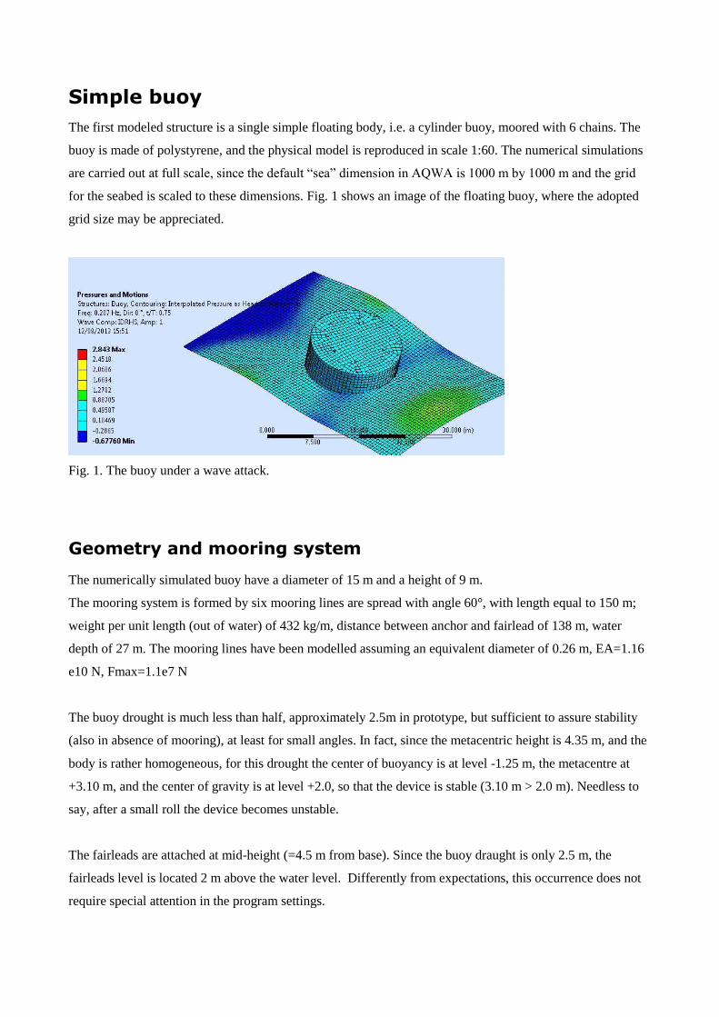
The first modeled structure is a single simple floating body, i.e. a cylinder buoy, moored with 6 chains. The
buoy is made of polystyrene, and the physical model is reproduced in scale 1:60. The numerical simulations
are carried out at full scale, since the default “sea” dimension in AQWA is 1000 m by 1000 m and the grid
for the seabed is scaled to these dimensions. Fig. 1 shows an image of the floating buoy, where the adopted
grid size may be appreciated.
Fig. 1. The buoy under a wave attack.
Geometry and mooring system
The numerically simulated buoy have a diameter of 15 m and a height of 9 m.
The mooring system is formed by six mooring lines are spread with angle 60°, with length equal to 150 m;
weight per unit length (out of water) of 432 kg/m, distance between anchor and fairlead of 138 m, water
depth of 27 m. The mooring lines have been modelled assuming an equivalent diameter of 0.26 m, EA=1.16
e10 N, Fmax=1.1e7 N
The buoy drought is much less than half, approximately 2.5m in prototype, but sufficient to assure stability
(also in absence of mooring), at least for small angles. In fact, since the metacentric height is 4.35 m, and the
body is rather homogeneous, for this drought the center of buoyancy is at level -1.25 m, the metacentre at
+3.10 m, and the center of gravity is at level +2.0, so that the device is stable (3.10 m > 2.0 m). Needless to
say, after a small roll the device becomes unstable.
The fairleads are attached at mid-height (=4.5 m from base). Since the buoy draught is only 2.5 m, the
fairleads level is located 2 m above the water level. Differently from expectations, this occurrence does not
require special attention in the program settings.
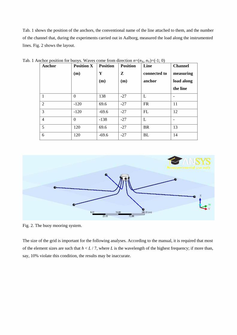
Tab. 1 shows the position of the anchors, the conventional name of the line attached to them, and the number
of the channel that, during the experiments carried out in Aalborg, measured the load along the instrumented
lines. Fig. 2 shows the layout.
Tab. 1 Anchor position for buoys. Waves come from direction n=(nX, nY)=(-1; 0)
Anchor Position X
(m)
Position
Y
(m)
Position
Z
(m)
Line
connected to
anchor
Channel
measuring
load along
the line
1 0 138 -27 L -
2 -120 69.6 -27 FR 11
3 -120 -69.6 -27 FL 12
4 0 -138 -27 L -
5 120 69.6 -27 BR 13
6 120 -69.6 -27 BL 14
Fig. 2. The buoy mooring system.
The size of the grid is important for the following analyses. According to the manual, it is required that most
of the element sizes are such that h < L / 7, where L is the wavelength of the highest frequency; if more than,
say, 10% violate this condition, the results may be inaccurate.

Examined conditions and results
In the laboratory, 8 wave states have been reproduced, as shown in

Tab. 2. The first thee wave conditions are considered to be “Ordinary”, the other are “Extreme”.
All the wave states (for both regular and irregular waves) were carried out considering three wave obliquities
0°, 15° and 30° in order to cover a wide range of dynamic loads on the moorings.
5 cases have been examined, for comparison with physical model tests, namely wave n. 3 with wave directed
at 0°, 15° and 30° obliquity, wave n. 7 and wave n. 8. The ordinary waves are expected to be correctly
simulated, whereas it is interesting to evaluate the quality of the simulation of the most extreme waves.
Results are stored in files given in Tab. 3.
Prior to the time domain analysis, the behaviour of the buoy under waves of different frequencies and
directions is required. Several results are obtained and processed by the timedomein analysis. An example is
the Ratio Amplitude Operator (RAO, ratio between the amplitude of the heave oscillation and the amplitude
of the incident wave), given in Fig. 3.
Fig. 3. The RAO of the buoy for heave oscillation.
Fig. 4 shows a typical response in terms of loads on the mooring lines.
Fig. 5 shows the characteristic load F1_20 of the most loaded chain vs the incident significant wave height
Hs, at prototype scale. It may be observed that the load does not increases significantly and that it does not
depend on the wave obliquity, as expected (due to symmetry). The origin of the axis is the initial pretention.
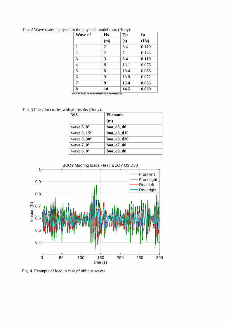
Tab. 2 Wave states analysed in the physical model tests (Buoy).
Wave n° Hs Tp fp
(m) (s) (Hz)
1 2 8.4 0.119
2 2 7 0.143
3 3 8.4 0.119
4 8 13.1 0.076
5 8 15.4 0.065
6 9 13.8 0.072
7 9 15.4 0.065
8 10 14.5 0.069
Tests in bold are simulated also numerically
Tab. 3 Files/directories with all results (Buoy).
WS Filename
(m)
wave 3, 0° boa_o3_d0
wave 3, 15° boa_o3_d15
wave 3, 30° boa_o3_d30
wave 7, 0° boa_o7_d0
wave 8, 0° boa_o8_d0
0 50 100 150 200 250 300
0.4
0.5
0.6
0.7
0.8
0.9
1BUOY Mooring loads - test: BUOY O3 D30
time (s)
ten
sio
n (
N)
Front left
Front right
Rear left
Rear right
Fig. 4. Example of load in case of oblique waves.

Comparison with experiments
Tab. 4 shows the obtained results in terms of mean, significant (Fsig) and maximum (Fmax) load along each
line. Data are also converted to model scale for easier comparisons (see also file Ris.xls).
The measured values are quite coherent among them. The initial value is nearly the same for all wave
attacks, since for each test the differences on the average are due to the presence of a small drift, that can
induce only a small change on the equilibrium position. Quantitatively, as also seen in Fig.4, the amplitude
of the load oscillations are significant but not extremely important, compatibly with absence of shock load.
The load increases with wave height (larger orbital excursions) but dynamic load decreases with the period,
and in fact the higher Fsig is found for WS n° 8 (=wave state 8) and the higher Fmax is found for WS n° 7
(shorter waves).
Experimental results are similar to the measured values for non-breaking conditions, and totally different for
extreme cases. For WS n° 3, where peak loads are not so relevant, the measured load corresponds to 270 kN,
the computed one to 188 kN, i.e. 70% of the measured one. In view of considerations that are presented in
the following sections, this small discrepancy is reasonably due to inaccuracy of the load cell readings.
In case of extreme waves (i.e. for WS n° 4,5,6,7,8) the high values of the measured forces on the mooring
system are due to the wave breaking near and/or on the device. The numerical model does not simulate this
event and as a consequence, whereas the max measured value for WS n° 8 corresponds to 5’700 kN at full
scale (breaking limit 11’000 kN), the highest simulated load is only 217 kN, i.e. 4% of the expected one.
Fig. 5. Simulated load (F 1_20) at full scale
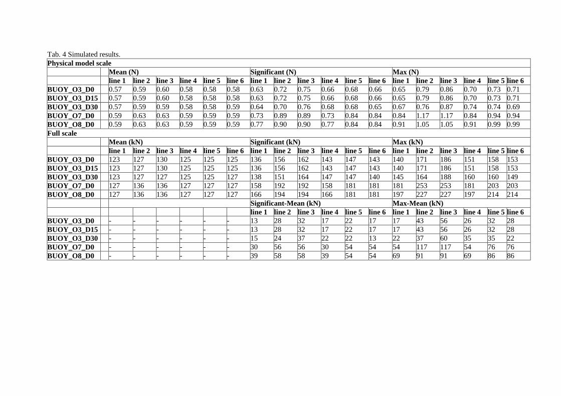
Tab. 4 Simulated results.
Physical model scale
Mean (N) Significant (N) Max (N)
line 1 line 2 line 3 line 4 line 5 line 6 line 1 line 2 line 3 line 4 line 5 line 6 line 1 line 2 line 3 line 4 line 5 line 6
BUOY_O3_D0 0.57 0.59 0.60 0.58 0.58 0.58 0.63 0.72 0.75 0.66 0.68 0.66 0.65 0.79 0.86 0.70 0.73 0.71
BUOY_O3_D15 0.57 0.59 0.60 0.58 0.58 0.58 0.63 0.72 0.75 0.66 0.68 0.66 0.65 0.79 0.86 0.70 0.73 0.71
BUOY_O3_D30 0.57 0.59 0.59 0.58 0.58 0.59 0.64 0.70 0.76 0.68 0.68 0.65 0.67 0.76 0.87 0.74 0.74 0.69
BUOY_O7_D0 0.59 0.63 0.63 0.59 0.59 0.59 0.73 0.89 0.89 0.73 0.84 0.84 0.84 1.17 1.17 0.84 0.94 0.94
BUOY_O8_D0 0.59 0.63 0.63 0.59 0.59 0.59 0.77 0.90 0.90 0.77 0.84 0.84 0.91 1.05 1.05 0.91 0.99 0.99
Full scale
Mean (kN) Significant (kN) Max (kN)
line 1 line 2 line 3 line 4 line 5 line 6 line 1 line 2 line 3 line 4 line 5 line 6 line 1 line 2 line 3 line 4 line 5 line 6
BUOY_O3_D0 123 127 130 125 125 125 136 156 162 143 147 143 140 171 186 151 158 153
BUOY_O3_D15 123 127 130 125 125 125 136 156 162 143 147 143 140 171 186 151 158 153
BUOY_O3_D30 123 127 127 125 125 127 138 151 164 147 147 140 145 164 188 160 160 149
BUOY_O7_D0 127 136 136 127 127 127 158 192 192 158 181 181 181 253 253 181 203 203
BUOY_O8_D0 127 136 136 127 127 127 166 194 194 166 181 181 197 227 227 197 214 214
Significant-Mean (kN) Max-Mean (kN)
line 1 line 2 line 3 line 4 line 5 line 6 line 1 line 2 line 3 line 4 line 5 line 6
BUOY_O3_D0 - - - - - - 13 28 32 17 22 17 17 43 56 26 32 28
BUOY_O3_D15 - - - - - - 13 28 32 17 22 17 17 43 56 26 32 28
BUOY_O3_D30 - - - - - - 15 24 37 22 22 13 22 37 60 35 35 22
BUOY_O7_D0 - - - - - - 30 56 56 30 54 54 54 117 117 54 76 76
BUOY_O8_D0 - - - - - - 39 58 58 39 54 54 69 91 91 69 86 86
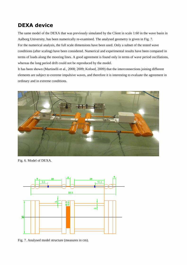
DEXA device
The same model of the DEXA that was previously simulated by the Client in scale 1:60 in the wave basin in
Aalborg University, has been numerically re-examined. The analysed geometry is given in Fig. 7.
For the numerical analysis, the full scale dimensions have been used. Only a subset of the tested wave
conditions (after scaling) have been considered. Numerical and experimental results have been compared in
terms of loads along the mooring lines. A good agreement is found only in terms of wave period oscillations,
whereas the long period drift could not be reproduced by the model.
It has been shown (Martinelli et al., 2008; 2009; Kofoed, 2009) that the interconnections joining different
elements are subject to extreme impulsive waves, and therefore it is interesting to evaluate the agreement in
ordinary and in extreme conditions.
Fig. 6. Model of DEXA.
Fig. 7. Analysed model structure (measures in cm).
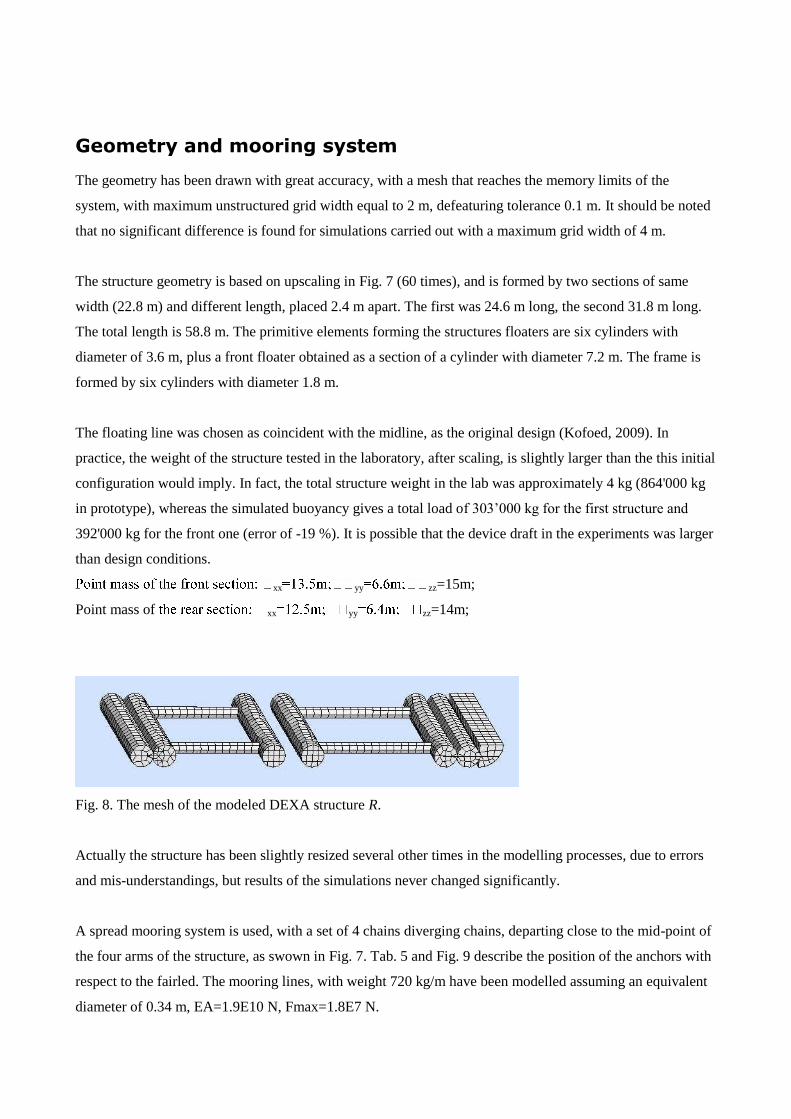
Geometry and mooring system
The geometry has been drawn with great accuracy, with a mesh that reaches the memory limits of the
system, with maximum unstructured grid width equal to 2 m, defeaturing tolerance 0.1 m. It should be noted
that no significant difference is found for simulations carried out with a maximum grid width of 4 m.
The structure geometry is based on upscaling in Fig. 7 (60 times), and is formed by two sections of same
width (22.8 m) and different length, placed 2.4 m apart. The first was 24.6 m long, the second 31.8 m long.
The total length is 58.8 m. The primitive elements forming the structures floaters are six cylinders with
diameter of 3.6 m, plus a front floater obtained as a section of a cylinder with diameter 7.2 m. The frame is
formed by six cylinders with diameter 1.8 m.
The floating line was chosen as coincident with the midline, as the original design (Kofoed, 2009). In
practice, the weight of the structure tested in the laboratory, after scaling, is slightly larger than the this initial
configuration would imply. In fact, the total structure weight in the lab was approximately 4 kg (864'000 kg
in prototype), whereas the simulated buoyancy gives a total load of 303’000 kg for the first structure and
392'000 kg for the front one (error of -19 %). It is possible that the device draft in the experiments was larger
than design conditions.
xx yy zz=15m;
Point mass of xx yy zz=14m;
Fig. 8. The mesh of the modeled DEXA structure R.
Actually the structure has been slightly resized several other times in the modelling processes, due to errors
and mis-understandings, but results of the simulations never changed significantly.
A spread mooring system is used, with a set of 4 chains diverging chains, departing close to the mid-point of
the four arms of the structure, as swown in Fig. 7. Tab. 5 and Fig. 9 describe the position of the anchors with
respect to the fairled. The mooring lines, with weight 720 kg/m have been modelled assuming an equivalent
diameter of 0.34 m, EA=1.9E10 N, Fmax=1.8E7 N.
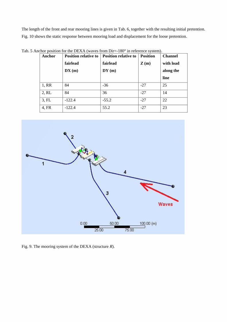
The length of the front and rear mooring lines is given in Tab. 6, together with the resulting initial pretention.
Fig. 10 shows the static response between mooring load and displacement for the loose pretention.
Tab. 5 Anchor position for the DEXA (waves from Dir=-180° in reference system).
Anchor Position relative to
fairlead
DX (m)
Position relative to
fairlead
DY (m)
Position
Z (m)
Channel
with load
along the
line
1, RR 84 -36 -27 25
2, RL 84 36 -27 14
3, FL -122.4 -55.2 -27 22
4, FR -122.4 55.2 -27 23
Fig. 9. The mooring system of the DEXA (structure R).
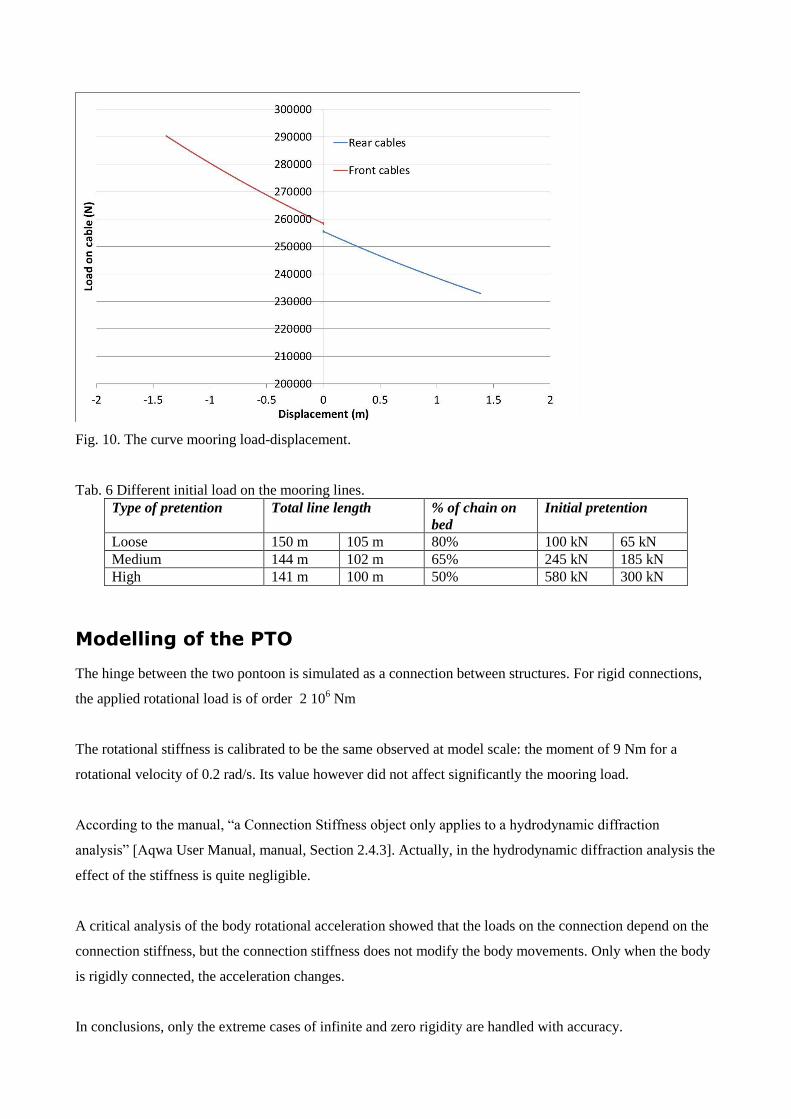
Fig. 10. The curve mooring load-displacement.
Tab. 6 Different initial load on the mooring lines.
Type of pretention Total line length % of chain on
bed
Initial pretention
Loose 150 m 105 m 80% 100 kN 65 kN
Medium 144 m 102 m 65% 245 kN 185 kN
High 141 m 100 m 50% 580 kN 300 kN
Modelling of the PTO
The hinge between the two pontoon is simulated as a connection between structures. For rigid connections,
the applied rotational load is of order 2 106 Nm
The rotational stiffness is calibrated to be the same observed at model scale: the moment of 9 Nm for a
rotational velocity of 0.2 rad/s. Its value however did not affect significantly the mooring load.
According to the manual, “a Connection Stiffness object only applies to a hydrodynamic diffraction
analysis” [Aqwa User Manual, manual, Section 2.4.3]. Actually, in the hydrodynamic diffraction analysis the
effect of the stiffness is quite negligible.
A critical analysis of the body rotational acceleration showed that the loads on the connection depend on the
connection stiffness, but the connection stiffness does not modify the body movements. Only when the body
is rigidly connected, the acceleration changes.
In conclusions, only the extreme cases of infinite and zero rigidity are handled with accuracy.

Wethervaning characteristics
In order to assess the wathervaning capabilities of this mooring setup, the DEXA (structure R) has been
subject to a set of regular wave conditions, with varying frequency and direction. The duration of the wave
attack is sufficient to reach a final equilibrium. For example, Fig. 12 shows the rotational yaw angle (in
degrees) of the front and rear structures (a definition of the yaw angle is given in Fig. 11). It may be observed
that the structure oscillates and reaches an equilibrium approximately after 300 s. Of course, a single line is
visible since the front and rear pontoon are constrained by the joint to assume the same direction.
Fig. 13 shows the yaw associated to varying wave obliquities. A sop=3.2% has been used, after noticing that,
as expected, for small wave heights (sop<0.2) the structure does not whethervanes significantly.
The result of this analysis is that:
- the structure whethervanes much less than expected for short waves.
- before an equilibrium is reached, the structure oscillates in yaw quite significantly, and it is possible
that it collides with adjacent structures.
- for obliquities larger than 45°, the structure does not whethervanes.
This result is important to guide the choice on the mooring system of the new structure to be designed.
Fig. 11. The six degrees of freedom.

Fig. 12. The jaw rotation of the device when subject to waves with 30° angle, T=4 s. Note that an asymptotic
value is reached after a few oscillations.
Fig. 13. The jaw rotation of the device when subject to waves with varying angle and frequency.
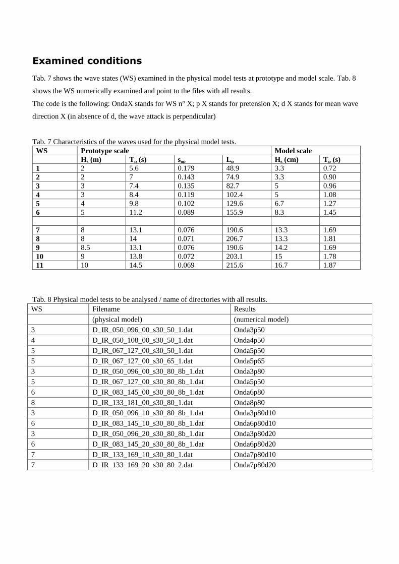
Examined conditions
Tab. 7 shows the wave states (WS) examined in the physical model tests at prototype and model scale. Tab. 8
shows the WS numerically examined and point to the files with all results.
The code is the following: OndaX stands for WS n° X; p X stands for pretension X; d X stands for mean wave
direction X (in absence of d, the wave attack is perpendicular)
Tab. 7 Characteristics of the waves used for the physical model tests.
WS Prototype scale Model scale
Hs (m) Tp (s) sop Lp Hs (cm) Tp (s)
1 2 5.6 0.179 48.9 3.3 0.72
2 2 7 0.143 74.9 3.3 0.90
3 3 7.4 0.135 82.7 5 0.96
4 3 8.4 0.119 102.4 5 1.08
5 4 9.8 0.102 129.6 6.7 1.27
6 5 11.2 0.089 155.9 8.3 1.45
7 8 13.1 0.076 190.6 13.3 1.69
8 8 14 0.071 206.7 13.3 1.81
9 8.5 13.1 0.076 190.6 14.2 1.69
10 9 13.8 0.072 203.1 15 1.78
11 10 14.5 0.069 215.6 16.7 1.87
Tab. 8 Physical model tests to be analysed / name of directories with all results.
WS Filename Results
(physical model) (numerical model)
3 D_IR_050_096_00_s30_50_1.dat Onda3p50
4 D_IR_050_108_00_s30_50_1.dat Onda4p50
5 D_IR_067_127_00_s30_50_1.dat Onda5p50
5 D_IR_067_127_00_s30_65_1.dat Onda5p65
3 D_IR_050_096_00_s30_80_8b_1.dat Onda3p80
5 D_IR_067_127_00_s30_80_8b_1.dat Onda5p50
6 D_IR_083_145_00_s30_80_8b_1.dat Onda6p80
8 D_IR_133_181_00_s30_80_1.dat Onda8p80
3 D_IR_050_096_10_s30_80_8b_1.dat Onda3p80d10
6 D_IR_083_145_10_s30_80_8b_1.dat Onda6p80d10
3 D_IR_050_096_20_s30_80_8b_1.dat Onda3p80d20
6 D_IR_083_145_20_s30_80_8b_1.dat Onda6p80d20
7 D_IR_133_169_10_s30_80_1.dat Onda7p80d10
7 D_IR_133_169_20_s30_80_2.dat Onda7p80d20
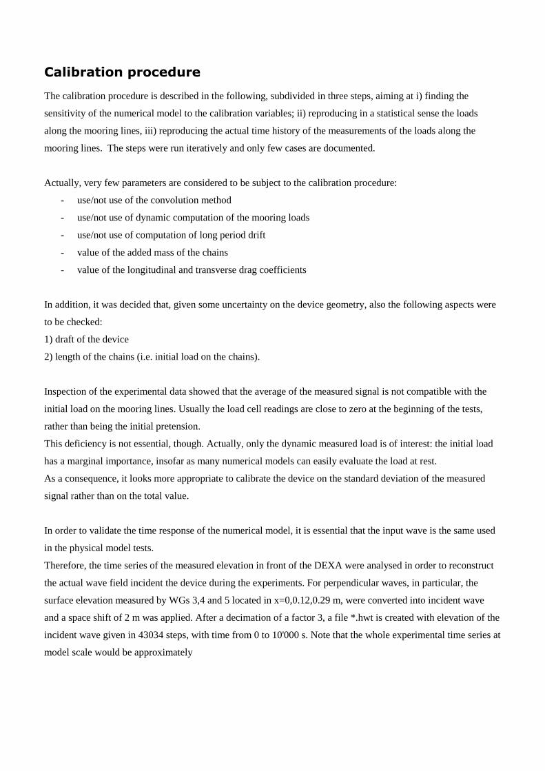
Calibration procedure
The calibration procedure is described in the following, subdivided in three steps, aiming at i) finding the
sensitivity of the numerical model to the calibration variables; ii) reproducing in a statistical sense the loads
along the mooring lines, iii) reproducing the actual time history of the measurements of the loads along the
mooring lines. The steps were run iteratively and only few cases are documented.
Actually, very few parameters are considered to be subject to the calibration procedure:
- use/not use of the convolution method
- use/not use of dynamic computation of the mooring loads
- use/not use of computation of long period drift
- value of the added mass of the chains
- value of the longitudinal and transverse drag coefficients
In addition, it was decided that, given some uncertainty on the device geometry, also the following aspects were
to be checked:
1) draft of the device
2) length of the chains (i.e. initial load on the chains).
Inspection of the experimental data showed that the average of the measured signal is not compatible with the
initial load on the mooring lines. Usually the load cell readings are close to zero at the beginning of the tests,
rather than being the initial pretension.
This deficiency is not essential, though. Actually, only the dynamic measured load is of interest: the initial load
has a marginal importance, insofar as many numerical models can easily evaluate the load at rest.
As a consequence, it looks more appropriate to calibrate the device on the standard deviation of the measured
signal rather than on the total value.
In order to validate the time response of the numerical model, it is essential that the input wave is the same used
in the physical model tests.
Therefore, the time series of the measured elevation in front of the DEXA were analysed in order to reconstruct
the actual wave field incident the device during the experiments. For perpendicular waves, in particular, the
surface elevation measured by WGs 3,4 and 5 located in x=0,0.12,0.29 m, were converted into incident wave
and a space shift of 2 m was applied. After a decimation of a factor 3, a file *.hwt is created with elevation of the
incident wave given in 43034 steps, with time from 0 to 10'000 s. Note that the whole experimental time series at
model scale would be approximately
Note that the file *.wht is a text file, to be imported as “irregular wave with slow drift”. The procedure used to
generate such file is given in the function GenerateWHT.m (FilenameToGenerated, Depth, WaveDirection,
Time, Eta)
Example of file with incident surface elevation (extension hwt).
DEPTH=27
G=9.806
DIRECTION=180
X_REF=0.0
Y_REF=0.0
NAME=ONDA5
CURRENT_SPEED=0
CURRENT_DIRECTION=0
0.10 -0.0453
0.20 -0.0397
0.30 -0.0341
etc. etc.
The starting point is the comparison of the numerical prediction (the initial “best guess”) to the measurements. In
particular, WS n° 5 has been selected, since the measured load has a very good signal to noise ratio, and waves
are not so large to induce breakings. The initial load on the cell has been tentatively removed by subtracting the
average before the comparison.
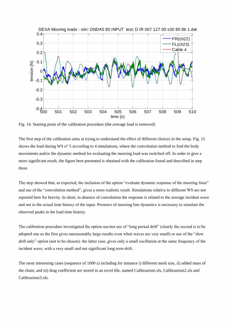
The results are somewhat different, both in shape and amplitude. Fig. 14 shows an example of comparison
relative to the front chains. The numerical results is symmetric, so that the load along cable 3 and 4 (see Fig. 9)
is the same, and only cable 3 is given in the legend for simplicity. Also the measured signal are similar between
them, and sometime show a double peak in correspondence with the maxima and minima, clearly induced by
dynamic effects. In the experimental data, oscillations in the time scale of the waveperiod are smaller than
predicted, and there is a long period drift, varying with time, that is absent in the simulations. The loads statistics
shows that the simulated chains are overestimated (the standard deviation ratio is 2.2).
500 501 502 503 504 505 506 507 508 509 510-0.4
-0.3
-0.2
-0.1
0
0.1
0.2
0.3
0.4
time (s)
ten
sio
n (
N)
DEXA Mooring loads - sim: ONDA5 80 INPUT test: D IR 067 127 00 s30 80 8b 1.dat
FR(ch22)
FL(ch23)
Cable 4
Fig. 14. Starting point of the calibration procedure (the average load is removed)
The first step of the calibration aims at trying to understand the effect of different choices in the setup. Fig. 15
shows the load during WS n° 5 according to 4 simulations, where the convolution method to find the body
movements and/or the dynamic method for evaluating the mooring load was switched off. In order to give a
more significant result, the figure here presented is obtained with the calibration found and described in step
three.
The step showed that, as expected, the inclusion of the option “evaluate dynamic response of the mooring lines”
and use of the “convolution method”, gives a more realistic result. Simulations relative to different WS are not
reported here for brevity. In short, in absence of convolution the response is related to the average incident wave
and not to the actual time history of the input. Presence of mooring line dynamics is necessary to simulate the
observed peaks in the load time history.
The calibration procedure investigated the option use/not use of “long period drift” (clearly the second is to be
adopted one as the first gives unreasonably large results even when waves are very small) or use of the “slow
drift only” option (not to be chosen): the latter case, gives only a small oscillation at the same frequency of the
incident wave, with a very small and not significant long term drift.
The most interesting cases (sequence of 1000 s) including for instance i) different mesh size, ii) added mass of
the chain, and iii) drag coefficient are stored in an excel file, named Calibrazioni.xls, Calibrazioni2.xls and
Calibrazioni3.xls.
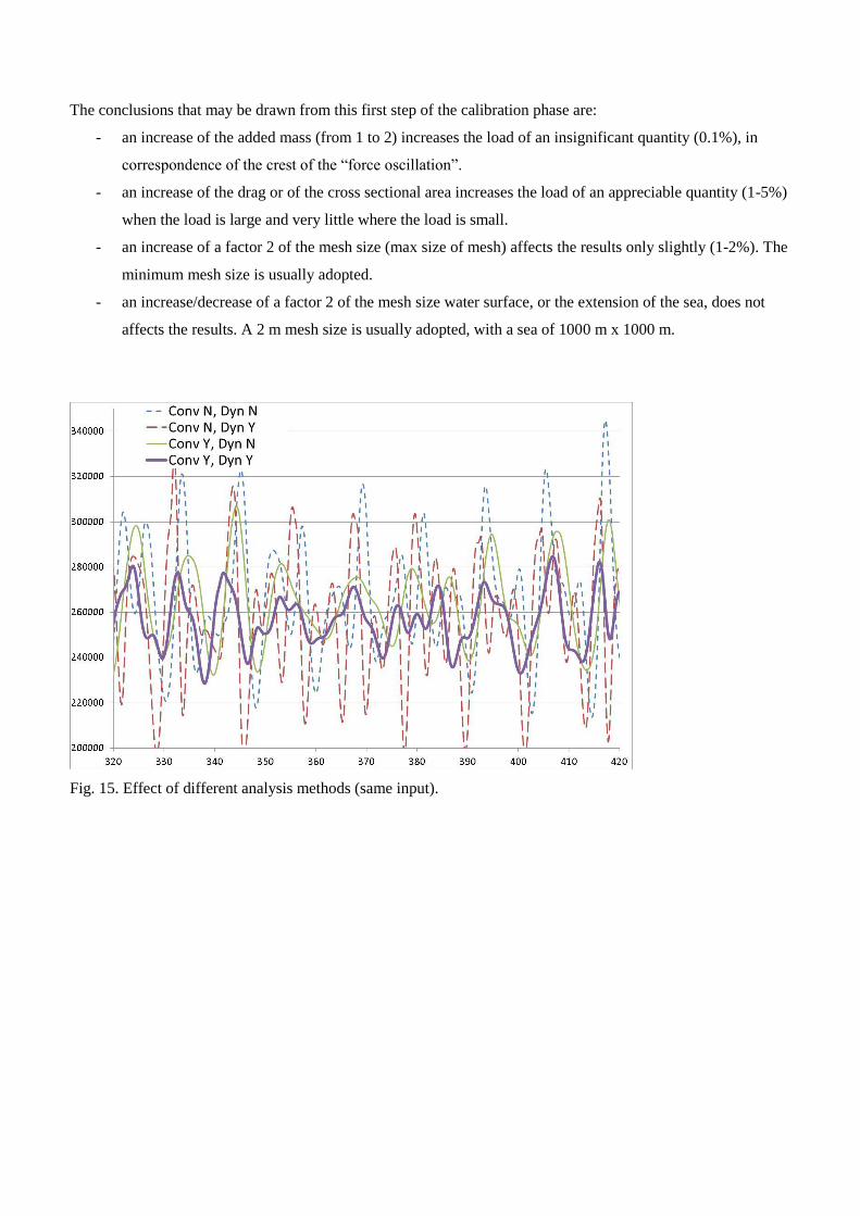
The conclusions that may be drawn from this first step of the calibration phase are:
- an increase of the added mass (from 1 to 2) increases the load of an insignificant quantity (0.1%), in
correspondence of the crest of the “force oscillation”.
- an increase of the drag or of the cross sectional area increases the load of an appreciable quantity (1-5%)
when the load is large and very little where the load is small.
- an increase of a factor 2 of the mesh size (max size of mesh) affects the results only slightly (1-2%). The
minimum mesh size is usually adopted.
- an increase/decrease of a factor 2 of the mesh size water surface, or the extension of the sea, does not
affects the results. A 2 m mesh size is usually adopted, with a sea of 1000 m x 1000 m.
Fig. 15. Effect of different analysis methods (same input).

Fig. 16. Effect of different analysis methods (doubled added mass and drag coefficient).
Tab. 9 Standard deviation of measured and simulated loads for WS n° 6, loose chains, perpendicular waves.
WS6/std of force (scaled to model unit) Front right
(ch23)
Front left (ch22) Rear right
(ch25)
Rear left
(ch23)
measured 0.061 0.080 0.038 0.047
Conv=Y, Dyn=Y, L=design, large mesh+ 0.045 0.033
Conv=Y, Dyn=Y, L=+0.5, large mesh+ 0.044 0.032
Conv=Y, Dyn=Y, L=+0.8, large mesh+ 0.043 0.031
Conv=Y, Dyn=Y, L=+1, large mesh+ 0.041 0.030
Conv=Y, Dyn=Y, L=102/145, lm+ 0.118 0.092
Conv=Y, Dyn=Y, L=104/147, lm+ 0.069 0.050
Conv=Y, Dyn=Y, L=104/148, lm+ 0.061 0.043
Conv=Y, Dyn=Y, L=104/148, use
frequency sum=Y, dt=0.02 s, lm+
0.061 0.043
Conv=Y, Dyn=Y, L=104/148, use frequency
sum=Y, DT=0.2 s, lm+
0.060 0.040
Conv=Y, Dyn=Y, L=104/148, No wave
damping=N, lm+
no change at all with above
Conv=Y, Dyn=N, L=design, large mesh+ 0.070 0.067
Conv=N, Dyn=N, L=design, large mesh+ 0.105 (note: errors for t>900 s) 0.078
Conv=N, Dyn=Y, L=design, large mesh+ 0.115 0.075
Conv=N, Dyn=Y, L=+1, large mesh+ 0.112 0.068
Conv=N, Dyn=Y, L=+3, large mesh+ 0.105 0.065
Conv=N, Dyn=Y, L=+111/155, lm+ 0.096 0.057
Conv=N, Dyn=Y, L=+116/159, lm+ 0.089 (note: slack cable) 0.054
Conv=N, Dyn=Y, L=design, fine mesh+ 0.119 (note: a few spikes) 0.070
+Large mesh: Max element size = 4 m; defeating tolerance = 0.1 m
Fine mesh: Max element size = 2 m; defeating tolerance = 0.1 m
The second step of the calibration aims at trying different configurations in order to achieve the same standard
deviation on the signals.
Tab. 9 reports part of the tested cases relative to WS n. 6, for which the results have been stored. The selected
case is the bold one in the list.
After this step, the comparison between measured and numerical results are better in average (the standard
deviation ratio is close to 1.0 rather than 0.75, first guess), but still not faithful in the details.
Note also that the ratio between the standard deviation of the load measured along the right and left chain is of
order 0.8, and this confirms that the first guess was already a good choice. It is anyway important to notice that
the standard deviation of the load on the right chains is systematically lower than that on the left ones, as if the
wave field was not fully homogeneous or the setup not symmetrical.
The third (and last) phase of the calibration process aims at calibrating the simulations so that the details of the
signals are reproduced at the best possible extent.
A sequence of tests focused on the difference settings: Use routine user force=Yes, Calculate CIF using added
mass=N, lengths of chains as in Tab. 10.
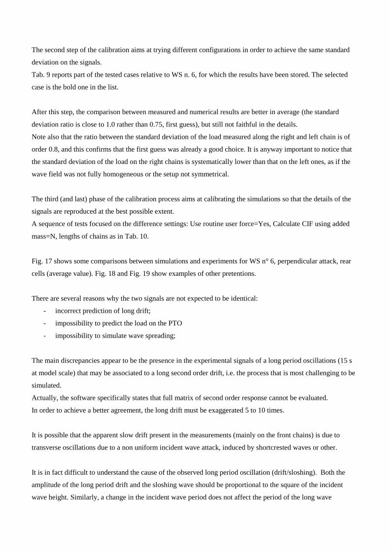
Fig. 17 shows some comparisons between simulations and experiments for WS n° 6, perpendicular attack, rear
cells (average value). Fig. 18 and Fig. 19 show examples of other pretentions.
There are several reasons why the two signals are not expected to be identical:
- incorrect prediction of long drift;
- impossibility to predict the load on the PTO
- impossibility to simulate wave spreading;
The main discrepancies appear to be the presence in the experimental signals of a long period oscillations (15 s
at model scale) that may be associated to a long second order drift, i.e. the process that is most challenging to be
simulated.
Actually, the software specifically states that full matrix of second order response cannot be evaluated.
In order to achieve a better agreement, the long drift must be exaggerated 5 to 10 times.
It is possible that the apparent slow drift present in the measurements (mainly on the front chains) is due to
transverse oscillations due to a non uniform incident wave attack, induced by shortcrested waves or other.
It is in fact difficult to understand the cause of the observed long period oscillation (drift/sloshing). Both the
amplitude of the long period drift and the sloshing wave should be proportional to the square of the incident
wave height. Similarly, a change in the incident wave period does not affect the period of the long wave

oscillation, regardless of its origin. Nevertheless, (as also shown in the following paragraph) the experiments do
not show a long period drift increasing with wave amplitude.
We should therefore conclude that the numerical model did not correctly evaluate the long drift (although the
option “computation of long period drift” is flagged).
15 20 25 30 35 40 45 50 55
-0.3
-0.2
-0.1
0
0.1
time (s)
ten
sio
n (
N)
DEXA Mooring load, test: Onda4p80
Front(ch22+ch23)/2
Rear(ch24+ch25)/2
Cable 1
Cable 3
Fig. 17. Comparison between simulated case and experiments, WS n° 6– pretention 80% (test
D_IR_083_145_10_s30_80_8b_1.dat).
24 26 28 30 32 34 36 38 40
-0.5
0
0.5
time (s)
ten
sio
n (
N)
DEXA Mooring load, test: Onda4p80
Front(ch22+ch23)/2
Rear(ch24+ch25)/2
Cable 1
Cable 3
Fig. 18. Comparison between simulated case and experiments, WS n° 4 – pretention 50% (test
D_IR_050_108_00_s30_50_1.dat).
20 25 30 35 40
-0.3
-0.2
-0.1
0
0.1
0.2
time (s)
ten
sio
n (
N)
DEXA Mooring load, test: Onda4p80
(ch24+ch25)/2
Cable 3
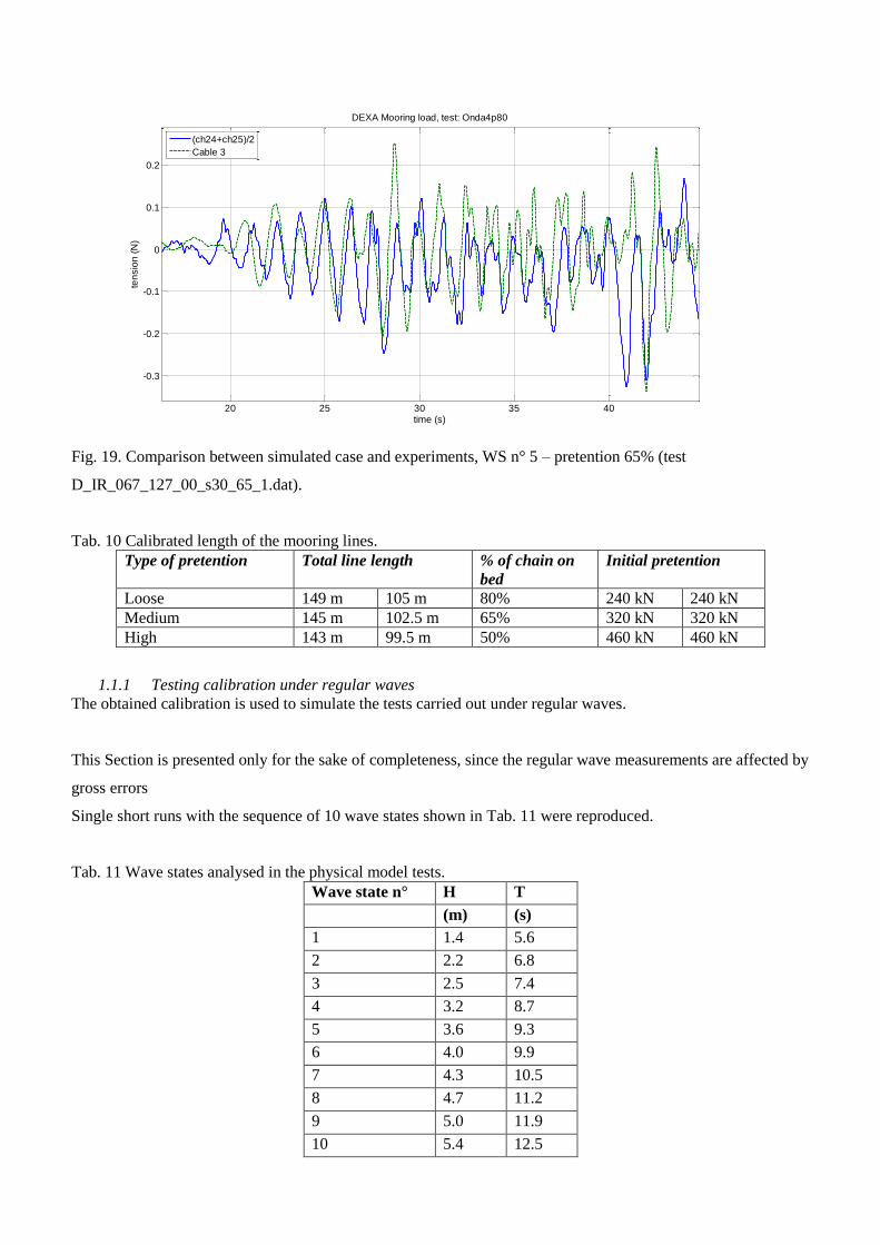
Fig. 19. Comparison between simulated case and experiments, WS n° 5 – pretention 65% (test
D_IR_067_127_00_s30_65_1.dat).
Tab. 10 Calibrated length of the mooring lines.
Type of pretention Total line length % of chain on
bed
Initial pretention
Loose 149 m 105 m 80% 240 kN 240 kN
Medium 145 m 102.5 m 65% 320 kN 320 kN
High 143 m 99.5 m 50% 460 kN 460 kN
1.1.1 Testing calibration under regular waves
The obtained calibration is used to simulate the tests carried out under regular waves.
This Section is presented only for the sake of completeness, since the regular wave measurements are affected by
gross errors
Single short runs with the sequence of 10 wave states shown in Tab. 11 were reproduced.
Tab. 11 Wave states analysed in the physical model tests.
Wave state n° H T
(m) (s)
1 1.4 5.6
2 2.2 6.8
3 2.5 7.4
4 3.2 8.7
5 3.6 9.3
6 4.0 9.9
7 4.3 10.5
8 4.7 11.2
9 5.0 11.9
10 5.4 12.5

In order to better simulate the long drift, the long drift oscillation was multiplied by a factor 5 to 10 and added to
the signal. This procedure gave much better results, as shown in Fig. 20.
Fig. 21 present the response to a series of regular waves of increasing wave state (from WS n° 1 to WS n° 10).
The difficulties of the calibration procedure become evident by the inspection of this signal: the measured
response does not agree with expectations with respect both to the long drift and to the to the load: in fact a large
drift is observed only for sea states 1 and 4. On the contrary, the measured signals show a constant load and a
long drift which does not increase with more intense sea states.
1880 1900 1920 1940 1960 1980 2000 2020-1
0
1
2
3
4x 10
4
time (s)
loa
d (
N)
loose mooring
Simulation
Measured
Fig. 20. Comparison between simulated case for regular wave and 10 times enhanced slow drift, WS n° 3.

0 2000 4000 6000 8000-2
0
2
4
6
8
10x 10
4
time (s)
loa
d (
N)
loose mooring
Simulation
Measured
Fig. 21. Comparison between simulated case for regular wave and x5 enhanced slow drift, all WS.
Model outputs
Results given by the solution of the hydrodynamic diffraction pattern are relative to the wave field and the RAO.
Fig. 22 shows the wave field around the structure as computed by the diffraction module, i.e. for regular waves
and separate unmoored floating devices. Fig. 23 shows the transmission and reflection characteristics for
different frequencies. Points are derived graphically, examining the flow field such as the one presented in Fig.
22.
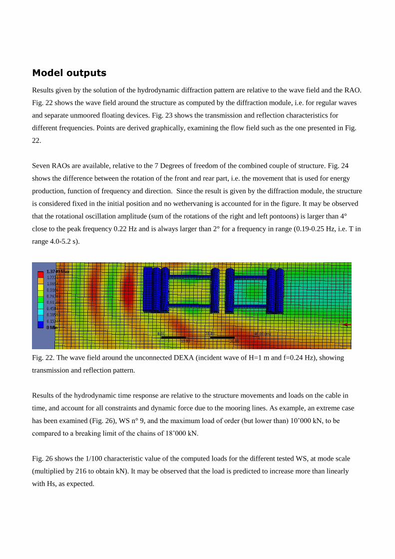
Seven RAOs are available, relative to the 7 Degrees of freedom of the combined couple of structure. Fig. 24
shows the difference between the rotation of the front and rear part, i.e. the movement that is used for energy
production, function of frequency and direction. Since the result is given by the diffraction module, the structure
is considered fixed in the initial position and no wethervaning is accounted for in the figure. It may be observed
that the rotational oscillation amplitude (sum of the rotations of the right and left pontoons) is larger than 4°
close to the peak frequency 0.22 Hz and is always larger than 2° for a frequency in range (0.19-0.25 Hz, i.e. T in
range 4.0-5.2 s).
Fig. 22. The wave field around the unconnected DEXA (incident wave of H=1 m and f=0.24 Hz), showing
transmission and reflection pattern.
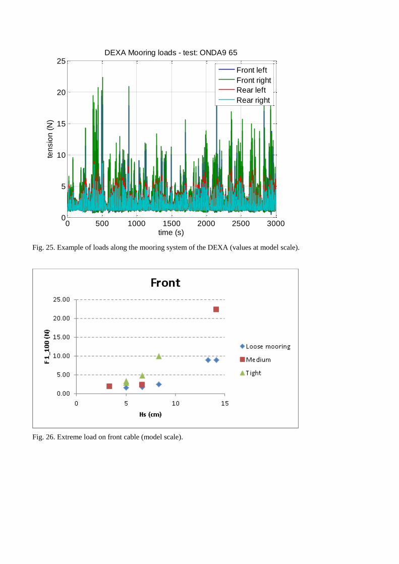
Results of the hydrodynamic time response are relative to the structure movements and loads on the cable in
time, and account for all constraints and dynamic force due to the mooring lines. As example, an extreme case
has been examined (Fig. 26), WS n° 9, and the maximum load of order (but lower than) 10’000 kN, to be
compared to a breaking limit of the chains of 18’000 kN.
Fig. 26 shows the 1/100 characteristic value of the computed loads for the different tested WS, at mode scale
(multiplied by 216 to obtain kN). It may be observed that the load is predicted to increase more than linearly
with Hs, as expected.
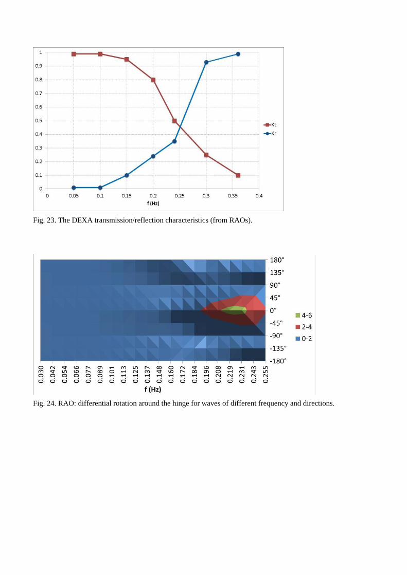
Fig. 23. The DEXA transmission/reflection characteristics (from RAOs).
Fig. 24. RAO: differential rotation around the hinge for waves of different frequency and directions.
0 500 1000 1500 2000 2500 30000
5
10
15
20
25DEXA Mooring loads - test: ONDA9 65
time (s)
ten
sio
n (
N)
Front left
Front right
Rear left
Rear right
Fig. 25. Example of loads along the mooring system of the DEXA (values at model scale).
Fig. 26. Extreme load on front cable (model scale).
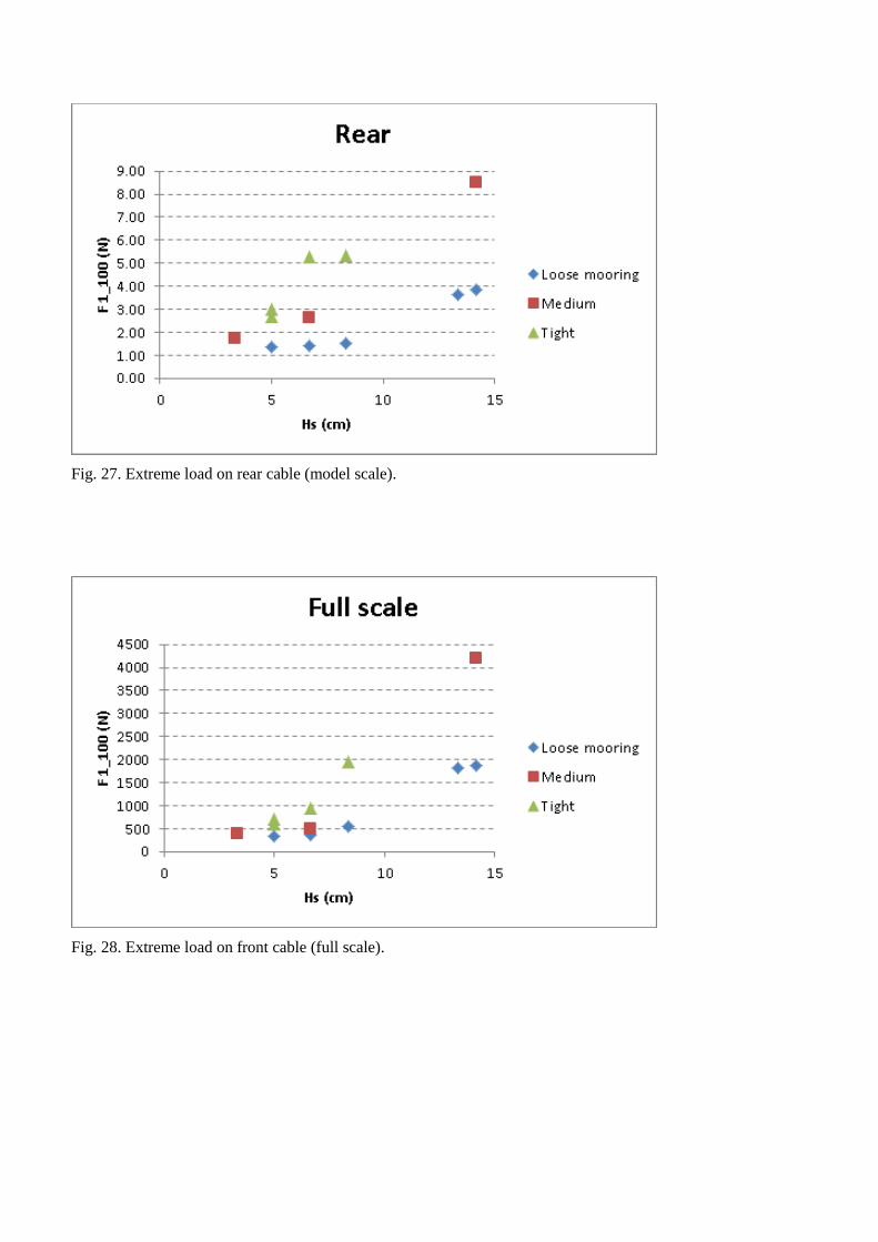
Fig. 27. Extreme load on rear cable (model scale).
Fig. 28. Extreme load on front cable (full scale).
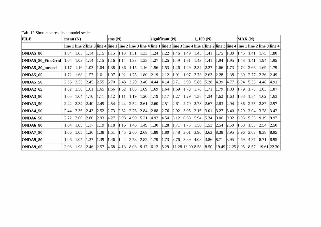
Tab. 12 Simulated results at model scale.
FILE mean (N) rms (N) significant (N) 1_100 (N) MAX (N)
line 1 line 2 line 3 line 4 line 1 line 2 line 3 line 4 line 1 line 2 line 3 line 4 line 1 line 2 line 3 line 4 line 1 line 2 line 3 line 4
ONDA5_80 1.04 1.03 1.14 1.15 1.15 1.13 1.31 1.33 1.24 1.22 1.46 1.49 1.45 1.41 1.75 1.80 1.45 1.41 1.75 1.80
ONDA5_80_FineGrid 1.04 1.03 1.14 1.15 1.16 1.14 1.33 1.35 1.27 1.25 1.49 1.51 1.43 1.41 1.94 1.95 1.43 1.41 1.94 1.95
ONDA5_80_noseed 1.17 1.16 1.03 1.04 1.38 1.36 1.15 1.16 1.56 1.53 1.26 1.29 2.34 2.27 1.66 1.73 2.74 2.66 1.69 1.79
ONDA5_65 1.72 1.68 1.57 1.61 1.97 1.92 1.75 1.80 2.19 2.12 1.91 1.97 2.73 2.63 2.28 2.38 2.89 2.77 2.36 2.49
ONDA5_50 2.66 2.55 2.45 2.55 3.70 3.48 3.20 3.40 4.44 4.14 3.71 3.98 5.86 5.28 4.39 4.77 6.04 5.33 4.48 4.91
ONDA2_65 1.62 1.58 1.61 1.65 1.66 1.62 1.65 1.69 1.69 1.64 1.69 1.73 1.76 1.71 1.79 1.83 1.79 1.75 1.83 1.87
ONDA3_80 1.05 1.04 1.10 1.11 1.12 1.11 1.19 1.20 1.19 1.17 1.27 1.29 1.38 1.34 1.62 1.63 1.38 1.34 1.62 1.63
ONDA3_50 2.42 2.34 2.40 2.49 2.54 2.44 2.52 2.61 2.60 2.51 2.61 2.70 2.78 2.67 2.83 2.94 2.86 2.75 2.87 2.97
ONDA4_50 2.44 2.36 2.43 2.52 2.73 2.62 2.73 2.84 2.88 2.76 2.92 3.05 3.16 3.01 3.27 3.40 3.20 3.04 3.28 3.42
ONDA6_50 2.72 2.60 2.80 2.93 4.27 3.98 4.90 5.31 4.92 4.54 6.12 6.68 5.94 5.34 9.06 9.92 6.03 5.35 9.19 9.97
ONDA6_80 1.04 1.03 1.17 1.19 1.18 1.16 1.46 1.49 1.30 1.28 1.71 1.75 1.58 1.53 2.54 2.50 1.58 1.53 2.54 2.50
ONDA7_80 1.06 1.05 1.36 1.38 1.51 1.45 2.60 2.68 1.88 1.80 3.48 3.61 3.96 3.63 8.38 8.95 3.96 3.63 8.38 8.95
ONDA9_80 1.06 1.05 1.37 1.39 1.46 1.42 2.73 2.82 1.79 1.73 3.76 3.89 4.08 3.86 8.71 8.95 4.69 4.37 8.71 8.95
ONDA9_65 2.08 1.98 2.46 2.57 4.68 4.13 8.03 9.17 6.12 5.29 11.28 13.00 8.58 8.50 19.49 22.25 8.95 8.57 19.61 22.30

Tab. 13 Simulated results at full scale.
FILE mean (kN) rms (kN) significant (kN) 1_100 (kN) MAX (kN)
line 1 line 2 line 3 line 4 line 1 line 2 line 3 line 4 line 1 line 2 line 3 line 4 line 1 line 2 line 3 line 4 line 1 line 2 line 3 line 4
ONDA5_80 225 222 245 248 248 244 282 288 269 264 315 321 312 305 379 389 312 305 379 389
ONDA5_80_FineGrid 225 222 247 249 251 247 287 291 274 269 321 327 309 305 420 421 309 305 420 421
ONDA5_80_noseed 253 250 222 225 298 293 247 251 338 331 272 278 506 491 358 373 593 575 365 387
ONDA5_65 372 363 339 347 426 414 378 389 472 457 412 425 589 569 493 515 623 597 510 538
ONDA5_50 574 551 530 552 799 751 692 735 959 895 801 859 1266 1139 948 1029 1304 1152 968 1060
ONDA2_65 350 341 349 357 358 349 357 366 364 355 365 373 379 370 387 396 387 378 396 404
ONDA3_80 227 224 237 240 242 239 256 260 257 253 275 279 299 290 350 352 299 290 350 352
ONDA3_50 524 505 519 537 548 528 544 563 563 541 563 584 601 577 612 634 618 595 620 642
ONDA4_50 528 509 525 544 590 566 589 614 623 596 631 658 683 650 706 734 692 657 709 739
ONDA6_50 588 561 605 632 922 859 1058 1146 1063 980 1323 1444 1283 1154 1956 2144 1303 1155 1984 2153
ONDA6_80 224 221 253 256 255 251 315 322 282 276 369 377 341 332 549 540 341 332 549 540
ONDA7_80 230 226 293 297 325 314 561 579 405 388 752 780 854 783 1810 1934 854 783 1810 1934
ONDA9_80 230 227 296 300 316 307 590 609 387 375 811 840 882 833 1881 1932 1013 944 1881 1932
ONDA9_65 450 427 531 555 1010 893 1734 1980 1323 1143 2437 2808 1852 1836 4210 4805 1933 1850 4235 4817
Conclusions
The DEXA model has been calibrated based on the experiments carried out at Alborg University. The calibration
procedure showed that the prediction should be based on the following options: convolution method on, dynamic
modelling of the cables on, waves with slow drift. Predictions are rather robust, and only large variations of the
physical parameters induce different results.
Calibration of was based on irregular wave tests. The initial load and the time history of the dynamic measured
signal is not perfectly reproduced by the numerical models.
The measured signal start from an incorrect assessment of the initial pretension, but this is not a limitation, being
a static load. It may be easily found by numerical models. What is most important to be evaluated experimentally
is the deviation from the average.
Actually, it is very common that measured load do not account for the initial pretention. That is because the
electrical drift of the load cells requires a periodic re-setting of the zero of the load cell, and this operation also
removes the initial load from the signal. No loss for the aim of the research, that focuses on information on the
dynamic load.
For the dynamic response, the issues to be considered are mainly two: i) the presence of a load on the PTO that
changes the body dynamics; ii) the presence of a large drift in the experiments.
As stated in the manual, it is not possible to include in the time domain simulations the presence of a stiff hinge.
This has important effects on the body dynamics. Similarly, only part of the long drift is correctly simulated (the
diagonal terms of the quadratic non-linear transfer function). Such approximations may be the cause for the large
discrepancy (5 to 10 times) between experiments and simulations.
For tests involving regular waves, measurements are considered to be not fully reliable. Predictions based on a
factor 5 or 10 amplification of the long drift are quite similar to the experiments, for WS n° 1 and 3. Apart from
the drift, results in general are reasonable in amplitude, but differ from experimental results. The load is anyway
predicted to increase more than linearly with Hs, as expected.
It is worthwhile noticing that the conceptual mooring system formed by 4 spread chains connected to the mid of
the 4 arms of the device, diverging from a single point forward of the center of gravity, has proved to be a sound
idea, but not optimal for all frequencies.
Limitations of the model
The model limitations may be divided into different groups, concerning: i) the simulated wave, ii) the simulated
processes, iii) the geometry, and iv) general bugs.
i) The main problems are related to the limitations in the modelling of the incident waves.
The model reproduces first order Airy waves. Regular and random Irregular waves are longcrested (1D). Oblique
waves are accepted. A short time history of wave elevation in a specified point may be defined: the duration of
the time history in the file is 7200s. This duration is necessary in order to give sufficient resolution of low
frequency resonant responses. The maximum number of timesteps is 150000, and this limits the series to
approximately 8-10’000 s. Wave direction during the sequence may not be modified.
ii) Some of the processes are not entirely simulated. Reflection and transmissions are only computed based on
the geometry initially under water, for waves of small amplitude. Overtopping is not really represented, although
the wave is seen to flow over the temporarily submerged body.
Wave drift loads are not exactly analysed, being a second order term quite difficult to compute except in deep
water. There are two contributions to this load: the hydrodynamic pressure due to the quadratic term in
Bernoulli’s equation acting on the submerged part of the construction and the contribution from wave action
around the still water level. Both these contributions are neglected when first order wave loads are estimated.
When second order are included, some error message appear (see bugs).
iii) The geometry is limited by the size of the mesh and by the defeaturing tolerance dimensions, that induces the
acceptable error (for instance a circle is seen as a polygon).
iv) A few bugs in the version 14.0 have been noticed.
- -The whole matrix with non-linear transfer functions is not solved (only the long period drift is
computed). A warning appears, and the computation carries on.
- In some cases, for some single frequencies, negative damping appears. Calculation for those frequencies
cannot be carried out, and the geometry or the mesh dimension must be modified.
- Modifications on the connection stiffness does induce a load along the connection, but unless a total
rigidity is obtained the movements of the body are not affected (i.e. the force along the connection is
computed but the information is not used for the calculation of the system dynamics, unless total rigidity
is obtained).
- -The wave obliquity is not considered when the waves are supplied in the user defined time histories.
Obliquity is always 0°, regardless of the actual value declared by the system.
- -Modification of the body geometry are not correctly accepted by the diffraction module: when the
diffraction module is started, the old geometry appears rather than the new, even after updating the
geometry.
- -Slight modifications of minor geometrical properties are recognised by the diffraction module but they
systematically induce a crash of the system during the meshing phase.
- -For each run, even if a single value of the input parameter is changed, the whole setup of several
Mbytes is stored.
- The AQWA-Gs does not open files if explorer is already open.
Simple model of the mooring system
The specific objective of this Section is to develop a simple procedure that allows to assess the load-
displacement curve of any of the mooring lines of the Dexa. The curve may then be used by other computational
tools focused on the evaluation of the body dynamics, coupled to the reaction of the power take off, but not
suited to evaluate the mooring load. It should be noted that the software does not seem to give theis curve as
output.
The simplest model may be described by a stiffness matrix. The matrix may be evaluated analytically as shown
by Leokogeorgaki et al (2005). This simple model is linear and it does not grasp the essence of the mooring
system behaviour, except in case of very small displacements.
The second step is a fairly good approximation of the quasi-static response. In some cases, this may be achieved
by solving the catenary equations, although this approach does not satisfy the “simplicity requirement” stated in
the objectives.
According to the analysed response of the DEXA, it is found that the vertical oscillations of the fairlead is
significantly lower than the wave amplitude, due to their position at mid length of the pontoon. Consequently, it
is reasonable to presume that the quasi-static load on the mooring only depends on the relative horizontal
position of the fairlead with respect to the anchor. This allows to relate the force to only two variables (x and y),
rather than three. The idea is in fact to fit a simple relation between force and position, based on a large set
information on these variables.
The set of data is obtained by AQWA simulations. Basically, the simulations should cover all the possible values
of axial force and fairlead displacements, compatibly with the constraints. In practice, it is sufficient that the
investigated range covers the possible positions reached during normal WEC operations.
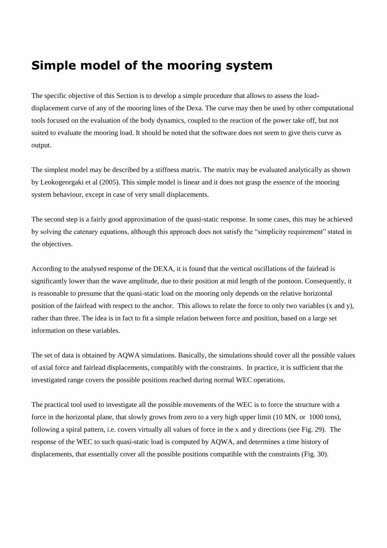
The practical tool used to investigate all the possible movements of the WEC is to force the structure with a
force in the horizontal plane, that slowly grows from zero to a very high upper limit (10 MN, or 1000 tons),
following a spiral pattern, i.e. covers virtually all values of force in the x and y directions (see Fig. 29). The
response of the WEC to such quasi-static load is computed by AQWA, and determines a time history of
displacements, that essentially cover all the possible positions compatible with the constraints (Fig. 30).
-1 -0.8 -0.6 -0.4 -0.2 0 0.2 0.4 0.6 0.8 1
x 106
-1
-0.8
-0.6
-0.4
-0.2
0
0.2
0.4
0.6
0.8
1x 10
6
Fx (N)
Fy (
N)
Fig. 29. Applied external load.
Fig. 30. Displacements of the fairleads.
In post-analysis, the displacements of the fairleads are related to their positions, or actually to the horizontal
distance between fairlead and anchor. Since there are two types of chains connected to the DEXA, it is obvious
that two relations are found. Note that the relation is not fully one to one. In fact, dynamic effects and possible

vertical oscillations will modify the details of the relation. Nevertheless, these details are quite unimportant as
the two figures show.
The fitting of the curve is necessary valid only in the investigated range. The two fittings are clearly visible in
the legend of the following figures, relative to the front and the rear chains.
In practice, the above relations allow to describe the mooring line response as required.
82 84 86 88 90 92 94 96 98 100100
200
300
400
500
600
700
800
Horizontal distance between fairlead and anchor (m)
Axia
l lo
ad
(kN
)
Chains, Lc=105 m
Computed
(F=2.2713*d'3-5.6663*d'
2+4.7224*d'-1.3128)*1e5 kN, d'=d/Lc
Fig. 31. Force-displacement curve for front chains.
126 128 130 132 134 136 138 140 142 144 146100
200
300
400
500
600
700
800
Horizontal distance between fairlead and anchor (m)
Axia
l lo
ad
(kN
)
Chains, Lc=150 m
Computed
(F=0.7059*d'3-1.8715*d'
2+1.6555*d'-0.4884)*1e6 kN, d'=d/Lc
Fig. 32. Force-displacement curve for rear chains.

Design of other mooring systems
Two structures have been analysed in this Section (among several that have been modelled):
a) Dexa with calm buoy, hanging chain
b) Dexa with calm buoy
The system is suited to a placement in array.
Modeled geometry and the proposed mooring system
The Dexa structure modelled in cases A and B is the same used for calibration, same depth (27 m), except that it
is moored to a buoy with diameter 12 m, draft 2 m and freeboard 2m (see Fig. 34). In order to limit the dynamic
movements of the buoy, the center of gravity is set at 2 m below the water surface.
xx yy zz=4.2m;
The Dexa is restrained with a long chain, necessary to avoid a rotation at 360° and provide a sort of extra
security connection in case the line breaks down. The anchor is placed 360 m away from the center of the buoy,
that is the minimum possible. The front tip of device is + 50 m away from the buoy.
The buoy at the vertex of a square, and the anchor of the rear chain at the opposite corner (Fig. 33), i.e 360 m
from the center of the buoy. The length of the rear chain is 262m, with weight 30 kg/m, equivalent diameter of
0.07 m, EA=0.8E9 N , Fmax = 8 E5 N.
The buoy is moored with 4 chains 67 m long, with anchors placed 60 apart. The mooring lines, with weight 720
kg/m have been modelled assuming an equivalent diameter of 0.34 m, EA=1.9E10 N, Fmax=1.8E7 N.
Actually, the system may benefit from a longer rear chain, since it would be less stretched, and a longer line
connecting the Dexa to the buoy, since there would be less risk of contact between these two structures. For a
cautious design, it is suggested that the overall distance is larger, of the order of 500 m. For instance, the side of
the square may be of order 6 times the length of the Dexa, and the distance between Dexa and buoy may be 1
length of the Dexa.
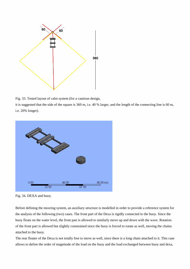
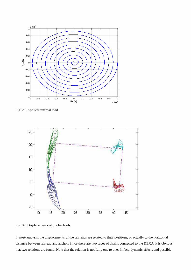
Fig. 33. Tested layout of calm system (for a cautious design,
it is suggested that the side of the square is 360 m, i.e. 40 % larger, and the length of the connecting line is 60 m,
i.e. 20% longer).
Fig. 34. DEXA and buoy.
Before defining the mooring system, an auxiliary structure is modelled in order to provide a reference system for
the analysis of the following (two) cases. The front part of the Dexa is rigidly connected to the buoy. Since the
buoy floats on the water level, the front part is allowed to similarly move up and down with the wave. Rotation
of the front part is allowed but slightly constrained since the buoy is forced to rotate as well, moving the chains
attached to the buoy.
The rear floater of the Dexa is not totally free to move as well, since there is a long chain attached to it. This case
allows to define the order of magnitude of the load on the buoy and the load exchanged between buoy and dexa,
that is essential to achieve convergence in the following step (of the order of 10 to 50kN for waves in the range 3
to 8 m).
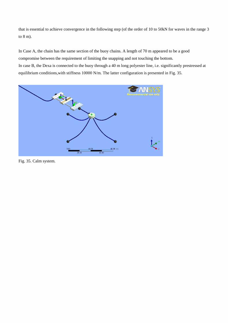
In Case A, the chain has the same section of the buoy chains. A length of 70 m appeared to be a good
compromise between the requirement of limiting the snapping and not touching the bottom.
In case B, the Dexa is connected to the buoy through a 40 m long polyester line, i.e. significantly prestressed at
equilibrium conditions,with stiffness 10000 N/m. The latter configuration is presented in Fig. 35.
Fig. 35. Calm system.

Examined wave conditions (15)
The examined wave conditions are WS from 3 to 8. Lower wave state produce loads on the chains too small,
loads for larger WS may be inaccurate due to the possible presence of breakers at the structure.
In order to analyse the effect of wave obliquity, the same wave state has been examined for different wave
obliquity, growing from 0 to 90°.
Tab. 14 Files/directories with all results.
Simulation WS Hs (m) Tp (s) Direction Directory storing data
(numerical model)
1 3 3 7.4 0° Calm_onda3
2 4 3 8.4 0° Calm_onda4
3 5 4 9.8 0° Calm_onda5
4 6 5 11.2 0° Calm_onda6
5 7 8 13.1 0° Calm_onda7
6 8 8 14.0 0° Calm_onda8
7 5 4 9.8 10° Calm_onda5_Dir10
8 5 4 9.8 20° Calm_onda5_Dir20
9 5 4 9.8 30° Calm_onda5_Dir30
10 5 4 9.8 40° Calm_onda5_Dir40
11 5 4 9.8 50° Calm_onda5_Dir50
12 5 4 9.8 60° Calm_onda5_Dir60
13 5 4 9.8 70° Calm_onda5_Dir70
14 5 4 9.8 80° Calm_onda5_Dir80
15 5 4 9.8 90° Calm_onda5_Dir80

Results
Results relative to Test A and B are presented by means of graphs and tables and some comments point out the
most interesting features.
Test A
The mooring system presents a critical element in the chain connecting the Dexa to the buoy. Actually, not all
sea states could be run, as the program aborts with error “time integration inaccuracy”. The problem probably
arise from the snapping that necessary occurs during the system dynamics.
Fig. 36. Sequence of images (Dt=0.1 s between images) showing the snapping event.
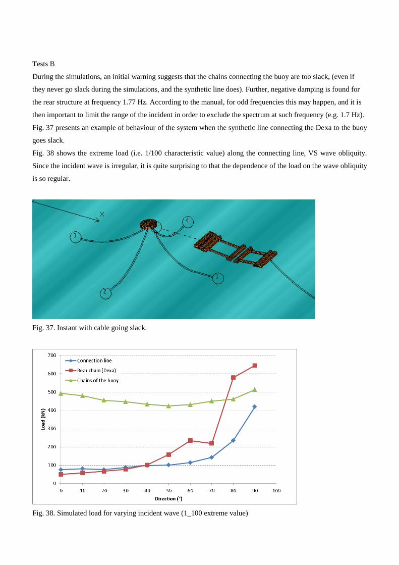
Tests B
During the simulations, an initial warning suggests that the chains connecting the buoy are too slack, (even if
they never go slack during the simulations, and the synthetic line does). Further, negative damping is found for
the rear structure at frequency 1.77 Hz. According to the manual, for odd frequencies this may happen, and it is
then important to limit the range of the incident in order to exclude the spectrum at such frequency (e.g. 1.7 Hz).
Fig. 37 presents an example of behaviour of the system when the synthetic line connecting the Dexa to the buoy
goes slack.
Fig. 38 shows the extreme load (i.e. 1/100 characteristic value) along the connecting line, VS wave obliquity.
Since the incident wave is irregular, it is quite surprising to that the dependence of the load on the wave obliquity
is so regular.
Fig. 37. Instant with cable going slack.
Fig. 38. Simulated load for varying incident wave (1_100 extreme value)

Tab. 15 Results of regular wave states.
Wave state
n°
H T Max vertical
displacement
Max load
(m) (s) (m) (kN)
1 1.4 5.6 0.2 450
2 2.2 6.8 0.8 480
3 2.5 7.4 1.1 450
4 3.2 8.7 1.4 510
5 3.6 9.3 1.5 560
6 4.0 9.9 1.8 680
7 4.3 10.5 1.9 930
8 4.7 11.2 2 1110
9 5.0 11.9 2.1 1140
10 5.4 12.5 2.4 1080
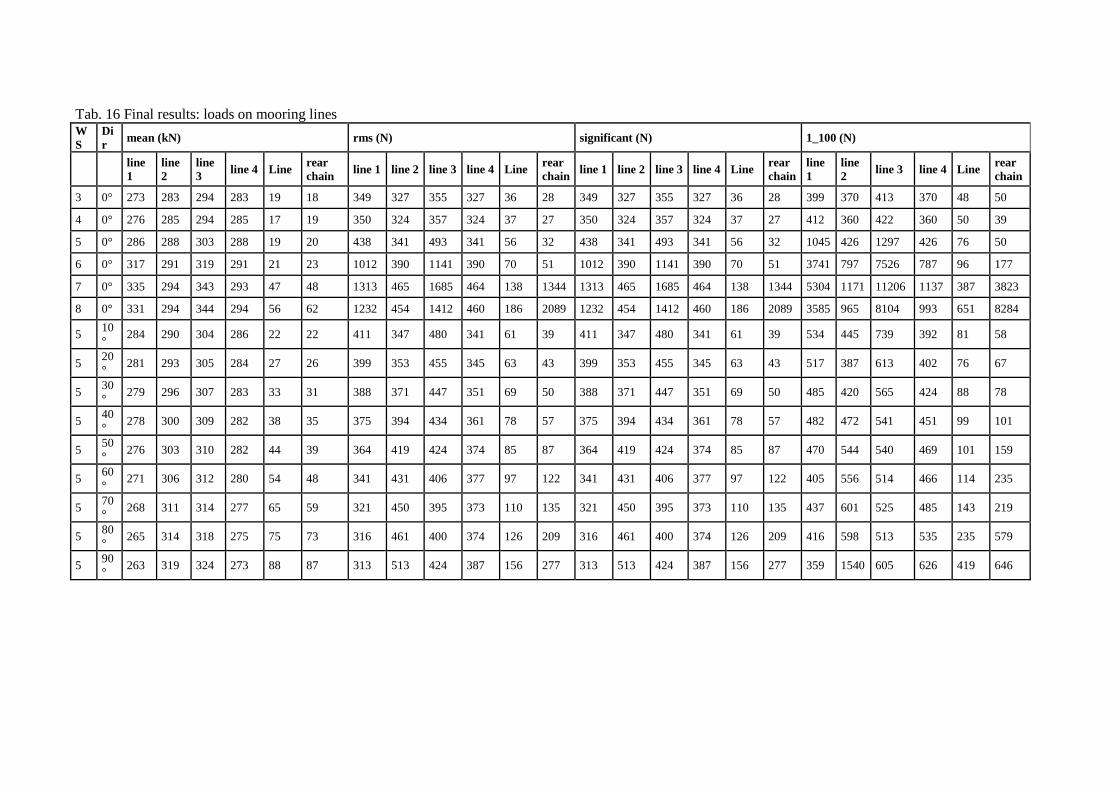
Tab. 16 Final results: loads on mooring lines W
S
Di
r mean (kN) rms (N) significant (N) 1_100 (N)
line
1
line
2
line
3 line 4 Line
rear
chain line 1 line 2 line 3 line 4 Line
rear
chain line 1 line 2 line 3 line 4 Line
rear
chain
line
1
line
2 line 3 line 4 Line
rear
chain
3 0° 273 283 294 283 19 18 349 327 355 327 36 28 349 327 355 327 36 28 399 370 413 370 48 50
4 0° 276 285 294 285 17 19 350 324 357 324 37 27 350 324 357 324 37 27 412 360 422 360 50 39
5 0° 286 288 303 288 19 20 438 341 493 341 56 32 438 341 493 341 56 32 1045 426 1297 426 76 50
6 0° 317 291 319 291 21 23 1012 390 1141 390 70 51 1012 390 1141 390 70 51 3741 797 7526 787 96 177
7 0° 335 294 343 293 47 48 1313 465 1685 464 138 1344 1313 465 1685 464 138 1344 5304 1171 11206 1137 387 3823
8 0° 331 294 344 294 56 62 1232 454 1412 460 186 2089 1232 454 1412 460 186 2089 3585 965 8104 993 651 8284
5 10
° 284 290 304 286 22 22 411 347 480 341 61 39 411 347 480 341 61 39 534 445 739 392 81 58
5 20
° 281 293 305 284 27 26 399 353 455 345 63 43 399 353 455 345 63 43 517 387 613 402 76 67
5 30
° 279 296 307 283 33 31 388 371 447 351 69 50 388 371 447 351 69 50 485 420 565 424 88 78
5 40
° 278 300 309 282 38 35 375 394 434 361 78 57 375 394 434 361 78 57 482 472 541 451 99 101
5 50
° 276 303 310 282 44 39 364 419 424 374 85 87 364 419 424 374 85 87 470 544 540 469 101 159
5 60
° 271 306 312 280 54 48 341 431 406 377 97 122 341 431 406 377 97 122 405 556 514 466 114 235
5 70
° 268 311 314 277 65 59 321 450 395 373 110 135 321 450 395 373 110 135 437 601 525 485 143 219
5 80
° 265 314 318 275 75 73 316 461 400 374 126 209 316 461 400 374 126 209 416 598 513 535 235 579
5 90
° 263 319 324 273 88 87 313 513 424 387 156 277 313 513 424 387 156 277 359 1540 605 626 419 646
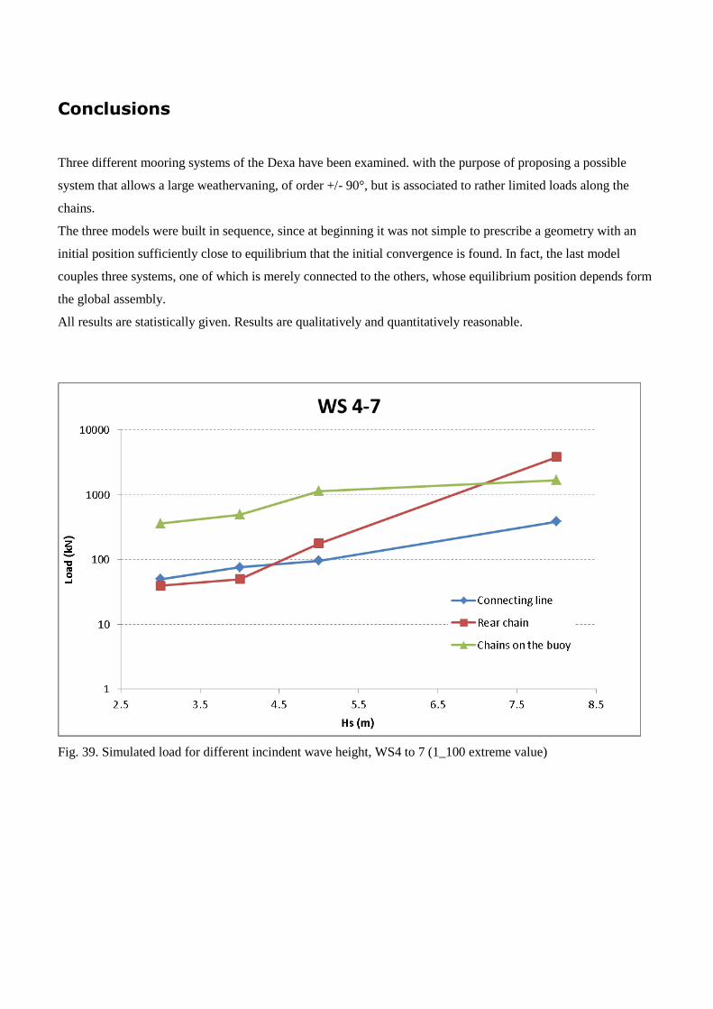
Conclusions
Three different mooring systems of the Dexa have been examined. with the purpose of proposing a possible
system that allows a large weathervaning, of order +/- 90°, but is associated to rather limited loads along the
chains.
The three models were built in sequence, since at beginning it was not simple to prescribe a geometry with an
initial position sufficiently close to equilibrium that the initial convergence is found. In fact, the last model
couples three systems, one of which is merely connected to the others, whose equilibrium position depends form
the global assembly.
All results are statistically given. Results are qualitatively and quantitatively reasonable.
Fig. 39. Simulated load for different incindent wave height, WS4 to 7 (1_100 extreme value)
New examined structure
In order to check the effect of the geometry on the results, the results of the physical model tests have been
compared to a new structure with slightly different dimensions. It was agreed that this may be the reason for the
observed discrepancies between calculated and measured loads.
Modeled geometry and the proposed mooring system
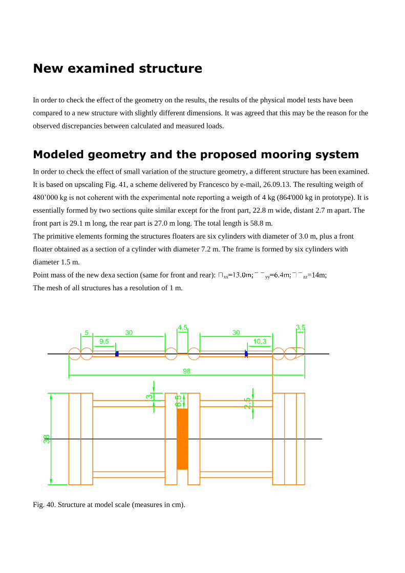
In order to check the effect of small variation of the structure geometry, a different structure has been examined.
It is based on upscaling Fig. 41, a scheme delivered by Francesco by e-mail, 26.09.13. The resulting weigth of
480’000 kg is not coherent with the experimental note reporting a weigth of 4 kg (864'000 kg in prototype). It is
essentially formed by two sections quite similar except for the front part, 22.8 m wide, distant 2.7 m apart. The
front part is 29.1 m long, the rear part is 27.0 m long. The total length is 58.8 m.
The primitive elements forming the structures floaters are six cylinders with diameter of 3.0 m, plus a front
floater obtained as a section of a cylinder with diameter 7.2 m. The frame is formed by six cylinders with
diameter 1.5 m.
Point mass of the new dexa section (same for front and rear): xx yy zz=14m;
The mesh of all structures has a resolution of 1 m.
Fig. 40. Structure at model scale (measures in cm).
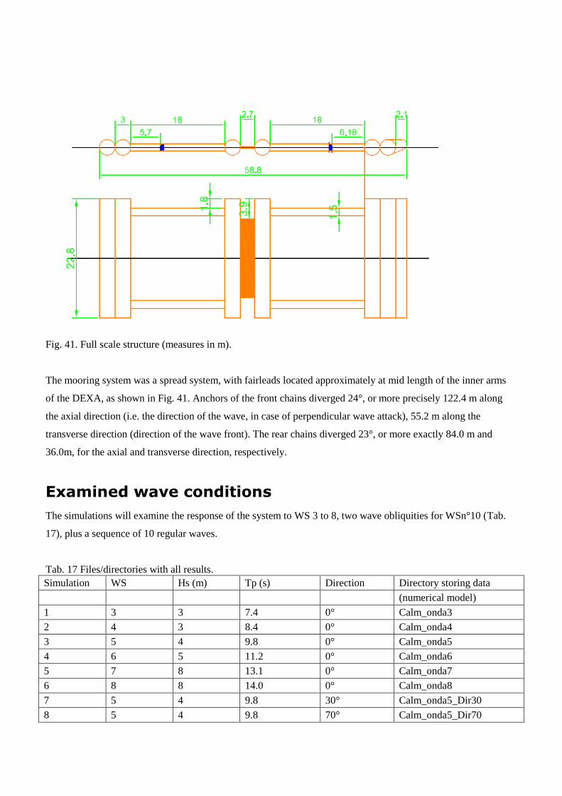
Fig. 41. Full scale structure (measures in m).
The mooring system was a spread system, with fairleads located approximately at mid length of the inner arms
of the DEXA, as shown in Fig. 41. Anchors of the front chains diverged 24°, or more precisely 122.4 m along
the axial direction (i.e. the direction of the wave, in case of perpendicular wave attack), 55.2 m along the
transverse direction (direction of the wave front). The rear chains diverged 23°, or more exactly 84.0 m and
36.0m, for the axial and transverse direction, respectively.
Examined wave conditions
The simulations will examine the response of the system to WS 3 to 8, two wave obliquities for WSn°10 (Tab.
17), plus a sequence of 10 regular waves.
Tab. 17 Files/directories with all results.
Simulation WS Hs (m) Tp (s) Direction Directory storing data
(numerical model)
1 3 3 7.4 0° Calm_onda3
2 4 3 8.4 0° Calm_onda4
3 5 4 9.8 0° Calm_onda5
4 6 5 11.2 0° Calm_onda6
5 7 8 13.1 0° Calm_onda7
6 8 8 14.0 0° Calm_onda8
7 5 4 9.8 30° Calm_onda5_Dir30
8 5 4 9.8 70° Calm_onda5_Dir70
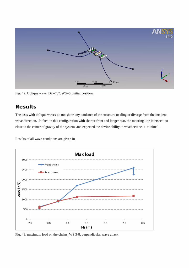
Fig. 42. Oblique wave, Dir=70°, WS=5. Initial position.
Results
The tests with oblique waves do not show any tendence of the structure to aling or diverge from the incident
wave direction. In fact, in this configuration with shorter front and longer rear, the mooring line intersect too
close to the center of gravity of the system, and expected the device ability to weathervane is minimal.
Results of all wave conditions are given in
Fig. 43. maximum load on the chains, WS 3-8, perpendicular wave attack
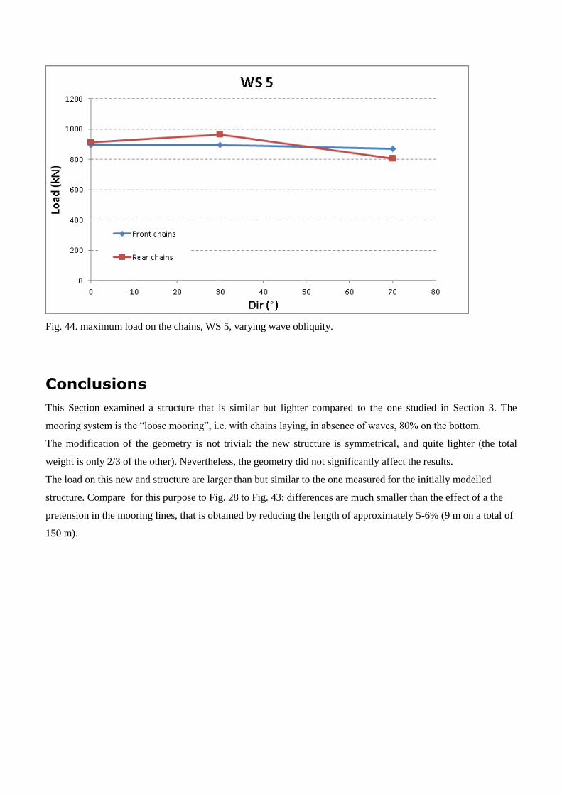
Fig. 44. maximum load on the chains, WS 5, varying wave obliquity.
Conclusions
This Section examined a structure that is similar but lighter compared to the one studied in Section 3. The
mooring system is the “loose mooring”, i.e. with chains laying, in absence of waves, 80% on the bottom.
The modification of the geometry is not trivial: the new structure is symmetrical, and quite lighter (the total
weight is only 2/3 of the other). Nevertheless, the geometry did not significantly affect the results.
The load on this new and structure are larger than but similar to the one measured for the initially modelled
structure. Compare for this purpose to Fig. 28 to Fig. 43: differences are much smaller than the effect of a the
pretension in the mooring lines, that is obtained by reducing the length of approximately 5-6% (9 m on a total of
150 m).
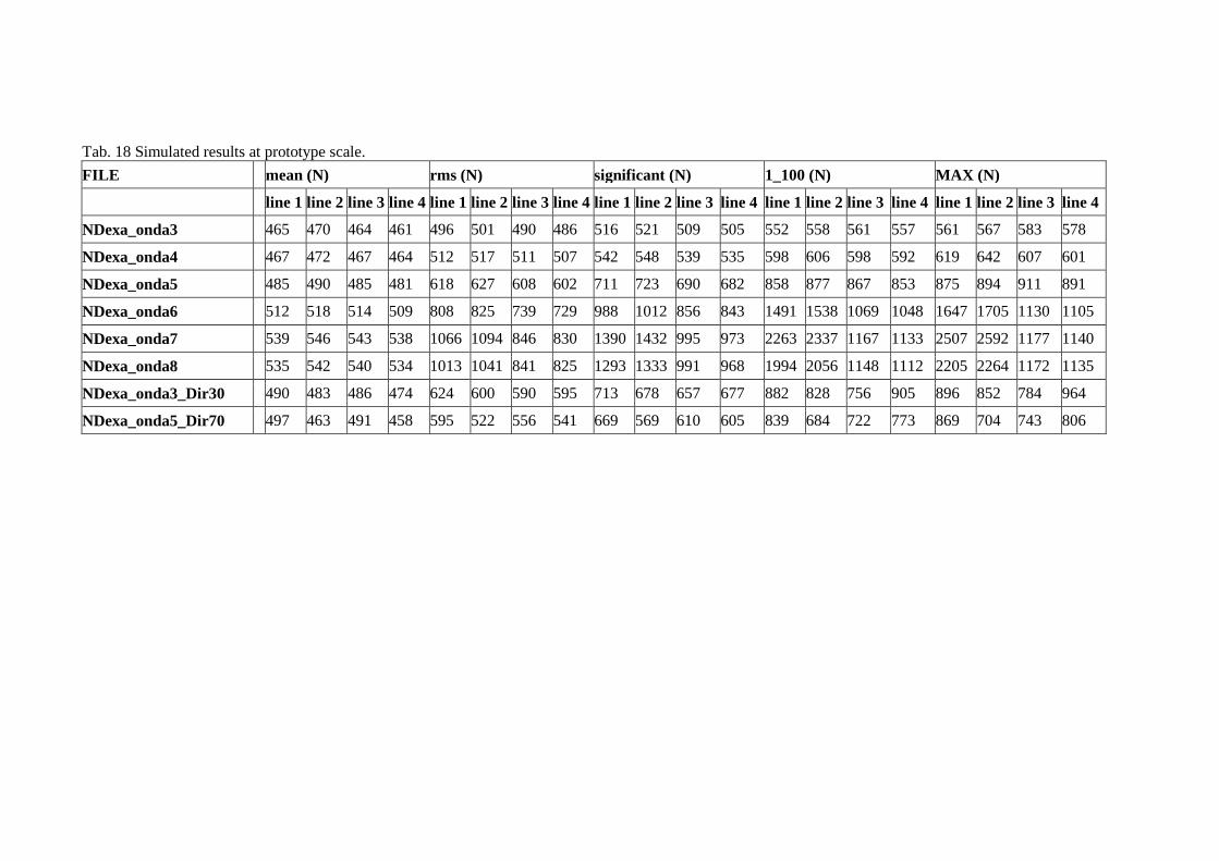
Tab. 18 Simulated results at prototype scale.
FILE mean (N) rms (N) significant (N) 1_100 (N) MAX (N)
line 1 line 2 line 3 line 4 line 1 line 2 line 3 line 4 line 1 line 2 line 3 line 4 line 1 line 2 line 3 line 4 line 1 line 2 line 3 line 4
NDexa_onda3 465 470 464 461 496 501 490 486 516 521 509 505 552 558 561 557 561 567 583 578
NDexa_onda4 467 472 467 464 512 517 511 507 542 548 539 535 598 606 598 592 619 642 607 601
NDexa_onda5 485 490 485 481 618 627 608 602 711 723 690 682 858 877 867 853 875 894 911 891
NDexa_onda6 512 518 514 509 808 825 739 729 988 1012 856 843 1491 1538 1069 1048 1647 1705 1130 1105
NDexa_onda7 539 546 543 538 1066 1094 846 830 1390 1432 995 973 2263 2337 1167 1133 2507 2592 1177 1140
NDexa_onda8 535 542 540 534 1013 1041 841 825 1293 1333 991 968 1994 2056 1148 1112 2205 2264 1172 1135
NDexa_onda3_Dir30 490 483 486 474 624 600 590 595 713 678 657 677 882 828 756 905 896 852 784 964
NDexa_onda5_Dir70 497 463 491 458 595 522 556 541 669 569 610 605 839 684 722 773 869 704 743 806
56
Overall conclusions
The numerical modelling gives a reasonable response, qualitatively and quantitatively in line with
expectations for non-breaking waves, but with details that are not exactly equal to measurements.
The order of magnitude of the obtained loads on the mooring is examined assuming that measurements did
not include the load at rest. Therefore only deviation from the mean of the measured and computed loads is
compared. Comparison is satisfactory, within a 20% discrepancy, but for large and breaking waves, the
numerical model over-predicts the measurements. Actually, measurements do not grow according to
expectations, whereas the model gives a reasonable result.
The discrepancy between simulations and experiments may well be explained by the model limitations on
the one side, and by measurements errors on the other.
There are almost no calibration parameters, and they affect very little the results. In short, it was possible to
modify the average magnitude of the load on the mooring (e.g. higher loads, more or less peaked), but not to
modify the detail of the response in time, e.g. induce two peaks instead of one during the oscillation of the
load to a single wave event. This is because the movements of the physical body are found (with potential
first order theory) based on the average response of the structures, and are difficult to modify. For a given
mooring system, small modification of the chain characteristics or geometry, or small differences of the inter
connection stiffness, did not alter the movements of the body. Unfortunately, the simulations did not
reproduce the (non linear) details of the body movements. Therefore it was impossible to reproduce the
details of the measured load time-history.
Know limitations in the modelling are:
- incorrect modelling of the long drift (in fact the full second order transfer function matrix is not
evaluated)
- incorrect modelling of wave overtopping (in fact the process is not considered)
- incorrect modelling of high waves in shallow waters (in fact only linear waves are computed)
- apparent incorrect modelling of the connection stiffness (in fact the body acceleration did not vary
with the connection stiffness, unless the stiffness was so high that the body became rigid).
- no simulation of wave spreading.
- no simulation of wave breaking and thus of the response to large waves (see Section 3.1.1, where
simulations predicted only 4% of the measured load).
Some unexpected response of the physical model, further complicated the calibration process:
57
- large drift for small waves, and small drift for large waves (see Sub-Section 3.2.1, e.g. Fig. 21). It
being a second order effect, small waves are usually associated to zero drift.
- measured loads increase very little with wave height. This may be explained by small movements of
the anchors as a response to peak loads.
The result of the response of the spread mooring system showed that the structure weathervanes as expected.
In fact, the lines converge in a point that is forward of the center of gravidy of the whole body. Nevertheless,
- the structure whethervaning characteristics are much smaller than desired for short waves.
- before an equilibrium is reached, the structure oscillates in yaw quite significantly, and it is possible
that it collides with adjacent structures if no sufficient space is considered.
- for obliquities larger than 45°, the structure does not wheathervanes sufficiently.
A method is proposed to find the non-linear load-displacement curve for the mooring lines, based on a post-
processing of the body movements to an external generic forcing. The methods takes advantage of the ability
of the software in solving the body equilibrium.
58
References
Martinelli L., Ruol P., Zanuttigh B., (2009): Impulsive loads on interconnected floating bodies, Proc.
International Offshore and Polar Engineering (OMAE) 2009, Hi (USA).
Martinelli L., P. Ruol, B. Zanuttigh, Wave basin experiments on floating breakwaters with different
layouts, Applied Ocean Research, 30(3), July 2008, 199-207.
Kofoed, J. P (2009): Hydraulic evaluation of the DEXA wave energy converter. DCE Contract Report No.
57. Dep. of Civil Eng., Aalborg University, Apr. 2009.
Newman, J. N. (1985). Algorithms for the Free-Surface Green Function. Journal of Engineering
Mathematics, 19:57–67.
Chakrabarti S. (2004): Numerical models in fluid-structure interaction. Southampton: WIT Press.
Newman JN. (1967): The drift force and moment on ships in waves. J Ship Res. 1967;11:51–60.
Journée J.M.J. and Massie W.W. (2001): Offshore hydromechanics. Delft University of Technology, 570
pp, available online.
Loukogeorgaki E, Angelides D. (2005): Stiffness of mooring lines and performance of floating breakwater
in three dimensions. Applied Ocean Research; 27(4-5):187-208.