NON-LINEAR EXPERIMENTAL MODAL ANALYSIS AND …congress.cimne.com/eccomas/proceedings/compdyn2011/compdyn201… · 2DLR, Institute of Aeroelasticity 37073 Göttingen, Germany ... ing

COMPDYN 2011 III ECCOMAS Thematic Conference on

Computational Methods in Structural Dynamics and Earthquake Engineering M. Papadrakakis, M. Fragiadakis, V. Plevris (eds.)

Corfu, Greece, 25–28 May 2011

NON-LINEAR EXPERIMENTAL MODAL ANALYSIS AND APPLICATION TO SATELLITE VIBRATION TEST DATA

M. Link1, M. Boeswald2, S. Laborde3, M. Weiland1, A. Calvi4

1University of Kassel

34109 Kassel, Germany [email protected]

2DLR, Institute of Aeroelasticity

37073 Göttingen, Germany [email protected]

3ASTRIUM Satellites

31402 Toulouse Cedex 4, France [email protected]

4European Space Agency, ESTEC

2200 AG Noordwijk, The Netherlands [email protected]

Keywords: Structural Dynamics, Experimental Modal Analysis, Structural Non-Linearity

Abstract. The DYNAMITED project realised by a European space industry and university team associated around EADS ASTRIUM and funded by the European Space Agency (ESA) aimed to assess and improve dynamic test data. In the field of post test activities, the detection, characterisation, identification and prediction of the non-linear behaviour of space structures during tests is of prime importance. The paper therefore starts with a short overview of such methods. Present evaluation methods for spacecraft vibration tests are based on the assump-tion of linear structural behaviour. The resonance shifts and frequency response (FRF) peak variations observed in the case of non-linear structural behaviour are generally not reflected in practice by non-linear evaluation procedures. In order to avoid overloading of the struc-ture during the qualification test on a shaking table the dynamic response is generally con-trolled at specified levels and locations by input notching. This approach generates an effectively quasi linear structural behaviour at the different input levels which enables the utilization of classical linear modal extraction tools to be applied separately at each level. However, the measured dynamic responses (transmissibilities) reveal peak shifts and ampli-tude changes depending on the input level of the base excitation. In the paper an approach is presented where three different input levels are used with the response levels controlled to be constant within a narrow frequency band around the dominant resonances. The premises of a technique will be described and how its aim of predicting the responses to not measured input

M. Link, M. Böswald, S. Laborde, M. Weiland, A. Calvi

2

levels is achieved by applying interpolation and extrapolation techniques to the modal data extracted by conventional modal analysis from the transmissibilities measured at three differ-ent input levels. Results are presented from an application of the technique to the vibration test data measured during a typical qualification test campaign of a satellite structure.

1 INTRODUCTION

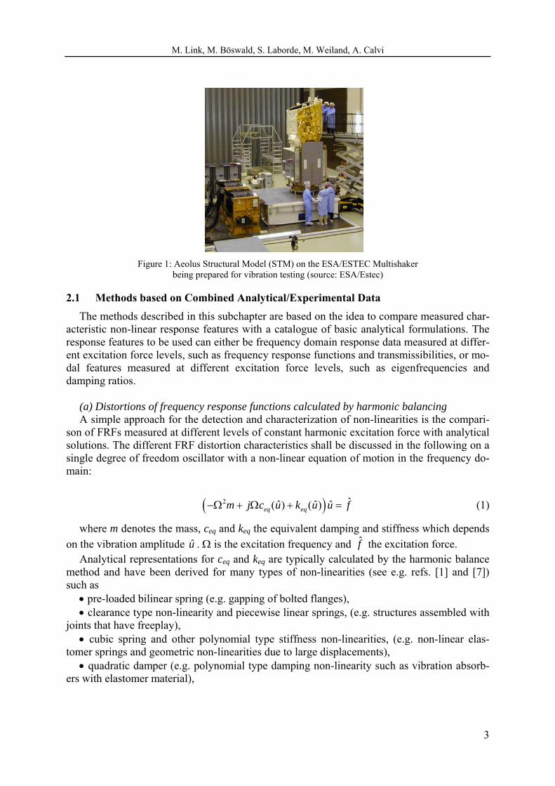
In space industry present experimental vibration test evaluation methods are generally based on the assumption of linear structural behaviour. Test procedures to check the linearity assumption are described in the European Space Agency (ESA) standard on modal survey as-sessment (ECSS-E-ST-32-11C see www.ecss.nl for details) and are applied for base driven tests on the shaking table (an application is shown in Figure 1) as well as in modal survey testing. The resonance shifts and FRF peak variations observed in the case of non-linear struc-tural behaviour are generally not reflected in practice by non-linear analytical modelling. In-stead, equivalent linear modelling adapted to a specified load level is used.

This approach can be tolerated since experience shows that in many practical cases the non-linear structural behaviour is not too strong so that the experimental modal data still lie within the natural scatter generated by other sources of test data variability like fabrication tolerances, multiple assembly or test reproducibility.

When evaluating test data obtained from spacecraft (S/C) qualification testing on a shaking table it is an important goal to characterise the non-linear behaviour of the structure with re-spect to its magnitude (weak or strong) to enable a decision if equivalent linear modelling is applicable or not. Examples of techniques for detection, characterisation and identification of structural non- linearities are described in this paper.

Since existing codes for experimental modal analysis (EMA) rely on the linearity assump-tion, the scatter of the modal identification results when applying such codes to non-linear vi-bration test data will be particularly high. It was therefore one of the goals of a research project realized by a consortium of European space industry and universities associated around EADS ASTRIUM and funded by the European Space Agency (ESA) to identify non-linear modal parameters in addition to the traditional modal parameters related to the underly-ing linear system. The method that was developed and presented in this paper is fully based on experimental data and does not need an analytical model of the structure. In addition, the method was required to be compatible with the test procedures typically applied in vibration testing of spacecraft structures. This means, it is based on transmissibilities of at least three different input levels. Other test data is not required for the method.

2 DETECTION OF NON-LINEAR RESPONSE PROPERTIES

A large number of methods are described in the literature directed towards detection and quantification of structural non-linearities (e.g. refs. [1] – [6]). Examples of the most promis-ing and practically relevant methods will be presented here. A first classification of the avail-able methods is based on the type of data to be used by these methods. Methods for characterizing non-linear structural behaviour may be based on:

• combined analytical/experimental data • experimental frequency-domain response data • experimental time-domain response data • dedicated excitation signals


3

Figure 1: Aeolus Structural Model (STM) on the ESA/ESTEC Multishaker

being prepared for vibration testing (source: ESA/Estec)

2.1 Methods based on Combined Analytical/Experimental Data The methods described in this subchapter are based on the idea to compare measured char-

acteristic non-linear response features with a catalogue of basic analytical formulations. The response features to be used can either be frequency domain response data measured at differ-ent excitation force levels, such as frequency response functions and transmissibilities, or mo-dal features measured at different excitation force levels, such as eigenfrequencies and damping ratios.

(a) Distortions of frequency response functions calculated by harmonic balancing A simple approach for the detection and characterization of non-linearities is the compari-

son of FRFs measured at different levels of constant harmonic excitation force with analytical solutions. The different FRF distortion characteristics shall be discussed in the following on a single degree of freedom oscillator with a non-linear equation of motion in the frequency do-main:

( )2 ˆˆ ˆ ˆ( ) ( )eq eqm j c u k u u f−Ω + Ω + = (1)

where m denotes the mass, ceq and keq the equivalent damping and stiffness which depends on the vibration amplitude u . Ω is the excitation frequency and f the excitation force.

Analytical representations for ceq and keq are typically calculated by the harmonic balance method and have been derived for many types of non-linearities (see e.g. refs. [1] and [7]) such as

• pre-loaded bilinear spring (e.g. gapping of bolted flanges), • clearance type non-linearity and piecewise linear springs, (e.g. structures assembled with

joints that have freeplay), • cubic spring and other polynomial type stiffness non-linearities, (e.g. non-linear elas-

tomer springs and geometric non-linearities due to large displacements), • quadratic damper (e.g. polynomial type damping non-linearity such as vibration absorb-

ers with elastomer material),


4

• elasto-slip friction non-linearity such as the 3-parameter Masing model (e.g. structures with loosely assembled bolted joints and rivet joints) or

• combined stiffness and damping non-linearities (e.g. combinations of the aforementioned types of non-linearities).

The equivalent non-linear stiffness of a pre-loaded bilinear spring is characterised by the stiff-ness parameters k1 and k2 and the transition parameter uc shown in Figure 2(a). These parame-ters can be calculated by the harmonic balance method (e.g. [7]) resulting in

1

2 11

ˆ,ˆ( ) 4 ˆ2 sin 2 cos ,

ˆ2

c

eq cc

k u uk u k k uk u u

uπ α α α

π

∀ ≤⎧⎪= − ⎛ ⎞⎨ ⎛ ⎞+ − + − ∀ >⎜ ⎟⎜ ⎟⎪ ⎝ ⎠⎝ ⎠⎩

(2)

with sinˆcu

uα = .

(a) (b)

Figure 2: Force-displacement diagram and equivalent stiffness of a pre-loaded bilinear spring

The evolution of the equivalent stiffness keq according to equation (2) is shown in Figure

2(b) for a particular single- DOF example. It can be observed that eqk equals the underlying linear stiffness 1k until the displacement amplitude u exceeds the stiffness transition point cu . After exceeding the stiffness transition point the equivalent non-linear stiffness changes dra-matically from its underlying linear value and finally converges towards the average stiffness 1

1 22 ( )k k+ for very large displacement amplitudes. The complex response calculated by itera-tively solving equation (1) with the amplitude dependent equivalent non-linear spring accord-ing to equation (2) exhibits characteristic distortions of the frequency response function (FRF),

ˆˆ /h u f= . Analytical FRFs of the non-linear single-DOF oscillator with pre-loaded bilinear spring simulated by using different constant excitation force levels are shown in Figure 3. It can be seen that for low excitation force levels (and hence low vibration amplitudes) the non-linear FRF does not deviate much from the linear one. In fact, the system remains linear as long as the vibration amplitudes remain smaller than the stiffness transition point. The FRF distortions increase with increasing vibration amplitudes. The resonance frequency shift de-

( )11 22 k k+

1kcu

1kcu

2k


5

creases at large vibration levels which can be explained by the convergence behaviour of the equivalent non-linear stiffness:

ˆ( )

ˆ( ) eqeq

k uu

mω = (3)

Figure 3: FRF distortion caused by pre-loaded bilinear spring

(upper stable response branch only)

It should be noted that the equivalent non-linear stiffness of the bilinear spring without pre-load is independent from the response amplitude and equals the average stiffness 1

1 22 ( )k k+ . Even though the force-displacement curve of the pure bilinear spring is definitely non-linear, it would not cause distortions to the fundamental harmonic FRF. Thus, the bilinear spring without pre-load cannot be analyzed with the (single-) harmonic balance method.

The comparison of analytical non-linear FRFs like those of Figure 3 with experimental FRFs represents a useful tool for characterizing the type of non- linearity, especially when analytical non-linear FRFs are available for a set of oscillators with practical types of non-linearities. For the computation of non-linear FRFs, the response amplitude dependent equiva-lent stiffness and damping formulations for many different types of non-linearities like those mentioned above can be found in textbooks, e.g. refs. [1] and [8] and other publications, e.g. [7], and [9] – [12].

(b) Industrial Example: Aero engine at large response amplitudes Within the EU research project CERES (refs. [6], [13]), a subassembly of an aircraft en-

gine has been tested at different constant harmonic excitation force levels using stepped sine excitation. The force levels were sufficiently high to drive the structure into the non-linear regime. Figure 4 shows the experimental set-up. The Finite Element model is shown in Figure 5 together with the global bending mode exhibiting the strongest non-linear behaviour. In this case, the bolted flange joint between the component IMC and the component CCOC was as-


6

sumed to be the source of non-linear behaviour. This bolted flange joint interface is highly loaded when the global bending mode contributes to high response levels. Other bolted flange joints were loaded much less and are therefore not assumed to cause significant non-linear behaviour.

Figure 4: Aero-engine subassembly supported by bungee cords with a shaker attached1

(a) (b)

Figure 5: FE model, Pick-up locations (a) and bending mode (b) of an aero-engine subassembly

From the measured non-linear driving point FRFs in Figure 6(a) it can be observed that the resonance shifts towards lower frequencies with increasing excitation force level. In addition, the peak response is increasing indicating a reduction of damping with respect to the load level. When comparing the measured non-linear FRFs with analytical FRFs of different types of non-linearity one could conclude that the most appropriate type would be the assumption of a pre-loaded (softening) bilinear spring and a quadratic damper, see restoring force diagrams 1 Photo of test set up at MTU, Munich, and Imperial College, London, UK

driving point

IMC CCOC

IMC CCOC

electrodynamic shaker


7

in Figure 7. A number of such non-linear elements were introduced into the FE model between the components IMC and CCOC.

340 342 344 346

−0.2

−0.1

0

0.1

0.2

0.3

Frequency [Hz]

Acc

el. [

m/s

2 ]

Real Part Analytical FRF

linear1 N10 N20 N30 N40 N50 N60 N70 N

340 342 344 346−0.3

−0.2

−0.1

0

0.1

0.2

0.3

0.4

Frequency [Hz]

Acc

el. [

m/s

2 ]

Real Part Experimental FRF

linear1 N10 N20 N30 N40 N50 N60 N70 N

340 342 344 3460

0.1

0.2

0.3

0.4

0.5

0.6

Frequency [Hz]

Acc

el. [

m/s

2 ]

Imaginary Part Analytical FRF

linear1 N10 N20 N30 N40 N50 N60 N70 N

340 342 344 3460

0.1

0.2

0.3

0.4

0.5

0.6

0.7

Frequency [Hz]

Acc

el. [

m/s

2 ]

Imaginary Part Experimental FRF

linear1 N10 N20 N30 N40 N50 N60 N70 N

(a) (b)

Figure 6: Comparison of analytical (a) and experimental (b) non-linear FRFs

Figure 7: Restoring force functions of non-linear elements used to model the joint non-linearity

From the comparison of the analytical results in Figure 6(b) obtained from computational updating of the non-linear flange joint parameters k1 , k2 , uc and cnl with the experimental re-sults in Figure 6(a) one may conclude that the characteristics and the magnitude of the ana-lytical response is well reflected. See ref. [6] for details of the procedure for numerical parameter updating.

Rf

ucu1k

2k Rf

u

( )1

2 1

,,

cR

c c c

k u u uf

k u u k u u u≤⎧

= ⎨ − + >⎩

, ,

,

,

, 0

, 0

R R nl R lin

R lin lin lin

R nl nl nl

f f ff c u c

f c u u c

= +

= >

= <

,R nlf ,R linf


8

2.2 Methods Based on Experimental Frequency-Domain Response Data

One way to characterise the non-linear behaviour of a structure is the application of differ-ent kinds of signal processing and visualisation tools to the measured frequency response functions. The comparison of the processed data to a certain reference indicates possible de-viations from linear behaviour. Most of the techniques, however, only provide the possibility for detection but not for quantification of non-linear behaviour.

The following methods are widely used for non- linearity detection • Overlay of FRF plots • Frequency isochrones in Nyquist plots • Hilbert transformation of measured FRFs • Inverse FRF plots • Carpet plots of modal damping • Analysis of coherence functions Many examples are reported in the literature for the application of these techniques, e.g.

refs. [2], [4] and [14]. The most simple and most appropriate for practical industrial applica-tions is the analysis of experimental FRF plots measured under different load levels. Such plots are shown in Figures 15 and 19 for the transmissibility test data2 obtained from shaking table testing of the SWARM satellite. The non- linear behaviour is clearly detected from the peak shifts and the amplitude variations depending on the magnitude of load levels.

In a Nyquist plot the imaginary parts of the FRF are plotted versus the real parts at each measured frequency point. Linear responses appear as (almost) circular curves in the Nyquist plot, whereas non-linearities cause distortions from the circular shape.

When the frequency responses (forced response, not FRF) obtained at different levels of excitation are overlaid in a single Nyquist plot, then the deviation of the frequency isochrones (lines connecting points of equal frequency among a set of different response curves) from straight lines indicate the presence of non-linearity, ref.[11]. This can be observed in Figure 8 where the Nyquist plots with frequency isochrones of a linear and a non-linear system are shown. Examples for the other methods mentioned above are described in refs. [1], [2] and [14].

Figure 8: Nyquist plots with frequency isochrones of linear and non-linear system

2 the transmissibility is calculated from the response divided by the table acceleration which is equivalent to the FRF where the response is divided by the excitation force


9

2.3 Methods Based on Experimental Time-Domain Response Data

Time domain methods for the detection and characterization of non-linearities have sig-nificant advantages over frequency-domain methods. The most obvious point is the typical low sampling rate when acquiring frequency domain data. Usually, Shannon’s Theorem is applied, which states that at least two data samples per period of vibration must be acquired to avoid error in subsequent Fourier transformation. It is known, however, that non-linear effects can cause higher harmonic responses. These higher harmonic responses can easily be meas-ured in the time domain by using a sampling rate which can be set 5 or even 10 times higher than for typical FRF measurements. Thus, more information is available from high frequency responses and this can be used to characterize or even identify the non-linearities.

An accepted time-domain approach for the characterization of non-linearities is the restor-ing force surface method according to [15], which has later been published as force-state map-ping according to [16].

The restoring force methods are based on the non-linear equation of motion of a single de-gree of freedom system:

( , , )

( ) ( ) ( ) ( ) ( ) ( ) ( ) ( , , ) ( )R

R

f u u t

mu t d u u t k u u t f t m u t f u u t f t+ + = → + = (4)

( , , ) ( ) ( )Rf u u t f t mu t→ = − (5)

Here, m is the mass of the system, ( )u t is the acceleration response, ( )f t is the time his-

tory of the excitation force. If these quantities are known by measurements, the restoring force ( , , )Rf u u t can be calculated as a function of time. It is obvious from the above equations, that

in case of a linear system, the restoring force is a linear function of displacement ( )u t and also a linear function of velocity ( )u t :

( , , ) ( ) ( )Rf u u t k u t d u t= + (6)

If displacement and velocity response are also available, e.g. from measurements or from

numerical integration of the measured acceleration response, the restoring force can be plotted as a 3D surface over displacement and velocity. In case of a linear system, the restoring force surface is a planar flat surface. The slope of the surface in the displacement direction (i.e. sec-tions of constant velocity but variable displacement) equals the stiffness k . On the other hand, the damping d is the slope of the restoring force surface in the direction of velocity (i.e. sec-tions of constant displacement but variable velocity).

If velocity and displacement response are not available from measurements, they can be derived numerically by integrating the measured acceleration response. Digital filtering and/or offset removal is necessary in this case because otherwise numerical integration can lead to unsatisfactory results.

The utilization of dedicated excitation signals can also be applied for experimental analysis of non-linear structures. For example, when using sinusoidal excitation, the acceleration re-sponse of a non-linear system will be periodic (fundamental harmonic plus a number of


10

higher harmonics). It would be possible to curve-fit the response and to integrate each har-monic individually. This can be done most effectively in the frequency domain.

The three-dimensional restoring force surface produced by the restoring force surface method can be used not only to characterize the type of stiffness and damping non-linearity. By curve-fitting of the 3D surface using a reasonable model for the type of non-linearity, it is possible to identify the coefficients of the non-linear model used. By proceeding this way, a mathematical description for the observed non-linearity can be obtained which is a valuable feedback information for finite element modelling. Based on the identified mathematical model of the non-linearity, it can be assessed up to which response levels an equivalent linear model is sufficient, or respectively, if the non-linearity must be included in the FE model to improve the prediction capabilities in the large response amplitude regime.

As can be seen from equation (6), the restoring force is indeed only a function of the status of the system defined by displacement and velocity. Individual response points of velocity and displacement at each time step will form a repeatable surface provided that the damping non-linearity is not too severe with strong hysteresis character. If this is not the case, the na-ture and shape of the surface will be independent of the time history of the applied force. This, however, requires that a sufficiently large number of independent states are included in the test data for the generation of the restoring force surface. For example, if a pure sinusoidal signal of constant amplitude is used for excitation, only one ellipse in the displace-ment/velocity plane is generated. This is obviously not enough to generate the complete re-storing force surface. In [16] a pure sine excitation with continuously increasing amplitude is used to generate the restoring force surface. In [15], Chebyshev polynomials are used to ex-trapolate the restoring force surface to unmeasured state points.

If the non-linear restoring force is not only a function of the status of the system, i.e. if hys-teresis effects are present in the dynamics of the system under consideration (e.g. systems with elasto-slip type friction non-linearities), the interpretation of the restoring force surface might not be obvious and the method may even fail to produce a repeatable 3D surface.

The simulated response signals of a non-linear single degree of freedom system with a cu-bic hardening spring were analyzed as an example. Due to the relatively low number of inde-pendent states (i.e. independent combinations of displacement and velocity response) in case of sinusoidal excitation, the restoring force surface is not well populated (see Figure 10) even though the harmonic amplitude has been increased linearly. In contrast to sinusoidal excita-tion, random excitation provides a huge number of independent displacement/velocity combi-nations. Consequently, a well populated restoring force surface can be generated (see Figure 9). It must be stated, however, that this is a rather academic statement, because in case of ran-dom excitation, the excitation energy is distributed over a broad frequency range so that very high force RMS values would be required to reach the same response levels compared to harmonic excitation. This can be difficult to achieve with standard laboratory equipment.

In the case of multi- DOF systems selected single modes have to be excited by appropri-ated exciter configurations since the restoring force method is a single- DOF technique. This allows for applying the restoring force method on a single non-linear modal equation of mo-tion. It should be noted that broadband random excitation is not suited for force appropriation. Extensions of the restoring force method to multi DOF systems were developed by Dimitri-adis [17], Wright [18] and Göge [19].


11

Figure 9: Restoring force surface generated from high level random excitation

Figure 10: Restoring force surface generated from sinusoidal excitation

with increasing force amplitude

2.4 Methods Based on Dedicated Excitation Signals One of the best ways of dealing with non-linearities in practical structures is to control the

vibration levels during the measurements. For example, Figure 11(a) shows the frequency re-sponse functions (i.e. upper branch of non-linear FRF) of an analytical single-DOF system with a cubic stiffness non-linearity calculated under harmonic excitation force with different constant excitation force amplitudes. It can be seen that the distortion of the FRFs is increas-ing with increasing force level. As a result, problems can be expected when applying classical (linear) experimental modal analysis to such deformed FRFs. The modal parameters extracted this way will suffer from inaccuracy, especially for the damping and the modal mass due to the distortion of the response curve. Non-linear distortion characteristics of FRFs may lead to additional (artificial) eigenvalues that are difficult to distinguish from true eigenvalues of the system analyzed, see ref. [22]. However, the analysis of FRF distortions can be used for the characterization of the non-linearity, e.g. by comparison with analytical non-linear FRFs of different types of non-linearities as discussed before. Keeping the excitation force level con-stant would mean to increase the level of the drive signal of the electro-dynamic shaker when approaching resonance. This involves an unavoidable risk of damaging the structure in the test, especially in case of lightly damped structures and powerful shakers.

Figure 11(b) shows the calculated FRFs of the same non-linear system now keeping the re-sponse amplitude constant. The legend in Figure 11(b) shows the levels of the constant dis-placement responses of the different simulations. In contrast to Figure 11(a) it can be seen that the excitation force was changed in order to maintain constant response level. By proceeding this way the non-linearity was also kept constant and thus each FRF in Figure 11(b) reflects a


12

linear characteristics (not distorted) with slightly different underlying linear stiffness (in con-trast to Figure 11(a) where all FRFs exhibit non-linear distortions).This approach generates an effectively quasi linear structural behaviour around the main resonances at the different input levels which enables the utilization of classical linear modal extraction tools to be applied separately at each response level. However, the measured dynamic responses (transmissibili-ties) reveal peak shifts and amplitude changes depending on the input level of the base excita-tion which can be utilized to describe the non-linear behaviour.

Another advantage of constant response level testing is that the structure under test can be prevented from being damaged. This requires that the response levels to be investigated have to be defined carefully. It should be mentioned that constant response amplitude levels can only be realized in a narrow frequency band around the resonance of an isolated non-linear mode that is investigated in detail. If broad frequency ranges are considered, many modes may contribute to the response of a structure so that constant response amplitudes can only be realized at a single response DOF. In industrial qualification procedures for spacecraft testing it is common practice to apply input notching in order to avoid overloading of the structure during the qualification test on a shaking table which requires the control of the dynamic re-sponse at specified levels and locations. In this case the table acceleration levels are reduced in the range of the main resonances such that the response of the structure at selected loca-tions does not exceed a specified limit. It could therefore be expected that the responses and load levels around the notching ranges would exhibit similar characteristics like that of Figure 11(b).

This behaviour has been investigated at a typical example taken from a STM satellite struc-ture (Structural Test Model) test campaign. The measured sinusoidal shaking table accelera-tions (input) for three different load levels are shown in Figure 13. The absolute response amplitudes of the 17 largest DOFs around resonance shown in Figure 14 confirm that the goal of constant output control was fulfilled satisfactorily. The corresponding transmissibilities ob-tained from dividing the responses by the table accelerations are shown in Figure 15. The similarity of the curves in Figures 13 and 15 with the curves in Figures 11(b) for the analyti-cal example is obvious. It can be observed that like in Figure 11(b) the transmissibilities in Figure 15 do not exhibit significant distortions so that the utilization of classical linear modal extraction tools may be applied separately for each input level.

3 INTERPOLATION METHOD In the following a technique is described that is aimed at predicting the responses to other

than the measured input levels which is achieved by applying interpolation and extrapolation techniques to the modal data extracted from the transmissibilities measured at three measured input levels, i.e. the experimental data base is formed by three sets of natural frequencies, mode shapes, modal damping values and modal masses related to each load level. The re-sponse prediction at unmeasured load levels is subsequently performed by standard modal synthesis using the inter- or extrapolated modal data.

At least three load levels have to be used for identifying equivalent linear modal data with classical EMA (Experimental Modal Analysis) techniques. This interpolation forms the basis of the ISSPA_NL code which is described in the following. The interpolation starts from clas-sical linear modal analysis data extracted by any existing EMA code (the in-house code ISSPA has been used, ref. [20]) from experimental frequency response functions (FRF) meas-ured at three load levels. Figure 12 shows the principle of the interpolation and extrapolation scheme.


13

(a) constant excitation (b) constant response

Figure 11: FRFs obtained with constant excitation force levels (a) and constant response levels (b)

The three data points for the variable Z on the vertical axis stand for any of the extracted natural frequencies, modal displacements, modal damping values or modal masses. The vari-able A stands for the load level used during the test (e.g. the g-level used on the shaking table). A distinction is made for input levels that lie within the input level range covered by test data (i.e. Aint,i with i=1,2,…) and input levels that lie outside the range covered by test data (i.e. Alow,i and Aup,i). Polynomial interpolation is performed inside the input level range covered by test data, whereas linear extrapolation is applied for input levels that lie outside the range cov-ered by test data. In principle, any suitable polynomial interpolation can be used. However, in the qualification test campaigns of spacecraft structures, three different input levels are typi-cally used, that is a low level, an intermediate level, and the final qualification level. Due to this, the polynomial interpolation cannot go higher than quadratic (parabolic) interpolation in order to maintain compatibility with the spacecraft structures test procedures.


14

Figure 12: Interpolation and extrapolation scheme

It must be stated that the parabolic interpolation of modal parameters lacks physical sig-

nificance. Nonetheless, it is a suitable interpolation between test data points observed at dif-ferent input levels. Therefore, it is clear that the linear extrapolation to input levels outside the input level range covered by test data must be bounded by meaningful limits. In general, the validity bounds of the extrapolation are dependent on the character and strongness of the non-linearity. The validity range of the linear extrapolation are given by Alow ≤ Alow,i ≤ A1 and A3 ≤ Aup,i ≤ Aup where the bounds Alow and Aup have to be specified by the user. Practical limits can be, for example, Alow = 0.9A1 and Aup = 1.1A3.

The parabolic interpolation scheme between levels A1 and A3 is described by

[ ] { }2

1 2 3= + + =

T

i i i iZ a a A a A A a

int, int, int, int (7)

Since this equation must also be valid at the measured load levels A1 to A3 one gets three equations for determining the interpolation constants a1 – a3:

[ ]{ }

2

1 1 1 1

2

2 2 2 2

2

3 3 3 3

1

1

1

= =

⎡ ⎤⎧ ⎫ ⎧ ⎫⎪ ⎪ ⎪ ⎪⎢ ⎥⎨ ⎬ ⎨ ⎬⎢ ⎥⎪ ⎪ ⎪ ⎪⎢ ⎥⎩ ⎭ ⎩ ⎭⎣ ⎦

Z A A a

Z A A a A a

Z A A a

(8)

The vector { }Z holds the measured variables at the three load levels. This equation can eas-

ily be solved for the interpolation constants:

{ } [ ] { }1−=a A Z (9)

Any interior variable iZ int, at any interior load level ,iAint (i=1,2…n) is calculated from

{ } [ ] [ ] { }1

1−= =

⎧ ⎫⎪ ⎪⎨ ⎬⎪ ⎪⎩ ⎭

T

n

Z

Z A A Z

Z

int,

int int

int,

(10a)

A2 A3 Aup,i

Zup,i

Z3 Z2 Zint,i Z1

input level range covered by test data tangent at A1

Z

A1 Alow,i

Zlow,i

tangent at A3

test data interpolated data

Input Level Aint,i


15

where the matrix [ ]TA

int holds the n interior load levels in the form

[ ]

2

1 1

2

1

1

=

⎡ ⎤⎢ ⎥⎢ ⎥⎢ ⎥⎣ ⎦

T

n n

A A

A

A A

int, int,

int

int, int,

(10b)

For the linear extrapolation scheme the tangents of the parabola at load levels A1 and A3 as shown in figure 12 are used which results in the interpolation formula for the lower and the upper range

1 1 1

= + −i i

Z Z Z A A Alow, low,

tan( ( ))( ) (11a)

3 3 3

= + −i i

Z Z Z A A Aup, up,

tan( ( ))( ) (11b)

with 1 2 3 1

2Z A a a Atan( ( )) = + and 3 2 3 3

2Z A a a Atan( ( )) = + where a2 and a3 denote the interpola-tion coefficients of eq.(9).

As stated above, this interpolation and extrapolation scheme can be applied to any modal parameter. In detail, the eigenfrequencies, the damping ratio, the generalized mass, and the elements of the mode shape vectors are interpolated. The new modal parameters interpolated or extrapolated to a new (unmeasured) input level can be used for response synthesis.

4 INDUSTRIAL APPLICATIONS Test data for the first application were measured during a vibration test campaign of a typi-

cal STM satellite structure (Structural Test Model). The shaking table was driven in lateral direction at low, intermediate and qualification g – levels as shown in Figure 13. The data shown in Figure 15 represent the transmissibilities (transfer functions) calculated by division of the sensor responses (at altogether 164 DOFs) by the pilot response which was chosen as the maximum of the four pilot sensors located on the shaking table.

The test data evaluation procedure consisted of the following steps:

(a) Analysis of the transmissibilities over the whole frequency range in order to identify the most significant response areas.

(b) Selection of a frequency range which is considered to be representative for non-linear behaviour. The frequency range around the fundamental resonance in lateral x-direction is presented here which exhibited the most significant peak shifts and large deviations of amplitudes.

(c) Identification of natural frequencies, mode shapes and modal damping values for each load level within the frequency range selected under (b) using ISSPA, ref. [20], classical modal extraction technique.

(d) Extraction of input levels at resonance from pilot response spectra.

(e) Application of ISSPA_NL for prediction of modal data and responses at not meas-ured input levels.


16

Figure 13: Sinusoidal shaking table accelerations (input) low level (black), intermediate (green), qualification level (red)

Figure 14: Nearly constant absolute response amplitudes of the 17 largest DOFs around resonance

(a) Table acceleration (input) notched around resonances

fqual= 13.10 Hz (qualification level), finter= 13.38 Hz (intermediate level), flow= 13.56 Hz (low level) Lqual = 0.0715 g Linter= 0.0350 g Llow= 0.0162 g (b) Table acceleration (pilot sensor) zoomed around first resonances


17

Figure 15: Amplitudes of the 17 largest transmissibilities

Low level (black), intermediate level (green), qualification level (red)

4.1 Identification of Modal Parameters The characteristics of the transmissibilities in Figure 15 permitted the extraction the modal

data separately for each load level using classical curve fitting procedure (ISSPA) which is based on the linearity assumption. The results of experimental modal analysis are summarized in Table 1:

Table 1: Results of linear modal analysis of three different input levels

Input Eigen- Damping

Description Level [g] freq. [Hz] Ratio [%]

Low 0.0162 13.56 0.8

Intermediate 0.0350 13.38 1.3

Qualification 0.0715 13.10 1.7 The following MAC-values compare the mode shapes extracted from the three load levels

(100% would mean perfect agreement): • MAC (low/ intermediate) 93.2 %, • MAC (low/ qualification) 93.0 %, • MAC (intermediate/qualification) 96.9 %.

These numbers and the plot in Figure 17 show

• a small variation of the resonance frequency, • a significant increase of the damping values with the load level, • a small influence of the load level on the mode shapes.

In Figure 16 the good correlation between test and modal synthesis is shown for one repre-

sentative measurement DOF on top of the structure (the correlation for other DOFs was simi-lar). This confirmes the assumption that due to controlled output levels the response of the structure exhibited linear behaviour and that the identified modal parameters are meaningful. Figure 16(a) compares the indicator functions which indicate the quality of modal excitation. In the ideal case when just one single mode contributes to the response the indicator value equals zero. This figure shows that the mode around 13.4 Hz was very well excited. The shift of the resonance frequencies and the variation of the response peaks in Figure 16(b) show the


18

load level dependent nonlinear behaviour equivalent to the analytical system shown in Fig-ure 11(b).

(a) Indicator functions

(b) Transmissibilities

Figure 16: Measured (⎯⎯) and synthesised (• • •) indicator functions (a) and transmissibility amplitudes (b)

low level (black), intermediate level (green), qualification level (red)

4.2 Application of the Interpolation Method The application of the interpolation method seeks to predict the modal data and the re-

sponses at any other than the measured load levels. In the present application two additional load levels were chosen, one at X1add=(Llow+Linter)/2 = 0.0256 g and the other at X2add = (Linter+Lqual)/2 = 0.0532 g, Llow = 0.0162 g, Linter = 0.0350 g and Lqual = 0.0715 g denote the load levels taken at flow = 13.56 Hz, finter = 13.38 Hz and fqual = 13.10 Hz (see Figure 13b).

The basic modal data extracted by the classical (linear) modal extraction technique ISSPA, ref. [20], using the transmissibilities of each load level are used as data points for the interpo-lation functions as described before.

The results of interpolating the modal data between the load levels Llow = 0.0162 g at 13.56 Hz and Lqual = 0.0715 g at 13.10 Hz are shown in Figure 17 (the modal displacements are not shown because of their low variability).

A considerable variation of the modal damping was observed whereas the maximum varia-tion of the resonance frequency is restricted to not more than about 0.5 Hz. Using the modal data at the additional load levels X1add = 0.0256 g and X2add = 0.0532 g together with the mo-


19

dal data from the measured load levels yields the indicator functions and the transmissibilities shown in Figure 18.

It may be noted that the indicator functions and the transmissibilities at the additional load levels exhibit a physically meaningful interpolation between the measured levels and thus seems to confirm the achievement of the goals of the interpolation technique implemented in ISSPA_NL. It should also be noted that the calculation of the load level dependent modal data was based on experimental modal data only, i.e. there was no mathematical model involved.

Figure 17: Resonance frequency and modal damping vs. load level [g]

Figure 18: Indicator functions and transmissibilities using the modal data at two additional load levels (blue) together with the modal data from the measured load levels

(qualification level red, intermediate level green, low level black) From the viewpoint of verifying the predictions it was a disadvantage that the additional

load level were not measured during the test campaign. Therefore, the technique was applied to the data available from the SWARM [21] qualification test campaign where one additional intermediate load level was measured. Figure 19 shows the measured transmissibilities at all

Predicted re-sponse at 2 addi-tional load levels


20

181 test DOFs which exhibit the peak shifts and the amplitude variations depending on the magnitude of load levels.

Figure 19: Measured transmissibilities at all 181 test DOFs

The success of constant output control can again be assessed from the 15 largest responses

plotted in Figure 20. This plot shows that the requirement of constant responses within the notch range was not fulfilled as good as with the data of the previous application in Figure 14. Nonetheless, the described procedure was applied.

Figure 20: Absolute response amplitudes of the 15 largest DOFs around resonances at 58 Hz

low level (black), intermediate level (green), qualification level (red)

At first the modal data in the narrow frequency range around the resonance at about 58 Hz were extracted by linear experimental modal analysis techniques which subsequently were used for interpolation. The results from linear identification of modal parameters from three

low level

intermediate level 1, only used for verification of prediction !

intermediate level 2

qualification level


21

sets of transmissibilities with x-excitation is summarized in Table 2 and displayed in Figure 21 together with the interpolated data at the additional level. The results of the SWARM lin-ear modal identification shows:

• variation of the resonance frequency between 57 Hz and 58.4 Hz, • significant change of the damping values with the load level, • small influence of the load level on the mode shapes (not shown here).

Table 2: Results of SWARM linear modal analysis of three different input levels Input Eigen- Damping

Description Level [g] freq. [Hz] Ratio [%]

Low 0.06 57.00 0.7

Intermediate 0.12 58.14 1.3

Qualification 0.21 58.38 0.5 Using the modal data at the additional load level together with the modal data from the

three measured load levels which were used to derive the fix points for the modal data inter-polation yields the synthesized transmissibilities shown in Figure 22.

From the results in Figure 22 a very good correlation of the synthesized and experimental response can be observed, not only at those three measured load levels which were used to derive the fix points for modal data interpolation but in particular at the one additional load level. The results thus seem to confirm the achievement of the research goal.

additional level additional level

Figure 21: Modal data interpolated at one additional load level


22

Figure 22: Measured (⎯) and synthesised (…) transmissibilities for three load levels: low level (black), interme-diate level (green), qualification level (red) and one additional level (sythesized ○-○-○ , measured ⎯⎯ )

5 CONCLUSIONS Many different tools and methods have been described in the literature for characterization

of non-linearities from vibration test data, e.g. in ref. [23]. This paper does not claim to pre-sent a comprehensive list of such methods. Instead, selected methods have been presented which either utilize combined analytical/experimental data or experimental frequency domain response data obtained with controlled input levels or controlled output levels. According to the experience of the authors, application of methods for characterization of non-linear sys-tems is largely dependent on the compatibility with standard test processes and the respective results that these processes can provide. It was therefore one of the objectives of the DYNAMITED project to summarize available tools and finally to set up a process for identi-fication of non-linear systems.

Due to response control at selected sensor locations during a vibration test on a shaking ta-ble it can be observed that the transmissibilities do not exhibit significant non-linear distor-tions so that the utilization of classical linear modal extraction tools may be applied separately for each input level. However, the measured dynamic responses (transmissibilities) reveal peak shifts and amplitude changes depending on the notched input level of the base excitation which can be utilized to describe the non-linear behaviour.

The technique described in the paper utilizes this well established industrial test procedure to analyze the non-linearity based on controlled response at three different table acceleration levels all of them assumed to be constant within the notching frequency ranges. The technique (implemented in the ISSPA_NL code) aimed at predicting the responses to other than the measured input levels which is achieved by applying interpolation and extrapolation tech-niques to the modal data extracted by classical (linear) experimental modal analysis from the transmissibilities measured at three measured input levels.

The procedure was applied using the test data from a STM satellite structure (Structural Test Model) and also from the SWARM satellite test campaign. For each application one characteristic frequency range was selected exhibiting non-linear behaviour around a domi-nant resonance. Subsequently, natural frequencies, mode shapes and modal damping values were extracted for each load level within the selected frequency ranges which subsequently were used for inter- or extrapolation and used for predicting the responses at one ore more unmeasured load levels.

It was found that for the first application the predicted indicator functions and the transmis-sibilities at the two additional (not measured) load levels exhibit a physically meaningful in-


23

terpolation between the measured levels. In particular this holds for the response prediction for the second application (SWARM satellite), where an additional second intermediate load level was measured but was only used for verification purposes. The good results from both applications thus seem to confirm the achievement of the research goals.

It could be of interest for future research to investigate how the load dependent modal data could be utilized for the parameter identification of a physical non-linear Finite Element model.

REFERENCES [1] K. Worden, G. Tomlinson: “Nonlinearity in Structural Dynamics – Detection, Identifi-

cation and Modelling”, Institute of Physics Publishing, Bristol, 2001

[2] K. Vanhoenacker, J. Schoukens, J. Swevers, D. Vaes: “Summary and Comparing Over-view of Techniques for the Detection of Non-Linearities”, Proc. of the International Conference on Noise and Vibration Engineering ISMA 2002, Leuven, Belgium, 2002

[3] J. Wong, J.E. Cooper, J.R. Wright: “Detection and Quantification of Structural Non-Linearities”, Proc. of the International Conference on Noise and Vibration Engineering ISMA 2002, Leuven, Belgium, 2002

[4] Göge D., Sinapius M., Füllekrug U. and Link M.: “Detection and Description of Non-linear Phenomena in Experimental Modal Analysis via Linearity Plots”. Int. Journal of Non-linear Mechanics 40, 2005

[5] Ewins D.J.: “Modal Testing: Theory, Practice and Application”, 2nd Ed.. Research Stud-ies Press, Baldock, UK , 2000

[6] Böswald M. and Link M.: “Identification of Non-linear Joint Parameters by Using Fre-quency Response Residuals”. Int. Modal Analysis Conf. IMAC XXIII, 2005

[7] Gelb A. and Van der Velde W.E.: “Multiple-Input Describing Functions and Nonlinear System Design”, McGraw Hill, 1968

[8] Ehrich F. And Abramson H.N.: “Nonlinear Vibration” in “Shock and Vibration Handbook”, 4th Edition, edited by Harris C.M. McGraw-Hill, New York, 1995

[9] Budak E., Özgüven H.N.: “Iterative receptance Method for Determining Harmonic Response of Structures with Symmetrical Non-Linearities”, Mechanical Systems and Signal processing (MSSP), 7(1), 1993

[10] Gaul L. And Nitsche R.: “Dynamics of Structures with Joint Connections” in “Structural Dynamics 2000 – Current Status and Further Directions”, Ewins D.J. and Inman D. Eds., Research Studies Press, England, 2001

[11] Tomlinson G.R. and Lam J.: “Frequency Response Characteristics of Structures with Single and Multiple Clearance –Type Non-Linerity”, J. Of Sound and Vibration, 96(1), 1984

[12] Meyer S. And Link M.: Local Non-linear Softening Behavior: “Modelling Approach and Updating of Linear and Non-Linear Parameters Using Frequency Response Residuals”. Proc. Of the 21st IMAC, Kissimmee,USA, 2003

[13] Link M., Staples B., Böswald M., Boettcher Th. and Göge D.: “Linking Analysis to Test – Parameter Identification and Validation”. Proc. of the Int. Conference on Noise and Vibration Engineering (ISMA2004), University of Leuven, Belgium, 2004


24

[14] Maia N.M.M. and Silva J.M.M. Eds., “Theoretical and Experimental Modal Analysis”, Research Studies Press, England, 2000

[15] Masri S.F. and Caughey T.K.: “A Nonparametric Identification Technique for Nonlin-ear Dynamic Problems”, Journal of Applied Mechanics, Vol. 46, pp. 433-447, 1979

[16] Crawley E.F. and Aubert A.C.: “Identification of Nonlinear Structural Elements by Force-State Mapping”, AIAA Journal, Vol. 24(1), pp. 155-162, 1986

[17] Dimitriadis G.: “Experimental Validation of the Constant Level Method for Identifica-tion of Nonlinear Multi Degree of Freedom Systems”, Proc. of the 14th International Congress on Condition Monitoring and Diagnostic Engineering Management, Manches-ter, UK, 2001

[18] Wright J.R., Platten M.F., Cooper J.E. and M. Sarmast M.: “Identification of Multi-Degree of Freedom Weakly Non-Linear Systems using a Model based in Modal Space”, Proc. of the International Conference on Structural System Identification, Kassel, Ger-many, 2001

[19] Göge D., Sinapius M., Füllekrug U. and M. Link M.: “Detection and Description of Non-Linear Phenomena in Experimental Modal Analysis Via Linearity Plots”, Interna-tional Journal of Non-Linear Mechanics, No. 40, pp. 27-48, 2005

[20] ISSPA User’s Manual: http://www.uni-kassel.de/fb14/leichtbau/downloads/ [21] http://www.esa.int/esaMI/Operations/SEM27Z8L6VE_0.html

[22] Böswald M., Göge D., Füllekrug U., Govers Y.: “A Review of Experimental Modal Analysis Methods with respect to their Applicability to Test Data of Large Aircraft Structures”, Proc. of the International Conference on Noise and Vibration Engineering ISMA 2006, Leuven, Belgium, 2006

[23] Kerschen G., Worden K., Vakakis A., Golinval JC.:“Past, Present and Future of Nonlinear System Identification in Structural Dynamics“, Mechanical Systems and Sig-nal Processing, Vol. 20, Issue 3, April 2006, pp. 505-592

Documents

NON-LINEAR EXPERIMENTAL MODAL ANALYSIS AND …congress.cimne.com/eccomas/proceedings/compdyn2011/compdyn201… · 2DLR, Institute of Aeroelasticity 37073 Göttingen, Germany ... ing