Non‐Linear Dimensionality Reduction

Md. Abedul Haque

CS3750, Fall 2011

Dimensionality Reduction

• Linear Dimensionality Reduction Methods– PCA• Finds a low‐dimensional embedding of the data points

that best preserves their variance as measured in the high‐dimensional input space

– Classical MDS• Finds an embedding that preserves the inter‐point

distances.

• Equivalent to PCA when those distances are Euclidean.

Dimensionality Reduction

• A special class of problem– Low dimensional data lying in a very high

dimensional space

– Manifold learning

Manifolds

• Three examples of manifolds

• All three are two‐dim. data embedded in 3D

– Linear, “S”‐shape, “Swiss roll”

• For all three, we would like to recover:

– That the data is only two‐dimensional

– “Consistent” locations for the data in 2D

Manifolds

(a) (b) (c)

• PCA : works for (a)

• Doesn’t do much good for (b) or (c)

– Linear subspace doesn’t explain it well

• What do we mean by “consistent locations”?

– Preserve local relationships and structure

– One possibility: preserve distances

Preserving Local/Global Relationships

• MDS – produces a linear embedding– Preserved all pairwise distances

(a) (b) (a) (b)

• Nonlinear manifold:– local distances (a) make sense

– but, global distances (b) don’t respect the geometry

Solution

• Methods that preserve local structure– Isomap

– LLE (Locally Linear Embedding)

– Eigenmaps

Nonlinear Approach‐ Isomap

• Classical MDS – uses Euclidean distance

• What we really want:– Distance measurements along manifold(geodesics)

– Find low‐dim reconstruction which also has these geodesic distances

• Isomap: Classical MDS with geodesic distances.

Josh. Tenenbaum, Vin de Silva, John langford 2000

Isomap ‐ Algorithm

• Step 1: Construct Neighborhood graph (G)– Define the graph G over all data points by connecting points

i and j if they are • Closer than є – (є‐Isomap)

• If i is one of the k nearest neighbors of j (k‐isomap)

– Set edge lengths equal to dx(i,j)

Josh. Tenenbaum, Vin de Silva, John langford 2000

• Step 2: Compute Shortest Paths in G– Floyd’s algorithm ( O(n3)) to find DG

• Step 3: Construct d‐dimensional embedding– Apply classical MDS on DG to find d‐dimensional embedding

– Finding eigenvectors (O(n3))

Josh. Tenenbaum, Vin de Silva, John langford 2000

Isomap ‐ Algorithm

Isomap

• Advantages– Non‐linear

– Non‐iterative polynomial time algorithm

– Guarantee of globally optimality• For intrinsically Euclidean manifolds, a guarantee of

asymptotic convergence to the true structure

• the ability to discover manifolds of arbitrary dimensionality

• Disadvantages

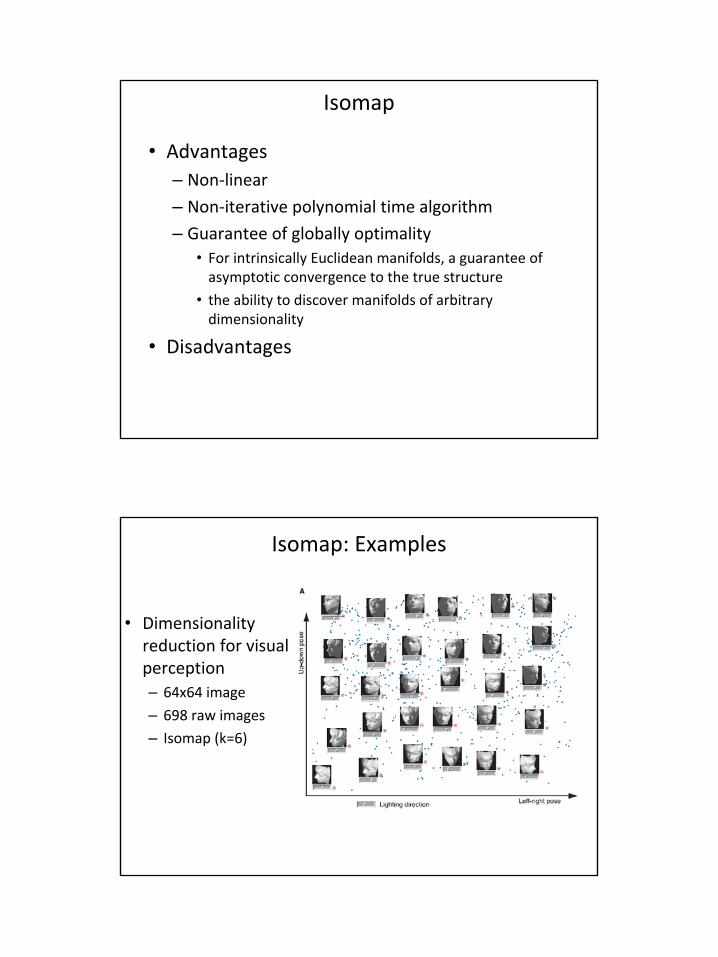
Isomap: Examples

• Dimensionality reduction for visual perception– 64x64 image

– 698 raw images

– Isomap (k=6)

Isomap: Examples

• Handwritten ‘2’– 1000 handwritten 2s

– Isomap (є=4.2)

Isomap: Examples

• Hand images– 64x64 image

– 2000 images

– Isomap (k=6)

Residual Variance

Face ImagesSwisRoll

Hand Images 2

Locally Linear Embedding (LLE)

• Manifold Characteristics/Key Assumption– Provided there is sufficient data, we expect each

data point and its neighbors to lie on or close to a locally linear patch

Sam T. Roweis, L. K. Saul 2000

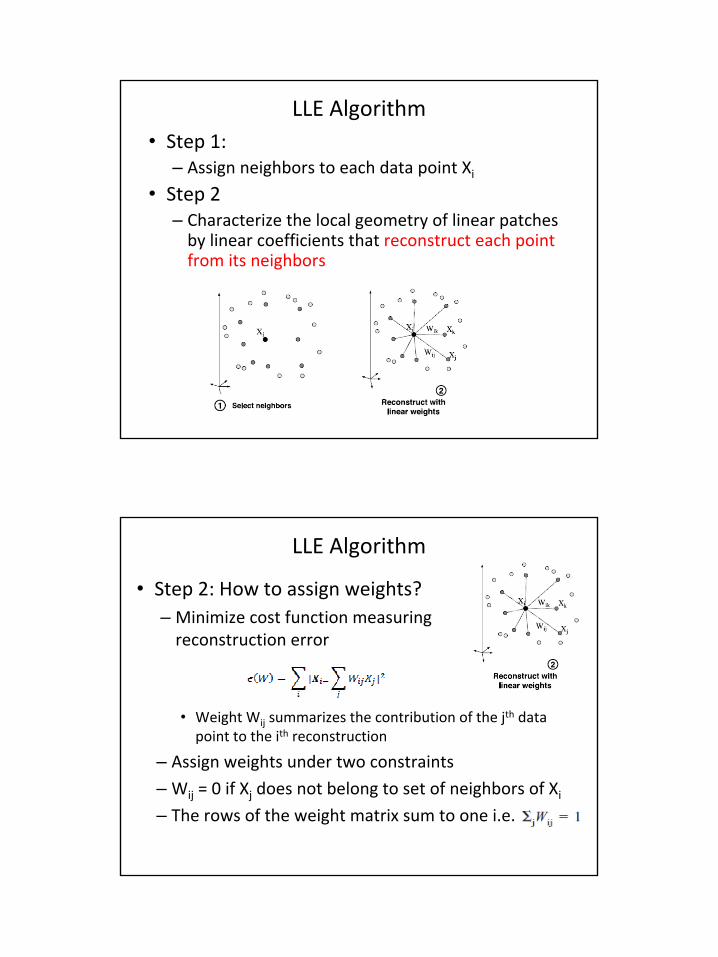
LLE Algorithm• Step 1:– Assign neighbors to each data point Xi

• Step 2– Characterize the local geometry of linear patches

by linear coefficients that reconstruct each point from its neighbors

LLE Algorithm

• Step 2: How to assign weights?– Minimize cost function measuring

reconstruction error

• Weight Wij summarizes the contribution of the jth data point to the ith reconstruction

– Assign weights under two constraints

– Wij = 0 if Xj does not belong to set of neighbors of Xi

– The rows of the weight matrix sum to one i.e.

LLE Algorithm

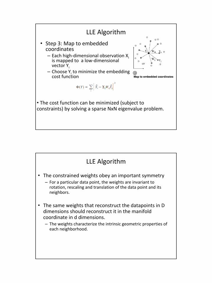
• Step 3: Map to embedded coordinates– Each high‐dimensional observation Xi

is mapped to a low‐dimensional vector Yi

– Choose Yi to minimize the embedding cost function

• The cost function can be minimized (subject to constraints) by solving a sparse NxN eigenvalue problem.

LLE Algorithm

• The constrained weights obey an important symmetry– For a particular data point, the weights are invariant to

rotation, rescaling and translation of the data point and its neighbors.

• The same weights that reconstruct the datapoints in D dimensions should reconstruct it in the manifold coordinate in d dimensions.– The weights characterize the intrinsic geometric properties of

each neighborhood.

LLE Example

Images of faces mapped into the embedding space described by the first two coordinates of LLE. Representative faces are shown next to circled points. The bottom images correspond to points along the top‐right path (linked by solid line) illustrating one particular mode of variability in pose and expression.

Effect of K

• Require dense data points on the manifold for good estimation

Summary: Isomap Vs LLE

• Isomap1. MDS on the geodesic distance matrix2. Global approach3. Requires Dynamic programming

• LLE1. Model local neighborhoods as linear a patches

and then embed in a lower dimensional manifold.2. Local approach3. Computationally efficient. Eigenvectors from

sparse matrices

Laplacian Eigenmaps

• Problem: Given a set (x1, x2, …, xk ) of k points in Rl, find a set of points (y1, y2,…,yk ) in Rm (m << l) such that yi represents xi.

M. Belkin, P. Niyogi 2002

• Steps

– Build the adjacency graph

– Choose the weights for edges in the graph

– Eigen‐decomposition of the graph Laplacian

– Form the low‐dimensional embedding

Laplacian Eigenmaps‐Algorithm

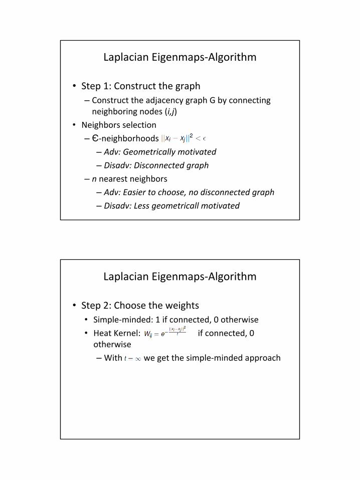
• Step 1: Construct the graph– Construct the adjacency graph G by connecting

neighboring nodes (i,j)

• Neighbors selection

– Є‐neighborhoods

– Adv: Geometrically motivated

– Disadv: Disconnected graph

– n nearest neighbors

– Adv: Easier to choose, no disconnected graph

– Disadv: Less geometricall motivated

Laplacian Eigenmaps‐Algorithm

• Step 2: Choose the weights• Simple‐minded: 1 if connected, 0 otherwise

• Heat Kernel: if connected, 0 otherwise

– With we get the simple‐minded approach

Laplacian Eigenmaps‐Algorithm

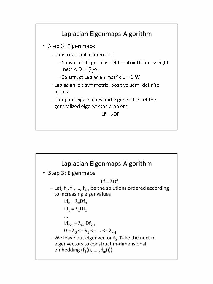
Laplacian Eigenmaps‐Algorithm• Step 3: Eigenmaps

– Let, f0, f1, …, fk‐1 be the solutions ordered according to increasing eigenvalues

Lf0 = λ0Df0

Lf1 = λ1Df1

…Lfk‐1 = λk‐1Dfk‐1

0 = λ0 <= λ1 <= … <= λk‐1

– We leave out eigenvector f0. Take the next m eigenvectors to construct m‐dimensional embedding (f1(i), … , fm(i))

Lf = λDf

Laplacian Eigenmaps‐Justification

• Consider the problem of mapping weighted graph G into a line so that the connected nodes stay as close as possible

• Let y = (y1, y2, … , yn)T be such a map

• Criterion for good map is to minimize ∑ij(yi‐yj)2Wij

Which turns out to be

1/2 ∑ij(yi‐yj)2Wij = yTLy

Laplacian Eigenmaps‐Justification

• Minimization problem

• The constraint removes arbitrary scaling factor• The vector y that minimizes the objective function is

given by minimum eigenvalue solution to the generalized eigenvalue problem

• 1 is an eigenvector corresponding to eigenvalue 0.• To eliminate this trivial solution: Constraint yTD1 = 0

Ly = λDy

Laplacian Eigenmaps‐Justification

• How to find the embedding into m‐dimensional space?

• The embedding is Y = [y1 y2 … ym]

• Objective function:

minimize ∑ij ||y(i) – y(j)||2Wij = tr(YTLY) i.e.

• Solution is provided by the matrix of eigenvectors corresponding to the lowest eigenvalues of the generalized eigenvalue problem

Ly = λDy

Laplacian Eigenmaps

• So each eigenvector is a function from nodes to in a way that "close by" points are assigned "close by" values.

• The eigenvalue of each eigenfunction gives a measure of how "close by" are the values of close by points

• By using the first m eigenfunctions for determining our m‐dimensions we have our solution.

Continuous Manifold

• Laplacian of a graph is analogous to the Laplace Beltrami operator on manifolds.

• Mapping to 1‐D. Find a map f such that points close together on the manifold get mapped close together on the line.

• Two points z and x mapped to f(z) and f(x). It is shown that

Continuous Manifold

• Gradient of f provides us with an estimate of how far apart f maps nearby points.

• Minimizing the gradient minimizes the values assigned to close by points.

• Minimizing the objective function reduces to finding eigenfunctions of the Laplace Beltrami Operator

LLE and Laplacian Eigenmap

• LLE is connected with Laplacian Eigenmap

• LLE minimizes yT(I‐W)T(I‐W)y which reduces to finding eigenvectors of (I‐W)T(I‐W)

• They show that finding eigenvectors of (I‐W)T(I‐W) can be re‐interpreted as finding eigenvectors of iterated Laplacian L2.

Laplacian Eigenmap Example

• Swiss roll

2000 random data points on the manifold

Laplacian Eigenmap Example

• 2D embedding of the swiss roll

Free parameters, N and t. N = Number of neighbors, t = Heat kernel parameter

Laplacian Eigenmap Example• 300 most frequent words from Brown corpus

• Each word is represented by a 600 dimensional vector

• Laplacian Eigenmap with N = 14, t = inf

Framgents labeled by arrows, from left to right. The first is exclusively infinites of verbs, the second contains prepositions and the third mostly modal and auxiliariy verbs

Laplacian Eigenmap Example: Speech

• Speech signal is high dimensional but distinctive phonetic dimensions are few

• 30 ms window at 5 ms interval

• 256 Fourier coefficients for each 30 ms chunk

• 685 such vectors

685 speech data points plotted in the two dimensional Laplacian spectral representation

Laplacian Eigenmap Example: Speech

A blowup of the three selected regions. The data points corresponding to the same region have similar phonetic identity

Summary

• Isomap, LLE and Laplacian Eigenmap: Non‐linear dimensionality reduction technique

• Useful for learning manifolds, understanding low dimensional data embedded in high dimensional space.

• PCA and MDS fails for this type of data.

• All three use some technique to preserve local geometry i.e. inter‐point relationships

References and acknowledgments

• Roweis, S. T. & Saul, L. K. (2000), ‘Locally linear embedding’, Science 290, 2323–2326.

• Tenenbaum, J. B., de Silva, V. & Langford, J. C. (2000), ‘A global geometric framework for nonlinear dimensionality reduction’, Science 290, 2319–2323.

• http://www.cs.nyu.edu/~roweis/lle/• http://isomap.stanford.edu/• http://en.wikipedia.org/wiki/Nonlinear_dimensionality_reduction• http://web.mit.edu/6.454/www/www_fall_2003/ihler/slides.pdf• http://cseweb.ucsd.edu/~saul/teaching/cse291s07/laplacian.pdf• www.public.asu.edu/~jye02/CLASSES/Spring.../Lec19‐Isomap.ppt• www.public.asu.edu/~jye02/CLASSES/Spring.../Lec20‐LLE.ppt• www.public.asu.edu/~jye02/CLASSES/.../Lec21‐LaplacianEig.ppt