Embed Size (px)
Citation preview
NON-CONVENTIONAL ENERGY SOURCES
A PROJECT SUBMITTED IN PARTIAL FULFILLMENT
OF THE REQUIREMENT FOR THE DEGREE OF
Bachelor of Technology
in
Electrical Engineering
By
NAVAL SINGH
Department of Electrical Engineering
National Institute of Technology
Rourkela
2009

NON-CONVENTIONAL ENERGY SOURCES
A PROJECT SUBMITTED IN PARTIAL FULFILLMENT
OF THE REQUIREMENT FOR THE DEGREE OF
Bachelor of Technology
in
Electrical Engineering
By
NAVAL SINGH
Under the guidance of
Prof. SANKARSAN RAUTA
Department of Electrical Engineering
National Institute of Technology
Rourkela
2009
ii
CERTIFICATE OF AUTHENTICITY
This is to certify that the project report titled "Non Conventional Energy Sources" submitted by
Naval Singh, Roll No. 10502067, in fulfillment of the requirements for the final year B. Tech.
project in Electrical Engineering Department of National Institute of Technology, Rourkela is an
authentic work carried out by him under my supervision and guidance.
Date: Prof. Sankarsan Rauta
Dept. of Electrical Engineering
National Institute of Technology
Rourkela- 769008

iii
About the Author
Naval Singh is a Final Year Electrical Engineering student at National Institute of Technology,
Rourkela located at Orissa, an eastern state of India.
When not inside the power electronics laboratory, Naval enjoys spending time with his books,
newspaper and Lenovo Y500 laptop. Naval also draws sketches and paints landscapes (though
seldom simultaneously) and gets into games of badminton and cricket whenever possible.

iv
ACKNOWLEDGEMENT
The thesis of this nature on emerging technologies, such as the wind and photovoltaic power
systems, cannot possibly be written without the help from many sources. I have been extremely
fortunate to receive full support from many individuals in the field. They not only encouraged
me during the project on this timely subject, but also provided valuable suggestions and
comments during the development of the thesis for which I am extremely thankful.
Prof. Bidyadhar Subudhi, head of the Electrical Engineering Department at the NIT Rourkela,
gave me the opportunity to work on the topic and learn new technologies.
Prof. Sankarsan Rauta, my project supervisor, shared with me his long experience in the field.
He helped me develop the project outline for 12 months and gave feedback on my work.
Prof. Saradendu Ghosh, ex-head of Electrical Engineering Department at the NIT Rourkela,
sowed the seeds of simple and cost effective technology development in my mind from early
years at NIT.
Dr. Anup Kumar Panda, Power Electronics Laboratory, NIT Rourkela and Dr. Sharmili Das,
In-charge, Electrical Machines Laboratory, NIT Rourkela, kindly gave me permission to utilize
the resources of their laboratories for my project and provided valuable suggestions for
improvement.
Mr. Rabindra Nayak & Mr. Chhote Laal from PSIM Lab, NIT Rourkela and Mr. Biswanath
Sahoo and Mr. Tirkey from Electrical Machines Lab, NIT Rourkela, provided the much needed
helping hand during my work.

v
I wish to thank my batch-mates who took all my stress away during these months of hard work
with their witty jokes.
Finally this work is dedicated to my mom Mrs. Indu Bala Singh, for the values of discipline,
hardwork and punctuality she instilled in me.
Naval Singh
Roll. No. 10502067
Bachelor of Technology (Electrical Engineering)
NIT Rourkela
Orissa,
India.
E-mail: [email protected], [email protected]
vi
CONTENTS
A Cover page i
B Certificate ii
C About the author iii
D Acknowledgement iv-v
E Contents vi
F Abstract vii
G List of figures viii-xi
H List of tables xii
I Chapters
1: Wind Energy
2: Introduction to solar energy
3: Solar thermal energy conversion systems
4: Solar energy storage
5: Types of solar power plant
6: Gathering Power from Photovoltaic Power Sources
7: Solar photovoltaics
8: PEM Fuel Cell
01-32
33-37
38-41
42-46
47-51
52-108
109-130
131-150
J Conclusion and scope for future work 151
K References 152-155
L Appendix 156-168
Page No.
vii
ABSTRACT
While fossil fuels will be the main fuels for thermal power, there is fear that they will get
exhausted eventually in this century. Therefore other systems based on non-conventional and
renewable sources are being tried by many countries. These are solar, wind, sea, geothermal and
biomass. After making a detailed preliminary analysis of biomass energy, geothermal energy,
ocean thermal energy, tidal energy and wind energy, I focused mainly on Wind power for 7th
semester. In wind power, I have studied mechanical design of various types of wind turbines,
their merits, demerits and applications, isolated and grid-connected wind energy systems with
special attention to power quality. In the end I wrote, compiled and successfully executed a
MATLAB program to assess the impact of a wind farm on the power system.
Solar radiation represents the earth’s most abundant energy source. This energy resource has a
number of characteristics that make it a very desirable option for utilization. The perennial
source of solar energy provides unlimited supply, has no negative impact on the environment, is
distributed everywhere, and is available freely. In India, the annual solar radiation is about 5
kWh/m2 per day; with about 2300-3200 sunshine hours per year.
Solar energy can be exploited for meeting the ever-increasing requirement of energy in our
country. Its suitability for decentralized applications and its environment-friendly nature make it
an attractive option to supplement the energy supply from other sources. In 8th Semester, I have
made an attempt to study the ways through which solar energy can be harnessed and stored. I
have also written MATLAB program to evaluate performance of fuel cell.
viii
List of figures
Chapter Figure Description Page
Number
1 1 Wind turbine 07
2 1 Subsystems in solar thermal energy conversion plants 35
2 Solar Constant 36
5 1 Solar distributed collector power plants 49
2 Solar central receiver power plants 50
3 Central receiver 50
4 Solar pond thermal plant 51
6 1 Solar Cell 55
2 Equivalent circuit of a solar cell 56
3 I-V characteristics of a solar cell 57
4 Elements of SPV system 58
5 Effect of temperature on performance of Silicon solar
module 58
6 I-V characteristics for different insolation levels 59
7 (a) Stand alone PV system, (b) PV –Diesel hybrid system
(c) Grid connected PV system 61
8 No. of battery cycles Vs Depth of Discharge 64
9 Series charge regulators 65
ix
10 Shunt charge regulators 66
11 (a) Buck converter (b) Boost converter (c) Buck-Boost
converter 67
12
(a) I-V characteristics of PV array and two mechanical loads
(b) Speed torque characteristics of DC motor and two
mechanical loads (c) Block diagram for DC motor driven
pumping scheme (d) Block diagram for brushless DC motor
for PV application
70
13 Block diagram for AC motor driven pumping schemes 74
14 Block diagram for V/f control 75
15 Series connection 76
16 Switched PV-Diesel hybrid energy system 79
17 Parallel PV-Diesel hybrid energy system 80
18 Operating modes of PV Diesel hybrid energy system 83
19 Grid interactions (a) VSI (b) CSI 89
20 Line commutated single-phase inverter 90
21 Self commutated inverter with PWM switching 91
22 PV inverter with high frequency transformer 93
23 Half bridge diode-clamped three level inverter 94
24 Non-insulated voltage source 94
25 Non-insulated current source 95
26 Buck converter with half-bridge transformer link 96
27 Flyback Converter 96
x
28 Converter using parallel PV units 97
29 (a) Simple grid interface system (b) Phasor diagram of grid-
integrated PV 98
30 Block diagram of Kalbarri Power Conditioning System 100
31 Central plant inverter 101
32 Multiple string DC/DC converter 102
33 Multiple string inverter 102
34 Module integrated inverter 103
7 1 Hierarchical arrangement of elements of PV system 111
2 Power usage curve 113
3 P-Type Semiconductor 114
4 N-Type Semiconductor 114
5 Schematic of a PV cell 115
- Apparatus Required 121
- Observation: Run 1 122
- Observation: Run 2 122
6 Effect of time on I-V and P-I curve 123
7 V-I and P-I characteristics of SPV module 124
- Cost Analysis 126
8 Experimental Setup 128
Waveform 129
8 1 Schematic of PEFC 134
2 Single cell structure of PEFC 134

xi
3 Plot of Cell Voltage Vs Current Density for different Oxygen
pressure 139
4 Ohmic loss Vs current density 143
5 Ohmic loss Vs fuel cell area 145
6 Water content Vs membrane thickness 147
7 Local conductivity Vs membrane thickness 148
xii
List of tables
Chapter Table No. Description Page No.
6 1 Comparison of different types of motors 71
7 - Calculating savings using PV Walls software 130
Appendix 1 Solar radiation data for New Delhi and Bombay 157
2 Solar radiation & data measurement laboratories in India 158
3 Tabulation of values of ‘a’ and ‘b’ at different locations in India 159
4 Characteristics and features of solar thermal collector systems 160
5 Characteristics of heat transfer fluids 161
6 Reference data of a solar central receiver power plant 162
7 World’s major solar central receiver power plants 163
8 Efficiency of a solar cell 165
Chapter 1
Wind Energy
1
Wind energy
Introduction:
In the continuous search of clean, safe and renewable energy sources, wind power has emerged
as one of the most attractive solutions.
Major factors that have accelerated the wind-power technology development are as follows:
1. high-strength fiber composites for constructing large low-cost blades.
2. falling prices of the power electronics.
3. variable-speed operation of electrical generators to capture maximum energy.
4. improved plant operation, pushing the availability up to 95 percent.
5. economy of scale, as the turbines and plants are getting larger in size.
6. accumulated field experience (the learning curve effect) improving the capacity factor.
India has 9 million square kilometers land area with a population over 1 billion, of which 75
percent live in agrarian rural areas. The total power generating capacity has grown from 1,300
MW in 1950 to about 100,000 MW in 1998 at an annual growth rate of about nine percent. At
this rate, India needs to add 10,000 MW capacity every year. The electricity network reaches
over 500,000 villages and powers 11 million agricultural water-pumping stations. Coal is the
primary source of energy. However, coal mines are concentrated in certain areas, and
transporting coal to other parts of the country is not easy. One-third of the total electricity is used
in the rural areas, where three-fourths of the population lives. The transmission and distribution
loss in the electrical network is relatively high at 25 percent. The environment in a heavily-
2
populated area is more of a concern in India than in other countries. For these reasons, the
distributed power system, such as wind plants near the load centers, are of great interest to the
state-owned electricity boards. The country has adopted aggressive plans for developing these
renewables. As a result, India today has the largest growth rate of the wind capacity and is one of
the largest producers of wind energy in the world.
In 1995, it had 565 MW of wind capacity, and some 1,800 MW additional capacity is in various
stages of planning. The government has identified 77 sites for economically feasible wind-power
generation, with a generating capacity of 4,000 MW of grid-quality power. It is estimated that
India has about 20,000 MW of wind power potential, out of which 1,000 MW has been installed
as of 1997. With this, India now ranks in the first five countries in the world in wind-power
generation, and provides attractive incentives to local and foreign investors. The Tata Energy
Research Institute’s office in Washington, D.C., provides a link between the investors in India
and in the U.S.A.
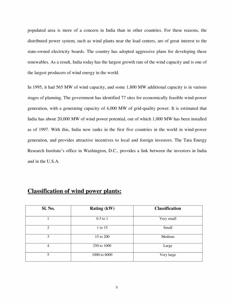
Classification of wind power plants:
Sl. No. Rating (kW) Classification
1 0.5 to 1 Very small
2 1 to 15 Small
3 15 to 200 Medium
4 250 to 1000 Large
5 1000 to 6000 Very large
3
Wind Farms:
1. Wind farms are the areas of land which are mainly used for developing wind power. They have 5 to 50
units.
2. These areas have continuous steady wind speed range of 6 m/s to 30m/s. Annual average wind
speed of 10m/s is considered very suitable.
Wind Energy Density:
Power density of wind is proportional to cube of velocity, i.e. Pw = k. v3= 0.6386. v
3
If A is the swept area of a wind turbine, then P = Pw A
Energy in wind:
Energy is time integral of power.
Energy in ‘n’ hours is given by E = . (Watt-hour)
Area under P-h curve of the wind turbine gives the energy output of the wind turbine.
Efficiency Factor of wind turbine:
Efficiency of the wind turbine is given by the ratio η =
=
4
Power in a wind stream:
A wind stream has total power given by Pt = m. (K.E.w)
= m.Vi
2 (Watt) (1)
where m = mass flow rate of air, kg/s
Vi = incoming wind velocity, m/s
Air mass flow rate is given by
m = ρ A Vi (2)
where ρ = Density of incoming wind, kg/m2 = 1.226 kg/m
2 at 1 atm., 15
0C
A = Cross-sectional area of wind stream, m2
Substituting the value of ‘m’ from (2) into (1), we get
Pt = ρ A Vi
3 (3)
Thus, total power of a wind stream is directly proportional to
1. Density of air , ρ
2. Area of stream, A
3. Cube of velocity, Vi3
Hence the blades of rotor should be long so that the swept area A = π D2/4 is large.
5

Efficiency of a practical propeller type wind turbine:
The maximum efficiency of a propeller type wind turbine is 59%.
Actual efficiency ηa = (0.5 to 0.7) ηmax = 0.6 x 59 = 35.4%
Effect of height on the wind velocity:
In flat, open areas away from cities and forests, the wind speed increases with approximately one seventh
power of the height from ground:
V = H1/7
This relation is valid for the heights between 50m and 250m.
Wind velocity duration curve:
This curve is drawn with number of hours of wind duration per year on X-axis to wind velocity on Y-
axis.
Wind power duration curve:
This characteristic shows “number of hours per year of wind power duration” on X-axis versus
“corresponding wind power” on Y-axis.
Definition of various wind speed for turbines:
1. Cut-in speed: It is speed at which wind turbine starts delivering shaft power.
2. Mean wind speed: Vm = …..
6

3. Rated wind speed: It is the velocity of wind at which the generator produces rated power
output.
4. Cut-out wind velocity (Furling velocity): At high velocities during storms, it is necessary to
cut out the power conversion of wind turbine. The speed at which power conversion is cut out
is called cut-out wind velocity.
Wind turbine:
Wind turbine is a machine which converts wind power into rotary mechanical power. It has
aerofoil blades mounted on rotor.
Figure 1: A wind turbine
7

Wind Turbine Generator units:
A wind turbine generator consists of the following major units:
1. Wind turbine with Horizontal or Vertical axis.
2. Gear chain
3. Electrical generator ( Synchronous or Asynchronous generator )
4. Civil, electrical and mechanical auxiliaries, control panels etc.
Mono-Blade Horizontal Axis Wind Turbine (HAWT):
Features:
1. They have lighter rotor and are cheaper.
2. Blade are 15-25 m long and are made up of metal, glass reinforced plastics, laminated wood,
composite carbon fiber/ fiberglass etc.
3. Power generation is within the range 15 kW to 50 kW and service life of plant is 30 years.
Advantages:
1. Simple and lighter construction.
2. Favorable price
3. Easy to install and maintain.
Disadvantages:
1. Tethering control necessary for higher loads.
8

2. Not suitable for higher power ratings.
Applications:
1. Field irrigation
2. Sea-Water desalination Plants
3. Electric power supply for farms and remote loads.
Twin-Blade HAWT:
1. They have large sizes and power output in range of 1 MW, 2 MW and 3MW.
2. These high power units feed directly to the distribution network.
3-Blade HAWT:
1. 3 blade propeller type wind turbines have been installed in India as well as abroad.
2. The rotor has three blades assembled on a hub. The blade tips have a pitch control of 0 – 30 0
for controlling shaft speed.
3. The shaft is mounted on bearings.
4. The gear chain changes the speed from turbine shaft to generator shaft.
Disadvantages of large HAWT units:
1. Complexity in design involving mechanical, metallurgical & aerodynamic.
2. Extremely high stresses during storms.
3. Installation and repair of large units is difficult.
9
4. Outage affects the power supply to the consumer adversely.
Persian Windmill:
1. The Persian windmill was the earliest windmill installed. ( 7th
Century A.D. – 13th
Century
A.D. in Persia, Afghanistan and China)
2. It is a vertical axis windmill.
3. This windmill was used to grind grains and make flour.
Savonius Rotor:
1. Patented by S.J. Savonius in 1929.
2. It is used to measure wind current.
3. Efficiency is 31%.
4. It is omni-directional and is therefore useful for places where wind changes direction
frequently.
Darrieus Rotor VAWT:
1. It consists of 2 or 3 convex blades with airfoil cross-section.
2. The blades are mounted symmetrically on a vertical shaft.
3. To control speed of rotation mechanical brakes are incorporated. Those brakes consist of steel
discs and spring applied air released calipers for each disc.
10
Wind energy systems:
Based on utilization aspect:
1. Wind electric energy systems connected to grid (without need for energy storage facility).
2. Stand-Alone (Isolated) wind energy systems (with need for energy storage facility).
3. Non-critical wind electric or wind mechanical energy systems (without storage).
4. Wind Electric + Diesel Electric Hybrid or Wind Electric + Solar Electric + Battery hybrid
Based on wind turbine rotor and electrical output:
1. Constant speed constant frequency system
2. Variable speed constant frequency system
3. Nearly constant speed and constant frequency system
Constant speed constant frequency system:
1. Here, shafts of generators are coupled to output shaft of wind turbine. As wind speed is
variable, therefore variable pitch blade control and gears are required to maintain constant
torque output.
2. Constant frequency systems are essential for modern wind farms as the output is either grid
connected or delivered to consumers requiring constant frequency supply.
3. Large WTGs use this method.
Variable Speed Constant Frequency System:
1. Thyristor convertors are used.
2. Due to variable wind speed, the generator produces variable frequency output.
11
3. Rectifier-inverter combination delivers constant frequency electrical output to load or grid.
4. Here, there is no need to regulate blade speed. So, turbine operates at maximum efficiency.
5. Demerit is the additional expense on controls and rectifier-inverter systems.
Nearly constant speed and constant frequency of grid:
1. Small and medium generator units rated 100 kW, 200 kW and 300 kW etc. belong to this
category.
2. They use induction generators and are connected to grid.
3. Excitation current is received from grid. So, induction generator cannot be operated alone.
4. Power factor correction capacitors are also necessary.
Control and monitoring system of a wind farm:
1. A complete wind farm is controlled from the control room located in the main sub-station.
2. (X-1, X-2, X-3 …) represent control cables between individual WTG units and the master
wind turbine controller.
3. The variables like power, voltage, power factor, frequency, rotor speed, pitch angle, bearing
temperature, vibrations, wind direction, wind speed etc. are measured. They are converted to
equivalent digital signals and transmitted via (X-1, X-2 ...) to the master controller.
4. The control has 3 levels:
i) Distribution Network Control Centre
ii) Master Wind Farm Controller
iii) Unit WTG Controller
5. Signals are transmitted by radio signal system.
12

6. Station controller sets the power level according to instructions from the Central Distribution
Control Centre.
Success Stories:
Muppandal–Perungudi (Tamil Nadu)
With an aggregate wind power capacity of 450 MW, the Muppandal–Perungudi region near
Kanyakumari in Tamil Nadu has the distinction of having one of the largest clusters of wind
turbines. About Rs 2500 crores has been invested in wind power in this region.
Kavdya Donger, Supa (Maharashtra)
A wind farm project has been developed at Kavdya Donger at Supa, off the Pune–Ahmednagar
highway, about 100 km from Pune. This wind farm has 57 machines of 1-MW capacity each.
Annual capacity utilization of up to 22% has been reported from this site. The farm is connected
through V-SAT to project developers as well as promoters for online performance monitoring.
Satara district (Maharashtra)
Encouraging policy for private investment in wind power projects has resulted in significant
wind power development in Maharashtra, particularly in the Satara district. Wind power capacity
of about 340 MW has been established at Vankusawade, Thosegarh, and Chalkewadi in Satara
district, with an investment of about Rs 1500 crores.
13

Wind power quality
Power quality is term used to describe how closely the electrical power delivered to customers
corresponds to the appropriate standards so that the equipments of consumers operate
satisfactorily. [Dugan, McGranaghan and Beaty, 1996]
Origin of power quality issues:
1. As load on the generator is removed, wind turbines over-speed. This leads to a high demand
for reactive power which further depresses the network voltage.
2. Network voltage unbalance also affects the rotating induction generators by increasing losses
and introducing torque ripple.
3. Voltage unbalance can also cause power converters to inject unexpected harmonics currents
back into the network.
4. During normal operation, effective rotor resistance to negative sequence currents is very small
Rr/2. So, fault current magnitude is very large.
Electrical behavior of Wind Turbine Generators:
Research conducted by [Heier, 1998], [Fiss, Weck and Weinel, 1993] gives us following
inequality constraints:
For voltage change: ∑ !"(
!#−
!) ≤
For voltage fluctuation: '∑() !"!#
) ≤ *
14
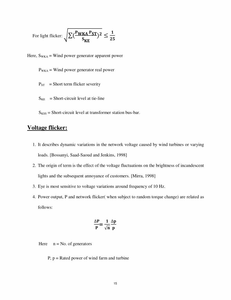
For light flicker: '∑() !" )+!#
) ≤ *
Here, SWKA = Wind power generator apparent power
PWKA = Wind power generator real power
PST = Short term flicker severity
SKE = Short-circuit level at tie-line
SKSS = Short-circuit level at transformer station bus-bar.
Voltage flicker:
1. It describes dynamic variations in the network voltage caused by wind turbines or varying
loads. [Bossanyi, Saad-Saoud and Jenkins, 1998]
2. The origin of term is the effect of the voltage fluctuations on the brightness of incandescent
lights and the subsequent annoyance of customers. [Mirra, 1998]
3. Eye is most sensitive to voltage variations around frequency of 10 Hz.
4. Power output, P and network flicker( when subject to random torque change) are related as
follows:
∆)) =
√.
∆//
Here n = No. of generators
P, p = Rated power of wind farm and turbine
15

∆0, ∆2 = Rated power fluctuation of wind farm and wind turbine respectively.
Harmonics:
1. Thyristors are applied to connect the induction generators to grid. As the firing angle
changes, harmonics are introduced.
2. Therefore anti-parallel Thyristors need to be by-passed during normal operation.
3. Use of IGBTs significantly reduces harmonics of lower order because they operate at kHz
range. High frequency harmonics can be easily filtered.
4. One disadvantage of using IGBTs is that frequencies of kHz range affect the coupling
reactance XC. This causes disturbance in the line models of distribution systems.
16

Comparison of voltage profile of an area before and after the
introduction of a Wind energy plant
(A MATLAB® BASED APPROACH)
Problem Statement:
Output of wind farm is not at constant voltage. Also depending on the operating conditions the
induction generators installed at wind farms absorb or deliver reactive power. This causes
unbalance in the grid to which the wind power plant is connected.
Write a program in MATLAB to compare the effect of voltage profile of an area before and after
the introduction of a Wind energy plant.
Approach:
1. Based on Gauss-Seidel method, a load flow study was formulated.
2. Individual bus admittance values were used to form admittance matrix.
3. Bus 1 was taken as slack bus.
4. Buses 2 & 3 were load buses.
5. Bus 4 was a generator bus connected to a wind farm.
6. Wind farm is an area where a large number of wind mills are installed.
7. The wind farm was considered to have 1000 wind mills.
17
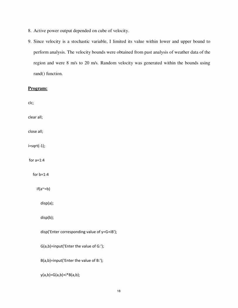
8. Active power output depended on cube of velocity.
9. Since velocity is a stochastic variable, I limited its value within lower and upper bound to
perform analysis. The velocity bounds were obtained from past analysis of weather data of the
region and were 8 m/s to 20 m/s. Random velocity was generated within the bounds using
rand() function.
Program:
clc;
clear all;
close all;
i=sqrt(-1);
for a=1:4
for b=1:4
if(a~=b)
disp(a);
disp(b);
disp('Enter corresponding value of y=G+iB');
G(a,b)=input('Enter the value of G:');
B(a,b)=input('Enter the value of B:');
y(a,b)=G(a,b)+i*B(a,b);
18

end
end
end
% Initialising the Y matrix to zero
for a=1:4
for b=1:4
Y(a,b)=0;
end
end
% % Calculation of Y matrix
for a=1:4
for b=1:4
if(a~=b)
Y(a,b)=-y(a,b);
else
for k=1:4
Y(a,b)=Y(a,b)+y(a,k);
19
end
end
end
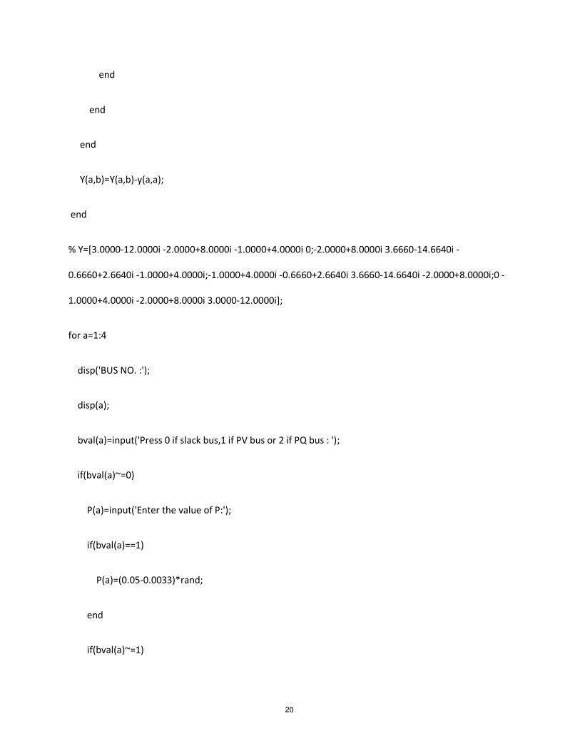
Y(a,b)=Y(a,b)-y(a,a);
end
% Y=[3.0000-12.0000i -2.0000+8.0000i -1.0000+4.0000i 0;-2.0000+8.0000i 3.6660-14.6640i -
0.6660+2.6640i -1.0000+4.0000i;-1.0000+4.0000i -0.6660+2.6640i 3.6660-14.6640i -2.0000+8.0000i;0 -
1.0000+4.0000i -2.0000+8.0000i 3.0000-12.0000i];
for a=1:4
disp('BUS NO. :');
disp(a);
bval(a)=input('Press 0 if slack bus,1 if PV bus or 2 if PQ bus : ');
if(bval(a)~=0)
P(a)=input('Enter the value of P:');
if(bval(a)==1)
P(a)=(0.05-0.0033)*rand;
end
if(bval(a)~=1)
20
Q(a)=input('Enter the value of Q:');
end
end
if(bval(a)>1)
S(a)=-P(a)+i*Q(a);
end
end
% P(2)=0.5;Q(2)=0.2;
% S(2)=-0.5+i*0.2;
% P(3)=0.4;Q(3)=0.3;
% S(3)=-0.4+i*0.3;
% P(4)=(0.05-0.0033)*rand;
reV1=input('Enter Real V1:');
imV1=input('Enter Imaginary V1:');
V1(1)=complex(reV1,imV1);
% V1(1)=1.06+i*0;
21
reV2=input('Enter Real V2:');
imV2=input('Enter Imaginary V2:');
V2(1)=complex(reV2,imV2);
% V2(1)=1+i*0;
reV3=input('Enter Real V3:');
imV3=input('Enter Imaginary V3:');
V3(1)=complex(reV3,imV3);
% V3(1)=1+i*0;
reV4=input('Enter Real V4:');
imV4=input('Enter Imaginary V4:');
V4(1)=complex(reV4,imV4);
% V4(1)=1.04+i*0;
% Assume bus 1=slack, bus 2,3=PQ and bus 4=PV bus
% Calculation of bus voltages
%epsil=input('Enter the value of tolerance:');
22
epsil=0.001;
error=1;
a=2;
Q4up=0.6*0.05/0.8; % Active power (P) generated by wind farm for v=20m/s is 5MW.
Q4low=0.6*0.0033/0.8;% Active power (P) generated by wind farm for v=8m/s is 0.33MW.
while(error>epsil)
R4=real(Y(4,1))*real(V1(1))+real(Y(4,2))*real(V2(a-1))+real(Y(4,3))*real(V3(a-
1))+real(Y(4,4))*real(V4(a-1))-imag(Y(4,1))*imag(V1(1))-imag(Y(4,2))*imag(V2(a-1))-
imag(Y(4,3))*imag(V3(a-1))-imag(Y(4,4))*imag(V4(a-1));
I4=real(Y(4,1))*imag(V1(1))+real(Y(4,2))*imag(V2(a-1))+real(Y(4,3))*imag(V3(a-
1))+real(Y(4,4))*imag(V4(a-1))+imag(Y(4,1))*real(V1(1))+imag(Y(4,2))*real(V2(a-
1))+imag(Y(4,3))*real(V3(a-1))+imag(Y(4,4))*real(V4(a-1));
Q(4)=imag(V2(a-1))*R4-real(V2(a-1))*I4;
if(Q(4)>Q4up)
Q(4)=Q4up;
end
if(Q(4)<Q4low)
Q(4)=Q4low;
end
23
S(4)=P(4)-i*Q(4);
V2(a)=S(2)/conj(V2(a-1));
V2(a)=V2(a)-(Y(2,1)*V1(1)+Y(2,3)*V3(a-1)+Y(2,4)*V4(a-1));
V2(a)=V2(a)/Y(2,2);
abV2(a)=abs(V2(a));
anV2(a)=angle(V2(a));
V3(a)=S(3)/conj(V3(a-1));
V3(a)=V3(a)-(Y(3,1)*V1(1)+Y(3,2)*V2(a)+Y(3,4)*V4(a-1));
V3(a)=V3(a)/Y(3,3);
abV3(a)=abs(V3(a));
anV3(a)=angle(V3(a));
V4(a)=S(4)/conj(V4(a-1));
V4(a)=V4(a)-(Y(4,1)*V1(1)+Y(4,2)*V2(a)+Y(4,3)*V3(a));
V4(a)=V2(a)/Y(4,4);
abV4(a)=abs(V4(a));
24
anV4(a)=angle(V4(a));
err2(a)=abs(V2(a)-V2(a-1));
err3(a)=abs(V3(a)-V3(a-1));
err4(a)=abs(V4(a)-V4(a-1));
errmat=[err2(a) err3(a) err4(a)];
error=max(errmat);
a=a+1;
end
disp('Wind Velocity (wvel)(in m/s):');
wvel=((P(4)*10^8)/638.6)^(1/3)
V2Final=V2(a-1)
V3Final=V3(a-1)
V4Final=V4(a-1)
a
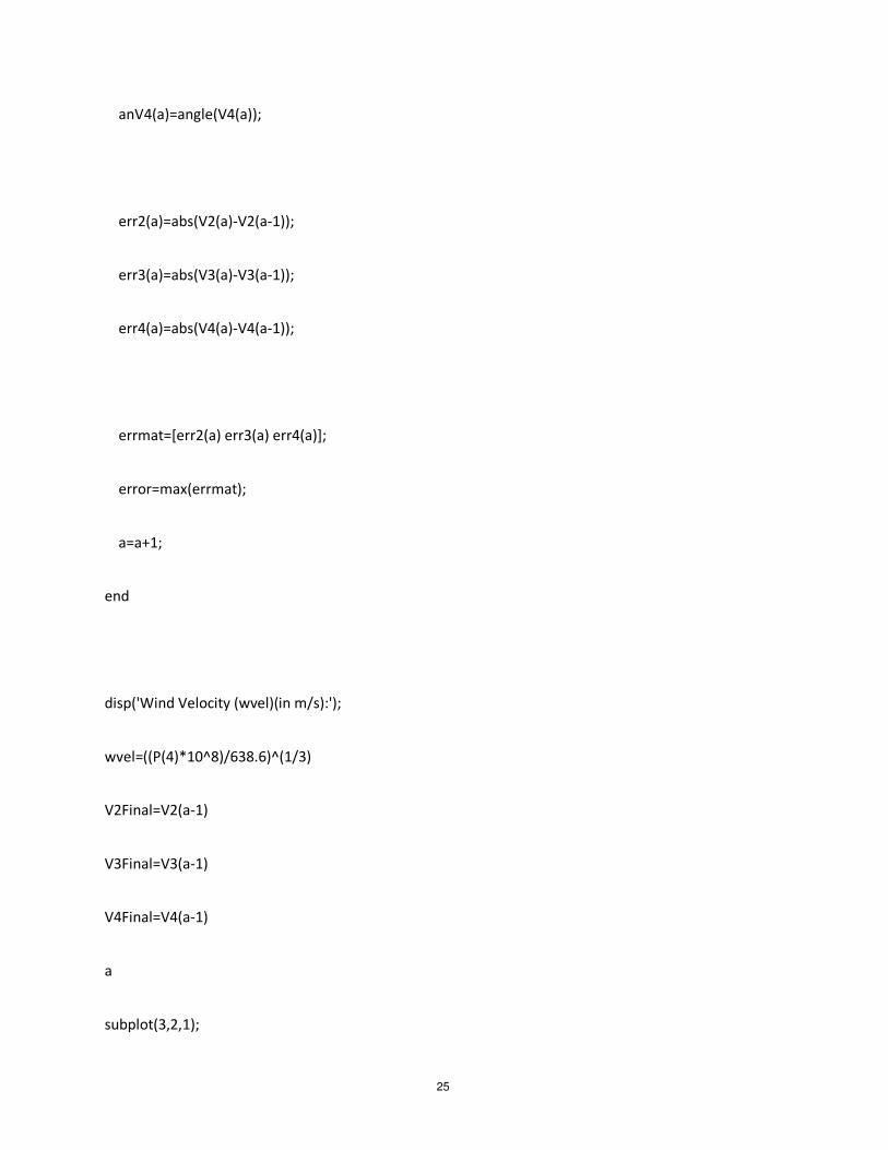
subplot(3,2,1);
25
plot(abV2)
subplot(3,2,2);
plot(anV2)
subplot(3,2,3);
plot(abV3)
subplot(3,2,4);
plot(anV3)
subplot(3,2,5);
plot(abV4)
subplot(3,2,6);
plot(anV4)
% Important Notes:
% There are 1000 wind mills in this Wind Farm. So, output of one wind mill =
% P_one_windmill=P/1000
% P_one_windmill=0.6386*(cube of wind velocity (in m/s))=0.6386*wvel^3
% where P_one_windmill is in Watt.
26
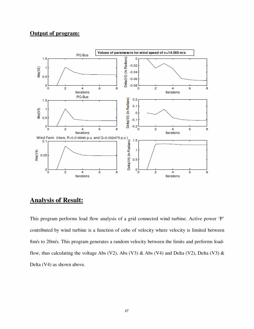
Output of program:
Analysis of Result:
This program performs load flow analysis of a grid connected wind turbine. Active power ‘P’
contributed by wind turbine is a function of cube of velocity where velocity is limited between
8m/s to 20m/s. This program generates a random velocity between the limits and performs load-
flow, thus calculating the voltage Abs (V2), Abs (V3) & Abs (V4) and Delta (V2), Delta (V3) &
Delta (V4) as shown above.
27
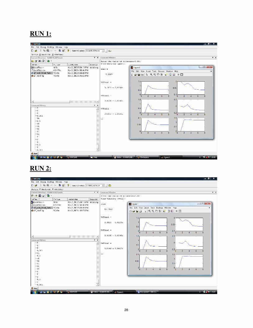
RUN 1:
RUN 2:
28
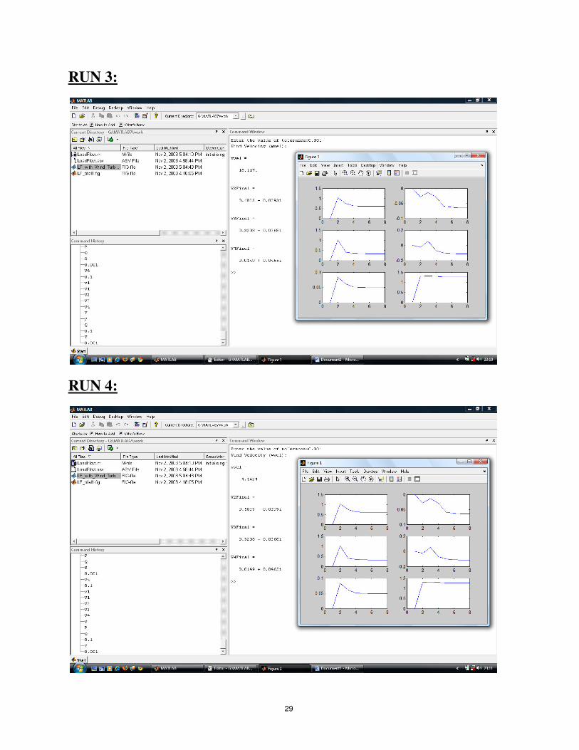
RUN 3:
RUN 4:
29
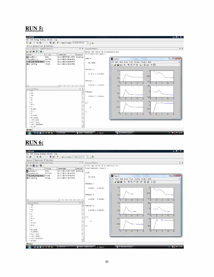
RUN 5:
RUN 6:
30
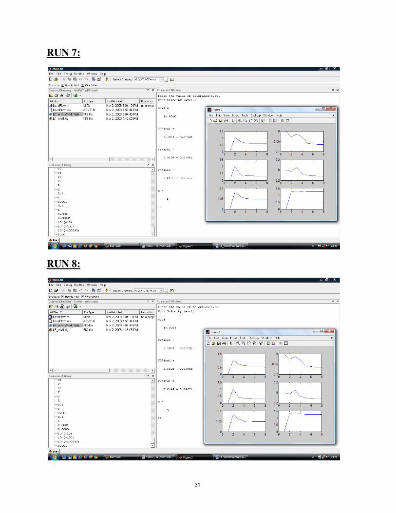
RUN 7:
RUN 8:
31
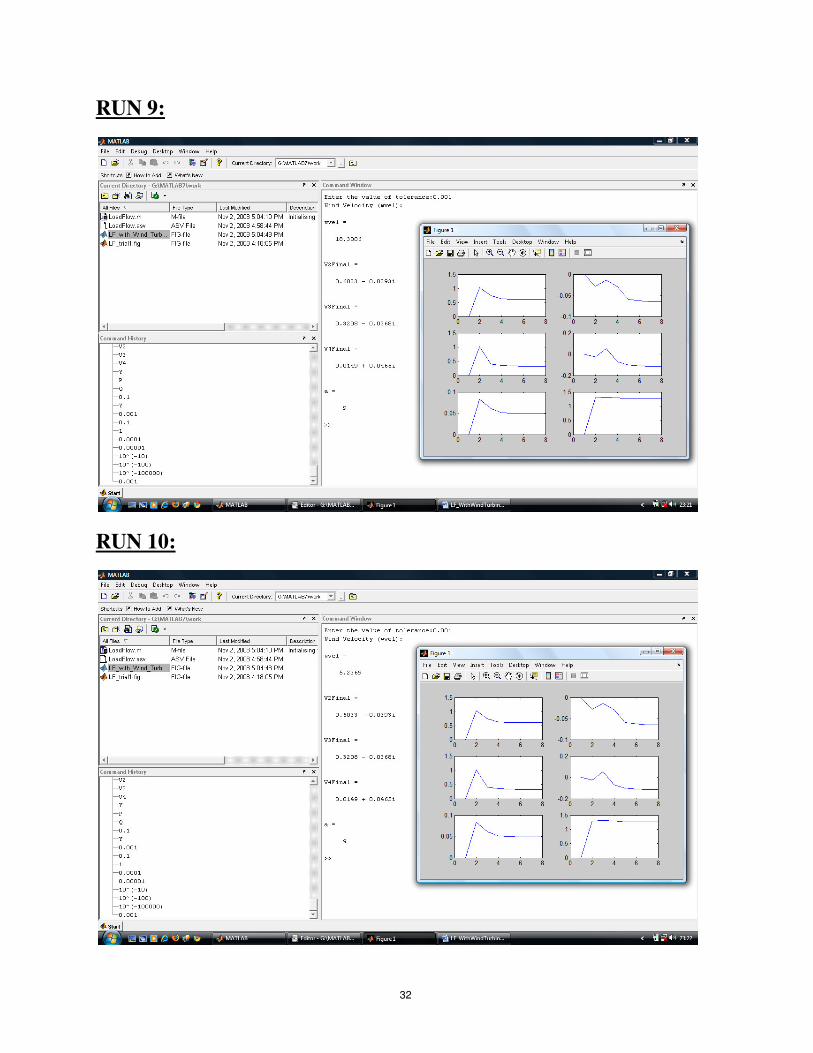
RUN 9:
RUN 10:
32
Chapter 2
Introduction to
solar energy
33
Introduction:
Solar energy is an important, clean, cheap and abundantly available renewable energy. It is received on
Earth in cyclic, intermittent and dilute form with very low power density 0 to 1 kW/m2.Solar energy
received on the ground level is affected by atmospheric clarity, degree of latitude, etc. For design purpose,
the variation of available solar power, the optimum tilt angle of solar flat plate collectors, the location and
orientation of the heliostats should be calculated.
Units of solar power and solar energy: In SI units, energy is expressed in Joule. Other units are angley and Calorie where
1 angley = 1 Cal/cm2.day
1 Cal = 4.186 J
For solar energy calculations, the energy is measured as an hourly or monthly or yearly average and is
expressed in terms of kJ/m2/day or kJ/m
2/hour.
Solar power is expressed in terms of W/m2 or kW/m
2.
Essential subsystems in a solar energy plant: 1. Solar collector or concentrator: It receives solar rays and collects the energy. It may be of following
types:
a) Flat plate type without focusing
b) Parabolic trough type with line focusing
c) Paraboloid dish with central focusing
d) Fresnel lens with centre focusing
e) Heliostats with centre receiver focusing
2. Energy transport medium: Substances such as water/ steam, liquid metal or gas are used to
transport the thermal energy from the collector to the heat exchanger or thermal storage. In solar PV
systems energy transport occurs in electrical form.
3. Energy storage: Solar energy is not available continuously. So we need an energy storage medium
for maintaining power supply during nights or cloudy periods. There are three major types of energy
34
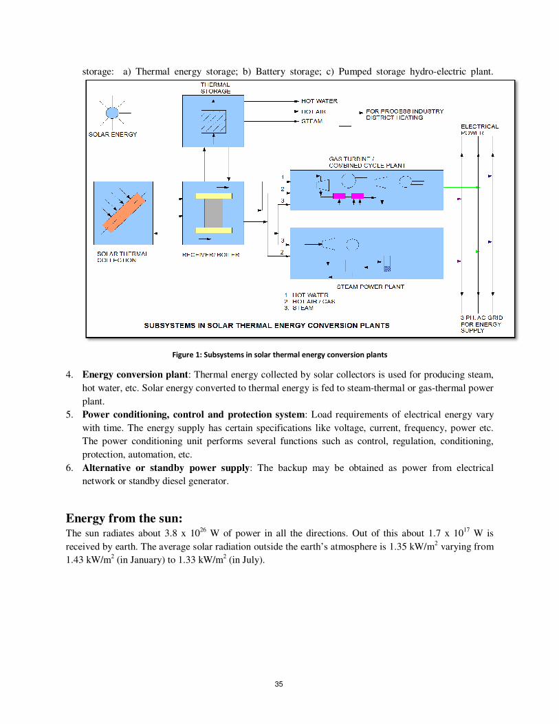
storage: a) Thermal energy storage; b) Battery storage; c) Pumped storage hydro-electric plant.
Figure 1: Subsystems in solar thermal energy conversion plants
4. Energy conversion plant: Thermal energy collected by solar collectors is used for producing steam,
hot water, etc. Solar energy converted to thermal energy is fed to steam-thermal or gas-thermal power
plant.
5. Power conditioning, control and protection system: Load requirements of electrical energy vary
with time. The energy supply has certain specifications like voltage, current, frequency, power etc.
The power conditioning unit performs several functions such as control, regulation, conditioning,
protection, automation, etc.
6. Alternative or standby power supply: The backup may be obtained as power from electrical
network or standby diesel generator.
Energy from the sun: The sun radiates about 3.8 x 10
26 W of power in all the directions. Out of this about 1.7 x 10
17 W is
received by earth. The average solar radiation outside the earth’s atmosphere is 1.35 kW/m2 varying from
1.43 kW/m2 (in January) to 1.33 kW/m
2 (in July).
35
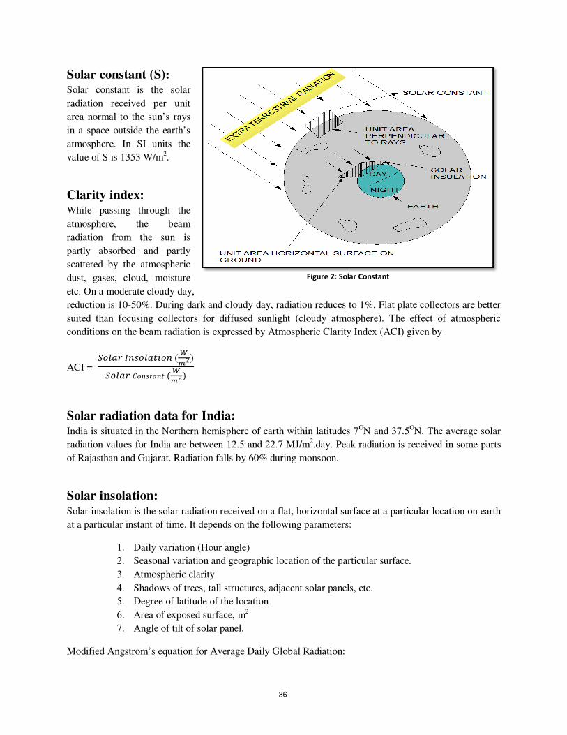
Solar constant (S): Solar constant is the solar
radiation received per unit
area normal to the sun’s rays
in a space outside the earth’s
atmosphere. In SI units the
value of S is 1353 W/m2.
Clarity index: While passing through the
atmosphere, the beam
radiation from the sun is
partly absorbed and partly
scattered by the atmospheric
dust, gases, cloud, moisture
etc. On a moderate cloudy day,
reduction is 10-50%. During dark and cloudy day, radiation reduces to 1%. Flat plate collectors are better
suited than focusing collectors for diffused sunlight (cloudy atmosphere). The effect of atmospheric
conditions on the beam radiation is expressed by Atmospheric Clarity Index (ACI) given by
ACI =
Solar radiation data for India: India is situated in the Northern hemisphere of earth within latitudes 7
ON and 37.5
ON. The average solar
radiation values for India are between 12.5 and 22.7 MJ/m2.day. Peak radiation is received in some parts
of Rajasthan and Gujarat. Radiation falls by 60% during monsoon.
Solar insolation: Solar insolation is the solar radiation received on a flat, horizontal surface at a particular location on earth
at a particular instant of time. It depends on the following parameters:
1. Daily variation (Hour angle)
2. Seasonal variation and geographic location of the particular surface.
3. Atmospheric clarity
4. Shadows of trees, tall structures, adjacent solar panels, etc.
5. Degree of latitude of the location
6. Area of exposed surface, m2
7. Angle of tilt of solar panel.
Modified Angstrom’s equation for Average Daily Global Radiation:
Figure 2: Solar Constant
36
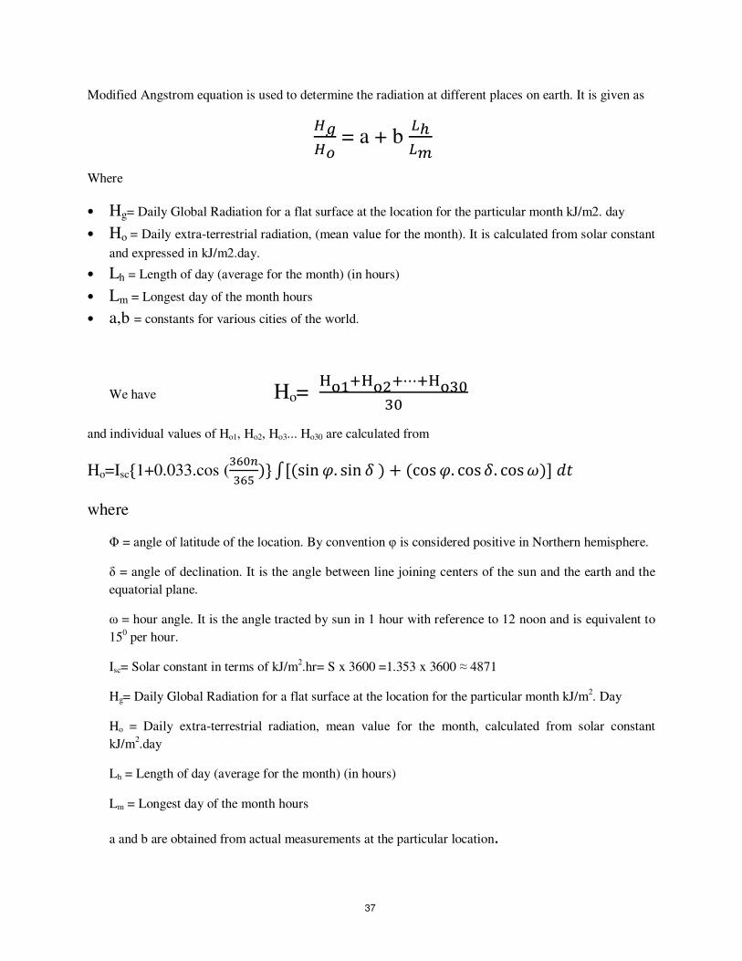
Modified Angstrom equation is used to determine the radiation at different places on earth. It is given as
= a + b
Where
• Hg= Daily Global Radiation for a flat surface at the location for the particular month kJ/m2. day
• Ho = Daily extra-terrestrial radiation, (mean value for the month). It is calculated from solar constant
and expressed in kJ/m2.day.
• Lh = Length of day (average for the month) (in hours)
• Lm = Longest day of the month hours
• a,b = constants for various cities of the world.
We have Ho= HH ⋯H"#
"#
and individual values of Ho1, Ho2, Ho3... Ho30 are calculated from
Ho=Isc1+0.033.cos ("%#
"%& ([sin -. sin / + cos -. cos /. cos3] 5
where
Φ = angle of latitude of the location. By convention φ is considered positive in Northern hemisphere.
δ = angle of declination. It is the angle between line joining centers of the sun and the earth and the
equatorial plane.
ω = hour angle. It is the angle tracted by sun in 1 hour with reference to 12 noon and is equivalent to
150 per hour.
Isc= Solar constant in terms of kJ/m2.hr= S x 3600 =1.353 x 3600 ≈ 4871
Hg= Daily Global Radiation for a flat surface at the location for the particular month kJ/m2. Day
Ho = Daily extra-terrestrial radiation, mean value for the month, calculated from solar constant
kJ/m2.day
Lh = Length of day (average for the month) (in hours)
Lm = Longest day of the month hours
a and b are obtained from actual measurements at the particular location.
37
Chapter 3
Solar thermal energy
conversion systems
38
Introduction:
A solar thermal collector system gathers the heat from the solar radiation and gives it to the heat transport
fluid. The heat-transport fluid receives the heat from the collector and delivers it to the thermal storage
tank, boiler steam generator, heat exchanger etc. Thermal storage system stores heat for a few hours. The
heat is released during cloudy hours and at night. Thermal-electric conversion system receives thermal
energy and drives steam turbine generator or gas turbine generator. The electrical energy is supplied to
the electrical load or to the AC grid. Applications of solar thermal energy systems range from simple solar
cooker of 1 kW rating to complex solar central receiver thermal power plant of 200 MWe rating.
Solar thermal collectors:
As solar power has low density (kW/m2), therefore large area on the ground is covered by collectors. Flat
plate collectors are used for low temperature applications. For achieving higher temperature of transport
fluid, the sun rays must be concentrated and focused.
Concentration Ratio (CR):
CR = (
)
(
)
For flat plate collectors, CR = 1. Using heliostats with sun-tracking in two planes, we obtain CR of the
order of 1000. CR up to 100 can be achieved by using parabolic trough collectors with sun tracking in one
plane.
39
Collector efficiency (η):
The performance of a collector is evaluated in terms of its collector efficiency which is given as
η = ()
()
For constant solar radiation (kW/m2), the collector efficiency decreases with the increasing difference
between the collector temperature and the outside temperature.
Flat plate collector:
Flat plate collector absorbs both beam and diffuse components of radiant energy. The absorber plate is a
specially treated blackened metal surface. Sun rays striking the absorber plate are absorbed causing rise of
temperature of transport fluid. Thermal insulation behind the absorber plate and transparent cover sheets
(glass or plastic) prevent loss of heat to surroundings.
Applications of flat plate collector:
1. Solar water heating systems for residence, hotels, industry.
2. Desalination plant for obtaining drinking water from sea water.
3. Solar cookers for domestic cooking.
4. Drying applications.
5. Residence heating.
Losses in flat plate collector:
1. Shadow effect: Shadows of some of the neighbor panel fall on the surface of the collector where
the angle of elevation of the sun is less than 15O (sun-rise and sunset).
Shadow factor =
40
Shadow factor is less than 0.1 during morning and evening. The effective hours of solar collectors
are between 9AM and 5PM.
2. Cosine loss factor: For maximum power collection, the surface of collector should receive the
sun rays perpendicularly. If the angle between the perpendicular to the collector surface and the
direction of sun rays is θ, then the area of solar beam intercepted by the collector surface is
proportional to cos θ.
3. Reflective loss factor: The collector glass surface and the reflector surface collect dust, dirt,
moisture etc. The reflector surface gets rusted, deformed and loses the shine. Hence, the
efficiency of the collector is reduced significantly with passage of time.
Maintenance of flat plate collector:
1. Daily cleaning
2. Seasonal maintenance (cleaning, touch-up paint)
3. Yearly overhaul (change of seals, cleaning after dismantling)
Parabolic trough collector:
Parabolic trough with line focusing reflecting surface provides concentration ratios from 30 to 50. Hence,
temperature as high as 300OC can be attained. Light is focused on a central line of the parabolic trough.
The pipe located along the centre line absorbs the heat and the working fluid is circulated trough the pipe.
Paraboloid dish collectors:
The beam radiation is reflected by paraboloid dish surface. The point focus is obtained with CR (above
1000) and temperatures around 1000OC.
41
Chapter 4
Solar energy storage
42
Introduction: Unfortunately, the time when solar energy is most available will rarely coincide exactly with the demand
for electrical energy, though both tend to peak during the day light hours. There is also the problem of
clouds with photovoltaic plants, and cloud cover for several days may result in substantially lowered
electrical output compared to high insolation cloud-free days. During such days energy previously stored
during high insolation times could be used to provide a continuous electrical output or thermal output.
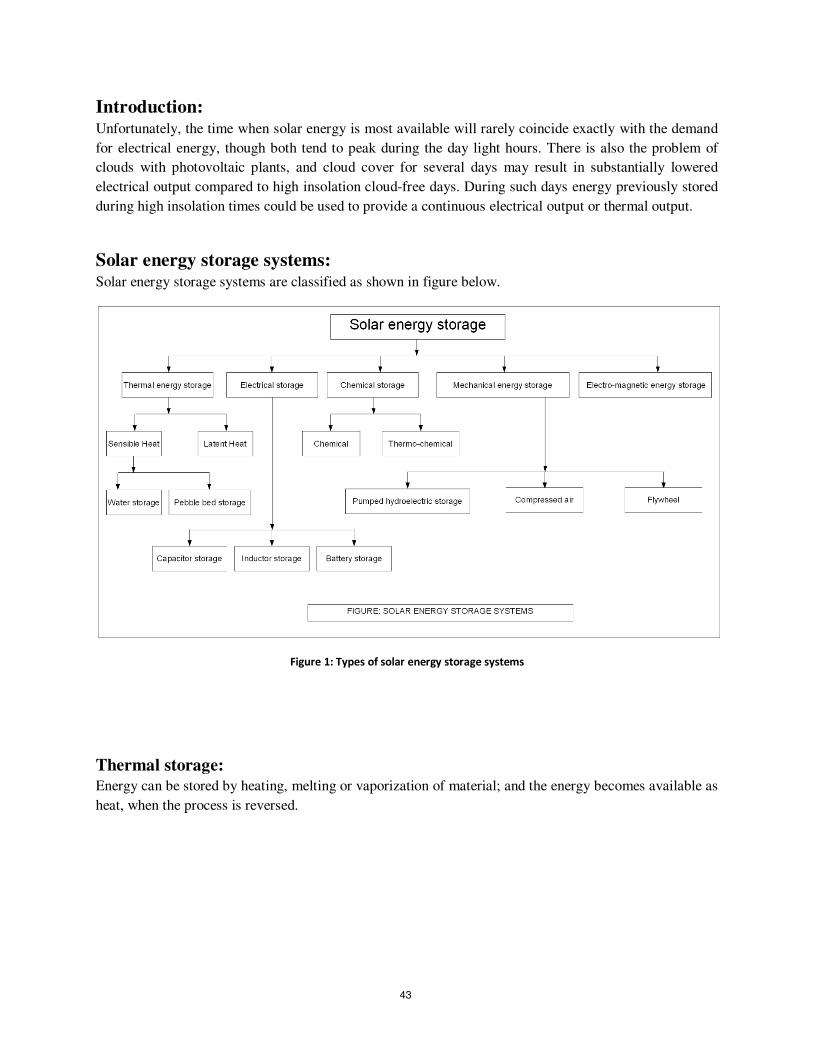
Solar energy storage systems: Solar energy storage systems are classified as shown in figure below.
Figure 1: Types of solar energy storage systems
Thermal storage:
Energy can be stored by heating, melting or vaporization of material; and the energy becomes available as
heat, when the process is reversed.
43
Sensible heat storage: Storage by causing a material to rise in temperature is called sensible heat storage. It involves a material
that undergoes no change in phase. The basic equation for an energy storage unit operating over a finite
temperature difference is
QS = (m. CP)S(T1-T2) = (m. CP)S ∆T
= ∆T
where ρ is the density of the storage medium.
Water storage: The most common heat transfer fluid for a solar system is water, and the easiest way to store thermal
energy is by storing the water directly in a well insulated tank.
Features of water storage are:
1. It is an inexpensive, readily available and useful material to store sensible heat.
2. It has high thermal storage capacity.
3. Energy addition and removal from this type of storage is done by medium itself, thus eliminating
any temperature drop between transport fluid and storage medium.
4. Pumping cost is small.
Pebble bed storage: Here, rock, gravel or crushed stone in a bin provides a large, cheap heat transfer surface. Rock is more
easily contained than water. It acts as its own heat exchanger, which reduces total system cost. Rock can
be easily used for thermal storage at high temperatures (above 100OC). If water storage is used above
100OC, then pressurized storage is required to contain steam. Hence, pebble bed storage has low cost of
storage material. This type of storage system has been used in the solar houses or with hot air collector
system.
Latent heat storage (Phase change energy storage): Here, heat is stored in a material when it melts and extracted from the material when it freezes. Glauber’s
salt (Na2SO4.10H2O) changes phase from solid to liquid requires lesser energy than those from liquid to
gas. It decomposes at about 32OC releasing 56kCal/kg.
44
Electrical storage: 1. Energy stored in capacitor is given as
H=
2
Where V = volume of dielectric
E = electric field strength
Electric field strength is limited by the breakdown strength (Ebr) of the dielectric (e.g. mica).
As the conductivity of dielectric is finite, therefore losses occur in the storage battery.
2. Inductors store energy at low voltage and high current. The energy is given by
H=
2
Where µ = permeability of material
Hm = magnetic flux density
For H to be large, both µ and Hm should be large. Higher magnetic fields exert large forces on structure.
So the structure must be mechanically strong.
3. Battery storage:
1. Energy efficiency (η) of battery storage is given as
η =
Where I1= battery discharge current
E1=battery discharge terminal voltage
I2 = battery charging current
E2= battery charging terminal voltage
t1 = battery discharging time
t2 = battery discharging time
2. Cycle life of battery storage is the number of times the battery can be charged and discharged
under specified conditions.
45
Chemical storage: Solar energy can be stored chemically in the form of fuel. The battery is charged photo-chemically and
discharged electrically whenever needed. It is also possible to electrolyze water with solar electricity
generated, store H2and O2 and recombine in a fuel cell to regain electrical energy. Solar energy can be
converted into methane by anaerobic fermentation of algae. 1km2 of algae field can produce methane
carrying 4MW of solar energy.
Thermo-chemical energy storage (Reversible): Thermo-chemical energy storage systems are suitable for medium or high temperature applications only.
Their major advantage is high energy density at ambient temperatures for long periods without thermal
losses.
Pumped hydroelectric storage of solar energy: Electric power in excess of the immediate demand is used to pump water from a supply (e.g. like, river or
reservoir) at a lower level to a reservoir at a higher level. When power demand exceeds the supply, the
water is allowed to flow back down through a hydraulic turbine which drives an electric generator.
Efficiency of pumped storage is around 70%.
Compressed air storage: Here, the extra energy is stored in the form of a compressed air volume. When energy demand is high,
this air can be used to drive wind turbine to generate electric power.
Flywheel storage: A flywheel driven by an electric motor during off peak hours stores mechanical energy as it gains speed.
The rotational energy of flywheel is used to drive generator to produce electricity.
46
CHAPTER 5
Solar power plant
47

Introduction: Solar electrical power plants require large collection field covering several km
2 area, complex and costly
sun-tracking system for large heliostats, long piping system and large thermal storage system.
Types of solar power plant: 1. Solar distributed collector power plants
2. Solar central receiver power plants
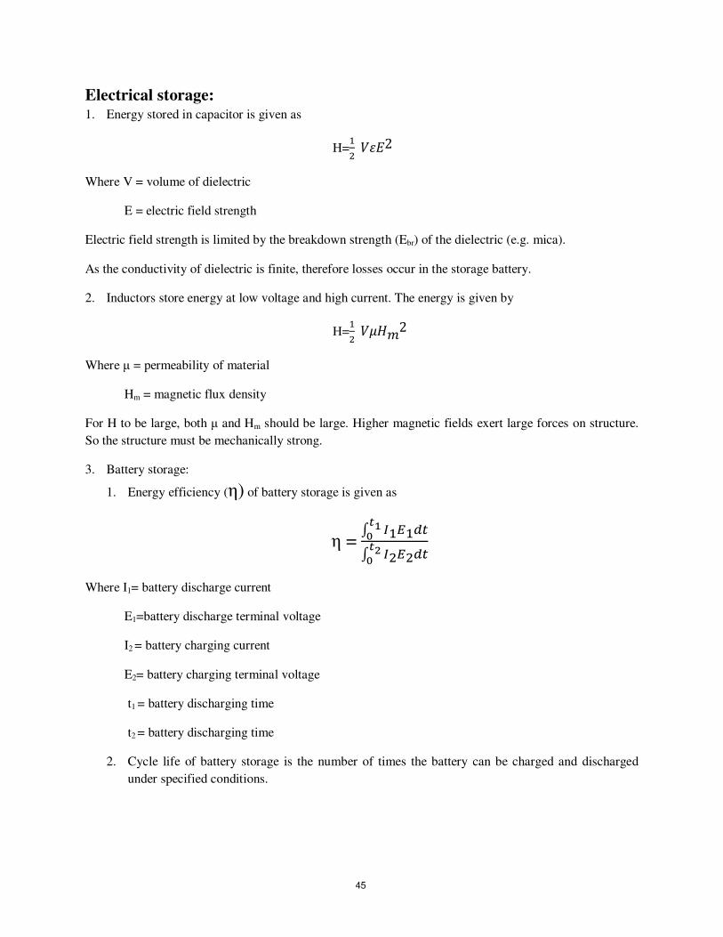
Solar distributed collector power plants: In distributed receiver power plants, parabolic trough collectors with line focus are most commonly used.
The sun rays are reflected by parabolic or cylindrical troughs. The reflected rays are focused on linear
conduit (pipe) located along the axis of the trough.
Figure 1 shows a schematic diagram of a distributed collector solar thermal power plant. The major
components are the following:
1. Trough collectors distributed in the solar field
2. Piping system for primary heat transport loop
3. Heat transport fluid pump
4. Boiler cum steam generator
5. Secondary (working) fluid loop (steam)
6. Steam turbine
7. Turbo-generator
8. Condenser
9. Hot condensate pump – Water loop
10. Feed water heater- Steam loop
11. Boiler feed pump
48
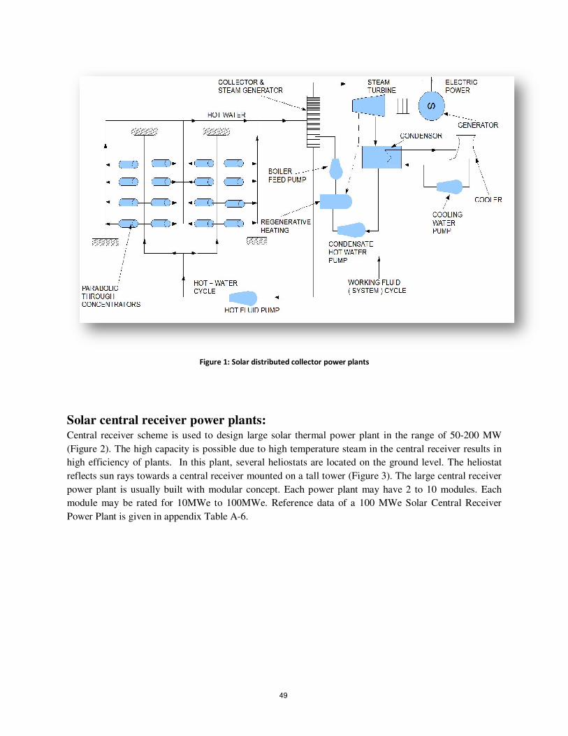
Figure 1: Solar distributed collector power plants
Solar central receiver power plants: Central receiver scheme is used to design large solar thermal power plant in the range of 50-200 MW
(Figure 2). The high capacity is possible due to high temperature steam in the central receiver results in
high efficiency of plants. In this plant, several heliostats are located on the ground level. The heliostat
reflects sun rays towards a central receiver mounted on a tall tower (Figure 3). The large central receiver
power plant is usually built with modular concept. Each power plant may have 2 to 10 modules. Each
module may be rated for 10MWe to 100MWe. Reference data of a 100 MWe Solar Central Receiver
Power Plant is given in appendix Table A-6.
49
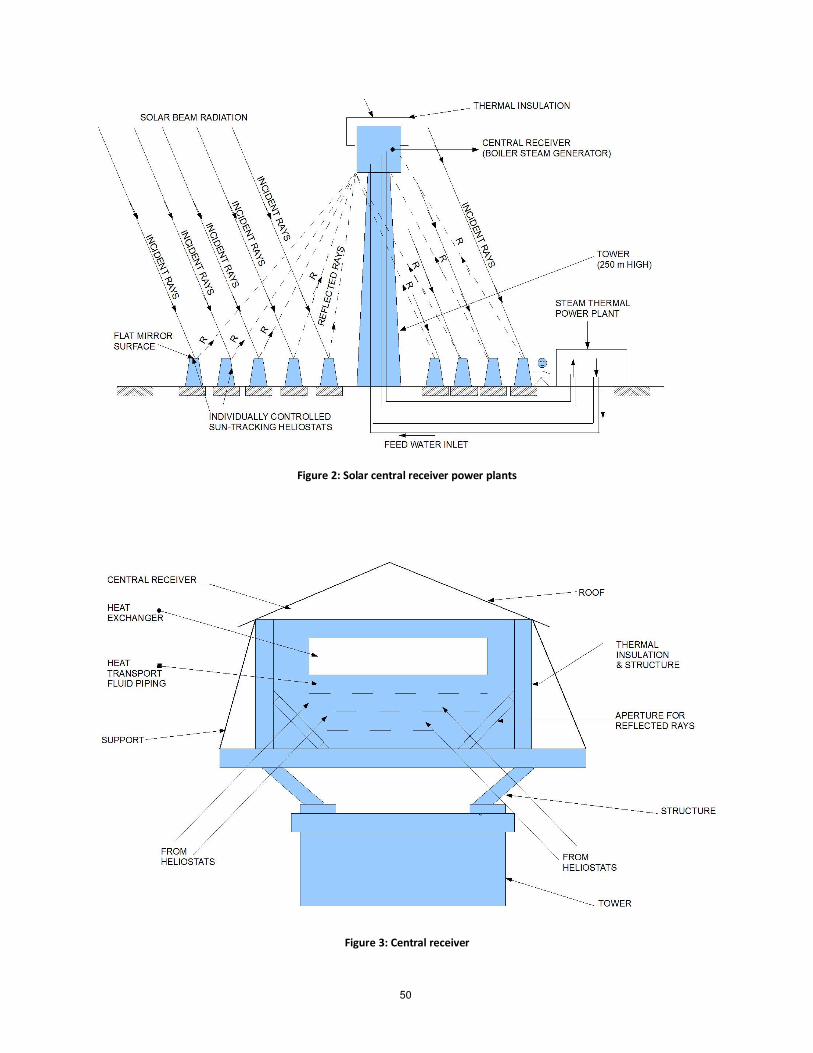
Figure 2: Solar central receiver power plants
Figure 3: Central receiver
50
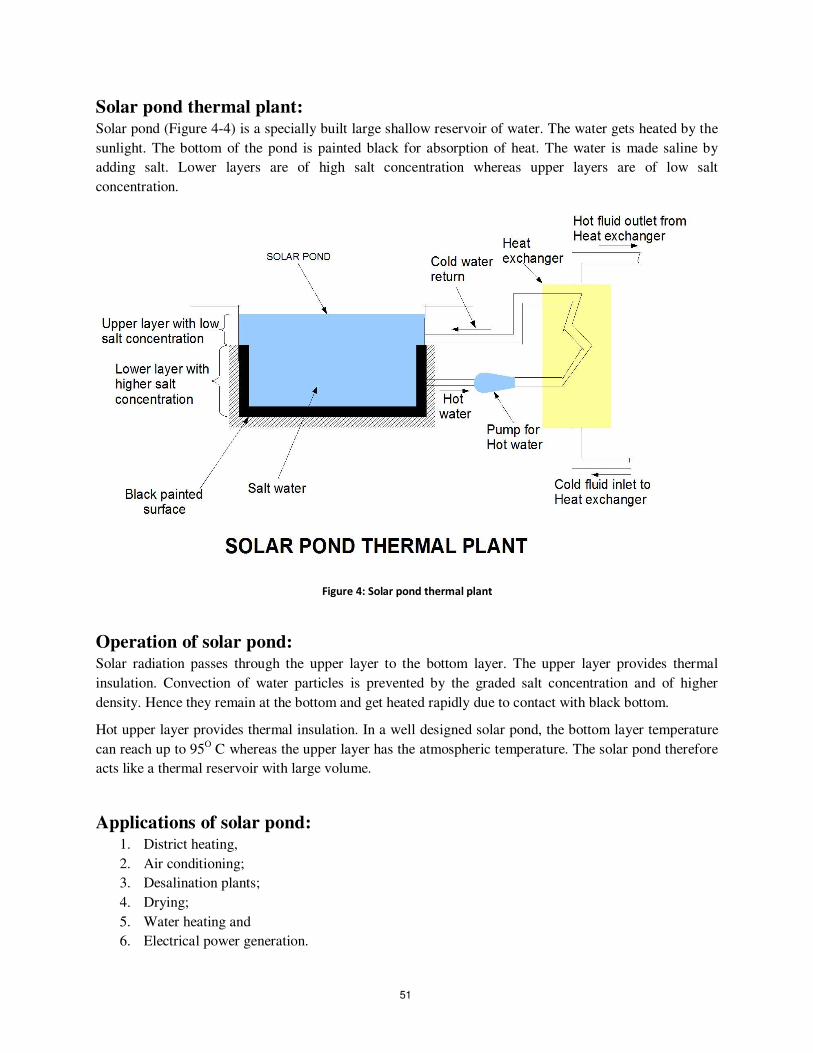
Solar pond thermal plant: Solar pond (Figure 4-4) is a specially built large shallow reservoir of water. The water gets heated by the
sunlight. The bottom of the pond is painted black for absorption of heat. The water is made saline by
adding salt. Lower layers are of high salt concentration whereas upper layers are of low salt
concentration.
Figure 4: Solar pond thermal plant
Operation of solar pond: Solar radiation passes through the upper layer to the bottom layer. The upper layer provides thermal
insulation. Convection of water particles is prevented by the graded salt concentration and of higher
density. Hence they remain at the bottom and get heated rapidly due to contact with black bottom.
Hot upper layer provides thermal insulation. In a well designed solar pond, the bottom layer temperature
can reach up to 95O C whereas the upper layer has the atmospheric temperature. The solar pond therefore
acts like a thermal reservoir with large volume.
Applications of solar pond: 1. District heating,
2. Air conditioning;
3. Desalination plants;
4. Drying;
5. Water heating and
6. Electrical power generation.
51

Chapter 6
Gathering Power from
Photovoltaic Power Sources
52
6.1: Introduction
The Kyoto agreement on global reduction of greenhouse gas emissions has prompted renewed
interest in renewable energy systems worldwide. Many renewable energy technologies today are
well developed, reliable, and cost competitive with the conventional fuel generators. The cost of
renewable energy technologies is on a falling trend and is expected to fall further as demand and
production increases. There are many renewable energy sources such as biomass, solar, wind,
mini-hydro, and tidal power. One of the advantages offered by renewable energy sources is their
potential to provide sustainable electricity in areas not served by the conventional power grid.
The growing market for renewable energy technologies has resulted in a rapid growth in the need
for power electronics. Most of the renewable energy technologies produce DC power, and hence
power electronics and control equipment are required to convert the DC into AC power.
Inverters are used to convert DC to AC. There are two types of inverters: stand-alone and grid-
connected. The two types have several similarities, but are different in terms of control functions.
A stand-alone inverter is used in off-grid applications with battery storage. With backup diesel
generators (such as PV–diesel hybrid power systems), the inverters may have additional control
functions such as operating in parallel with diesel generators and bidirectional operation (battery
charging and inverting). Grid-interactive inverters must follow the voltage and frequency
characteristics of the utility-generated power presented on the distribution line. For both types of
inverters, the conversion efficiency is a very important consideration. Details of stand-alone and
grid-connected inverters for PV and wind applications are discussed in this chapter.
53
Section 6.2.5.2 covers stand-alone PV system applications such as battery charging and water
pumping for remote areas. This section also discusses power electronic converters suitable for
PV–diesel hybrid systems and grid-connected PV for rooftop and large-scale applications.
6.2 Basics of Photovoltaics
The density of power radiated from the sun (referred to as the ‘‘solar energy constant’’) at the
outer atmosphere is 1.373kW/m2. Part of this energy is absorbed and scattered by the earth’s
atmosphere. The final incident sunlight on earth’s surface has a peak density of 1kW/m2 at noon
in the tropics. The technology of photovoltaics (PV) is essentially concerned with the conversion
of this energy into usable electrical form. The basic element of a PV system is the solar cell.
Solar cells can convert the energy of sunlight directly into electricity. Consumer appliances used
to provide services such as lighting, water pumping, refrigeration, telecommunications, and
television can be run from photovoltaic electricity.
Solar cells rely on a quantum-mechanical process known as the ‘‘photovoltaic effect’’ to produce
electricity. A typical solar cell consists of a p n junction formed in a semiconductor material
similar to a diode. Figure 1 shows a schematic diagram of the cross section through a crystalline
solar cell [1]. It consists of a 0.2–0.3mm thick mono-crystalline or polycrystalline silicon wafer
having two layers with different electrical properties formed by ‘‘doping’’ it with other
impurities (e.g., boron and phosphorus). An electric field is established at the junction between
the negatively doped (using phosphorus atoms) and the positively doped (using boron atoms)
silicon layers. If light is incident on the solar cell, the energy from the light (photons) creates free
54
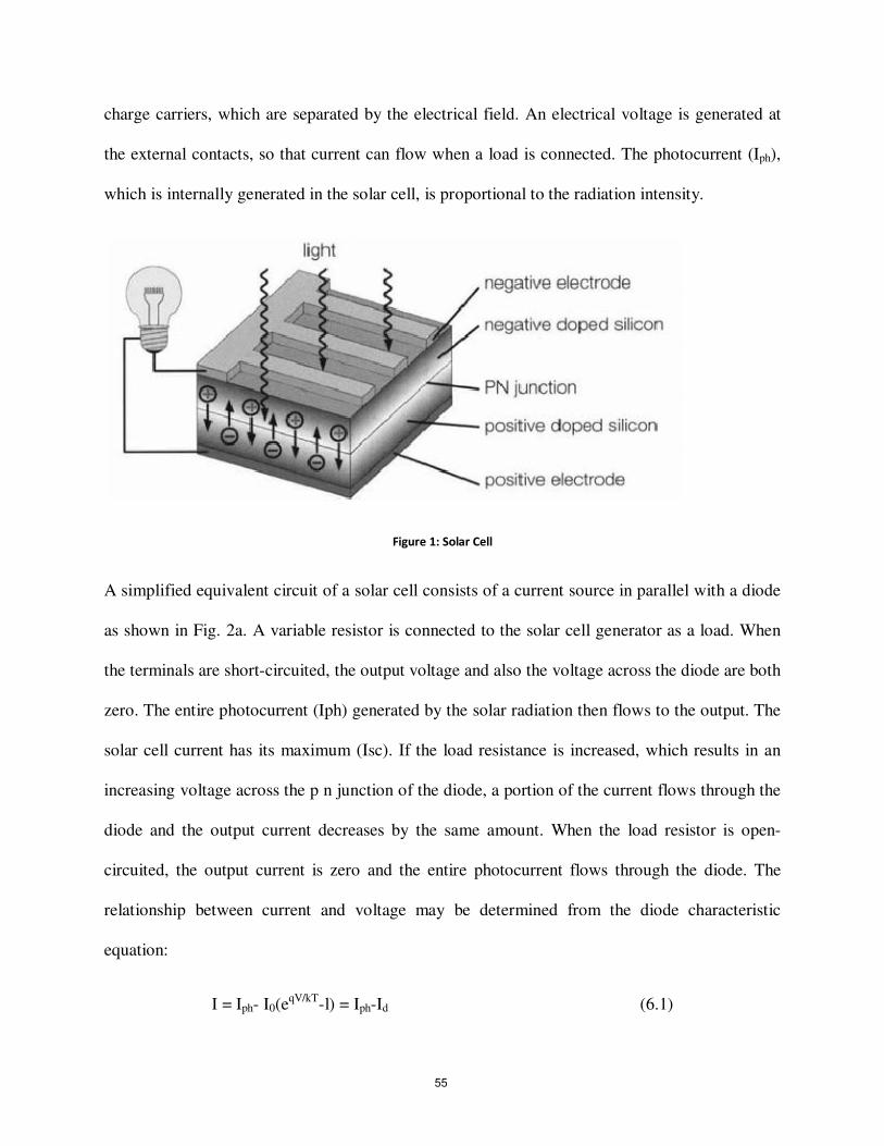
charge carriers, which are separated by the electrical field. An electrical voltage is generated at
the external contacts, so that current can flow when a load is connected. The photocurrent (Iph),
which is internally generated in the solar cell, is proportional to the radiation intensity.
Figure 1: Solar Cell
A simplified equivalent circuit of a solar cell consists of a current source in parallel with a diode
as shown in Fig. 2a. A variable resistor is connected to the solar cell generator as a load. When
the terminals are short-circuited, the output voltage and also the voltage across the diode are both
zero. The entire photocurrent (Iph) generated by the solar radiation then flows to the output. The
solar cell current has its maximum (Isc). If the load resistance is increased, which results in an
increasing voltage across the p n junction of the diode, a portion of the current flows through the
diode and the output current decreases by the same amount. When the load resistor is open-
circuited, the output current is zero and the entire photocurrent flows through the diode. The
relationship between current and voltage may be determined from the diode characteristic
equation:
I = Iph- I0(eqV/kT
-l) = Iph-Id (6.1)
55
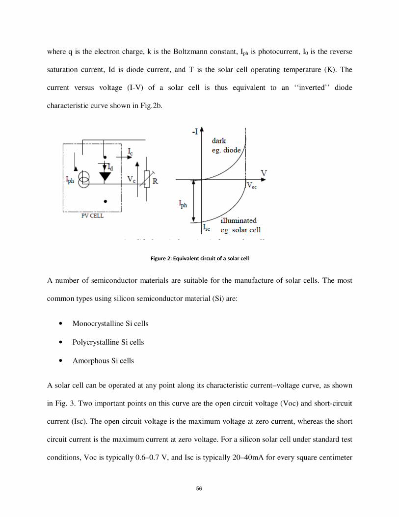
where q is the electron charge, k is the Boltzmann constant, Iph is photocurrent, I0 is the reverse
saturation current, Id is diode current, and T is the solar cell operating temperature (K). The
current versus voltage (I-V) of a solar cell is thus equivalent to an ‘‘inverted’’ diode
characteristic curve shown in Fig.2b.
Figure 2: Equivalent circuit of a solar cell
A number of semiconductor materials are suitable for the manufacture of solar cells. The most
common types using silicon semiconductor material (Si) are:
• Monocrystalline Si cells
• Polycrystalline Si cells
• Amorphous Si cells
A solar cell can be operated at any point along its characteristic current–voltage curve, as shown
in Fig. 3. Two important points on this curve are the open circuit voltage (Voc) and short-circuit
current (Isc). The open-circuit voltage is the maximum voltage at zero current, whereas the short
circuit current is the maximum current at zero voltage. For a silicon solar cell under standard test
conditions, Voc is typically 0.6–0.7 V, and Isc is typically 20–40mA for every square centimeter
56
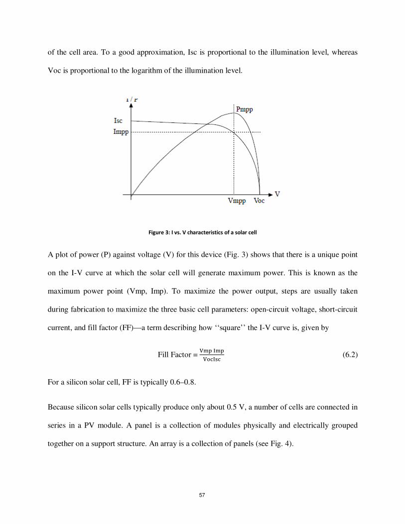
of the cell area. To a good approximation, Isc is proportional to the illumination level, whereas
Voc is proportional to the logarithm of the illumination level.
Figure 3: I vs. V characteristics of a solar cell
A plot of power (P) against voltage (V) for this device (Fig. 3) shows that there is a unique point
on the I-V curve at which the solar cell will generate maximum power. This is known as the
maximum power point (Vmp, Imp). To maximize the power output, steps are usually taken
during fabrication to maximize the three basic cell parameters: open-circuit voltage, short-circuit
current, and fill factor (FF)—a term describing how ‘‘square’’ the I-V curve is, given by
Fill Factor = V I
VI (6.2)
For a silicon solar cell, FF is typically 0.6–0.8.
Because silicon solar cells typically produce only about 0.5 V, a number of cells are connected in
series in a PV module. A panel is a collection of modules physically and electrically grouped
together on a support structure. An array is a collection of panels (see Fig. 4).
57
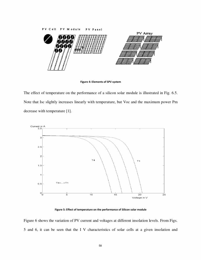
Figure 4: Elements of SPV system
The effect of temperature on the performance of a silicon solar module is illustrated in Fig. 6.5.
Note that Isc slightly increases linearly with temperature, but Voc and the maximum power Pm
decrease with temperature [1].
Figure 5: Effect of temperature on the performance of Silicon solar module
Figure 6 shows the variation of PV current and voltages at different insolation levels. From Figs.
5 and 6, it can be seen that the I V characteristics of solar cells at a given insolation and
58
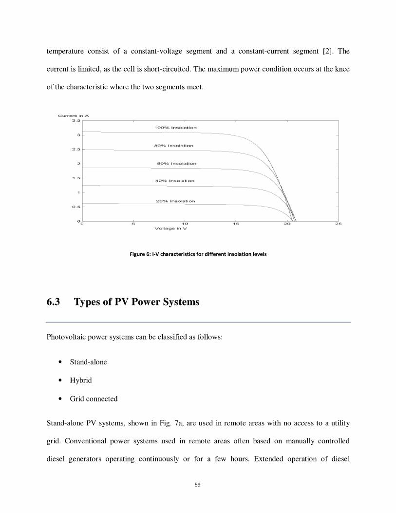
temperature consist of a constant-voltage segment and a constant-current segment [2]. The
current is limited, as the cell is short-circuited. The maximum power condition occurs at the knee
of the characteristic where the two segments meet.
Figure 6: I-V characteristics for different insolation levels
6.3 Types of PV Power Systems
Photovoltaic power systems can be classified as follows:
• Stand-alone
• Hybrid
• Grid connected
Stand-alone PV systems, shown in Fig. 7a, are used in remote areas with no access to a utility
grid. Conventional power systems used in remote areas often based on manually controlled
diesel generators operating continuously or for a few hours. Extended operation of diesel
59
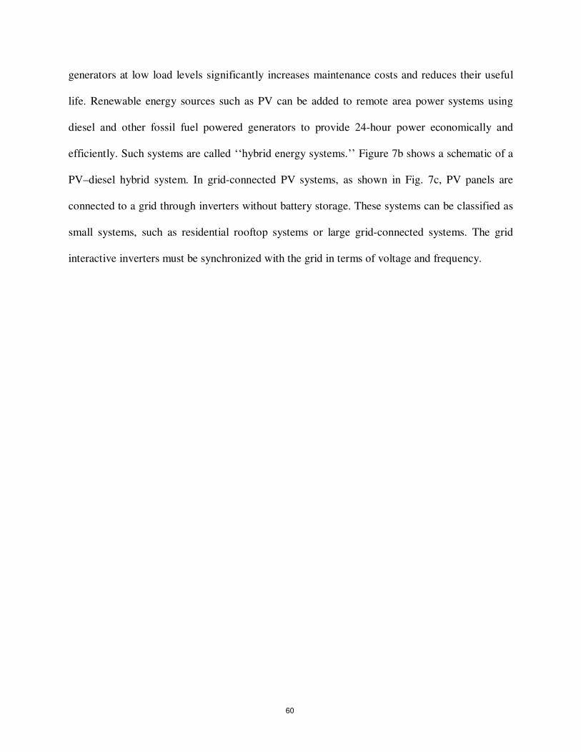
generators at low load levels significantly increases maintenance costs and reduces their useful
life. Renewable energy sources such as PV can be added to remote area power systems using
diesel and other fossil fuel powered generators to provide 24-hour power economically and
efficiently. Such systems are called ‘‘hybrid energy systems.’’ Figure 7b shows a schematic of a
PV–diesel hybrid system. In grid-connected PV systems, as shown in Fig. 7c, PV panels are
connected to a grid through inverters without battery storage. These systems can be classified as
small systems, such as residential rooftop systems or large grid-connected systems. The grid
interactive inverters must be synchronized with the grid in terms of voltage and frequency.
60
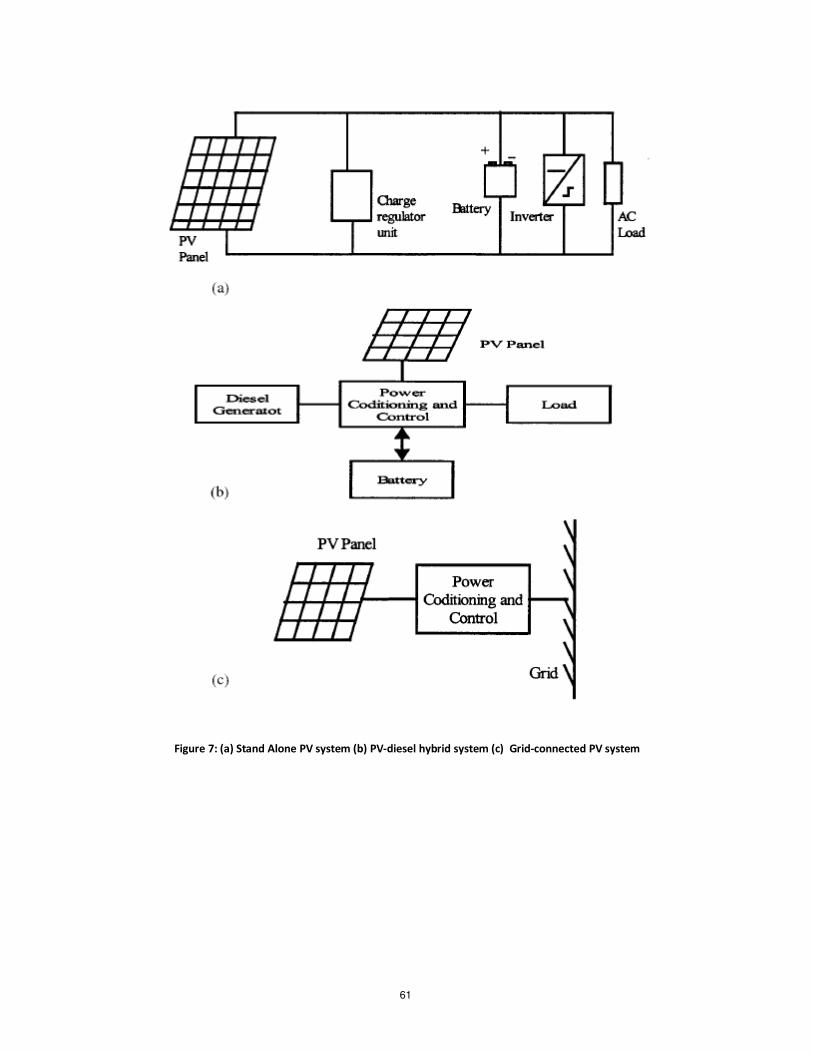
Figure 7: (a) Stand Alone PV system (b) PV-diesel hybrid system (c) Grid-connected PV system
61
6.4 Stand-Alone PV Systems
The two main stand-alone PV applications are:
• Battery charging
• Solar water pumping
6.4.1 Battery Charging
Batteries for PV Systems: A stand-alone photovoltaic energy system requires storage to meet
the energy demand during periods of low solar irradiation and nighttime. Several types of
batteries are available, such as lead-acid, nickel-cadmium, lithium, zinc bromide, zinc chloride,
sodium–sulfur, nickel–hydrogen, red-ox and vanadium batteries. The provision of cost-effective
electrical energy storage remains one of the major challenges for the development of improved
PV power systems. Typically, lead-acid batteries are used to guarantee several hours to a few
days of energy storage. Their reasonable cost and general availability has resulted in the
widespread application of lead-acid batteries for remote area power supplies despite their limited
lifetime compared to other system components. Lead acid batteries can be deep or shallow
cycling, gelled batteries, batteries with captive or liquid electrolyte, sealed and non-sealed
batteries, etc. [3]. Sealed batteries are valve regulated to permit evolution of excess hydrogen gas
(although catalytic converters are used to convert as much evolved hydrogen and oxygen back to
water as possible). Sealed batteries need less maintenance.
The following factors are considered in the selection of batteries for PV applications [1]:
• Deep discharge (70–80% depth discharge)
62
• Low charging/discharging current
• Long-duration charge (slow) and discharge (long duty cycle)
• Irregular and varying charge/discharge
• Low self-discharge
• Long lifetime
• Less maintenance requirement
• High energy storage efficiency
• Low cost
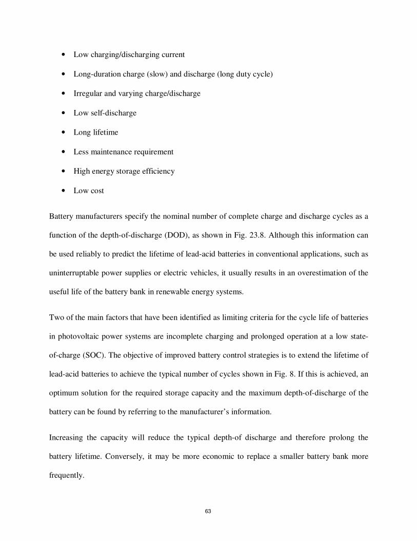
Battery manufacturers specify the nominal number of complete charge and discharge cycles as a
function of the depth-of-discharge (DOD), as shown in Fig. 23.8. Although this information can
be used reliably to predict the lifetime of lead-acid batteries in conventional applications, such as
uninterruptable power supplies or electric vehicles, it usually results in an overestimation of the
useful life of the battery bank in renewable energy systems.
Two of the main factors that have been identified as limiting criteria for the cycle life of batteries
in photovoltaic power systems are incomplete charging and prolonged operation at a low state-
of-charge (SOC). The objective of improved battery control strategies is to extend the lifetime of
lead-acid batteries to achieve the typical number of cycles shown in Fig. 8. If this is achieved, an
optimum solution for the required storage capacity and the maximum depth-of-discharge of the
battery can be found by referring to the manufacturer’s information.
Increasing the capacity will reduce the typical depth-of discharge and therefore prolong the
battery lifetime. Conversely, it may be more economic to replace a smaller battery bank more
frequently.
63
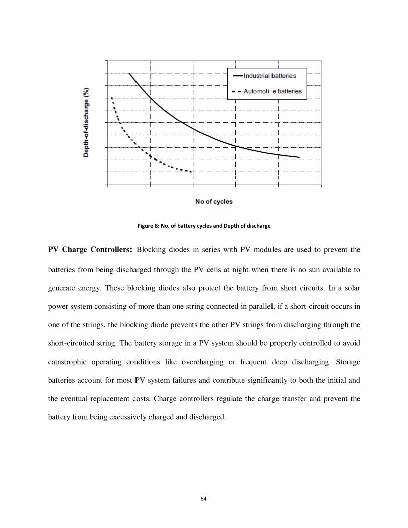
Figure 8: No. of battery cycles and Depth of discharge
PV Charge Controllers: Blocking diodes in series with PV modules are used to prevent the
batteries from being discharged through the PV cells at night when there is no sun available to
generate energy. These blocking diodes also protect the battery from short circuits. In a solar
power system consisting of more than one string connected in parallel, if a short-circuit occurs in
one of the strings, the blocking diode prevents the other PV strings from discharging through the
short-circuited string. The battery storage in a PV system should be properly controlled to avoid
catastrophic operating conditions like overcharging or frequent deep discharging. Storage
batteries account for most PV system failures and contribute significantly to both the initial and
the eventual replacement costs. Charge controllers regulate the charge transfer and prevent the
battery from being excessively charged and discharged.
64
Three types of charge controllers are commonly used:
• Series charge regulators
• Shunt charge regulators
• DC–DC Converters
Series Charge Regulators: The basic circuit for the series regulators is given in Fig. 9. In the
series charge controller, the switch S1 disconnects the PV generator when a predefined battery
voltage is achieved. When the voltage falls below the discharge limit, the load is disconnected
from the battery to avoid deep discharge beyond the limit. The main problem associated with this
type of controller is the losses associated with the switches. This extra power loss has to come
from the PV power, and this can be quite significant. Bipolar transistors, MOSFETs, or relays
are used as the switches.
Figure 9: Series Charge Regulator
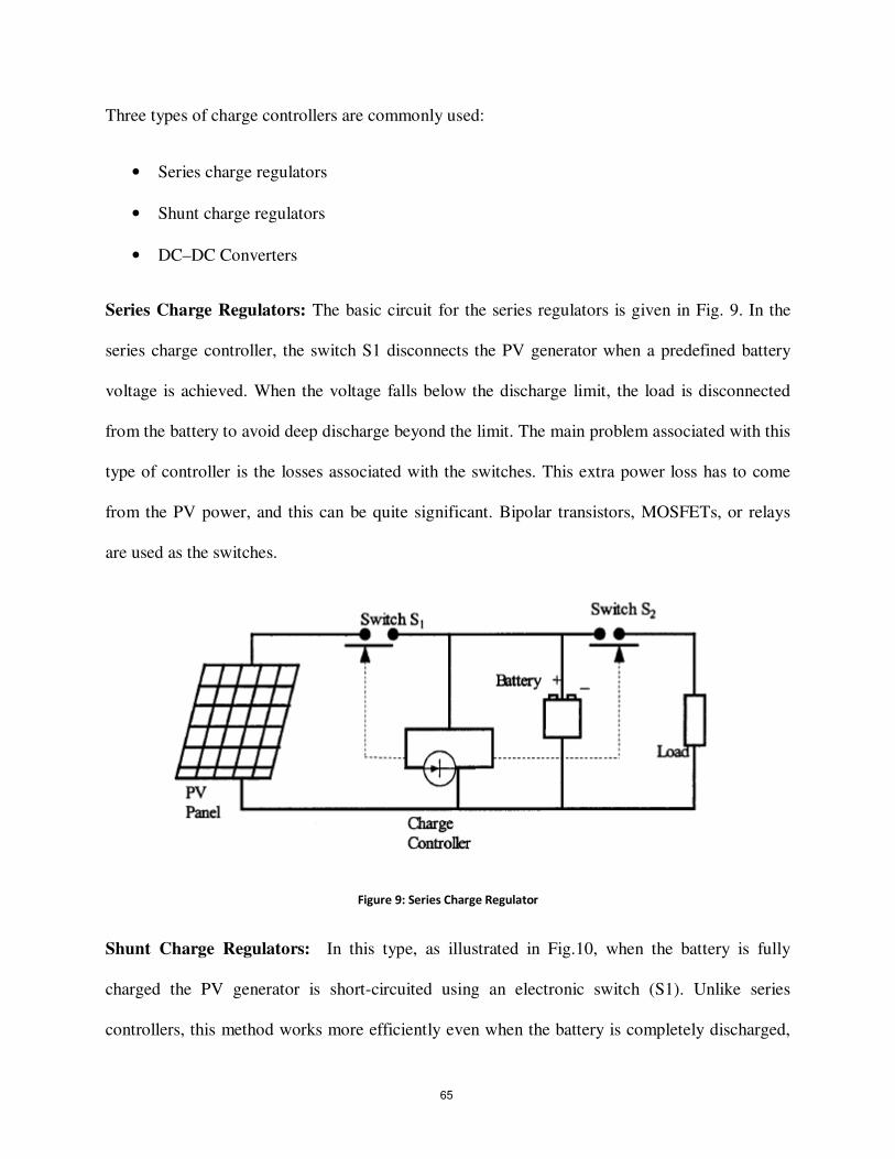
Shunt Charge Regulators: In this type, as illustrated in Fig.10, when the battery is fully
charged the PV generator is short-circuited using an electronic switch (S1). Unlike series
controllers, this method works more efficiently even when the battery is completely discharged,
65
as the short circuit switch need not be activated until the battery is fully discharged [1]. The
blocking diode prevents short-circuiting of the battery.
Shunt charge regulators are used for small PV applications (less than 20 A). Deep-discharge
protection is used to protect the battery against deep discharge. When the battery voltage reaches
below the minimum set point for the deep-discharge limit, switch S2 disconnects the load.
Simple series and shunt regulators allow only relatively coarse adjustment of the current flow
and seldom meet the exact requirements of PV systems.
Figure 10: Shunt Charge Regulators
DC–DC Converter Type Charge Regulators: Switch mode DC-to-DC converters are used to
match the output of a PV generator to a variable load. There are various types of DC–DC
converters:
• Buck (step-down) converter
• Boost (step-up) converter
66

• Buck-boost (step-down/up) converter
Figures 11a, 11b, and 11c show simplified diagrams of these three basic types of converters. The
basic concepts are an electronic switch, an inductor to store energy, and a ‘‘flywheel’’ diode,
which carries the current during that part of switching cycle when the switch is off. The DC–DC
converters allow the charge current to be reduced continuously in such a way that the resulting
battery voltage is maintained at a specified value.
Figure 11: (a) Buck Converter (b) Boost Converter (c) Buck-Boost Converter
67
6.4.2 Solar Water Pumping
In many remote and rural areas, hand pumps or diesel driven pumps are used for water supply.
Diesel pumps consume fossil fuel, affect the environment, need more maintenance, and are less
reliable. Photovoltaic (PV)-powered water pumps have received considerable attention because
of major developments in the field of solar-cell materials and power electronic systems
technology.
Types of Pumps: Two types of pumps are commonly used for water-pumping applications:
Positive displacement and centrifugal. Both centrifugal and positive displacement pumps can be
further classified into those with motors that are surface mounted, and those that are submerged
into the water (‘‘submersible’’).
Displacement pumps have water output directly proportional to the speed of the pump, but
almost independent of head. These pumps are used for solar water pumping from deep wells or
bores. They may be piston-type pumps or use a diaphragm driven by a cam or rotary screw, or
use a progressive cavity system. The pumping rate of these pumps is directly related to the speed,
and hence constant torque is desired.
Centrifugal pumps are used for low-head applications, especially if they are directly interfaced
with the solar panels. Centrifugal pumps are designed for fixed-head applications, and the
pressure difference generated increases in relation to the speed of the pump. These pumps are of
the rotating impeller type, which throws the water radially against a casing shaped so that the
momentum of the water is converted into useful pressure for lifting [3]. The centrifugal pumps
have relatively high efficiency, but it decreases at lower speeds, which can be a problem for a
solar water-pumping system at times of low light levels. The single-stage centrifugal pump has
68

just one impeller, whereas most borehole pumps are multistage types where the outlet from one
impeller goes into the center of another and each one keeps increasing the pressure difference.
From Fig. 12a, it is quite obvious that the load line is located far away from the Pmax line. It has
been reported that the daily utilization efficiency for a DC motor drive is 87% for a centrifugal
pump compared to 57% for a constant-torque characteristic load. Hence, centrifugal pumps are
more compatible with PV arrays. The system operating point is determined by the intersection of
the I V characteristic of the PV array and that of the motor, as shown in Fig. 12a. The torque-
speed slope is normally large because of the armature resistance being small. At the instant of
starting, the speed and the back emf are zero. Hence the motor starting current is approximately
the short-circuit current of the PV array. Matching the load to the PV source through a maximum
power-point tracker increases the starting torque.
The matching of a DC motor depends on the type of load being used. For instance, a centrifugal
pump is characterized by having the load torque proportional to the square of speed. The
operating characteristics of the system (i.e., PV source, PM DC motor, and load) are at the
intersection of the motor and load characteristics as shown in Fig. 12b (i.e., points a; b; c; d; e,
and f for the centrifugal pump). From Fig. 12b, the system utilizing the centrifugal pump as its
load tends to start at low solar irradiation (point a) level. However, for systems with an almost
constant torque characteristic (Fig.12(b), line 1), the start is at almost 50% of one sun (full
insolation), which results in a short period of operation.
69
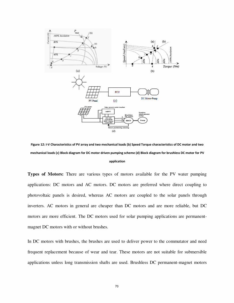
Figure 12: I-V Characteristics of PV array and two mechanical loads (b) Speed Torque characteristics of DC motor and two
mechanical loads (c) Block diagram for DC motor driven pumping scheme (d) Block diagram for brushless DC motor for PV
application
Types of Motors: There are various types of motors available for the PV water pumping
applications: DC motors and AC motors. DC motors are preferred where direct coupling to
photovoltaic panels is desired, whereas AC motors are coupled to the solar panels through
inverters. AC motors in general are cheaper than DC motors and are more reliable, but DC
motors are more efficient. The DC motors used for solar pumping applications are permanent-
magnet DC motors with or without brushes.
In DC motors with brushes, the brushes are used to deliver power to the commutator and need
frequent replacement because of wear and tear. These motors are not suitable for submersible
applications unless long transmission shafts are used. Brushless DC permanent-magnet motors
70
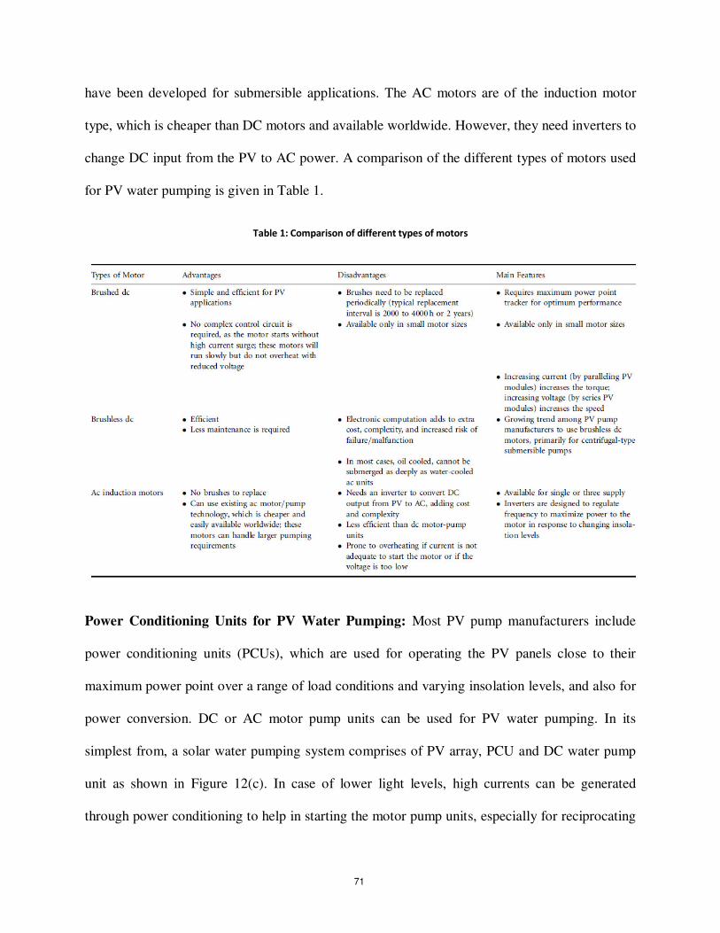
have been developed for submersible applications. The AC motors are of the induction motor
type, which is cheaper than DC motors and available worldwide. However, they need inverters to
change DC input from the PV to AC power. A comparison of the different types of motors used
for PV water pumping is given in Table 1.
Table 1: Comparison of different types of motors
Power Conditioning Units for PV Water Pumping: Most PV pump manufacturers include
power conditioning units (PCUs), which are used for operating the PV panels close to their
maximum power point over a range of load conditions and varying insolation levels, and also for
power conversion. DC or AC motor pump units can be used for PV water pumping. In its
simplest from, a solar water pumping system comprises of PV array, PCU and DC water pump
unit as shown in Figure 12(c). In case of lower light levels, high currents can be generated
through power conditioning to help in starting the motor pump units, especially for reciprocating
71
positive-displacement type pumps with constant torque characteristics requiring constant current
throughout the operating region. In positive- displacement type pumps, the torque generated by
the pumps depends on the pumping head, friction, pipe diameter, etc., and requires a certain level
of current to produce the necessary torque. Some systems use electronic controllers to assist in
starting and operating the motor under low solar radiation. This is particularly important when
using positive displacement pumps. The solar panels generate DC voltage and current. Solar
water pumping systems usually have DC or AC pumps. For DC pumps, the PV output can be
directly connected to the pump through maximum power point tracker, or a DC–DC converter
can also be used for interfacing for controlled DC output from PV panels. To feed the ac motors,
a suitable interface is required for the power conditioning. These PV inverters for the stand-alone
applications are very expensive. The aim of power conditioning equipment is to supply the
controlled voltage/current output from the converters/inverters to the motor-pump unit.
These power-conditioning units are also used for operating the PV panels close to their
maximum efficiency for fluctuating solar conditions. The speed of the pump is governed by the
available driving voltage. If current becomes lower than the acceptable limit, then the pumping
will stop. When the light level increases, the operating point will shift from the maximum-power
point leading to a reduction in efficiency. For centrifugal pumps, there is an increase in current at
increased speed, and the matching of I V characteristics is closer for a wide range of light
intensity levels. For centrifugal pumps, the torque is proportional to the square of the speed, and
the torque produced by the motors is proportional to the current. Because of the decrease in PV
current output, the torque from the motor and consequently the speed of the pump are reduced,
resulting in a decrease in back emf and the required voltage for the motor. A maximum-power-
point tracker (MPPT) can be used for controlling the voltage=current outputs from the PV
72
inverters to operate the PV close to the maximum operating point for smooth operation of
motorpump units. The DC–DC converter can be used to keep the PVpanel output voltage
constant and to help in operating the solar arrays close to the maximum-power point. In the
beginning, a high starting current is required to produce a high starting torque. The PV panels
cannot supply this high starting current without adequate power conditioning equipment such as
a DC–DC converter or by using a starting capacitor. The DC–DC converter can generate the high
starting currents by regulating the excess PV array voltage. The DC–DC converter can be a boost
or buck converter.
Brushless DC motors (BDCM) and helical rotor pumps can also be used for PV water pumping
[20]. BDCMs are a self-synchronous type of motor characterized by trapezoidal waveforms for
back emf and air flux density. They can operate off a low-voltage DC supply that is switched
through an inverter to create a rotating stator field. The current generation of BDCMs use rare
earth magnets on the rotor to give high airgap flux densities and are well suited to solar
application. The block diagram of such an arrangement, shown in Fig. 12d, consists of PV
panels, a DC–DC converter, an MPPT, and a brushless DC motor.
The PV inverters are used to convert the DC output of the solar arrays to an AC quantity so as to
run the ac motor-driven pumps. These PV inverters can be of the variable-frequency type, which
can be controlled to operate the motors over a wide range of loads. The PV inverters may involve
impedance matching to match the electrical characteristics of the load and array. The motor–
pump unit and PV panels operate at their maximum efficiencies [7]. The MPPT is also used in
the power conditioning. To keep the voltage stable for the inverters, the DC–DC converter can
be used. The inverter/converter has the capability of injecting high-switch-frequency
components, which can lead to overheating and losses, care must be taken in doing this. The PV
73
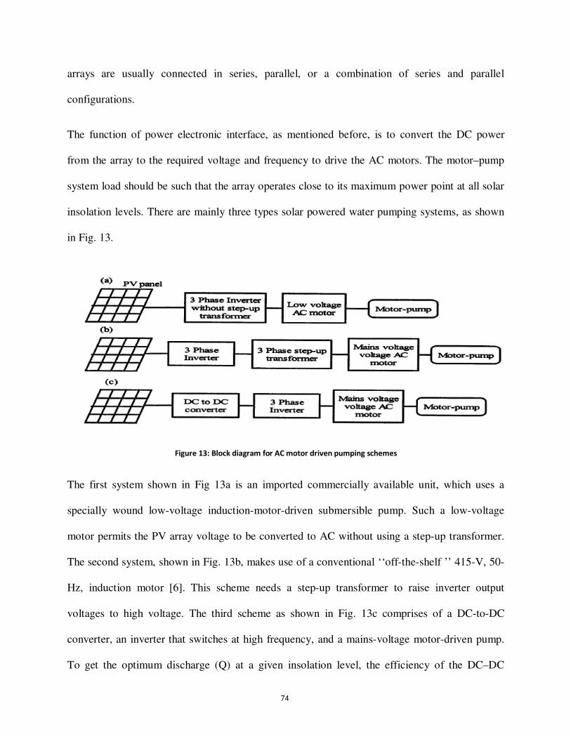
arrays are usually connected in series, parallel, or a combination of series and parallel
configurations.
The function of power electronic interface, as mentioned before, is to convert the DC power
from the array to the required voltage and frequency to drive the AC motors. The motor–pump
system load should be such that the array operates close to its maximum power point at all solar
insolation levels. There are mainly three types solar powered water pumping systems, as shown
in Fig. 13.
Figure 13: Block diagram for AC motor driven pumping schemes
The first system shown in Fig 13a is an imported commercially available unit, which uses a
specially wound low-voltage induction-motor-driven submersible pump. Such a low-voltage
motor permits the PV array voltage to be converted to AC without using a step-up transformer.
The second system, shown in Fig. 13b, makes use of a conventional ‘‘off-the-shelf ’’ 415-V, 50-
Hz, induction motor [6]. This scheme needs a step-up transformer to raise inverter output
voltages to high voltage. The third scheme as shown in Fig. 13c comprises of a DC-to-DC
converter, an inverter that switches at high frequency, and a mains-voltage motor-driven pump.
To get the optimum discharge (Q) at a given insolation level, the efficiency of the DC–DC
74
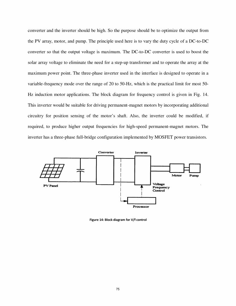
converter and the inverter should be high. So the purpose should be to optimize the output from
the PV array, motor, and pump. The principle used here is to vary the duty cycle of a DC-to-DC
converter so that the output voltage is maximum. The DC-to-DC converter is used to boost the
solar array voltage to eliminate the need for a step-up transformer and to operate the array at the
maximum power point. The three-phase inverter used in the interface is designed to operate in a
variable-frequency mode over the range of 20 to 50-Hz, which is the practical limit for most 50-
Hz induction motor applications. The block diagram for frequency control is given in Fig. 14.
This inverter would be suitable for driving permanent-magnet motors by incorporating additional
circuitry for position sensing of the motor’s shaft. Also, the inverter could be modified, if
required, to produce higher output frequencies for high-speed permanent-magnet motors. The
inverter has a three-phase full-bridge configuration implemented by MOSFET power transistors.
Figure 14: Block diagram for V/f control
75
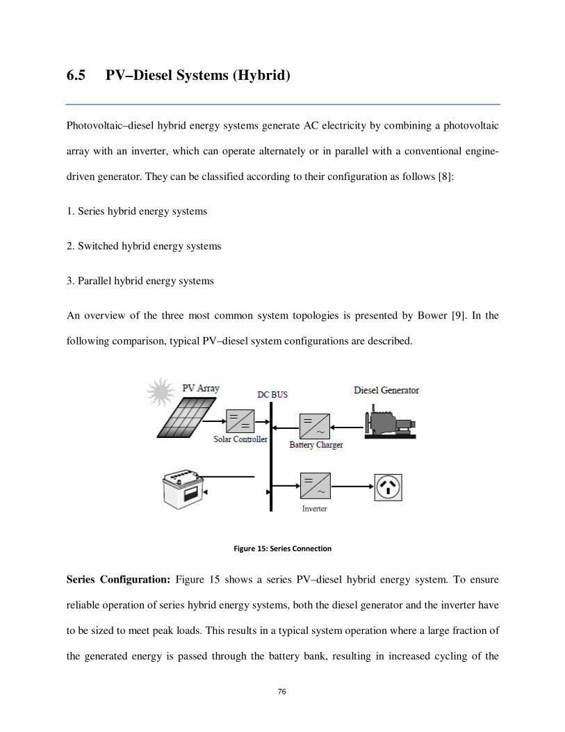
6.5 PV–Diesel Systems (Hybrid)
Photovoltaic–diesel hybrid energy systems generate AC electricity by combining a photovoltaic
array with an inverter, which can operate alternately or in parallel with a conventional engine-
driven generator. They can be classified according to their configuration as follows [8]:
1. Series hybrid energy systems
2. Switched hybrid energy systems
3. Parallel hybrid energy systems
An overview of the three most common system topologies is presented by Bower [9]. In the
following comparison, typical PV–diesel system configurations are described.
Figure 15: Series Connection
Series Configuration: Figure 15 shows a series PV–diesel hybrid energy system. To ensure
reliable operation of series hybrid energy systems, both the diesel generator and the inverter have
to be sized to meet peak loads. This results in a typical system operation where a large fraction of
the generated energy is passed through the battery bank, resulting in increased cycling of the
76
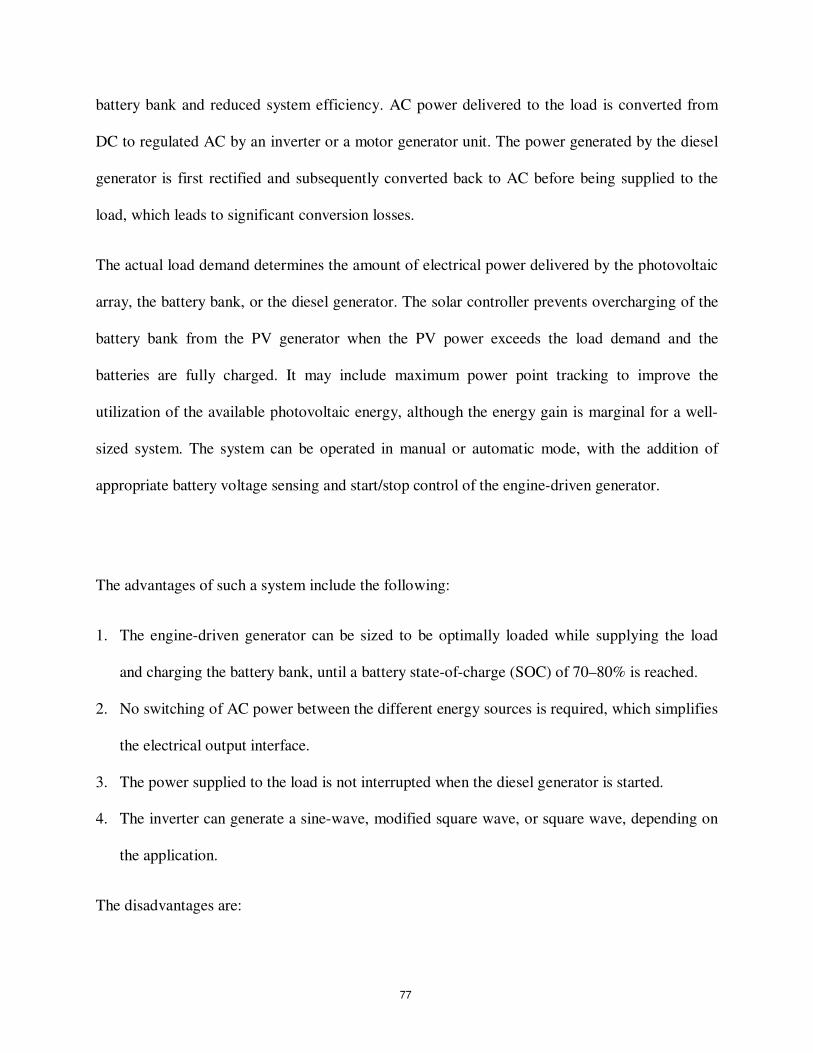
battery bank and reduced system efficiency. AC power delivered to the load is converted from
DC to regulated AC by an inverter or a motor generator unit. The power generated by the diesel
generator is first rectified and subsequently converted back to AC before being supplied to the
load, which leads to significant conversion losses.
The actual load demand determines the amount of electrical power delivered by the photovoltaic
array, the battery bank, or the diesel generator. The solar controller prevents overcharging of the
battery bank from the PV generator when the PV power exceeds the load demand and the
batteries are fully charged. It may include maximum power point tracking to improve the
utilization of the available photovoltaic energy, although the energy gain is marginal for a well-
sized system. The system can be operated in manual or automatic mode, with the addition of
appropriate battery voltage sensing and start/stop control of the engine-driven generator.
The advantages of such a system include the following:
1. The engine-driven generator can be sized to be optimally loaded while supplying the load
and charging the battery bank, until a battery state-of-charge (SOC) of 70–80% is reached.
2. No switching of AC power between the different energy sources is required, which simplifies
the electrical output interface.
3. The power supplied to the load is not interrupted when the diesel generator is started.
4. The inverter can generate a sine-wave, modified square wave, or square wave, depending on
the application.
The disadvantages are:
77
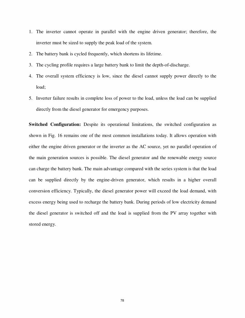
1. The inverter cannot operate in parallel with the engine driven generator; therefore, the
inverter must be sized to supply the peak load of the system.
2. The battery bank is cycled frequently, which shortens its lifetime.
3. The cycling profile requires a large battery bank to limit the depth-of-discharge.
4. The overall system efficiency is low, since the diesel cannot supply power directly to the
load;
5. Inverter failure results in complete loss of power to the load, unless the load can be supplied
directly from the diesel generator for emergency purposes.
Switched Configuration: Despite its operational limitations, the switched configuration as
shown in Fig. 16 remains one of the most common installations today. It allows operation with
either the engine driven generator or the inverter as the AC source, yet no parallel operation of
the main generation sources is possible. The diesel generator and the renewable energy source
can charge the battery bank. The main advantage compared with the series system is that the load
can be supplied directly by the engine-driven generator, which results in a higher overall
conversion efficiency. Typically, the diesel generator power will exceed the load demand, with
excess energy being used to recharge the battery bank. During periods of low electricity demand
the diesel generator is switched off and the load is supplied from the PV array together with
stored energy.
78
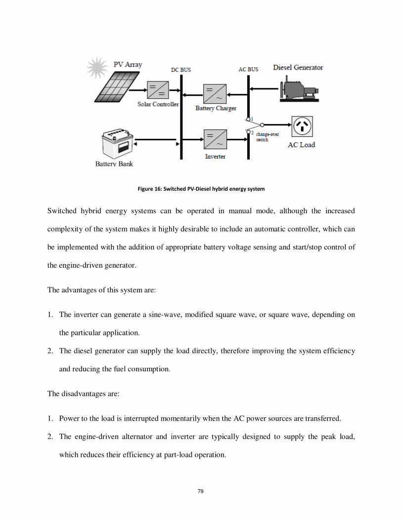
Figure 16: Switched PV-Diesel hybrid energy system
Switched hybrid energy systems can be operated in manual mode, although the increased
complexity of the system makes it highly desirable to include an automatic controller, which can
be implemented with the addition of appropriate battery voltage sensing and start/stop control of
the engine-driven generator.
The advantages of this system are:
1. The inverter can generate a sine-wave, modified square wave, or square wave, depending on
the particular application.
2. The diesel generator can supply the load directly, therefore improving the system efficiency
and reducing the fuel consumption.
The disadvantages are:
1. Power to the load is interrupted momentarily when the AC power sources are transferred.
2. The engine-driven alternator and inverter are typically designed to supply the peak load,
which reduces their efficiency at part-load operation.
79
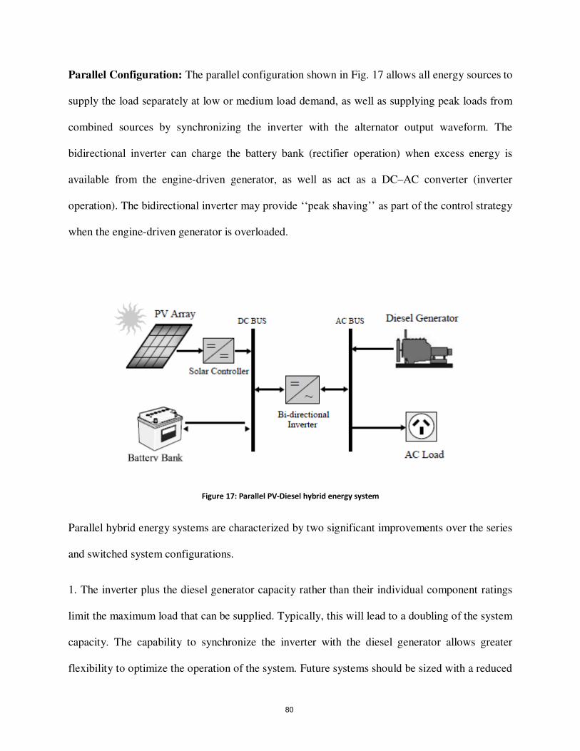
Parallel Configuration: The parallel configuration shown in Fig. 17 allows all energy sources to
supply the load separately at low or medium load demand, as well as supplying peak loads from
combined sources by synchronizing the inverter with the alternator output waveform. The
bidirectional inverter can charge the battery bank (rectifier operation) when excess energy is
available from the engine-driven generator, as well as act as a DC–AC converter (inverter
operation). The bidirectional inverter may provide ‘‘peak shaving’’ as part of the control strategy
when the engine-driven generator is overloaded.
Figure 17: Parallel PV-Diesel hybrid energy system
Parallel hybrid energy systems are characterized by two significant improvements over the series
and switched system configurations.
1. The inverter plus the diesel generator capacity rather than their individual component ratings
limit the maximum load that can be supplied. Typically, this will lead to a doubling of the system
capacity. The capability to synchronize the inverter with the diesel generator allows greater
flexibility to optimize the operation of the system. Future systems should be sized with a reduced
80
peak capacity of the diesel generator, which results in a higher fraction of directly used energy
and hence higher system efficiencies.
2. By using the same power electronic devices for both inverter and rectifier operation, the
number of system components is minimized. Additionally, wiring and system installation costs
are reduced through the integration of all power conditioning devices in one central power unit.
This highly integrated system concept has advantages over a more modular approach to system
design, but it may prevent convenient system upgrades when the load demand increases.
The parallel configuration offers a number of potential advantages over other system
configurations. These objectives can only be met if the interactive operation of the individual
components is controlled by an ‘‘intelligent’’ hybrid energy management system. Although
today’s generation of parallel systems includes system controllers of varying complexity and
sophistication, they do not optimize the performance of the complete system. Typically, both the
diesel generator and the inverter are sized to supply anticipated peak loads. As a result, most
parallel hybrid energy systems do not utilize their capability of parallel, synchronized operation
of multiple power sources.
The advantages of this system include the following:
1. The system load can be met in an optimal way.
2. Diesel generator efficiency can be maximized.
3. Diesel generator maintenance can be minimized.
4. A reduction in the rated capacities of the diesel generator, battery bank, inverter, and
renewable resources is feasible, while also meeting the peak loads.
The disadvantages are:
81
1. Automatic control is essential for the reliable operation of the system.
2. The inverter has to be a true sine-wave inverter with the ability to synchronize with a
secondary AC source.
3. System operation is less transparent to the untrained user of the system.
6.6 Control of PV–Diesel Hybrid Systems
The design process of hybrid energy systems requires the selection of the most suitable
combination of energy sources, power-conditioning devices, and energy-storage system, together
with the implementation of an efficient energy dispatch strategy. System simulation software is
an essential tool to analyze and compare possible system combinations. The objective of the
control strategy is to achieve optimal operational performance at the system level. Inefficient
operation of the diesel generator and ‘‘dumping’’ of excess energy is common for many remote-
area power supplies operating in the field. Component maintenance and replacement contributes
significantly to the life-cycle cost of systems. These aspects of system operation are clearly
related to the selected control strategy and have to be considered in the system design phase.
Advanced system control strategies seek to reduce the number of cycles and the depth-of-
discharge for the battery bank, run the diesel generator in its most efficient operating range,
maximize the utilization of the renewable resource, and ensure high reliability of the system.
Because of the varying nature of the load demand, the fluctuating power supplied by the
photovoltaic generator, and the resulting variation of battery SOC, the hybrid energy system
controller has to respond to continuously changing operating conditions.
82
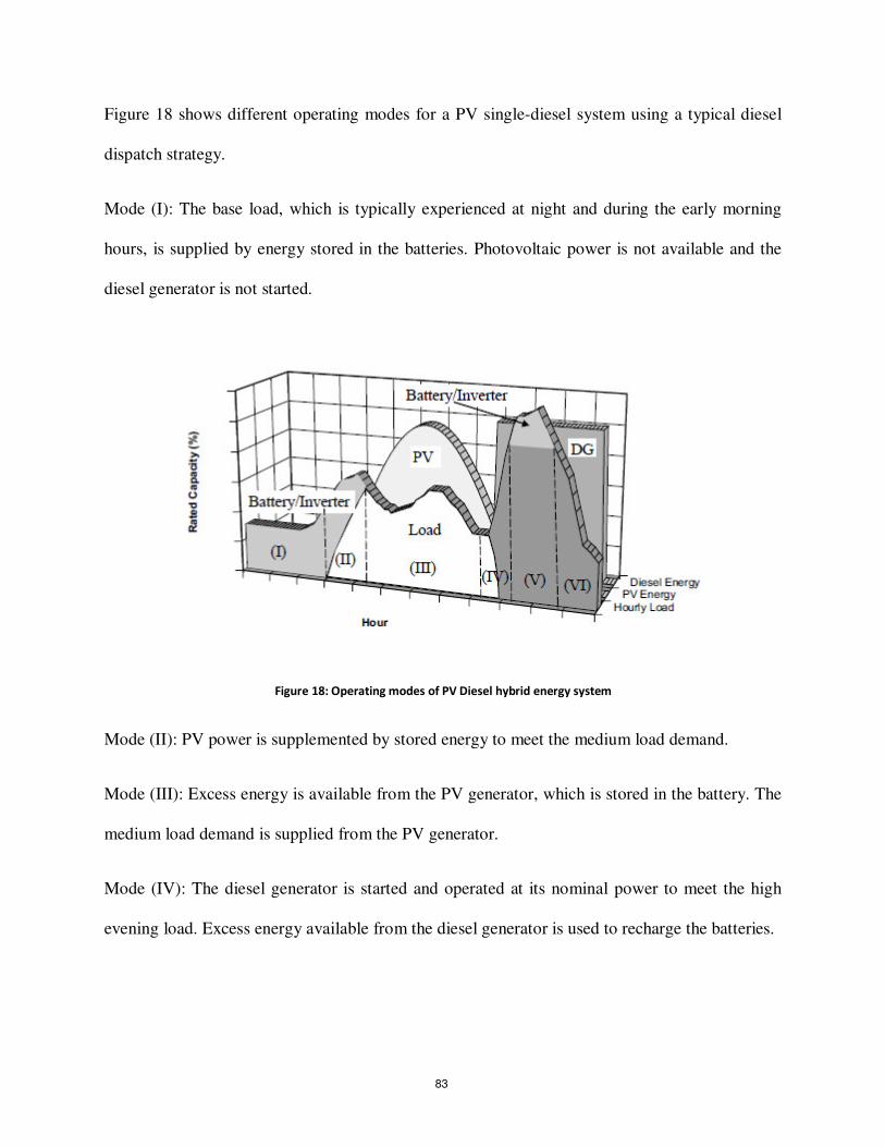
Figure 18 shows different operating modes for a PV single-diesel system using a typical diesel
dispatch strategy.
Mode (I): The base load, which is typically experienced at night and during the early morning
hours, is supplied by energy stored in the batteries. Photovoltaic power is not available and the
diesel generator is not started.
Figure 18: Operating modes of PV Diesel hybrid energy system
Mode (II): PV power is supplemented by stored energy to meet the medium load demand.
Mode (III): Excess energy is available from the PV generator, which is stored in the battery. The
medium load demand is supplied from the PV generator.
Mode (IV): The diesel generator is started and operated at its nominal power to meet the high
evening load. Excess energy available from the diesel generator is used to recharge the batteries.
83

Mode (V): The diesel generator power is insufficient to meet the peak load demand. Additional
power is supplied from the batteries by synchronizing the inverter AC output voltage with the
alternator waveform.
Mode (VI): The diesel generator power exceeds the load demand, but it is kept operational until
the batteries are recharged to a high state-of-charge level.
In principle, most efficient operation is achieved if the generated power is supplied directly to the
load from all energy sources, which also reduces cycling of the battery bank. However, since
diesel generator operation at light loads is inherently inefficient, it is common practice to operate
the engine-driven generator at its nominal power rating and to recharge the batteries from the
excess energy. The selection of the most efficient control strategy depends on fuel, maintenance
and component-replacement cost, the system configuration, and environmental conditions, as
well as constraints imposed on the operation of the hybrid energy system.
84
6.7 Grid Connected PV Systems
Utility interactive inverters not only condition the power output of the photovoltaic arrays but
ensure that the PV system output is fully synchronized with the utility power. These systems can
be battery-less or with battery backup. Systems with battery storage (or a flywheel) provide
additional power-supply reliability. The grid connection of photovoltaic systems is gathering
momentum because of various rebate and incentive schemes. This system allows the consumer to
feed its own load utilizing the available solar energy, and the surplus energy can be injected into
the grid under the energy buy-back scheme to reduce the payback period. Grid-connected PV
systems can become a part of the utility system. The contribution of solar power depends on the
size of system and the load curve of the house. When the PV system is integrated with the utility
grid, a two-way power flow is established. The utility grid will absorb excess PV power and will
feed the house at night and at instants when the PV power is inadequate. The utility companies
are encouraging this scheme in many parts of the world. The grid-connected system can be
classified as follows:
• Rooftop application of grid-connected PV system
• Utility-scale large system
For small household PV applications, a roof-mounted PV array can be the best option. Solar cells
provide an environmentally clean way of producing electricity, and rooftops have always been
the ideal place to put them. With a PV array on the rooftop, the solar-generated power can supply
residential load. The rooftop PV systems can help in reducing the peak summer load to the
benefit of utility companies by feeding the household lighting, cooling, and other domestic loads.
The battery storage can further improve the reliability of the system at times of low insolation
85
level, at night or on cloudy days. But the battery storage has some inherent problems, such as
maintenance and higher cost. For roof-integrated applications, the solar arrays can be either
mounted on the roof or directly integrated into the roof. If the roof integration does not allow for
an air channel behind the PV modules for ventilation purposes, then it can increase the cell
temperature during the operation, consequently leading to some energy losses. The disadvantage
of the rooftop application is that the PV array orientation is dictated by the roof. In cases, where
the roof orientation differs from the optimal orientation required for the cells, the efficiency of
the entire system would be suboptimal.
Utility interest in PV has centered on the large grid connected PV systems. In Germany, the
United States, Spain, and several other parts of the world, some large PV-scale plants have been
installed. The utilities are more inclined toward large-scale, centralized power supplies. The PV
systems can be centralized or distributed systems.
Grid-connected PV systems must observe the islanding situation, when the utility supply fails. In
case of islanding, the PV generators should be disconnected from mains. PV generators can
continue to meet only the local load, if the PV output matches the load. If the grid is reconnected
during islanding, transient over-currents can flow through the PV system inverters, and
protective equipment such as circuit breakers may be damaged. Islanding control can be
achieved through inverters or via the distribution network. Inverter controls can be designed on
the basis of detection of grid voltage or measurement of impedance, frequency variation, or
increase in harmonics. Protection must be designed for islanding, short circuits, over=under
voltages/currents, grounding and lightning etc.
86
The importance of the power generated by the PV system depends on the time of the day,
especially when the utility is experiencing peak load. The PV plants are well suited to summer
peaking, but it depends upon the climatic condition of the site. PV systems being investigated for
use as peaking stations would be competitive for load management. The PV users can defer their
load by adopting load management to get the maximum benefit out of the grid-connected PV
plants and feeding more power into the grid at the time of peak load.
The assigned capacity credit is based on the statistical probability that the grid can meet peak
demand [3]. The capacity factor during peaks is very similar to that of conventional plants, and
similar capacity credit can be given for PV generation, except at times when the PV plants are
generating very much less power, unless adequate storage is provided.
With the installation of PV plants, the need for extra transmission lines and transformers can be
delayed or avoided. The distributed PV plants can also contribute in providing reactive power
support to the grid and reduce the burden on VAR compensators.
6.7.1 Inverters for Grid-Connected Applications
The power conditioner is the key link between the PV array and mains in the grid-connected PV
system. It acts as an interface that converts DC current produced by the solar cells into utility-
grade AC current. The PV system behavior relies heavily on the power-conditioning unit. The
inverters must produce good-quality sine-wave output, must follow the frequency and voltage of
the grid, and must extract maximum power from the solar cells with the help of a maximum-
power point tracker. The inverter input stage varies the input voltage until the maximum power
point on the I V curve is found. The inverter must monitor all the phases of the grid, and inverter
output must be controlled in terms of voltage and frequency variation. A typical grid-connected
87
inverter may use a pulse-width modulation (PWM) scheme and operate in the range of 2 kHz up
to 20 kHz.
6.7.2 Inverter Classifications
The inverters used for grid interfacing are broadly classified as voltage-source inverters (VSI)
and current-source inverters (CSI); whereas the inverters based on the control schemes can be
classified as current-controlled inverters (CCI) and voltage-controlled inverters (VCI). The
source is not necessarily characterized by the energy source for the system. It is a characteristic
of the topology of the inverter. It is possible to change from one source type to another source
type by the addition of passive components. In the voltage-source inverter (VSI), the DC side is
made to appear to the inverter as a voltage source. The voltage-source inverters have a capacitor
in parallel across the input, whereas the current-source inverters have an inductor in series with
the DC input. In the current source inverter (CSI), the DC source appears as a current source to
the inverter. Solar arrays are fairly good approximation to a current source. Most PV inverters
are voltage source, even though the PV is a current source. Current-source inverters are generally
used for large motor drives although there have been some PV inverters built using a current
source topology. The voltage-source inverter is more popular, with the PWM voltage-source
inverter (VSI) dominating the sine-wave inverter topologies.
88
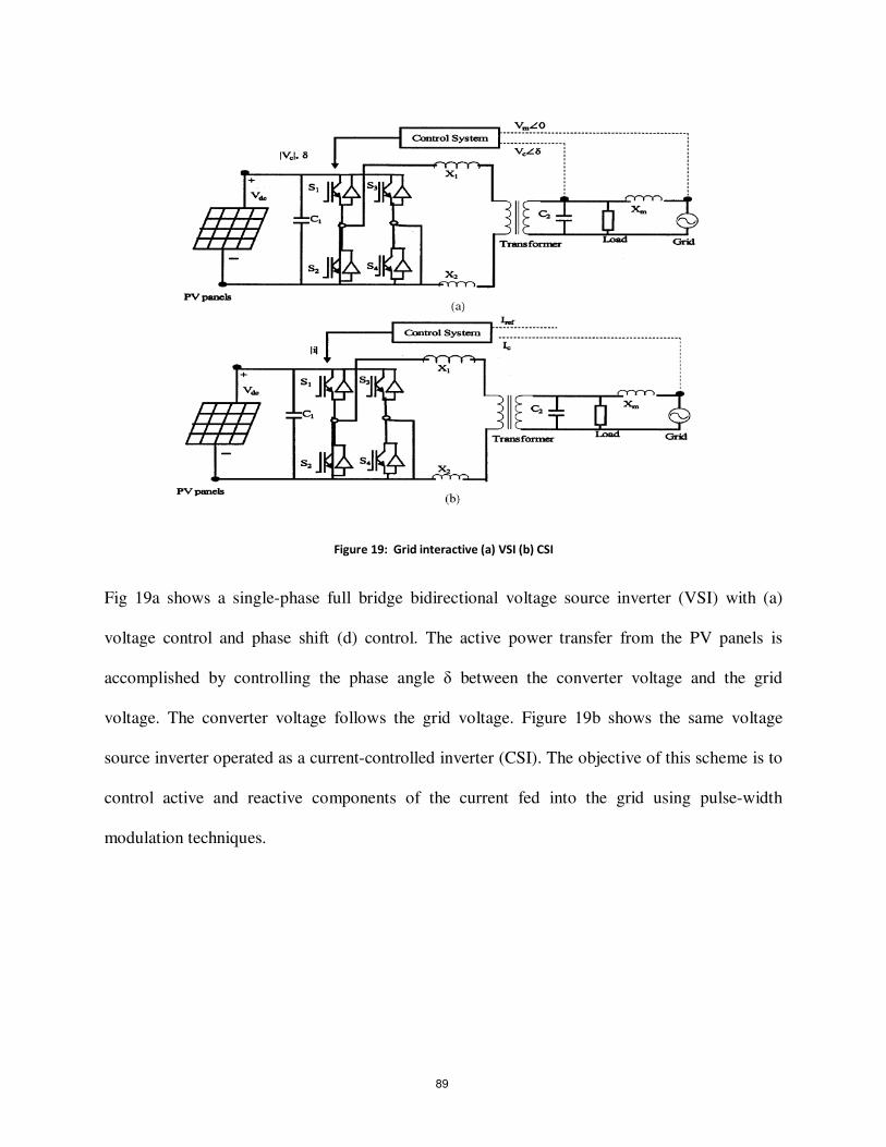
Figure 19: Grid interactive (a) VSI (b) CSI
Fig 19a shows a single-phase full bridge bidirectional voltage source inverter (VSI) with (a)
voltage control and phase shift (d) control. The active power transfer from the PV panels is
accomplished by controlling the phase angle δ between the converter voltage and the grid
voltage. The converter voltage follows the grid voltage. Figure 19b shows the same voltage
source inverter operated as a current-controlled inverter (CSI). The objective of this scheme is to
control active and reactive components of the current fed into the grid using pulse-width
modulation techniques.
89
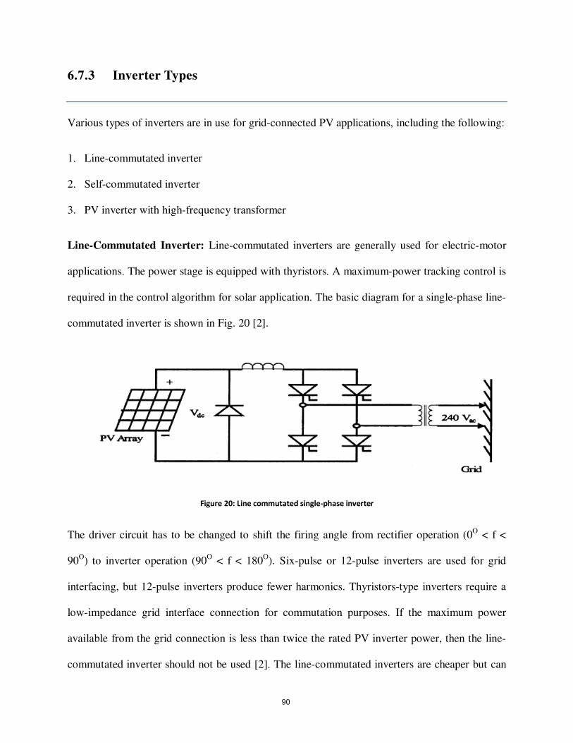
6.7.3 Inverter Types
Various types of inverters are in use for grid-connected PV applications, including the following:
1. Line-commutated inverter
2. Self-commutated inverter
3. PV inverter with high-frequency transformer
Line-Commutated Inverter: Line-commutated inverters are generally used for electric-motor
applications. The power stage is equipped with thyristors. A maximum-power tracking control is
required in the control algorithm for solar application. The basic diagram for a single-phase line-
commutated inverter is shown in Fig. 20 [2].
Figure 20: Line commutated single-phase inverter
The driver circuit has to be changed to shift the firing angle from rectifier operation (0O < f <
90O) to inverter operation (90
O < f < 180
O). Six-pulse or 12-pulse inverters are used for grid
interfacing, but 12-pulse inverters produce fewer harmonics. Thyristors-type inverters require a
low-impedance grid interface connection for commutation purposes. If the maximum power
available from the grid connection is less than twice the rated PV inverter power, then the line-
commutated inverter should not be used [2]. The line-commutated inverters are cheaper but can
90
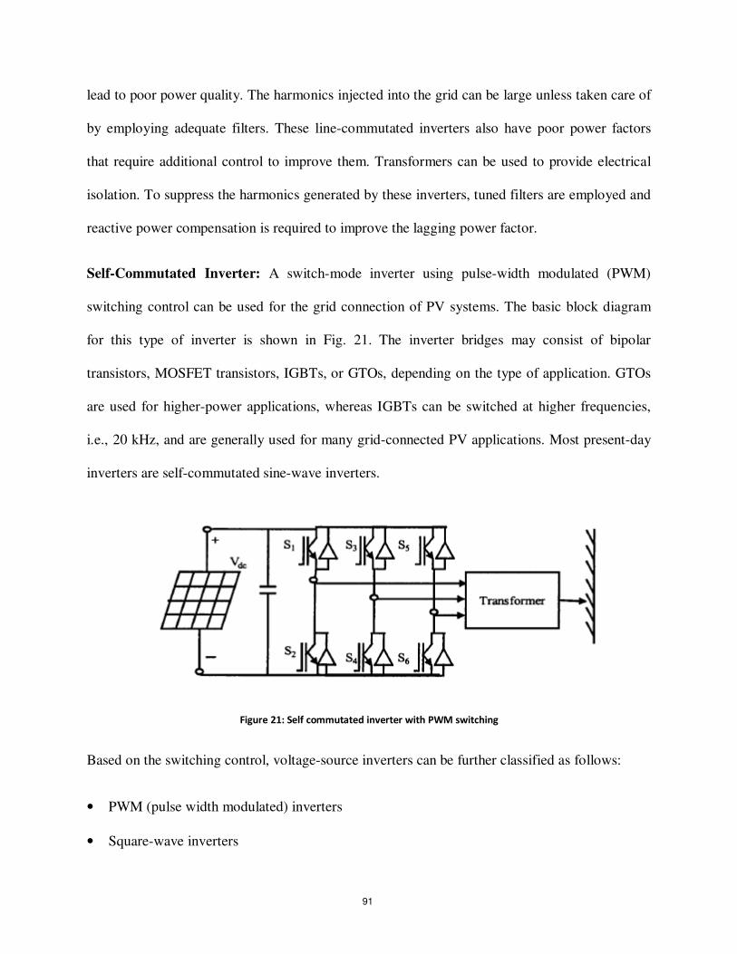
lead to poor power quality. The harmonics injected into the grid can be large unless taken care of
by employing adequate filters. These line-commutated inverters also have poor power factors
that require additional control to improve them. Transformers can be used to provide electrical
isolation. To suppress the harmonics generated by these inverters, tuned filters are employed and
reactive power compensation is required to improve the lagging power factor.
Self-Commutated Inverter: A switch-mode inverter using pulse-width modulated (PWM)
switching control can be used for the grid connection of PV systems. The basic block diagram
for this type of inverter is shown in Fig. 21. The inverter bridges may consist of bipolar
transistors, MOSFET transistors, IGBTs, or GTOs, depending on the type of application. GTOs
are used for higher-power applications, whereas IGBTs can be switched at higher frequencies,
i.e., 20 kHz, and are generally used for many grid-connected PV applications. Most present-day
inverters are self-commutated sine-wave inverters.
Figure 21: Self commutated inverter with PWM switching
Based on the switching control, voltage-source inverters can be further classified as follows:
• PWM (pulse width modulated) inverters
• Square-wave inverters
91

• Single-phase inverters with voltage cancellations
• Programmed harmonic elimination switching
• Current-controlled modulation
PV Inverter with High-Frequency Transformer: The 50-Hz transformer for a standard PV
inverter with PWM switching scheme can be very heavy and costly. When using frequencies
more than 20 kHz, a ferrite core transformer can be a better option [2]. A circuit diagram of a
grid connected PV system using high frequency transformer is shown in Fig. 22.
The capacitor on the input side of the high-frequency inverter acts as a filter. The high-frequency
inverter with pulse-width modulation is used to produce a high-frequency AC across the primary
winding of the high-frequency transformer. The secondary voltage of this transformer is rectified
using a high-frequency rectifier. The DC voltage is interfaced with a thyristor inverter through a
low-pass inductor filter and hence connected to the grid. The line current is required to be
sinusoidal and in phase with the line voltage. To achieve this, the line voltage (V1) is measured
to establish the reference waveform for the line current IL*. This reference current IL
* multiplied
by the transformer ratio gives the reference current at the output of the high-frequency inverter.
The inverter output can be controlled using current-controls technique [10]. These inverters can
be used with low-frequency or high-frequency transformer isolation. The low-frequency (50/60
Hz) transformer of a standard inverter with pulse-width modulation is a very heavy and bulky
component. For residential grid interactive rooftop inverters below 3-kW rating, high-frequency
transformer isolation is often preferred.
92
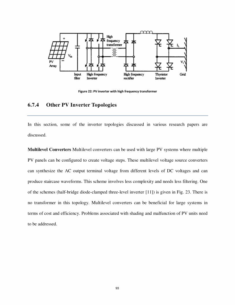
Figure 22: PV inverter with high frequency transformer
6.7.4 Other PV Inverter Topologies
In this section, some of the inverter topologies discussed in various research papers are
discussed.
Multilevel Converters Multilevel converters can be used with large PV systems where multiple
PV panels can be configured to create voltage steps. These multilevel voltage source converters
can synthesize the AC output terminal voltage from different levels of DC voltages and can
produce staircase waveforms. This scheme involves less complexity and needs less filtering. One
of the schemes (half-bridge diode-clamped three-level inverter [11]) is given in Fig. 23. There is
no transformer in this topology. Multilevel converters can be beneficial for large systems in
terms of cost and efficiency. Problems associated with shading and malfunction of PV units need
to be addressed.
93
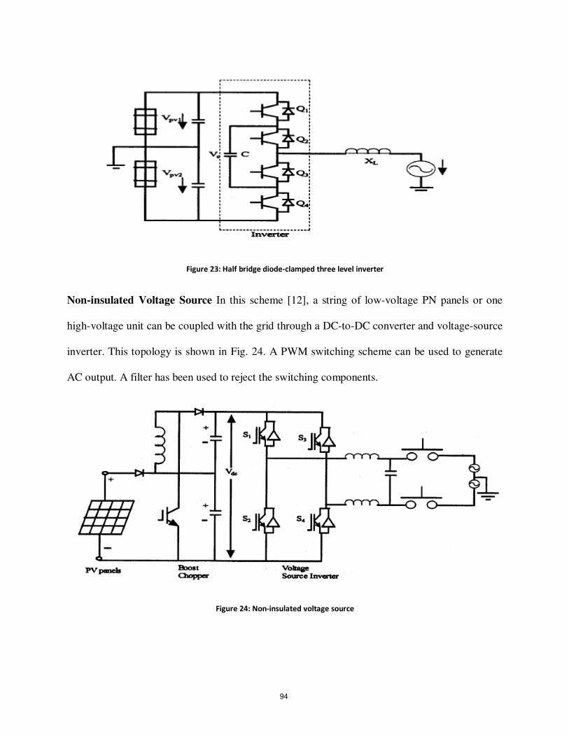
Figure 23: Half bridge diode-clamped three level inverter
Non-insulated Voltage Source In this scheme [12], a string of low-voltage PN panels or one
high-voltage unit can be coupled with the grid through a DC-to-DC converter and voltage-source
inverter. This topology is shown in Fig. 24. A PWM switching scheme can be used to generate
AC output. A filter has been used to reject the switching components.
Figure 24: Non-insulated voltage source
94
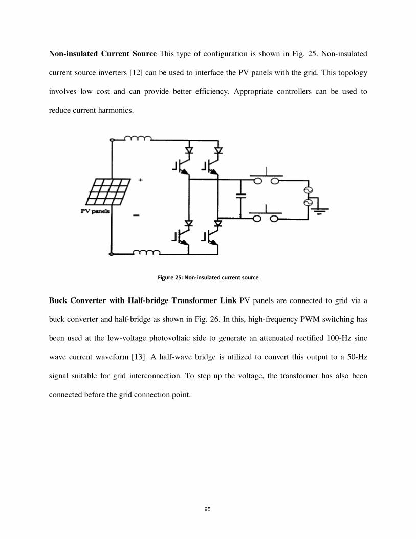
Non-insulated Current Source This type of configuration is shown in Fig. 25. Non-insulated
current source inverters [12] can be used to interface the PV panels with the grid. This topology
involves low cost and can provide better efficiency. Appropriate controllers can be used to
reduce current harmonics.
Figure 25: Non-insulated current source
Buck Converter with Half-bridge Transformer Link PV panels are connected to grid via a
buck converter and half-bridge as shown in Fig. 26. In this, high-frequency PWM switching has
been used at the low-voltage photovoltaic side to generate an attenuated rectified 100-Hz sine
wave current waveform [13]. A half-wave bridge is utilized to convert this output to a 50-Hz
signal suitable for grid interconnection. To step up the voltage, the transformer has also been
connected before the grid connection point.
95
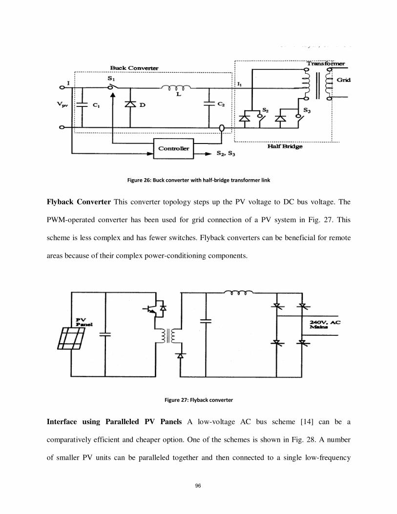
Figure 26: Buck converter with half-bridge transformer link
Flyback Converter This converter topology steps up the PV voltage to DC bus voltage. The
PWM-operated converter has been used for grid connection of a PV system in Fig. 27. This
scheme is less complex and has fewer switches. Flyback converters can be beneficial for remote
areas because of their complex power-conditioning components.
Figure 27: Flyback converter
Interface using Paralleled PV Panels A low-voltage AC bus scheme [14] can be a
comparatively efficient and cheaper option. One of the schemes is shown in Fig. 28. A number
of smaller PV units can be paralleled together and then connected to a single low-frequency
96
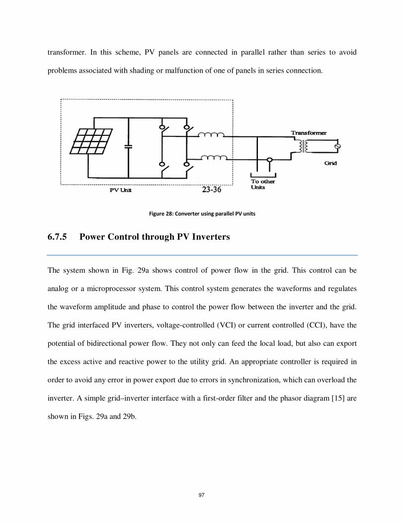
transformer. In this scheme, PV panels are connected in parallel rather than series to avoid
problems associated with shading or malfunction of one of panels in series connection.
Figure 28: Converter using parallel PV units
6.7.5 Power Control through PV Inverters
The system shown in Fig. 29a shows control of power flow in the grid. This control can be
analog or a microprocessor system. This control system generates the waveforms and regulates
the waveform amplitude and phase to control the power flow between the inverter and the grid.
The grid interfaced PV inverters, voltage-controlled (VCI) or current controlled (CCI), have the
potential of bidirectional power flow. They not only can feed the local load, but also can export
the excess active and reactive power to the utility grid. An appropriate controller is required in
order to avoid any error in power export due to errors in synchronization, which can overload the
inverter. A simple grid–inverter interface with a first-order filter and the phasor diagram [15] are
shown in Figs. 29a and 29b.
97
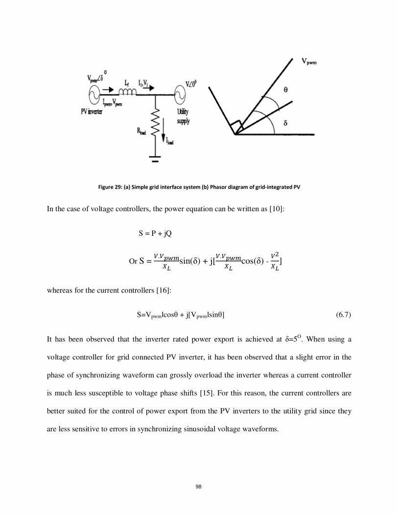
Figure 29: (a) Simple grid interface system (b) Phasor diagram of grid-integrated PV
In the case of voltage controllers, the power equation can be written as [10]:
S = P + jQ
Or S = .
sin(δ) + j[
.
cos(δ) -
]
whereas for the current controllers [16]:
S=Vpwmlcosθ + j[Vpwmlsinθ] (6.7)
It has been observed that the inverter rated power export is achieved at δ=5O. When using a
voltage controller for grid connected PV inverter, it has been observed that a slight error in the
phase of synchronizing waveform can grossly overload the inverter whereas a current controller
is much less susceptible to voltage phase shifts [15]. For this reason, the current controllers are
better suited for the control of power export from the PV inverters to the utility grid since they
are less sensitive to errors in synchronizing sinusoidal voltage waveforms.
98
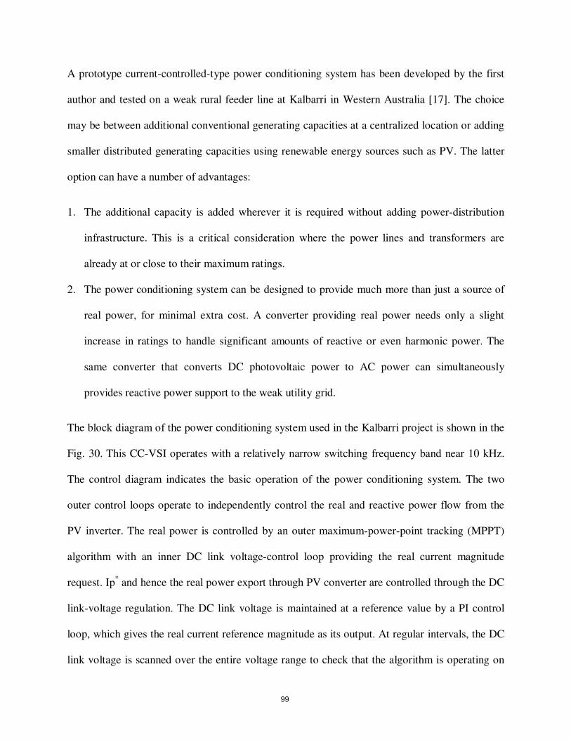
A prototype current-controlled-type power conditioning system has been developed by the first
author and tested on a weak rural feeder line at Kalbarri in Western Australia [17]. The choice
may be between additional conventional generating capacities at a centralized location or adding
smaller distributed generating capacities using renewable energy sources such as PV. The latter
option can have a number of advantages:
1. The additional capacity is added wherever it is required without adding power-distribution
infrastructure. This is a critical consideration where the power lines and transformers are
already at or close to their maximum ratings.
2. The power conditioning system can be designed to provide much more than just a source of
real power, for minimal extra cost. A converter providing real power needs only a slight
increase in ratings to handle significant amounts of reactive or even harmonic power. The
same converter that converts DC photovoltaic power to AC power can simultaneously
provides reactive power support to the weak utility grid.
The block diagram of the power conditioning system used in the Kalbarri project is shown in the
Fig. 30. This CC-VSI operates with a relatively narrow switching frequency band near 10 kHz.
The control diagram indicates the basic operation of the power conditioning system. The two
outer control loops operate to independently control the real and reactive power flow from the
PV inverter. The real power is controlled by an outer maximum-power-point tracking (MPPT)
algorithm with an inner DC link voltage-control loop providing the real current magnitude
request. Ip* and hence the real power export through PV converter are controlled through the DC
link-voltage regulation. The DC link voltage is maintained at a reference value by a PI control
loop, which gives the real current reference magnitude as its output. At regular intervals, the DC
link voltage is scanned over the entire voltage range to check that the algorithm is operating on
99
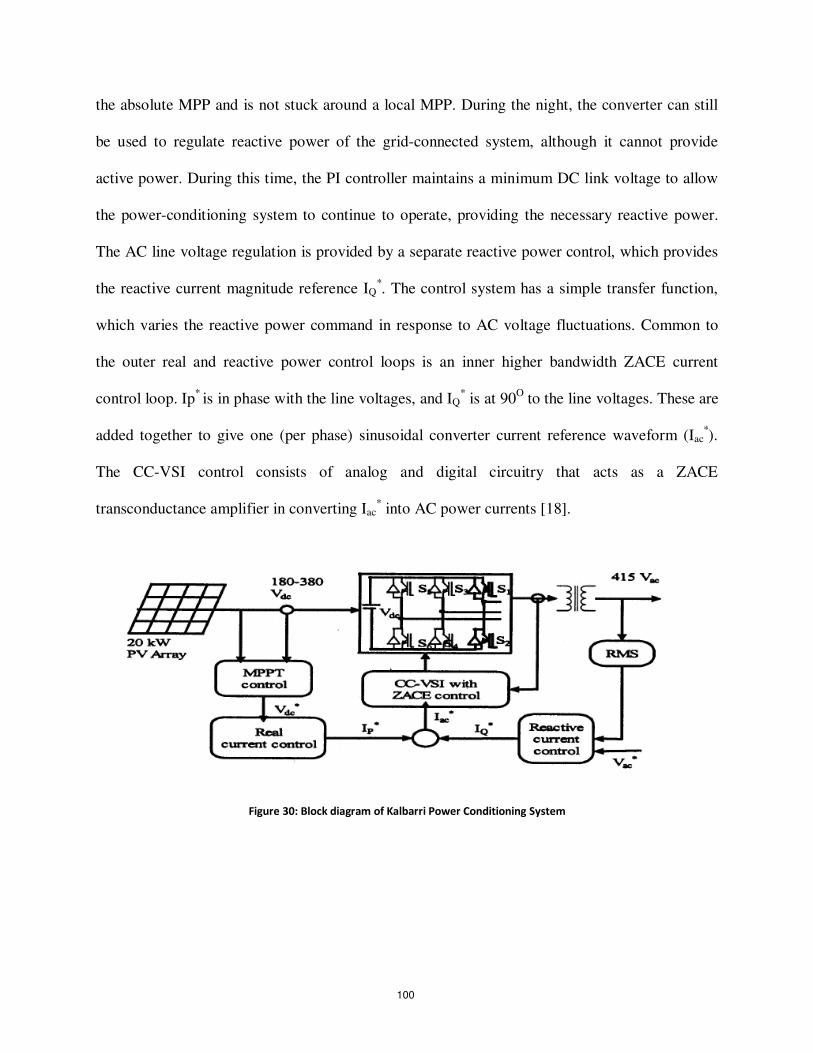
the absolute MPP and is not stuck around a local MPP. During the night, the converter can still
be used to regulate reactive power of the grid-connected system, although it cannot provide
active power. During this time, the PI controller maintains a minimum DC link voltage to allow
the power-conditioning system to continue to operate, providing the necessary reactive power.
The AC line voltage regulation is provided by a separate reactive power control, which provides
the reactive current magnitude reference IQ*. The control system has a simple transfer function,
which varies the reactive power command in response to AC voltage fluctuations. Common to
the outer real and reactive power control loops is an inner higher bandwidth ZACE current
control loop. Ip* is in phase with the line voltages, and IQ
* is at 90
O to the line voltages. These are
added together to give one (per phase) sinusoidal converter current reference waveform (Iac*).
The CC-VSI control consists of analog and digital circuitry that acts as a ZACE
transconductance amplifier in converting Iac* into AC power currents [18].
Figure 30: Block diagram of Kalbarri Power Conditioning System
100
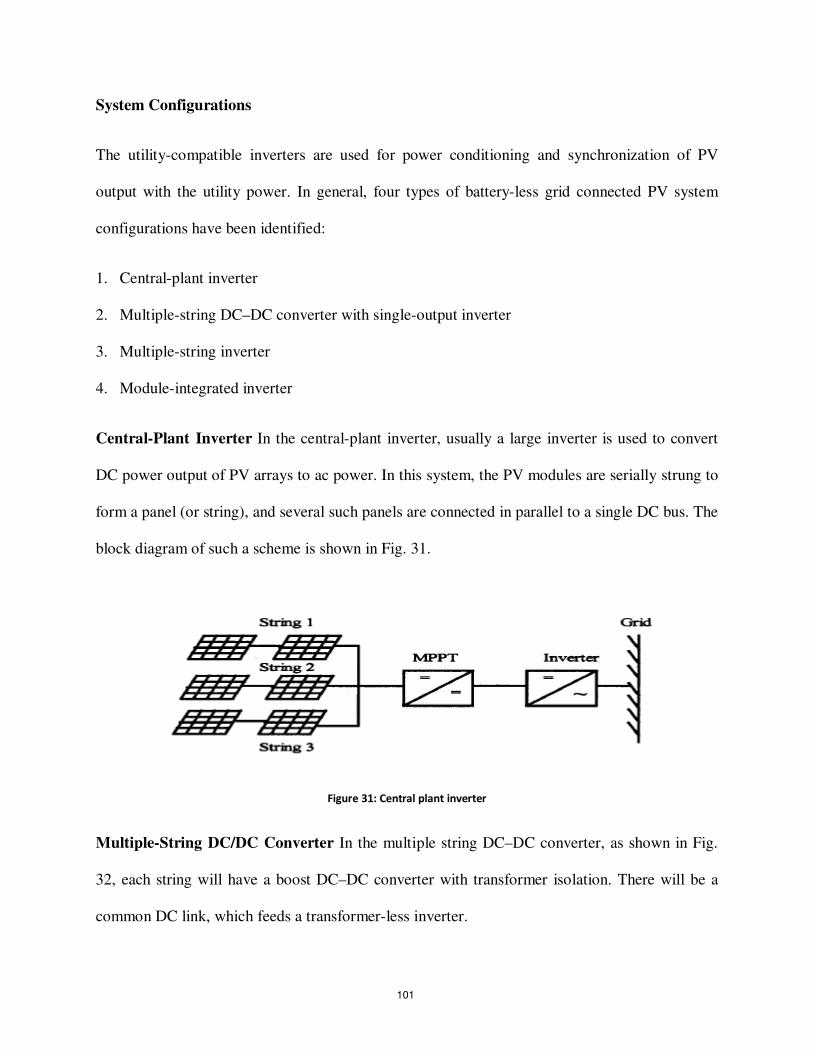
System Configurations
The utility-compatible inverters are used for power conditioning and synchronization of PV
output with the utility power. In general, four types of battery-less grid connected PV system
configurations have been identified:
1. Central-plant inverter
2. Multiple-string DC–DC converter with single-output inverter
3. Multiple-string inverter
4. Module-integrated inverter
Central-Plant Inverter In the central-plant inverter, usually a large inverter is used to convert
DC power output of PV arrays to ac power. In this system, the PV modules are serially strung to
form a panel (or string), and several such panels are connected in parallel to a single DC bus. The
block diagram of such a scheme is shown in Fig. 31.
Figure 31: Central plant inverter
Multiple-String DC/DC Converter In the multiple string DC–DC converter, as shown in Fig.
32, each string will have a boost DC–DC converter with transformer isolation. There will be a
common DC link, which feeds a transformer-less inverter.
101
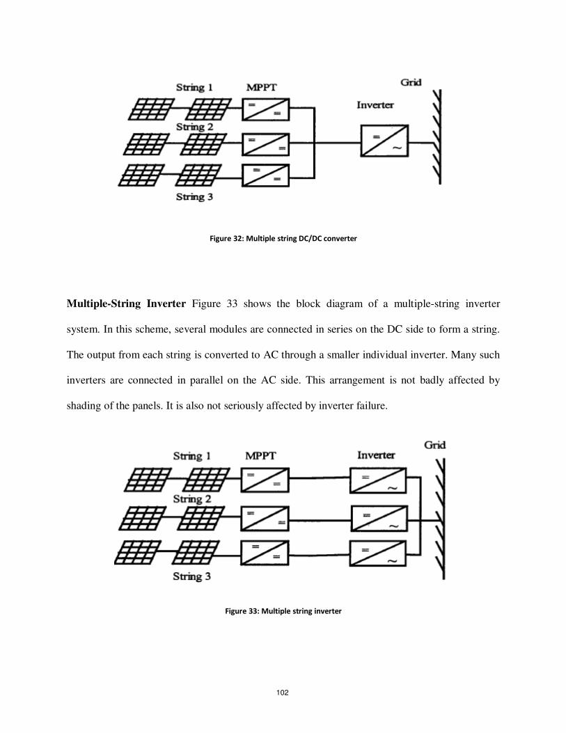
Figure 32: Multiple string DC/DC converter
Multiple-String Inverter Figure 33 shows the block diagram of a multiple-string inverter
system. In this scheme, several modules are connected in series on the DC side to form a string.
The output from each string is converted to AC through a smaller individual inverter. Many such
inverters are connected in parallel on the AC side. This arrangement is not badly affected by
shading of the panels. It is also not seriously affected by inverter failure.
Figure 33: Multiple string inverter
102

Module-Integrated Inverter In the module-integrated inverter system (Fig. 34), each module
(typically 50W to 300W) will have a small inverter. No cabling is required. It is expected that a
high volume of small inverters will bring down the cost.
Figure 34: Module integrated inverter
103
6.7.6 Grid-Compatible Inverter Characteristics
The characteristics of the grid-compatible inverters are:
1. Response time
2. Power factor
3. Frequency control
4. Harmonic output
5. Synchronization
6. Fault current contribution
7. DC current injection
8. Protection
The response time of the inverters must be extremely fast and governed by the bandwidth of the
control system. The absence of rotating mass and the use of semiconductor switches allow
inverters to respond in a millisecond time frame. The power factor of the inverters is traditionally
poor because of the displacement power factor and harmonics. But with the latest developments
in inverter technology, it is possible to maintain a power factor close to unity. The
converters/inverters have the capability of creating large voltage fluctuations by drawing reactive
power from the utility rather than supplying it [19]. With proper control, inverters can provide
voltage support by importing/exporting reactive power to push/pull toward a desired set point.
This function would be of more use to the utilities as it can assist in the regulation of the grid
system at the domestic consumer level.
The frequency of the inverter output wave-shape is locked to the grid. Frequency bias is where
the inverter frequency is deliberately made to run at, say, 53 Hz. When the grid is present, this
104
will be pulled down to the nominal 50 Hz. If the grid fails, it will drift upward toward 53Hz and
trip on over-frequency. This can help in preventing islanding.
Harmonic output from inverters has traditionally been very poor. Old thyristor-based inverters
operated with slow switching speeds and could not be pulse-width modulated. This resulted in
inverters known as six-pulse or 12-pulse inverters. The harmonics so produced from the inverters
can be injected into the grid, resulting in losses, heating of appliances, tripping of protection
equipment, and poor power quality, the number of pulses being the number of steps in a sine-
wave cycle. With the present advances in power-electronics technology, inverter controls can be
made very good. PWM inverters produce high-quality sine waves. The harmonic levels are very
low and can be lower than those of common domestic appliances. If harmonics are present in the
grid voltage waveform, harmonic currents can be induced in the inverter. These harmonic
currents, particularly those generated by a voltage-controlled inverter, will in fact help in
supporting the grid. These are good harmonic currents. This is the reason that the harmonic
current output of inverters must be measured onto a clean grid source so that only the harmonics
being produced by the inverters are measured.
Synchronization of inverters with the grid is performed automatically and typically uses zero-
crossing detection on the voltage waveform. An inverter has no rotating mass and hence has no
inertia. Synchronization does not involve the acceleration of a rotating machine. Consequently,
the reference waveforms in the inverter can be jumped to any point required within a sampling
period. If phase-locked loops are used, the jump could take up a few seconds. Phase-locked loops
are used to increase the immunity to noise. This allows the synchronization to be based on
several cycles of zero-crossing information. The response time for this type of locking will be
slower.
105
PV panels produce a current that is proportional to the amount of light falling on them. The
panels are normally rated to produce 1000W/m2 at 25
OC. Under these conditions, the short
circuit current possible from these panels is typically only 20% higher than the nominal current,
whereas it is extremely variable for wind. If the solar radiation is low then the maximum current
possible under short circuit is going to be less than the nominal full-load current. Consequently,
PV systems cannot provide short-circuit capacity to the grid. If a battery is present, the fault
current contribution is limited by the inverter. With battery storage, it is possible for the battery
to provide the energy. However, inverters are typically limited to between 100% and 200% of
nominal rating under current-limit conditions. The inverter needs to protect itself against short
circuits because the power electronic components will typically be destroyed before a protection
device such as a circuit breaker trip. In case of inverter malfunction, inverters have the capability
to inject the DC components into the grid. Most utilities have guidelines for this purpose. A
transformer must be installed at the point of connection on the AC side to prevent DC from
entering the utility network. The transformer can be omitted when a DC detection device is
installed at the point of connection on the AC side in the inverter. The DC injection is essentially
caused by the reference or power electronics device producing a positive half-cycle that is
different from the negative half-cycle resulting into the DC component in the output. If the DC
component can be measured, it can then be added into the feedback path to eliminate the DC
quantity.
106
6.8 Protection Requirements
A minimum requirement to facilitate the prevention of islanding is that the inverter energy
system protection operates and isolates the inverter energy system from the grid if any of the
following occurs:
1. Overvoltage
2. Under-voltage
3. Over-frequency
4. Under-frequency
These limits may be either factory-set or site-programmable. The protection voltage operating
points may be set in a narrower band if required, e.g., 220 V to 260 V. In addition to the passive
protection detailed above, and to prevent the situation where islanding may occur because
multiple inverters provide a frequency reference for one another, inverters must have an accepted
active method of islanding prevention following grid failure, e.g., frequency drift or impedance
measurement. Inverter controls for islanding can be designed on the basis of detection of grid
voltage, measurement of impedance, frequency variation, or increase in harmonics. This function
must operate to force the inverter output outside the protection tolerances specified previously,
thereby resulting in isolation of the inverter energy system from the grid. The maximum
combined operation time of both passive and active protections should be 2 seconds after grid
failure under all local load conditions. If frequency shift is used, it is recommended that the
direction of shift be down. The inverter energy system must remain disconnected from the grid
until the reconnection conditions are met. Some inverters produce high-voltage spikes, especially
107

at light load, which can be dangerous for the electronic equipment. IEEE P929 gives some idea
of the permitted voltage limits.
If the inverter energy system does not have the preceding frequency features, the inverter must
incorporate an alternate anti-islanding protection feature that is acceptable to the relevant
electricity distributor. If the protection function above is to be incorporated in the inverter, it
must be type tested for compliance with these requirements and accepted by the relevant
electricity distributor. Otherwise, other forms of external protection relaying are required that
have been type tested for compliance with these requirements and approved by the relevant
electricity distributor. The inverter must have adequate protection against short-circuit, other
faults, and overheating of inverter components.
108
109
Chapter 7
Solar photovoltaics
Introduction:
The photovoltaic (pv) power technology uses semiconductor cells (wafers), generally several square
centimeters in size. From the solid-state physics point of view, the cell is basically a large area p-n diode
with the junction positioned close to the top surface. The cell converts the sunlight into direct current
electricity. Numerous cells are assembled in a module to generate required power. Unlike the dynamic
wind turbine, the pv installation is static, does not need strong tall towers, produces no vibration or noise,
and needs no cooling. Because much of the current pv technology uses crystalline semiconductor material
similar to integrated circuit chips, the production costs have been high. However, between 1980 and 1996,
the capital cost of pv modules per watt of power capacity has declined.
Solar photovoltaics (SPV):
Solar photovoltaic (SPV) is the process of converting solar radiation into electricity using a device called
solar cell. A solar cell is a semi-conducting device made of silicon or other materials, which, when
exposed to sunlight, generates electricity.
Factors affecting magnitude of electric current:
1. Intensity of the solar radiation
2. Exposed area of the solar cell
3. Type of material used in fabricating the solar cell
4. Ambient temperature
Hierarchical arrangement:
A hierarchical arrangement of components of PV system is shown in Figure 1.
110
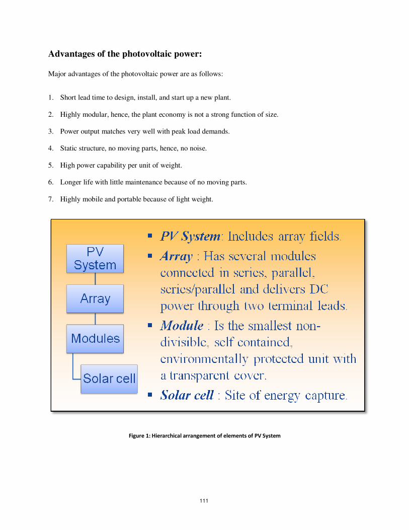
Advantages of the photovoltaic power:
Major advantages of the photovoltaic power are as follows:
1. Short lead time to design, install, and start up a new plant.
2. Highly modular, hence, the plant economy is not a strong function of size.
3. Power output matches very well with peak load demands.
4. Static structure, no moving parts, hence, no noise.
5. High power capability per unit of weight.
6. Longer life with little maintenance because of no moving parts.
7. Highly mobile and portable because of light weight.
Figure 1: Hierarchical arrangement of elements of PV System
111
Solar photovoltaic in India:
India is implementing perhaps the most number of pv systems in the world for remote villages. About 30
MW capacity has already been installed, with more being added every year. The country has a total
production capacity of 8.5 MW modules per year. The remaining need is met by imports. A 700 kW grid-
connected PV plant has been commissioned, and a 425 kW capacity is under installation in Madhya
Pradesh. The state of West Bengal has decided to convert the Sagar Island into a PV island. The island
has 150,000 inhabitants in 16 villages spread out in an area of about 300 square kilometers. The main
source of electricity at present is diesel, which is expensive and is causing severe environmental problems
on the island.
The state of Rajasthan has initialed a policy to purchase PV electricity at an attractive rate of $0.08 per
kWh. In response, a consortium of Enron and Amoco has proposed installing a 50 MW plant using thin
film cells. When completed, this will be the largest PV power plant in the world. The studies at the Arid
Zone Research Institute, Jodhpur, indicate significant solar energy reaching the earth surface in India.
About 30 percent of the electrical energy used in India is for agricultural needs. Since the availability of
solar power for agricultural need is not time critical (within a few days), India is expected to lead the
world in PV installations in near future.
Interesting fact:
One of the attractive features of the pv system is that its power output matches very well with the peak
load demand. It produces more power on a sunny summer day when the air-conditioning load strains the
grid lines. Power usage curve in commercial building on a typical summer day is shown in Figure 2.
112
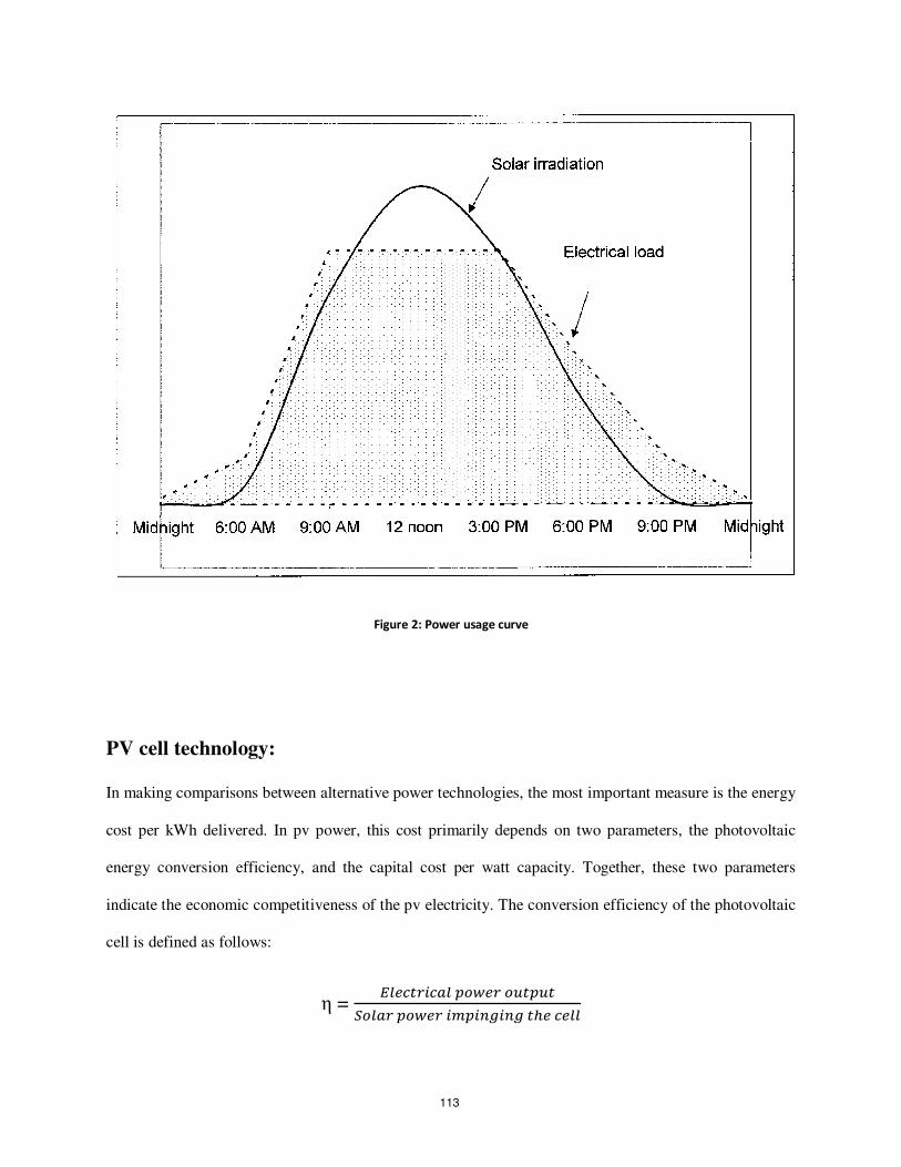
Figure 2: Power usage curve
PV cell technology:
In making comparisons between alternative power technologies, the most important measure is the energy
cost per kWh delivered. In pv power, this cost primarily depends on two parameters, the photovoltaic
energy conversion efficiency, and the capital cost per watt capacity. Together, these two parameters
indicate the economic competitiveness of the pv electricity. The conversion efficiency of the photovoltaic
cell is defined as follows:
η =
113
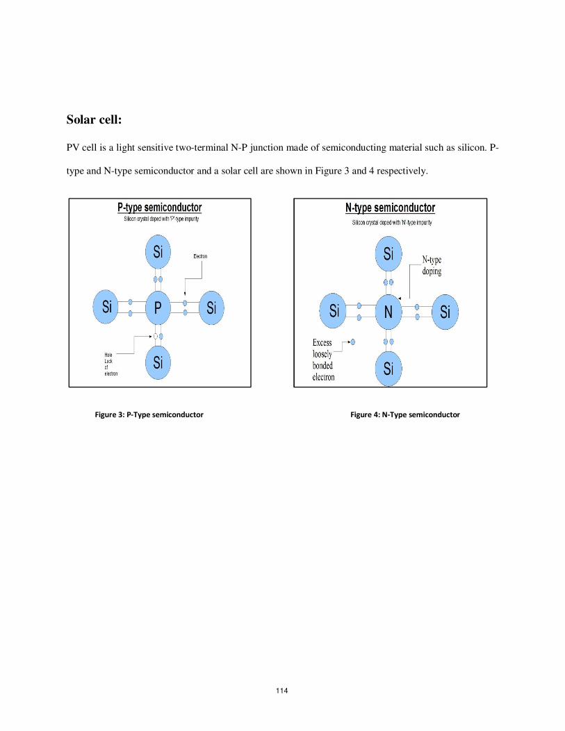
Solar cell:
PV cell is a light sensitive two-terminal N-P junction made of semiconducting material such as silicon. P-
type and N-type semiconductor and a solar cell are shown in Figure 3 and 4 respectively.
Figure 3: P-Type semiconductor Figure 4: N-Type semiconductor
114
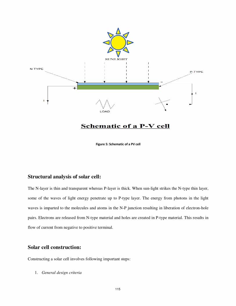
Figure 5: Schematic of a PV cell
Structural analysis of solar cell:
The N-layer is thin and transparent whereas P-layer is thick. When sun-light strikes the N-type thin layer,
some of the waves of light energy penetrate up to P-type layer. The energy from photons in the light
waves is imparted to the molecules and atoms in the N-P junction resulting in liberation of electron-hole
pairs. Electrons are released from N-type material and holes are created in P-type material. This results in
flow of current from negative to positive terminal.
Solar cell construction:
Constructing a solar cell involves following important steps:
1. General design criteria
115
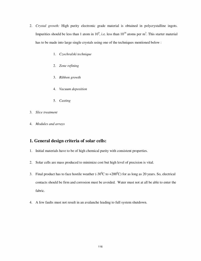
2. Crystal growth: High purity electronic grade material is obtained in polycrystalline ingots.
Impurities should be less than 1 atom in 109, i.e. less than 1018 atoms per m3. This starter material
has to be made into large single crystals using one of the techniques mentioned below :
1. Czochralski technique
2. Zone refining
3. Ribbon growth
4. Vacuum deposition
5. Casting
3. Slice treatment
4. Modules and arrays
1. General design criteria of solar cells:
1. Initial materials have to be of high chemical purity with consistent properties.
2. Solar cells are mass produced to minimize cost but high level of precision is vital.
3. Final product has to face hostile weather (-300C to +2000C) for as long as 20 years. So, electrical
contacts should be firm and corrosion must be avoided. Water must not at all be able to enter the
fabric.
4. A few faults must not result in an avalanche leading to full system shutdown.
116
2. Crystal growth:
Czochralski technique: Czochralski technique of developing crystals of solar cell is explained below:
1. Dip a small seed crystal into molten material.
2. Add dopant (boron acceptors for p type) to melt and pull crystal mechanically upward with a 15
cm dia. crystal growing from the seed.
3. Slice crystal 300 µm thick with highly accurate diamond saws.
Zone refining technique: Zone refining technique of developing crystals of solar cell is explained below:
1. Polycrystalline material is formed as a rod.
2. Molten zone is passed along the rod by heating with a radio frequency coil or lasers.
3. Purified material forms single crystal which is then sliced and treated.
3. Slice treatment:
1. The 300-400 µm thick slices are chemically etched.
2. A very thin layer of N type material is formed by diffusion of donors (e.g. phosphorus) for the top
surface by heating the slices to 10000C in atmosphere of N2 in presence of POCL3.
3. Photolithographic methods: (Si-Ti-Pd-Ag)
1. On Si surface, Ti is deposited to form a low resistance contact.
2. Then thin Pd layer is placed to prevent chemical reaction of Ti with Ag.
117
3. Finally Ag is deposited for current carrying grid.
4. Modules and arrays:
Individual cells of size 10 x 10 cm are connected into modules of 30 cells. Module consists of 3 to 5
columns of cells in series producing an EMF of 15V which is safe and convenient for charging 12V
batteries. Now, a SPV becomes ready for installation at site.
Power of a Solar Panel, Array and Module:
Let n = Number of solar cells in a module;
m= Number of modules in an array or a panel;
Pc=Power per solar cell, watts
Therefore, power per module = n x Pc
Power per array or panel = m x n x Pc
Pp = m x n x Pc ….. W
For full light, solar panel will deliver power Pp.
Standards for SPV:
1) Bureau of Indian Standards (BIS) establishes the photovoltaic standards in India.
2) Standards specified by BIS for SPV in India relate to areas listed below:
1. SPV terminology
2. Measurements of cells and modules
118
3. Methods of correcting the measurements
4. Qualification test procedure for crystalline silicon modules
5. General description of SPV power generating systems
6. Parameters of stand-alone SPV systems
Standard capacity/ratings and specifications:
1) The wattage output of a PV module is rated in terms of peak watt (Wp) units.
2) The peak watt output that the module could deliver under standard test conditions (STC).
3) STC conditions:
i) 1000 watts per square meter solar radiation intensity
ii) Air-mass 1.5 reference spectral distribution
iii) 250C ambient temperature.
4) SPV systems in India are of range 5Wp-120Wp.
Testing and certification of SPV:
The ministry of Non-Conventional Energy Sources (MNES) has established facilities for testing of testing
of solar cells, PV modules, and systems at its Solar Energy Center (SEC) in Gurgaon, Haryana.
Other test centers are Electronic Testing and Development Laboratory (ETDC), Bangalore, Electronic
Regional Testing Laboratory (ERTL-East), Kolkata and Central Power Research Institute (CPRI),
Thiruvananthapuram.
119
India has currently about 14 companies that manufacture PV modules, and over 45 companies that
manufacture SPV systems.
Limits to cell efficiency:
Various factors limit the efficiency of a solar cell. They are mentioned below:
(N.B.: Detailed description of factors mentioned below is provided in Appendix.)
1. Top surface contact obstruction ( loss ~3%)
2. Reflection at top surface ( loss ~1%)
3. Photon energy less than band gap (loss ~23%)
4. Excess photon energy (loss ~33%)
5. Quantum efficiency (loss ~0.4%)
6. Collection efficiency
7. Voltage factor FV (loss ~20%)
8. Curve factor FC (loss ~4%)
9. Additional curve factor A (loss ~5%)
10. Series resistance (loss ~0.3%)
11. Shunt resistance (negligible, ~0.1%)
12. Delivered power (Si cell 10 to 14%)
120
Experiments in Photovoltaics
Experiment 1
Aim of the Experiment:
This experiment is done to calibrate a solar photovoltaic array and determine its characteristic curve.
Also, determine solar radiation intensity at NIT Rourkela.
Appratus Required:
Sl.
No.
Name of the
equipment
Specifications Quantity
1 Solar Module Consisting of 36 solar cells consisting of 4 rows X 9
columns
1
2 Ammeter 0-5A (MC) 1
3 Voltmeter 0-75 V (MI) 1
4 CRO Dual Trace 1
5 Rheostat 300 Ohm, 1.2A 1
6 Connecting Wires As required
Experimental Setup and Procedure:
The solar panel at our Electrical Machines laboratory consists of 36 solar cells of about 10 cm diameters
each. When direct sunlight falls on this panel, a direct current flows through the entire circuit. Suitable
arrangement was made to detect the waveform of the generated current and study its components. The
121
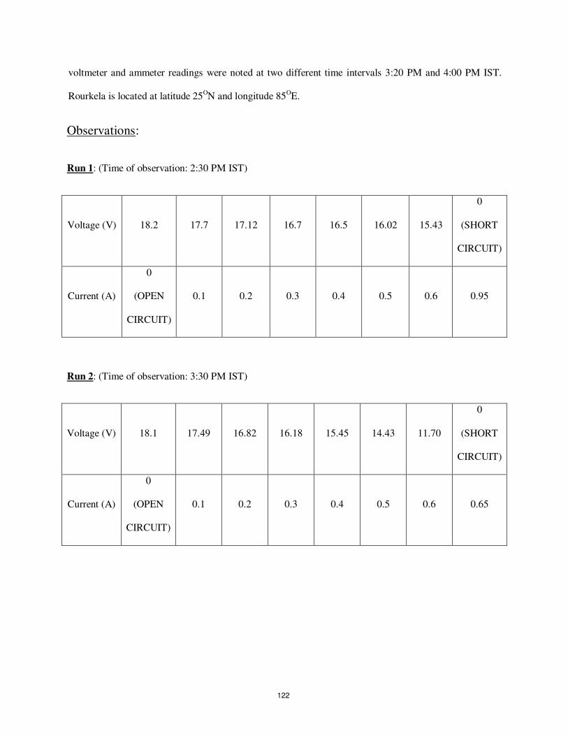
voltmeter and ammeter readings were noted at two different time intervals 3:20 PM and 4:00 PM IST.
Rourkela is located at latitude 25ON and longitude 85OE.
Observations:
Run 1: (Time of observation: 2:30 PM IST)
Voltage (V) 18.2 17.7 17.12 16.7 16.5 16.02 15.43
0
(SHORT
CIRCUIT)
Current (A)
0
(OPEN
CIRCUIT)
0.1 0.2 0.3 0.4 0.5 0.6 0.95
Run 2: (Time of observation: 3:30 PM IST)
Voltage (V) 18.1 17.49 16.82 16.18 15.45 14.43 11.70
0
(SHORT
CIRCUIT)
Current (A)
0
(OPEN
CIRCUIT)
0.1 0.2 0.3 0.4 0.5 0.6 0.65
122
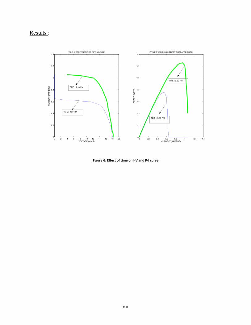
Results :
Figure 6: Effect of time on I-V and P-I curve
0 2 4 6 8 10 12 14 16 18 200
0.2
0.4
0.6
0.8
1
1.2
1.4
VOLTAGE (VOLT)
CU
RR
EN
T (
AM
PE
RE
)
V-I CHARACTERISTIC OF SPV MODULE
0 0.2 0.4 0.6 0.8 1 1.2 1.40
2
4
6
8
10
12
14
CURRENT (AMPERE)
PO
WE
R (
WA
TT
)
POWER VERSUS CURRENT CHARACTERISTIC
TIME : 2.30 PM
TIME : 3.30 PM
TIME : 2.30 PM
TIME : 3.30 PM
123
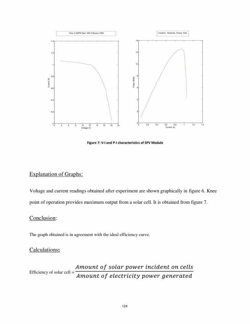
Figure 7: V-I and P-I characteristics of SPV Module
Explanation of Graphs:
Voltage and current readings obtained after experiment are shown graphically in figure 6. Knee
point of operation provides maximum output from a solar cell. It is obtained from figure 7.
Conclusion:
The graph obtained is in agreement with the ideal efficiency curve.
Calculations:
Efficiency of solar cell =
2 4 6 8 10 12 14 16 18 200
0.2
0.4
0.6
0.8
1
1.2
1.4
Voltage (V)
Cu
rre
nt
(A)
0 0.2 0.4 0.6 0.8 1 1.2 1.40
2
4
6
8
10
12
14
Current (A)
Po
we
r (W
att
)
Location : Rourkela, Orissa, IndiaTime: 2.30PM Date: 20th February 2009
124
Let n = Number of solar cells in a module;
m= Number of modules in an array or a panel;
Pc=Power per solar cell, watts
Power per module = n x Pc
Power per array or panel = m x n x Pc
Pp = m x n x Pc ….. W
For full light, solar panel will deliver power Pp.
At NIT Rourkela, amount of electricity produced = 10% of incident energy
Also, diameter of a solar cell = 10 cm
Area of 1 PV cell =
D2 = 78.57 cm2
No. of PV cells in array = 4 (columns) X 9 (rows) i.e. m=4, n=9
Total exposed area of cells = 36 X 78.57 = 0.283 m2
Radiation Intensity =P !"#
A! = 864 W/m2
125
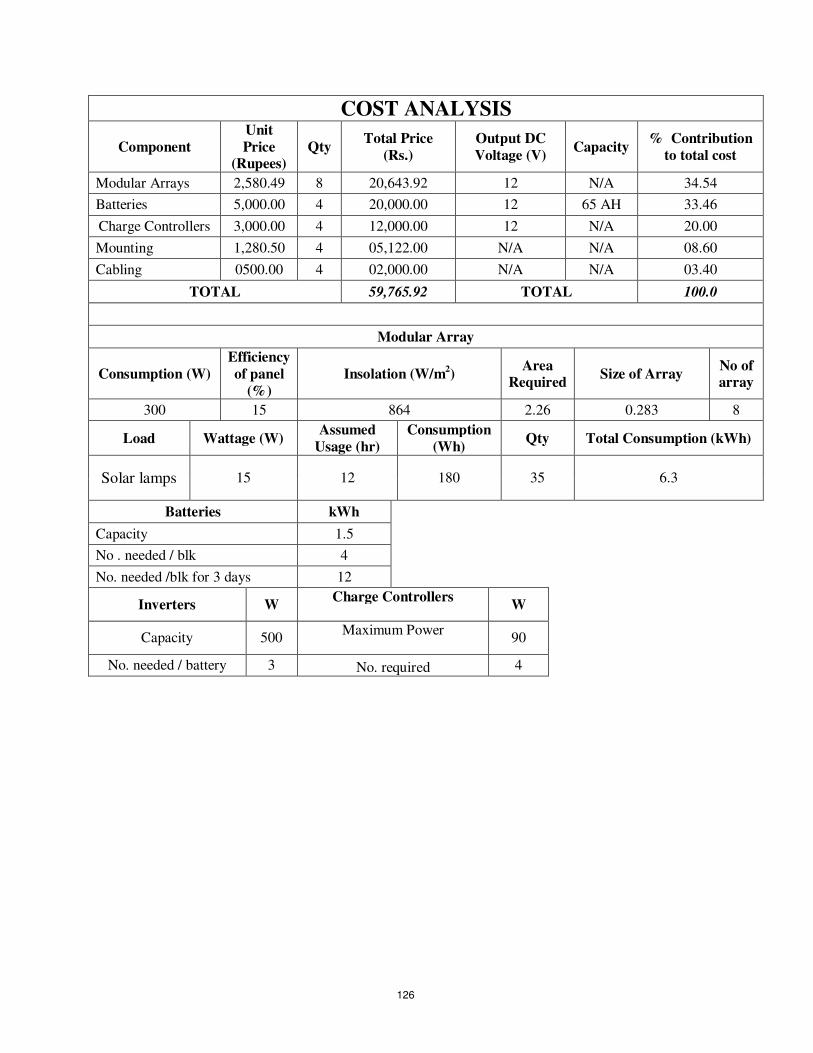
COST ANALYSIS
Component
Unit
Price
(Rupees)
Qty Total Price
(Rs.)
Output DC
Voltage (V) Capacity
% Contribution
to total cost
Modular Arrays 2,580.49 8 20,643.92 12 N/A 34.54
Batteries 5,000.00 4 20,000.00 12 65 AH 33.46
Charge Controllers 3,000.00 4 12,000.00 12 N/A 20.00
Mounting 1,280.50 4 05,122.00 N/A N/A 08.60
Cabling 0500.00 4 02,000.00 N/A N/A 03.40
TOTAL 59,765.92 TOTAL 100.0
Modular Array
Consumption (W)
Efficiency
of panel
(%)
Insolation (W/m2)
Area
Required Size of Array
No of
array
300 15 864 2.26 0.283 8
Load Wattage (W) Assumed
Usage (hr)
Consumption
(Wh) Qty Total Consumption (kWh)
Solar lamps 15 12 180 35 6.3
Batteries kWh
Capacity 1.5
No . needed / blk 4
No. needed /blk for 3 days 12
Inverters W Charge Controllers
W
Capacity 500 Maximum Power
90
No. needed / battery 3 No. required 4
126
Experiment 2
Aim of the experiment:
Voltage analysis of a load receiving power from a nearby solar photovoltaic power module.
Theory:
The duty cycle is the fraction of time during which the switch is on. For control purposes the
pulse width can be adjusted to achieve a desired result. This adjustment process is called pulse-
width modulation (PWM), perhaps the most important process for implementing control in
power converters.
Frequency is mostly constant and is often dictated by the application.
PWM inverters produce high-quality sine waves. The harmonic levels are very low and can be
lower than those of common domestic appliances.
PWM techniques: In single PWM, there is only one pulse per half-cycle and the width of the
pulse is varied to control the inverter output voltage.
In sinusoidal modulation, the width of each pulse is varied in proportion to the amplitude of a
sine wave evaluated at the center of the same pulse.
127

Appratus Required:
Sl. No. Name of the equipment Specifications Quantity
1 Solar Module Consisting of 36 solar cells (4 rows X 9 columns) 1
2 Ammeter 0-5A (MC) 1
3 Voltmeter 0-75 V (MI) 1
4 CRO Storage type 1
5 Rheostat 50 Ohm, 1.2A 1
6 Inductor 50 mH,100 mH,250 mH 3
7 Interfacing cord For connecting CRO to desktop 1
8 TekVision Software Installed on desktop -
6 Connecting Wires As required
Figure 6: EXPERIMENTAL SETUP
128
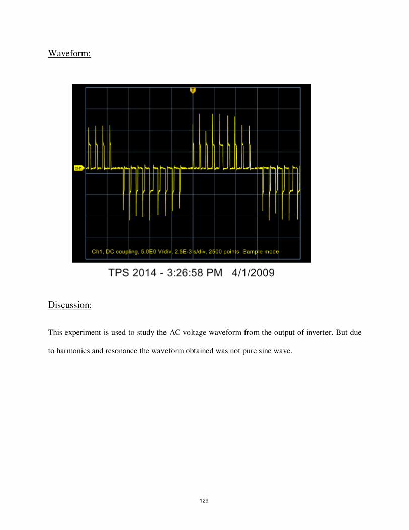
Waveform:
Discussion:
This experiment is used to study the AC voltage waveform from the output of inverter. But due
to harmonics and resonance the waveform obtained was not pure sine wave.
129
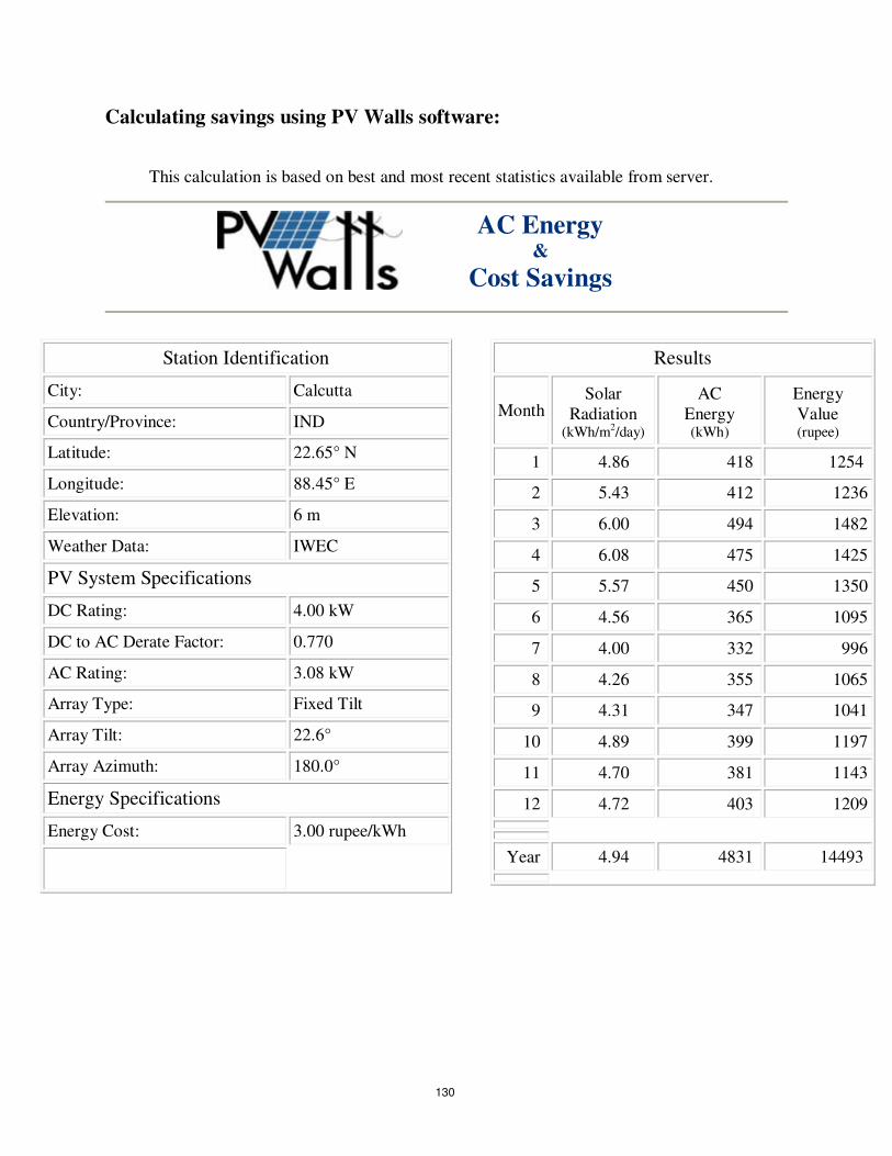
Calculating savings using PV Walls software:
This calculation is based on best and most recent statistics available from server.
* * * * *
AC Energy
&
Cost Savings
* * * * *
Station Identification
City: Calcutta
Country/Province: IND
Latitude: 22.65° N
Longitude: 88.45° E
Elevation: 6 m
Weather Data: IWEC
PV System Specifications
DC Rating: 4.00 kW
DC to AC Derate Factor: 0.770
AC Rating: 3.08 kW
Array Type: Fixed Tilt
Array Tilt: 22.6°
Array Azimuth: 180.0°
Energy Specifications
Energy Cost: 3.00 rupee/kWh
Results
Month
Solar Radiation
(kWh/m2/day)
AC Energy (kWh)
Energy Value (rupee)
1 4.86 418 1254
2 5.43 412 1236
3 6.00 494 1482
4 6.08 475 1425
5 5.57 450 1350
6 4.56 365 1095
7 4.00 332 996
8 4.26 355 1065
9 4.31 347 1041
10 4.89 399 1197
11 4.70 381 1143
12 4.72 403 1209
Year 4.94 4831 14493
130
Chapter 8
PEM Fuel Cell
131

POLYMER ELECTROLYTE MEMBRANE FUEL CELLS
Polymer electrolyte membrane fuel cells (PEFC) are able to efficiently generate high power
densities, thereby making the technology potentially attractive for certain mobile and portable
applications. Especially the possible application of PEFC as a prime mover for automobiles has
captured the imagination of many. PEFC technology differentiates itself from other fuel cell
technologies in that a solid phase polymer membrane is used as the cell separator/electrolyte.
Because the cell separator is a polymer film and the cell operates at relatively low temperatures,
issues such as sealing, assembly, and handling are less complex than most other fuel cells. The
need to handle corrosive acids or bases is eliminated in this system. PEFCs typically operate at
low temperatures (60O
to 80OC), allowing for potentially faster startup than higher temperature
fuel cells. The PEFC is seen as the main fuel cell candidate technology for light-duty
transportation applications. While PEFC are particularly suitable for operation on pure hydrogen,
fuel processors have been developed that will allow the use of conventional fuels such as natural
gas or gasoline. A unique implementation of the PEFC allows the direct use of methanol without
a fuel processor; it is the direct methanol fuel cell (DMFC). The DMFC is seen as the leading
candidate technology for the application of fuel cells to cameras, notebook computers, and other
portable electronic applications.
132

8.1 Cell Components
Typical cell components within a PEFC stack include:
• the ion exchange membrane
• an electrically conductive porous backing layer
• an electro-catalyst (the electrodes) at the interface between the backing layer and the
membrane
• cell interconnects and flow-plates that deliver the fuel and oxidant to reactive sites via
flow channels and electrically connect the cells (Figure 1 & 2).
PEFC stacks are almost universally of the planar bipolar type. Typically, the electrodes are cast
as thin films that are either transferred to the membrane or applied directly to the membrane.
Alternatively, the catalyst-electrode layer may be deposited onto the backing layer, then bonded
to the membrane.
133
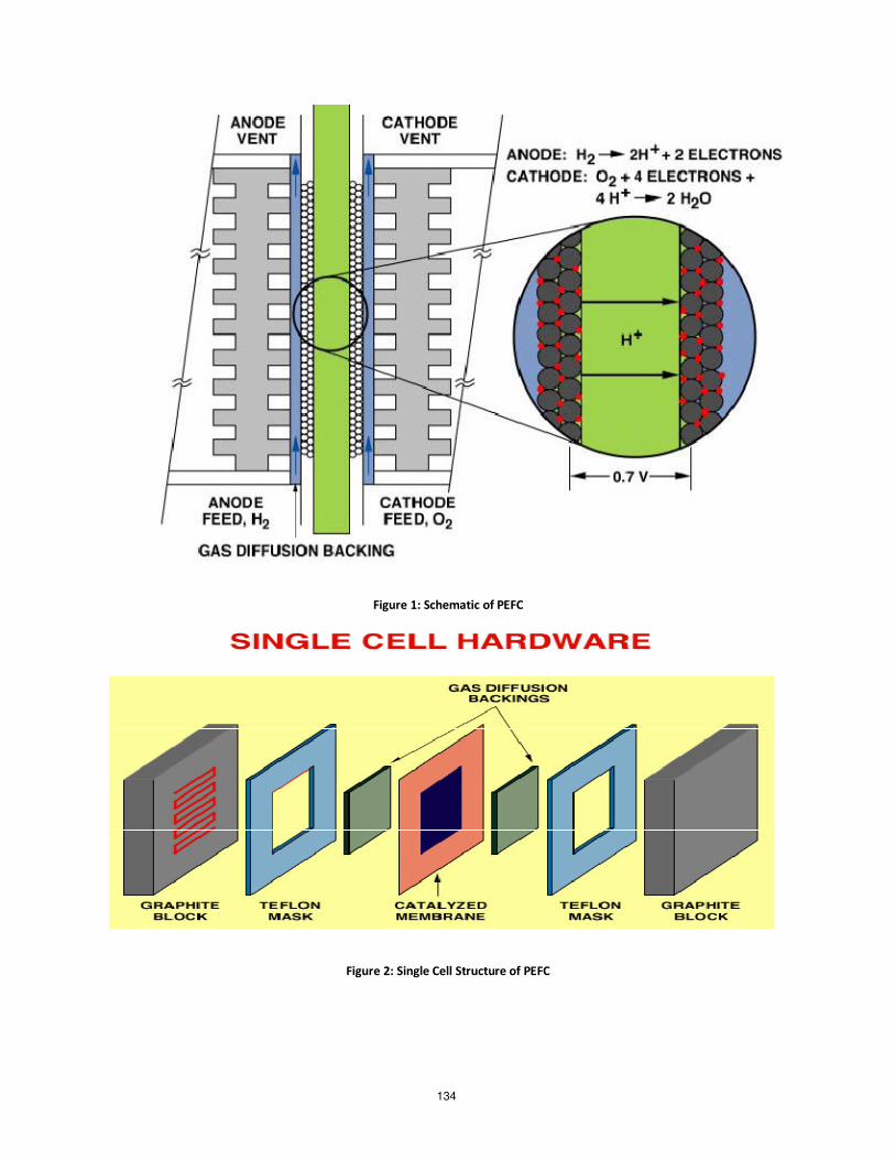
Figure 1: Schematic of PEFC
Figure 2: Single Cell Structure of PEFC
134

8.1.1 Membrane
Organic-based cation exchange membranes in fuel cells were originally conceived by William T.
Grubb (2) in 1959. That initial effort eventually led to development of the perfluorosulfonic acid
polymer used in today’s systems. The function of the ion exchange membrane is to provide a
conductive path, while at the same time separating the reactant gases. The material is an
electrical insulator. As a result, ion conduction takes place via ionic groups within the polymer
structure. Ion transport at such sites is highly dependent on the bound and free water associated
with those sites. An accelerated interest in polymer electrolyte fuel cells has led to improvements
in both cost and performance. Development has reached the point where both motive and
stationary power applications are nearing an acceptable cost for commercial markets. Operation
of PEFC membrane electrode assemblies (MEAs) and single cells under laboratory conditions
similar to transportation or stationary applications have operated for over 20,000 hrs
continuously with degradation rates of 4 to 6 V/hr (or about 0.67 to 1.0 percent per 1000 hrs),
which approaches the degradation rates needed for stationary applications (about 0.1 percent per
1000 hrs is used as a rule of thumb). Complete fuel cell systems have been demonstrated for a
number of transportation applications including public transit buses and passenger automobiles.
For stationary applications, a number of demonstration systems have been developed and
numerous systems have been installed, mostly in the 2 to 10 kW range. However, although these
systems have collectively logged millions of kWhrs (3), developers have not yet demonstrated
system or stack life of more than 8,000 hours with realistic catalyst loadings and realistic
operating conditions, and then with degradation rates of several percent per 1000 hrs.
Consequently, PEFC developers and researchers are focused on achieving critical improvements
135
in extending stack life, simpler system integration, and reduction of system cost. This is true both
for stationary and mobile applications.
8.1.2 Porous Backing Layer
The polymer membrane is sandwiched between two sheets of porous backing media (also
referred to as gas diffusion layers or current collectors). The functions of the backing layer8 are
to:
(1) act as a gas diffuser;
(2) provide mechanical support,
(3) provide an electrical pathway for electrons, and
(4) channel product water away from the electrodes.
The backing layer is typically carbon-based, and may be in cloth form, a non-woven pressed
carbon fiber configuration, or simply a felt-like material. The layer incorporates a hydrophobic
material, such as polytetrafluoroethylene. The function of polytetrafluoroethylene is to prevent
water from “pooling” within the pore volume of the backing layer so that gases freely contact the
catalyst sites. Furthermore, it facilitates product water removal on the cathode as it creates a non-
wetting surface within the passages of the backing material.
One PEFC developer (10) devised an alternative plate structure that provides passive water
control. Product water is removed by two mechanisms:
(1) transport of liquid water through the porous bipolar plate into the coolant, and
(2) evaporation into the reactant gas streams.
136

The cell is similar in basic design to other PEFCs with membrane, catalysts, substrates, and
bipolar plate components. However, there is a difference in construction and composition of the
bipolar plate: it is made of porous graphite. During operation, the pores are filled with liquid
water that communicates directly with the coolant stream. Product water flows from the cathode
through the pores into the coolant stream (a small pressure gradient between reactant and the
coolant stream is needed). The water in the coolant stream is then routed to a reservoir. Removal
of water by the porous membrane results in the reactant flow stream being free of any
obstructions (liquid water). The flooded pores serve a second purpose of supplying water to the
incoming reactant gases and humidifying those gases. This prevents drying of the membrane, a
common failure mode, particularly at the anode. Control of the amount of area used to humidify
the inlet gases has eliminated the need to pre-humidify the reactant gases.
Reasons for removing the water through the porous plate are:
(1) there is less water in the spent reactant streams;
(2) this approach reduces parasitic power needs of the oxidant exhaust condenser;
(3) the cell can operate at high utilizations that further reduce water in the reactant streams;
(4) higher temperatures can be used with higher utilizations so that the radiator can be smaller,
(5) the control system is simplified.
In fact, in-stack water conservation is even more important in arid climates, where there may
exist a significant challenge to achieve water balance at the system level without supplying water
or refrigerating the exhaust stream. Hand-in-hand with water management goes the thermal
management of the stack. Temperatures within the stack must be kept within a narrow range in
137
order to avoid local dehydration and hotspots as well as local dead zones. This is particularly
challenging when one recognizes the narrow temperature zone and the relatively small
temperature difference between the cell operating temperature and the ambient temperature.
8.2 Performance
Because of changes in operating conditions involving pressure, temperature, reactant gases, and
other parameters, a wide range of performance levels can be obtained. The performance of the
PEFC in the U.S. Gemini Space Program was 37 mA/cm2
at 0.78 V in a 32- cell stack that
typically operated at 50°C and 2 atmospheres. Current technology yields performance levels that
are vastly superior. Results from Los Alamos National Laboratory show that 0.78 V at about 200
mA/cm2
(3 atmospheres H2 and 5 atmospheres air) can be obtained at 80
°C in PEFCs containing a Nafion membrane and electrodes with a platinum loading of 0.4
mg/cm2. Further details on PEFC performance with Nafion membranes are presented by
Watkins, et al. . In recent years, the development effort has been focused on maintaining power
density while reducing platinum loading, broadening temperature and humidity operating
envelopes, and other improvements that will reduce cost (14 ,11).
Operating temperature has a significant influence on PEFC performance. An increase in
temperature decreases the ohmic resistance of the electrolyte and accelerates the kinetics of the
electrode reactions. In addition, mass transport limitations are reduced at higher temperatures.
The overall result is an improvement in cell performance. Experimental data suggest a voltage
gain in the range of 1.1 - 2.5 mV for each degree (°C) of temperature increase. Operating at
higher temperatures also reduces the chemisorption of CO. Improving the cell performance
138
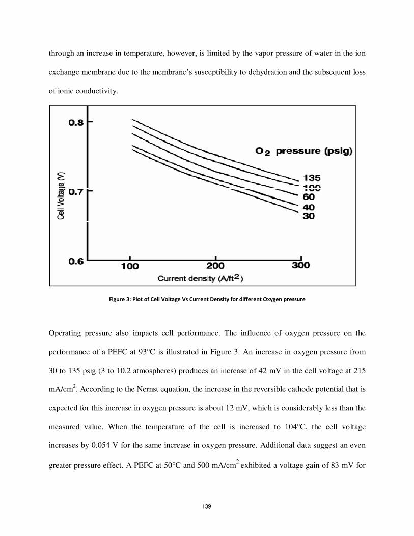
through an increase in temperature, however, is limited by the vapor pressure of water in the ion
exchange membrane due to the membrane’s susceptibility to dehydration and the subsequent loss
of ionic conductivity.
Figure 3: Plot of Cell Voltage Vs Current Density for different Oxygen pressure
Operating pressure also impacts cell performance. The influence of oxygen pressure on the
performance of a PEFC at 93°C is illustrated in Figure 3. An increase in oxygen pressure from
30 to 135 psig (3 to 10.2 atmospheres) produces an increase of 42 mV in the cell voltage at 215
mA/cm2. According to the Nernst equation, the increase in the reversible cathode potential that is
expected for this increase in oxygen pressure is about 12 mV, which is considerably less than the
measured value. When the temperature of the cell is increased to 104°C, the cell voltage
increases by 0.054 V for the same increase in oxygen pressure. Additional data suggest an even
greater pressure effect. A PEFC at 50°C and 500 mA/cm2
exhibited a voltage gain of 83 mV for
139
an increase in pressure from 1 to 5 atmospheres. Another PEFC at 80°C and 431 mA/cm2
showed a voltage gain of 22 mV for a small pressure increase from 2.4 to 3.4 atmospheres. These
results demonstrate that an increase in the pressure of oxygen results in a significant reduction in
polarization at the cathode. Performance improvements due to increased pressure must be
balanced against the energy required to pressurize the reactant gases. The overall system must be
optimized according to output, efficiency, cost, and size.
8.3 PEFC Applications
8.3.1 Transportation Applications
The focus for PEFC applications of PEFC today is on prime power for cars and light trucks.
PEFC is the only type of fuel cell considered for prime motive power in on-road vehicles (as
opposed to APU power, for which SOFC is also being developed). PEFC systems fueled by
hydrogen, methanol, and gasoline have been integrated into light duty vehicles by at least twelve
different carmakers. Early prototypes of fuel cell vehicles (Honda and Toyota) have been
released to controlled customer groups in Japan and the U.S. However, all automakers agree that
the widespread application of PEFC to transportation will not occur until well into the next
decade:
• Volume and weight of fuel cell systems must be further reduced
• Life and reliability of PEFC systems must be improved
140
• PEFC systems must be made more robust in order to be operable under the entire range
of environmental conditions expected of vehicles
• Additional technology development is required to achieve the necessary cost reductions
• A hydrogen infrastructure, and the accompanying safety codes and standards must be
developed.
8.3.2 Stationary Applications
Several developers are also developing PEFC systems for stationary applications. These efforts
are aimed at very small-scale distributed generation (~1 to 10 kW AC). The vast majority of
systems are designed for operation on natural gas or propane. Hundreds of demonstration units
have been sited in programs in the U.S., Europe, and Japan. Typical performance characteristics
are given by Plug Power. Considerable progress has been made in system integration and in
achieving stand-alone operation. System efficiency typically ranges from 25 to 32 percent (based
on LHV). By recovering the waste heat from the cooling water, the overall thermal efficiency
can be raised to about 80 percent, but the water temperature (about 50 to 70 °C) is rather modest
for many CHP applications. System operating life has been extended to about 8,000 hrs for a
single system with a single stack, with degradation of about 5 percent per 1,000 hours.
141
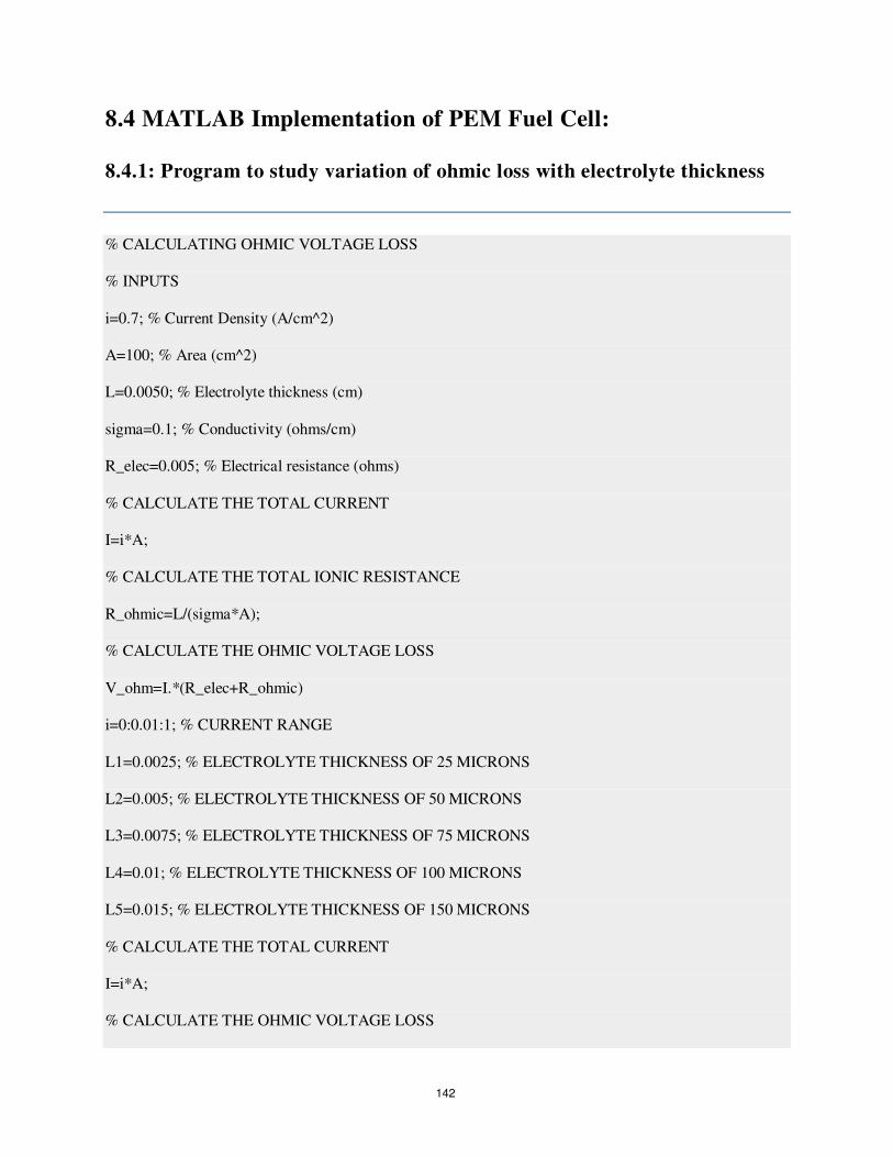
8.4 MATLAB Implementation of PEM Fuel Cell:
8.4.1: Program to study variation of ohmic loss with electrolyte thickness
% CALCULATING OHMIC VOLTAGE LOSS
% INPUTS
i=0.7; % Current Density (A/cm^2)
A=100; % Area (cm^2)
L=0.0050; % Electrolyte thickness (cm)
sigma=0.1; % Conductivity (ohms/cm)
R_elec=0.005; % Electrical resistance (ohms)
% CALCULATE THE TOTAL CURRENT
I=i*A;
% CALCULATE THE TOTAL IONIC RESISTANCE
R_ohmic=L/(sigma*A);
% CALCULATE THE OHMIC VOLTAGE LOSS
V_ohm=I.*(R_elec+R_ohmic)
i=0:0.01:1; % CURRENT RANGE
L1=0.0025; % ELECTROLYTE THICKNESS OF 25 MICRONS
L2=0.005; % ELECTROLYTE THICKNESS OF 50 MICRONS
L3=0.0075; % ELECTROLYTE THICKNESS OF 75 MICRONS
L4=0.01; % ELECTROLYTE THICKNESS OF 100 MICRONS
L5=0.015; % ELECTROLYTE THICKNESS OF 150 MICRONS
% CALCULATE THE TOTAL CURRENT
I=i*A;
% CALCULATE THE OHMIC VOLTAGE LOSS
142
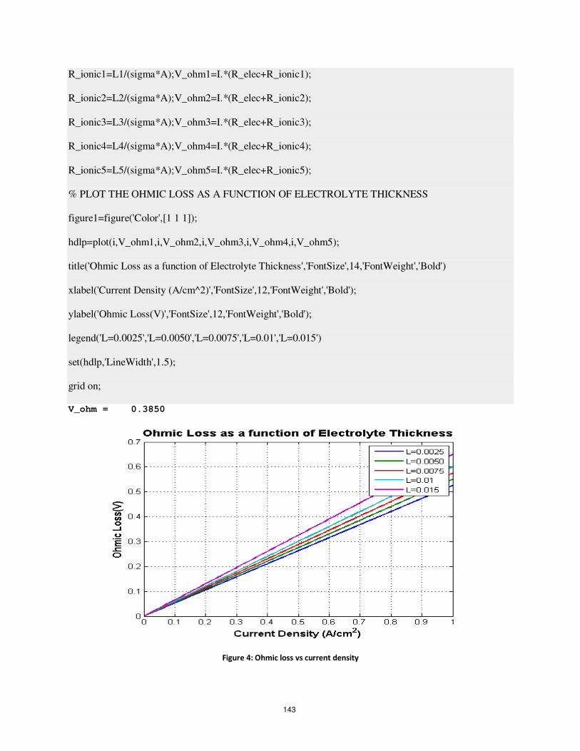
R_ionic1=L1/(sigma*A);V_ohm1=I.*(R_elec+R_ionic1);
R_ionic2=L2/(sigma*A);V_ohm2=I.*(R_elec+R_ionic2);
R_ionic3=L3/(sigma*A);V_ohm3=I.*(R_elec+R_ionic3);
R_ionic4=L4/(sigma*A);V_ohm4=I.*(R_elec+R_ionic4);
R_ionic5=L5/(sigma*A);V_ohm5=I.*(R_elec+R_ionic5);
% PLOT THE OHMIC LOSS AS A FUNCTION OF ELECTROLYTE THICKNESS
figure1=figure('Color',[1 1 1]);
hdlp=plot(i,V_ohm1,i,V_ohm2,i,V_ohm3,i,V_ohm4,i,V_ohm5);
title('Ohmic Loss as a function of Electrolyte Thickness','FontSize',14,'FontWeight','Bold')
xlabel('Current Density (A/cm^2)','FontSize',12,'FontWeight','Bold');
ylabel('Ohmic Loss(V)','FontSize',12,'FontWeight','Bold');
legend('L=0.0025','L=0.0050','L=0.0075','L=0.01','L=0.015')
set(hdlp,'LineWidth',1.5);
grid on;
V_ohm = 0.3850
Figure 4: Ohmic loss vs current density
143

8.4.2: Program to calculate the ohmic losses as a function of fuel cell area.
% CALCULATING THE OHMIC VOLTAGE LOSS WITH DIFFERENT FUEL CELL
% INPUTS
i=0.7; % CURRENT DENSITY (A/cm^2)
R1=0.05; % RESISTANCE (ohms)
A=1:100;
ASR=R1*A;
% CALCULATE THE TOTAL CURRENT
I=i*A;
% CALCULATE THE OHMIC VOLTAGE LOSS
V_ohm=I.*R1;
% PLOT OF THE OHMIC LOSSES AS A FUNCTION OF FUEL CELL AREA
figure1=figure('Color',[1 1 1]);
hdlp=plot(A,V_ohm);
title('Ohmic Loss as a function of Fuel Cell
area','FontSize',14,'FontWeight','Bold')
xlabel('Fuel Cell Area (cm^2)','FontSize',12,'FontWeight','Bold');
ylabel('Ohmic Loss (V)','FontSize',12,'FontWeight','Bold');
set(hdlp,'LineWidth',1.5);
grid on;
144
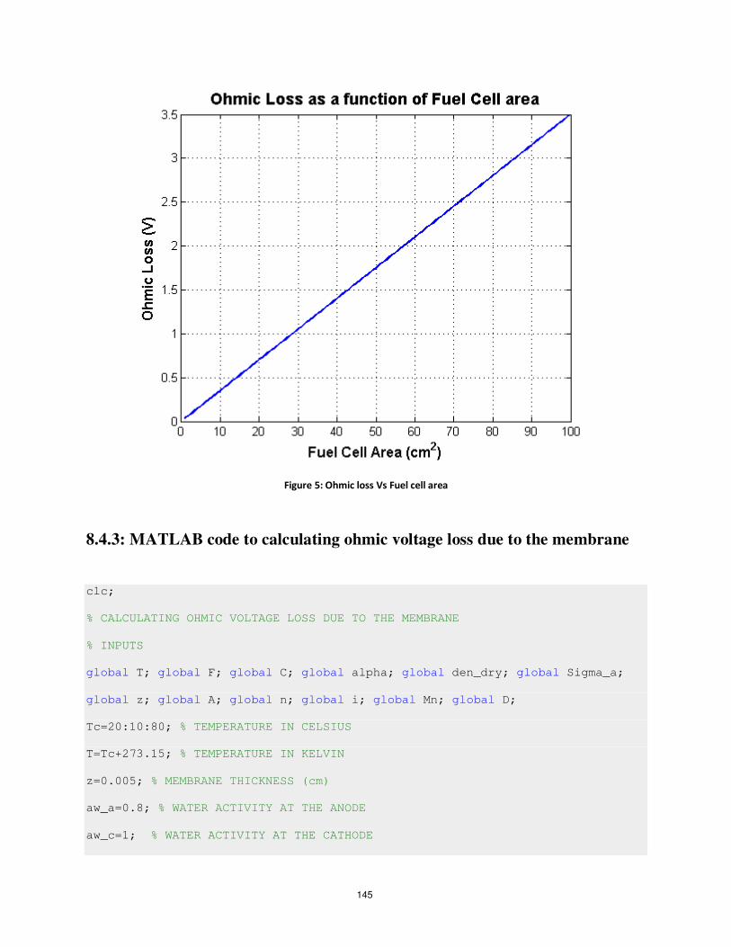
Figure 5: Ohmic loss Vs Fuel cell area
8.4.3: MATLAB code to calculating ohmic voltage loss due to the membrane
clc;
% CALCULATING OHMIC VOLTAGE LOSS DUE TO THE MEMBRANE
% INPUTS
global T; global F; global C; global alpha; global den_dry; global Sigma_a;
global z; global A; global n; global i; global Mn; global D;
Tc=20:10:80; % TEMPERATURE IN CELSIUS
T=Tc+273.15; % TEMPERATURE IN KELVIN
z=0.005; % MEMBRANE THICKNESS (cm)
aw_a=0.8; % WATER ACTIVITY AT THE ANODE
aw_c=1; % WATER ACTIVITY AT THE CATHODE
145

n=2.5; % ELECTRO-OSMOTIC DRAG COEFFICIENT
i=0.8; % CURRENT DENSITY (A/cm^2)
Mn=1; % NAFION EQUIVALENT WEIGHT(kg/mol)
F=96487; % FARADAY'S CONSTANT
den_dry=0.00197; % MEMBRANE DRY DENSITY(kg/cm^3)
C=2.3; % CONSTANT DEPENDENT UPON BOUNDARY CONDITIONS
alpha=1.12; % RATIO OF WATER FLUX TO HYDROGEN FLUX
% CONVERT THE WATER ACTIVITY ON THE NAFION SURFACES TO WATER CONTENTS
lambda_anode=0.043+(17.81*(aw_a))-(39.85*(aw_a^2))+(36*(aw_a^3));
lambda_cathode=0.043+(17.81*(aw_c))-(39.85*(aw_c^2))+(36*(aw_c^3));
% CALCULATE THE WATER DIFFUSIVITY
D=(10.^-6).*exp(2416.*(1./303-1./T)).*(2.563-(0.33.*10)+(0.0264.*10.^2)-
(0.000671.*10.^3));
delta_lambda=((11.*alpha)./n)+C.*exp(((i.*Mn.*n)./(22.*F.*den_dry.*D)).*z);
Sigma_a=exp(1268.*((1./303)-(1./T))).*(0.005139.*delta_lambda-0.00326);%S/m
Sigma_c=exp(1268.*((1./303)-(1./T))).*(0.005139.*delta_lambda-0.00326);%S/m
Re_a=quad('thick',0,0.0050)
V_ohm=i*Re_a
% PLOT
z=0:0.002:0.0125;
delta_lambda=((11.*alpha)./n)+C.*exp(((i.*Mn.*n)./(22.*F.*den_dry.*D)).*z);
Sigma=(1268.*((1./303)-(1./T))).*(0.005139.*delta_lambda-0.00326);% S/m
% PLOT THE MEMBRANE THICKNESS AND WATER CONTENT
figure1=figure('Color',[1 1 1]);
hdlp=plot(z,delta_lambda);
title('Membrane Thickness and Water
content','FontSize',14,'FontWeight','Bold')
xlabel('Membrane Thickness (cm)','Fontsize',12,'FontWeight','Bold');
ylabel('Water Content (H2O/SO3)','Fontsize',12,'FontWeight','Bold');
146
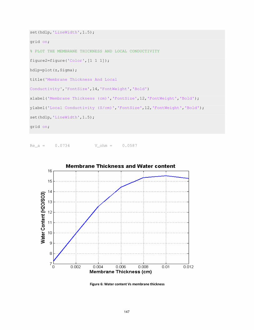
set(hdlp,'LineWidth',1.5);
grid on;
% PLOT THE MEMBRANE THICKNESS AND LOCAL CONDUCTIVITY
figure2=figure('Color',[1 1 1]);
hdlp=plot(z,Sigma);
title('Membrane Thickness And Local
Conductivity','FontSize',14,'FontWeight','Bold')
xlabel('Membrane Thickness (cm)','FontSize',12,'FontWeight','Bold');
ylabel('Local Conductivity (S/cm)','FontSize',12,'FontWeight','Bold');
set(hdlp,'LineWidth',1.5);
grid on;
Re_a = 0.0734 V_ohm = 0.0587
Figure 6: Water content Vs membrane thickness
147
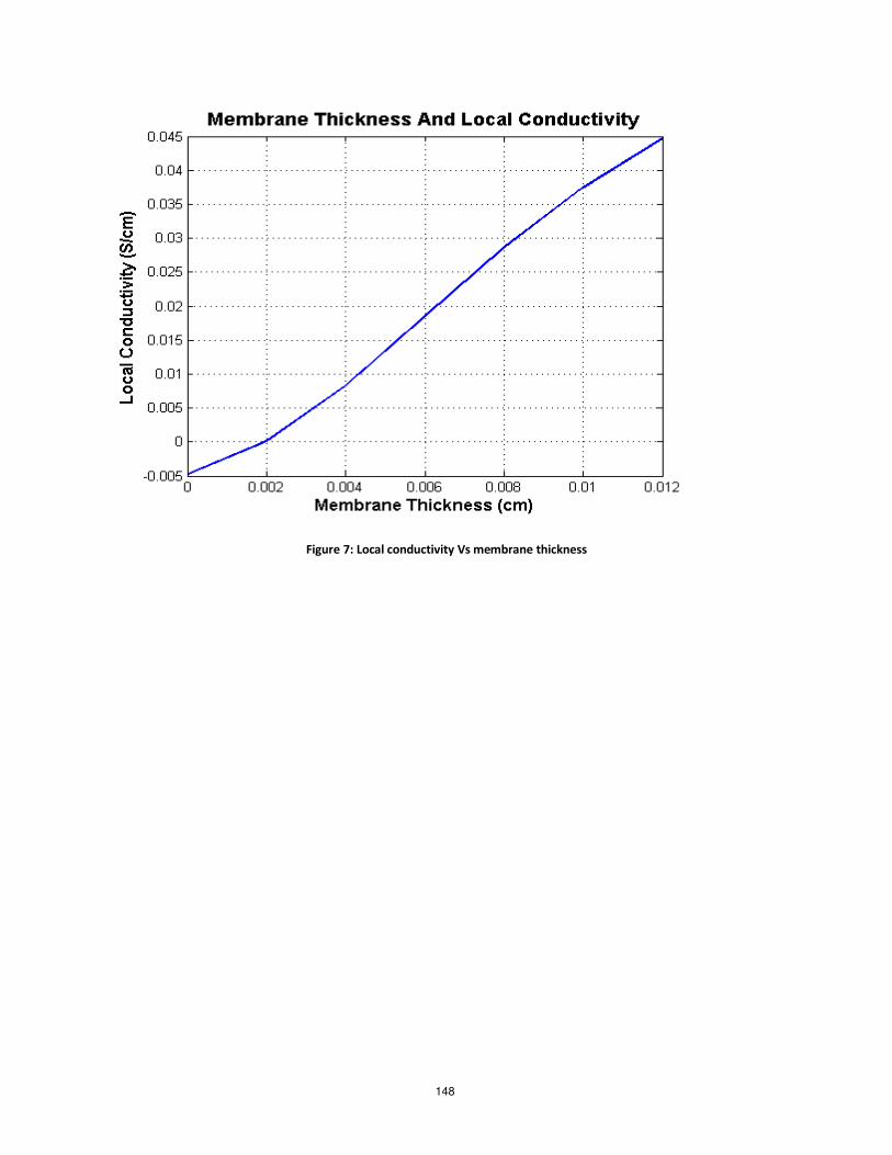
Figure 7: Local conductivity Vs membrane thickness
148
8.5 References
1. S. Gottesfeld, “The Polymer Electrolyte Fuel Cell: Materials Issues in a Hydrogen Fueled
Power Source,” LANL, undated.
2. W.T. Grubb, Proceedings of the 11th Annual Battery Research and Development
Conference, PSC Publications Committee, Red Bank, NJ, p. 5, 1957; U.S. Patent No.
2,913,511, 1959.
3. Communication with Plug Power, August 2002.
4. W.D. Ernst, Patent No. 5,912,088, Plug Power Inc., June 15, 1999.
5. G.S. Eisman, et al., Patent No. 6,280,865, Plug Power Inc., August 28, 2001.
6. W.G.F. Grot, G.E. Munn, P.N. Walmsley, paper presented at the 141st National Meeting of
the Electrochemical Society, Inc., Abstract No. 154, Houston, TX, May 7-11, 1972.
7. T. Ralph, "Proton Exchange Membrane Fuel Cells: Progress in Cost Reduction of the Key
Components," Platinum Metals Review, 41, pp. 102-113, 1997.
8. B.R. Ezzell, B. Carl, and W. Mod, Ion Exchange Membranes for the Chlor Alkali Industry,
AIChE Symp. Series, Houston, TX, March 1985, Pg. 49
9. K. Prater, "The Renaissance of the Solid Polymer Fuel Cell," Ballard Power Systems, Inc.,
Journal of Power Sources, p. 29, 1990.
10. D.J. Wheeler, J.S. Yi, R. Fredley, D. Yang, T. Patterson Jr., L. VanDine, “Advacements in
Fuel cell Stack Technology at International Fuel Cells,” International Fuel Cells (now UTC
Fuel Cells), Journal of New Materials for Electrochemical Systems, 4, 2001.
11. Peter M. Schutz, A Preliminary Investigation of Radiation Catalysts in Fuel Cells, Master of
Science Thesis, Virginia Polytechnic University, Blacksburg, Va., August, 1979 Pg. 59.
149
12. 3M Product Bulletin, date unknown.
13. D. S. Watkins, et al., Abstracts 37th International Power Sources Symposium (The
Electrochemical Society) p. 782, 1988.
14. Lousenberg, D., et al. Diferentiated Membranes and Dispersions for Commercial PEM Fuel
Cell and Electrolysis Systems. in 2003 Fuel Cell Seminar. 2003. Miami Beach, FL, USA:
Department of Energy.
15. Teather, E. and J. Staser. MEA Improvements for Sub-humidified Fuel Cell Operation. In
2003 Fuel Cell Seminar. 2003. Miami Beach, FL, USA: Department of Energy.
16. Cleghorn, S., et al. New MEAs for Low Cost System Design. in 2003 Fuel Cell Seminar.
2003. Miami Beach, FL, USA: Department of Energy.
150

CONCLUSION AND SCOPE FOR FUTURE WORK
India has enormous potential for development in solar power due to large number of sunny days per year
and a large mainland area. Solar thermal energy is an easy and economical source of electrical power. For
large power requirement, solar central receiver is suitable. India ranks 4th in the world in terms of existing
capacity and 3rd
in terms of new wind power added. Newton- Raphson method if applied will give
convergence in less iteration compared to G-S method.
As I have made a feasibility study of setting up a Photovoltaic plant at Rourkela, A local contractor can
be hired to build a pole kit with PV modules mounted above the lamp and the battery enclosure
mounted to the pole near ground level. The modules are prewired and assembled in an
Aluminum frame that is attached to the pole at the proper tilt angle. The array conductors can be
run down the inside of the metal pole to the control box mounted to the pole behind the battery
enclosure. The battery box can be shaded with a metal overhang to maintain ambient
temperature. To protect the poles from lightning, lightning rods can be attached.
Solar photovoltaic power can be used at remote villages to provide light during night-time. This will
promote literacy among village children and encourage men &women to take up handicraft work as an
option to earn extra money. A survey in this regard can be made. Also, solar electricity can be used to
drive motor to pump water during day. This will reduce peak load on grid and ensure lesser power cuts.
151
References
1. Georg Hille, Werner Roth, and Heribert Schmidt, ‘‘Photovoltaic systems,’’ Fraunhofer
Institute for Solar Energy Systems, Freiburg, Germany, 1995.
2. OKA Heinrich Wilk, ‘‘Utility connected photovoltaic systems,’’ contribution to design
handbook, Expert meeting Montreux, October 19–21, 1992, International Energy Agency (IEA):
Solar Heating and Cooling Program.
3. Stuart R. Wenham, Martin A. Green, and Muriel E. Watt, ‘‘ Applied photovoltaics,’’ Centre
for photovoltaic devices and systems, UNSW.
4. N. Ashari, W. W. L. Keerthipala, and C. V. Nayar, ‘‘A single phase parallel connected
Uninterruptible power supply/Demand side management system,’’ PE-275-EC (08-99), IEEE
Transactions on Energy Conversion, August 1999.
5. C. V. Nayar, and M. Ashari, ‘‘Phase power balancing of a diesel generator using a bi-
directional PWM inverter,’’ IEEE Power Engineering Review 19 (1999).
6. C. V. Nayar, J. Perahia, S. J. Philips, S. Sadler, and U. Duetchler, ‘‘Optimized power
electronic device for a solar powered centrifugal pump,’’ Journal of the Solar Energy Society of
India, SESI Journal 3(2), 87–98 (1993).
7. Ziyad M. Salameh, and Fouad Dagher, ‘‘The effect of electrical array reconfiguration on the
performance of a PV-powered volumetric water pump,’’ IEEE Transactions on Energy
Conversion 5 653–658 (1990).
152
8. C. V. Nayar, S. J. Phillips, and W. L. James, T. L. Pryor, D. Remmer, ‘‘Novel
wind/diesel/battery hybrid system,’’ Solar Energy 51, 65–78 (1993).
9. W. Bower, ‘‘Merging photovoltaic hardware development with hybrid applications in the
U.S.A.’’ Proceedings Solar ’93 ANZSES, Fremantle, Western Australia (1993).
10. Ned Mohan, M. Undeland, and W. P. Robbins, ‘‘Power Electronics,’’ 2nd ed. John Wiley
and Sons, Inc. (1995).
11. M. Calais, V. G. Agelidis, M. Meinhardt, ‘‘Multilevel Converters for single phase grid
connected photovoltaic systems—an overview,’’ Solar Energy 66, 325–535 (1999).
12. K. Hirachi, K. Matsumoto, M. Yamamoto, and M. Nakaoka, ‘‘Improved control
implementation of single phase current fed PWM inverter for photovoltaic power generation,’’
Seventh International Conference on Power Electronics and Variable Speed drives (PEVD’98).
13. U. Boegli and R. Ulmi, ‘‘Realisation of a new inverter circuit for direct photovoltaic energy
feedback into the public grid,’’ IEEE Transactions on Industry Application, March/April (1986).
14. B. Lindgren, ‘‘Topology for decentralised solar energy inverters with a low voltage A-Bus:
EPE99 (European Power Electronics Conference) (1999).
15. Khalid Masoud and Gerard Ledwich, ‘‘Aspects of grid interfacing: current and voltage
controllers,’’ Proceedings of AUPEC 99, pp 258–263.
16. J. F. Lindsay and M. H. Rashid, ‘‘Electro-mechanics and Electrical Machinery,’’ Prentice
Hall Inc., 1986.
153
17. Lawrence J. Borle and Michael S. Dymond, Chemmangot V. Nayar, ‘‘Development and
testing of a 20 kW grid interactive photovoltaic power conditioning system in Western
Australia,’’ IEEE Transactions on Industry Applications 33, 1–7 (1999).
18. Lawrence J. Borle and C. V. Nayar, ‘‘Zero average current error controlled power flow for
ac–DC power converters,’’ IEEE Transactions on Power Electronics 10, 725–732 (1995).
19. Hari Sharma, ‘‘Grid integration of photovoltaics,’’ Ph.D. thesis, The University of
Newcastle, Australia (1998).
20. D. Langridge, W. Lawrance, and B. Wichert, ‘‘Development of a photo-voltaic pumping
system using a brushless D.C. motor and helical rotor pump,’’ Solar Energy 56, 151–160 (1996).
21. Donald Paul Hodel, ‘‘Photovoltaics—Electricity from sunlight,’’ U.S. Department of Energy
report, DOE/NBMCE-1075.
22. Rao S., Parulekar B.B.: Energy Technology
23. Rai G.D.: Non Conventional Energy Sources
24. Carlson, D. E. 1995. “Recent Advances in Photovoltaics,” 1995 Proceedings of the
Intersociety Engineering Conference on Energy Conversion 1995, p. 621-626.
25. Akshay Urja: A newsletter of the Ministry of New and Renewable Energy, Government of
India.
26. Stand-alone photovoltaic systems: A handbook of recommended design practices, Issued by
Sandia National Laboratories operated for the United States Department of Energy by Sandia
Corporation
154

27. www.google.com
28. www.en-wikipedia.org
29. Booklets from Ministry of Non-Conventional Energy Sources
155

Appendix
156
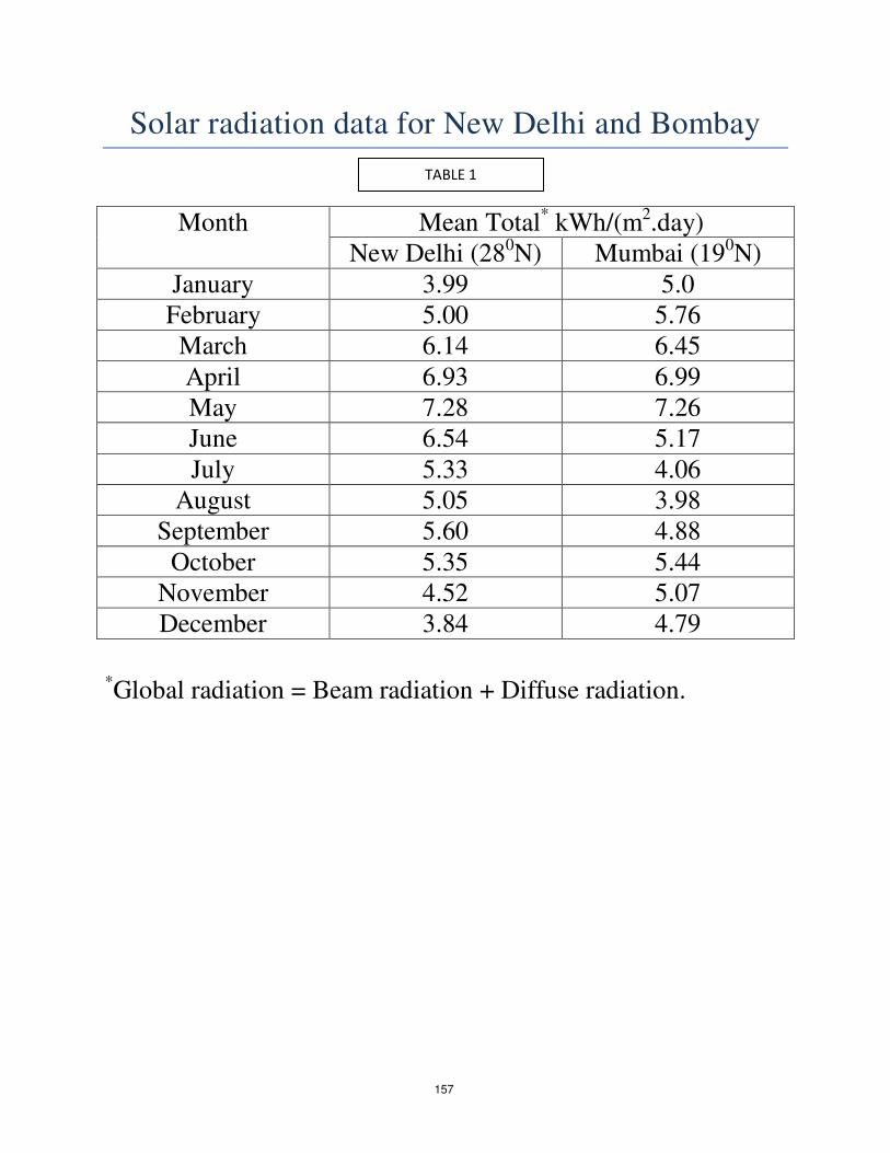
Solar radiation data for New Delhi and Bombay
Month Mean Total* kWh/(m2.day)
New Delhi (280N) Mumbai (190N)
January 3.99 5.0
February 5.00 5.76
March 6.14 6.45
April 6.93 6.99
May 7.28 7.26
June 6.54 5.17
July 5.33 4.06
August 5.05 3.98
September 5.60 4.88
October 5.35 5.44
November 4.52 5.07
December 3.84 4.79
*Global radiation = Beam radiation + Diffuse radiation.
TABLE 1
157
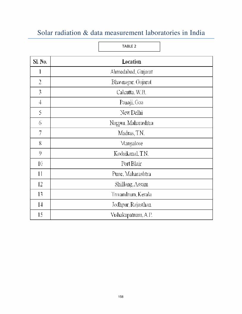
Solar radiation & data measurement laboratories in India
TABLE 2
158
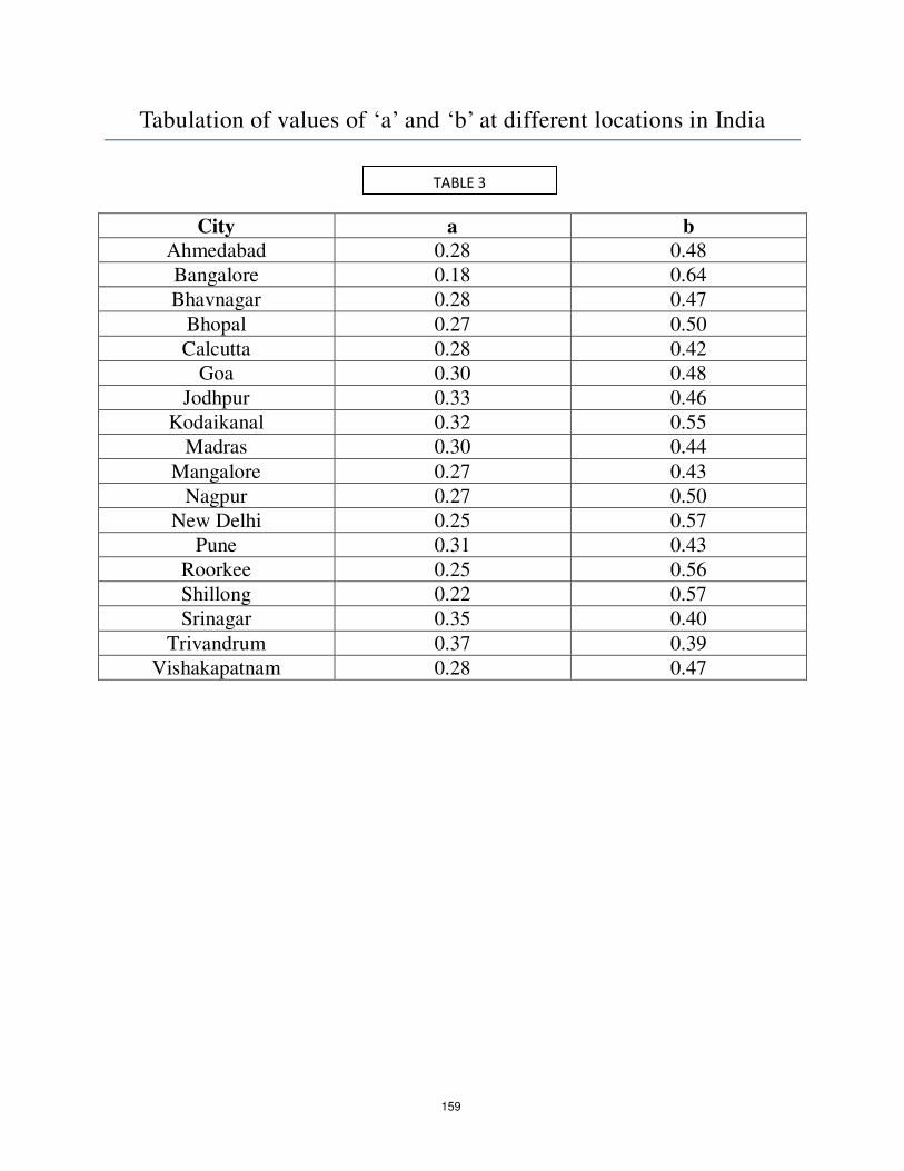
Tabulation of values of ‘a’ and ‘b’ at different locations in India
City a b
Ahmedabad 0.28 0.48
Bangalore 0.18 0.64
Bhavnagar 0.28 0.47
Bhopal 0.27 0.50
Calcutta 0.28 0.42
Goa 0.30 0.48
Jodhpur 0.33 0.46
Kodaikanal 0.32 0.55
Madras 0.30 0.44
Mangalore 0.27 0.43
Nagpur 0.27 0.50
New Delhi 0.25 0.57
Pune 0.31 0.43
Roorkee 0.25 0.56
Shillong 0.22 0.57
Srinagar 0.35 0.40
Trivandrum 0.37 0.39
Vishakapatnam 0.28 0.47
TABLE 3
159
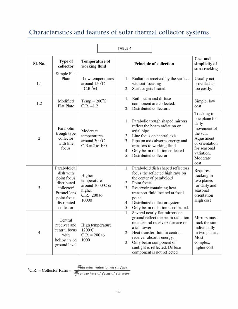
Characteristics and features of solar thermal collector systems
Sl. No. Type of
collector
Temperature of
working fluid Principle of collection
Cost and
simplicity of
sun-tracking
1.1
Simple Flat Plate
-Low temperatures
around 1500C
- C.R.#=1
1. Radiation received by the surface
without focusing
2. Surface gets heated.
Usually not
provided as
too costly.
1.2 Modified Flat Plate
Temp = 2000C
C.R. =1.2
1. Both beam and diffuse
component are collected.
2. Distributed collectors.
Simple, low cost
2
Parabolic trough type
collector
with line focus
Moderate
temperatures around 300
0C
C.R.= 2 to 100
1. Parabolic trough shaped mirrors reflect the beam radiation on
axial pipe.
2. Line focus on central axis. 3. Pipe on axis absorbs energy and
transfers to working fluid
4. Only beam radiation collected 5. Distributed collector.
Tracking in
one plane for
daily
movement of the sun,
Adjustment
of orientation for seasonal
variation,
Moderate
cost
3
Paraboloidal
dish with
point focus distributed
collector/
Fresnel lens
point focus distributed
collector
Higher
temperature
around 10000C or
higher
C.R.=200 to
10000
1. Paraboloid dish shaped reflectors
focus the reflected high rays on
the center of paraboloid 2. Point focus
3. Reservoir containing heat
transport fluid located at focal
point 4. Distributed collector system
5. Only beam radiation is collected.
Requires tracking in
two planes
for daily and seasonal
orientation
High cost
4
Central receiver and
central focus
with
heliostats on ground level
High temperature
12000C
C.R. = 200 to
1000
1. Several nearly flat mirrors on ground reflect the beam radiation
on a central receiver/ furnace on
a tall tower.
2. Heat transfer fluid in central receiver absorbs energy.
3. Only beam component of
sunlight is reflected. Diffuse component is not reflected.
Mirrors must
track the sun
individually
in two planes, Most
complex,
higher cost
#C.R. = Collector Ratio =
TABLE 4
160
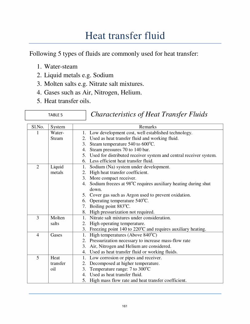
Heat transfer fluid
Following 5 types of fluids are commonly used for heat transfer:
1. Water-steam
2. Liquid metals e.g. Sodium
3. Molten salts e.g. Nitrate salt mixtures.
4. Gases such as Air, Nitrogen, Helium.
5. Heat transfer oils.
Characteristics of Heat Transfer Fluids
Sl.No. System Remarks
1 Water-
Steam
1. Low development cost, well established technology.
2. Used as heat transfer fluid and working fluid.
3. Steam temperature 540 to 600oC.
4. Steam pressures 70 to 140 bar.
5. Used for distributed receiver system and central receiver system.
6. Less efficient heat transfer fluid.
2 Liquid
metals
1. Sodium (Na) system under development.
2. High heat transfer coefficient.
3. More compact receiver.
4. Sodium freezes at 98oC requires auxiliary heating during shut
down.
5. Cover gas such as Argon used to prevent oxidation.
6. Operating temperature 540oC.
7. Boiling point 883oC.
8. High pressurization not required.
3 Molten
salts
1. Nitrate salt mixtures under consideration.
2. High operating temperature.
3. Freezing point 140 to 220oC and requires auxiliary heating.
4 Gases 1. High temperatures (Above 840oC)
2. Pressurization necessary to increase mass-flow rate
3. Air, Nitrogen and Helium are considered.
4. Used as heat transfer fluid or working fluids.
5 Heat
transfer
oil
1. Low corrosion or pipes and receiver.
2. Decomposed at higher temperature.
3. Temperature range: 7 to 300oC
4. Used as heat transfer fluid.
5. High mass flow rate and heat transfer coefficient.
TABLE 5
161
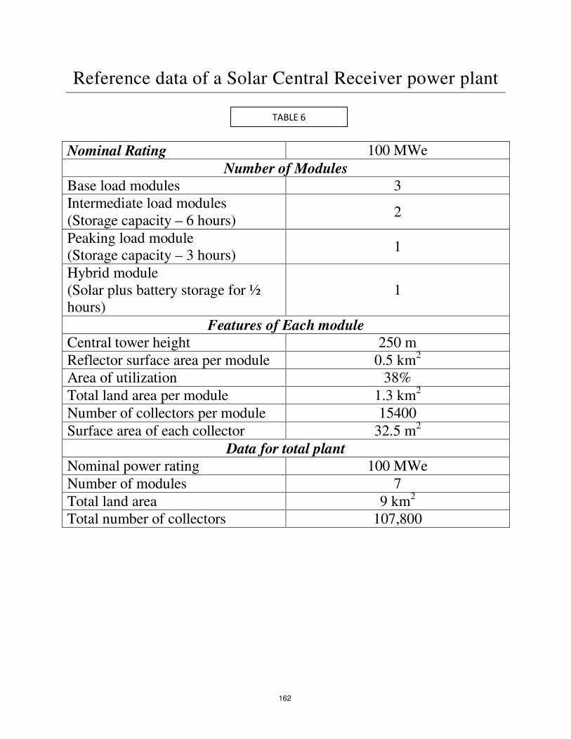
Reference data of a Solar Central Receiver power plant
Nominal Rating 100 MWe
Number of Modules
Base load modules 3
Intermediate load modules
(Storage capacity – 6 hours) 2
Peaking load module
(Storage capacity – 3 hours) 1
Hybrid module
(Solar plus battery storage for ½
hours)
1
Features of Each module
Central tower height 250 m
Reflector surface area per module 0.5 km2
Area of utilization 38%
Total land area per module 1.3 km2
Number of collectors per module 15400
Surface area of each collector 32.5 m2
Data for total plant
Nominal power rating 100 MWe
Number of modules 7
Total land area 9 km2
Total number of collectors 107,800
TABLE 6
162
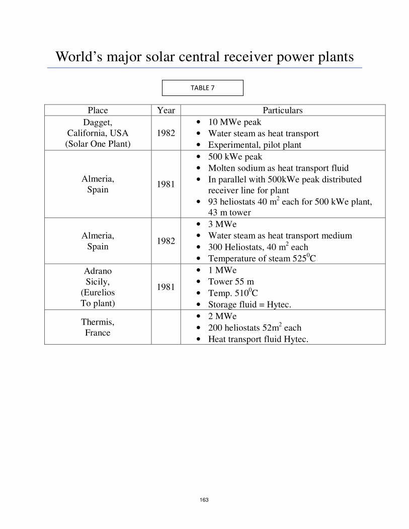
World’s major solar central receiver power plants
Place Year Particulars
Dagget,
California, USA
(Solar One Plant)
1982
• 10 MWe peak
• Water steam as heat transport
• Experimental, pilot plant
Almeria,
Spain 1981
• 500 kWe peak
• Molten sodium as heat transport fluid
• In parallel with 500kWe peak distributed
receiver line for plant
• 93 heliostats 40 m2 each for 500 kWe plant,
43 m tower
Almeria,
Spain 1982
• 3 MWe
• Water steam as heat transport medium
• 300 Heliostats, 40 m2 each
• Temperature of steam 5250C
Adrano
Sicily,
(Eurelios
To plant)
1981
• 1 MWe
• Tower 55 m
• Temp. 5100C
• Storage fluid = Hytec.
Thermis,
France
• 2 MWe
• 200 heliostats 52m2 each
• Heat transport fluid Hytec.
TABLE 7
163
Intermediate Compounds
Any of types of Silicon (Homo-crystalline, poly-crystalline,
Amorphous) are treated with any of the following intermediate
compounds to form N-P junctions:
1. Cadmium-Sulphide
2. Gallium-Arsenide
3. Zinc-Sulphide
4. Gallium-Antimonide
5. Cadmium-Territide
6. Indium-Phosphate
7. Cadmium-Selenide
164

Efficiency of a solar cell
Efficiency = ()
()
A PV cell must be operated at knee point with maximum possible incident
light for obtaining maximum power and therefore high efficiency.
Maximum efficiency achieved in laboratories is 15-20 %. Maximum
theoretical possible efficiency is 25%.
Cell Efficiency 1980s With amorphous silicon 5%
With polycrystalline silicon 7%
With single crystalline silicon 12%
#Efficiency of solar PV module is lesser than cell efficiency due to lesser area coverage factor ( Solar cell area/ module area ).
TABLE 8
165
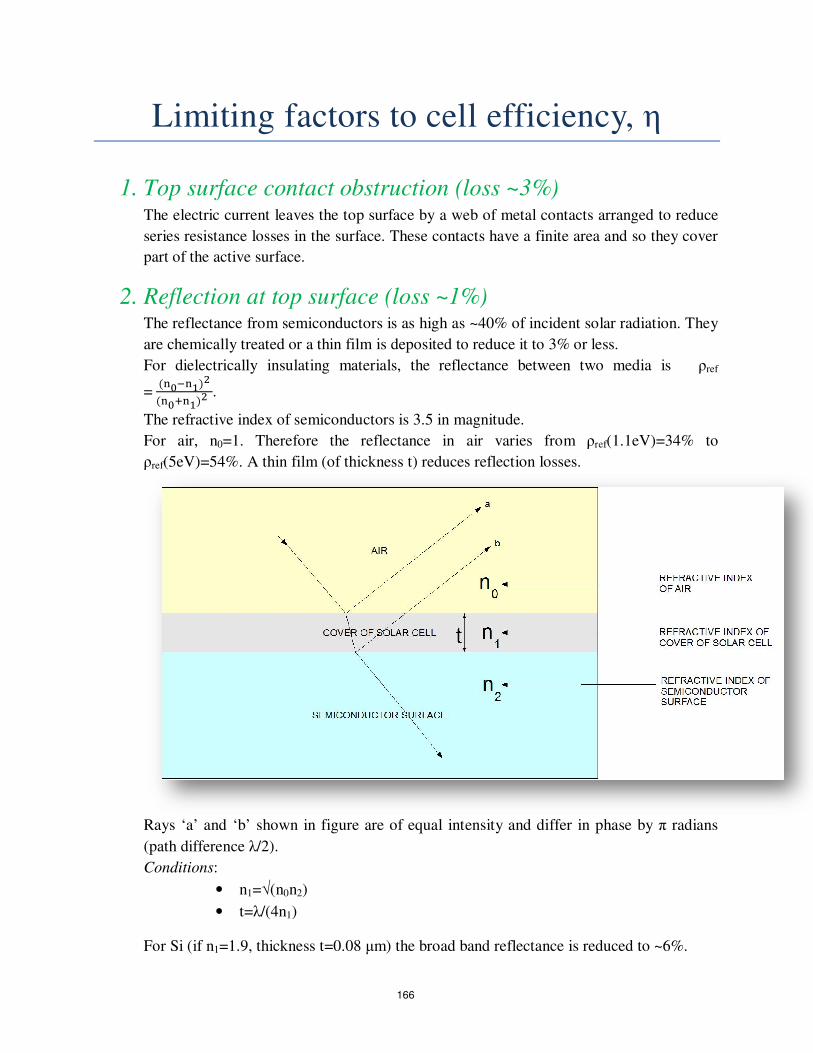
Limiting factors to cell efficiency, η
1. Top surface contact obstruction (loss ~3%) The electric current leaves the top surface by a web of metal contacts arranged to reduce
series resistance losses in the surface. These contacts have a finite area and so they cover
part of the active surface.
2. Reflection at top surface (loss ~1%) The reflectance from semiconductors is as high as ~40% of incident solar radiation. They
are chemically treated or a thin film is deposited to reduce it to 3% or less.
For dielectrically insulating materials, the reflectance between two media is ρref
= ()
( ) .
The refractive index of semiconductors is 3.5 in magnitude.
For air, n0=1. Therefore the reflectance in air varies from ρref(1.1eV)=34% to
ρref(5eV)=54%. A thin film (of thickness t) reduces reflection losses.
Rays ‘a’ and ‘b’ shown in figure are of equal intensity and differ in phase by π radians
(path difference λ/2).
Conditions:
• n1=√(n0n2)
• t=λ/(4n1)
For Si (if n1=1.9, thickness t=0.08 µm) the broad band reflectance is reduced to ~6%.
166
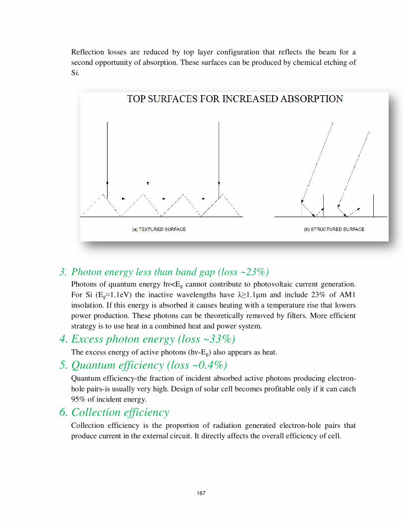
Reflection losses are reduced by top layer configuration that reflects the beam for a
second opportunity of absorption. These surfaces can be produced by chemical etching of
Si.
3. Photon energy less than band gap (loss ~23%) Photons of quantum energy hν<Eg cannot contribute to photovoltaic current generation.
For Si (Eg≈1.1eV) the inactive wavelengths have λ≥1.1µm and include 23% of AM1
insolation. If this energy is absorbed it causes heating with a temperature rise that lowers
power production. These photons can be theoretically removed by filters. More efficient
strategy is to use heat in a combined heat and power system.
4. Excess photon energy (loss ~33%) The excess energy of active photons (hν-Eg) also appears as heat.
5. Quantum efficiency (loss ~0.4%) Quantum efficiency-the fraction of incident absorbed active photons producing electron-
hole pairs-is usually very high. Design of solar cell becomes profitable only if it can catch
95% of incident energy.
6. Collection efficiency Collection efficiency is the proportion of radiation generated electron-hole pairs that
produce current in the external circuit. It directly affects the overall efficiency of cell.
167
7. Voltage factor FV (loss ~4%)
Each absorbed photon produces electron-hole pairs with a constant potential difference but
only a portion of it is available for EMF in the external circuit.
The voltage factor is FV=!"
#$.
In Si, FV ranges from ~0.6 (0.01Ωm material) to ~0.5 (0.1Ω m material).
This result in production of VB≈ 0.66 to 0.55 V.
When producing current under load, heat is produced due to movement of carriers.
8. Curve factor FC (loss ~4%)
I-V characteristic of a solar cell depends on p-n junction characteristics and therefore, peak
power Pm is less than the product of ISCVOC as
I=I0.exp[ &V
(A)T)
- 1] - IL
Curve factor is given as FC =+,-. IscVoc⁄ and is maximum 0.88 for Si.
9. Additional curve factor ‘A’ (loss ~5%)
The factor ‘A’ results in cell due to increased recombination. This tends to change VOC and
ISC as a result maximum power output is when A=1.
10. Series resistance (loss ~0.3%)
The solar cell current passes through a circuit having non-uniform resistance. The exposed
surface is made maximum to absorb large solar insolation but the contacts are made thin for
low contact loss. The power loss is equivalent of a series resistor present in a circuit wasting
energy. Surface layouts are changed to reduce the series resistance to 0.1Ω in a cell of
resistance 20Ω.
11. Shunt resistance (loss ~0.1%)
Shunt resistance appear in circuit due to imperfections on structure of edge of cell.
However this results in negligible loss. For single crystal Si cell, shunt resistance is
considered infinite. But this is not true in polycrystalline cells.
168