-e

NON BALANCED EXPERIMENTAL DESIGNS FORESTIMATING VARIANCE COMPONENTS

by

R. L. Anderson

Presented at Seminar on Sampling of Bulk MaterialsTokyo, Japan, November 15-18, 1965, sponsored by theNational Science Foundation and the Japan Societyfor the Promotion of Science.

Institute of Statisticsl{tmeograph Series 452

NON BALANCED EXPERD1ENTAL DESIGNS FOR

ESTIMATING VARIANCE COMPONEln'S*R. L. Anderson

North Carolina state University at RaleighRaleigh, North carolina

1. Introduction

This paper is a summary of recent reeearch at North Carolina State University

on the development of experimental designs to estimate variance components. Much of

the research has been conducted by doctoral candidates in Experimental Statistics

under my direction. The two most recent projects are not completed, but developments

to date are summarized here. In our experience, a knowledge of the magnitude of the

variance components would be useful in the following situations:

(1) Population changes often can be described in terms of variance components, e.g.,

in quantitative genetics. Hence a knowledge of the actual magnitude of these

components is reqUired in assessing various control programs.

The proper allocation of resources to reduce product variability depends on a

knowledge of the relative magnitude of the variance components.

t~) A knowledge of the relative magnitude of the variance components is also needed

to determine the best allocation of funds in sampling to estimate population

means and totals and in planning experiments to compare treatments.

Unfortunately I have had very little experience with the problems faced in the

sampling of bulk materials. It is hoped that my appearance on this symposium will

have two benefits:

(a) Enable me to become familiar with your problems so that some of our

research can be oriented in the direction of helping to solve them.

* Presented at Seminar on Sampling of :Bulk Materials, Tokyo, Japan, November 15-18, 1965;sponsored by the National Science Foupdation and the Japan Society for the Promotionof Science.'e, ",>\1,#$

2

(b) Furnish you with a brief description of current devel~ents in designing

experiments to estimate variance components in the hope that you will be

able to adapt some of the results to bulk swmpling situations.

In this paper, it will be assumed that all sources of variation are essentially

random. Two experimental and operational procedures are considered: the nested or

hierarchical type and the classification type. A balanced nested design and a two­

way classification operation with nested-type sub-sampling are illustrated in Table ~.

I have been using as a typical example of a nested-type operation the following:

A pilot study was considered to assess the various sources of variability in the

production and assay for streptomycin before conducting an experiment on the efficacy

of various molds. There were five stages in this process: an initial incubation in

a test tube; a primary inoculation period in a petrie dish; a secondary inoculation

period in another petrie dish; a fermentation period in a bath; and the final assay

of the amount of streptomycin produced. This is a five-stage nested operation.

Another example is a study by Newton, et ale (1951) of the variability of rubber,

considering the following sources of variation: producer's estates, days at a given

estate, bales on a given day, sheets from a given bale, and samples from each sheet.

Technicians then took measurements on the samples.

As an example of a classification-type operation, consider the follOWing: Samples

from each of s =10 sources of a material are to be analyzed by each of f =5 labora­

tories. Let us assume that n ;:; 2 samples are sent to each laboratory from each

source. This is a two-way classification operation. The purpose of the investigation

is to est1ma~e the lab-to-lab variation, the source-to-source variation, a possible

lab x source interaction (the failure of source differences to be the same from lab

to lab~ and the swmple-to-sample variation. It is also possible to determine if the

sample-to-sample variation is constant from lab to lab or source to source.

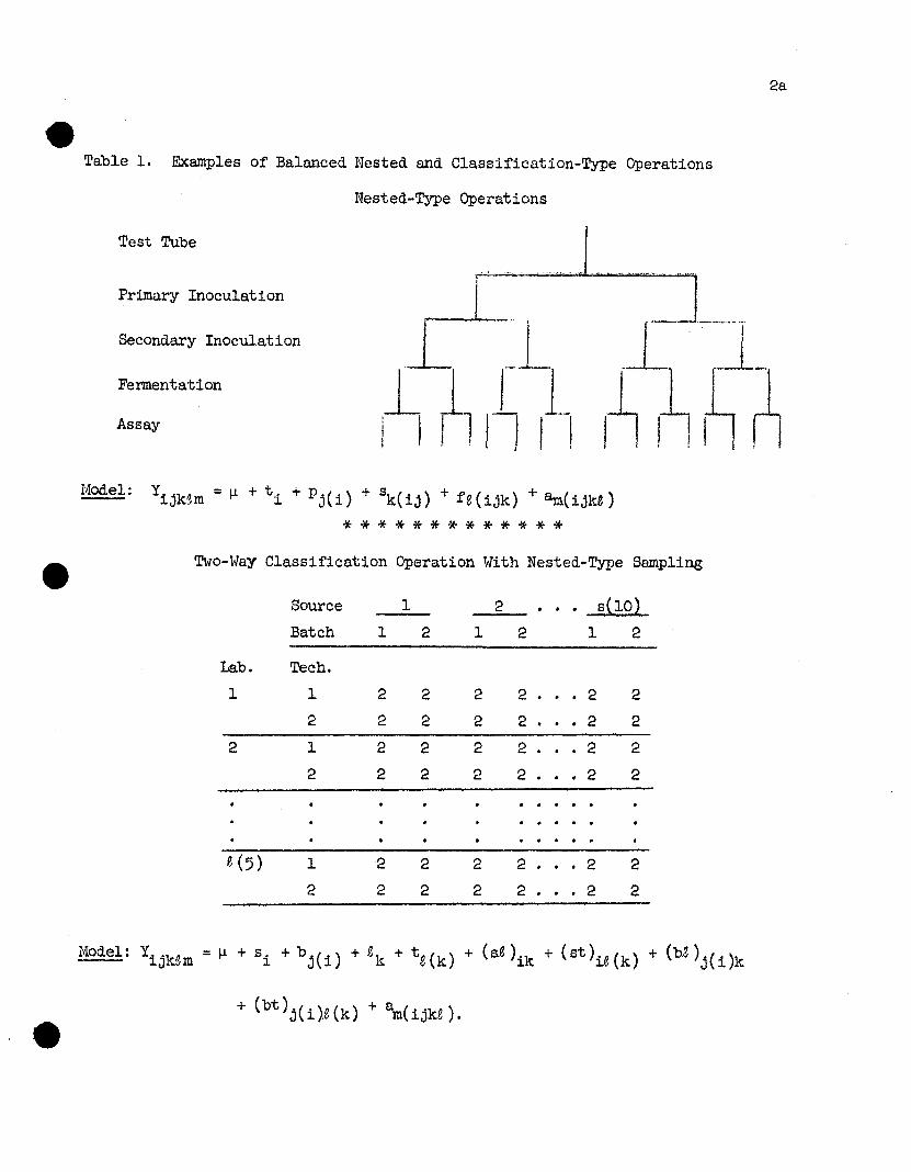
Table 1. Examples of Balanced Nested and Classification-Type Operations

Nested-Type Operations

2a

Test Tube

Primary Inoculation

Secondary Inoculation

Fermentation

Assay

~' ...,

Nodel: Yijk~m = I..l + t i + Pj(i) + sk(1j) + fe(ijk) + B.m(ijkt)

*************Two-Way Classification Operation With Nested-Type Sampling

5(10)

1 2

Source

Batch

Lab. Tech.

1 1

2

2 1

2

1

2

1

2

2

2

2

2

2

1

2

2

2

2

2

2

2

1

2

2

2

2

2

2

2 . . .2

2 . 2

2 ••• 2

2 • • • 2

2 • • • 2

. . . . .2 • • • 2

2 . 2

2

2

2

2

2

2

for example, Pj(i) is the

.3

Additional complications can be added to the last example1 which involve com­

binations of nested and classification-type operations. Suppose each laboratory

selects 2 technicians for the study and from each source 2 batches are selected. In

this case1 4 samples are sent to each laboratory from each batch, 2 for each tech-

nician.

Many classification-type operations will involve more than two classes. Some

discussion of the general multi-way classification operation will be included in

this paper.

The stochastic models for the observations obtained by use of these operations

are given at the bottom of each example in Table 1. In all cases ~ is the general

mean and the other parts of the models are assumed to be independently identically

distributed random variables. We will assume these random variables are normally

distributed; however1 this requirement is Bot always essential. The parameters of

e interest are the variances of the random variables. For the nested-type operation,

these are

For the two-way classification operation, they are

22 22 22 2 2 20s'Ob(s),og,Ot(K),C1sf,Ost(£),ob(s)K,ab(s)t(J.) ~ C1a •

The notation j(i) means the jth sample in the i th class;

th thj primary inoculation sample from the i test tube.

If only one batch is used per source and one technician per lab, one will not be

able to separate batch and source variation or technician and lab variation. The

model might be written in this manner

Yikm = ~ + S1 + ~ + (SL)ik + am(ik) I

222 2 2 2where 1n this case Os is the sum of as and C\ above, 0L is the sum of OK and at and

2C1SL the sum of the interaction components.

4

Suppose we have i incubation test tUbes and select two samples from each for the

primary inoculation, two from each primary for the secondary, two from each secondary

for the fermentation bath and assay two samples from each fermentation bath, giving

a total of l6t assays. The analyses of variance and the accompanying average values

of the mean squares are given in Table 2 for data obtained from balanced nested,

simple two-way classification and combined nested-classification designs.

An examination of these analyses of variance reveals that a balanced design will

concentrate most of the information on the estimation of (J2 and only a small amounta2

of information on the estimation of some of the other variance components, e.g., (Jt

and (J~ for the nested design and (J;,(J~(s),(Jt' and (J~(f) for the classification

designs. In order to more nearly balance the information on the various estimators)

some form of non-balanced design is necessary. The decision as to how to construct

a non-balanced design is complicated by a number of questions, e.g.,

1) What is the best estimation procedure for a non-balanced design?

2) What criteria of efficiency should be used When a number of variance

components, plus the general mean, must be estimated? In this con-

text, it should be noted that in many cases it is ratios of variance

components which are of most importance to the investigator.

3) How much will comparisons of different designs be affected by

total sample size and by the values of the parameters to be estimated?

4) How will these results depend on different sampling cost functions?

5) If the optimal results depend on the values of the parameters being

estimated, would a sequential plan be useful? Or should one con-

sider some form of Bayesian estimation?

One might recommend that maximum likelihood (ML) procedures should be used;

however, these produce equations which are non-linear in the estimators and for

4a

~ Table 2. Analyses of Variance for Balanced Nested and Classification-Type Data

5-stage nested operation with (t,2,2,2,2) successive samples

Degrees ofFreedom

Coefficients of variancecomponents in averagevalue of mean square.2 2 2 2 2

a a~ a a 0ta Jo s P- -.- --t - 1 1 2 4 8 16

t 1 2 4 82t 1 2 44t 1 28t 1

**************

Source of variation

IncubationPrimary InoculationSecondary InoculationFermentationAssay

,Two-way classification operation

Source ofVariation

SourcesLabsS x LAnalyses*

Degrees ofFreedom

s-1(9)e-1(4)

(8-1)( ~ -1)(:56)(n-1)sQ(50)

Coefficients of variancecomponents in averagevalue of mean square222 2

°a °s~ ae Os

1 n(2) nZ (10)n(2) ns(20)

1 n(2)1

* Can be subdivided into e parts with (n-1)s d. f. each for each lab or into s partswith (n-l)~ d.f. each for each source.

**************

Coefficients of variance componentsin average value of mean square

Combined two-way classification and nested operation- ..

Source of Degrees ofvariation Freedom

2040 8040

8

8

4444

44

4

4

2222222

1

11111111

2 2 2 222 222°a ab(s)t(e) °b(s).e ast(z) O'st °t(.e) ,ae ab(s} ~

2 4 4 8 20 40Sources 9Batches in

sources 10Labs 4Tech. in labs 5S x L 36S x T(L) 45B(S) x L 40B(S) x T(L) 50Analyses* 200

e * Again this can be subdivided for internal analysis.

which, in general, there is no closed-for.m solution.

5

In other words, ML estimates

Crump also

The problem.

02 ) and thec

must be obtained in a complicated iterative computing procedure. In addition, small

sample properties of ML estimators cannot be obtained except by use of empirical

samp1ing methods for specified sets of parameter values; these properties may not be

too good, i.e., the estimators will be biased and may be rather inefficient.

If one is estimating the five variance components and \.1 for the five-stage nested

operation, it is recognized that a plan which (for a given total number of assays)

produces the minimum variance estimator of a2 will furnish no estimator of the othera

components; all l6t assays would be made from the same fer.mentation bath. The best

estimator of the total variance, 0t2 + 02 + 0

2 + a2f

+ 02 would involve using l6t test

p s a

tubes and only one sample from each test tube, from each primary and secondary

inoculant, and from each fer.mentation bath.

_ In his analysis of the design problem for two-way classification data, Gaylor

(1960) showed that the lower bound to the variance of the estimator of any linear

combination, O~, of the variance components is 20;/(N-l), where N is the total

number of samples obtained. Gaylor showed that the variances of the estimators of

the functions given in Table 3 could reach this lower bound, where 02 is the samplings .

variance Within cells.

On the other hand, if the interaction variance component were zero, the optimal

design to estimate the row component above would use only one column (or the optimal

design to estimate the column component above would use only one row).

of the number of rows to best estimate 02 (or columns to best estimater

number of samples per row (per column) was considered by Crump (1954) .studied the use of various estimators.

Prairie (1962) considered various designs for a three-stage nested operation and

advanced a possible general criterion for a two-stage operation.

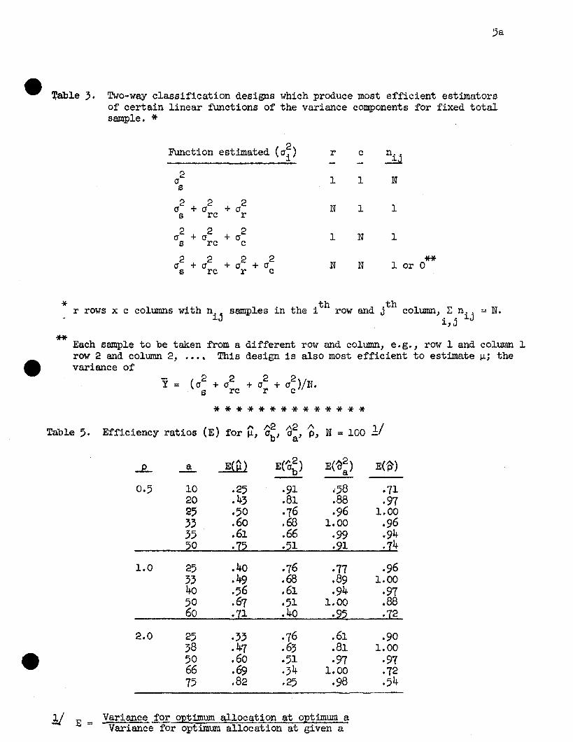
e ~able 3. Two-way classification designs which produce most efficient estimatorsof certain linear functions of the variance components for fixed totalsample. *

Function estimated (cr~) r c nijl.

21 1 Ncr

s2 2

+ cr; N 1 1cr + crs rc

2 + (J2

+ a~ 1 N 1crs rc

2 2 2 2 **cr + (j + a + a N N 1 or 0s rc r c

* 1 with l' th .th d .th 1 ~ Nr rows x c co umns nij samp es In e l. rowan J co umn, .~.nij = •l,J

** Each sample to be taken from a different row and column, e.g., row 1 and column 1row 2 and column 2, •••• This design is also most efficient to estimate ~; thevariance of

**************

Table 5. Efficiency ratios (E) for a, ~~, '(j;, 'P, N = 100 1:/

1.0

2.0

a E{P) E(1r~) E(~2) E(~)a

10 .25 ·91 .. 58 ·7120 .43 .81 .88 .9725 .50 ·76 .96 1.0033 .60 .68 1.00 .9635 .61 .66 .99 .9450 .15 .51 .91 .14

25 .40 .76 ·11 .9633 .49 .68 .89 1.0040 .56 .61 .94 .9750 .67 ·51 1.00 .8860 .11 .40 .95 .72

25 .33 ·76 .61 .9038 .47 .63 .81 1.0050 .60 -51 .97 .9766 .69 .34 1.00 ·7275 .82 .25 .98 .54

Y E= Variance for optimum allocation at optimum aVariance for optimum allocation at given a

The between-classes sum of squares can

6

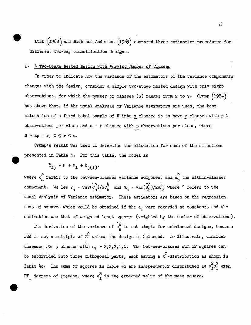
Bush (1962) and Bush and Anderson (1963) compared three estimation procedures for

different two-way classification designs.

2. A Two-Stage Nested Design with Varying Number of Classes

In order to indicate how the variance of the estimators of the variance component~;

changes with the design, consider a simple two-stage nested design with only eight

observations, for which the number of classes (a) ranges from 2 to 7. Crump (1954)

has shown that, if the usual Analysis of Variance estimators are used, the best

allocation of a fixed total sample of N into!:. classes is to have .£ classes with p+l

observations per class and a - r classes with p observations per class, where

N = ap + r, O:S r < a.

Crump~s result was used to determine the allocation for each of the situations

presented in Table 4. For this table, the model is

Yij = \..L + ai + bj(i)'

where O~ refers to the between-classes variance component and O~ the within-classes~2 4 ~2 4

component. We let Va = var(~a)/20b and Vb = var(~b)/20b' where" refers to the

usual Analysis of Variance estimator. These estimators are based on the regression

sums of squares which would be obtained if the a. were regarded as constants and the~

estimation was that of weighted least squares (weighted by the number of observations).

The derivation of the variance of ~2 is not simple for unbalanced designs, becausea

2SSA is not a multiple of X unless the design is balanced. To illustrate, consider

the case for 5 classes with n. = 2,2,2,1,1.~

be subdivided into three orthogonal parts, each haVing a X2-distribution as shown in

2 2Table 4c. The sums of squares in Table 4c are independently distributed as Xi0i with

DFi degrees of freedom, where ai is the expected value of the mean square.

6a

eTable 4a. Analysis of variance for two-stage nested design with 8 observations

(~ classes) --

Source of Degrees of Sum of Average value ofvariation Freedom (DF) squa"'~ mean square *

Between classes

vlithin classes

* 2, 2p .= (Ja! (JP. and k

a-I

8 - a,2= (64 - L:ni )/8(a-l).

/' . \ ';;',

SSA

SSB-~.._-.---

1'2 "'2 ( )/(Jb = MSBj O'a = MSA - MSB k.

;* * * * * * * * * * * * * *Table 4b. Values of Va and ~b for various designs; N =8, and for selected values of

p.**No. classes V for given p

**a:

(a) n. ....--- Vb1- .05 .1 .2 .5 1-..0 2.0 5.0 10.0

? Lt(?) ~/lQO, ·ill .~13 ·573 1.57 5.07 27·6 105 ·J.913 3U;),? ·.~1 .145 .128 .419 .993 2·90 14.8 54.9 .2004 2(4.) .163 .182 .226 ()96) -.8l2\ 2.15 10.1" 36.13 .250

_.J '--;----T-

5 ~C~J,~(2) .255 .274 .314 .467 .829 1.96 8.60 30.5 .3336 ~(2),l(4) .430 .447 .485 .623 ,941 1.90 7·43 25 .. 4 .5qo

7 ~,:I.(6). .937 .953 .988 1.11 1.40 2.22 6.83 2l.6 1.000- ~ ~:' t

* ("2)1 4 ~2 4V = Var ~a 2~bj Vv = _var(b)/~qb~ underlined values are minimum for givena2 2

p = 0' 1(Jb'a .

** Number in parentheses refers to number of classes with this n1

.

**************Table 4c. Subdivision of $SA for a = 5

Source

Among classes of~

Among classes of 1

Between two groups

Sum ofSquares

SSAl

SSA..... __ 2

SSl\3

DF

2

1

1

/1./)

Average value of '.

mean squares «(j~)2 2 '21-

( a,O -+ 20'aJ 0'::1.

/ 2 2, 2i O'b +(Ja j= 0'2

/ 2 ,2 2r. 0"1.. + 5';4 0' = (J~\ J;,I ,I. a':;

e Hence3

SSA = i: BSA. and k =[2(2) + 1 + 51€! /4 = 25/16.i=l J.

~; =(i: SSAi /(a-l) - MS~/k

7

""2var( a ) .1-....,4~a..... = [r. (DF)ia~/(a_l)2 + a~/3J/k2a~

2ab

_ 16 2 (7a~ g2, 2 2 169 4J 4- (25) 12 + 32 abG'a + 256 aa /ab

448 8 ~ 2= 1875 + a; p + b25 p

An examination of Table 4 reveals that the best experimental plan to estimate ia

varies from a = 2 to a = 7, depending on the value of p. This is the standard result

in designing experiments to estimate variance components; the criterion depends on the

values of the parameters to be estimated.2

Of course, the best plan to estimate ab is

e that for a = 1, for which Vb =1/2 = .143. Note that if p is small, one could do

qUite well in estimating for a; and a~ with small a. For p large, the best plan to

estimate a; is the worst to estimate a~. One other complication is that these

estimators are not ML unless the design is balanced. My students have been performing

some empirical sampling studies for p = 4 which indicate tentatively that the ML

estimator is superior (on a Mean Square Error basis) to the above weighted analysis of

variance estimator. I am not able to state whether this will continue to be true as

more samples are collected or for other values of p.

I should indicate that Crump showed that the optimal number of classes to estimate

"a; (using the usual analysis of variance) is approximately

al = N(Np + 2)/ ~(P+l) + 1.1 ·

Since al

, in general, will not be an integer, it appears that theelosest integer to~

~ should suffice because the variance profile is. quite flat in the neighborhood of

the optimum, except tha.t one should use a balanced plan if possible.

8

In general, one

does not lose much by using a. balanced plan unless p is quite large, and in many

situations the balanced plan is best.

All of these conclusions are based on the assumption that one has a good guess of

the value of p beforehand, that the analysis of variance estimator is to be used, and

that prime interest is centered on estimating 02•a

In Table 5, I have presented efficiency ratios (using the analysis of variance

2 2 2 2procedures) for estimating each of four parameters, fJ., O'b' O'a and p = O'a/O'b for N=lOO

and various values of p and number of classes. In the interest of time, I will not

dwell on these results; however, one can see that there is considerable loss in

efficiency in estimating one parameter if efforts are made to optimize the estimation

of some other parameter. Crump shows the effects of incorrectly guessing the value

of p on the efficiency of estimates of 0'2.a

1/2 < plPO < 2,

In generaJ., if

where Po is the guessed P, the loss in efficiency is less than 10%; this percentage

loss decreases as p increases.

The problem of needing a prior estimate of P in order to select an optimum design

is now being considered by one of my graduate students; a brief report on this

research will be made at the end of this paper.

3. Problem of Reducing Total Variability for a Two-Stage Production Process

Prairie ~961,196~ considered the problem of the effect of different designs in

estimating the variance components needed to allocate funds in the most efficient

manner to reduce the total product variance, 0'2 = 0'; + o~. Most of the theoretical

results are presented in Table 6. D units are assumed available to reduce 02;

e D = Da + Db' where Da units are to be spent to reduce 0'; and ~ units to reduce O'~,

l3a

if D = D ,a;

-k D21 + pe

=12

G.R

Fo~ulas used in Prairie's problem of reducing total variability for a t~stage production process

.- -k D1

e + P

e-kl(D-Da ) + pe-k2Da ; if 0 < D < D- a-(6.1)

'rable 6.

-l';.lDA

=: e + P .L ~ P ~ PI,

r 21~ '"-kl(D-C1 ) }';.1/C2

(6.2) oR p:: VO(p~ = = e p

-k2C1 -k2/C2 '"+ pe S- o

PI ~ p :5 P2,-k D

1 + pe 2 '"::: . p ~ P2,

(6.3) ~"~-: " ~ [(a-hlSE -1Jwhere K :: [N(N~2l?-1) + al?(l?+l)] /N(a-l) and

Q:: o~ ~\l + (l?+l)P] X(r_l) + ~ + l?Pj X(a_r_l) + Cl + ap(l?+l)P/~X(l'~ l-.

(6.4) p = Prob [Vo(p) ~ t3J'where t3 is a fixed number between min Vo and max VO'

(9 min Vo + max VO)/IO j

(3 min Vo + max VO)/ 4 .

9

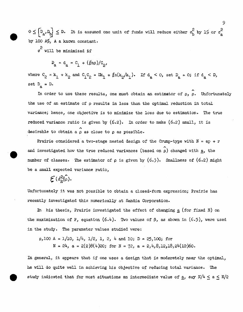
o ~ [Da'~ ~ D. It is assumed one unit of funds will reduce either O'~ by 1% or 0';by 100 A%, A a known constant.

20' will be minimized if

where C2 =kl + k2 and CI C2 = Dkl + [n(k2/kl ). If da < 0, set Da = OJ if da < D,

set D = D.a

In order to use these results, one must obtain an estimator of p, p. Unfortunately

the use of an estimate of p results in less than the optimal reduction in total

variancej hence, one objective is to minimize the loss due to estimation. The true

reduced variance ratio is given by (6.2). In order to make (6.2) small, it is

desirable to obtain a p as close to p as possible.

Prairie considered a two-stage nested design of the Crump-type with N = ap + r

"and investigated how the true reduced variances (based on p) changed with a, the

number of classes. The estimator of p is given by (6.3). Smallness of (6.2) might

be a small expected variance ratio,

2'"~(dRlp).

Unfortunately it was not possible to obtain a closed-form expressionj Prairie has

recently investigated this numerically at Sandia Corporation.

In his thesis, Prairie investigated the effect of changing ~ (for fixed N) on

the maximization of P, equation (6.4). Two values of ~, as shown in (6.5), were used

in the study. The parameter values studied were:

p,lOO A = 1/10, 1/4, 1/2, 1, 2, 4 and 10; D = 25,100; for

N = 24, a = 2(2)8(4)20; for N = 72, a = 2,4,8,12,18,24(12-)60.

In general, it appears that if one uses a design that is moderately near the optimal,

he will do qUite well in achieving his objective of reducing total variance. The

study indicated that for most situations an intermediate value of ~, say N/4 :s a :s N/2

will give almost optimal results.

be a =N/3.

10

If one value of ! were to be recommended, it would

P was computed by use of Incomplete l3eta approximations. Profiles of VO(~) are

given in the two Prairie references.

4. Extensions to Multi-Stage Production Processes

In the five-stage nested experiment mentioned earlier, I had proposed a so-called

staggered design. This design was constructed to eqUalize (as far as possible) the

degrees of freedom for the various parts of the analysis of variance. Prairie (1962)

also considered my staggered (Dl ) design plus other non-balanced three-stage nested

designs.. with the modeli=l,2, ••• ,aj=l,2, ••• ,b

ik=l,2, ••• ,nij

Some of these are presented in Table 1, plus a balanced design, for N = 48. vlhen

he was a graduate student at Raleigh, L. D. Calvin became interested in these non-

balanced designs. He has subsequently used some of them; see Calvin and Miller

(1961). Prairie developed a specific procedure for constructing his three-stage

designs, called D2-designs:

1) N = aql + r l , 0 S r l < a.

Assign ql + 1 units to each of r l A-classes (designated as group Gl ) and

ql units to each of a-rl A-classes (designated as group G2 )·

2) b =a~ + r 2, 0 S r 2 < a.

To each A-class assign ~ B-classes and then one extra B-class to each of

r 2 A-classes. Make sure that b > a.

lOa

*Table 7. Some three-stage nested designs with N = 48 observations.

Balanced D.F. (15, 16, 16)

16

In

Calvin-Miller and

Prairie (D2)Balanced Staggered (Dl )

A

rS7-1 n!?/A

C/B/A12 8 8

Other Prairie designs, unbalanced D.F.

-±-. +(23, 16, 8) r I

8 16

(15, 24, 8)r

8 8

(7,52,8) 1-1, +t +18

Special staggered (11.) design for (15, 24, 8)

l-S I~ +- +4 4

++8

* The number below each basic plan is the number of replications used for the completeexperiment. The degrees of freedom (D.F.) are between A-classes, B in A classesand C in B in A classes, respectively.

lOb

e ,+,ab1e 7a. Some Non-Balanced Four and Five-stage Nested Designs

Bainbridge (Calvin-Miller) designs

Four stages Five stages

1;\1 = 4

nij = .3,1

nijk = 2,1,1~

I ISome Prairie deSignS:

ni = 5nij = .3,2nijk = 2,1,2

nijk!= 2,1,1;11,1,2II . f

Five stases

ni = 4

nij =nijk=

Four stages

*Anderson five-stage staggered design

n+t+¥+ tl

+ta2 ni =16,8,4,2,1 a,; a4 a5

nij = 8,4,2,1,.1

nijk = 4,2,1,1,1

nijkf = 2,1,1,1,1

* ai replications of each basic plan plus ~ replications of the full design given

at the top of Table 1, giving i~lai A-samples. This design is given in Anderson

and Bancroft (1952) with 13.1=2, a2=2, a,;=4, a4=8, a5=O.

,

11

3) 'Vlithin each A-class" assign the observations (nij ) to the B-classes as equall:y

as possible.

When b ::: N/2" the D2-design will usually satisfy the relations:

Ini - ntl = 0 or 1 ;

Inij - ntml =0 or 1.

Consider the four D2-designs given in Table 7. In all cases" the ni are equal

for a given design; the nij are either 2 or 1. ~ staggered (D1 ) design does not

have these features" e.g., ni =2 and 4" nij =1 and 2. An additional benefit to be

derived from a design such as the D2

(15,,16,,16) design is the facility to detect

variance heterogene1ty. If we indicate the three observations for a given A-class

as x11,x12 and x21, then a single degree of freedom contribution to SSC is

(x11 - x12'f/2. This can be computed separately for each of the 16 A-classes and

tested for heterogeneity; if the A-classes are sampled on successive time periods"

one could determine if there was a time trend in the variance estimates. The same

procedure can be used with SSB" where the single-degree-of-freedom contribution is

(xU + x12 - 2x21 )2/6• For my staggered (&1) design" six observations must be

secured at each step" giving two degrees of freedom for C and B at each step but

with only 8 steps instead of 16.

For each of 14 non-balanced designs, Prairie computed the efficiency ratios

Ea, ~, and Ec" where

E = var(~) for a given non·ba1anced design

'1("'2)var ~i for the balanced design

assuming the analysis of variance estimation procedure of Table 8. The design

parameters considered were Pl = 02

/02 and P2 = 0b2/02 =1/10,1/4,1/2,,1,2,4,10.a cc

Special analyses for my staggered (D1 ) design and the Calvin-Miller (D2) design

are presented in Table 9.

12

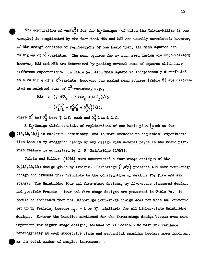
e !ale computation of var(o~) for the D2

-designs (of which the Calvin-Miller is one

example) is complicated by the fact that MBA and MSB are usually correlated; however,

if the design consists of replications of one basic plan, all mean squares are2 .

multiples of X -variates. The mean squares for rrr:y staggered design are uncorrelated;

however, MBA and MSB are determined by pooling several sums of squares which have

different expectations. In Table 9a, each mean square is independently distributed

as a multiple ofax2-variate; however, the pooled mean squares (Table 8) are distrib­

uted as weighted sums of X2-variates, e.S. ,

MBA = (7~ + 7 MBA2 + MBA,)!15

( 22 ..22 22;= Xlol + x202 + X,o,) 15,

-~ 2 2where x;: and X2 have 7 d. f. each and X; has 1 d. f •

A D2-design which consists of replications of one basic plan ~UCh as for

e (15,16,16») 1s. easier to administe~ and is more amenable to sequential experimenta­

tion than is my staggered design or any design with several parts in the basic plan.

This feature is emphasized by T. R. Bainbridge (1965).

Calvin and Miller (1961) have constructed a four-stage analogue of the

D2(15,16,16) design given by Prairie. Bainbridge (1965) presents the same four-stage

design and extends this principle to the construction of designs for five and six

stages. The Bainbridge four and five-stage designs, my five-stage staggered design,

and possible Prairie four and five-stage designs are presented in Table 7a. It

should be indicated that the Bainbridge four-stage design does not meet the criteria

set up by Prairie, because nij = 1 or';, similarly for all higher-stage Bainbridge

designs. However the benefits mentioned for the three..stage design become even more

important for higher stage designs, because it is possible to teat for variance

heterogeneity at each successive stage and sequential sampling becomes more important

e as the total number of samples increases.

Table 8. Analysis of variance for general three-stage nested design

l2a

Among C- classes in B in A N-b

Source of variation

.Among A-classes

Among B-classes in A

Mean.m:.. Square

a-l MSA

b-a MSB

MSC

Average value ofMean Square

2 I 2 2°c + K10b + K20a

2 20c + Klcrb

O~

A2oc

IS. = [N - ~; (~/ni>]/(b-a) ;

Ki = r~ ~ (nij/ni ) - Ei~ (n~j)/~/(a-l)

b J J

K2 =[N - t ni/N]/(a-l) •

MaB - MaC 1'2 K1MSA - KiMSB - (Kl - Ki) MSC. ° =Kl ~ a K1K2

**************Table 9a. Analysis of variance for the staggerea (Di) ~design in Table 7

Source of variation D.F. M.S. Average value of M. S.-Al (Group 1) 2 2 2 2

7 MBAl 0c + 2crb + 4cra = 0'1

A2 (Group 2) 7 MSA22 2 2 2

crc + crb + 20 ::.:: O2.a

A3

(Between Groups) 1 MSA3 O~ + 4/3 O"~ + 8/3

2 20"a ::.:: 0'3

Bl (Group 1) 8 MSB2 2

1 O'e + 20'b

B2 (Group 2) 8 MSB22 2

0c + °b

C (Group 1) 16 MaC 20"

C

Table 9b. Analysis of variance for the Calvin-Miller ( D2 ) design in Table 7

Source of variation ~ M.S. Average value of M.S.

A 15 MSA 2/2 20"c + 5 3 O"b + 3cra

16 2/ 2B MSB O'c+ 43 Ob

C 16 MSC2

O'c

13

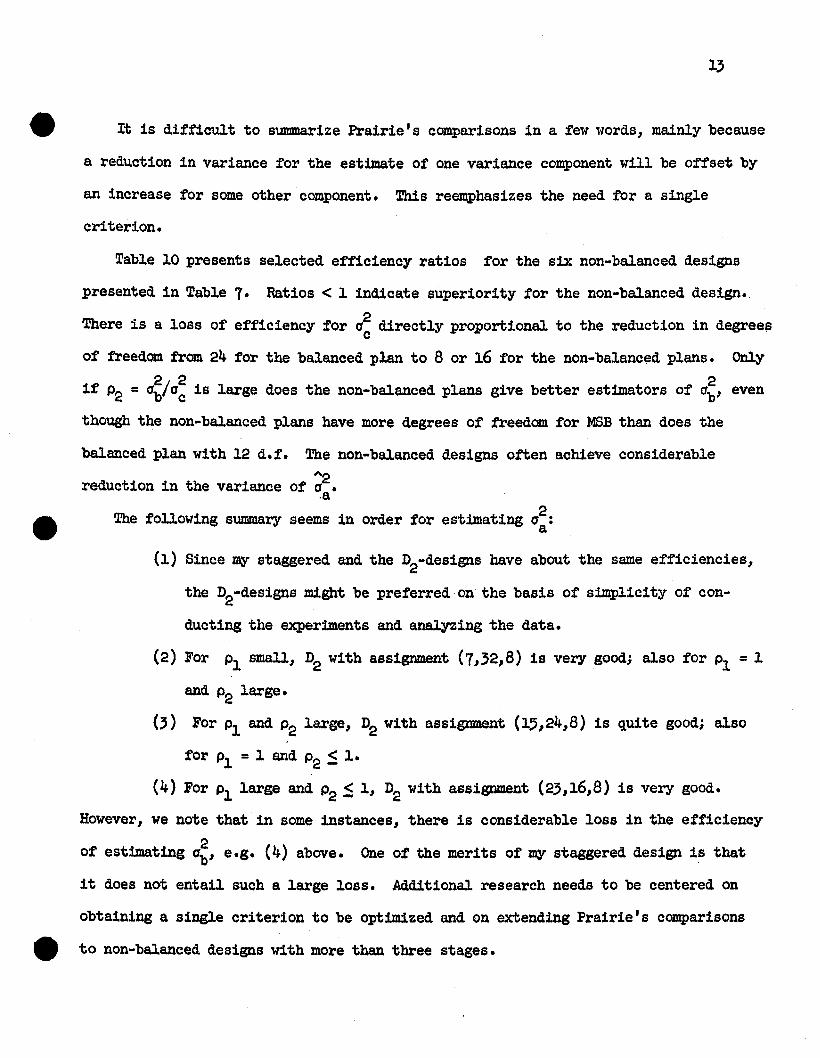
e It is difficult to summarize Prairie's comparisons in a few words, mainly because

a reduction in variance for the estimate of one variance component will be offset by

an increase for some other component. This reemphasizes the need for a single

criterion.

Table 10 presents selected efficiency ratios for the six non-balanced designs

presented in Table 7. Ratios < 1 indicate superiority for the non-balanced design.

There is a loss of efficiency for a2 directly proportional to the reduction in degreescof freedom from 24 for the balanced plan to 8 or 16 for the non-balanced plans. Only

2; 2 2if P2 =ab ac is large does the non-balanced plans give better estimators of ab, even

though the non-balanced plans have more degrees of freedom for MSB than does the

balanced plan with 12 d.f. The non-balanced designs often achieve considerable~2

reduction in the variance of a •·a

2e The following summary seems in order for estimating aa:

(1) Since m;y staggered and the D2-designs have about the same efficiencies,

the D2-designs might be preferred on the basis of simplicity of con­

ducting the experiments and analyzing the data.

(2) For Pl small" D2 with assignment (7,32,8) is very good; also for Pl = 1.

and P2 large.

(3) For P1. and P2 1.arge, D2 With assignment (1.5,,24,8) is quite good; also

for P1. =1 and P2 S 1..

(4) For P1. 1.arge and P2 S 1." D2 with assignment (23,,1.6,8) is very good.

However, we note that in some instances, there is considerable 1.oss in the efficiency

2of estimating ab, e.g. (4) above. One of the merits of my staggered design is that

it does not entaU such a 1.arge loss. Additional research needs to be centered on

obtaining a single criterion to be optimized and on extending Prairie's comparisons

e to non-balanced designs with more than three stages.

l3a

Table 10. Selected efficiency ratios for comparing the non-balanced designs with thebalanced desiGn in Table 8*

Values of EDesign for P;L eq,ua~ to

~ EP2 D.F. ~ ...1!!± 1 4 c

- -1/4 (15,16,16) D1 1.02 .89 .83 ~ 1·50

(15,16,16) D2 1.15 .89 ·77 1.71 1.50(15,24,8) D1 .88 .84 .82 2·50 3·00(15,24,8) D2 ·92 .82 .76 2·72 3.00(23,16,8 ) D2 1.77 .91 ill 3.89 3.00(7,32,8 ) D2 ill 1.17 1.46 2.27 3·00

1 (15,16,16) D1 ·93 .88 .83 1.05 1.50(15,16,16) D2 1.03 .91 ·79 1.15 1.50(15,24,8 ) D1 .69 ·75 ·79 1.21 3.00(15,24,8) D2 ·72 ill ·74 1.27 3.00(23,16,8 ) D2 1.48 .99 .61 1.89 3.00(7,32,8 ) D2 .46 .86 1.31 1.02 3·00-

4 (15,16,16) D1 .86 .85 .83 .88 1.50(15,16,16) D2 ·91 .88 .82 .85 1.50(15,24,8 ) D1 ·55 .60 ·70 .67 3.00(15,24,8) D2 .57 .61 .:.E§ !65 . 3.00(23,16,8 ) D2 1.25 1.08 ·75 .99 3·00(7,32,8 ) D2 .28 .d§ .93 ill 3.00

*A Minimum values for given (P1'P2) underlined.

14

5· Comparisons of Estimators and DeSignS for Two-~lay Classification Operations

Three unbiased methods for estimating variance components were compared for a

two-way classification operation by Bush (1962) and subsequently published in~­

nometrics in 1963. Two of the procedures, A and B, are based on the respective

methods of fitting constants and weighted squares of means described by Yates (19,4)

for fixed effects models. The third procedure, H, which uses unadjusted sums of

squares" was developed by Henderson (1953) explicitly for random models. Bush con-

sidered only connected designs. The three procedures were compared on the bas1s of

variances of estimated variance components for a number of experimental designs and

parameter values (papulation variance components ) with the aid of a UNIVAC 1105

computer. For each estimating procedure, efficiency factors relative to a balanced

design were computed for the various non-balanced designs considered.

The model considered for occupied cells 1mS

i =l,2, ••• ,a; j =l,2, ••• ,b; k =1,2, ••• ,n1j

Bush based his results on the cell means,

•

- '"Yij • = ~ij =~ + r i + c j + (rc)ij + eij•

222 2The variance components were 0 , 0 , 0 and o. Eighteen sets of parameter valuesr c rc e

were used by Bush (1962): 0; ranged from 1/2 to 16, a: from 0 to 16, o~ from 0 to

16 and 02

= 1; four sets are presented in the 'rechnometrics article.·e

Insufficient computer storage prevented our investigating larger than 6 x 6

designs; extensions to desisns with more rows and columns are planned in the future.

Six non-balanced and one balanced 6 x 6 designs are presented in Table 11.

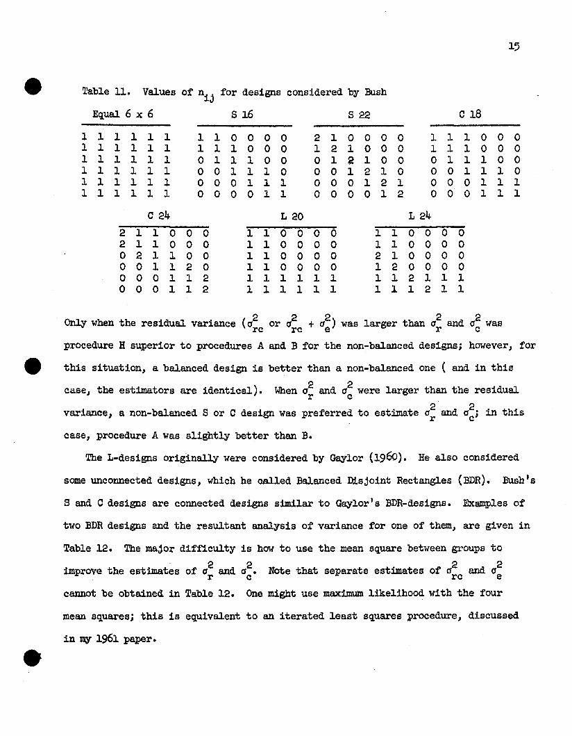
15

Table 11- Values of nij for designs considered by Bush

Equal 6 x 6 S 16 S 22 C 18

1 1 1 1 1 1 1 1 0 0 0 0 2 1 0 0 0 0 1 1 1 0 0 01 1 1 1 1 1 1 1 1 0 0 0 1 2 1 0 0 0 1 1 1 0 0 01 1 1 1 1 1 0 1 1 1 0 0 0 1 2 1 0 0 0 1 1 1 0 01 1 1 1 1 1 0 0 1 1 1 0 0 0 1 2 1 0 0 0 1 1 1 01 1 1 1 1 1 0 0 0 1 1 1 0 0 0 1 2 1 0 0 0 1 1 11 1 1 1 1 1 0 0 0 0 1 1 0 0 0 0 1 2 0 0 0 1 1 1

C 24 L 20 L 24

2 1 1 0 0 0 1 1 0 0 0 0 1 1 0 0 0 02 1 1 0 0 0 1 1 0 0 0 0 1 1 0 0 0 00 2 1 1 0 0 1 1 0 0 0 0 2 1 0 0 0 00 0 1 1 2 0 1 1 0 0 0 0 1 2 0 0 0 00 0 0 1 1 2 1 1 1 1 1 1 1 1 2 1 1 10 0 0 1 1 2 1 1 1 1 1 1 1 1 1 2 1 1

Only when the residual variance (a;c or a;c 222+ ae) was larger than ar and ac was

procedure H superior to procedures A and B for the non~balanced designs; however, for

this situation, a balanced design is better than a non-balanced one ( and in this

case, the estimators are identical). ~fuen 0'2 and 0'2 were larger than the residualr c

variance, a non-balanced S or C design was preferred to estilllate 0'2 and 0'2; in thisr c

case, procedure A was slightly better than B.

The L-designs originally were considered by Gaylor (1960). He also considered

some unconnected designs, which he Galled Balanced Disjoint Rectangles (BDR). Bush •s

S and C designs are connected designs s1m1lar to Gaylor IS BDR-designs. Examples of

two BDR designs and the resultant analysis of variance for one of them, are given in

Table 12. The major difficulty is how to use the mean square between groups to

2 2 . 2 2improve the estilllates of ar and ac. Note that separate estmates of arc and ae

cannot be obtained in Table 12. One might use maximum likelihood with the four

mean squares; this is equivalent to an iterated least squares procedure, discussed

in my 1961 paper.

15a

Table 12. Some balanced disjount rectangle designs and the analysis of variance

1 1 1 0001 1 1 0001 1 1 0 0 0o 0 011 1o 001 1 1o 001 1 1

.)

1 11 1

o

o

o

o1 11 1

o

o

o

o1 11 1

o

o

o

o1 11 1

Analysis of variance for second design

squaremeanAverage value of

MSR

MSC

MSC

MeanSquares

MSGD.F.3

4

4

4

Columns in Groups

Rows in Groups

Source of variationBetween Groups

(R x C) in Groups

2 2° + °e rc

2 2°e + °rc2 2

C1 + 0e rc2 2

0+0e rc

**************Table 13. Efficiency of some two-waY aesigns for est:l.fuating 0; and Pr , :N' = 30 *

1.0

r

35678

10111415

c

106554

3332

s

ooo2

6

o82o

E(~2)r

.69

.951.00

.981'.00

'.88.90.96

1.00

E(Pr )

.74

.981.00

.95

.94

1.00·97.83.84

4.0

r

10121519

10152024

c

3322

3222

s

o6o

11

oo

106

E(~2)r

·74.82'.97

1~00

·59.84.94

1.00

E(Pr )

1.00·97·93.63

l'.00·99·53

* r =no. rows; c = no. columns; N =rc if s = 0; N = r(c-1) + s if s > O.

16

e Gaylor considered the problem of optimal designs to estimate a2 • It was shownr

first that if the design were restricted to a class of designs in which nij = 0 or

n (. n integer), n should equal one. Hence each cell would either be empty or contain

e 2 222only one observation. In this case, only a", a and. a = a + a could be estimated.r c e rc

Using Method A (fitting constants), we came up with the following rule (see my 1961

paper, p. 811):

1) If Pr >~ use one column with r = N - r' rows and a second column

with r' of these rows, where r' is the integer (~ 2) which is closest

to 1 + (N - 2)/P 12.r

2) When Pr s{2, use a balanced design with the number of columns, c as the

integer closest to

Pr{N - 1/2) + N + 1/2. PrtN'- 1/2) + 2

In general, N/c will not be an integer; hence it probably would be

adVisable to use a few more or less observations to obtain balance.

Efficiency factors for some designs used to estimate a2 and P = a2/a2 are presentedr r r

in Table 13. Gaylor showed that the loss of efficiency due to the use of the incorrect

Pr is of the same order of magnitude as found by CI'\lD1P. If only a2 or P is ofc c

interest, interchange r and c in the above results.

The results in Table 13 show that if one wants to obtain good estimates of both2 . 2 . 2

<1r and <1c' he must alter the design, because an optimal design for ar furnishes little

information on a2 (note the small number of columns used). This led to Gaylor'sc2

investigation of the L-design, which consists of a good design for or superimposed on

a good design for 02• The diagonalized designs (8, C or BDR) have the same principlec

With sequences of balanced designs. Unfortunately no optimal rule for the formation

~ of such designs has been developed.

17

~ Computational procedures for non-balanced multi-factor designs may be very compli-

cated. Research on best estimators and designs is being planned.

6. Two-stage Nested Desisn with Composited Samples

In cases where the measurements cost is high, it may be advantageous to com,posite

some of the samples and take measurements on the com,posited samples. This may be

the case for sampling of many bulk materials, especially those involving chemical

assays. One of my graduate students, K. L. Kussmaul, is considering a two-stage

sampling problem with compositing of samples within the first-stage (A) classes. The

model for the composited measurement will be:

1 nij= .... + a + - 1: b ( )i nij k=l k i

)"i=1,2, ••• ,a

13=1,2, •.• ,ri

th thwhere nij samples are com,posited for the j measurement of the i A-class. As

before) ~ nij =ni and ~ ~ nij = Ni in addition, we assume the total number of

measurements is R =1: r i •i

Four procedures to estimate the variance components a; and a~ are being studied:

(1) Method of Weighted Means. Weights are proportional to the number of samples

com,posited per measurement.

S~ = 1: .1.1-£ nij yij12

- j ~ 1; nij yij12

i ni _j ~ G. j ~

Sfll\ = g niJ i'fj - ~ ~ [~ niJ lit

Analysis of Variance

Source ofVariation l2.:!.:. !1&.

A a-l MBAl

B in A R-a MSBl

18

The estimators are:

'" - "'2~l= ~ ~ nij Yi/N i ~bl = MSBI ;

"'2~al = (MSAI - MSBI )/kl '

(2) Method of Unweighted Class Means. Each A-class mean (Yh

) is given equal weight

for SSA2, where Yi • = ~(nij Yij)/ni i hence,

!"'2 1II J2 ~l J2 1~ nij Yij12S~ = ~ Yj:. - a~ Yi • e ~ Lni ; nij Yi~ - a ~ ; ni J ·

2 2 1 1The expected value of MSA2 = SSA2/(a-l) is <1a + k2C1b, where k 2 =a ~ ~

2 "'2same estimator of C1b is used as in (1), i.e., C1b2 = MS~. Hence

(} ) Method of Unweighted Measurements.

• ~e

s~ =

E(S~) =

1r-]2 lU _~2E - E Yij - R E E Yiji r i j i j

1 2 - 2 2 ~1 1 l]a2-(R - E r)<1 + E r. (- - -) -R i i a i j _ri R nij b

Again one would use MSBI to estimate C1~; hence,

'"Also ~}

t (1 1 1SSA.. - E r. - - ->:=­, i j r i R nij

19

(It.) Method of Maximum Likelihood. This method has been studied only for the case of

equal Dij and equal r i " when all estimation methods give identical results.

The evaluation of various compositing plans is based on minimiz1nB the variance

ot the estimated parameters sUbject to a fixed sampling cost, C =aCa + NCb + RCc'

where Ca" ~ and Cc are the respective unit A-class" B-class and measurement costs.

The usual difficulty faced here is that comparative variances of the three est.imators1' ....2"2 22

(J.1, O'al O'b) are functions ot P = O'a/abj in practice, one probably would make an

initial guess (po) and attempt to find compositing plans with high precision tor

values ot p in the neighborhood of p •o

A number of empirical studies have been madej some ot the results are presented

in Table 14. These studies indicate that the best compositing plan seems to be

balanced or nearly balancedj hence, there is little or no problem of selection of the

best estimator-, as indicated above.

It may be desirable, especially for very costly' measurements, to composite

samples from more than one A-class. Cameron (195l) discussed two such plans for

sampling to estimate the clean content of shipments of woolj one of these plans was

developed by Mr. Tanner, who is presenting a paper on composite samples at this Semi-

nar. At present, Mr. Kussmaul is considering some optimal sampling plans for these

more complicated compositing procedures.

19a

e ~able 14. 2 2Efficiencies of Various Compositing Plans in Estimating j.L, Ga and GbUsing Estimating Procedure (1) with Fixed Total Cost C* •

P = 4 p=l e =1/4

** i'r* ." E(~) E(~;) " E(~~) E(~;) " E(~) E(~;)aRN r 1 n1 E(j.L) E(j.L) E(Il)

!

C = 506 7 10 2,1(5) 2(4),1(2) 100 14 99 95 14 55 75 14 14

~ 8 8 2~3 ~,1(2~ 2Pl,1!2l 82 43 82 77 43 60 60 43 225 7 12 2 2 ,1(3 3 2 ,2 3 89 29 94 91 29 83 80 29 375 6 16 2,1(4) 4,3 4) 94 14 100 100 14 94 96 14 42

4810 2~4) 3(2l ,2(2j 72 57 72 74 57 71 66 57 414 7 14 2 3),1 4~2),3(2 75 43 77 81 43 86 80 43 61It 6 18 2(2),1(2) 5 2),4(2 77 29 80 86 29 95 91 29 76It 5 22 2 /1(3} 6(2},5(2 78 14 '1 89 14 - 100 100 14 79

-)

3. 8 12 3(2l ,2 4(3) 58 71 53 64 71 63 65 71 553. 7 16 3,2 2) 6,5(2) 58 57 54 67 57 70 74 57 72

e 3. 6 20 2(3) 7~2),6 59 43 55 69 43 75 81 43 863 5 24 2(2),1 8 3) 60 29 56 71 29 78 87 29 96.3 4 28 2,1(2) 10,9(2) 60 14 57 72 14 80 91 14 lOO

2 9 lO 5,4 5(2) 39 100 27 44 100 35 48 100 362 8 14 4(2) 7(2~ 40 86 28 46 86 38 55 86 482 7 18 4,3 9(2 40 71 2$ 48 71 41 60 71 gz2 6 22 3(2) 1l(2j 40 57 29 49 57 42 64 572526 3... 2 13~2 40 43 29 49 43 43 66 43 69a 430 2(2) 152 40 29 29 50 29 44 68 29 74a 3 34 2,1 17(2) 40 14 29 50 14 45 70 14 76

C = 4848 8 2(4} 2(4) 73 57 10 11 51 62 58 57 303618 2(3) 6(3) 59 43 55 68 43 73 18 43 78

* C =aC + N~ + RC , where C =2, ~ =1E =relative efficiency as percentage. a c a

and Cc = 4; a A-classes, N =Eni samples and R =Eri composites (measurements),

2/ 2P =Ga Gb •.** 1(5) indicates 1,1,1,1,1; etc.

e

20

7· Bayesian Estimation of Variance Components in a Two-step Estimation Process forTwo-stage Nested DeSignS

We are now considering a simplified model for a two-stage nested design,

Yijk =ai + b~(i)' i =1,2, ••• ,a; j =l,2, ••• ,ni '

where it is assumed that ~ is zero (or if known to be,some other value, the observa-

tions are coded so that the new mean is zero). This assumption may not be too

unrealistic in many processes, and where it is not true the approximation of sub­

tracting the sampJ.e mean should not seriously affect the results. The analysis of

variance will now have.! degrees of freedom for MBA, and the expected value of MBA

2 2 ""2is 0b + Na la. Hence 0 =a(MSA • MBB)/N. The optimal allocation of degrees ofa .a

freedom (a,N-a) to 'minimize the variance ot ~ i6 g:Lven by the equation

02

a arr.:a=P="2 •

°b

(1)

(2)

A. I. Weiss is investigating a two-stage procedure:

Nl « N) observations are observed first with al h-classes, say, ~ = Nl/2.

From these are obtained MBAl and MB~, based on al and Nl - ta:J.. degrees O'i free-

'"dom, respectively, and Pl =~(MBAl - MSBl )/Nl (MSB1 )·

The degrees of freedom (a2 and N2

- a2 =N - Nl - a2) for a second step are

then allocated as follows to minimize the variance of the combined estimator

of 02 :a

a2 N2 "'. N2 '"=-NP=-N P •N-al -a2

The combined estimator of p is"" .~c =(~+ a2 )(MSAc - MSBc)/N(MSBc )'

where MSAc = (SSAl + SSA2)/(al + a2), and MSBc = (SS~ + SSB2 )/(N-al -a2), SSA2

and SSB2 obtained in the second step.

21

e Of course, the second step allocation is still only a guess, but is based on experi­

mental evidence.

Since the above results involve guesses for p, one naturally considers the use

2of prior distributions for p, and collaterally, Bayesian estimates of aa' In order

to make the mathematics tractable, Weiss is using Gamma-function priors, e.g.

The prior for p is

O<p<oo.g(p) £( )

P+q-2r l + r 2 + r1kp

tit Weiss conceives of the prior distribution being based on a hypothetical experi-

•E(p) =.,=

ment, from which we obtain r l = SSBO and r 2 = SSAo. In order to have a finite second

moment for g(p), the smallest values of p and q are 2 and 4, respectively. For p = 2

and q = 4,

This "minimum-information" prior distribution is the same as a posterior distribution

based on 6 d.f. for SSAO and 2 d.f. for SSBO' coupled with a non-informative prior

(p =q = 1; r l = r 2 =0).

Weiss concentrated his

neighborhood of p =1, i.e.,

attention on obtaining good estimators of a; in the

2 2aa = ab; then he studied the robustness of various

procedures when p deviates from 1, e.g., p =1/10, 1/4, 1/2, 2, 4 and 10. For a

standard, he used the usual one-step experiment with N/2 A-classes (and hence N/2 d.f.

for both SSA and SSB), so that k = 2.

22

For all two-step procedures, the first step had Nl /2 degrees of freedom for

both S~ and SSD1, i.e., al/(N1-al )=1 and k = 2. If priors were used, various

procedures were introduced to determine the ratio of r 2 to r l • In addition to

Procedure A, the non-informative prior mentioned above, three minimum information

priors were considered:

Prior based on E(p2) =1.

1\2aa at the first step is

B. The allocation to minimize the variance ofal • r:::-2':

Nl

- al

=VE(p ), = lj r 2/rl =1.

Naturally this allocation does not minimize the variance of the combined

estimator of a:.c. Prior based on E(p) =1. This tends to concentrate information near

p =lj r 2/rl =3·

D. Prior based on ~o = (MSAO - MSBo)/2MSBo = 1. This returns to the concept

of a previous hypothetical eJqleriment, with the estimator concentrated

near lj r 2/rl = 9.

These priors require further specification, because MSAO and MSBo are unknown. Weiss

recommends estinnting them from the first step.

Allocation at the second step for B, C and D would be based on the optimal

allocationa2 N2~2

No = -N E(p) ,-al -a2

where E(p2) is determined from the posterior distributions obtained after the first

step. After the second step is completed, final posterior distributions were used

to obtain the estimates of a2• Since this estimation procedure was quite complicated,a

empirical sampling procedures were used to determine the efficiency relative to the

one-step standard procedure. These results for N =100 are presented in Table 15;

other results for N = 25 and 50 are also available. Some one-step prior procedures

e are includedj these are indicated by Nl = 100.

23

Table 15. Percent Reduction in Mean Square Error of Two-Stepand Prior procedur.

7es over One-Step Standard Pro­

cedure, N = lOa.!

p

Prior N1 1/10 1/4 1/P. 1 4 10

None 10 25 - 3 -30 -40 -19 9 30None 20 38 17 -14 -20 - 4 18 28None 40 35 '14 - 4 - 7 2 12 24

A 10 -100 -60 -30 -29 -15 8 2720 10 7 -13 -12 - 6 12 2140 44 36 8 - 2 - 8 5 5

B lO 52 51 20 4 0 7 440 74 57 16 3 15 2 - 2

100 56 51 26 0 10 - 2 3

c 40 40 43 14 10 19 15 14100 34 36 21 9 5 5 5

D 40 - 3 16 - 8 1 10 16' 22

!/ Negative results indicate the standard procedure issuperior; procedures using no prior are unbiased, i.e.,mean square error equals variance. Additional samplingis being conducted.

If no prior is used, N1 = 40 is recommended, because at worst it is only 6%

less efficient than the one-step plan (p=l) and is almost as efficient as N1 = 20

for large or small p. Of the priors, C in two-steps is recommendedj in aeaeral

this shows considerable imporvement over the no-prior two-step procedure, especially

for p between 1/2 and 2. As indicated in .Tab1e 15, further sampling is being conducted.

REFERENCES

Anderson, R. L. 1961. Designs for estimating variance components. Proc. Seventh

Conf. Des. Expts. Army Res., Dev., Test., ARODR 62-2, 781-823. Inst. of Stat.

Mimeo Series No. 310.

Anderson, R. L. and T. A. Bancroft. 1952. Statistical Theo;g in Research. McGraw­

Hill, New York.

Bainbridge, T. R. 1965. Staggered, nested designs for estimating variance components.

~dustrial Quality Control 22(1):12-20.Bush, N. 1962. Estimating variance components in a multi-way classification. UnpUb­

lished Pil.D. Thesis, North Carolina State University, Raleigh. Inst. of stat.

M1meo Series No. 324.

Bush, N. and R. L. Anderson. 1963. A comparison of three different procedures for

estimating variance components. Technometrics 5:421-440.Calvin, L. D. and J. D. Miller. 1961. A sampling design with incomplete dichotomy.

!\gron. J. 53:325-328.Cameron, J. M. 1951. The use of components of variance in preparing schedules for

sampling of baled wool. Biometrics 7(1):83-96.Crump, P. P. 1954. Optimal designs to estimate the parameters of a variance compo­

nent model. Unpublished Ph.D. Thesis, North Carolina state University, Raleigh.

Gaylor, D. W. 1960. The construction and evaluation of some designs for the esti­

mation of parameters in random models. Unpublished Ph.D. Thesis, North Carolina

State University, Raleigh. Inst. of stat. Mimeo Series No. 256.

Henderson, C. R. 1953. Estimation of variance and covariance components. Biometrics

9:226-252.

Newton, R. G., M. vi. Philpott, H. F. Smith and W. G. Wren. 1951. Variability of

Malayan rubber. Indus. and gr. Chem. 43 :329.

Prairie, R. R. 1961. Some results concerning the reduction of product variability

through the use of variance components. Proc. Seventh Coni'. Des. Expts. Army

Res., Dev., Test., ARODR 62-2, 655-688.

Prairie, R. R. 1962. Optimal designs to estimate variance components and to reduce

product variability for nested classifica.tions. Unpublished Ph.D. Thesis,

North Carolina State University, Raleigh. Inst. of Stat. Mimeo Series No. 313.

Yates, F. 1934. The analysis of multiple classifications with unequal numbers in

the different classes. J. lmJ.. Stat. Ass. 29:51-66.