Non-Asymptotic Analysis of StochasticApproximation Algorithms for Machine Learning

Francis BachINRIA - Sierra Project-team

Ecole Normale Superieure, Paris, Francefrancis.bach@ens.fr

Eric MoulinesLTCI

Telecom ParisTech, Paris, Franceeric.moulines@enst.fr

Abstract

We consider the minimization of a convex objective functiondefined on a Hilbert space,which is only available through unbiased estimates of its gradients. This problem in-cludes standard machine learning algorithms such as kernellogistic regression andleast-squares regression, and is commonly referred to as a stochastic approximationproblem in the operations research community. We provide a non-asymptotic anal-ysis of the convergence of two well-known algorithms, stochastic gradient descent(a.k.a. Robbins-Monro algorithm) as well as a simple modification where iterates areaveraged (a.k.a. Polyak-Ruppert averaging). Our analysissuggests that a learning rateproportional to the inverse of the number of iterations, while leading to the optimal con-vergence rate in the strongly convex case, is not robust to the lack of strong convexity orthe setting of the proportionality constant. This situation is remedied when using slowerdecays together with averaging, robustly leading to the optimal rate of convergence. Weillustrate our theoretical results with simulations on synthetic and standard datasets.

1 Introduction

The minimization of an objective function which is only available through unbiased estimates ofthe function values or its gradients is a key methodologicalproblem in many disciplines. Its anal-ysis has been attacked mainly in three communities: stochastic approximation [1, 2, 3, 4, 5, 6],optimization [7, 8], and machine learning [9, 10, 11, 12, 13,14, 15]. The main algorithms whichhave emerged are stochastic gradient descent (a.k.a. Robbins-Monro algorithm), as well as a simplemodification where iterates are averaged (a.k.a. Polyak-Ruppert averaging).

Traditional results from stochastic approximation rely onstrong convexity and asymptotic analysis,but have made clear that a learning rate proportional to the inverse of the number of iterations, whileleading to the optimal convergence rate in the strongly convex case, is not robust to the wrong settingof the proportionality constant. On the other hand, using slower decays together with averagingrobustly leads to optimal convergence behavior (both in terms of rates and constants) [4, 5].

The analysis from the convex optimization and machine learning literatures however has focusedon differences between strongly convex and non-strongly convex objectives, with learning rates androles of averaging being different in these two cases [11, 12, 13, 14, 15].

A key desirable behavior of an optimization method is to be adaptive to the hardness of the problem,and thus one would like a single algorithm to work in all situations, favorable ones such as stronglyconvex functions and unfavorable ones such as non-stronglyconvex functions. In this paper, weunify the two types of analysis and show that (1) a learning rate proportional to the inverse of thenumber of iterations is not suitable because it is not robustto the setting of the proportionalityconstant and the lack of strong convexity, (2) the use of averaging with slower decays allows (closeto) optimal rates inall situations.

More precisely, we make the following contributions:

− We provide a direct non-asymptotic analysis of stochastic gradient descent in a machine learn-ing context (observations of real random functions defined on a Hilbert space) that includes

1

kernel least-squares regression and logistic regression (see Section 2), with strong convexityassumptions (Section 3) and without (Section 4).

− We provide a non-asymptotic analysis of Polyak-Ruppert averaging [4, 5], with and withoutstrong convexity (Sections 3.3 and 4.2). In particular, we show that slower decays of thelearning rate,together with averaging, are crucial torobustlyobtain fast convergence rates.

− We illustrate our theoretical results through experimentson synthetic and non-synthetic exam-ples in Section 5.

Notation. We consider a Hilbert spaceH with a scalar product〈·, ·〉. We denote by‖ · ‖ theassociated norm and use the same notation for the operator norm on bounded linear operators fromH to H, defined as‖A‖ = sup‖x‖61 ‖Ax‖ (if H is a Euclidean space, then‖A‖ is the largestsingular value ofA). We also use the notation “w.p.1” to mean “with probability one”. We denotebyE the expectation or conditional expectation with respect tothe underlying probability space.

2 Problem set-up

We consider a sequence ofconvex differentiable randomfunctions(fn)n>1 from H to R. We con-sider the following recursion, starting fromθ0 ∈ H:

∀n > 1, θn = θn−1 − γnf′n(θn−1), (1)

where(γn)n>1 is a deterministic sequence of positive scalars, which we refer to as thelearningrate sequence. The functionfn is assumed to be differentiable (see, e.g., [16] for definitions andproperties of differentiability for functions defined on Hilbert spaces), and its gradient is an unbiasedestimate of the gradient of a certain functionf we wish to minimize:

(H1) Let (Fn)n>0 be an increasing family ofσ-fields. θ0 is F0-measurable, and for eachθ ∈ H,the random variablef ′

n(θ) is square-integrable,Fn-measurable and

∀θ ∈ H, ∀n > 1, E(f ′n(θ)|Fn−1) = f ′(θ), w.p.1. (2)

For an introduction to martingales,σ-fields, and conditional expectations, see, e.g., [17]. Note thatdepending whetherF0 is a trivial σ-field or not,θ0 may be random or not. Moreover, we couldrestrict Eq. (2) to be satisfied only forθn−1 andθ∗ (which is a global minimizer off ).

Given only the noisy gradientsf ′n(θn−1), the goal of stochastic approximation is to minimize the

functionf with respect toθ. Our assumptions include two usual situations, but also include manyothers (e.g., potentially, active learning):

− Stochastic approximation: in the so-called Robbins-Monro setting, for allθ ∈ H andn > 1,fn(θ) may be expressed asfn(θ) = f(θ)+〈εn, θ〉, where(εn)n>1 is a square-integrable mar-tingale difference (i.e., such thatE(εn|Fn−1) = 0), which corresponds to a noisy observationf ′(θn−1) + εn of the gradientf ′(θn−1).

− Learning from i.i.d. observations: for all θ ∈ H andn > 1, fn(θ) = ℓ(θ, zn) wherezn is ani.i.d. sequence of observations in a measurable spaceZ andℓ : H×Z is a loss function. Thenf(θ) is the generalization error of the predictor defined byθ. Classical examples are least-squares or logistic regression (linear or non-linear through kernel methods [18, 19]), wherefn(θ) =

12 (〈xn, θ〉 − yn)

2, or fn(θ) = log[1 + exp(−yn 〈xn, θ〉)], for xn ∈ H, andyn ∈ R

(or {−1, 1} for logistic regression).

Throughout this paper, unless otherwise stated, we assume that each functionfn is convex andsmooth, following the traditional definition of smoothness from the optimization literature, i.e.,Lipschitz-continuity of the gradients (see, e.g., [20]). However, we make two slightly differentassumptions:(H2) where the functionθ 7→ E(f ′

n(θ)|Fn−1) is Lipschitz-continuous in quadraticmean and a strengthening of this assumption,(H2’) in whichθ 7→ f ′

n(θ) is almost surely Lipschitz-continuous.

(H2) For eachn > 1, the functionfn is almost surely convex, differentiable, and:

∀n > 1, ∀θ1, θ2 ∈ H, E(‖f ′n(θ1)− f ′

n(θ2)‖2|Fn−1) 6 L2‖θ1 − θ2‖2 , w.p.1. (3)

(H2’) For eachn > 1, the functionfn is almost surely convex, differentiable with Lipschitz-continuous gradientf ′

n, with constantL, that is:

∀n > 1, ∀θ1, θ2 ∈ H, ‖f ′n(θ1)− f ′

n(θ2)‖ 6 L‖θ1 − θ2‖ , w.p.1. (4)

2

If fn is twice differentiable, this corresponds to having the operator norm of the Hessian operatorof fn bounded byL. For least-squares or logistic regression, if we assume that (E‖xn‖4)1/4 6

R for all n ∈ N, then we may takeL = R2 (or evenL = R2/4 for logistic regression) forassumption (H2), while for assumption(H2’), we need to have an almost sure bound‖xn‖ 6 R.

3 Strongly convex objectives

In this section, following [21], we make the additional assumption of strong convexity off , but notof all functionsfn (see [20] for definitions and properties of such functions):

(H3) The functionf is strongly convex with respect to the norm‖·‖, with convexity constantµ > 0.That is, for allθ1, θ2 ∈ H, f(θ1) > f(θ2) + 〈f ′(θ2), θ1 − θ2〉+ µ

2 ‖θ1 − θ2‖2.Note that(H3) simply needs to be satisfied forθ2 = θ∗ being the unique global minimizer off(such thatf ′(θ∗) = 0). In the context of machine learning (least-squares or logistic regression),assumption(H3) is satisfied as soon asµ2 ‖θ‖2 is used as an additional regularizer. For all stronglyconvex losses (e.g., least-squares), it is also satisfied assoon as the expectationE(xn ⊗ xn) isinvertible. Note that this implies that the problem is finite-dimensional, otherwise, the expectationis a compact covariance operator, and hence non-invertible(see, e.g., [22] for an introduction tocovariance operators). For non-strongly convex losses such as the logistic loss,f can never bestrongly convex unless we restrict the domain ofθ (which we do in Section 3.2). Alternatively torestricting the domain, replacing the logistic lossu 7→ log(1+ e−u) by u 7→ log(1+ e−u)+ εu2/2,for some smallε > 0, makes it strongly convex in low-dimensional settings.

By strong convexity off , if we assume (H3), thenf attains its global minimum at a unique vectorθ∗ ∈ H such thatf ′(θ∗) = 0. Moreover, we make the following assumption (in the contextofstochastic approximation, it corresponds toE(‖εn‖2|Fn−1) 6 σ2):

(H4) There existsσ2 ∈ R+ such that for alln > 1, E(‖f ′n(θ

∗)‖2|Fn−1) 6 σ2, w.p.1.

3.1 Stochastic gradient descent

Before stating our first theorem (see proof in [23]), we introduce the following family of functionsϕβ : R+ \ {0} → R given by:

ϕβ(t) =

{

tβ−1β if β 6= 0,

log t if β = 0.

The functionβ 7→ ϕβ(t) is continuous for allt > 0. Moreover, forβ > 0, ϕβ(t) <tβ

β , while for

β < 0, we haveϕβ(t) <1−β (both with asymptotic equality whent is large).

Theorem 1 (Stochastic gradient descent, strong convexity) Assume(H1,H2,H3,H4). Denoteδn = E‖θn − θ∗‖2, whereθn ∈ H is then-th iterate of the recursion in Eq. (1), withγn = Cn−α.We have, forα ∈ [0, 1]:

δn 6

2 exp(

4L2C2ϕ1−2α(n))

exp

(

−µC

4n1−α

)(

δ0 +σ2

L2

)

+4Cσ2

µnα, if 0 6 α < 1,

exp(2L2C2)

nµC

(

δ0 +σ2

L2

)

+ 2σ2C2ϕµC/2−1(n)

nµC/2, if α = 1.

(5)

Sketch of proof. Under our assumptions, it can be shown that(δn) satisfies the following recursion:

δn 6 (1− 2µγn + 2L2γ2n)δn−1 + 2σ2γ2

n. (6)

Note that it also appears in [3, Eq. (2)] under different assumptions. Using thisdeterministicrecur-sion, we then derive bounds using classical techniques fromstochastic approximation [2], but in anon-asymptotic way, by deriving explicit upper-bounds.

Related work. To the best of our knowledge, this non-asymptotic bound, which depends explicitlyupon the parameters of the problem, is novel (see [1, Theorem1, Electronic companion paper] for asimpler bound with no such explicit dependence). It shows inparticular that there is convergence inquadratic mean for anyα ∈ (0, 1]. Previous results from the stochastic approximation literature havefocused mainly on almost sure convergence of the sequence ofiterates. Almost-sure convergencerequires thatα > 1/2, with counter-examples forα < 1/2 (see, e.g., [2] and references therein).

3

Bound on function values. The bounds above imply a corresponding a bound on the functionsvalues. Indeed, under assumption(H2), it may be shown thatE[f(θn) − f(θ∗)] 6 L

2 δn (see proofin [23]).

Tightness for quadratic functions. Since the deterministic recursion in Eq. (6) is an equality forquadratic functionsfn, the result in Eq. (5) is optimal (up to constants). Moreover, our results areconsistent with the asymptotic results from [6].

Forgetting initial conditions. Bounds depend on the initial conditionδ0 = E[

‖θ0 − θ∗‖2]

and thevarianceσ2 of the noise term. The initial condition is forgotten sub-exponentially fast forα ∈ (0, 1),but not forα = 1. Forα < 1, the asymptotic term in the bound is4Cσ2

µnα .

Behavior for α = 1. Forα = 1, we haveϕµC/2−1(n)

nµC/2 61

µC/2−11n if Cµ > 2,

ϕµC/2−1(n)

nµC/2 = lognn

if Cµ = 2 andϕµC/2−1(n)

nµC/2 61

1−µC/21

nµC/2 if Cµ > 2. Therefore, forα = 1, the choice ofC iscritical, as already noticed by [8]: too smallC leads to convergence at arbitrarily small rate of theform n−µC/2, while too largeC leads to explosion due to the initial condition. This behavior isconfirmed in simulations in Section 5.

Setting C too large. There is a potentially catastrophic term whenC is chosen too large, i.e.,exp

(

4L2C2ϕ1−2α(n))

, which leads to an increasing bound whenn is small. Note that forα < 1,this catastrophic term is in front of a sub-exponentially decaying factor, so its effect is mitigatedonce the term inn1−α takes overϕ1−2α(n), and the transient term stops increasing. Moreover, theasymptotic term is not involved in it (which is also observedin simulations in Section 5).

Minimax rate. Note finally, that the asymptotic convergence rate inO(n−1) matches optimalasymptotic minimax rate for stochastic approximation [24,25]. Note that there is no explicit depen-dence on dimension; this dependence is implicit in the definition of the constantsµ andL.

3.2 Bounded gradients

In some cases such as logistic regression, we also have a uniform upper-bound on the gradients, i.e.,we assume (note that in Theorem 2, this assumption replaces both (H2) and (H4)).

(H5) For eachn > 1, almost surely, the functionfn if convex, differentiable and has gradientsuniformly bounded byB on the ball of center0 and radiusD, i.e., for allθ ∈ H and alln > 0,‖θ‖ 6 D ⇒ ‖f ′

n(θ)‖ 6 B.

Note that no function may be strongly convex and Lipschitz-continuous (i.e., with uniformlybounded gradients) over the entire Hilbert spaceH. Moreover, if (H2’) is satisfied, then we may takeD = ‖θ∗‖ andB = LD. The next theorem shows that with a slight modification of therecursionin Eq. (1), we get simpler bounds than the ones obtained in Theorem 1, obtaining a result whichalready appeared in a simplified form [8] (see proof in [23]):

Theorem 2 (Stochastic gradient descent, strong convexity, bounded gradients) Assume(H1,H3,H5). Denoteδn = E

[

‖θn − θ∗‖2]

, whereθn ∈ H is the n-th iterate of the follow-ing recursion:

∀n > 1, θn = ΠD[θn−1 − γnf′n(θn−1)], (7)

whereΠD is the orthogonal projection operator on the ball{θ : ‖θ‖ 6 D}. Assume‖θ∗‖ 6 D. Ifγn = Cn−α, we have, forα ∈ [0, 1]:

δn 6

(

δ0 +B2C2ϕ1−2α(n))

exp

(

−µC

2n1−α

)

+2B2C2

µnα, if α ∈ [0, 1) ;

δ0n−µC + 2B2C2n−µCϕµC−1(n), if α = 1 .

(8)

The proof follows the same lines than for Theorem 1, but with the deterministic recursionδn 6

(1−2µγn)δn−1+B2γ2n. Note that we obtain the same asymptotic terms than for Theorem 1 (butB

replacesσ). Moreover, the bound is simpler (no explosive multiplicative factors), but it requires toknowD in advance, while Theorem 1 does not. Note that because we have only assumed Lipschitz-continuity, we obtain a bound on function values of orderO(n−α/2), which is sub-optimal. Forbounds directly on function values, see [26].

4

3.3 Polyak-Ruppert averaging

We now considerθn = 1n

∑n−1k=0 θk and, following [4, 5], we make extra assumptions regarding the

smoothness of eachfn and the fourth-order moment of the driving noise:

(H6) For eachn > 1, the functionfn is almost surely twice differentiable with Lipschitz-continuousHessian operatorf ′′

n , with Lipschitz constantM . That is, for allθ1, θ2 ∈ H and for alln > 1,‖f ′′

n (θ1)− f ′′n (θ2)‖ 6 M‖θ1 − θ2‖, where‖ · ‖ is the operator norm.

Note that (H6) needs only to be satisfied forθ2 = θ∗. For least-square regression, we haveM = 0,while for logistic regression, we haveM = R3/4.

(H7) There existsτ ∈ R+, such that for eachn > 1, E(‖f ′n(θ

∗)‖4|Fn−1) 6 τ4 almost surely.Moreover, there exists a nonnegative self-adjoint operator Σ such that for alln, E(f ′

n(θ∗) ⊗

f ′n(θ

∗)|Fn−1) 4 Σ almost-surely.

The operatorΣ (which always exists as soon asτ is finite) is here to characterize precisely thevariance term, which will be independent of the learning rate sequence(γn), as we now show:

Theorem 3 (Averaging, strong convexity) Assume(H1, H2’, H3, H4, H6, H7). Then, forθn =1n

∑n−1k=0 θk andα ∈ (0, 1), we have:

(

E‖θn − θ∗‖2)1/2

6

[

tr f ′′(θ∗)−1Σf ′′(θ∗)−1]1/2

√n

+6σ

µC1/2

1

n1−α/2+

MCτ2

2µ3/2(1+(µC)1/2)

ϕ1−α(n)

n

+4LC1/2

µ

ϕ1−α(n)1/2

n+

8A

nµ1/2

( 1

C+ L

)(

δ0 +σ2

L2

)1/2

+5MC1/2τ

2nµA exp

(

24L4C4)

(

δ0 +µE

[

‖θ0 − θ∗‖4]

20Cτ2+ 2τ2C3µ+ 8τ2C2

)1/2

, (9)

whereA is a constant that depends only onµ, C, L andα.

Sketch of proof. Following [4], we start from Eq. (1), write it asf ′n(θn−1) =

1γn

(θn−1 − θn), andnotice that (a)f ′

n(θn−1) ≈ f ′n(θ

∗) + f ′′(θ∗)(θn−1 − θ∗), (b) f ′n(θ

∗) has zero mean and behaveslike an i.i.d. sequence, and (c)1n

∑nk=1

1γk(θk−1 − θk) turns out to be negligible owing to a sum-

mation by parts and to the bound obtained in Theorem 1. This implies thatθn − θ∗ behaves like− 1

n

∑nk=1 f

′′(θ∗)−1f ′k(θ

∗). Note that we obtain a bound on theroot mean square error.

Forgetting initial conditions. There is no sub-exponential forgetting of initial conditions, butrather a decay at rateO(n−2) (last two lines in Eq. (9)). This is a known problem which mayslow down the convergence, a common practice being to start averaging after a certain number ofiterations [2]. Moreover, the constantA may be large whenLC is large, thus the catastrophic termsare more problematic than for stochastic gradient descent,because they do not appear in front ofsub-exponentially decaying terms (see [23]). This suggests to takeCL small.

Asymptotically leading term. WhenM>0 andα>1/2, the asymptotic term forδn is independentof (γn) and of orderO(n−1). Thus, averaging allows to get from the slow rateO(n−α) to the opti-mal rateO(n−1). The next two leading terms (in the first line) have orderO(nα−2) andO(n−2α),suggesting the settingα=2/3 to make them equal. WhenM =0 (quadratic functions), the leadingterm has rateO(n−1) for all α∈(0, 1) (with then a contribution of the first term in the second line).

Case α = 1. We get a simpler bound by directly averaging the bound in Theorem 1, which leadsto an unchanged rate ofn−1, i.e., averaging is not key forα = 1, and does not solve the robustnessproblem related to the choice ofC or the lack of strong convexity.

Leading term independent of (γn). The term inO(n−1) does not depend onγn. Moreover, as no-ticed in the stochastic approximation literature [4], in the context of learning from i.i.d. observations,this is exactly the Cramer-Rao bound (see, e.g., [27]), and thus the leading term is asymptoticallyoptimal. Note that no explicit Hessian inversion has been performed to achieve this bound.

Relationship with prior work on online learning. There is no clear way of adding a boundedgradient assumption in the general caseα ∈ (0, 1), because the proof relies on the recursion withoutprojections, but forα = 1, the rate ofO(n−1) (up to a logarithmic term) can be achieved in themore general framework of online learning, where averagingis key to deriving bounds for stochasticapproximation from regret bounds. Moreover, bounds are obtained in high probability rather thansimply in quadratic mean (see, e.g., [11, 12, 13, 14, 15]).

5

4 Non-strongly convex objectives

In this section, we do not assume that the functionf is strongly convex, but we replace(H3) by:

(H8) The functionf attains its global minimum at a certainθ∗ ∈ H (which may not be unique).

In the machine learning scenario, this essentially impliesthat the best predictor is in the functionclass we consider.1 In the following theorem, sinceθ∗ is not unique, we only derive a bound onfunction values. Not assuming strong convexity is essential in practice to make sure that algorithmsare robust andadaptiveto the hardness of the learning or optimization problem (much like gradientdescent is).

4.1 Stochastic gradient descent

The following theorem is shown in a similar way to Theorem 1; we first derive a deterministic recur-sion, which we analyze with novel tools compared to the non-stochastic case (see details in [23]),obtaining new convergence rates for non-averaged stochastic gradient descent :

Theorem 4 (Stochastic gradient descent, no strong convexity) Assume(H1,H2’,H4,H8). Then,if γn = Cn−α, for α ∈ [1/2, 1], we have:

E [f(θn)− f(θ∗)] 61

C

(

δ0 +σ2

L2

)

exp(

4L2C2ϕ1−2α(n)) 1 + 4L3/2C3/2

min{ϕ1−α(n), ϕα/2(n)}. (10)

Whenα = 1/2, the bound goes to zero only whenLC < 1/4, at rates which can be arbitrarilyslow. Forα ∈ (1/2, 2/3), we get convergence at rateO(n−α/2), while for α ∈ (2/3, 1), we get aconvergence rate ofO(nα−1). Forα = 1, the upper bound is of orderO((log n)−1), which may bevery slow (but still convergent). The rate of convergence changes atα = 2/3, where we get our bestrateO(n−1/3), which does not match the minimax rate ofO(n−1/2) for stochastic approximationin the non-strongly convex case [25]. These rates for stochastic gradient descent without strongconvexity assumptions are new and we conjecture that they are asymptotically minimax optimal (forstochastic gradient descent, not for stochastic approximation). Nevertheless, the proof of this resultfalls out of the scope of this paper.

If we further assume that we have all gradients bounded byB (that is, we assumeD = ∞ in (H5)),then, we have the following theorem, which allowsα ∈ (1/3, 1/2) with rateO(n−3α/2+1/2):

Theorem 5 (Stochastic gradient descent, no strong convexity, bounded gradients) Assume(H1, H2’, H5, H8). Then, ifγn = Cn−α, for α ∈ [1/3, 1], we have:

E [f(θn)− f(θ∗)] 6

(

δ0 +B2C2ϕ1−2α(n))

1+4L1/2C1/2

C min{ϕ1−α(n),ϕα/2(n)}, if α ∈ [1/2, 1],

2C (δ0 +B2C2)1/2 (1+4L1/2BC3/2)

(1−2α)1/2ϕ3α/2−1/2(n), if α ∈ [1/3, 1/2].

(11)

4.2 Polyak-Ruppert averaging

Averaging in the context of non-strongly convex functions has been studied before, in particular inthe optimization and machine learning literature, and the following theorems are similar in spirit toearlier work [7, 8, 13, 14, 15]:

Theorem 6 (averaging, no strong convexity) Assume(H1,H2’,H4,H8). Then, ifγn = Cn−α, forα ∈ [1/2, 1], we have

E[

f(θn)− f(θ∗)]

61

C

(

δ0 +σ2

L2

)exp(

2L2C2ϕ1−2α(n))

n1−α

[

1+(2LC)1+1

α

]

+σ2C

2nϕ1−α(n). (12)

If α = 1/2, then we only have convergence underLC < 1/4 (as in Theorem 4), with potentiallyslow rate, while forα > 1/2, we have a rate ofO(n−α), with otherwise similar behavior than forthe strongly convex case with no bounded gradients. Here, averaging has allowed the rate to go fromO(max{nα−1, n−α/2}) toO(n−α).

1For least-squares regression with kernels, wherefn(θ) = 1

2(yn − 〈θ,Φ(xn)〉)

2, with Φ(xn) being thefeature map associated with a reproducing kernel Hilbert spaceH with universal kernel [28], then we need thatx 7→ E(Y |X = x) is a function within the RKHS. Taking care of situations where this is not true is clearly ofimportance but out of the scope of this paper.

6

0 1 2 3 4 5

−4

−3

−2

−1

0

1

log(n)

log[

f(θ n)−

f∗ ]

power 2

sgd − 1/3ave − 1/3sgd − 1/2ave − 1/2sgd − 2/3ave − 2/3sgd − 1ave − 1

0 1 2 3 4 5

−6

−4

−2

0

2

log(n)

log[

f(θ n)−

f∗ ]

power 4

sgd − 1/3ave − 1/3sgd − 1/2ave − 1/2sgd − 2/3ave − 2/3sgd − 1ave − 1

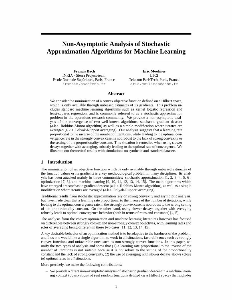
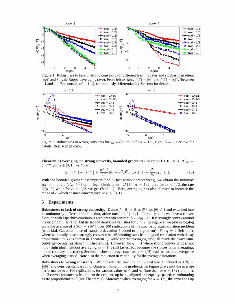
Figure 1: Robustness to lack of strong convexity for different learning rates and stochastic gradient(sgd) and Polyak-Ruppert averaging (ave). From left to right: f(θ) = |θ|2 andf(θ) = |θ|4, (between−1 and1, affine outside of[−1, 1], continuously differentiable). See text for details.

0 2 4−5

0

5

log(n)

log[

f(θ n)−

f∗ ]

α = 1/2

sgd − C=1/5ave − C=1/5sgd − C=1ave − C=1sgd − C=5ave − C=5

0 2 4−5

0

5

log(n)

log[

f(θ n)−

f∗ ]

α = 1

sgd − C=1/5ave − C=1/5sgd − C=1ave − C=1sgd − C=5ave − C=5

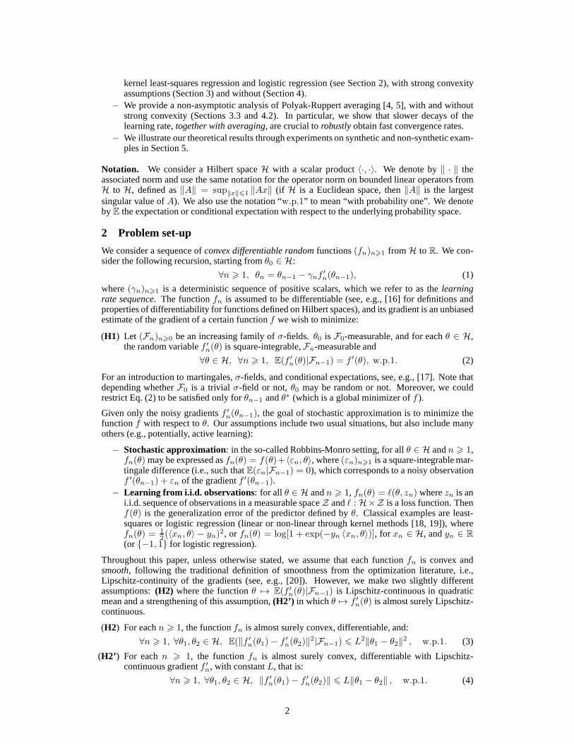
Figure 2: Robustness to wrong constants forγn = Cn−α. Left: α = 1/2, right: α = 1. See text fordetails. Best seen in color.

Theorem 7 (averaging, no strong convexity, bounded gradients) Assume(H1,H5,H8). If γn =Cn−α, for α ∈ [0, 1], we have

E[

f(θn)− f(θ∗)]

6nα−1

2C(δ0 + C2B2ϕ1−2α(n)) +

B2

2nϕ1−α(n). (13)

With the bounded gradient assumption (and in fact without smoothness), we obtain the minimaxasymptotic rateO(n−1/2) up to logarithmic terms [25] forα = 1/2, and, forα < 1/2, the rateO(n−α) while for α > 1/2, we getO(nα−1). Here, averaging has also allowed to increase therange ofα which ensures convergence, toα ∈ (0, 1).

5 Experiments

Robustness to lack of strong convexity. Definef : R → R as|θ|q for |θ| 6 1 and extended intoa continuously differentiable function, affine outside of[−1, 1]. For all q > 1, we have a convexfunction with Lipschitz-continuous gradient with constantL = q(q−1). It is strongly convex aroundthe origin forq ∈ (1, 2], but its second derivative vanishes forq > 2. In Figure 1, we plot in log-logscale the average off(θn) − f(θ∗) over 100 replications of the stochastic approximation problem(with i.i.d. Gaussian noise of standard deviation 4 added tothe gradient). Forq = 2 (left plot),where we locally have a strongly convex case, all learning rates lead to good estimation with decayproportional toα (as shown in Theorem 1), while for the averaging case, all reach the exact sameconvergence rate (as shown in Theorem 3). However, forq = 4 where strong convexity does nothold (right plot), without averaging,α = 1 is still fastest but becomes the slowest after averaging;on the contrary, illustrating Section 4, slower decays (such asα = 1/2) leads to faster convergencewhen averaging is used. Note also the reduction in variability for the averaged iterations.

Robustness to wrong constants. We consider the function on the real linef , defined asf(θ) =12 |θ|2 and consider standard i.i.d. Gaussian noise on the gradients. In Figure 2, we plot the averageperformance over 100 replications, for various values ofC andα. Note that forα = 1/2 (left plot),the 3 curves for stochastic gradient descent end up being aligned and equally spaced, corroboratinga rate proportional toC (see Theorem 1). Moreover, when averaging forα = 1/2, the error ends up

7

0 1 2 3 4 5

−2.5

−2

−1.5

−1

−0.5

log(n)

log[

f(θ n)−

f∗ ]

Selecting rate after n/10 iterations

1/3 − sgd1/3 − ave1/2 − sgd1/2 − ave2/3 − sgd2/3 − ave1 − sgd1 − ave

0 1 2 3 4

−1.5

−1

−0.5

0

log(n)

log[

f(θ n)−

f∗ ]

Selecting rate after n/10 iterations

1/3 − sgd1/3 − ave1/2 − sgd1/2 − ave2/3 − sgd2/3 − ave1 − sgd1 − ave

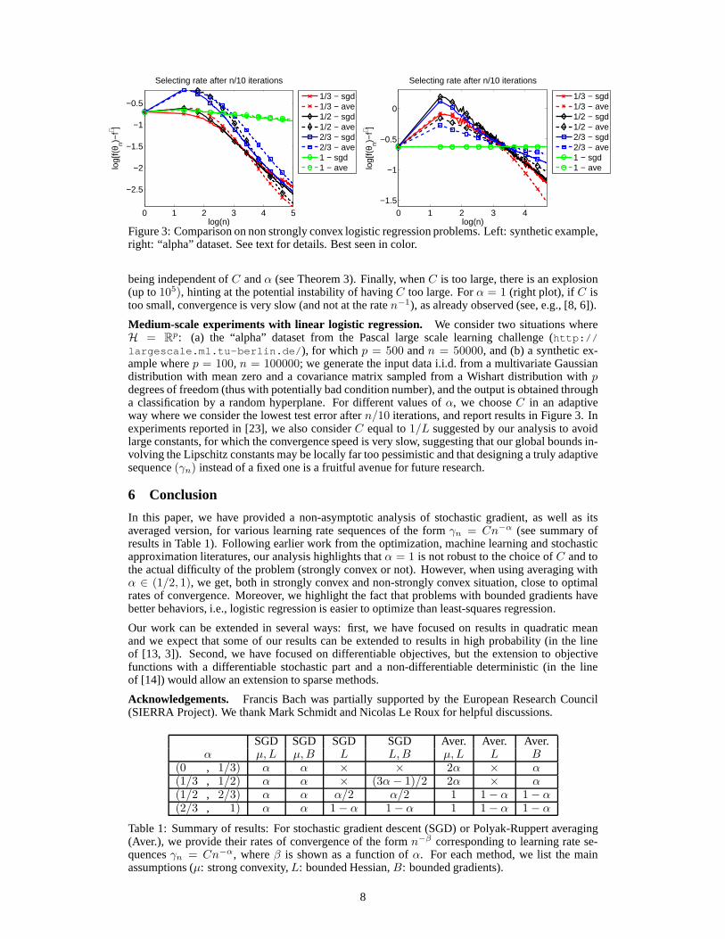
Figure 3: Comparison on non strongly convex logistic regression problems. Left: synthetic example,right: “alpha” dataset. See text for details. Best seen in color.

being independent ofC andα (see Theorem 3). Finally, whenC is too large, there is an explosion(up to105), hinting at the potential instability of havingC too large. Forα = 1 (right plot), if C istoo small, convergence is very slow (and not at the raten−1), as already observed (see, e.g., [8, 6]).

Medium-scale experiments with linear logistic regression. We consider two situations whereH = R

p: (a) the “alpha” dataset from the Pascal large scale learning challenge (http://largescale.ml.tu-berlin.de/), for which p = 500 andn = 50000, and (b) a synthetic ex-ample wherep = 100, n = 100000; we generate the input data i.i.d. from a multivariate Gaussiandistribution with mean zero and a covariance matrix sampledfrom a Wishart distribution withpdegrees of freedom (thus with potentially bad condition number), and the output is obtained througha classification by a random hyperplane. For different values of α, we chooseC in an adaptiveway where we consider the lowest test error aftern/10 iterations, and report results in Figure 3. Inexperiments reported in [23], we also considerC equal to1/L suggested by our analysis to avoidlarge constants, for which the convergence speed is very slow, suggesting that our global bounds in-volving the Lipschitz constants may be locally far too pessimistic and that designing a truly adaptivesequence(γn) instead of a fixed one is a fruitful avenue for future research.

6 Conclusion

In this paper, we have provided a non-asymptotic analysis ofstochastic gradient, as well as itsaveraged version, for various learning rate sequences of the form γn = Cn−α (see summary ofresults in Table 1). Following earlier work from the optimization, machine learning and stochasticapproximation literatures, our analysis highlights thatα = 1 is not robust to the choice ofC and tothe actual difficulty of the problem (strongly convex or not). However, when using averaging withα ∈ (1/2, 1), we get, both in strongly convex and non-strongly convex situation, close to optimalrates of convergence. Moreover, we highlight the fact that problems with bounded gradients havebetter behaviors, i.e., logistic regression is easier to optimize than least-squares regression.

Our work can be extended in several ways: first, we have focused on results in quadratic meanand we expect that some of our results can be extended to results in high probability (in the lineof [13, 3]). Second, we have focused on differentiable objectives, but the extension to objectivefunctions with a differentiable stochastic part and a non-differentiable deterministic (in the lineof [14]) would allow an extension to sparse methods.

Acknowledgements. Francis Bach was partially supported by the European Research Council(SIERRA Project). We thank Mark Schmidt and Nicolas Le Roux for helpful discussions.

SGD SGD SGD SGD Aver. Aver. Aver.α µ,L µ,B L L,B µ, L L B

(0 , 1/3) α α × × 2α × α(1/3 , 1/2) α α × (3α− 1)/2 2α × α(1/2 , 2/3) α α α/2 α/2 1 1− α 1− α(2/3 , 1) α α 1− α 1− α 1 1− α 1− α

Table 1: Summary of results: For stochastic gradient descent (SGD) or Polyak-Ruppert averaging(Aver.), we provide their rates of convergence of the formn−β corresponding to learning rate se-quencesγn = Cn−α, whereβ is shown as a function ofα. For each method, we list the mainassumptions (µ: strong convexity,L: bounded Hessian,B: bounded gradients).

8

References[1] M. N. Broadie, D. M. Cicek, and A. Zeevi. General bounds and finite-time improvement for

stochastic approximation algorithms. Technical report, Columbia University, 2009.[2] H. J. Kushner and G. G. Yin.Stochastic approximation and recursive algorithms and applica-

tions. Springer-Verlag, second edition, 2003.

[3] O. Yu. Kul′chitskiı and A.E. Mozgovoı. An estimate for the rate of convergence of recurrentrobust identification algorithms.Kibernet. i Vychisl. Tekhn., 89:36–39, 1991.

[4] B. T. Polyak and A. B. Juditsky. Acceleration of stochastic approximation by averaging.SIAMJournal on Control and Optimization, 30(4):838–855, 1992.

[5] D. Ruppert. Efficient estimations from a slowly convergent Robbins-Monro process. TechnicalReport 781, Cornell University Operations Research and Industrial Engineering, 1988.

[6] V. Fabian. On asymptotic normality in stochastic approximation.The Annals of MathematicalStatistics, 39(4):1327–1332, 1968.

[7] Y. Nesterov and J. P. Vial. Confidence level solutions forstochastic programming.Automatica,44(6):1559–1568, 2008.

[8] A. Nemirovski, A. Juditsky, G. Lan, and A. Shapiro. Robust stochastic approximation approachto stochastic programming.SIAM Journal on Optimization, 19(4):1574–1609, 2009.

[9] L. Bottou and Y. Le Cun. On-line learning for very large data sets.Applied Stochastic Modelsin Business and Industry, 21(2):137–151, 2005.

[10] L. Bottou and O. Bousquet. The tradeoffs of large scale learning. InAdvances in NeuralInformation Processing Systems (NIPS), 20, 2008.

[11] S. Shalev-Shwartz and N. Srebro. SVM optimization: inverse dependence on training set size.In Proc. ICML, 2008.

[12] S. Shalev-Shwartz, Y. Singer, and N. Srebro. Pegasos: Primal estimated sub-gradient solverfor svm. InProc. ICML, 2007.

[13] S. Shalev-Shwartz, O. Shamir, N. Srebro, and K. Sridharan. Stochastic convex optimization.In Conference on Learning Theory (COLT), 2009.

[14] L. Xiao. Dual averaging methods for regularized stochastic learning and online optimization.Journal of Machine Learning Research, 9:2543–2596, 2010.

[15] J. Duchi and Y. Singer. Efficient online and batch learning using forward backward splitting.Journal of Machine Learning Research, 10:2899–2934, 2009.

[16] J. M. Borwein and A. S. Lewis.Convex Analysis and Nonlinear Optimization: Theory andExamples. Springer, 2006.

[17] R. Durrett.Probability: theory and examples. Duxbury Press, third edition, 2004.[18] B. Scholkopf and A. J. Smola.Learning with Kernels. MIT Press, 2001.[19] J. Shawe-Taylor and N. Cristianini.Kernel Methods for Pattern Analysis. Cambridge Univer-

sity Press, 2004.[20] Y. Nesterov.Introductory lectures on convex optimization: a basic course. Kluwer Academic

Publishers, 2004.[21] K. Sridharan, N. Srebro, and S. Shalev-Shwartz. Fast rates for regularized objectives.Advances

in Neural Information Processing Systems, 22, 2008.[22] N. N. Vakhania, V. I. Tarieladze, and S. A. Chobanyan.Probability distributions on Banach

spaces. Reidel, 1987.[23] F. Bach and E. Moulines. Non-asymptotic analysis of stochastic approximation algorithms for

machine learning. Technical Report 00608041, HAL, 2011.[24] A.S. Nemirovsky and D.B. Yudin.Problem complexity and method efficiency in optimization.

Wiley & Sons, 1983.[25] A. Agarwal, P. L. Bartlett, P. Ravikumar, and M. J. Wainwright. Information-theoretic lower

bounds on the oracle complexity of convex optimization, 2010. Tech. report, Arxiv 1009.0571.[26] E. Hazan and S. Kale. Beyond the regret minimization barrier: an optimal algorithm for

stochastic strongly-convex optimization. InProc. COLT, 2001.[27] G. Casella and R. L. Berger.Statistical Inference. Duxbury Press, 2001.[28] I. Steinwart. On the influence of the kernel on the consistency of support vector machines.

Journal of Machine Learning Research, 2:67–93, 2002.

9