CHAPTER 7

NON-LINEAR.STATIC ANALYSIS OF LAMINATED PLATES

7.1 GENERAL

In the linear analysis of structures, it is assumed that both the displacements and strains

developed in the structure are small. In other words, the geometry of the elements

remains basically unchanged during the loading process and first-order, infinitesimal,

linear strain approximation can be used. In practice, such assumptions fail frequently

eventhough actual strains may be small and elastic limits of ordinary structural materials

not exceeded. In many cases, very large displacements may occur without causing large

strains. If accurate determination of the displacements is needed, geometric non-linearity

may have to be considered in the analysis. When the displacements are large, lateral

deflections are accompanied by stretching of the middle surface, provided that the edges

or at least the comers of the plate are restrained against in-plane motion. Membrane

forces produced by such stretching can help appreciably in carrying the lateral loads.

Small deflection theory is considered to be sufficiently accurate for the analysis of

homogeneous plates if the maximum deflection is less than about half the thickness of the

plate. When the deflection is larger, membrane action also becomes significant, and the

use of a more exact plate theory, which accounts for the geometric non-linearity, has to

be used for the analysis·. It has been reported by Gorji [125] that the small deflection

theory, which is applicable to isotropic plates till about w/h = 0.4, can be valid for

composite laminates only if w/h is much lower. Hence, the analysis of composite

laminates based on large deformation theory is very important.

187

It is observed that the results available in literature are limited to some analytical

solutions and studies based on first-order shear deformation theory. The objective of the

study reported in this chapter is to investigate the effects of geometric non-linearity on

load-deflection behaviour and stress distribution in composite laminates using a finite

element model based on higher-order shear deformation theory accounting for the Von-

Karman non-linear strains. The same 4-noded element with seven degrees of freedom per

node, which was used for the linear analysis, is used in this study also.

7.2 LARGE DEFORMATION THEORY

In large deflection analysis, simultaneous bending and membrane actions resist the lateral

load .. This theory, which is based on Von-Karman's non-linear differential equation,

yields good results for small strains and moderately large deflections and rotations.

For the case of a Mindlin plate, the non-linear Green's strain vector is given as

ex

cy

Y xy ==

y xz

y yz

: + �[(:)' +(:)' +(:)'] : +�[(:)' +(:)' +(:)'] ( au + av ) + au au + av av + aw aw

oy ox ox oy ax ay ax ay

( ou aw ) ou au av av aw aw

az + ox· +oxaz +axaz + ax az

( av aw ) au au av av aw awaz + oy + oy az + ay az + ay az

188

(7.1)

Introducing the Von-Kannan assumptions, which imply that derivatives of u and v withrespect to x, y and z are small, and noting that w is independent of z, allows Green'sstrain to be rewritten as

au +tw)' ou

M:)' ax 2 ox

ax Ex av

+-1{8w

r av

M:)' -oy 2 oy oy Ey (au+ov )

+awaw ou av Yxy

= = -+- + owow (7.2) ay ox ox oy oy --Yxz

ou 8w ax ay (au+aw ) -+- 0 Yyz az ox oz ax

(: +:J av 8w -+-

oz oy 0

Toe higher-order and the product terms in the strain vector represent th� non-linearcomponents of in�plane strain and are expressed as

M:)' ax 8w

H:J' 1 ow ax

(7.3) = - 0 -

2 oy ow -

owaw ow ow oy --

-

ox ay oy ox J

Thus, the generalized Green's strain vector of Eq. (7.2) is expressed as

(7.4)

189

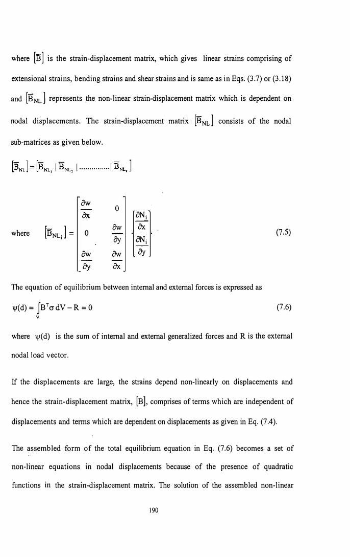
where [B] is the strain-displacement matrix, which gives linear strains comprising of

extensional strains, bending strains and shear strains and is same as in Eqs. (3 :7) or (3 .18)

and [BNL] represents _the non-linear strain-displacement matrix which is dependent on

nodal displacements. The strain-displacement matrix [BNL] consists of the nodal

sub-matrices as given below.

ow 0 aN·

I

[BNLi ] =

ow ox (7.5) where 0

ay aN· I

ow ow ay

ox

The equation of equilibrium between internal and external forces is expressed as

\j/(d) = fBTcrdV-R = 0 (7.6)

where \j/( d) is the sum of internal and external generalized forces and R is the external

nodal load vector.

If the displacements are large, the strains depend non-linearly on displacements and

hence the strain-displacement matrix, [B], comprises of terms which are independent of

displacements and terms which are dependent on displacements as given in Eq. (7.4).

The assembled form of the total equilibrium equation in Eq. (7.6) becomes a set of

non-linear equations in nodal displacements because of the presence of quadratic

functions in the strain-displacement matrix. The solution of the assembled non-linear

190

equilibrium equations gives the nodal displacements, using which the internal stresses are

evaluated.

7.3 FINITE ELEMENT FORMULATION

Finite element formulation for the solution of non-linear problem explained in the

previous section is given below, using a 4-noded element based on HSDT.

The development of [B] matrix in Eq. (7.4) remains the same as that in linear analysis

and is given by Eq. (3.18). [i3NLJ matrix as given in Eq. (7.5) is developed as follows.

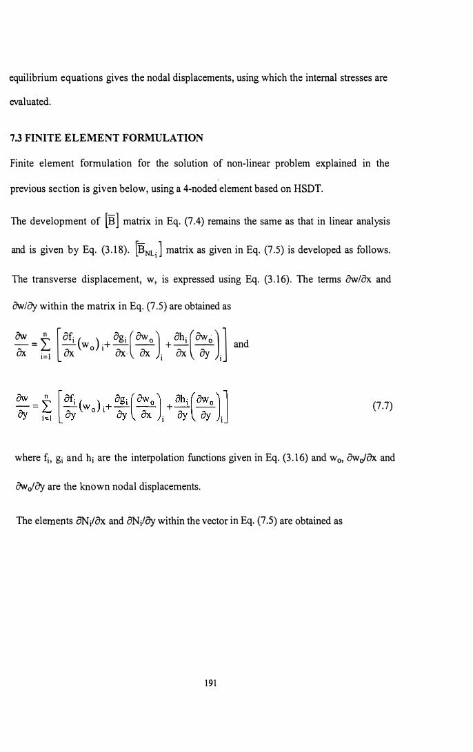
The transverse displacement, w, is expressed using Eq. (3.16). The terms ow/ox. and

owloy within the matrix in Eq. (7.5) are obtained as

ow_ f [afi ( ) 8gi (owo) 8hi (owoJ J d--� -w +--- +--- an

OX i=l OX. O I

OX.· OX. i OX. O'j i

(7.7)

where fi, gi and hi are the interpolation functions given in Eq. (3.16) and w0, owJox. and

owJoy are the known nodal displacements.

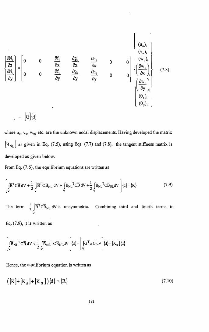
The elements 8N/8x and 8Nj/8y within the vector in Eq. (7.5) are obtained as

191

(uo)i

(vo) i

aNi 0 0 ari 8gi Bhi 0 0 (wo)i

ax ax ax

(8:o

J = (7.8)

aNj ari agi 8hi 0 0 0 0

ay oy oy ay

(�'J (0x )i

(0y) i

= [G]{ct}

where Uo, Vo, Wo, etc. are the unknown nodal displacements. Having developed the matrix

[BNL] as given in Eq. (7.5), using Eqs. (7.7) and (7.8), the tangent stiffness matrix is

developed as given below.

From Eq. (7.6), the equilibrium equations are written as

[ JET CB dV + _!_ .fBT CBNL dV + .fBNL T CB dV + ..!.. JBNL

T CBNL dV l {d} = {R}v

2v v

2v

(7.9)

The term 1 JB1 CBNL dV is unsymmetric. Combining third and fourth terms m

Eq. (7.9), it is written as

Hence, the equilibrium equation is written as

( [K]+ [KJ+ [K0 ]){d} = {R} (7.10)

192

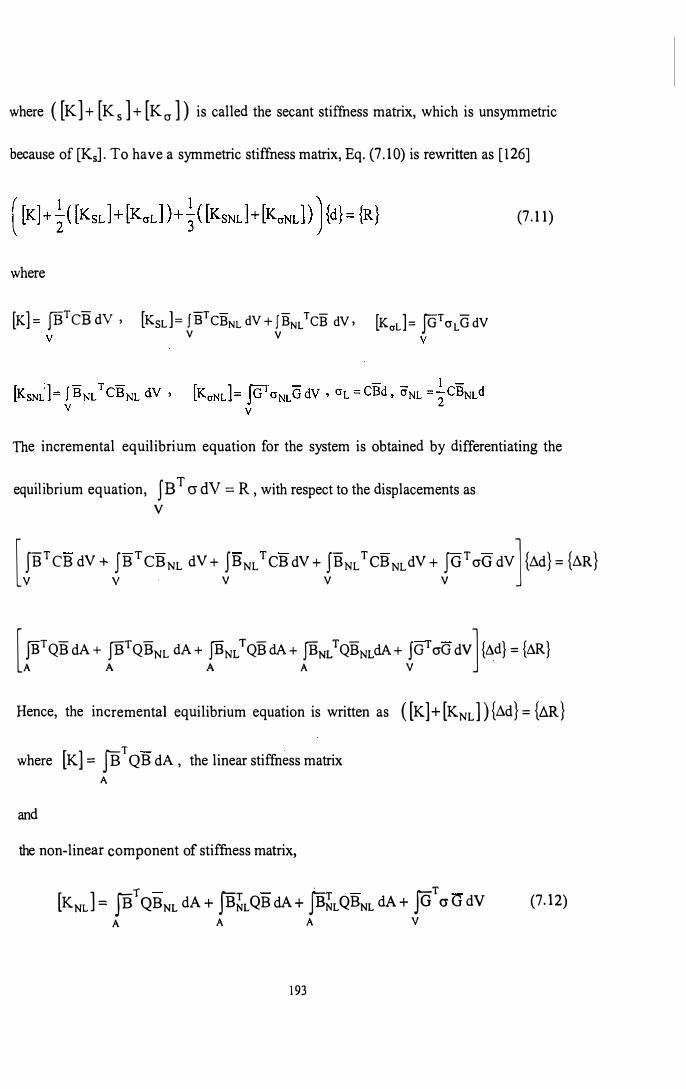
where ( [K ]+[Ks]+ [K cr ]) is called the secant stiffness matrix, which is unsymmetric because of [K 5]. To have a symmetric stiffness matrix, Eq. (7.10) is rewritten as [126]

where [K]= fiFCBdV, [Ksd= fiFcBNL dV + JBNLrcB dV,

V V

(7.11)

[K0d= J<FcrLG dV

The incremental equilibrium equation for the system is obtained by differentiating the equilibrium equation, f BT cr dV = R, with respect to the displacements as

V

[ fBr CB dV + f B T CBNL dV + fBNL r CB dV + fBNL r CBNLdV + f G r aG dv] {fld} = {flR} V V · V V V

[jlFQB dA+ fBTQBNL dA+ JBNLTQBdA+ JBN/QBNLdA+ JGTaG dv]{fld} = {flR} A A A A V

Hence, the incremental equilibrium equation is written as ([K]+[K NL]){fld}= {AA} where [ K] = jB T QB dA ' the linear stiffness matrix

A

and the non-linear component of stiffness matrix,

[K NJ = jB r QBNL dA + JB�L QB dA + jB�L QBNL dA + Jct a G dV (7 .12) A A A V

193

7.4 SOLUTION PROCEDURES

Basically, there are two. distinct approaches for the solution of non-linear equations of

equilibrium: (i) direct solution of the non-linear equations by iterative procedure and

(ii) piece-wise linear load incrementing method. In either of these numerical methods, it

is assumed that during each solution cycle, the stiffness analysis proceeds along a

straight-line tangent to the curve characterising the force-deflection relations of the

structure. In order to achieve such a tangent solution, the stiffness matrix of each element

should be modified to account for the accumulated stresses and the change in geometry.

7.4.1 Direct Method

For a given set of external loads, the objective of non-linear analysis is to determine the

true values of displacements and internal stresses. Since the tangent stiffness matrix is

dependent on the instantaneous strains and displacements, an iterative method of solution

is inevitable. Newton-Raphson method of successive cycles of linear analysis has been

used in the solution of a variety of non-linear structural analysis problems with extremely

satisfactory performance. The basic principles of this method are outlined below.

Using the initial geometry and the external loads, a linear stiffness analysis is performed

first. Result of this analysis is used as a trial solution for the iterative procedure. Using

this trial solution, the non-linear part of the stiffness matrix, given in Eq. (7.12), is

evaluated. At a particular node of the system, in the direction of a particular degree of

freedom, the algebraic sum of all the calculated stress resultants must be equal to the

external load applied in that particular direction. Since, the nodal displacements obtained

in the first cycle do not correspond to the true equilibrium geometry, the algebraic sum of

the internal stress resultants obtained using this first set of approximate displacements

194

will not be equal to the given external loads. The difference between the internal and

external forces constitutes the unbalanced nodal loads to be used in the next cycle of

analysis. Using the tangent stiffness matrix evaluated including the non-linear

components and the unbalanced nodal forces, a set of nodal displacements is calculated.

This gives a correction to be applied to the trial solution. When the nodal displacements

of the first and the second cycles are superimposed, the system comes closer to the actual

equilibrium configuration. As a result, the difference between the external loads and the

stress resultants, calculated on the basis of the corrected nodal displacements, is reduced.

Using the new unbalanced nodal forces and new stiffness matrix based on the corrected

nodal displacements, a new set of corrections to displacements is obtained which is

superimposed with the nodal displacements obtained in the previous cycle. A new set of

unbalanced nodal forces is calculated based on the new set of displacements. The above

iterative process is repeated until the maximum unbalanced nodal force in any direction

becomes less than a tolerable value. The tangent stiffness matrices are modified after

each cycle to include the latest strains and displacements.

The above procedure can be employed in two ways. Either the total load can be applied

in a single step or the total load can be applied in increments by dividing the total load

into a number of load steps, in which case iterations are required at each of the load steps.

The latter method improves numerical stability and gives intermediate results enabling

the understanding of load-deflection behaviour characteristics. In order to reduce the

computational effort involved in the latter method, a modified version of the above

procedure has been developed, referred to as modified Newton-Raphson method. In this

method, the tangent stiffness matrix is evaluated once only on the second iteration of

195

each load increment. In this method, relatively large load increments are generally

suitable. Behaviour predictions are independent of increment size, since solutions are

obtained to the actual non-linear model.

7.4.2 Piece-wise Linear Load Incrementing Method

Selection of linear load incrementing method exchanges the problem of solving the

multidimensional, non-linear equations for a multiplicity of linear solutions. This method

is recommended by its linearisation. The solution of sets of linear equations is readily

accomplished. The procedure involved in this method is outlined below.

The total load on the system is divided into a number of load steps and the starting

solution is obtained by performing a linear stiffness analysis for the first load step. The

displacements obtained from this step will be used to evaluate the non-linear components

of stiffness matrix. This matrix along with the linear part of stiffness matrix is used to

evaluate displacements for the next load step. These displacements are added to the

displacements for the first load step. These net displacements will be used for the

evaluation of stiffness matrix in the next load step. This process is continued until the last

load step is completed. Thus, in this method, no iteration at constant load is required,

which, in tum, means that there is no danger of a divergence of the solution. Control is

exercised over the accuracy of the incremental analysis by control of the increment size

which, in tum, depends upon load-displacement behaviour. As a consequence, the

apparent speed advantage of an incremental method can be expended in multiple

executions designed to improve or build confidence in the predicted behaviour. An

undersized increment will be wasteful, since it results in an excessive number of linear

solutions.

196

7.5 NUMERICAL RESULTS

Studies based on higher-order shear deformation theory are conducted to investigate the

effects of geometric non-linearity on load-deflection behaviour and stresses of composite

laminates.

7.5.1 Validation

The validation of the program is done by considering few examples for which results are

available in literature. Reduced integration scheme is used for the evaluation of both

bending and transverse shear terms of stiffness matrix and a mesh division of 16x 16 for

full plate is used for the analysis.

Example 7.1

Square isotropic plates of width-to-thickness ratios 10 and 100, with all the edges

clamped and subjected to a uniform load of non-dimensional value, Q = 200 and 402

respectively, for which results have been given by Shukla and Nath [63] and Pica

et aL [127], are considered first. As the method of linear piece-wise incremental

procedure necessitates smaller load steps, the load, Q, has been incremented in steps of 1.

But for the Newton-Raphson iterative procedure, the load, Q, has been incremented in

steps of 4 and a relative convergence criteria of 0.01 % at every step of loading has been

employed. The results obtained by adopting Newton-Raphson iterative technique and

piece-wise linear incremental technique for the thick plate are presented in Table 7.1 in

non-dimensional form as w = w I h and are compared with available results. Agreement

in results is found to be very good. The load-deflection variation for the thick and thin

plates is presented in Figs. 7 .1 and 7 .2 along with the corresponding linear solution.

197

·t;;Load, Q

�i \'

20

40

80

120

200

Table 7 .1 Comparison of non-dimensional central deflection for clamped isotropic plate, b/h = 10 ( v = 0.3)

w

Present analysis

Shukla and Linear load

N ewton-Raphson incrementing

Nath [63] method

method

0.3074 0.3101 0.3096

0.5441 0.5535 0.5525

0.8649 0.8849 0.8848

1.0852 1.1109 1.1128

1.3958 1.4271 1.4336

198

Turvey and Osman [128]

0.3017

0.5423

0.8655

1.0860

1.3980

3.5

... Newton-Raphson method

3.0 * Linear load incrementing method

Linear

2.5

2.0

I�

1.5

1.0

0.5

0.0

0 40 80 120 160 200

Load, Q

Figure 7 .1 Load-deflection behaviour of clamped isotropic plate (b/h = 1 O)

6.0 ,------------------,

5.0

4.0

I� 3.0

2.0

1.0

* Newton-Raphson method

Linear load incrementing metho

Linear

Exact [129)

0.0 .... ---r--�----,---.---r----j

0 80 160 240

Load, Q

320 400 480

Figure 7 .2 Load-deflection behaviour of clamped isotropic plate (b/h = 100)

199

From Table 7 .1 and Figs. 7 .1 and 7 .2, it is seen that the results predicted using a large

load step by Newton-Raphson iteration and a small load step by piece-wise incremental

procedure are almost the same. But, the latter method requires less computational effort

and also the first method exhibited some computational instability in some cases for

higher loads. Hence, the piece-wise linear incremental procedure has been employed for

further studies.

The exact central normal stress expressed in non-dimensional form, ax

= crxb2 / Eh2 for

the thin plate corresponding to the total load, Q == 402, has been reported to be 25.1 [129].

The present study gives a value of 24.66, showing good agreement.

Example 7.2

To validate the program for composite laminates, a clamped 2-layer cross-ply (0/90)

laminate given by Shukla and Nath [63] and a simply supported 2-layer angle-ply

(45/-45) laminate given by Barbero and Reddy [58] are considered. The geometry and the

material properties of the J?lates are as given below.

Cross-ply: a = b = lm, h = O.lm, E1 = 175.78 GPa , E1/E2 = 25, Gn/E2 = G13/E2 = 0.5, G23/E2 = 0.5, V12

= 0.25.

Angle-ply: a = b = lm, h = 0.002m, E1 = 250 GPa, E2 = 20 GPa, G12 = G13 = 10 GPa, G23 = 4 GPa, v12

= 0.25.

The boundary conditions used are as follows:

at x = 0 and x = a, at y = 0 and y = b,

Vo = w O = aw of oy = Sy = 0 Uo = Wo = awof8x = 9x = 0

The non-dimensional central deflections obtained are presented in Figs. 7 .3 and 7.4. In

both cases, results of the present analysis agree very well with available results.

200

' •. _·:f:

2.0 ,---------------.,Present analysis

* Linear

1.5

I� 1.0

0.5

•

+

Shukla and Nath [63]

Singh et al. [130]

0.0 --------.-----,.------'--r-----.---�

0 · 60 120 180 240 300

Load, Q

Figure 7 .3 Load-deflection behaviour of 2-layer cross-ply (0/90) laminate

4.0 -.-------------------,

3.0

I� 2.0

1.0

Present analysis

* Linear

• Barbero and Reddy [58)

0.0 �----ir----,---,-----.---;

0 15 30 45 60 75

Load, Q

Figure 7.4 Load-deflection behaviour of 2-layer angle-ply (45/-45) laminate

201

7.5.2 Parametric Study

To study the effect of various parameters on the non-linear behaviour of composite

plates, numerical studies are carried out by analyzing plates having the following

geometric and material properties.

a = b = 1.0 m, E 1 = 175.0GPa, E2 = 7.0GPa, v12 = 0.25, G12 = G13 = 3.SGPa,

G23 = l.4GPa

In all cases, a uniform load of non-dimensional value, Q = 300 is applied in steps of 1,

unless otherwise specified.

Effect of width-to-thickness ratio (b/h)

Example 7.3

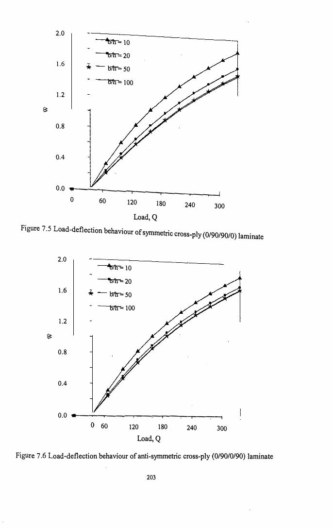
To study the effect of width-to-thickness ratio on the non-linear behaviour, 4-layer

cross-ply (0/90/90/0 and 0/90/0/90) and angle-ply (45/-45/-45/45 and 45/-45/45/-45)

laminates are considered. The non-dimensional values of central deflection for symmetric

and anti-symmetric cross-ply laminates with the edges simply supported are plotted in

Figs. 7 .5 and 7 .6 respectively. From these figures, it is evident that the non-dimensional

deflection decreases with increase in b/h ratio and the behaviour of plates with width-to­

thickness ratio beyond 50 is almost the same. The variation of stresses through the

thickness of thick and thin symmetric cross-ply laminates, non-dimensionalised as in

Eq. (3.14), is shown in Figs. 7.7 and 7.8, along with the linear solutions.

202

- -

2.0 bib= 10

bib =20 1.6

* bib= 50

bib== 100

1.2

I�

0.8

0.4

0.0 .----,----,-----.----.----10 60 120 180 240 300

Load,Q

Figure 7.5 Load-deflection behaviour of symmetric cross-ply (0/90/90/0) laminate

I:!=

2.0 bib= 10

bib =20

1.6 * bib= 50

bib= 100

1.2

0.8

0.4

0.0 ------..-----,r-----r----.-----i

60 120 180

Load, Q

240 300

Figure 7 .6 Load-deflection behaviour of anti-symmetric cross-ply (0/90/0/90) laminate

203

0.4746 0.0556 0.0238

I

I

0.8153 0.3919

O'x 'ixy

0-0,

0.0604

--Linear

---- Non-linear

0.4155

Tyz

V•-'YDo 0.9405

) 0)2716 0.5016

/ /,,.

Txz

Figure 7. 7 Stress variation across the thickness of symmetric cross-ply laminate (b/h = 10)

N 0 V.

I

0.8296 0.5679

crx

0.6303 0.0394 0.0232 �-��

\

\

Txy

0.0423

--Linear

---- Non-linear

4.0874 0.2544 \ \ f 0.1165 / 0.3392 I

n I

Tyz

--· . x- , 1.0280 I l

.4136 0.5483

Txz

Figure 7 .8 Stress variation across the thickness of symmetric cross-ply laminate (b/h = 100)

The non-dimensional values of central deflection for symmetric and anti-symmetric

angle-ply laminates with the edges simply supported are given in Figs. 7 .9 and 7 .10. The

behaviour is same as that of simply supported cross-ply laminates. Anti-symmetric

angle-ply laminates have lower values of deflection than for symmetric laminates, as is

seen from the figures.

1.2

1.0

0.8

I� 0.6

0.4

0.2

b/h= 10

b/h =20

b/h= 50

b/h = 100

0.0 4-----r---.----.-----.---1

0 60 120 180 240 300

Load, Q

Figure 7.9 Load-deflection behaviour of symmetric angle-ply (45/-45/-45/45) laminate

206

1.0

b/h = 10

* b/h=20

0.8 b/h = 50

b/h = 100

0.6

I�

0.4

0.2

0.0

0 60 120 180 240 300

Load, Q

Figure 7 .10 Load-deflection behaviour of anti-symmetric angle-ply ( 45/-45/45/-45) laminate

The non-dimensional values of central deflection for symmetric cross-ply (0/90/90/0)

laminates of different width-to-thickness ratios and the edges clamped are plotted in

Fig. 7 .11. It is seen that there is a decrease in deflection of around 5% from b/h = 50 to

100, whereas the load-deflection curve is almost the same for b/h = 50 and 100 in the

case of simply supported edge conditions.

207

� . .

1.0

0.8

0.6

I�

0.4

0.2

0.0

0

• b/h= 10

b/h=20

* b/h= 50

60 120 180

Load, Q

240 300

Figure 7.11 Load-deflection behaviour of clamped cross-ply (0/90/90/0) laminate

The effect of b/h ratio on the load-deflection behaviour of simply supported and clamped

symmetric cross-ply laminates corresponding to a maximum load, Q = 300 is depicted in

Fig. 7 .12. Even though the variation of linear solution is different in thick plate region for

the two edge conditions, the non-linear solution follows the same variation irrespective of

edge conditions.

208

I�

4.0

3.5

3.0

2.5

2.0

1.5

1.0 *·-

0.5

0

.t. Linear (Simply supported)

- - -.a.- - - Nonlinear (Simply supported)

* Linear (Clamped)

- - -•- - - Nonlinear (Clamped)

.... ______ _ ---"* · -------------------

20 40 60 80 100

b/h

Figure 7 .12 Comparison of linear and non-linear deflections

. .

A comparison of degree of non-linearity for simply supported symmetric cross-ply and

angle-ply laminates is given in Fig. 7 .13. From the figure, it is clear that the fibre

orientation angle does not influence the non-linear behaviour of laminates except that the

degree of non-linearity is less for angle-ply laminates. Moreover, the degree of non-

linearity increases with increase in b/h ratio.

Figure 7.14 shows the variation of degree of non-linearity for simply supported and

clamped cross-ply (0/90/90/0) laminates. It is evident that the degree of non-linearity is

less for clamped plates in thick range compared to simply supported plates. For simply

supported plates, degree of non-linearity does not vary much beyond b/h = 20, whereas in

the case of clamped plates, the degree of non-linearity goes on increasing upto b/h = 50.

209

1.0

... 0/90/90/0

i ;. 45/-45/-45/45

C:

�

is 0.8·t::� 11)

;.§ I c::

0

'-0

0.6

0

0.4 -t---.----.----.-----.----J 0 20 40 60 80 100

b/h

Figure 7.13 Variation of degree of non-linearity with b/h ratio

1.0

A Simply supported

* Clamped

t 0.8

;

b 't:: C"a 11) c::

0.6 .... I

c:: 0 c::

I...., 0

11)

11)

0.4 11)

0

0.2

0 20 40 60 80 100

b/h

Figure 7 .14 Degree of non-linearity for cross-ply laminates

210

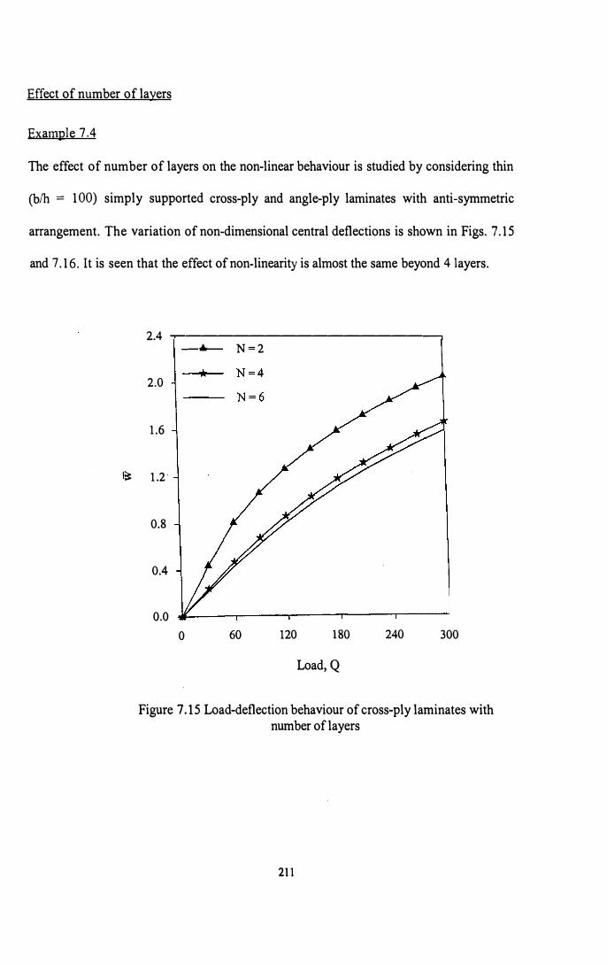
Effect of number of layers

Example 7.4

The effect of number of layers on the non-linear behaviour is studied by considering thin

(b/h = 100) simply supported cross-ply and angle-ply laminates with anti-symmetric

arrangement. The variation of non-dimensional central deflections is shown in Figs. 7 .15

and 7 .16. It is seen that the effect of non-linearity is almost the same beyond 4 layers.

2.4 -,-------------------,

2.0

1.6

I� 1.2

0.8

0.4

0.0

0

.t. N=2

60 120 180 240 300

Load,Q

Figure 7 .15 Load-deflection behaviour of cross-ply laminates with number of layers

211

1.0

0.8

0.6

I�

0.4

0.2

• N=2

0.0 .----.----.------,----..------1

0 60 120 180 240 300

Load, Q

Figure 7 .16 Load-deflection behaviour of angle-ply laminates with number of layers

Effect of in-plane edge conditions

Example 7.5

To study the effect of in-plane edge conditions on the non-linear behaviour, two different

simply supported boundary conditions are considered for the analysis. (i) Plate with

movable edges (SS 1) and (ii) Plate with immovable edges (SS2) as given below.

SS 1: at x = 0 and x = a,

at y = 0 and y = b,

SS2: atx = Oandx= a,

at y = 0 and y = b,

Vo = Wo = EJwJay = 0y = 0

Uo = Wo = EJwJox = 0x = 0

Uo= Vo= Wo = EJwJay= 0y= 0

Uo = Vo= Wo = EJwofox = 0x = 0

212

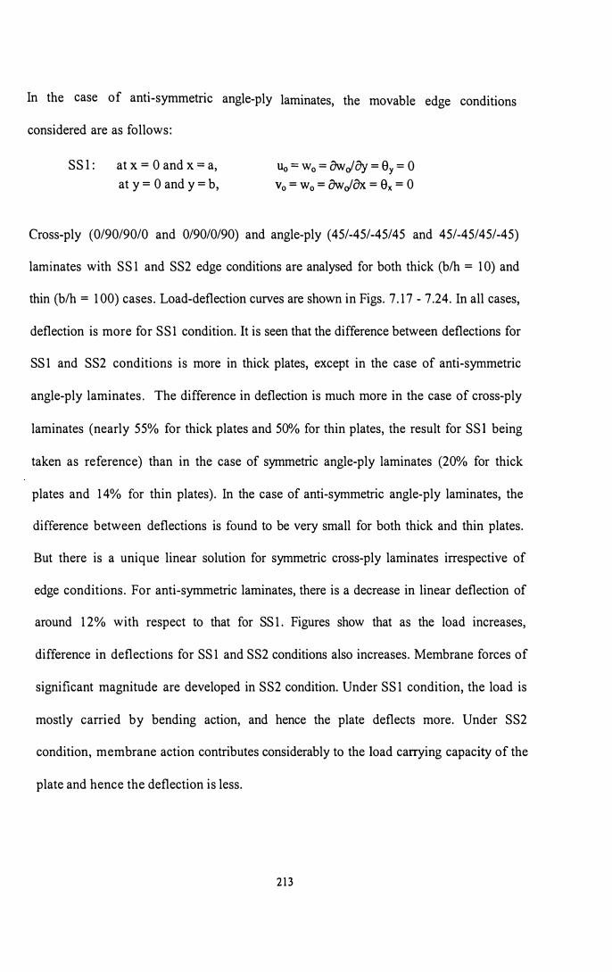
In the case of anti-symmetric angle-ply laminates, the movable edge conditions

considered are as follows:

SSl: at x = 0 and x = a,

at y = 0 and y = b,

Uo= w0

= 8wJoy= Sy

= 0

Vo = Wo = 8wJox = Sx = 0

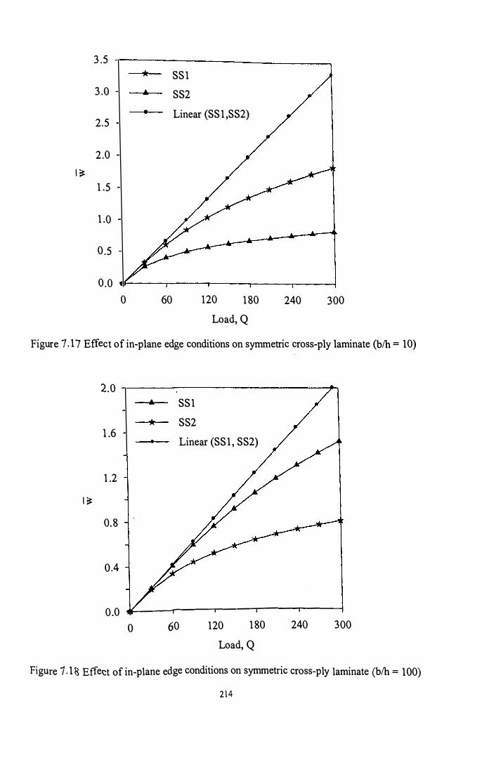
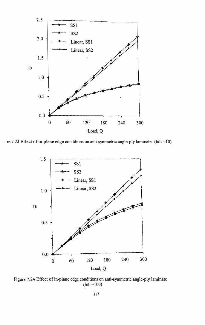
Cross-ply (0/90/90/0 and 0/90/0/90) and angle-ply ( 45/-45/-45/45 and 45/-45/45/-45)

laminates with SS 1 and SS2 edge conditions are analysed for both thick (b/h = 10) and

thin (b/h = 100) cases. Load-deflection curves are shown in Figs. 7.17 - 7 .24. In all cases,

deflection is more for SS 1 condition. It is seen that the difference between deflections for

SS 1 and SS2 conditions is more in thick plates, except in the case of anti-symmetric

angle-ply laminates. The difference in deflection is much more in the case of cross-ply

laminates (nearly 55% for thick plates and 50% for thin plates, the result for SSl being

taken as reference) than in the case of symmetric angle-ply laminates (20% for thick

plates and 14% for thin plates). In the case of anti-symmetric angle-ply laminates, the

difference between deflections is found to be very small for both thick and thin plates.

But there is a unique linear solution for symmetric cross-ply laminates irrespective of

edge conditions. For anti-symmetric laminates, there is a decrease in linear deflection of

around 12% with respect to that for SS 1. Figures show that as the load increases,

difference in deflections for SS 1 and SS2 conditions also increases. Membrane forces of

significant magnitude are developed in SS2 condition. Under SS 1 condition, the load is

mostly carried by bending action, and hence the plate deflects more. Under SS2

condition, membrane action contributes considerably to the load carrying capacity of the

plate and hence the deflection is less.

213

3.5 * SS1

3.0 ... SS2

2.5 Linear (SS1,SS2)

2.0

I�

1.5

1.0

0.5

0.0

0 60 120 180 240 300

Load, Q

Figure 7 .17 Effect of in-plane edge conditions on symmetric cross-ply laminate (b/h = 10)

2.0 ... SS1

* SS21.6

Linear (SS1, SS2)

1.2

I�

0.8

0.4

0.0 J£._---r----r----,----.----1

0 60 120 180 240 300

Load, Q

Figure 1.1 � Effect of in-plane edge conditions on symmetric cross-ply laminate (b/h = 100)

214

3.5

3.0

2.5

2.0

I�

1.5

1.0

0.5

0.0

0

4 SS1

* SS2

Linear, SS1

i Linear, SS2

60 120 180

Load, Q

240 300

Figure 7 .19 Effect of in-plane edge conditions on anti-symmetric cross-ply laminate (b/h =1 O)

2.5

SS1

... SS2 2.0

Linear, SS1

Linear, SS2

1.5

I�

1.0

0.5

0.0 �---..-----r---.----.----i

0 60 120 180 240 300

Load, Q

Figure 7 .20 Effect of in-plane edge conditions on anti-symmetric cross-ply laminate (b/h =l 00)

215

2.5

SS1

... SS2 2.0

Linear (SS l ,SS2)

1.5

I�

1.0

0.5

0.0 ...----,----,----.-----.-----l

0 60 120 180 240 300

Load, Q

Figure 7.21 Effect of in-plane edge conditions on symmetric angle-ply laminate (b/h =10)

I�

1.5

1.0

0.5

... SS1

* SS2

Linear (SS1, SS2)

0.0 ,M.----.-----r----r----,-----j

0 60 120 180 240 300

Load, Q

Figure 7.22 Effect of in-plane edge conditions on symmetric angle-ply laminate (b/h =100)

216

2.5 * SS1

... SS22.0

i Linear, SS1

Linear, SS2

1.5

I�

1.0

0.5

0.0

0 60 120 180 240 300

Load, Q

, re 7.23 Effect of in-plane edge conditions on anti-symmetric angle-ply laminate (b/h =10)

1.5 * SS1

... SS2

+ Linear, SS1

1.0 Linear, SS2

I�

0.5

0.0

0 60 120 180 240 300

Load, Q

Figure 7.24 Effect of in-plane edge conditions on anti-symmetric angle-ply laminate

(b/h =100)

217

Effect of aspect ratio

Example 7.6

The influence of aspect ratio on the central transverse displacement of thin (b/h = 100)

symmetric cross-ply (0/90/90/0) and angle-ply (45/-45/-45/45) laminates with simply

supported boundary conditions is shown in Figs. 7.25 and 7.26. It is seen that the non­

linearity increases as alb increases in the case of both the laminates.

4.0

alb= 1.0

3.5 * alb= 1.5

3.0 alb =2.0

t alb= 2.5

2.5

I� 2.0

1.5

1.0

0.5

0.0

0 60 120 180 240 300

Load,Q

Figure 7 .25 Change in load-deflection behaviour of cross-ply laminates with aspect ratio

218

3.5

alb= 1.0

3.0 * alb= 1.5

alb= 2.0

2.5 alb= 2.5

2.0

•I�

1.5

1.0

0.5

0.0

0 60 120 180 240 300

Load, Q

Figure 7 .26 Change in load-deflection behaviour of angle-ply laminates with aspect ratio

7.6 DISCUSSION

Based on the studies conducted, the following observations are made:

1. Piece-wise linear load incrementing method and Newton-Raphson iterative

procedure give almost the same results. But, the difficulty of divergence of

solution under higher loads by the iterative procedure can be avoided by using

piece-wise linear load incrementing method.

2. Degree of non-linearity is more in cross-ply laminates than m angle-ply

laminates.

219

3. Degree of non-linearity is more in simply supported plates compared to clamped

plates in the thick range whereas the reverse is the case in thin range.

4. Angle of fibre orientation does not have any influence in the non-linear

behaviour pattern of composite plates.

5. The non-linear load deflection behaviour is the same beyond 4 layers.

6. The in-plane edge conditions play an important role in the non-linear behaviour

which is not predominant in the linear analysis.

7. The studies conducted confirm that the small deflection theory is applicable in

the case of composite laminates only if w/h is less than 0.2.

8. The simple finite element model chosen for the study is found to be sufficient for

large displacement analysis oflaminated composite plates.