Nominal Bonds, Real Bonds, and Equity∗

Andrew AngMaxim Ulrich

Columbia University

This Version: April 2012

JEL Classification: G12, E31, E42, E52Keywords: term structure, yield curve, equity risk premium,

Fed model, TIPS, Taylor rule

∗We thank Martin Lettau and Stijn Van Nieuwerburgh for helpful comments.

Nominal Bonds, Real Bonds, and Equity

Abstract

We decompose the term structure of expected equity returns into (1) the real short rate, (2) a

premium for holding real long-term bonds, or the real duration premium, the excess returns of

nominal long-term bonds over real bonds which reflects (3) expected inflation and (4) inflation

risk, and (5) a real cashflow risk premium, which is the excess return of equity over nominal

bonds. All of these risk premiums vary over time. The shape of the unconditional nominal

and real bond yield curves are upward sloping due to increasing duration and inflation risk

premiums. The average term structures of expected equity returns and equity risk premiums, in

contrast, are downward sloping due to the decreasing effect of short-term expected inflation, or

trend inflation, across horizons. Around 70% of the variation of expected equity returns at the

10-year horizon is due to variation in the output gap and trend inflation.

1 Introduction

While recent research has made considerable progress in understanding the term structure of

nominal Treasury yields and real TIPS yields, the term structure of expected equity returns and

their macroeconomic relation to the nominal and real yield curves is less well understood.1

This is surprising because the difference between nominal bond and real yields, or inflation

compensation, is the sum of expected inflation and the inflation risk premium and the equity

price-dividend ratio is the expected present value of future real dividend growth discounted

using risk-adjusted real bond yields. Thus, macroeconomic factors that are known to drive the

nominal and real term structures should potentially also contain information about expected

equity returns and equity risk premiums.

We build a model that prices nominal bonds, real bonds, and equity in a unified framework

and examine their combined term structures. We decompose the term structure of expected

equity returns into (1) the real short rate, (2) a real duration premium for holding long-term real

bonds, (3) expected inflation, (4) the inflation risk premium, where (3) and (4) are reflected in

long-term nominal bonds, and (5) a real cashflow risk premium, which is the expected equity

return in excess of a long-term nominal bond yield.2 Each of these components have their

own term structures. Using the model, we show how variations in economic growth, inflation,

monetary policy, and real dividend growth affects each of these risk premium components over

time and across holding periods.

Pricing equity requires discounting future real cashflows using real interest rates and real

risk premiums. While a complete term structure of nominal bonds is available over long periods,

only long-term real bond prices are observed in data in the most recent sample. Real short rates

and real risk premiums needed to discount future real cashflows are empirically unobserved

1 The modeling of equity and bonds has largely developed separately but has made considerable progress over

the last two decades. For reduced-form bond models with latent and macro factors, see, among many others, Duffie

and Kan (1996), Dai and Singleton (2000, 2002, 2003), and Ang and Piazzesi (2003). Equilibrium bond pricing

models are developed by Cox, Ingersoll and Ross (1985), Buraschi and Jiltsov (2005), Wachter (2006), Piazzesi and

Schneider (2006), Ulrich (2010, 2011a), and Bansal and Shaliastovich (2010), among others. Reduced-form equity

valuation models are derived by Fama and French (1988), Ang and Liu (2001), Ang and Bekaert (2007), Lettau

and Ludvigson (2005), Lettau and Wachter (2007), among others. A large equilibrium equity-pricing literature

includes Mehra and Prescott (1987), Bansal and Yaron (2004), Campbell and Cochrane (1999), Menzly, Santos

and Veronesi (2004), and Lettau, Ludvigson and Wachter (2008), among others.2 Our breakdown is similar to Ibbotson and Chen (2003), but unlike Ibbotson and Chen they are time varying

and consistently derived in one overall model.

1

(see also comments by Lettau and Wachter (2010)). We endogenize the unobserved real pricing

kernel by using the rich available data for nominal and real bonds, realized inflation, together

with a specification for inflation risk premiums.

We first model nominal bonds by building on a large macro-term structure literature. We

follow Taylor (1993) and assume the Federal Reserve (Fed) sets the Fed Funds rate as a func-

tion of the output gap and trend inflation (or short-term expected inflation) as well as monetary

policy shocks. Through no arbitrage, nominal yields are risk-adjusted expectations about future

Fed Funds rates and reflect macro risk premiums. After defining the nominal pricing kernel,

inflation, and inflation risk premiums, the model endogenously generates the real pricing ker-

nel. The real short rate depends on the same macro variables that enter the nominal Taylor

rule but has different loadings which reflect the covariance of inflation shocks with the macro

variables and inflation risk. While the majority of affine term structure models rely on latent

factors extracted from yields to obtain a close fit to data (see, for example, the summary by

Piazzesi (2010)), we are able to price nominal and real bonds with only macro variables – the

output gap, trend inflation, and monetary policy shocks.3

Equity is a bond perpetuity with stochastic real dividend cashflows. We price the real div-

idend stream using the implied real pricing kernel and assume the cashflow shock is priced,

which gives rise to an equity cashflow risk premium. Since real dividend growth depends on

the macro variables, the same factors that drive nominal and real bond yields also affect equity

prices and equity risk premiums. As different macro variables have different degrees of persis-

tence, expected equity returns contain temporary and near-permanent components, as Alvarez

and Jermann (2005), Bansal and Yaron (2004), Hansen, Heaton and Li (2008), and other authors

show play important roles in the dynamics of equity risk premiums.

We find the term structures of nominal and real bonds are upward sloping, on average,

while the term structure of total expected equity returns and expected equity risk premiums,

are generally downward sloping. Equity, therefore, is less risky with horizon. Long-term real

bonds pay a positive duration premium which is mainly driven by monetary policy shocks,

whereas long-term nominal bond yields pay a positive inflation premium that is mainly driven

by shocks to trend inflation.4 The downward-sloping term structure of expected equity returns is

3 Ulrich (2011a) also prices real and nominal bonds using only observable factors in an equilibrium model, but

does not price equity.4 Ang and Piazzesi (2003), Buraschi and Jiltsov (2005), Piazzesi and Schneider (2006), Ang, Bekaert and Wei

(2008), Ulrich (2010), and Joslin, Priebsch and Singleton (2010), among many others, find evidence of a positive

inflation risk premium.

2

consistent with Lettau and Wachter (2010), Binsbergen, Brandt and Koijen (2011), Binsbergen

et al. (2011), but this literature does not investigate the macro determinants of the term structure

of equity risk premiums.5 The decreasing effect of trend inflation as horizon increases explains

the downward-sloping term structures of the real cashflow risk premium and the total expected

equity return. In this sense, equity in the long run is a real security.

Our model exactly fits the very high correlation between dividend yields and 10-year nom-

inal bond yields, which is 0.87 in our sample. This important stylized fact is labeled the “Fed

model” and it is puzzling because bond yields are driven largely by inflation compensation,

but equity premiums are a real concept (see Bekaert and Engstrom (2010)). Increases in trend

inflation lead to increases in Fed Funds rates, according to the Taylor policy rule, and hence

higher real and nominal discount rates. At the same time, increases in trend inflation signal bad

times ahead for future expected real cashflows. Expected real cashflows fall, while at the same

time the real cashflow premium increases. Both effects lower equity valuations and increase

dividend yields. This causes dividend yields to strongly comove with nominal bond yields.

Our model falls into a growing literature that jointly prices equities and bonds. Recent

papers in this literature include Bekaert, Engstrom and Xing (2009), Baele, Bekaert and Inghel-

brecht (2010), Bekaert and Engstrom (2010), Bekaert, Engstrom and Grenadier (2010), Lettau

and Wachter (2010), and Koijen, Lustig and Van Nieuwerburgh (2011). None of these papers

start with fundamental macro drivers of nominal and real yield curves, as advocated by Taylor-

style policy rules of Fed actions. In many of these papers, the drivers of the real short rate and

real risk premiums are entirely latent, while in our model they are observable. In contrast, we

show how underlying macro risk can account for upward-sloping nominal and real bond curves,

but downward-sloping equity risk premiums. The methodology of our paper is most similar to

Lemke and Werner (2009), who also work in a no-arbitrage, affine model and price bonds and

equity. The most important differences are that we endogenize the real pricing kernel and work

with only observable macro factors. Lemke and Werner specify latent real interest rate factors

and exogenously specify the dividend yield as a latent factor, rather than pricing the dividend

yield consistently with nominal and real bonds as we do.

5 Downward-sloping equity premiums contradict the theoretical models of Campbell and Cochrane (1999),

Bansal and Yaron (2004), and Gabaix (2009), as explained in Binsbergen et al. (2011). Croce, Lettau and Lud-

vigson (2009) show that a long-run risk model with investors who cannot distinguish between short-term and

long-term shocks can explain the downward-sloping equity premium.

3

2 Model

We build the model in stages starting from nominal bonds, progressing to real bonds, and then

to equity. This progression is natural and we motivate it as follows. First, the dynamics of

nominal bonds reflect economic growth, inflation dynamics, and the actions of monetary pol-

icy, as shown by a large macro-finance term structure literature beginning with Ang and Pi-

azzesi (2003). Federal Reserve (Fed) interventions in the Fed Funds market are well described

by a Taylor (1993) policy rule, where the Fed Funds rate is a function of economic growth, in-

flation, and monetary actions. The Taylor rule is pervasively used as both a descriptive and pre-

scriptive tool for monetary policy (see, for example, Asso, Kahn and Leeson (2010)). Through

no arbitrage, policy actions on the Fed Funds rate are reflected at all maturities in the term struc-

ture of nominal bond yields. Since the payoffs of nominal bonds are fixed in nominal terms,

however, the nominal yield curve does not characterize the risk of stochastic real cashflows–

which are needed to price equity.

Equity is a real claim, not in the sense that it always moves one-to-one with inflation, but

it represents ownership of physical plant and property, and is a claim to a stream of production

activities generated by firms. To derive real discount rates, we need to characterize the term

structure of real bonds. This is done by specifying the dynamics of inflation and inflation risk,

which allows us to link the nominal and real term structures. Note that the real short rate needed

to discount real cashflows is unobserved in data, but it is implied by our model given the Taylor

rule for the nominal short rate, inflation, and the prices of risk of macro factors. Using the real

discount rate curve, we can price equity by specifying the perpetuity of real dividend cashflows

and real dividend risk.

2.1 Nominal Short Rates

Following Taylor (1993), Clarida, Galı and Gertler (2000), and others, we specify that the Fed

sets the Fed Funds rate, r$t , as a linear function of the current output gap, inflation expectations,

and a monetary policy shock:

r$t = c+ agt + bπet + ft, (1)

where gt is the output gap, πet is a measure of inflation expectations, and ft is a monetary

policy shock. Following Cogley and Sbordone (2006), Ascari and Ropele (2007), Coibin and

Gorodnichenko (2011), and others, we refer to πet as trend inflation to contrast it with expected

inflation over multiple periods. The loadings a and b represent the constant response of the Fed

4

to changes in the output gap and trend inflation, respectively. In our empirical work, we demean

our state variables, so the constant c coincides with the mean of the Fed Funds rate in data.

We collect the factors in the vector Xot = (gt π

et ft)

′, where the superscript “o” denotes that

these state variables are observable. Thus, we can express the policy rule of the Fed as

r$t = δ$0 + δ$′

1 Xot ,

where δ$0 = c and δ$1 = (a b 1)′.

The state vector evolves as a VAR(1):

Xot = µ+ ΦXo

t−1 + Σεt, (2)

where the residuals εt ∼ i.i.d. N(0, I) and the companion form, Φ, and conditional covariance,

ΣΣ′, are given by

Φ =

Φgg Φgπe 0

Φπeg Φπeπe 0

0 0 Φff

and Σ =

Σgg 0 0

Σπeg Σπeπe 0

0 0 Σff

.

In this specification, we assume that the monetary policy shocks, ft, are orthogonal to the

macro variables, gt and πet , similar to Ang and Piazzesi (2003). Econometrically, ft is the

residual of the Fed Funds rate after controlling for the current output gap and trend inflation.

Although correlated monetary policy shocks can be identified (see, for example, Ang, Dong

and Piazzesi (2007)), we work with uncorrelated policy shocks to give full weight to the macro

growth and trend inflation in tracing out their effects on asset prices.

2.2 Nominal Bonds

Expectations about future Fed Funds rates as well as risk premiums determine the prices of

nominal bonds. We assume that risk premiums for nominal bonds depend on the macro vari-

ables Xot . Let λ$

t denote the vector of risk premiums at date t, which we specify as

λ$t = λ$

0 + λ$1X

ot (3)

where λ$0 is a three dimensional column vector and λ$

1 is a 3 × 3 matrix, following Constan-

tinides (1992), Duffee (2002), and others. A consequence of equation (3) is that nominal bond

prices reflect the predictable component of inflation dynamics, to which the Fed adjusts short

5

rates in equation (1), and not the unpredictable deviations from trend inflation. Inflation sur-

prises are reflected in real discount rates, as we explain below.

The nominal pricing kernel, M$t+1, takes the standard exponential form

M$t+1 = exp

(−r$t −

1

2λ$′

t λ$t − λ$′

t εt+1

), (4)

where the shocks to the nominal pricing kernel, εt+1, are the same unpredictable shocks to the

macro variables Xot+1 in equation (2).

The price of a nominal zero-coupon bond of maturity n, P $t (n), is given by

P $t (n) = Et

[M$

t+1P$t+1(n− 1)

].

We can equivalently express this under the risk-neutral pricing measure, Q:

P $t (n) = EQ

t

[$1 · e−

∑n−1i=0 r$t+i

]. (5)

Note that the discounting of the nominal unit payoff in n periods is done using the future path

of nominal short rates, {r$u}n−1u=t . Under Q, the observable state vector Xo

t follows

Xot+1 = µQ + ΦQXo

t + ΣεQt+1, (6)

where

µQ = µ− Σλ$0 and ΦQ = Φ− Σλ$

1.

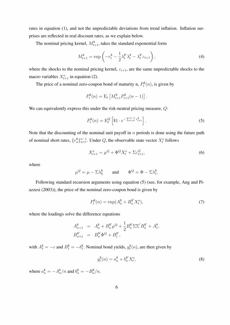
Following standard recursion arguments using equation (5) (see, for example, Ang and Pi-

azzesi (2003)), the price of the nominal zero-coupon bond is given by

P $t (n) = exp(A$

n +B$′

n Xot ), (7)

where the loadings solve the difference equations

A$n+1 = A$

n +B$′

n µQ +

1

2B$′

n ΣΣ′B$′

n + A$1,

B$′

n+1 = B$′

n ΦQ +B$′

1 ,

with A$1 = −c and B$

1 = −δ$1 . Nominal bond yields, y$t (n), are then given by

y$t (n) = a$n + b$′

nXot , (8)

where a$n = −A$n/n and b$n = −B$

n/n.

6

When the macro variables are not priced, that is λ$0 = λ$

1 = 0, then the yield on a nominal

bond of maturity n is simply the average of future Fed Funds rates (ignoring the Jensen’s in-

equality term) as given by the Expectations Hypothesis. Priced macro factors enter into µQ and

ΦQ causing the risk-neutral dynamics to differ from the process of Xot in the physical measure.

The resulting effects on the loadings A$n and B$

n are able to capture a constant risk premium and

time-varying risk premium, respectively, in the dynamics of nominal yields, as shown by Dai

and Singleton (2002), and others.

2.3 Inflation

We assume that observed inflation rates, πt, are a noisy realization of trend inflation at the

beginning of the period, πet−1:

6

πt = πc + πet−1 + Σπ′

εt + σπεπt . (9)

Ignoring the constant πc, which matches the mean of inflation as the state variables are de-

meaned, realized inflation, πt, is equal to trend inflation at the beginning of the period, πet−1,

plus an inflation shock, Σπ′εt + σπε

πt , where επt ∼ i.i.d. N(0, 1) is orthogonal to the factor

shocks, εt. The inflation surprise correlated with shocks to the state variables Xot are spanned

by nominal bonds while the inflation-specific shock, επt , is completely hedged only by real

bonds, as we now explain.

2.4 Real Short Rates

We denote the real pricing kernel, which prices real claims, as M rt+1. The real and nominal

kernels are linked through realized inflation. Denoting the logs of the real and nominal pricing

kernels as mrt and m$

t , respectively, the log of the real stochastic discount factor is equal to the

log of the nominal stochastic discount factor plus inflation:

mrt+1 = m$

t+1 + πt+1, (10)

6 Equation (9) assumes that trend inflation is an unbiased estimate of actual inflation. This is true in data. A

regression of future realized inflation over the next quarter on trend inflation, which is the median one-quarter

ahead inflation forecast from the Survey of Professional Forecasters, produces a coefficient on trend inflation of

0.86 with a robust standard error of 0.05. If the year-on-year quarterly change in realized inflation is used as the

regressand, the coefficient on trend inflation is 1.11 with a robust standard error of 0.04. In both cases, we fail to

reject that trend inflation is an unbiased predictor of future realized inflation at the 95% level.

7

where mrt+1 ≡ lnM r

t+1 and m$t+1 ≡ lnM$

t+1. The conditional expected value and conditional

volatility of both sides of equation (10) must coincide in order to prevent arbitrage. Thus, M rt+1

also takes a standard exponential form:7

M rt+1 = exp

(−rt −

1

2λr′

t λrt − λr′

t εt+1 + σπεπt+1

), (11)

where rt is the real short rate and λrt = λr

0 + λr1X

ot is the 3 × 1 column vector of real market

price of risk with λr0 a 3× 1 vector and λr

1 a 3× 3 vector.

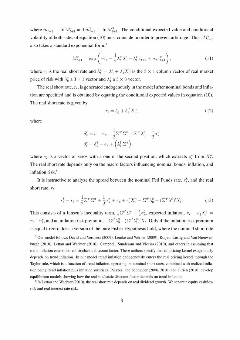
The real short rate, rt, is generated endogenously in the model after nominal bonds and infla-

tion are specified and is obtained by equating the conditional expected values in equation (10).

The real short rate is given by

rt = δr0 + δr′

1 Xot , (12)

where

δr0 = c− πc −1

2Σπ′

Σπ + Σπ′λ$0 −

1

2σ2π

δr1 = δ$1 − e2 +(λ$′

1 Σπ),

where e2 is a vector of zeros with a one in the second position, which extracts πet from Xo

t .

The real short rate depends only on the macro factors influencing nominal bonds, inflation, and

inflation risk.8

It is instructive to analyze the spread between the nominal Fed Funds rate, r$t , and the real

short rate, rt:

r$t − rt =1

2Σπ′

Σπ +1

2σ2π + πc + e′2X

ot − Σπ′

λ$0 − (Σπ′

λ$1)

′Xt. (13)

This consists of a Jensen’s inequality term, 12Σπ′

Σπ + 12σ2π, expected inflation, πc + e′2X

ot =

πc+πet , and an inflation risk premium, −Σπ′

λ$0−(Σπ′

λ$1)

′Xt. Only if the inflation risk premium

is equal to zero does a version of the pure Fisher Hypothesis hold, where the nominal short rate7 Our model follows David and Veronesi (2009), Lemke and Werner (2009), Koijen, Lustig and Van Nieuwer-

burgh (2010), Lettau and Wachter (2010), Campbell, Sunderam and Viceira (2010), and others in assuming that

trend inflation enters the real stochastic discount factor. These authors specify the real pricing kernel exogenously

depends on trend inflation. In our model trend inflation endogenously enters the real pricing kernel through the

Taylor rule, which is a function of trend inflation, operating on nominal short rates, combined with realized infla-

tion being trend inflation plus inflation surprises. Piazzesi and Schneider (2006, 2010) and Ulrich (2010) develop

equilibrium models showing how the real stochastic discount factor depends on trend inflation.8 In Lettau and Wachter (2010), the real short rate depends on real dividend growth. We separate equity cashflow

risk and real interest rate risk.

8

equals the real short rate plus expected inflation. If λ$1 = 0 and/or λ$

0 = 0, then there are risk

premiums on output, trend inflation, and monetary policy, which are reflected in the spread

between the overnight real short rate and the nominal Fed Funds rate. Equation (13) shows that

these risk premium adjustments are potentially important; empirically the real short rate is not

observed, but using the model we can infer real short rates from the nominal Fed Funds rate and

inflation given the prices of risk.

In equation (11), the real kernel, M rt+1, depends explicitly on inflation shocks, επt+1, but

inflation shocks do not enter the nominal kernel in equation (4). In the Taylor rule (1), the

Fed responds to trend inflation, not realized inflation. This corresponds to Fed practice in con-

centrating on forward-looking inflation measures and preferring to use core inflation, which

excludes relatively volatile food and energy prices, as its main inflation measure. A temporary

inflation shock leaves the Fed Funds rate unchanged, hence lowering its implied real payoff.

From equation (13), the real short rate remains unchanged but the inflation adjusted real short

rate increases by the temporary inflation shock.9 Thus, temporary inflation shocks are hedged

by investments in real bonds. The investor is willing to pay a positive premium to hedge expo-

sure to temporary inflation shocks, which are not reflected in the nominal Fed Funds rate. In

equation (11), the premium for this inflation hedge is −σπ per unit of inflation.

2.5 Real Bonds

We define a real zero-coupon bond as a security where the face value is indexed to the price in-

dex, or the payoff is constant in real terms. The nominal payoffs of real bonds depend explicitly

on the path of realized inflation. The yields of these bonds constitute the term structure of real

rates.

From equation (10), the real and nominal market prices of risk are linked by

λr0 = λ$

0 − Σπ and λr1 = λ$

1, (14)

where λrt = λr

0+λr1X

ot . The real and nominal prices of risk differ by the covariation of inflation

with the state variables, λrt = λ$

t − Σπ because our VAR in equation (2) is homoskedastic.

The real bond price of maturity n, P rt (n), satisfies the Euler equation

P rt (n) = Et[M

rt+1P

rt+1(n− 1)],

9 This is consistent with Treasury Inflation Protected Securities (TIPS) in the U.S. that pay out the real interest

rate plus realized inflation.

9

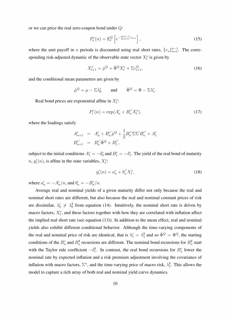
or we can price the real zero-coupon bond under Q:

P rt (n) = EQ

t

[e−

∑n−1i=0 rt+i

], (15)

where the unit payoff in n periods is discounted using real short rates, {ru}n−1u=t . The corre-

sponding risk-adjusted dynamic of the observable state vector Xot is given by

Xot+1 = µQ + ΦQXo

t + ΣεQt+1, (16)

and the conditional mean parameters are given by

µQ = µ− Σλr0 and ΦQ = Φ− Σλr

1.

Real bond prices are exponential affine in Xot :

P rt (n) = exp(Ar

n +Br′

n Xot ), (17)

where the loadings satisfy

Arn+1 = Ar

n +Br′

n µQ +

1

2Br′

n ΣΣ′Br′

n + Ar1

Br′

n+1 = Br′

n ΦQ +Br′

1 ,

subject to the initial conditions Ar1 = −δr0 and Br

1 = −δr1. The yield of the real bond of maturity

n, yrt (n), is affine in the state variables, Xot :

yrt (n) = arn + br′

nXot , (18)

where arn = −Arn/n, and brn = −Br

n/n.

Average real and nominal yields of a given maturity differ not only because the real and

nominal short rates are different, but also because the real and nominal constant prices of risk

are dissimilar, λr0 = λ$

0 from equation (14). Intuitively, the nominal short rate is driven by

macro factors, Xot , and these factors together with how they are correlated with inflation affect

the implied real short rate (see equation (13)). In addition to the mean effect, real and nominal

yields also exhibit different conditional behavior. Although the time-varying components of

the real and nominal price of risk are identical, that is λr1 = λ$

1 and so ΦQ = ΦQ, the starting

conditions of the Brn and B$

n recursions are different. The nominal bond recursions for B$n start

with the Taylor rule coefficient −δ$1 . In contrast, the real bond recursions for Brn lower the

nominal rate by expected inflation and a risk premium adjustment involving the covariance of

inflation with macro factors, Σπ, and the time-varying price of macro risk, λ$1. This allows the

model to capture a rich array of both real and nominal yield curve dynamics.

10

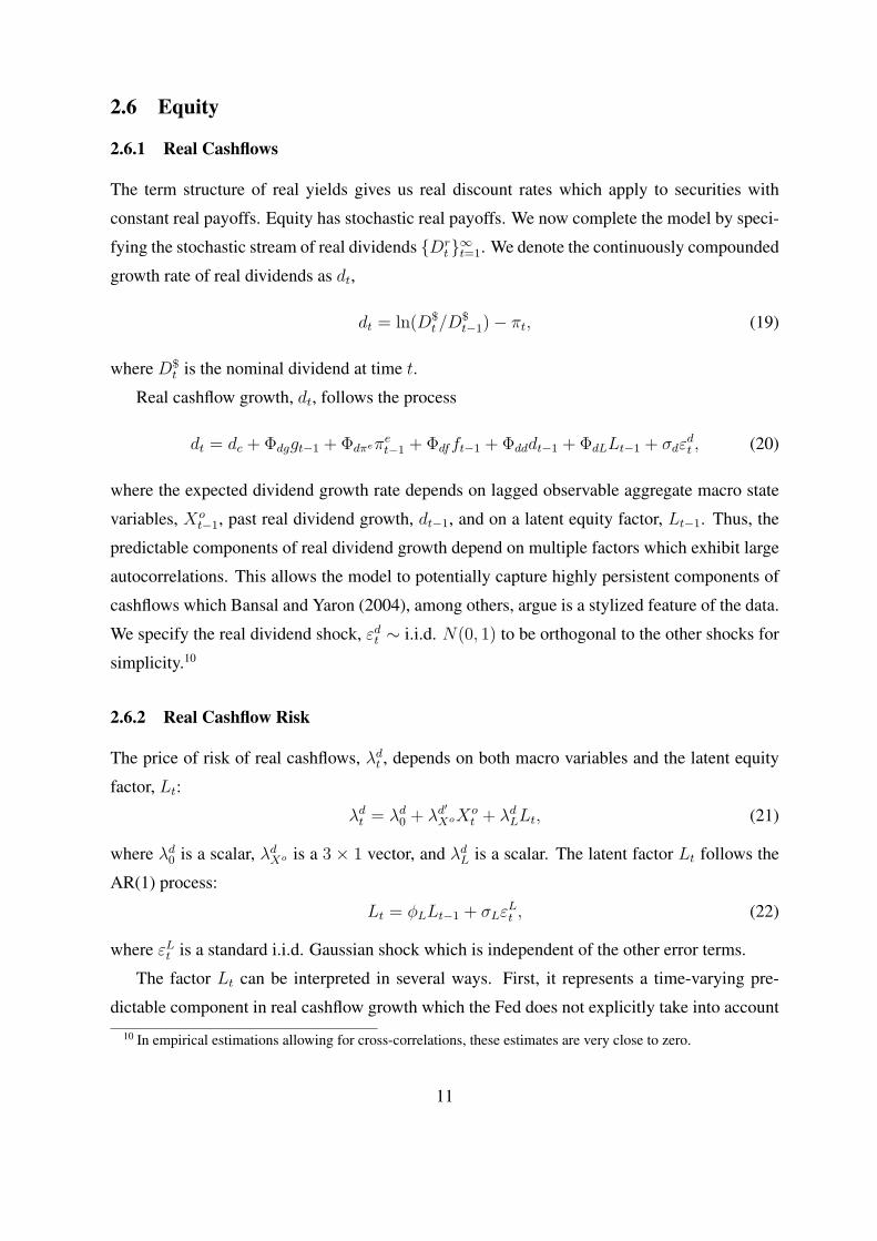
2.6 Equity

2.6.1 Real Cashflows

The term structure of real yields gives us real discount rates which apply to securities with

constant real payoffs. Equity has stochastic real payoffs. We now complete the model by speci-

fying the stochastic stream of real dividends {Drt }∞t=1. We denote the continuously compounded

growth rate of real dividends as dt,

dt = ln(D$t /D

$t−1)− πt, (19)

where D$t is the nominal dividend at time t.

Real cashflow growth, dt, follows the process

dt = dc + Φdggt−1 + Φdπeπet−1 + Φdfft−1 + Φdddt−1 + ΦdLLt−1 + σdε

dt , (20)

where the expected dividend growth rate depends on lagged observable aggregate macro state

variables, Xot−1, past real dividend growth, dt−1, and on a latent equity factor, Lt−1. Thus, the

predictable components of real dividend growth depend on multiple factors which exhibit large

autocorrelations. This allows the model to potentially capture highly persistent components of

cashflows which Bansal and Yaron (2004), among others, argue is a stylized feature of the data.

We specify the real dividend shock, εdt ∼ i.i.d. N(0, 1) to be orthogonal to the other shocks for

simplicity.10

2.6.2 Real Cashflow Risk

The price of risk of real cashflows, λdt , depends on both macro variables and the latent equity

factor, Lt:

λdt = λd

0 + λd′

XoXot + λd

LLt, (21)

where λd0 is a scalar, λd

Xo is a 3 × 1 vector, and λdL is a scalar. The latent factor Lt follows the

AR(1) process:

Lt = ϕLLt−1 + σLεLt , (22)

where εLt is a standard i.i.d. Gaussian shock which is independent of the other error terms.

The factor Lt can be interpreted in several ways. First, it represents a time-varying pre-

dictable component in real cashflow growth which the Fed does not explicitly take into account

10 In empirical estimations allowing for cross-correlations, these estimates are very close to zero.

11

in its policy rule. This could be technological change, for example, of the sort modeled by

Pastor and Veronesi (2009) that affects equity cashflows, but not bond yields. More broadly,

Lt captures any effect on equity cashflows and risk not captured by output, trend inflation, and

monetary policy.

From equation (21), Lt can be interpreted as a time-varying price of risk factor for real

dividends. In equation (21), the equity risk premium has two components: the first is due to

observable macro factors, Xot , and the second is driven by the equity factor, Lt. The factor

Lt enters the time-varying price of dividend growth risk and represents a priced risk premium

factor through the pricing of cashflow risk.11 Note we do not price Lt itself: this makes our

model similar to structural models like Campbell and Cochrane (1999) where factor risks in

equity are priced through their covariation with cashflows. An alternative interpretation is that

Lt captures a preference or sentiment shock affecting equities, and we investigate this in our

empirical work.

Similar to Brennan, Wang and Xia (2004) and Lettau and Wachter (2007), the latent price of

risk follows an AR(1) process in equation (22), but we allow it to also affect future cashflows.

This potentially captures the predictability of dividend growth by components that also drive

expected returns, like the Lt process, consistent with Lettau and Ludvigson (2005) and Ang and

Bekaert (2007). We identify Lt through its impact on the cashflow process and the dividend

yield. Other studies like Brandt and Kang (2004) and Rytchkov (2010) estimate persistent un-

observable components of expected returns, except the latent components are identified with

realized return variation. Identifying persistent risk premium factors with cashflows and divi-

dend yields is more precise because returns are substantially more conditionally volatile than

dividend yields. Binsbergen and Koijen (2010) also estimate latent expected return factors from

price-dividend ratios, but they do not allow the risk premium factor to also influence cashflows,

through ΦdL, or account for the effect of macro risk through Xot .

Finally, Lt can be econometrically viewed as a “goodness-of-fit” test of the ability of Xot

to explain equity prices by comparing an estimation without Lt to an estimation with only

observable macro factors and cashflows. A large discrepancy between the two models may

indicate model mis-specification or that the required variation in equity risk premiums cannot

be captured by variations in our observed aggregate macro factors Xot . We examine estimations

11 We do not allow the market price of real cashflow risk to depend on real dividend growth dt. An unexpected

change in real dividend growth, as reflected by a change in dt, changes the cashflow but not the premium for

cashflow risk. Thus, dt has a pure interpretation of being a cashflow factor and its time-varying price of risk

depends on Lt.

12

with and without Lt in our empirical work and show that the observed aggregate macro factors

Xot alone account for most of the variation in dividend yields.

2.6.3 Equity Prices

Under no arbitrage, the price of a stock equals the risk-neutral expected value of future real

dividends, discounted by real short rates:12

P rt

Drt

=P $t

D$t

= EQt

[∞∑s=1

exp

(s∑

k=1

dt+k − rt+k−1

)], (23)

where P rt /D

rt = P $

t /D$t is the price-dividend ratio in both real and nominal terms. In equa-

tion (23), the timing of the real dividend growth and real short rates are offset because the real

short rates are known at the beginning of the period.

To price equity, we collect the whole set of factors in Xt = (gt πet ft dt Lt)

′. We write the

dynamics of Xt compactly as a VAR(1):

Xt = µ+ ΦXt + Σεt+1, (24)

where εt+1 = (ε′t+1 εdt+1 ε

Lt+1)

′ and the parameters µ, Φ, and Σ are determined by stacking

equations (2), (20), and (22).

We define the prices of risk corresponding to Xt as

λt = λ0 + λ1Xt, (25)

where

λ0 =

λr0[3× 1]

λd0

0

and λ1 =

λr1 [3× 3] 0 [3× 2]

λd′Xo [1× 3] 0 λd

L

0 [1× 5]

,

where the dimensions of the matrices are given in square brackets and all other parameters are

scalars. Under the risk-neutral measure Q, the extended state vector that determines equity

prices, Xt, follows

Xt+1 = µQ + ΦQXt + ΣεQt+1,

where

µQ = µ− Σλ0 and ΦQ = Φ− Σλ1.

12 Alternatively, one can also discount the value of future nominal dividends by the nominal short rate under the

risk-neutral measure. Both approaches yield identical equity values.

13

Using standard techniques (see, for example, Ang and Liu (2001)), the price-dividend ratio

takes the formP rt

Drt

=P $t

D$t

=∞∑n=1

exp(an + b′nXt), (26)

where an and bn follow the recursions

an+1 = an − δr0 + (e4 + bn)′µQ +

1

2(e4 + bn)

′ΣΣ′(e4 + bn)

bn+1 = −δr1 + ΦQ′(e4 + bn),

where a1 = −δr0 + e′4µQ + 1

2e′4ΣΣ

′e4, b1 = −δr1 + ΦQ′e4, δr1 = (δr

′1 0 0)′ and e4 = (0 0 0 1 0)′.

The price-dividend ratio naturally depends on real cashflow growth, which enters the re-

cursions explicitly through the terms involving e4. It also depends on the state of the macro

economy, Xot , and the equity premium latent factor Lt. These factors affect both the forecasts

of future real cashflows, through Φ, and the time-varying price of risk of dividends, through λ1.

2.7 The Term Structures of Risk Premiums

The previous sections derived the prices of nominal bonds, real bonds, and equity. From these

prices, we now define and compute expected equity returns and equity risk premiums (see

Appendix A for analytical expressions).

We define the expected k-period total holding return on equity as

Et[RE,$t (k)] = Et

[ln

(P $t+1 +D$

t+1

P $t

)+ ...+ ln

(P $t+k +D$

t+k

P $t+k−1

)], (27)

where prices, P $, and dividends, D$, are in nominal terms. We also refer to this as the total

expected equity return. Varying maturity k, we have a term structure of expected equity returns.

The expected k-period real holding return on equity is defined as

Et[RE,rt (k)] = Et

[ln

(P rt+1 +Dr

t+1

P rt

)+ ...+ ln

(P rt+k +Dr

t+k

P rt+k−1

)], (28)

where all quantities are now real. The difference between the total and real expected holding

period returns is expected inflation, Et[πt(k)]:

Et[RE,$t (k)] = Et[R

E,rt (k)] + Et[πt(k)], (29)

where

πt(k) = πt+1 + ...+ πt+k

14

is the cumulative (log) inflation rate from time t to t+ k.

For a given horizon k, we can decompose the expected total equity return into several com-

ponents. We start with the real short rate, rt. Now consider a real zero-coupon bond with

maturity k. The real yield, yrt (k), is the expected holding period return on this bond from t to

t+k. This compensates the investor for real duration risk. Next, we could hold a nominal zero-

coupon bond of maturity k with yield y$t (k). The inflation risk present in this nominal bond

must be compensated in equilibrium by a higher real return. We define the expected real return

over k periods on a nominal zero-coupon bond of maturity k, y$,rt (k), as the nominal bond’s

holding period return (which is the same as the nominal bond yield) less expected inflation,

y$,rt (k) = y$t (k)−Et[πt(k)]. The difference between the real yield on the nominal bond and the

real bond represents an inflation risk premium. Finally, we have the expected nominal equity

return, Et[RE,$t (k)]. Real equity cashflows are stochastic, and so the difference between the

expected nominal equity return and the nominal bond yield represents a real cashflow premium.

We summarize this as:

Et[RE,$t (k)] = Et[R

E,rt (k)] + Et[πt(k)] Total equity return

= rt Real short rate, rt+ (yrt (k)− rt) Real duration premium, DPt(k)

+ (y$,rt (k)− yrt (k)) Inflation risk premium, IRPt(k)

+ (y$t (k)− y$,rt (k)) Expected inflation, Et[πt(k)]

+ (Et[RE,$t (k)]− y$t (k)) Real cashflow risk premium, CFPt(k)

Thus, we decompose the total expected equity return as:

Et[RE,$t (k)] = rt +DPt(k) + IRPt(k) + Et[πt(k)] + CFPt(k). (30)

Each of these risk premiums themselves have a term structure across horizons k. All of these

risk premiums also vary over time.

The cashflow risk premium, CFPt(k), can be interpreted as an “equity risk premium,” as

it is the difference between expected total equity returns and the expected return on a nom-

inal bond. Practitioners often use this definition (see, for example, Asness (2000); Ibbotson

and Chen (2003)), except they generally use yields on coupon bonds rather than zero-coupon

bonds.13 We prefer the more precise term “cashflow risk premium” to indicate that it is the in-

cremental reward for bearing stochastic dividend risk in excess of nominal bonds. The cashflow13 In contrast, many academics prefer to define the equity risk premium as the difference between total equity

returns and short rates (or cash returns), following Mehra and Prescott (1985).

15

premium is equivalently given by the difference between expected real equity returns and real

returns on nominal bonds:

CFPt(k) = Et[RE,$t (k)]− y$t (k) = Et[R

E,rt (k)]− y$,rt (k). (31)

We also refer to the cashflow risk premium as the “equity risk premium over nominal bonds.”

We define the “equity risk premium over real bonds” or the “real risk premium” as:

RRPt(k) = Et[RE,rt (k)]− yrt (k)), (32)

which is the difference between the expected real equity return and the real bond yield. The

difference between the nominal and real equity risk premiums is expected inflation plus the

inflation risk premium, Et[πt(k)] + IRPt(k). Put another way, the real risk premium is the sum

of the cashflow premium and the inflation risk premium:

RRPt(k) = CFPt(k) + IRPt(k). (33)

In our empirical work, we focus on the 10-year horizon (k = 40 quarters) for our bench-

mark results. This is a benchmark maturity in fixed income and is the horizon often chosen to

correspond to “long-term” forecasts in surveys (such as the Survey of Professional Forecasters

and surveys of industry professionals like Graham and Harvey (2005), for example). But, we

also consider the term structure of risk premiums over various k.

3 Data

We work at the quarterly frequency and take data from 1982:Q1 to 2008:Q4. Over 1979-1982

the Fed set explicit targets for monetary aggregates and so we start our estimation in 1982:Q1 to

avoid this period. The sample on real bonds starts later in 2003:Q1 due to the non-availability

and liquidity problems of real bonds in the earlier part of the sample.

We take the output gap for gt, the median one-quarter ahead inflation forecast from the

Survey of Professional Forecasters (SPF) for πet , and construct ft as the residual from the Taylor-

rule regression (1) for ft. The inflation rate, πt, is the change in the consumer price index over

the past year. Ang, Bekaert and Wei (2007) show that the median inflation forecast from the

SPF has the best performance for forecasting inflation among a comprehensive collection of

Phillips curve models, time-series models, and macro term structure models.

Figure 1 plots the output gap, trend inflation, and the monetary policy shock. All variables

are demeaned. The output gap, gt, has decreased in all recessions and reaches its lowest point

16

during the 2008 recession (the “Great Recession”). Trend inflation, πet , has become less volatile

since the early 1990s, as documented by Clark and Davig (2009), and others, but remains an-

chored to the end of the sample. Both gt and πet are highly persistent with autocorrelations of

0.97 and 0.92, respectively. The monetary policy shock, ft, is the least persistent process, with

an autocorrelation of 0.52, and reaches its maximum during the 1987 Savings and Loan crisis

and its minimum during the 1991 recession.

The bond data comprise the Fed Funds rate, nominal bond yields, and real bond yields. All

bond yields are expressed as continuously compounded rates. We take zero-coupon bonds for

nominal and real bonds from the Board of Governors of the Federal Reserve System, which

are constructed following the method of Gurkaynak, Sack and Wright (2007, 2010). We take

nominal bonds of maturities 1, 3, 5, 7, 10, 12, and 15 years. We deliberately do not take the very

long part of the term structure (the 30-year maturity) because of the repurchase of long-dated

bonds and the temporary cessation of the issue of 30-year bonds during the early 2000s due to

Federal government surpluses at that time.

The data on real zero-coupon bonds are constructed from TIPS and we take maturities of 5,

7, 10, 12, and 15 years starting in 2003:Q1. Although the first TIPS were issued in 1997, the

TIPS market was very illiquid for the first few years. We take data starting 2003:Q1 to mitigate

these effects (see, among others, D’Amico, Kim and Wei (2007); Pflueger and Viceira (2011)).

We do not take short maturity TIPS as these are only available later in the sample and require

adjustments for indexation lags and the deflation put.14 For this reason, we take only horizons

greater than five years when we discuss the real duration premium, DPt(k), and the real equity

risk premium, RRPt(k).

Equity dividend yields are constructed using the CRSP value-weighted stock index. We

construct dividend yields by summing dividends over the past four quarters to remove seasonal-

ity. Our year-on-year real dividend growth rates at the quarterly frequency are also constructed

to remove seasonality. Appendix B contains further details on the data.

14 While most analysis with TIPS does not take into account indexation lags, Evans (1998) considers indexation

lags for UK real bonds. His analysis does not find evidence that the indexation lag affects market prices signifi-

cantly. The deflation put refers to the property of TIPS where the principal does not fall below par when inflation

is negative (see, for example, Jacoby and Shiller (2008)).

17

4 Empirical Results

4.1 Parameter Estimates

We report the parameter estimates of the model in Table 1.15 The top panel reports estimates

of the Taylor rule (equation (1)) and shows that the Fed responses on the output gap and trend

inflation are 0.31 and 2.44, respectively, with both coefficients being highly significant. These

signs are consistent with those in the literature where the Fed lowers the Fed Funds rate in

response to weakening economic growth and raises the Fed Funds rate when inflation expecta-

tions increase. The reaction of the Fed to trend inflation is very strong at 2.44. This is consistent

with Clarida, Galı and Gertler (2000), Boivin (2006), Ang et al. (2011), and others, who find

that the response of the Fed to inflation since the post-Volcker era has been, on average, much

larger than one. These and other studies, however, generally find lower coefficients than 2.44

because they tend to use realized inflation, rather than trend inflation as we do. The R2 of this

regression is 70%, so the policy rule explains a large amount of the variation in the Fed Funds

rate.

As expected, the VAR dynamics in Table 1 (equations (2), (20), and (22)) reflect the high

persistence in the output gap and trend inflation (see Figure 1). The latent factor is less persistent

with ϕL = 0.16. There is evidence of Granger-causality in both directions between the output

gap and trend inflation, where increases in either variable predict increases in the other variable

next period. The real cashflow equation shows that all variables, including lagged cashflows,

predict next-period real cashflows. Increases in trend inflation Granger-cause large decreases

in future real dividend growth, with a coefficient of -2.45. This is consistent with a large liter-

ature in macroeconomics finding that inflation is negatively related with real production (see,

for example, Fama (1981)). Empirically, nominal price rigidity is pervasive as Nakamura and

Steinsson (2008) show and cost increases can only be passed on in stages, rather than continu-

ously. In models like Diamond (1993), menu costs reduce market power as consumers search

for products which have not had price increases. Thus, rising inflation reduces profit margins

and consequently reduces real payouts. In the equation for dt, real dividend growth also de-

creases with positive Fed policy surprises, with a coefficient of -0.21. Thus, active monetary

policy that is more aggressive than implied by the Taylor rule further stifles real equity cash-

flows.15 Details of the estimation are in Appendix C.

18

4.2 Real and Nominal Short Rates

Real short rates are empirically unobserved, but endogenously determined in the model. Real

short rate dynamics follow:

rt = 0.0074 + 0.1993 gt + 1.7112 πet + 1.3547 ft,

(0.0015) (0.3334) (0.2652) (0.0697)(34)

with standard errors in parentheses. In the nominal Taylor rule, the coefficient on trend inflation,

πet , is 2.44 (see Table 1). In equation (34), the coefficient on πe

t is 1.71 and thus the real rate is

not simply the nominal rate minus trend inflation as per the Fisher relation. Non-neutrality arises

from three sources. First, the Fed is very aggressive in the nominal Taylor rule (equation (1)),

with a response to πet well above one. This causes the real rate loading on πe

t to be greater than

zero. In fact, the coefficient on πet is a very large 1.71 indicating that increases in trend inflation

coincide with more than one-for-one increases in real rates. This finding is consistent with

Woodford (2003) and others who argue that the Fed tries to affect real interest rates through

active nominal interest rate policies.

If the real rate were simply the nominal rate less trend inflation, the coefficient on πet should

simply be 2.44− 1 = 1.44. In our model, the real rate coefficient on πet is 1.71, which is higher

than 1.44 due to the inflation risk premium (see equation (13)). Monetary policy moves both

the real rate, with a coefficient of 1.35, more than it moves the nominal rate, where ft has a

coefficient of one by definition, due to the price of real rate risk. Thus, monetary policy actions

taken by the Fed have a larger effect in real versus nominal terms.

The instantaneous inflation risk premium, IRPt(k = 0), using the notation in equation (30)

is the difference between the Fed Funds rate, r$t , and the sum of the real short rate and trend

inflation, rt + πet :

IRPt(0) = r$t − (r + πet ).

Substituting the Taylor rule and the real short rate in equation (34), the inflation risk premium

associated with the Fed Funds rate is given by:

IRPt(0) = 0.0075 + 0.1141 gt – 0.2757 πet – 0.3455 ft,

(0.0016) (0.3689) (0.2733) (0.0697)(35)

with standard errors in parentheses. We fail to reject that the Fed Funds inflation risk premium

does not respond to output gap and trend inflation shocks. On the other hand, the coefficient on

ft in equation (35) is significantly negative. One economic reason for the Fed Funds inflation

19

risk premium to decrease with tighter monetary policy may be that agents expect Fed actions to

be successful at combating inflation risk (see, for example, Ulrich (2011b)).

Figure 2 plots the real short rate implied by the model, rt, and the Fed Funds rate, r$t . In

periods where trend inflation is stable and the output gap is low, the Fed can set real rates to be

negative by setting the Fed Funds rate to be lower than predicted by the Taylor rule (so there

are negative monetary policy shocks). The real short rate is negative during the 1991, 2001,

and 2008 recessions, and bottoms at -1.81% during the 2008 financial crisis. This reflects the

Fed’s strategy of aggressively lowering the Fed Funds rate to low levels when the economy is in

recession, even if trend inflation is positive, producing negative real short rates. There is a high

correlation between rt and r$t of 0.95. The real short rate has been, on average, 2.98% lower

than the Fed funds rate. This difference reflects the sum of trend inflation and the time-varying

inflation risk premium (see equation (13)). The smallest difference between the real rate and

nominal rate is 0.34% in 1986:Q4, which corresponds to the largest deviation from the Taylor

rule in our data sample.

4.3 The Term Structure of Nominal and Real Bonds

Figure 3 plots the model-implied average nominal yield curve and for comparison the average

yields, with two standard error bounds, in data. Like most affine models fitted on nominal

yield curve data, the fit is excellent. However, while most term structure models require latent

factors to fit the yield curve well, our model closely matches nominal yield curves with only

observable factors. In the level and slope principal component interpretation of Litterman and

Scheinkman (1991), trend inflation, πet , tracks the level of the yield curve well and the monetary

policy factor, ft, closely matches the slope factor. Long-term bond yields are very sensitive to

trend inflation. In particular, the 10-year nominal bond yield in our model can be written as

y$t (10 yrs) = 0.0177 + 0.1969gt + 2.0009πet + 0.2739ft, (36)

which demonstrates the large sensitivity of nominal bonds to variation in expected inflation. As

trend inflation increases the inflation risk premium increases, and agents demand higher yields

on long-term bonds to compensate for the higher inflation risk premium.

In Figure 4, we plot the term structure of real yields implied by the model and the average

real yields in data, with two standard error bounds. The model-implied curve lies between two

standard deviation bounds for all yields except the 60-quarter maturity. The inferior, but still

relatively good, fit to the real yield curve compared to the nominal yield curve in Figure 3 is due

20

largely to the shorter estimation period for real bonds, 2003:Q1-2008:Q4, compared to the full

sample which starts in 1982:Q1. Note that TIPS are well known to have significant liquidity

effects even over the post-2003 sample, as documented by D’Amico, Kim and Wei (2008) and

Pflueger and Viceira (2011), among others. Our model does not incorporate an extra liquidity

factor to fit the TIPS curve, as D’Amico, Kim and Wei do, and uses the same factors to fit both

the nominal and real curves. In this light, the fit to the real yield curve is excellent.

The bottom panel of Figure 4 shows the model-implied real yield term structure interpolated

for the full sample. The real term spread between the 60-quarter and 20-quarter maturities is

0.74%.16 Our model produces both an upward-sloping nominal and real yield curve through

the positive risk premiums for the output gap and inflation. Economically, the positive real

term spread can reflect, among other things, consumption growth risk (see Wachter (2006)) or

uncertainty about the effectiveness of benevolent government interventions in the business cycle

(see Ulrich (2011b)).

4.4 Equity

Figure 5 graphs dividend yields. We plot the model-implied dividend yield without the latent

factor, Lt, in the dashed line, and the dividend yield in data in the solid line. By construction,

we obtain an exact match with the dividend yield in data with Lt. Impressively, the model is

able to match closely the dividend yield in data without Lt. To gain some intuition on how

the model matches dividend yields, we can interpret the loadings on the various factors in the

log-linearized dividend yield:

ln

(1 +

Dt

Pt

)≃ 0.0063− 0.0149gt + 0.7976πe

t − 0.0185ft − 0.0022dt + 0.0094Lt. (37)

Note that the dividend yield is countercyclical. In equation (37), the negative loading on the

output gap, gt, and real dividend growth, dt, indicates that in expansions gt and dt are high,

expected returns are low and prices are high, and thus dividend yields are low.

The high correlation between dividend yields and long-term bond yields in data is often

called the “Fed model”. In our sample, the correlation between the dividend yield and the 10-

year nominal bond yield is 0.87, which our model matches exactly. In equation (37) there is

16 Ang, Bekaert and Wei (2008) estimate real yield curves over earlier periods when TIPS are not traded and find

that the real yield curve is fairly flat. They do not use traded TIPS and their ending maturity is 20 quarters, which

is the first maturity of our real bonds in data.

21

a large coefficient of 0.80 on trend inflation, πet . Trend inflation has the largest effect on divi-

dend yields of all the variables. An increase in trend inflation decreases real cashflow growth,

increases the real interest rate, the inflation risk premium, and the cashflow premium. This

decreases equity prices and increases dividend ratios. Long-term bonds are highly sensitive to

variation in trend inflation as well (see equation (36)). Thus, an increase in trend inflation simul-

taneously increases yields on bonds and the dividend yield. The correlation of trend inflation

with the 10-year nominal bond is 0.95 and the correlation of trend inflation with the dividend

yield is 0.91 implied by the model. These are very close to their counterparts in data, which are

0.88 and 0.91, respectively.

In equation (37), the negative coefficient on ft implies that a surprise move by the Fed to

inject liquidity beyond that suggested by the Taylor rule (a negative ft shock) increases dividend

yields. Thus, a surprise loosening of monetary policy tends to decrease stock prices and increase

dividend yields. This is due to the effect of monetary policy surprises on real dividend risk.

While surprise decreases in the Fed Funds rate spur, on average, increases in real dividends

next period, which we see by the coefficient Φdf = −0.21 in equation (20) and reported in

Table 1, the price of risk of cashflow growth increases, as λdf is negative. Surprise decreases,

therefore, in the Fed Funds rate increase equity cashflows, but these cashflows are discounted

at higher rates. The discount rate effect dominates and this causes the dividend yield to rise.

On the other hand, during recessions gt is low and πet is low, so the Fed Funds rate, r$t , falls as

predicted by the Taylor rule. A negative surprise in ft sends r$t lower than implied by the Taylor

rule. In our model this is risky, and the discount rate increases to reflect that risk.

4.4.1 Latent Equity Factor

When Lt is included, we match the dividend yield exactly so Lt is a non-linear function of the

difference between the dividend yield implied by the model and the actual dividend yield in

data in Figure 5. From equation (37), high Lt causes low equity prices, or high dividend yields.

The correlation between dividend yields and Lt is 0.46.

We investigate if movements in Lt reflect factors not captured in the model, especially credit

risk, volatility risk, sentiment, and liquidity. We measure credit risk by the Baa-Aaa credit

spread, volatility risk as the VIX volatility index, sentiment by the Baker and Wurgler (2007)

sentiment factor, and take the liquidity factor from Pastor and Stambaugh (2003). In Table 2,

we run contemporaneous regressions of Lt onto these various factors. In regressions I-IV, we

consider univariate relations. The latent equity factor Lt has the strongest relation with the

22

Baker-Wurgler sentiment factor, with a t-statistic of -5.42 and an adjusted R2 of 28%. Thus,

Lt, which represents the portion of equity price movements not captured by macro variables

and cashflows, can be interpreted partly as a sentiment factor in line with Baker and Wurgler.

In fact, this is the only factor that exhibits a significant correlation with Lt. It remains the only

significant relation in the joint regression V. In regression VI where we add controls for macro

variables, both sentiment and trend inflation carry significant loadings.

Figure 6 plots Lt together with the Baker-Wurgler sentiment factor. Periods of low sentiment

tend to coincide with periods of high Lt and vice versa. The sentiment factor reaches a sharp

peak in 2001:Q1 where equity prices are very high. While the equity factor Lt is low during

this period, the low values of Lt are not unusual. During this time, the output gap is high

and inflation expectations are low, as shown in Figure 1. This causes both interest rates and

discount rates to be low, leading to macro-based equity prices to be very high. Thus, the model

accounts for low dividend yields in the late 1990s and early 2000s by low macro risk similar

to Lettau, Ludvigson and Wachter (2008), rather than an unusual increase in sentiment. In

contrast, Shiller (2000) and Baker and Wurgler (2007), among others, attribute low dividend

yields during this time almost entirely to high sentiment.

4.5 The Term Structure of Equity Risk Premiums

We now decompose the total equity return into various risk premium components following

Section 2.7. We start by examining the total expected return, Et[RE,$t (k)], the cashflow risk

premium, CFPt(k) (the equity risk premium over nominal bonds), and the real risk premium,

RRPt(k) (the equity risk premium over real bonds), in Figure 7. As we vary the horizon, k, we

trace out the term structure of total equity returns and equity risk premiums. As our starting real

bond in data has a maturity of 20 quarters, we start the real risk premium curve at this maturity.

We end at 60 quarters, which is the longest maturity of both nominal and real bonds in data.

Figure 7 shows that the term structure of total equity returns is downward sloping. The

downward-sloping curve implies that equity becomes less risky, or that total expected holding

period returns decrease, as the horizon increases. Similar downward-sloping term structures

have been estimated by Lettau and Wachter (2010), Binsbergen, Brandt and Koijen (2011), and

Binsbergen et al. (2011), among others. At a one-year horizon, the total expected equity return

is 12.6% and this reduces to 11.0% for the 15-year horizon. Using the joint term structures

of nominal and real bonds, we plot the cashflow risk premiums and real risk premiums in the

dotted and dotted-dashed lines, respectively. Figure 7 shows that the cashflow risk premium has

23

a similar downward-sloping pattern, decreasing from 6.7% at the one-year horizon to 3.9% at

the 15-year horizon. The real risk premium is also sloped downwards, with real risk premiums

of 4.5% and 4.4% at the five and 15-year horizons, respectively.

The term structure of equity returns is downward sloping due to the risk premium associated

with expected inflation decreasing with horizon. Intuitively, equity in the long run has some

inflation-hedging ability as its risk premium with respect to trend inflation falls. The risk due

to the output gap and monetary policy shocks increases with maturity. The monetary policy

shock is quickly mean-reverting, so it lowers the cashflow premium at small horizons and has

effectively no effect on horizons greater than five quarters. The offsetting effects of the falling

inflation premium and the increasing output gap premium, combined with the very short-acting

monetary policy shock premium, contribute to the small hook in the term structure of expected

returns at short horizons. In the long run, the decreasing trend inflation risk premium dominates,

and equity becomes less risky at longer horizons.

4.6 Decomposing Equity Risk Premiums

We can further decompose the total expected return into the real return, real duration premiums,

expected inflation and inflation risk premiums, and the cashflow premium. This is done in

Figure 8 and Table 3. Panel A of Table 3 reports the unconditional risk premiums. The real

short rate implied by the model is 2.98%, on average. The reward for bearing real duration

risk is very small at 0.1% at the five-year horizon increasing to 0.81% at the 15-year horizon.

Expected inflation is approximately 3%. The inflation risk premium, which is the difference

between nominal and the Fisher Hypothesis-implied real bond yields, is slightly upward sloping

past the five-year horizon and increases from 0.41% to 0.62% from five to 15 years. While these

real duration and inflation risk premiums are increasing, the cashflow premium is decreasing

across horizon. This makes the overall expected total return curve downward sloping.

Panel B of Table 3 reports a variance decomposition of the total expected equity return. At

the 10-year horizon, there is substantial variation due to the real rate, with a variance decompo-

sition of 37%. In our model, the real rate is a function of macro factors and these same macro

factors also drive expected equity returns. Real duration risk accounts for 18% of the variance.

The contribution from expected inflation and the inflation risk premium is negligible. Finally,

the variation in the cashflow premium accounts for 43% of variance in total expected equity

returns. Hence, most of the contribution of the total expected return comes from real rates and

cashflow risk premiums. Whereas the variance attributions of the real rate increase from 19% to

24

44% from five to 15 years, the variance attributions of the cash flow risk premium decrease from

72% to 32% over those horizons. Thus, cashflow risk premiums drive most variation of total

expected equity returns at short horizons while real rate variation dominates at long horizons;

in this sense, equity, in the long run, is a real security.

The difference between the equity risk premium over nominal bonds, CFP , and the equity

risk premium over real bonds, RRP , is the inflation risk premium, IRP (see equation (33)).

Table 3 reports that the cashflow premium and the real risk premium are very similar because

the inflation risk premium is modest. At the 10-year horizon, the cashflow premium is 3.84%

and the real risk premium is 4.45%, implying a 10-year inflation risk premium of 0.60%. The

inflation risk premium does not exhibit much variation as a proportion of the variation of the

expected total equity return, with a variance decomposition of approximately 1% at the 10-year

horizon. This is why the variance decomposition of the expected equity return into the cashflow

premium and the real risk premium components are very similar at around 43-44%.

In Table 4, we report various correlations of the risk premiums and macro factors. The risk

premiums are all computed at the 10-year horizon. There are several notable relations. First,

the real short rate is strongly negatively correlated with the real duration premium, at -90%.

Furthermore, the real duration premium has the highest correlation in absolute value with the

Fed monetary policy shock with a correlation of -100%. This is consistent with the Fed lowering

the real short rate through negative monetary policy shocks during recessions when the duration

premium is the steepest.

Second, the real inflation risk premium is pro-cyclical and and has an 80% correlation with

the real short rate and a 94% with the nominal Fed Funds rate. Of the macro variables, the

output gap and the monetary policy shock have the highest correlations with the inflation risk

premium, with correlations of 100% and -46%, respectively. This is intuitive as an increase in

the output gap signals an overheating of the economy which leads to inflation pressure, while a

boost in liquidity (negative ft shock) raises concerns about future inflation. These effects cause

the inflation risk premium to increase.

Third, trend inflation and the latent equity factor have the highest correlations with the real

cashflow premium, with correlations of 100% and 58%, respectively. The strong co-movement

with trend inflation shows the importance of trend inflation as a macro risk-factor for equity.

Investors are sensitive to variations in trend inflation and require substantial premiums for all

assets that do not perfectly hedge these shocks. The time variation of the ten-year cash-flow

premium arises mainly from the predictability of trend inflation. The same conclusions hold for

25

the ten-year real risk premium, because the much larger and more volatile cashflow premium

dominates the inflation risk premium.

Finally, the total 10-year expected equity return correlates strongly with the real short rate,

at 42%. This noteworthy correlation is driven by the relation between the output gap and trend

inflation with equities, which have correlations with the time-varying 10-year total equity return

of 70% and 84%, respectively. The correlation with the volatile equity specific latent factor is

51%. These results demonstrate that the variation in long-horizon equity returns arises from

underlying variations in the output gap and trend inflation.

How much of the variance of the risk premiums can we attribute to the macro and other

factors? We answer this in Table 5 by computing factor variance decompositions at the 10-year

horizon. Macro factors matter a lot for all premium components: the real short rate, real duration

premium, expected inflation, inflation risk premium, and the cashflow premium. For the real

short rate, trend inflation and monetary policy shocks account for 97% of variance. Monetary

policy actions are responsible for driving almost all variation in real duration premiums. Not

surprisingly, variation in expected inflation accounts for most of the variation in the inflation

risk premium.

For the 10-year equity risk premiums (the cashflow and real risk premiums) reported in

Table 5, economic growth dominates with variance decompositions above 60%. At longer

horizons, the effect of economic growth is even more important with the variance decomposition

at the 15-year horizon being over 70% for both the cashflow and real risk premiums. At long

horizons, trend inflation, monetary policy actions, and real dividend growth account for little

of the variation in equity risk premiums; we attribute the remainder of the variance in equity

risk premiums to the equity latent factor, Lt, but this effect is approximately half the effect of

economic growth. The output gap is a persistent process, with an autocorrelation of 0.9715:

long-run economic growth has the same effect as persistent long-run consumption growth in

the Bansal and Yaron (2004) setting and constitutes a long-run equity risk premium factor.

4.7 The Time Series of Risk Premiums

Figure 9 shows the time series of 10-year risk premiums. In Panel A, we graph the expected

total equity return (left-hand axis) along with the dividend yield (right-hand axis). As dividend

yields fall, total expected equity returns also decrease. Expected returns on equity are above

20% during the early 1980s and decrease through the 1980s and 2000s, reaching a low of 2.8%

during 2000:Q3. This is consistent with low equity returns as macroeconomic volatility declines

26

during the “Great Moderation” as noted by Lettau, Ludvigson and Wachter (2008). After this

low, the expected equity return increases during the 2001 recession and remains flat around 10%

during the mid-2000s. During the financial crisis expected returns on equity increase to 19% in

2008:Q4. The correlation between the expected 10-year total equity return and dividend yields

is 0.90, consistent with Campbell and Shiller (1988), Cochrane (1992), and others, who find

that discount rate variation accounts for a large fraction of dividend yield variation.

In Panel B, we break down the total expected equity return into its various components.

The real short rate is the same as Figure 2 and is included for completeness. The much lower

volatility, and lower average real short rate post the mid-1980s, reflects the Great Moderation.

The real duration premium exhibits pronounced swings and increases during every recession.

The real duration premium is negative in the early 1980s when real rates were high and volatile.

It reaches a low of -8% during the 1987 Savings and Loan crisis, turns positive in the early

1990s, and peaks at 5% during the 1991 recession. During the late 1990s, the real duration

premium is around zero, sharply increases during the 2000s recession, slowly falls below zero

before the on-set of the financial crisis, and during the financial crisis reaches 3% at 2008:Q4.

Economically, during recessions the market prices long-term real bonds with a large duration

premium to reflect the increased risk that economic growth is slow during these periods. The

duration premium correlates highly with monetary policy shocks (See Table 5), with a correla-

tion of -0.98. The duration premium is highest in recessions because the Fed tends to lower the

Fed Funds rates more aggressively than suggested by the Taylor rule during those times.

The next panel graphs the inflation risk premium and expected inflation. The 10-year ex-

pected inflation is fairly stable during the sample, and gradually falls from 3.6% at 1982:Q1 to

2.5% at 2008:Q4. The inflation risk premium reflects this gradual decrease in expected inflation.

The highest inflation risk premium occurs at the beginning of the sample at 2.4% in 1982:Q1.

It is relatively volatile during the 1980s, which reflects the higher volatility of inflation and the

real short rate at this time (see also Figure 1). Since 1992, the inflation risk premium has been

close to zero. It is even slightly negative during the early 2000s. In our model, we account

for the decreasing inflation risk premium by the strong anchoring of trend inflation since the

mid-1990s.

The final panel plots the cashflow and real risk premiums. There is a small difference

between the two risk premiums prior to the early 1990s, which reflects the larger inflation risk

premium during that time. Post-1992, the low and stable inflation risk premiums cause the

cashflow and real risk premiums to be almost identical. The equity risk premiums generally

27

trend downwards over the 1980s and 1990s. There is a strong increase in risk premiums during

the early 1990s which is not fully reflected in higher dividend yields or higher total expected

equity returns (see Panel A). This is due to a drop in the output gap during this period, which

lowers the real short rate (see Panel B), and lowers the equity risk premium. The cashflow and

real risk premiums are negative during the late 1990s and early 2000s and reach a low of -4%

in 2000:Q2. Through the early 2000s equity risk premiums rise to approximately 5%. There

is a substantial increase in the equity risk premiums during the financial crisis, which end the

sample at 16%. During the financial crisis, the output gap falls substantially (see Figure 1) and

the Fed was extremely aggressive in supplying liquidity, so the monetary policy shock is very

negative. The increasing macro risk captured by these two factors alone causes an increase in

the equity risk premiums. There is also a shock to the equity latent factor, perhaps as a result

of additional negative sentiment, which contributes to high risk premiums during the financial

crisis.

4.8 Dynamic Responses of Risk Premiums

4.8.1 Cashflow Risk Premium Impulse Responses

We further examine dynamic responses of the cashflow risk premium in Figure 10, which plots

impulse responses for the 10-year horizon. We consider 1% moves in the shocks to each factor.

Figure 10 reveals that monetary policy shocks and shocks to the latent factor Lt are only short

lived and die out within one year. In contrast, there are very persistent dynamics for the cashflow

premium from shocks to trend inflation and shocks to the output gap. A 1% increase in the

output gap (signalling “good times”) lowers the cashflow risk premium by approximately 93

basis points. This is a very persistent shock: in five years, the cashflow risk premium is still

lowered by 87 basis points.

Figure 10 shows a non-monotonic response of the cashflow premium to inflation shocks. A

1% shock to trend inflation (signalling “bad times” for future cashflows) increases the cashflow

risk premium by 40 basis points. In five years, the cashflow risk premium has fallen to -60

basis points. It bottoms at -70 basis points after 10 years before slowly mean-reverting back

to zero. This implies the effect of an increase in trend inflation leads to highly non-linear,

long-lasting effects on equity prices and risk premiums. The initial response of the cashflow

risk premium is to spike when inflation rises, causing equity prices to fall. After one year, the

cashflow premium turns negative, leading to increasing stock prices. The non-monotonicity in

28

the impulse response of the cashflow risk premium to trend inflation is caused by two opposing

effects from the output gap and trend inflation. Initially an increase in trend inflation increases

the cashflow risk premium, but it also Granger-causes the output gap to increase during the

following periods. Increases in the output gap cause the cashflow risk premium to gradually fall.

The output gap effect dominates in the medium to long run because of the greater persistence

of the output gap, which causes the cashflow risk premium to gradually turn negative after an

initial shock to trend inflation.

4.8.2 Sensitivity to Trend Inflation

We end by running a comparative static exercise of investigating the effect of changing the Fed’s

sensitivity to trend inflation, πet , in the Taylor rule. This exercise is interesting now given the

recent focus on unconventional monetary policy (quantitative easing) and the management of

inflation expectations by the Fed. It must be interpreted with caution, however, because in our

model the loading on inflation is held fixed and agents do not anticipate that it will change over

time (cf. Ang et al. (2011)). In Figure 11, we plot the effect of changing the Taylor rule loading

b on πet on the real duration premium (top panel), inflation risk premium (middle panel), and

the cashflow risk premium (bottom panel) for five-year and 10-year horizons. The vertical line

in each panel represents the estimated value of b in data, which is 2.43 (see Table 1).

Figure 11 shows that a loosening of the monetary policy reaction to inflation, defined as

a lowering of b, leads to a fall in the real duration premium and a fall in the cashflow risk

premium causing both long-term bonds and equity to become more expensive. In contrast, as

monetary policy becomes looser with respect to inflation expectations, the inflation risk pre-

mium increases as investors become more concerned about higher inflation and inflation risk.

This affects 10-year bonds much more than five-year nominal bonds. As both trend inflation and

inflation are very persistent variables, the effects of a looser monetary policy compound over

time making long-term bonds very sensitive to changes in the inflation loading in the Taylor

rule.

5 Conclusion

We show that a standard, no-arbitrage macro-finance model with the output gap, trend inflation,

and a monetary policy shock can fit the nominal and real yield curves well and, augmented

with real cashflow risk and real cashflow risk premiums, can match dividend yields. We show

29

that trend inflation endogenously affects real discount rates through the actions of the Federal

Reserve operating on nominal short rates. The nominal and real yield curves are upward sloping

due to increasing real duration and inflation risk premiums, while equity risk premiums decrease

as horizon increases, which is due to the decreasing effect that trend inflation has on the cashflow

risk premium.

Our model reveals that the average 10-year expected return on equity is 10.9%. Decompos-

ing this into its various components, we can break this down into a 3.0% real risk-free rate and

a 0.5% real duration premium, which is the premium for holding a 10-year real bond. We next

move to holding 10-year nominal bonds, which reflect expected inflation of 3.0% and an infla-

tion risk premium of 0.6%. The 10-year cashflow risk premium, which is the excess return of

holding equity for ten years over 10-year nominal bonds, is 3.8%. The corresponding 10-year

real equity risk premium, which is the difference between expected equity returns and real bond

yields, is 4.4%. At the 10-year horizon, over half the variation of the expected equity return is

attributed to variations in real rates and real duration premiums and the remainder is due to the

cashflow risk premium. Approximately 70% of the variance of the expected equity return over

this horizon is due to fluctuations in the output gap and trend inflation. For the 10-year cashflow

and real risk premiums, over 60% of variation is due to the output gap. Thus, over long hori-

zons, equity prices reflect economic growth risk and trend inflation – which are also important

components of nominal and real bond prices. We find that the remaining part has some link to

the Baker and Wurgler (2007) sentiment factor, but we obtain a close fit to the dividend yield in

data using only observable macro factors and dividend growth.

The methodology and findings can be extended in several ways. While we capture the effect

of monetary policy on equity prices, an old policy debate that has attracted new attention since

the financial crisis is whether equity prices should enter policy rules (see, for example, De

Grauwe (2008)). We have also abstracted from credit risk and the leverage in equity markets,

which authors like Brunnermeier and Pedersen (2009) show are important in determining asset

prices. Another interesting extension is to allow for time-varying policy rules following Ang

et al. (2011) and to investigate how shifts in monetary stances affects the equity premium and

stock prices. In addition, the model could be extended to explore the effects of government

intervention other than through monetary policy following Pastor and Veronesi (2011a, 2011b)

and Ulrich (2011b).

30

Appendix

A DerivationsThe recursions to price nominal bonds (equation (7)), real bonds (equation (17)), and equity (equation (26)) are

derived elsewhere and are standard expressions given the affine framework.

Expected inflation over multiple horizons follows from the VAR set-up, which includes trend inflation as a

state variable (equations (2) and (9)), and is an affine function of Xot .

In the next two sections, we detail expressions for a log-linear approximation of the dividend yield and the

long-horizon expected holding period return of equity. The approximations differ from those previously employed

by the literature, especially Campbell and Shiller (1988) and subsequent papers, because we linearize the exact,

non-linear price-dividend ratio given by equation (26). In contrast, the Campbell-Shiller log-linear pricing models

first linearize the definition of returns, where the approximation error is very small, and then iterate these first-

order approximations forward and sum them to infinity, where the approximation error to the true non-linear

price-dividend ratio can be much larger.

A.1 Approximate Dividend YieldWe derive ln

(1 + Dt

Pt

)≈ (h0 − d0) + (h1 − d1)

′Xt.

We have

ln

(1 +

Dt

Pt

)≡ ln

(1 +

Pt

Dt

)− ln

(Pt

Dt

), (A.1)

where the price-dividend ratio is given by

Pt

Dt=

∞∑n=1

exp(an + b′nXt) (A.2)

restating equation (26).

We log-linearize both terms on the right-hand side of equation (A.1) around the constant µ. In general, for the

log function g we have

ln(g(X)) = ln(g(µ)) +1

g(µ)· ∂g(X)

∂X|Xt=µ · (Xt − µ) +O

((∆Xt)

2)

where O((∆Xt)

2)

are error terms of second order.

We first linearize ln(Pt/Dt):

ln

(Pt

Dt

)= ln

( ∞∑n=1

exp(an + b′nµ)

)

+1∑∞

n=1 (exp(an + b′nµ))·

∞∑n=1

(exp(an + b′nµ)b′n)(Xt − µ

)+O

((∆Xt)

2)

Grouping all constants into d0, we can write

ln

(Pt

Dt

)≈ d0 + d′1Xt. (A.3)

31

We linearize ln(1 + Pt/Dt) as:

ln

(1 +

Pt

Dt

)= ln

(1 +

∞∑n=1

exp(an + b′nµ)

)

+1

1 +∑∞

n=1 (exp(an + bnµ))·

∞∑n=1

(exp(an) + bn)µ)b′n)(Xt − µ

)+O

((∆Xt)

2)

Collecting all constants into h0, we can write

ln

(1 +

Pt

Dt

)≈ h0 + h′

1Xt. (A.4)

Equations (A.3) and (A.3) produce the log-linearized dividend yield.

We do not use the log-linearized dividend yield for estimation, and instead match the exact, non-linear dividend

yield in equation (26). Further details on estimation are in Appendix C.

A.2 Expected Equity Holding Period ReturnsWe derive Et[R

Et (k)] ≈ c0(k) + c1(k)Xt.

We restate the definition of long-horizon expected returns (equations (27) and (28) in nominal and real terms,

respectively):

Et[REt (k)] = Et

(ln

(Pt+1 +Dt+1

Pt

)+ ...+ ln

(Pt+k +Dt+k

Pt+k−1

))Using the equality

lnPt+1 +Dt+1

Pt= ln

(Pt+1

Pt

)+ ln

(1 +

Dt+1

Pt+1

),

we have

Et(REt→t+k) =

k∑m=1

(Et

[ln

Pt+m

Pt+m−1

]+ Et

[ln

(1 +

Dt+m

Pt+m

)]). (A.5)

We consider each term in the brackets separately. First consider Et[lnPt+m/Pt+m−1]. From the log-linearized

dividend yield from Appendix A.1 we have

lnPt

Dt≈ d0 + d′1(Xt − µ).

This implies

lnPt+m = lnDt+m + d0 + d′1(Xt+m − µ),

so we can write

lnPt+m − lnPt+m−1 = lnDt+m

Dt+m−1+ d′1(Xt+m − Xt+m−1).

Now consider Et[ln(1 +Dt+m/Pt+m)]. From Appendix A.1 we have

ln

(1 +

Dt+m

Pt+m

)≈ (h0 − d0) + (h1 − d1)

′(Xt+m − µ)

Combining both terms we have

Et[REt (k)] =

k∑m=1

(Et

[ln

Dt+m

Dt+m−1+ d′1(Xt+m − Xt+m−1)

]+ Et

[(h0 − d0) + (h1 − d1)

′(Xt+m − µ)])

.

32

We substitute

lnDt+m

Dt+m−1= dc + d′Et[Xt+m−1],

where the coefficients dc and d are implied from the VAR in equation (24). This allows us to write the expected

holding period return as a linear function of the state vector

Et[REt (k)] =

k∑m=1

(dc + (h0 − d0)− (h1 − d1)′µ) +

+k∑

m=1

(d′Et[Xt+m−1] + d′1(Et[Xt+m]− Et[Xt+m−1]) + (h1 − d1)′Et[Xt+m]). (A.6)

Note that Et[Xt+m] is affine from the VAR in equation (24):

Et[Xt+m] = (I − Φ)−1(I − Φm)µ+ ΦmXt.

Plugging this result into equation (A.6) yields

Et[REt (k)] ≈ c0(k) + c1(k)Xt, (A.7)

where

c0(k) =k∑

m=1

c0(m) + c0(m)

c1(k) =k∑

m=1

c1(m) + c1(m)

c0(m) = dc + d′(I − Φ)−1(I − Φm−1)µ+ d′1Φm−1µ

c1(m) = d′Φm−1 + d′1(Φ− I)Φm−1

c0(m) = (h0 − d0) + (h1 − d1)′((I − Φ)−1(I − Φm)− I)µ

c1(m) = (h1 − d1)′ΦmXt

B DataWe follow Rudebusch and Svensson (2002) and others and define the output gap, gt, as

gt =1

4

Qt −Q∗t

Q∗t

, (B.1)

where Qt is real GDP from the Bureau of Economic Analysis (BEA) constructed using chained 2000 dollars and

Q∗t is potential GDP from the Congressional Budget Office (CBO). The original CBO potential GDP series is

constructed with chained 1996 dollars so we make both the BEA and CBO series comparable by translating real

GDP into 1996 dollars. We divide by four to express the output gap in per quarter units.

We match quarterly realized inflation with the growth rate of the consumer price index (without food and

energy). Data of the consumer price index is from the St. Louis Federal Reserve. Since the quarter-on-quarter

growth rate, i.e. lnCPI(t+1)− lnCPI(t), is seasonal, we take the change in inflation over the past four quarters

expressed at the quarterly frequency:

πt =1

4

lnCPI(t)

lnCPI(t− 4), (B.2)

33

where CPI(t) is the level of the CPI index at time t. The time-series of inflation over our sample is not volatile

(see the literature on the Great Moderation, e.g. Stock and Watson, 2002) and so our results are not sensitive to

which inflation proxy is used and robust to other measures to treat seasonality (see also comments by Ang, Bekaert

and Wei, 2008).

Our equity return is the CRSP value-weighted stock index including dividends. We construct non-seasonal

year-on-year dividend yields and real dividend growth at the quarterly frequency. Quarterly dividend yields, which

are given byDt+1

Pt+1=

(Pt+1

Pt

)−1(Pt+1 +Dt+1

Pt− Pt+1

Pt

), (B.3)

are highly seasonal. Instead, we sum dividends in each quarter to obtain the dividend yield:

dyt =1

4

Dt +Dt−1 +Dt−2 +Dt−3

Pt, (B.4)

and the inverse is the empirical counterpart to equation (26). Summing dividends over the past year avoids the

seasonality of using quarterly dividends.

We similarly construct a measure of year-on-year dividend growth at the quarterly frequency. Nominal divi-

dend growth, d$t is given by

d$t = ln

(dyt

dyt−4· Pt−4

Pt

),

which uses the sum of the last four quarters of real dividends to compute the year-on-year growth of real dividends

at the quarterly frequency and and dyt is defined in equation (B.4). We deflate by quarterly inflation to obtain real

dividend growth, dt:

dt = d$t − πt. (B.5)

C Model EstimationWe conduct a three-step estimation method. First, we estimate all parameters associated with observable macro

factors. This step includes the Taylor rule in equation (1), the VAR parameters for Xot in equation (2), and the

inflation dynamics in equation (9). In the second step, we hold these parameters constant and set the latent factor

Lt to zero and estimate the risk prices λ by minimizing the squared difference between model-implied nominal

yields, real yields, and equity dividend yields with their data counterparts. By setting Lt to zero, this step assigns as

much explanatory power as possible to the macro variables. In the third step, we estimate Lt by matching dividend

yields exactly.

C.1 Estimation of Macro Observable Xot Processes

We first estimate the Taylor rule on the Fed Funds rate (equation (1)), from which we extract the monetary pol-

icy shocks, {ft}. We then estimate the VAR for the macro variables Xot in equation (2) and the real cashflow

growth equation (20). All these estimations are done by OLS. The latter is consistent because Lt is assumed to be

orthogonal to all other factors.

The inflation dynamics in equation (9) are estimated the following way. We pin down πc as the sample mean of

realized inflation. The covariances Σπ are identified through the covariance of Σϵt+1 in equation (2) and Σπϵt+1 in

equation (9). Then, the volatility of the inflation-specific shock is given by σp =√

var(πt+1 − πc − πet )− ΣπΣπ′ .

34

C.2 Fitting Nominal Bond, Real Bond, and Equity YieldsThe second step of the estimation fixes the parameters of the first step and matches jointly seven nominal yields,

five real yields and the dividend yield. We minimize the squared differences between the model-implied yields

and the yields implied in the data. The model-implied nominal and bond yields are affine in the state variables

(equations ((18)) and ((8)), respectively). In our estimation, we use the exact, analytical expression for the dividend

yield in equation ((26)).17 In this second step we estimate 16 market price of risk parameters: λ$0, λ

$1, and λd. As

shown in equation (14), the real market prices of aggregate risk λr0 and λr

1 are also identified because they are

deterministic functions of λ$0, λ$

1, and Σπ.

C.3 Estimating the Equity Latent Factor, Lt

In the last step of the estimation, we estimate the equity latent factor, Lt, which affects the expected real cashflow

growth rate and the cashflow risk premium. To estimate the parameters associated with Lt, we fix all other param-

eters from the previous two estimation steps and optimize only over θL := (ϕdL σL ϕL σd). For every parameter

vector θL, we invert the log-linearized dividend yield to get an estimate for {Lt}, similar to Chen and Scott (1993).

We optimize the parameter vector θL and the time-series estimate for {Lt} by maximizing the joint likelihoods

for Lt, which is an AR(1) following equation (22), and for dt. The likelihood for dt is given by the VAR in

equation (24) and is also conditionally normally distributed. By matching Lt with all other parameters held fixed,

we effectively assign the pricing error in the dividend yield not picked up by the observable macro factors and the

prices of risk to Lt.

C.4 Standard ErrorsWe compute standard errors using the combined likelihood for all equations of motion and state variables. Due to

the orthogonality assumptions, the three-step estimation procedure ensures the combined likelihood is maximized.

We compute standard errors using the outer product of the score of the log-likelihood function and determine the

score numerically with a second order approximation scheme.

17 Estimation with the log-linearized dividend yield produces very similar results.

35

References[1] Alvarez, F., and U. Jermann (2005): Using Asset Prices to Measure the Measure the Persistence of the

Marginal Utility of Wealth, Econometrica, 73, 1977-2016.

[2] Ang, A., and G. Bekaert (2007): Stock Return Predictability: Is it There? Review of Financial Studies, 20,

651-707.

[3] Ang, A., G. Bekaert, and M. Wei (2007): Do Macro Variables, Asset Markets or Surveys Forecast Inflation

Better? Journal of Monetary Economics, 54, 1163-1212.

[4] Ang, A., G. Bekaert, and M. Wei (2008): The Term Structure of Real Rates and Expected Inflation, Journal

of Finance, 63, 797-849.

[5] Ang, A., J. Boivin, S. Dong, and R. Loo-Kung (2011): Monetary Policy Shifts and the Term Structure,

Review of Economic Studies, 78, 429-457.

[6] Ang, A., S. Dong, and M. Piazzesi (2007): No-Arbitrage Taylor Rules, Working Paper.

[7] Ang, A., and J. Liu (2001): A General Affine Earnings Valuation Model, Review of Accounting Studies, 6,

397-425.

[8] Ang, A., and M. Piazzesi (2003): A No-Arbitrage Vector Autoregression of Term Structure Dynamics with

Macroeconomic and Latent Variables, Journal of Monetary Economics, 50, 745-787.

[9] Ascari, G., and T. Ropele (2007): Optimal Monetary Policy Under Low Trend Inflation, Temi di discussione

(Economic working papers) 647, Bank of Italy.

[10] Asness, C. (2000): Stocks versus Bonds: Explaining the Equity Risk Premium, Financial Analysts Journal,

56, 96-113.

[11] Asso, P.F., G. Kahn, and R. Leeson (2010): The Taylor Rule and the Practice of Central Banking” Federal

Reserve Bank of Kansas City, RWP 10-5.

[12] Baele, L., G. Bekaert, and K. Inghelbrecht (2010): The Determinants of Stock and Bond Return Comove-

ments, Review of Financial Studies, 23, 2374-2428.

[13] Baker, M., and J. Wurgler (2007): Investor Sentiment in the Stock Market, Journal of Economic Perspectives,

21, 129-151.

[14] Bansal, R., and I. Shaliastovich (2010): A Long-Run Risks Explanation of Predictability Puzzles in Bond

and Currency Markets, Working Paper, Duke University.

[15] Bansal, R., and A. Yaron (2004): Risks for the Long Run: A Potential Resolution of Asset Prizing Puzzles,

Journal of Finance, 59, 1481-1509.

[16] Bekaert, G., and E. Engstrom (2010): Inflation and the Stock Market: Understanding the ’Fed Model’,

Journal of Monetary Economics, 57, 278-294.

[17] Bekaert, G., E. Engstrom, and S. Grenadier (2010): Stock and Bond Returns with Moody Investors, Journal

of Empirical Finance, 17, 867-894.

36

[18] Bekaert, G., E. Engstrom, and Y. Xing (2009): Risk, Uncertainty and Asset Prices, Journal of Financial

Economics, 91, 59-82.

[19] Binsbergen, J., M. Brandt, and R. Koijen (2011): On the Timing and Pricing of Dividends, forthcoming

American Economic Review.

[20] Binsbergen, J., W. Hueskes, R. Koijen, and E. Vrugt (2011): Equity Yields, Working Paper, Northwestern

University

[21] Binsbergen, J., and R. Koijen (2010): Predictive Regressions: A Present-Value Approach, Journal of Finance,

65, 1439-1471.

[22] Boivin, J. (2006): Has U.S. Monetary Policy Changed? Evidence from Drifting Coefficients and Real-Time

Data, Journal of Money, Credit, and Banking, 38, 1149-1173.

[23] Brandt, M., and Q. Kang (2004): On the Relationship Between the Conditional Mean and Volatility of Stock

Returns: A Latent VAR Approach, Journal of Financial Economics, 72, 217-257.

[24] Brennan, M. J., A. W. Wang, and Y. Xia (2004): Estimation and Test of a Simple Model of Intertemporal

Capital Asset Pricing, Journal of Finance, 59, 1743-1775.

[25] Brunnermeier, M., and L. Pedersen (2009): Market Liquidity and Funding Liquidity, Review of Financial

Studies, 22, 2201-2238.

[26] Buraschi, A., and A. Jiltsov (2005): Inflation Risk Premia and the Expectation Hypothesis, Journal of Finan-

cial Economics 75, 429-490.

[27] Campbell, J. Y., and J. H. Cochrane (1999): By Force of Habit: A Consumption-Based Explanation of

Aggregate Stock Market Behavior, Journal of Political Economy, 107, 205-251.

[28] Campbell, J., and R. Shiller (1988): The Dividend-Price Ratio and Expectations of Future Dividends and

Discount Factors, Review of Financial Studies 1, 195-228.

[29] Campbell, J., A. Sunderam, and L. Viceira (2010): Inflation Bets or Deflation Hedges? The Changing Risk

of Nominal Bonds, Working Paper, Harvard University.

[30] Clark, T., and T. Davig (2009): Decomposing the Declining Volatility of Long-Term Inflation Expectations,

Federal Reserve Bank of Kansas City, RWP 09-05.

[31] Clarida, R., J. Galı, and M. Gertler (2000): Monetary Policy Rules and Macroeconomic Stability: Evidence

and Some Theory, Quarterly Journal of Economics, 115, 147-180.

[32] Cochrane, J. (1992): Explaining the Variance of Price-Dividend Ratios, Review of Financial Studies, 5,

243-280.

[33] Cogley, T., and A. Sbordone (2006): Trend Inflation and Inflation Persistence in the New Keynesian Phillips

Curve, Staff Reports 270, Federal Reserve Bank of New York.

[34] Coibion, O., and Y. Gorodnichenko (2011): Monetary Policy, Trend Inflation, and the Great Moderation: An

Alternative Interpretation, American Economic Review, 101, 341-370.

37

[35] Constantinides, G. (1992): A Theory of the Nominal Term Structure of Interest Rates, Review of Financial

Studies, 5, 531-52.

[36] Cox, J., J. Ingersoll, and S. Ross (1985): An Intertemporal General Equilibrium Model of Asset Pricing,

Econometrica, 53, 363-384.

[37] Croce, M., M. Lettau, and S. Ludvigson (2009): Investor Information, Long-Run Risk, and the Duration of

Risky Cash-Flows, Working Paper, NYU.

[38] Dai, Q., and K. J. Singleton (2000): Specification Analysis of Affine Term Structure Models, Journal of

Finance, 55, 1943-1978.

[39] Dai, Q., and K. J. Singleton (2002): Expectation Puzzles, Time-varying Risk Premia, and Affine Models of

the Term Structure, Journal of Financial Economics, 63, 415-441.

[40] Dai, Q., K.J. Singleton (2003): Term Structure Dynamics in Theory and Reality, Review of Financial Studies,

16, 631-678.

[41] D’Amico, S., D. Kim, and M. Wei (2007): TIPS from TIPS: The Informational Content of Treasury Inflation-

Protected Security Prices, Working Paper, Federal Reserve Board of Governors.

[42] David, A., and P. Veronesi (2009): What Ties Return Volatilities to Price Valuations and Fundamentals?

Working Paper, University of Chicago.

[43] De Grauwe, P. (2008): Stock Prices and Monetary Policy, CEPS Working Paper No. 304.

[44] Diamond, P. (1993): Search, Sticky Prices, and Inflation, Review of Economic Studies, 60, 53-68.

[45] Duffee, G. R. (2002): Term Premia and Interest Rate Forecasts in Affine Models, Journal of Finance, 57,

405-443.

[46] Duffie, D., and R. Kan (1996): A Yield Factor Model of Interest Rates, Mathematical Finance, 6, 379-406.

[47] Evans, M. (1998): Real Rates, Expected Inflation, and Inflation Risk Premia, Journal of Finance, 53, 187-218.

[48] Fama, E. F. (1981): Stock Returns, Real Activity, Inflation, and Money, American Economic Review, 71,

545-565.

[49] Fama, E. F., and K. R. French (1988): Dividend Yields and Expected Stock Returns, Journal of Financial

Economics, 22, 3-27.

[50] Gabaix, X. (2009): Variable Rare Disasters: An Exactly Solved Framework for Ten Puzzles in Macro Fi-

nance, Working Paper, NYU.

[51] Graham, J., and C. Harvey (2005): The Long-Run Equity Risk Premium, Finance Research Letters, 2,

185194.

[52] Gurkaynak, R., B. Sack, and J. Wright (2007): The U.S. Treasury Yield Curve: 1961 to the Present, Journal

of Monetary Economics, 54, 2291-2304.

[53] Gurkaynak, R, B. Sack, and J. Wright (2010): The TIPS Yield Curve and Inflation Compensation, American

Economic Journal: Macroeconomics, 2, 70-92.

38

[54] Hansen, L. P., J. C. Heaton, and N. Li (2008): Consumption Strikes Back? Measuring Long-Run Risk,

Journal of Political Economy, 116, 260-302.

[55] Ibbotson, R., and P. Chen: Long-Run Stock Returns: Participating in the Real Economy, Financial Analysts

Journal, 59, 88-93.

[56] Jacoby, G., and I. Shiller (2008): Duration and Pricing of TIPS, Journal of Fixed Income, 18, 71-85.

[57] Joslin, S., M. Priebsch, and K. Singleton (2010): Risk Premiums in Dynamic Term Structure Models with

Unspanned Macro Risks, Working Paper, Stanford University.

[58] Koijen, R., H. Lustig, and S. Van Nieuwerburgh (2011): The Cross-Section and Time-Series of Stock and

Bond Returns”, Working Paper, NYU.

[59] Lemke, W., and T. Werner (2009): The Term Structure of Equity Premia in an Affine Arbitrage-Free Model

of Bond and Stock Market Dynamics, European Central Bank, Working Paper No. 1045.

[60] Lettau, M., S. Ludvigson (2005): Expected Returns and Expected Dividend Growth, Journal of Financial

Economics, 76, 583-626.

[61] Lettau, M., S. Ludvigson, and J. Wachter (2008): The Declining Equity Premium: What Role does Macroe-

conomic Risk Play? Review of Financial Studies, 21, 1653-1687.

[62] Lettau, M., and J. Wachter (2007): Why is Long-Horizon Equity Less Risky? A Duration-Based Explanation

of the Value Premium, Journal of Finance, 62, 55-92.

[63] Lettau, M., and J. Wachter (2010): The Term Structures of Equity and Interest Rates, Journal of Financial

Economics, 101, 90-113.

[64] Litterman, R., and J. Scheinkman (1991): Common Factors Affecting Bond Returns, Journal of Fixed In-

come, 1, 54-61.

[65] Mehra, R., and E. Prescott (1985): The Equity Premium: A Puzzle, Journal of Monetary Economics, 15,

145-161.

[66] Menzly, L., T. Santos, and P. Veronesi (2004): Understanding Predictability, Journal of Political Economy,

112, 1-47.

[67] Nakamura, E., and J. Steinsson (2008): Five Facts About Prices: A Reevaluation of Menu Cost Models,

Quarterly Journal of Economics, 123, 1415-1464.

[68] Pastor, L., and R. Stambaugh (2003): Liquidity Risk and Expected Stock Returns, Journal of Political Econ-

omy, 111, 642-685.

[69] Pastor, L., and P. Veronesi (2009): Technological Revolutions and Stock Prices, American Economic Review,

99, 1451-1483.

[70] Pastor, L., and P. Veronesi (2011a): Uncertainty about Government Policy and Stock Prices, forthcoming

Journal of Finance.

[71] Pastor, L., and P. Veronesi (2011b): ”Political Uncertainty and Risk Premia,” Working Paper, University of

Chicago.

39

[72] Pflueger, C., and L. Viceira (2011): An Empirical Decomposition of Risk and Liquidity in Nominal and

Inflation-Indexed Government Bonds, Working Paper, Harvard University.

[73] Piazzesi, M. (2010): Affine Term Structure Models, in the Handbook of Financial Econometrics, Elsevier.

[74] Piazzesi, M., and M. Schneider (2006): Equilibrium Yield Curves, National Bureau of Economic Analysis

Macroeconomics Annual.

[75] Piazzesi, M., and M. Schneider (2010): Trend and Cycle in Bond Premia,” Working Paper, Stanford Univer-

sity.

[76] Rytchkov, O. (2010): Expected Returns on Value, Growth, and HML, Journal of Empirical Finance, 17,

552-565.

[77] Shiller, R. (2000): Irrational Exuberance, Princeton University Press.

[78] Taylor, J. (1993): Discretion versus Policy Rules in Practice, Carnegie-Rochester Conference Series on Pub-

lic Policy, 39, 195-214.

[79] Ulrich, M. (2010): Inflation Ambiguity and the Term Structure of Arbitrage-Free U.S. Government Bonds,

Working Paper, Columbia University.

[80] Ulrich, M. (2011a): Observable Long-run Ambiguity and Long-run Risk, Working Paper, Columbia Univer-

sity.

[81] Ulrich, M. (2011b): How does the Bond Market Perceive Government Interventions, Working Paper,

Columbia University.

[82] Wachter, J. (2006): A Consumption-Based Model of the Term Structure of Interest Rates, Journal of Financial

Economics, 79, 365-399.

[83] Woodford, M. (2003): Interest and Prices. Foundations of a Theory of Monetary Policy, Princeton University

Press.

40

Table 1: Parameter Estimates

g πe f d L σπ

Taylor Rule Parameters

c a b

r$ 0.0149 0.3140 2.4355 1.0000(0.0004) (0.1578) (0.0659) –

Inflation Parameters

πc Σπ

π 0.0083 -0.0005 -0.0007 0.0003 0.0015(0.0010) (0.0010) (0.0008) (0.0008) (0.0006)

VAR Parameters

dc Φ

g -1.0e-4 0.9950 0.0885 0 0 0(0.0000) (0.0039) (0.0068) – – –

πe -1.0e-4 0.0055 0.8897 0 0 0(0.0000) (0.0004) (0.0007) – – –

f 0 0 0 0.5257 0 0– – (0.0080) – –

d 0.0050 -0.3920 -2.4525 -0.2097 0.2609 0.0554(0.0000) (0.0050) (0.0110) (0.0081) (0.0010) (0.0010)

L 0 0 0 0 0.1564– – – – (0.0600)

Volatility

Σ

g 0.0015(0.0001)

πe 0.0000 0.0010(0.0000) (0.0000)

f 0 0 0.0036– – (0.0000)

d 0 0 0 0.0010– – – (0.0000)

L 0 0 0 0 0.4014– – – – (0.0300)

Risk Premia Parameters

λ0 λ1

g -1.0493 223.85 -368.81 -482.30 0 0(0.0102) (2.2182) (3.8623) (6.5380) – –

πe -0.2999 -5.5667 -95.169 -89.171 0 0(0.0019) (0.4118) (0.7163) (1.2021) – –

f 0.5502 -53.460 144.61 247.01 0 0(0.0036) (0.7757) (1.3513) (2.2988) – –

d -3.8595 -1756.9 -1466.0 -11507 0 998.80(9.5000) (633.49) (1173.0) (43320) – (67.710)

41

Note to Table 1

The table reports parameter estimates of the model in Section 2. The variable g denotes the output gap, πe is

trend inflation, f is a monetary policy shock, d is real dividend growth, and L is the latent equity premium

factor. The Taylor rule is given by equation (1). The VAR is given by equation (24) and consists of the

dynamics of Xo = (g πe f)′, the real dividend growth equation (20), and the latent factor equation (22). The

prices of risk are given in equation (25), which consists of the prices of risk of Xo in equation (3) and the

price of risk of d in equation (21). The sample is from 1982:Q1 to 2008:Q4 and the frequency is quarterly.

42

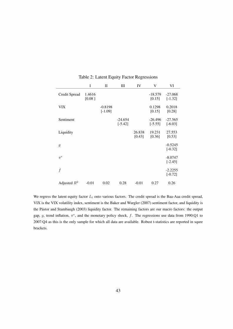
Table 2: Latent Equity Factor Regressions

I II III IV V VI

Credit Spread 1.4616 -18.579 -27.068[0.08 ] [0.15] [-1.32]

VIX -0.8198 0.1298 0.2018[-1.09] [0.15] [0.28]

Sentiment -24.654 -26.496 -27.565[-5.42] [-5.55] [-6.03]

Liquidity 26.838 19.231 27.553[0.43] [0.36] [0.53]

g -0.5245[-0.32]

πe -8.0747[-2.45]

f -2.2255[-0.72]

Adjusted R2 -0.01 0.02 0.28 -0.01 0.27 0.26

We regress the latent equity factor Lt onto various factors. The credit spread is the Baa-Aaa credit spread,

VIX is the VIX volatility index, sentiment is the Baker and Wurgler (2007) sentiment factor, and liquidity is

the Pastor and Stambaugh (2003) liquidity factor. The remaining factors are our macro factors: the output

gap, g, trend inflation, πe, and the monetary policy shock, f . The regressions use data from 1990:Q1 to

2007:Q4 as this is the only sample for which all data are available. Robust t-statistics are reported in squre

brackets.

43

Table 3: Decomposing Total Expected Equity Returns

(1) (2) (3) (4) (5) (6) (7)

Real Inflation Cashflow Real ExpectedDuration Expected Risk Risk Risk Total

Real rate Premium Inflation Premium Premium Premium Return

k (yrs) r DP E(π) IRP CFP RRP E(RE,$)

Panel A: Mean Decomposition

5 2.9756 0.0604 3.0950 0.4142 4.7139 5.1281 11.25910 2.9756 0.5020 3.0028 0.6048 3.8409 4.4457 10.92615 2.9756 0.8012 2.9460 0.6241 3.7018 4.3259 11.049

Panel B: Variance Decomposition

5 0.1888 0.0810 0.0043 0.0036 0.7223 0.7259 1.000010 0.3745 0.1781 0.0030 0.0112 0.4332 0.4444 1.000015 0.4376 0.2229 0.0020 0.0133 0.3242 0.3375 1.0000

We report decompositions of the expected total equity return, Et(RE,$t (k)), in Panel A and its variance

in Panel B into various risk premiums; real short rate, rt; real duration premium, DPt(k); inflation risk

premium, IRPt(k); expected inflation, Et(πt(k)); real risk premium, RRPt(k), and the real cashflow risk

premium, CFPt(k), as defined in Section 2.7. The total expected return in (7) is the sum of columns (1) to

(5). The real risk premium is the sum of columns (4) and (5). Horizons k are given in years. The numbers

in the mean decomposition are in annualized percentage terms. The premiums are computed at the sample

mean of the factors.

44

Tabl

e4:

Cor

rela

tions

ofM

acro

and

Ris

kPr

emiu

ms

rr$

gπe

fd

L

Rea

lDur

atio

nPr

emiu

m,D

P-0

.901

4-0

.717

9-0

.459

50.

0568

-1.0

000

0.04

15-0

.250

4

Infla

tion

Ris

kPr

emiu

m,I

RP

0.79

440.

9350

1.00

000.

1964

-0.4

595

-0.1

544

0.12

13

Cas

hflow

Ris

kPr

emiu

m,C

FP

0.00

310.

0141

0.19

641.

0000

0.05

680.

0701

0.57

82

Rea

lRis

kPr

emiu

m,R

RP

0.12

530.

1575

0.34

220.

9885

-0.0

164

0.04

340.

5727

Exp

ecte

dE

quity

Ret

urn,E[R

E,$(k)]

0.41

980.

5151

0.69

130.

8428

-0.1

824

-0.0

298

0.50

82

We

repo

rtco

rrel

atio

nsof

the

real

shor

trat

ean

dva

riou

sri

skpr

emiu

ms

and

spre

ads,

asde

fined

inSe

ctio

n2.

7.T

heva

riab

ler

deno

tes

the

real

shor

t

rate

,r$

isth

e(n

omin

al)F

edFu

nds

rate

,gth

eou

tput

gap,

πe

istr

end

infla

tion,

fis

am

onet

ary

polic

ysh

ock,

dis

real

divi

dend

grow

th,a

ndL

is

the

late

nteq

uity

prem

ium

fact

or.T

heho

rizo

nisk=

10ye

ars,

exce

ptfo

rthe

shor

trat

ean

dth

edi

vide

ndyi

eld.

45

Table 5: Factor Variance Decompositions of Risk Premiums

g πe f d L

Real Short Rate, r 0.0294 0.3774 0.5932 0.0000 0.0000

Real Duration Premium, DP 0.0062 0.0473 0.9465 0.0000 0.0000

Expected Inflation, E[π(k)] 0.1160 0.8840 0.0000 0.0000 0.0000

Inflation Risk Premium, IRP 0.0125 0.9211 0.0664 0.0000 0.0000

Cashflow Risk Premium, CFP 0.6186 0.0174 0.0415 0.0000 0.3225

Real Risk Premium, RRP 0.6015 0.0429 0.0422 0.0000 0.3134

Expected Equity Return, E[RE , $(k)] 0.2703 0.5007 0.0018 0.0000 0.2272

We report decompositions of the variance of the real short rate and various risk premiums, as defined in

Section 2.7. The variable g denotes the output gap, πe is trend inflation, f is a monetary policy shock, d is

real dividend growth, and L is the latent equity premium factor. The horizon is k = 10 years for all risk

premiums and expected inflation, except for the real short rate.

46

Figure 1: Output Gap, Trend Inflation, and Monetary Policy Shocks

1985 1990 1995 2000 2005−8

−6

−4

−2

0

2

4

6

8fg

πe

We plot the output gap, gt, trend inflation, πet , and the monetary policy shock, ft. All variables have been

demeaned and are annualized. Shaded areas represent NBER recessions. The sample is from 1982:Q1 to

2008:Q4 and the frequency is quarterly.

47

Figure 2: Real and Nominal Short Rates

1985 1990 1995 2000 2005−2

0

2

4

6

8

10

12

14r

r$

We plot the real short rate, r, which is implied by the model in equation (12) and unobserved in data, and the

nominal short rate, r$, which is the Fed Funds rate. Shaded areas represent NBER recessions. The sample is

from 1982:Q1 to 2008:Q4 and the frequency is quarterly.

48

Figure 3: Nominal Yield Curve

10 20 30 40 50 604

4.5

5

5.5

6

6.5

7

7.5

8

datamodel

We plot the model-implied average term structure of nominal zero-coupon bonds (solid line) together with

average yields, with two standard error bounds, in data. Maturities on the x-axis are in quarters and the yields

are annualized on the y-axis. The sample is from 1982:Q1 to 2008:Q4.

49

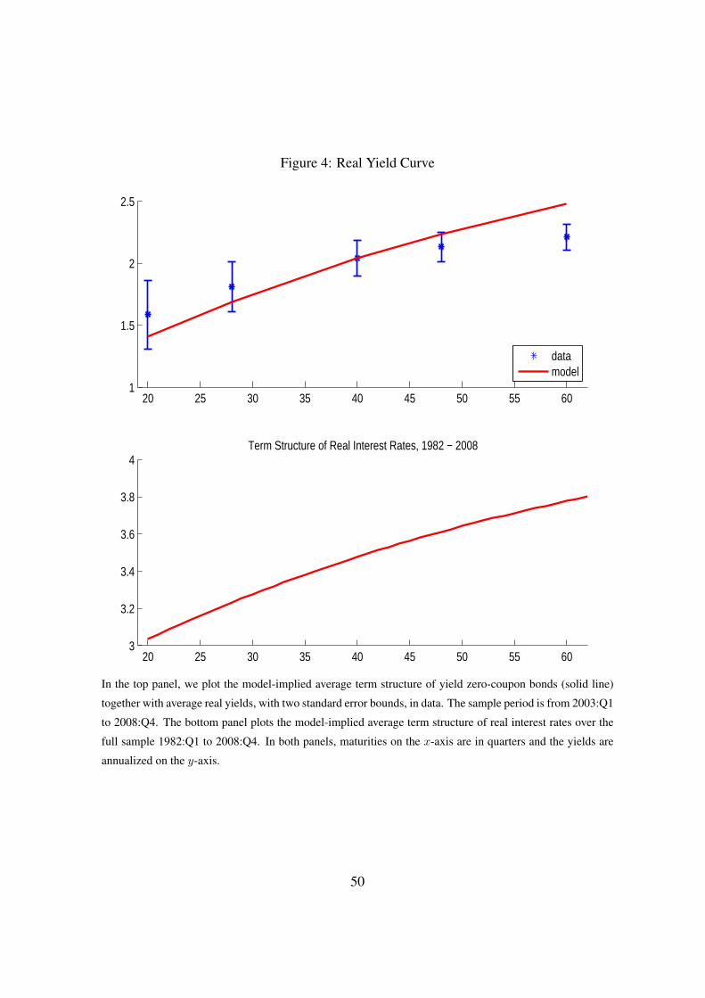
Figure 4: Real Yield Curve

20 25 30 35 40 45 50 55 601

1.5

2

2.5

datamodel

20 25 30 35 40 45 50 55 603

3.2

3.4

3.6

3.8

4Term Structure of Real Interest Rates, 1982 − 2008

In the top panel, we plot the model-implied average term structure of yield zero-coupon bonds (solid line)

together with average real yields, with two standard error bounds, in data. The sample period is from 2003:Q1

to 2008:Q4. The bottom panel plots the model-implied average term structure of real interest rates over the

full sample 1982:Q1 to 2008:Q4. In both panels, maturities on the x-axis are in quarters and the yields are

annualized on the y-axis.

50

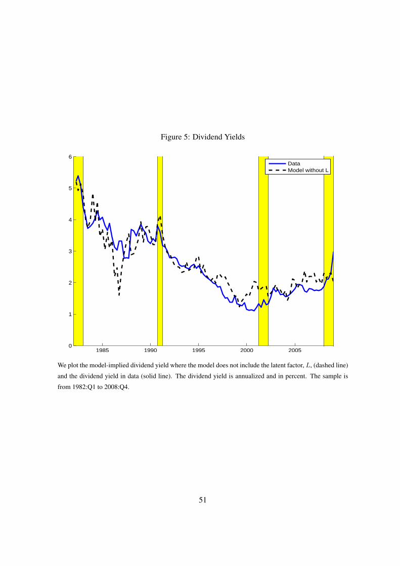
Figure 5: Dividend Yields

1985 1990 1995 2000 20050

1

2

3

4

5

6DataModel without L

We plot the model-implied dividend yield where the model does not include the latent factor, L, (dashed line)

and the dividend yield in data (solid line). The dividend yield is annualized and in percent. The sample is

from 1982:Q1 to 2008:Q4.

51

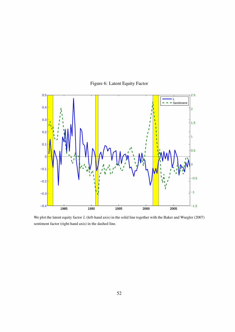
Figure 6: Latent Equity Factor

1985 1990 1995 2000 2005−0.4

−0.3

−0.2

−0.1

0

0.1

0.2

0.3

0.4

0.5

1985 1990 1995 2000 2005−1.5

−1

−0.5

0

0.5

1

1.5

2

2.5LSentiment

We plot the latent equity factor L (left-hand axis) in the solid line together with the Baker and Wurgler (2007)

sentiment factor (right-hand axis) in the dashed line.

52

Figure 7: Term Structure of Equity Returns

5 10 15 20 25 30 35 40 45 50 55 600

2

4

6

8

10

12

14

16

18

20

CFPRRP

Et[RE,$

t]

We plot the term structure of the total equity return, Et[RE,$t (k)], in the solid line, the cashflow premium,

CFPt(k), defined in equation (31) in the dashed line, and the real equity risk premium, RRPt(k) defined in

equation (32) in the dashed-dotted line for various k starting at the sample mean of the factors. Maturities on

the x-axis are in quarters.

53

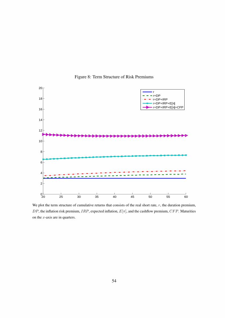
Figure 8: Term Structure of Risk Premiums

20 25 30 35 40 45 50 55 600

2

4

6

8

10

12

14

16

18

20

rr+DPr+DP+IRPr+DP+IRP+E[π]r+DP+IRP+E[π]+CFP

We plot the term structure of cumulative returns that consists of the real short rate, r, the duration premium,

DP , the inflation risk premium, IRP , expected inflation, E[π], and the cashflow premium, CFP . Maturities

on the x-axis are in quarters.

54

Figure 9: Risk Premiums

Panel A: Expected Total Equity Return

1985 1990 1995 2000 2005−10

0

10

20

30

40

1985 1990 1995 2000 20050

2.5

5

7.5

10

E[RE,$t

]

Dividend Yield

Panel B: Risk Premiums

1985 1990 1995 2000 2005

−8

−6

−4

−2

0

2

4

6

8Duration Premium

1985 1990 1995 2000 2005−2

−1

0

1

2

3

4

5Inflation Compensation

IRPE[π]

1985 1990 1995 2000 2005

0

5

10

15Real Short Rate

1985 1990 1995 2000 2005−10

−5

0

5

10

15

20Cashflow and Real Risk Premiums

CFPRRP

55

Note to Figure 9In Panel A, we plot the total expected nominal equity return for a 10-year horizon, Et[R

E,$t (k)] for k = 40

quarters, implied by the model in the solid line. Units on the left-hand y-axis are in percent and correspond

to the expected equity return. We overlay the dividend yield, which is plotted in the dotted line and has

units on the right-hand y-axis in percent. In Panel B, we decompose the total expected equity return into the

real short rate, real duration premium, expected inflation (E(π)) and the inflation risk premium (IRP), and

the cashflow risk premium (CFP) and the real risk premium (RRP). All of these components correspond to

a 10-year horizon and are defined in Section 2.7. Shaded areas represent NBER recessions. The sample is

from 1982:Q1 to 2008:Q4 and the frequency is quarterly.

56

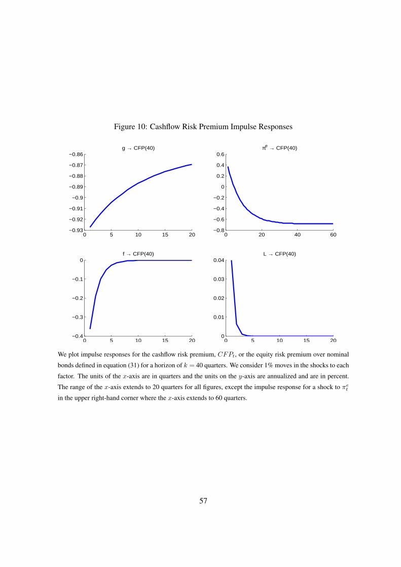
Figure 10: Cashflow Risk Premium Impulse Responses

0 5 10 15 20−0.93

−0.92

−0.91

−0.9

−0.89

−0.88

−0.87

−0.86g → CFP(40)

0 20 40 60−0.8

−0.6

−0.4

−0.2

0

0.2

0.4

0.6πe → CFP(40)

0 5 10 15 20−0.4

−0.3

−0.2

−0.1

0f → CFP(40)

0 5 10 15 200

0.01

0.02

0.03

0.04L → CFP(40)

We plot impulse responses for the cashflow risk premium, CFPt, or the equity risk premium over nominal

bonds defined in equation (31) for a horizon of k = 40 quarters. We consider 1% moves in the shocks to each

factor. The units of the x-axis are in quarters and the units on the y-axis are annualized and are in percent.

The range of the x-axis extends to 20 quarters for all figures, except the impulse response for a shock to πet

in the upper right-hand corner where the x-axis extends to 60 quarters.

57

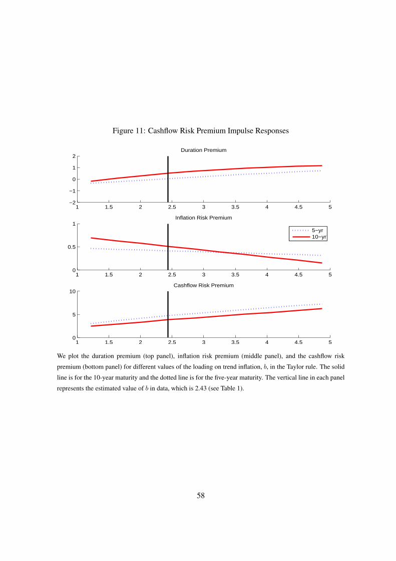
Figure 11: Cashflow Risk Premium Impulse Responses

1 1.5 2 2.5 3 3.5 4 4.5 5−2

−1

0

1

2Duration Premium

1 1.5 2 2.5 3 3.5 4 4.5 50

0.5

1Inflation Risk Premium

5−yr10−yr

1 1.5 2 2.5 3 3.5 4 4.5 50

5

10Cashflow Risk Premium

We plot the duration premium (top panel), inflation risk premium (middle panel), and the cashflow risk

premium (bottom panel) for different values of the loading on trend inflation, b, in the Taylor rule. The solid

line is for the 10-year maturity and the dotted line is for the five-year maturity. The vertical line in each panel

represents the estimated value of b in data, which is 2.43 (see Table 1).

58