This is a repository copy of Nominal and local stress quantities to design aluminium-to-steel thin welded joints against fatigue.

White Rose Research Online URL for this paper:https://eprints.whiterose.ac.uk/142479/

Version: Accepted Version

Article:

Al Zamzami, I., Davison, J. and Susmel, L. orcid.org/0000-0001-7753-9176 (2019) Nominal and local stress quantities to design aluminium-to-steel thin welded joints against fatigue. International Journal of Fatigue, 123. pp. 279-295. ISSN 0142-1123

https://doi.org/10.1016/j.ijfatigue.2019.02.018

Article available under the terms of the CC-BY-NC-ND licence (https://creativecommons.org/licenses/by-nc-nd/4.0/).

eprints@whiterose.ac.ukhttps://eprints.whiterose.ac.uk/

Reuse

This article is distributed under the terms of the Creative Commons Attribution-NonCommercial-NoDerivs (CC BY-NC-ND) licence. This licence only allows you to download this work and share it with others as long as you credit the authors, but you can’t change the article in any way or use it commercially. More information and the full terms of the licence here: https://creativecommons.org/licenses/

Takedown

If you consider content in White Rose Research Online to be in breach of UK law, please notify us by emailing eprints@whiterose.ac.uk including the URL of the record and the reason for the withdrawal request.

1

Nominal and local stress quantities to design

aluminium-to-steel thin welded joints against fatigue

Ibrahim Al Zamzami, Buick Davison and Luca Susmel

Department of Civil and Structural Engineering, The University of Sheffield,

Mappin Street, Sheffield S1 3JD, United Kingdom

Corresponding Author: Prof. Luca Susmel

Department of Civil and Structural Engineering

The University of Sheffield, Mappin Street, Sheffield, S1 3JD, UK

Telephone: +44 (0) 114 222 5073

Fax: +44 (0) 114 222 5700

E-mail: l.susmel@sheffield.ac.uk

ABSTRACT

Welding aluminium to steel to make mechanical joints is possible, but there is, to date, no

accepted method for performing the fatigue assessment of such hybrid connections. In this

context, the present investigation aims at checking the accuracy of nominal stresses, effective

notch stresses, notch-stress intensity factors, and the Modified Wöhler Curve method (applied

in conjunction with the Theory of Critical Distances) in estimating fatigue lifetime of butt,

cruciform, lap and tee aluminium-to-steel thin welded joints. EWM coldArc® welding

technology was used to manufacture the welded specimens that were used for this validation

exercise. The samples being tested in the structural laboratory of the University of Sheffield,

UK, were manufactured by using AA1050 aluminium and EN10130:1991 steel with main plates

thicknesses of 1 mm or 2 mm. The results from this experimental/theoretical investigation

demonstrate that all the design methodologies being investigated can be used to perform the

fatigue assessment of aluminium-to-steel thin welded joints provided that suitable

reference/calibration fatigue curves are used. In the present paper, some quantitative

recommendations are given for use in situations of practical interest of the design techniques

being considered.

Keywords: aluminium-to-steel welds, nominal stress, local stress, critical plane, critical

distance.

2

Nomenclature

a, b, α, β fatigue constants for the MWCM’s calibration curves

c0, c1 constants in the linear regression function

k negative inverse slope k0 negative inverse slope of the torsional fatigue curve kτ negative inverse slope of the modified Wöhler curve

KI, KII notch-stress intensity factor (N-SIF) for Mode I and Mode II loading

NA reference number of cycles to failure NRef reference number of cycles to failure

Nf number of cycles to failure

PS probability of survival

q factor for one-sided tolerance limits for normal distribution

r, polar coordinates

rn notch root radius

rref reference radius rreal actual root radius in welded joints

R load ratio (R=min/max)

t thickness

T scatter ratio of the endurance limit range for PS=90% and PS=10%

z weld leg length

max, min maximum and minimum stress in the cycle

, r linear-elastic local normal stresses ρw critical plane stress ratio

1, 2, 1, 2 constants in William’s equations

KI mode I N-SIF range

KI,50% mode I N-SIF range extrapolated at NA cycles to failure for PS=50%

KI,97.7% mode I N-SIF range extrapolated at NA cycles to failure for PS=97.7%

stress range

1 range of the maximum principal stress

A,50% endurance limit range at NA cycles to failure for PS=50%

A,97.7% endurance limit range at NA cycles to failure for PS=97.7%

nom nominal stress range

NS notch stress range ∆τRef reference shear stress range extrapolated at 𝑁𝑅𝑒𝑓 cycles to failure

3

1. Introduction

For more than a century, engineers have been developing welding technologies in a systematic

way as an economical and versatile joining process to replace, where appropriate, the use of

mechanical fasteners [1]. Avoidance of fatigue failure associated with the welding process was

identified as important from the outset, so that a considerable amount of literature has been

published on the effect of the welding process on the durability of weldments subject to fatigue

loading. By comparing the robustness of welded and un-welded components made from the

same material, a significant reduction in the fatigue strength of welded components is

observed [2-4]. This strength reduction is caused by the introduction during welding of

residual stresses, imperfections and distortions. Further, localised stress concentrations are

common and result in severe stress/strain gradients at the weld toes/roots causing fatigue

cracks to initiate in the vicinity of these critical regions [5].

There is a large volume of published studies describing the fatigue behaviour of welded

structural details made of either steel or aluminium. These studies consider different fatigue

design approaches to estimate the fatigue lifetime of structural components. The available

Standards and Codes of Practice [6, 7, 8] suggest different design methods including those

based on the use of nominal stress as well as of effective notch stresses. The nominal stress

approach, which is undoubtedly the simplest and most widely used design methodology,

estimates fatigue strength by simply selecting an appropriate S-N curve amongst those

provided by the Standard Codes for each specific welded detail [9]. However, the nominal

stress approach is limited to designing only those specific welded geometries for which a

reference S-N curve is available.

A more advanced method recommended by the International Institute of Welding (IIW) [6] is

the so-called effective notch stress approach. This method estimates the fatigue strength of

welded connections by assuming that weld toes/roots behave like rounded notches with a

radius equal to 1 mm for a plate thickness larger than or equal to 5 mm [6] and to 0.05 mm for

a main plate thickness lower than 5 mm [10-15].

Another method that can be successfully used to assess the fatigue strength of welded joints is

the so-called Notch-Stress Intensity Factor (N-SIF) approach [16, 17]; this fatigue assessment

technique is based on William’s solutions [18] for V-notches having a tip radius equal to zero.

Recently, attention has been focused on extending the use of the Theory of Critical Distances

(TCD) to the fatigue assessment of welded joints [19, 20]. The TCD groups together a number

of local stress-based approaches where fatigue damage in the presence of any kind of stress

concentrator is estimated by directly post-processing the linear-elastic stress fields acting on

the materials in the vicinity of the assumed crack initiation locations. The TCD provides very

accurate estimations of the fatigue lifetime of welded components and requires less

computational effort than the effective notch stress approach [19, 21].

4

As reducing the overall weight of vehicles leads to a reduction in fuel consumption [22],

current developments in the transportation industry have sought to replace the ferrous

metallic components with lightweight structural metals such as aluminium alloys. As a result,

significant attention has been paid in recent years to develop welding technologies capable of

joining aluminium to steel metallurgically to achieve not only strong hybrid joints, but also

higher productivity [23-26]. Because aluminium alloys and steel have incompatible thermal

and physical properties and also different metallurgical characteristics, conventional fusion

welding becomes problematic. During welding the formation of intermetallic phases (Fe-Al)

deteriorates the strength of the joints by introducing brittle layers at the interface between the

two materials [27-32]. To overcome this problem, in recent years different welding techniques

have been developed and optimised, with welding technology coldArc® commercialised by

EWM (www.ewm-group.com) being, to date, the most advanced solution which provides

excellent arc-stability and highly controlled heat input [33, 34].

Understanding of the fatigue behaviour of welded joints made using dissimilar materials (and,

in particular, aluminium alloys and steel) is very limited. Before investigating the fatigue

behaviour of aluminium-to-steel welded joints, it is important to understand the static

behaviour of such connections. A recent experimental study [35] was carried out in order to

investigate the static behaviour of aluminium-to-steel thin welded joints with different

geometrical configurations - including butt-welded joints (with weld seam inclination angles

ranging between 0º and 60º), cruciform connections, and lap joints. This study highlighted

that, regardless of the joint configuration or the angle of inclination, the fracture of these

hybrid connections always took place in the aluminium heat affected zone. This experimental

finding confirmed that Eurocode 9 [36] can be used to design aluminium-to-steel welded

joints with a high level of accuracy [35].

The present paper reports the findings of an experimental, theoretical, and numerical study

on the fatigue behaviour of aluminium-to-steel thin welded joints under uniaxial cyclic

loading. The ultimate aim of the present investigation is to recommend appropriate design

strategies suitable for accurately performing the fatigue assessment of aluminium-to-steel

hybrid welded connections.

2. Experimental Procedure

An experimental investigation was designed to generate a large number of data suitable for

checking the accuracy and reliability of different design approaches in estimating fatigue

strength of steel-to-aluminium thin welded joints. The details of this extensive experimental

work are summarised in the following sub-sections.

5

2.1 Materials

The materials used in this investigation were aluminium alloy AA1050 (containing 99.5% of

aluminium) and a zinc-coated cold-rolled low carbon steel manufactured in accordance with

EN 10130:1991. The ultimate tensile strength of these two materials were 120 MPa and 410

MPa, respectively, with Young’s modulus equal to 71 GPa for the aluminium alloy and to 210

GPa for the steel. The thickness of the zinc coating on the steel sheets was measured to be 25

μm.

The 1 mm diameter filler wire used in the welding process was made of AA4043 aluminium

alloy. During welding, pure argon was used as shielding gas. Two different sheet thicknesses

(i.e., 1 mm and 2 mm) were used to manufacture the fatigue specimens to be tested under load

ratios, R, equal to -1, 0.1, and 0.5. The chemical compositions of the materials used in this

investigation are summarised in Table 1.

2.2 Welding of the fatigue specimens

Various welded joint configurations (see Fig. 1) were manufactured by an experienced

technician using an EWM alpha Q551 pulse machine. Welding technology EWM coldArc® is a

modified short-arc process that has gap bridge capabilities and can provide effective control

over the heat input and the metal transfer. As far as very thin materials are concerned, the low

heat input allows them to be welded together without causing burn-through. The coldArc®

process is able to joint hybrid sheets with a thickness as thin as 0.3 mm and 0.7 mm using

automated and manual welding machines, respectively. The unique features of the coldArc®

technology make it suitable for fabricating aluminium-to-steel thin joints, provided that the

steel sheet is pre-coated with zinc to prevent the formation of hard and brittle intermetallic

phases at the interface between the two materials.

EWM provides very detailed welding parameter envelopes for different welding combinations

and different thicknesses. For the 1 mm thick sheets, the welding parameters were set as

follows: arc voltage equal to 15.3 V, current to 54 A, wire feed to 5 m/min; for the 2 mm thick

plates the parameters were: arc voltage equal to 18.2 V, current to 88 A, wire feed to 7.9

m/min. The specimens were manufactured by welding aluminium and steel sheets having

width equal to 70 mm. The welded samples were subsequently cut down to 50 mm width to

eliminate any undesirable defects formed at the edges during the welding process.

2.3 Investigated welded geometries

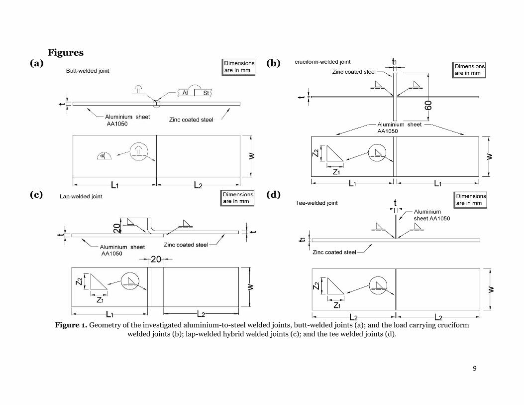
Four different geometrical configurations were manufactured and prepared for fatigue testing,

including butt, cruciform, lap and tee-welded joints (Fig. 1).

The butt joints were fabricated by using a single weld (Fig. 1a). It is important to point out here

that the galvanised steel sheets were zinc-coated solely on the top and bottom surfaces, leaving

6

the edges with no zinc. Thus, the butt-welded joints were characterised by a lack of adhesion

between the steel and the aluminium. This lack of adhesion resulted in a gap between the two

materials, so that the overall mechanical strength was due to the weld that acted as a bridge

holding the two materials together (see Fig. 1a).

The manufacturing of the cruciform welded joints was performed using a welding jig

specifically designed to ensure that the top and bottom stiffeners were aligned and welded as

straight as possible (Fig. 1b). This effectively minimised any detrimental phenomena

associated with eccentricity.

Because the steel edges were not galvanised, producing the lap joint in the traditional form

was not possible. Accordingly, the lap joints being tested were manufactured by bending the

steel sheet at 90º. As can be seen in Fig. 1c, this allowed the weld seam to be placed between

the galvanised steel and the aluminium. As will be discussed below in detail, due to the specific

geometrical features characterising these welded specimens, this particular shape was taken

into account explicitly when determining the local stress fields being used to assess fatigue

strength.

Finally, the tee-welded joints were prepared with the stiffener made of aluminium and the

main plate made of steel (Fig. 1d). To prevent the main plate from bending during welding, all

the tee-welded joints were manufactured by using sheets having thickness equal to 2 mm.

2.4 Fatigue testing

The fatigue tests were run at room temperature by using a 100 kN capacity MAYSE dynamic

machine. The specimens were tested in the as-welded condition under a frequency of 10 Hz.

Prior to fatigue testing, the clear distance between the weld seam regions and the hydraulic

grips was set to approximately 20 mm for all the welded configurations. This allowed us to

minimise any secondary bending effect. As to this aspect, it is important to highlight that no

external fixtures were used to support the specimens during testing. This is because all the

specific supporting devices being available in our testing laboratory were seen to somehow

affect the way the loading was applied to the thin welded joints. Accordingly, in order to

generate sets of valid fatigue results, the different welded geometries were tested as detailed

in what follows.

For the butt and cruciform welded joints, two different plate thicknesses were used: 1 mm for

a load ratio equal to 0.1, and 2 mm for a load ratio equal to -1. Under fully-reversed loading

(i.e., R=min/max=-1), the 2 mm thickness plates provided sufficient stiffness to prevent, under

the compressive part of the cyclic loading, secondary bending from affecting the fatigue results

being generated.

In contrast, since the lap joints were rather long, the excessive deflection due to secondary

bending made it impossible for this specific welded geometry to be tested under fully-reversed

7

axial loading. Accordingly, the lap joints with thickness equal to 1 mm were tested under

R=0.1, whereas those with thickness equal to 2mm under R=0.5.

Finally, the tee-welded joints with thickness equal to 2 mm were tested by setting the load

ratio equal to -1 as well as to 0.1.

3. Lifetime estimation using the nominal stress approach

The nominal stress-based approach is one of the most widely used methods that is employed

in situations of practical interest to perform the fatigue assessment of welded components.

This approach postulates that the required design stresses have to be calculated according to

classic continuum mechanics by directly referring to the nominal cross-sectional area.

Nominal stresses are determined without taking into account localised stress raising

phenomena due to the presence of the weld toe as these phenomena are already included in

the reference fatigue design curves being provided by the available design codes - such as

Eurocode 9 (EC9) [7], Eurocode 3 (EC3) [8], and the IIW Recommendations [6].

Consequently, the selection of an appropriate design curve is essential to ensure that accurate

fatigue design is achieved [6, 37-40]. Although the nominal stress approach is simple and

accurate, unfortunately, it cannot be used to design complex/non-standard welded details [37]

unless the specific design curve being needed is generated by running appropriate

experiments.

Turning to aluminium-to-steel welded joints, currently, there is no guidance for the static and

fatigue assessment of these hybrid welded connections. As far as static failures are concerned,

examination of the state of the art demonstrates that, so far, the international scientific

community has focused its attention mainly on studying the existing interactions amongst

welding technologies, material microstructural features and ultimate tensile strength [24, 34,

35, 41-46]. In this context, in a recent investigation [35] it was observed that static fracture of

aluminium-to-steel welded joints always occurs in the heat affected zone on the aluminium

side. In contrast, the direct inspection of the fracture surfaces generated under fatigue loading

revealed that the fatigue breakage of aluminium-to-steel welded joints always took place at the

interface between weld toe and aluminium plate (Fig. 2). This strongly supports the idea that

in aluminium-to-steel welded connections the crack initiation process was favoured by

localised stress concentration phenomena occurring in the weld seam region.

Based on the above experimental evidence, the hypothesis was formed that aluminium-to-

steel welded joints behave like conventional welded connections so that, in situations of

practical interest, they can be designed against fatigue by directly using the nominal stress

approach along with the design curves recommended by EC9 [7], EC3 [8] and the IIW [6].

The results of the re-analyses performed in terms of nominal stresses are summarised in

Tables 2 to 5. These tables were populated by post-processing the experimental results,

8

expressed in terms of nominal stress ranges, under the hypothesis of a log-normal distribution

of the number of cycles to failure for each stress level, with the confidence level being set equal

to 95% [39]. The ranges of the endurance limits listed in Table 6 were extrapolated at 2∙106

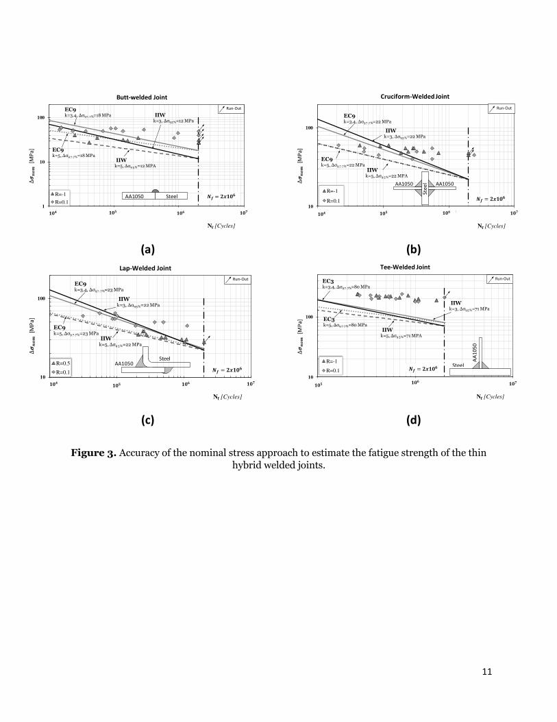
cycles to failure for a probability of survival, 𝑃𝑠, equal to 50% and 97.7%. Figure 3 presents the

same results in log-log Wöhler diagrams, where, for the different welded configurations being

investigated, the nominal stress range, ∆𝜎𝑛𝑜𝑚, is plotted against the number of cycles to failure, 𝑁𝑓. In addition, the design curves recommended by EC9 [7], EC3 [8] and the IIW [9] for each

welded geometry are also plotted in the charts of Fig. 3, which allows the experimental results

to be compared directly with the standard design curves.

Table 6 and the Wöhler diagrams of Figs 3a to 3c make it evident that the values of the negative

inverse slope, k, determined for the investigated welded configurations were much larger not

only than the value of 3 recommended by the IIW [9], but also than the value of 3.4 suggested

by EC9 [7]. This is not surprising since the negative inverse slopes provided by the available

design codes were determined by re-analysing a large number of experimental results

generated by testing welded joints that were thick and stiff - i.e., welded connections with

thickness much larger than 5 mm. In contrast, the experimental fatigue curves experimentally

determined by testing thin and flexible welded connections are seen to be characterised by a

negative inverse slope that varies in the range 3-6 [47]. This is the reason why Sonsino et al.

[47] recommend performing the fatigue assessment of thin welded joints via fatigue curves

that have the same endurance limit (at 2 million cycles) as the one provided by the pertinent

standard codes and negative inverse slope invariably equal to 5.

By applying the strategy recommended by Sonsino and co-workers to assess the fatigue

strength of thin welded joints [47], the use of the modified EC9 design curves (grey dotted line

in Figs 3a to 3c) and the modified IIW design curves (black dashed line in Figs 3a to 3c) lead

to a more conservative estimation of the fatigue lifetime of aluminium-to-steel welded joints.

In particular, as per the Wöhler diagrams of Figs 3a to 3c, the modified IIW design curves were

seen to provide conservative fatigue lifetime estimations for all the welded configurations. In

contrast, the modified EC9 curves were seen to result in conservative fatigue strength

predictions in all cases except for butt joints (Fig. 3a).

Turning to the non-load carrying fillet tee-welded joints (Fig. 3d), the steel plates were

subjected to fatigue loading whereas the aluminium plates acted solely as stiffeners. Although

the tee-welded joints were 2 mm thick (i.e., thin joints), the negative inverse slope was kept

the same as suggested by the design codes for plates with thickness larger than 5 mm, with

this still resulting in conservative estimations. This means that the use of a k value equal to 5

as suggested by Sonsino et al. for thin plates [47] resulted in an even higher level of

conservatism in estimating the fatigue lifetime of the tee-welded joint (Fig. 3d).

9

To summarise, using the nominal stress approach, the fatigue behaviour of aluminium-to-

steel butt (Fig. 3a), cruciform (Fig. 3b), and lap (Fig. 3c) welded joints can be assessed by

treating the joints as conventional aluminium-to-aluminium welded joints, with a higher

degree of accuracy being reached by setting, as suggested by Sonsino et al. [47], the negative

inverse slope equal to 5. In contrast, as far as hybrid tee-welded joints are concerned (Fig. 1d),

these connections can be treated as standard steel-to-steel joints and designed by following

either the IIW recommendations or EC3, with this being done without the need for adjusting

the value of the negative inverse slope.

4. Lifetime estimation in terms of effective notch stresses

The effective notch stress approach is a well-known methodology that is widely used in

industry to determine the fatigue strength of welded details. This approach is also the most

advanced design methodology recommended by the IIW. This method estimates fatigue

strength by using linear-elastic notch stresses calculated by fictitiously rounding the weld toes

or the weld roots [9, 12, 48]. By taking full advantage of the micro-support theory formulated

by Neuber to model sharp cracks, Radaj [49-53] developed the effective notch stress approach

by proposing to use a fictitious radius, rref, equal to 1 mm, with this value for rref being

recommended to be adopted solely to assess welded connections with thickness larger than 5

mm (see Fig. 4a). In contrast, for welded details with thickness lower than 5 mm, weld

toes/roots should be rounded by adopting a fictitious radius equal to 0.05 mm [13, 49, 54-57].

As far as aluminium welded joints with thickness larger than 5 mm are concerned, the IIW [6]

recommends to assess their fatigue strength by using a design curve having notch stress

endurance limit range, ∆σA,97.7, equal to 71 MPa (extrapolated at 2.106 cycles to failure for a

probability of survival, Ps, equal 97.7%) and negative inverse slope, k, equal to 3. In contrast,

an aluminium welded detail with thickness lower than 5 mm should be designed against

fatigue by using the FAT180 design curve, i.e., a fatigue curve having k equal to 5 and ∆𝜎𝐴,97.7

equal to 180 MPa (with this endurance limit being again determined at 2.106 cycles to failure

for a Ps equal 97.7%) [12, 47].

In order to post-process the experimental data according to the effective notch stress

approach, the stress analysis was carried out by using FE code ANSYS® to solve linear-elastic

bi-dimensional models (Fig. 5a). Since the welded joints being investigated had thickness

lower than 5 mm, design notch stresses were calculated by rounding the weld toes of the lap

and cruciform joints and the roots of the butt joints by setting the reference radius, rref , equal

to 0.05 mm. The mesh density in the vicinity of the fictitious fillet radii was gradually refined

until convergence occurred.

The experimental results post-processed according to the effective notch stress approach, for

the butt (Fig.1a), cruciform (Fig.1b) and lap welded joints (Fig.1c) are listed in Table 2-4. The

10

same results are also plotted in the log-log Wöhler diagrams of Figs 4c, 4d and 4e. Table 6

summarises the results from the statistical reanalysis in terms of negative inverse slope and

endurance limit range, ∆σA, extrapolated at 2∙106 cycles to failure for a probability of

survival, Ps, equal to 50% and to 97.7%.

Turning back to the stress analysis aspects, as far as the tee-welded joints were concerned, the

maximum stress was seen to occur at the interface between the aluminium weld and the steel

plate rather than at the weld toe (Fig.4b). Accordingly, since for this specific configuration the

notch stress approach could not be applied rigorously, the tee-welded joints (Fig.1d) were then

excluded from the present re-analysis.

The S-N charts of Figs 4c to 4e demonstrate that the use of the FAT180 curve recommended

by Sonsino et al. to design aluminium-to-aluminium welded joints [12, 47] was not capable of

satisfactorily modelling the fatigue behaviour of the hybrid welded specimens being tested,

with its use resulting in a large degree of non-conservatism.

In order to determine a fatigue curve suitable for designing aluminium-to-steel welded joints

according to the notch stress approach, all the data generated were then re-analysed together.

By so doing, as per the Wöhler diagram of Fig. 4f, the most appropriate design curve to be used

to model the fatigue strength of our aluminium-to-steel thin welded specimens was seen to be

the one having endurance fatigue limit range equal to 90 MPa (at 2∙106 cycles to failure for Ps

equal to 97.7%) and inverse negative slope equal to 5.

To conclude, a recommended value for the endurance limit of 90 MPa was derived in

accordance with the IIW numeric system [6], whereas the value for the negative slope was

chosen according to the value that is recommended by Sonsino et al. to design thin and flexible

welded joints [47].

5. Lifetime estimation in terms of the N-SIFs approach

By taking full advantage of the classic analytical solution devised by Williams [18], Verreman

and Nie [58] laid the foundations of the Notch-Stress Intensity Factor (N-SIF) approach [59,

60]. In order to understand the fundamental idea on which the N-SIF approach is based,

consider the joint sketched in Fig. 6a. In this connection the toe radius, 𝑟𝑛, of the weld seam is

assumed to be invariably equal zero. According to the system of coordinates as defined in Fig.

6a, the linear elastic stress field in the vicinity of the weld seam can be described analytically

via the following relationships for Mode I and Mode II loading, respectively [61, 62]:

{ σθσrτrθ} = 1√2π rλi−1KI(1 + λi) + χi(1 − λi) [{(1 + λi)cos (1 − λi)θ(3 − λi)cos (1 − λi)θ(1 − λi)sin (1 − λi)θ} + χi { cos (1 + λi)θ−cos (1 + λi)θsin (1 + λi)θ }] (1)

11

{ σθσrτrθ} = 1√2π rλi−1KII(1 + λi) + χi(1 − λi) [{(1 + λi)cos (1 − λi)θ(3 − λi)cos (1 − λi)θ(1 − λi)sin (1 − λi)θ} + χi { cos (1 + λi)θ−cos (1 + λi)θsin (1 + λi)θ }] (2)

In Eqs (1) and (2) λi and χi (i=1, 2) are parameters depending on the opening angle of the V-

notch [64]. KI and KII are instead the N-SIFs for Mode I and Mode II loading, respectively, and

can be determined according to the following definitions [62, 63]:

KI = √2π limr→0(σθ)θ=0r1−λ1 (3) KII = √2π limr→0(σθ)θ=0r1−λ2 (4)

Given this sophisticated theoretical framework, Verreman and Nie [58] argued that the stress

intensity factors associated with the singular stress fields at the weld toes could directly be

used to model the crack initiation process in welded connections subjected to in-service fatigue

loading. A few years later, Lazzarin, Tovo and Livieri [62-65] further developed this approach

by taking full advantage of the fact that, in welded connections, Mode II stress fields are never

singular, with this holding true even if the weld seams are modelled as sharp V-notches with

root radius invariably equal to zero. This is a consequence of the fact that the opening angle of

the weld seams used to manufacture real structural joints is always larger than 100º, with the

most common value being 135º. Accordingly, back at the end of the 1990s, Lazzarin and Tovo

[64, 65] postulated that the fatigue strength of welded joints could successfully be assessed

directly in terms of Mode I N-SIF ranges (i.e., by solely considering the singular part of the

analytical solution). The accuracy and reliability of this approach was checked against a large

number of experimental data generated by testing steel non-load-carrying fillet welds having

thickness varying in the range 13 mm-100 mm [66, 67]. Subsequently, Lazzarin and Livieri

[68] extended the use of the N-SIF approach also to the fatigue assessment of aluminium

welded connections. This was done by considering non-load-carrying/load-carrying fillet

joints as well as tee-welded connections with thickness ranging from 3 mm up to 24 mm.

Such a massive body of research work has resulted in two fatigue design curves that can be

used in situations of practical interest to perform the fatigue assessment of both steel-to-steel

and aluminium-to-aluminium welded connections. In particular, the master curve to be used

to design against fatigue steel weldments is characterised by a Mode I N-SIF range at 5·106

cycles to failure, KI, equal to 155 MPa·mm0.326 (PS=97.7%) and a negative inverse slope, k,

equal to 3.2. In contrast, the reference curve recommended to be used to design aluminium

welded connections against fatigue has KI at 5·106 cycles to failure equal to 74 MPa·mm0.326

(for PS=97.7%) and k equal to 4.

12

The experimental results generated by testing the lap (Fig. 1c) and cruciform (Fig. 1b)

aluminium-to-steel welded joints were post-processed in terms of Mode I N-SIF ranges. The

butt joints (Fig. 1a) were instead excluded from this re-analysis, since the master curve

proposed by Lazzarin and Livieri [68] is only suitable for estimating the fatigue strength of

fillet welded joints with an opening angle of 135º.

As to the numerical stress analysis done using commercial software ANSYS®, the weld seams

of the hybrid joints were all modelled by setting the weld toe radius equal to zero, with the

weld leg attached to the steel stiffener being set equal to the weld leg attached to the aluminium

plate (see Fig.6b). The numerical procedure proposed by Tovo and Lazzarin was then followed

to mesh the FE models as well as to calculate the associated N-SIF values [64, 66].

The results obtained from the statistical re-analysis by post-processing the lap and cruciform

welded configurations according to the N-SIFs approach are listed in Tables 3 and 4 and

plotted in Fig. 6c in the form of ∆KI vs. Nf log-log Wöhler diagrams. Table 6 summarises the

values of the negative inverse slope, k, and the Mode I N-SIF ranges (for PS equal to 50% and

97.7%) determined at 5·106 cycles to failure.

Fig. 6c makes it evident that Lazzarin and Livieri’s master curve was not suitable for modelling

the fatigue strength of the aluminium-to-steel hybrid joints tested in this work, with its use

resulting in non-conservative estimates. This may be ascribed to the fact that, since the

aluminium alloy used to manufacture the welded specimens of Fig. 1 belonged to the 1000

series, its fatigue strength was much lower than the one characterising the aluminium-to-

aluminium welded joints that were used by Lazzarin and Livieri themselves to derive their

master curve. Furthermore, the parent material thickness used in the present investigation

was equal either to 1 mm or to 2 mm. In contrast, the welded joints used to determine the

master curve had thicknesses ranging between 3 mm and 24 mm [68]. Another important

aspect is that, for thin welded joints, KI may not be able to effectively model the

characteristics of the local linear-elastic stress fields because their features can be described

accurately provided that higher order terms (such as, for instance, the T-stress) are effectively

taken into account. All these differences and aspects could then explain the reason why the

fatigue strength (and the associated negative inverse slope) of the investigated hybrid welded

connections was seen to be slightly lower than the one predicted by Lazzarin and Livieri’s

master curve.

In order to propose a design curve suitable for estimating the fatigue strength of thin

aluminium-to-steel welded joints also in terms of Mode I N-SIF ranges, the full set of data for

the lap and cruciform welded joints were reanalysed together. The results from this re-analysis

are summarised in the chart of Fig. 6d. According to this figure, the fatigue strength of the

hybrid welded joints manufactured by employing aluminium alloy AA1050 can be modelled

13

effectively via a master curve having Mode I N-SIF range at 5·106 cycles to failure equal to 25

MPa·mm0.326 (for Ps=to 97.7%) and negative inverse slope, k, equal to 3.5.

To conclude, examination of the state of the art certainly demonstrates that the N-SIFs

approach is a very powerful tool suitable for estimating the fatigue strength of welded joints

by systematically reaching an adequate level of accuracy [69-74]. However, to successfully

extend the usage of this design methodology to those situations involving not only very small

thicknesses but also very low strength aluminium alloys, a different master curve should be

derived by post-processing a large number of appropriate experimental results.

6. Fatigue design according to the MWCM applied along with the Point Method

As defined by Taylor [75], the Theory of Critical Distances (TCD) is a theoretical framework

grouping together different methods that all make use of a length scale parameter to estimate

fatigue strength in the presence of stress concentrators of all kinds [19, 21]. This material

length scale parameter is commonly referred to as the “critical distance”.

The TCD can be formalised in different ways, including the Point Method (PM), the Line

Method, the Area Method, and the Volume Method [21, 76]. The PM [76] represents the

simplest formulation of the TCD and can be used to estimate the fatigue strength of either

notched, cracked, or welded structural components. Owing to its simplicity, this formalisation

of the TCD will be used to assess the fatigue strength of the aluminium-to-steel hybrid welded

joints tested in this experimental series. In particular, the PM will be applied along with the

so-called Modified Wöhler Curve Method (MWCM), with the latter design tool being a bi-

parametrical critical plane approach suitable for assessing those situations involving

multiaxial fatigue loading. This will be done to rigorously assess the damage resulting from

the three-dimensional stress fields acting on the material in the vicinity of the weld toes/roots.

In real welded structures, the stress states at the critical locations are always multiaxial [39].

Therefore, three-dimensional FE analyses should always be carried out to estimate the spatial

distribution of the stress fields of interest, with this resulting in more accurate fatigue

assessment. Unfortunately, three-dimensional numerical simulations are very time-

consuming because they require the use of a large number of 3D elements to achieve a very

fine mesh in the critical regions. However, under some particular circumstances, the

complexity of 3D problems can be reduced by solving simpler 2D models. This can be done

although, sometimes, simplified 2D analyses result in a loss of accuracy in terms of capability

of estimating the actual spatial distribution of the stress fields of interest.

Bearing in mind the issues associated with 3D vs. 2D FE solutions, in what follows, the

accuracy of the MWCM/PM in estimating the fatigue lifetime of the aluminium-to-steel

welded joints being tested will be checked by post-processing the linear-elastic stress fields

determined by solving not only, bi-, but also three-dimensional numerical models.

14

6.1. Point Method and the Modified Wöhler Curve Method: a brief review

In general terms, to apply the MWCM along with the PM, the critical distance associated with

the specific material being designed must be determined by running appropriate experiments

[39]. In the TCD framework, for a given material, the critical distance is assumed not to depend

on the profile/sharpness of the stress concentrator being designed [75].

As far as welded joints are concerned, this material critical length is used to define, along the

weld toe/root bisector, the position of that specific point at which the time-variable design

stress state is recommended to be determined. Subsequently, this stress state is post-

processed to calculate the stress components relative to that material plane which experiences

the maximum shear stress range. Finally, the normal and shear stress components acting on

the critical plane are directly used to assess, according to the MWCM, the fatigue lifetime of

the welded component being designed. In order to use this methodology in situations of

practical interest, Susmel [77, 78] proposed two unifying critical distance values of 0.5 mm

and 0.075 mm for steel and aluminium welded joints, respectively. These values for the PM

critical distance were derived by re-analysing a large number of experimental data.

The key features of this design approach based on the combined use of the PM and the MWCM

will be reviewed in what follows and then extended to the fatigue assessment of steel-to-

aluminium welded connections.

The MWCM is a bi-parametric multiaxial fatigue approach which assumes that fatigue damage

reaches its maximum value on that material plane experiencing the maximum shear stress

range (i.e., the so-called critical plane).

Fig. 7a summarises the procedure based on the PM/MWCM which is recommended as being

followed to design welded joints against fatigue [39]. First, multiaxial stress tensor [∆𝜎] at the

critical location must be determined numerically for the specific welded geometry/loading

configuration being investigated. As mentioned above, this stress tensor is recommended to

be determined at a distance from the crack initiation point of 0.5 mm for steel welded joints

and to 0.075 mm for aluminium weldments [77, 78]. Next, stress tensor [∆𝜎] is post-processed

to calculate the shear range, ∆𝜏, and the nominal stress range, ∆𝜎𝑛, relative to the critical plane

[80]. The combined effect of ∆𝜏 and ∆𝜎𝑛 is quantified through the stress ratio 𝜌𝑤 which is

defined as follows [39]:

ρw = ∆σn∆τ (5)

As defined, ρw is capable of taking into account the degree of multiaxiality and non-

proportionality of the assessed load history [39].

15

In Fig. 7b the maximum shear stress range, ∆τ, and the number of cycles to failure, Nf, are

plotted against each other in a specific log-log plot which is usually referred to as the Modified

Wöhler diagram [71]. As per Fig. 7b, the fatigue curves that are obtained when fatigue strength

is modelled according to the MWCM fully depend upon stress ratio 𝜌𝑤. Each curve can then

be defined explicitly and unambiguously via its negative inverse slope, kτ(ρw), and its

endurance limit, ∆τRef(ρw), where the latter stress quantity is extrapolated at a reference

number of cycle to failure equal to NRef. By post-processing a large number of experimental

data, it was demonstrated that functions kτ(ρw) and ∆τRef(ρw) can be expressed effectively by

simply using two linear relationships, i.e. [71, 72]:

𝑘𝑡(𝜌𝑤) = 𝛼 ∙ 𝜌𝑤 + 𝛽 (6)

∆𝜏𝑅𝑒𝑓(𝜌𝑤) = 𝑎 ∙ 𝜌𝑤 + 𝑏 (7)

In Eqs (6) and (7) 𝛼, 𝛽, 𝑎 and 𝑏 are fatigue constants to be determined from suitable

experimental design curves. In particular, by remembering that under uniaxial fatigue loading ρw is invariably equal to unity, whereas under torsional loading this critical plane stress ratio

is invariably equal to zero [39], Eqs (6) and (7) can be rewritten directly as [39, 71]:

𝑘𝑡(𝜌𝑤) = (𝑘 − 𝑘0) ∙ 𝜌𝑤 + 𝑘0 (8)

∆𝜏𝑅𝑒𝑓(𝜌𝑤) = (∆𝜎𝐴2 − ∆𝜏𝐴) ∙ 𝜌𝑤 + ∆𝜏𝐴 (9)

Here, 𝑘 and 𝑘0 are the negative inverse slopes of the uniaxial and torsional fatigue curves,

respectively, and ∆𝜎𝐴 and ∆𝜏𝐴 are the range of the corresponding endurance limits

extrapolated at a number of cycles to failure equal to 𝑁𝑅𝑒𝑓.

To conclude, via a systematic validation exercise based on a large number of experimental

results, it has been demonstrated that the MWCM is highly accurate in estimating the fatigue

strength of both steel and aluminium welded joints when subjected to in-service

constant/variable amplitude in-phase/out-of-phase uniaxial/multiaxial fatigue loading [37,

79-87].

6.2. The MWCM applied along with PM to estimate fatigue lifetime of

aluminium-to-steel welded connections

16

In order to use the MWCM in conjunction with the PM to estimate the fatigue lifetime of the

aluminium-to-steel thin welded joints that have been tested, the first step is calibration of

governing equations (8) and (9) to take into account the actual strength of these hybrid

connections. The procedure used to estimate the relevant fatigue constants is described below.

Initially, linear-elastic bi-dimensional and tri-dimensional FE models were solved via

commercial software ANSYS® (see the examples shown in Figs 5b and 5c). The 3D FE models

for the different welded configurations were solved by following a standard solid-t0-solid sub-

modelling procedure. The mesh density for the 2D and 3D models was increased gradually

until convergence occurred (Fig.8a).

For the 2D models, as per the example shown in Fig. 7a (see also the FE model on the left had

side in Fig. 8a), the relevant local stress states, [∆σ] , were determined at a distance from the

crack initiation point equal to 0.075 mm. For the 3D models, the local stresses were (still)

extrapolated, along the bisector, at a distance from the weld toe equal to 0.075 mm and

calculated for the entire width of the specimen (Fig. 9). Following the same procedure as the

one proposed in Ref. [88] for the static case, the required effective stresses were then

determined at a distance equal to 0.075 mm away from the edge of the weld as shown in Fig.

9.

The stress-distance curves plotted in the graphs of Fig. 9 also allow the 3D stress analysis

solutions to be compared directly with those obtained by solving simpler 2D FE models. These

graphs make it evident that the use of bi-dimensional models resulted in linear-elastic stress

distributions with a lower magnitude than the one that was obtained from the corresponding

3D models.

As per Fig. 9, since, as expected, the use of the 2D solutions was seen to result in a lower

magnitude of the relevant linear-elastic stresses, the results from the bi-dimensional

numerical analyses were then used to calibrate the MWCM’s governing equations. By post-

processing the relevant stress states determined from bi-dimensional FE models, the normal

stress range, ∆σn, and the shear stress range, ∆τ, relative to the critical plane were calculated

using the methodology formulated and validated in Refs [80, 89] (Fig.8b). The experimental

values of the critical plane shear stress ranges, ∆τ, were then post-processed, for each welded

geometry, according to the statistical procedure reviewed in [39] to estimate, at 5 ∙ 106 cycles

to failure, the corresponding endurance limit range ∆τA,50% (for Ps equal to 50%). The

endurance limits determined by solving 2D FE models and characterised by the maximum and

minimum value of stress ratio ρw were then selected to estimate the constants in the ∆τRef vs. ρw relationship, Eq. (7). The function ∆τRef(ρw) was calibrated using the results generated by

testing under R=0.1 the butt-welded joint (resulting in w=3.37) and under R=0.5 the lap-

welded joints (resulting in w=1.73). According to this simple procedure [37, 39], the function

17

suitable for estimating the reference shear stress range, ∆𝜏𝑅𝑒𝑓(𝜌𝑤), at 5 ∙ 106 cycles to failure

was derived as follows for 𝑃𝑠 equal to 50% (Fig. 8d):

∆𝜏𝑅𝑒𝑓(𝜌𝑤) = −1.7 ∙ 𝜌𝑤 + 16.4 [MPa] (10)

and as follows for 𝑃𝑠 equal to 97.7%:

∆𝜏𝑅𝑒𝑓(𝜌𝑤) = −1.2 ∙ 𝜌𝑤 + 11.4 [MPa] (11)

The kτ vs. ρw relationship, Eq. (6), was determined using the values for the negative inverse

slope that are recommended by Sonsino et al. [47] for thin and flexible welded joints (i.e., k=5

under uniaxial fatigue loading and k0=7 under torsional fatigue loading). Accordingly,

function kτ(𝜌𝑤) was assumed to take the following form (Fig. 8d) [37, 39]:

𝑘𝜏(𝜌𝑤) = −2 ∙ 𝜌𝑤 + 7 for 𝜌𝑤 ≤1 (12) 𝑘𝜏(𝜌𝑤) = 5 for 𝜌𝑤 >1 (13)

The modified Wöhler diagrams reported in Figs 10 and 11 summarise the level of accuracy that

was obtained by applying the MWCM in conjunction with the PM to estimate the fatigue

lifetime of the aluminium-to-steel thin welded joints we tested. The results summarised in Fig.

10 and in Fig. 11 were obtained by post-processing the linear-elastic stress distributions

calculated via 2D and 3D FE models, respectively, and by taking the PM critical distance equal

to 0.075 mm [77]. As can be seen from the diagrams of Figs 10 and 11, by performing simple,

standard linear-elastic FE analysis, the use of the MWCM applied along with the PM results

in highly accurate estimates, with this holding true independently of the complexity of the

numerical models being solved to determine the required linear-elastic stress fields.

7. Conclusions

Based on using different design techniques, the present paper provides a comprehensive

assessment of the fatigue strength of aluminium-to-steel thin welded joints. The key findings

from the present investigation are summarised below.

Except for the tee-welded joints (Fig. 1d), the visual examination of the fracture

surfaces in the hybrid welded joints being tested revealed that fatigue cracks initiated

at the weld toe on the aluminium side. Therefore, aluminium-to-steel hybrid joints can

be designed against fatigue by treating them as conventional aluminium-to-aluminium

welded connections.

18

As far as the nominal stress approach is concerned, the value of 5 for the negative

inverse slope, k, suggested by Sonsino et al. [47] for thin welded connections (i.e., for

connections having thickness of the main plate lower then 5 mm) was seen to provide

conservative estimates of the fatigue strength of the aluminium-to-steel welded joints

being tested.

A FAT90 design curve is recommended to estimate the fatigue strength of thin hybrid

welded joints according to the effective notch stress approach.

When applying the N-SIF approach, a reference design curve with KI,97,7% equal to 25

MPa·mm0.326 at 5·106 cycles to failure and k equal to 3.5 is suggested to estimate the

fatigue life of aluminium-to-steel thin welded joints with a high level of conservatism.

The MWCM applied along with the PM was seen to be highly accurate in estimating

the fatigue lifetime of the thin aluminium-to-steel welded joints being tested, with this

holding true independently of the complexity of the numerical stress analysis being

performed to determine the relevant linear-elastic stress fields.

Acknowledgements

EWM® (www.ewm-group.com) is acknowledged for supporting the present research

investigation.

References

[1] Schijve J. Fatigue predictions of welded joints and the effective notch stress concept.

Int J Fatigue 2012; 45:31-38

[2] Haryadi GD, Kim SJ. Influences of post weld heat treatment on fatigue crack growth

behavior of TIG welding of 6013 T4 aluminium alloy joint (part 1. Fatigue crack

growth across the weld metal). J Mech Sci and Tech 2011; 25(9):2161-2170.

[3] Borrego LP, Costa JD, Jesus JS, Loureiro AR, Ferreira JM. Fatigue life improvement

by friction stir processing of 5083 aluminium alloy MIG butt welds. Theor App Fract

Mech 2014; 70:67-74.

[4] Fricke W. Review Fatigue analysis of welded joints: state of development. Marine

Structures 2003; 16:185-200.

[5] Schijve J. Fatigue of Structures and Materials, Second Edition ed., Springer, 2009.

19

[6] Hobbacher A. Recommendations For Fatigue Design of Welded Joints and

Components. International Institute of Welding, Paris, 2007.

[7] EuroCode 9: Design of aluminium structures- Part 1-3: Structures susceptible to

fatigue. 2011.

[8] EuroCode 3: Design of steel structures- Part 1-9: Fatigue. 2005.

[9] Radaj D, Sonsino CM, Fricke W. Fatigue assessment of welded joints by local

approaches. Cambridge, UK: Woodhead Publishing ; 2007.

[10] Fricke W, Sonsino CM. Notch stress concepts for the fatigue assessment of welded

joints-Background and applications. Int J Fatigue 2012; 34: 2-16.

[11] Morgenstern C, Sonsino CM, Hobbacher A, Sorbo F. Fatigue design of aluminium

welded joints by local stress concept with the ficitious notch radius of rf=1 mm. Int J

Fatigue 2006;28:881-890.

[12] Sonsino CM. A consideration of allowable equivalent stresses for fatigue design of

welded joints according to the notch stress concept with the reference radii rref =1.00

and 0.05 mm. Welding World 2009; 53(3/4):R64-75.

[13] Karakas O, Morgenstern C, Sonsino CM. Fatigue design of welded joints from the

wrought magnesium alloy AZ31 by the local stress concept with the fictitious notch

radii of rf=1.0 and 0.05 mm. Int J Fatigue 2008; 30: 2210-2219.

[14] Sonsino CM, Hanselka H, Karakas Ö, Gülsöz A, Vogt M, Dilger K. Fatigue design

values for welded joints of the wrought magnesium alloy AZ31 (ISO-MgAI3Zn1)

according to the nominal, structural and notch stress concepts in comparison to

welded steel and aluminium connections. Welding in the World, 2008; 52(5-6):79-94.

[15] Karakas Ö. Consideration of mean-stress effects on fatigue life of welded magnesium

joints by the application of the Smith–Watson–Topper and reference radius concepts.

Int J Fatigue 2013;49:1-17.

[16] Lazzarin P, Tovo R. A unified approach to the evaluation of linear elastic stress fields

in the neighborhood of cracks and notches. Int J Fracture 1996; 78:3-19.

[17] Lazzarin P, Tovo R. A notch intensity factor approach to the stress analysis of welds.

Fatigue Fract Engng Mater Struct 1998; 21: 1089-1103.

[18] Williams ML. Stress singularities resulting from various boundary conditions in

angular corners of plates in extension. J Appl Mech 1952; 19:526-528.

[19] Taylor D, Barrett N, Lucano G. Some new methods for predicting fatigue in welded

joints. Int J Faigue 2002; 24:509-518.

20

[20] Karakaş Ö, Zhang G, Sonsino CM. Critical distance approach for the fatigue strength

assessment of magnesium welded joints in contrast to Neuber's effective stress

method. Int J Fatigue 2018;112:21-35.

[21] Crupi G, Crupi V, Guglielmino E, Taylor D. Fatigue assessment of welded joints using

critical distance and other methods. Eng Fail Anal 2005; 12:129-142.

[22] Schuber E, Klassen M, Zerner I, Walz C, Sepold G. Light-weight structures produced

by laser beam joining for future applications in automobile and aerospace industry. J

of Mater Proc Tech 2001; 115(1): 2-8.

[23] Okamura H, Aota K. Joining of dissimilar materials with friction stir welding. Welding

International 2004; 18(11): 852-860.

[24] Katayama S. Laser welding of aluminium alloys and dissimilar metals. Welding

International 2004; 18(8):618-625.

[25] Kato K, Tokisue H. Dissimilar friction welding of aluminium alloys to other materials.

Welding International 2004; 18(11): 861-867.

[26] Lu Z, Huang P, Gao W, Li Y, Zhang H, Yin S. ARC welding method for bonding steel

with aluminium. Front. Mech. Eng. China 2009; 4(2):134-143.

[27] Kimapong K, Watanabe T. Lap Joint of A5083 Aluminium Alloy and SS400 Steel by

Friction Welding. Mater Trans 2005; 46 (4): 835-841.

[28] Qin GL, Su YH, Wang SJ. Microstructures and properties of welded joint of

aluminium alloy to galvanized steel by Nd: YAG laser + MIG arc hybrid brazing-fusion

welding. Transactions of Nonferrous Metals Society of China 2004; 24:989-995.

[29] Taban E, Gould J, Lippold J. Dissimilar friction welding of 6061-T6 aluminium and

AISI 1018 steel: Properties and microstructural characterization. Mate and desi 2010;

31(5): 2305-2311.

[30] Węglowski M. Friction stir processing technology – new opportunities. Welding

International 2013; 28(8): 583-592.

[31] Su Y, Hua X, Wu Y. Effect of input current modes on intermetallic layer and

mechanical property of aluminium–steel lap joint obtained by gas metal arc welding.

Mate Sci and Eng 2013; 578:340-345.

[32] Xu F, Sun G, Li G. Failure analysis for resistance spot welding in lap-shear specimens.

Int J Mech Sci 2014; 78:154-166.

[33] Cao R, Sun JH, Chen JH, Wang P. Cold metal transfer joining aluminum alloys-to-

galvanized mild steel. J Manuf Sci Eng 2014; 213(10): 1753-1763.

21

[34] Goecke S.F. Low Energy Arc Joining Process for Materials Sensitive to Heat. EWM

Mündersbach, Germany, 2005.

[35] Al Zamzami I, Di Cocco V, Davison JB, Lacoviello F, Susmel L. Static strength and

design of aluminium-to-steel thin welded joints. Welding World 2018; 1-18.

[36] Eurocode 9: Design of aluminium structures – Part 1-1: General structural rules, (1998)

prENV.

[37] Susmel L. Four Stress analysos straregies to use the Modified Wöler Curve Method to

perform the fatigue assessment of weldments subjected to constant and variable

amplitude multiaxial fatigue loading. Int J Fatigue 2014; 64: 38-54.

[38] Djavit D.E, Strande E. Fatigue failure analysis of fillet welded joints used in offshore

structures. Master's thesis. Chalmers University of Technology, Goteborg, Sweden,

2013.

[39] Susmel L. Multiaxial notch fatigue- From nominal to local stress/strain quantities,

Cambridge: Woodhead Publishing Limited, 2009.

[40] Niemi E. Stress determination for fatigue analysis of welded components. Cambridge,

UK: Abington Publishing ; 1995.

[41] Kah P, Suoranta R, Martikainen J. Advanced gas metal arc welding processes. Int J

Adv Manuf Technol 2013; 67:655-674.

[42] Elrefaey A, Gouda M, Takahashi M, Ikeuchi K. Characterization of Aluminium/Steel

Lap Joint by Friction Stir Welding. J Mate Eng Perf 2005;14(1):12-17.

[43] Liu H, Maeda M, Fujii H, Nogi K. Tensile properties and fracture locations of friction-

stir welded joints of 1050-H24 aluminum alloy. J Mate Sci Letters 2003;22:41-43.

[44] Meco S, Pardal G, Ganguly S, Williams S, McPherson N. Application of laser in seam

welding of dissimilar steel to aluminium joints for thick structural components. Optics

and Laser in Engineering 2015: 22-30.

[45] Katayama S. Laser welding of aluminium alloys and dissimilar metals. Welding

International 2004; 18(8): 618-625.

[46] Wang P, Chen X , Pan Q, Madigan B, Long J. Laser welding dissimilar materials of

aluminum to steel: an overview. Int J Adv Manuf Tech 2016;87:3081-3090.

[47] Sonsino C. M, Bruder T, Baumgartner J, “S-N Lines for welded thin joints- suggested

slopes and FAT values for applying the notch stress concept with various reference

radii. Welding World 2010; 54(11/12): R375-392.

[48] Fricke W. Round-Robin study on stress analysis for the effective notch stress

approach. Welding World 2007; 51(3/4): 68-79.

22

[49] Radaj D. Design and analysis of fatigue resistant welded structures, Cambridge,

England: Abington Publishing, 1990.

[50] Berto F, Lazzarin P, Radaj D. Fictitious notch rounding concept applied to V-notches

with root hole subjected to in-plane mixed mode loading. Eng Fract Mech 2014;

128:171-188.

[51] Radaj D, Lazzarin P, Berto F. Generalised Neuber concept of fictitious notch rounding.

Int J Fatigue 2013;51:105-115.

[52] Berto F, Lazzarin P, Radaj D. Fictitious notch rounding concept applied to V-notches

with root holes sibjected to in-plane shear loading. Eng Fract Mech 2012; 79:281-294.

[53] Berto F, Lazzarin P, Radaj D. Application of the fictitious notch rounding approach to

notches with end-holes under mode 2 loading. SDHM Structural Durability and

Health Monitoring 2012; 8(1):31-44.

[54] Creager M, Paris P.C. Elastic field equations for blunt cracks with reference to stress

corrosion cracking. Int J Fracture Mechanics 1967; 3:247-252.

[55] Fricke W. IIW guideline for the assessment of weld root fatigue. Welding World

2013;57:753-791.

[56] Morgenstern C. Fatigue design of aluminium welded joints by the local stress concept

with the fictitious notch radius of rf=1mm. Int J Fatigue 2006; 28:881-890.

[57] Karakaş Ö. Application of neuber’s effective stress method for the evaluation of the

fatigue behaviour of magnesium welds. Int J Fatigue 2017; 101:115-126.

[58] Verreman Y, Nie B. Early development of fatigue cracking at manual fillet welds.

Fatigue Fract Engng Mater Struct 1996; 19(6):669-681.

[59] Radaj D. State-of-the-art review on the local strain energy density concept and its

relation to the J-integral and peak stress method. Fatigue Fract Eng Mater Struct

2015;38(1):2-28.

[60] Radaj D. State-of-the-art review on extended stress intensity factor concepts. Fatigue

Fract Eng Mater Struct 2014; 37(1);1-28.

[61] Lazzarin P, Lassen T, Livieri P. A notch stress intensity approach applied to fatigue life

predictions of welded joints with different local toe geometry. Fatigue Fract Engng

Mater Struct 2003; 26:49-58.

[62] Lazzarin P, Tovo R. A unified approach to the evaluation of linear elastic stress fields

in the neighborhood of cracks and notches. Int J Fracture 1996; 78:3-19.

[63] Atzori B, Lazzarin P, Tovo R. Stress field parameters to predict the fatigue strength of

notched components. J Str Anal 1999; 34(6):437-453.

23

[64] Lazzarin P, Tovo R. A notch Intensity Factor Approach to the Stress Analysis of Welds.

Fatigue & Fract of Eng Mate & Struct 1998; 21:1089-1103.

[65] Tovo R, Lazzarin P. Relationships between local and structural stress in the evaluation

of the weld toe stress distribution. Int J Fatigue 1999;21:1063-1078.

[66] Lazzarin P, Livieri P. Notch stress intensity factors and fatigue strength of aluminium

and steel welded joints. Int J Fatigue 2001; 23:225-232.

[67] Maddox SJ. Effect of plate thickness on the fatigue strength of fillet welded joints.

Abington, Cambridge: Abington Publishing, 1987.

[68] Gurney TR. The Fatigue strength of transverse fillet welded joints: a study of the

influence of the joint geometry. Cambridge: Abington Publishing, 1991.

[69] Fischer C, Fricke W, Rizzo C.M. Review of the fatigue strength of welded joints based

on the notch stress intensity factor and SED approaches. Int J Fatigue 2016; 84:59-

66.

[70] Atzori B, Lazzarin P, Meneghetti G, Ricotta M. Fatigue design of complex welded

structures. Int J Fatigue 2009; 31:59-69.

[71] Susmel L, Lazzarin P. A bi-parametric modified Wöhler curve for high cycle multiaxial

fatigue assessment. Fatigue Fract Engng Mater Struct 2002;25:63-78.

[72] Susmel L, Tovo R. Local and structural multiaxial stress states in welded joints under

fatigue loading. Int J Fatigue 2006; 28:564-575.

[73] Susmel L. Estimating fatigue lifetime of steel weldments locally damaged by variable

amplitude multiaxial stress fields. Int J Fatigue 2010; 32:1057-1080.

[74] Al Zamzami I, Susmel L. On the accuracy of nominal, structural, and local stress based

approaches in designing aluminium welded joints against fatigue. Int J Fatigue 2017;

101:137-158.

[75] Taylor D. The theory of critical distances- a new perspective in fracture mechanics,

Oxford, UK: Elsevier, 2007.

[76] Taylor D. Geometrical effects in fatigue: a unifying theoretical model. Int J Fatigue

1999; 21(5): 413-420.

[77] Susmel L. The Modified Wöhler Curve Method calibrated by using standard fatigue

curves and applied in conjunction with the Theory of critical distances to estimate

fatigue lifetime of aluminium weldments. Int J Fatigue 2009; 31:197-212.

[78] Susmel L. Modified Wöhler Curve Method, Theory of Critical Distances and

EUROCODE 3: a novel engineering procedure to predict the lifetime of steel welded

24

joints subjected to both uniaxial and multiaxial fatigue loading. Int J Fatigue 2008;

30:888-907.

[79] Susmel L, Tovo R. On the use of nominal stresses to predict the fatigue strength of

welded joints under biaxial cyclic loading. Fatigue Fract Eng Mater Struct 2004;

27:1008-1024.

[80] Susmel L. A simple and efficient numerical algorithm to determine the orientation of

the critical plane in multiaxial fatigue problems. Int J Fatigue 2010;32:1875–1883.

[81] Susmel L, Tovo R. Local and structural multiaxial stress states in welded joints under

fatigue loading. Int J Fatigue 2006; 28:564-575.

[82] Susmel L, Tovo R, Benasciutti D. A novel engineering method based on the critical

plane concept to estimate the lifetime of weldments subjected to variable amplitude

multiaxial fatigue loading. Fatigue Fract Eng Mater Struct 2009; 32:441-459.

[83] Susmel L. Three different ways of using the Modified Wöhler Curve Method to

perform the multiaxial fatigue assessment of steel and aluminium welded joints. Eng

Fail Anal 2009; 16:1074-1089.

[84] Susmel L. Estimating fatigue lifetime of steel weldments locally damaged by variable

amplitude multiaxial stress fields. Int J Fatigue 2010; 32:1057-1080.

[85] Susmel L, Sonsino CM, Tovo R. Accuracy of the Modified Wöhler Curve Method

applied along with the rref=1 mm concept in estimating lifetime of welded joints

subjected to multiaxial fatigue loading. Int J Fatigue 2011;33:1075-1091.

[86] Susmel L, Harm A. Modified Wöhler Curve Method and multiaxial fatigue assessment

of thin welded joints. Int J Fatigue 2012; 43:30-42.

[87] Al Zamzami I, Susmel L. On the use of hot-spot stresses, effective notch stresses and

the Point Method to estimate lifetime of inclined welds subjected to uniaxial fatigue

loading. Int J Fatigue 2018; 117:432-449.

[88] Ameri AAH, Davison, JB, Susmel L. On the use of linear-elastic local stresses to design

load-carrying fillet-welded steel joints against static loading. Eng Frac Mec 2015;

136:38–57.

[89] Susmel L, Tovo R, Socie DF. Estimating the orientation of Stage I crack paths through

the direction of maximum variance of the resolved shear stress. Int J Fatigue Volume

2014; 58:94-101.

1

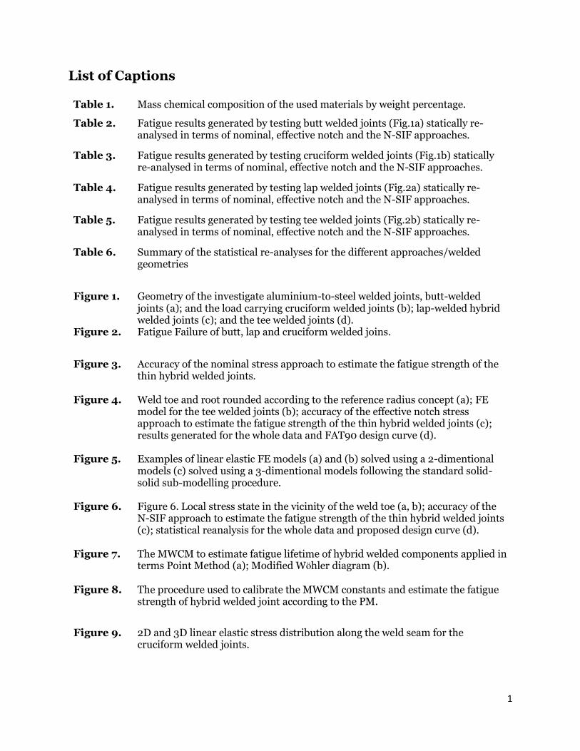
List of Captions Table 1. Mass chemical composition of the used materials by weight percentage.

Table 2. Fatigue results generated by testing butt welded joints (Fig.1a) statically re-analysed in terms of nominal, effective notch and the N-SIF approaches.

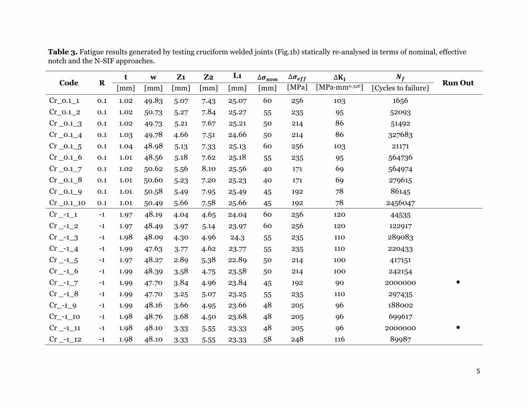
Table 3. Fatigue results generated by testing cruciform welded joints (Fig.1b) statically re-analysed in terms of nominal, effective notch and the N-SIF approaches.

Table 4. Fatigue results generated by testing lap welded joints (Fig.2a) statically re-analysed in terms of nominal, effective notch and the N-SIF approaches.

Table 5. Fatigue results generated by testing tee welded joints (Fig.2b) statically re-analysed in terms of nominal, effective notch and the N-SIF approaches.

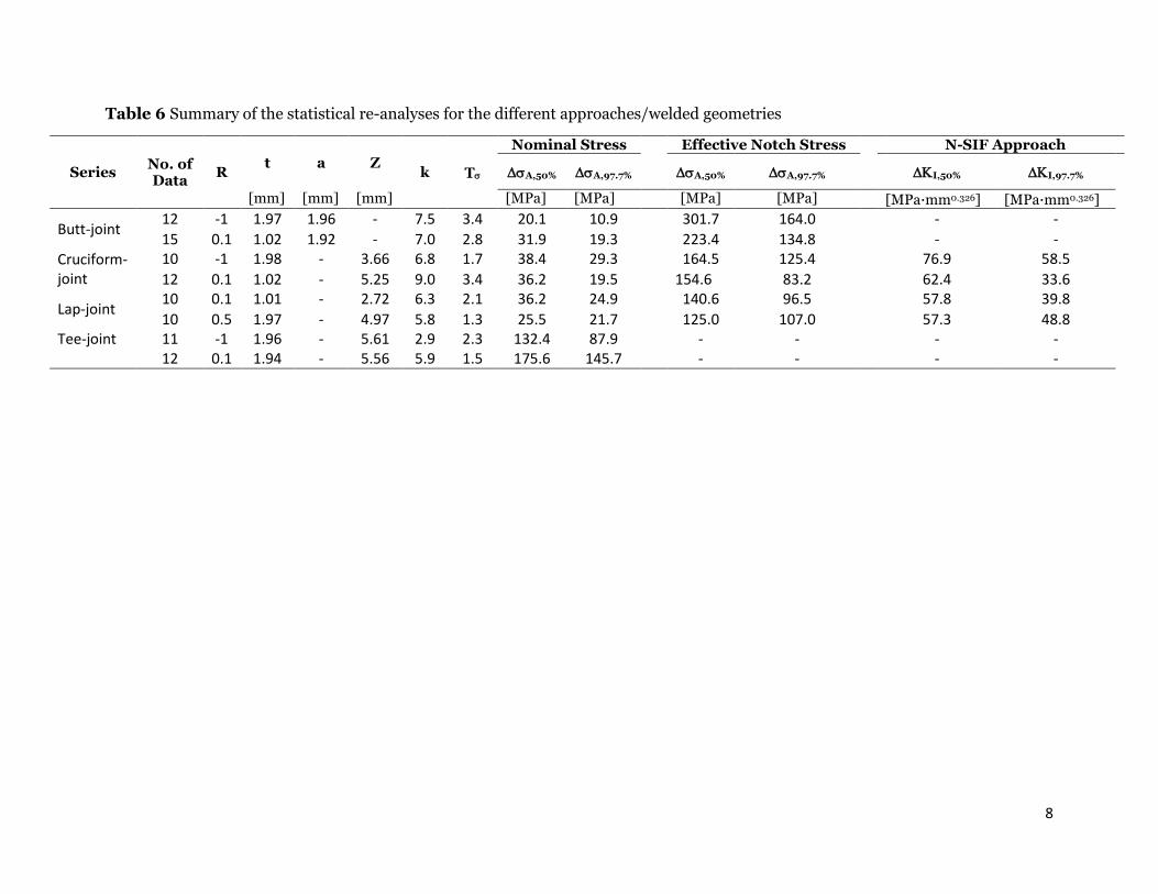
Table 6. Summary of the statistical re-analyses for the different approaches/welded geometries

Figure 1. Geometry of the investigate aluminium-to-steel welded joints, butt-welded

joints (a); and the load carrying cruciform welded joints (b); lap-welded hybrid welded joints (c); and the tee welded joints (d).

Figure 2. Fatigue Failure of butt, lap and cruciform welded joins.

Figure 3. Accuracy of the nominal stress approach to estimate the fatigue strength of the thin hybrid welded joints.

Figure 4. Weld toe and root rounded according to the reference radius concept (a); FE model for the tee welded joints (b); accuracy of the effective notch stress approach to estimate the fatigue strength of the thin hybrid welded joints (c); results generated for the whole data and FAT90 design curve (d).

Figure 5. Examples of linear elastic FE models (a) and (b) solved using a 2-dimentional models (c) solved using a 3-dimentional models following the standard solid-solid sub-modelling procedure.

Figure 6. Figure 6. Local stress state in the vicinity of the weld toe (a, b); accuracy of the N-SIF approach to estimate the fatigue strength of the thin hybrid welded joints (c); statistical reanalysis for the whole data and proposed design curve (d).

Figure 7. The MWCM to estimate fatigue lifetime of hybrid welded components applied in terms Point Method (a); Modified Wöhler diagram (b).

Figure 8. The procedure used to calibrate the MWCM constants and estimate the fatigue strength of hybrid welded joint according to the PM.

Figure 9. 2D and 3D linear elastic stress distribution along the weld seam for the cruciform welded joints.

2

Figure 10. Accuracy of the MWCM applied along with the Point Method in estimating fatigue strength of thin hybrid welded components (2D FE models).

Figure 11. Accuracy of the MWCM applied along with the Point Method in estimating fatigue

strength of thin hybrid welded components (3D FE models).

3

Tables Table 1. Mass chemical composition of the used materials by weight percentage.

Alloy Chemical composition [weight%]

AA1050 Cu Mg Si Fe Mn Zn Ti Al

0-0.05 0-0.05 0.25 0-0.4 0.05 0.07 0-0.05 Balanced

EN10130:199 C P S Mn Fe

0.12 0.045 0.045 0.60 Balanced

AA4043 Cu Mg Si Fe Mn Zn Ti Al

0.01 0.05 4.5-6.0 0.80 0.05 0.1 0.2 Balanced

4

Table 2. Fatigue results generated by testing butt welded joints (Fig.1a) statically re-analysed in

terms of nominal stress and effective notch stress approaches.

Code R t W a ∆𝝈𝒏𝒐𝒎 ∆𝝈𝒆𝒇𝒇 𝑵𝒇

Run Out [mm] [mm] [mm] [MPa] [MPa] [Cycles to failure]

Butt_0.1_1 0.1 0.99 49.00 1.88 60 420 15617

Butt_0.1_2 0.1 1.10 49.80 1.60 50 350 2000000 ●

Butt_0.1_3 0.1 1.00 50.80 1.89 54 378 289490

Butt_0.1_4 0.1 1.02 49.92 2.10 57 399 89952

Butt_0.1_5 0.1 1.03 50.05 2.17 57 399 105241

Butt_0.1_6 0.1 1.01 49.73 2.14 54 378 14380

Butt_0.1_7 0.1 1.01 50.43 1.92 52 364 23470

Butt_0.1_8 0.1 1.03 49.85 1.66 50 350 23335

Butt_0.1_9 0.1 1.01 50.34 1.82 50 350 138007

Butt_0.1_10 0.1 1.02 49.97 1.96 60 420 15275

Butt_0.1_11 0.1 1.04 50.67 1.78 50 350 67660

Butt_0.1_12 0.1 1.03 49.84 1.88 50 350 36631

Butt_0.1_13 0.1 1.03 49.50 1.97 35 245 837329

Butt_0.1_14 0.1 1.00 49.41 2.10 40 280 2000000 ●

Butt_0.1_15 0.1 1.01 49.84 1.88 45 315 967279

Butt_-1_1 -1 1.96 49.21 2.21 35 525 235783

Butt_-1_2 -1 1.96 49.12 1.92 42 630 2327

Butt_-1_3 -1 1.95 49.07 1.79 32 480 138731

Butt_-1_4 -1 1.97 49.27 2.01 35 525 6415

Butt_-1_5 -1 1.97 49.32 2.13 30 450 162306

Butt_-1_6 -1 1.98 50.41 1.87 28 420 2000000 ●

Butt_-1_7 -1 1.98 50.41 1.83 40 600 25032

Butt_-1_8 -1 1.96 50.45 1.83 32 480 2000000 ●

Butt_-1_9 -1 1.96 49.21 1.68 35 525 54914

Butt_-1_10 -1 1.99 50.24 2.00 28 420 2000000 ●

Butt_-1_11 -1 1.99 50.24 2.13 38 570 9857

Butt_-1_12 -1 1.98 50.25 2.09 28 420 41366

5

Table 3. Fatigue results generated by testing cruciform welded joints (Fig.1b) statically re-analysed in terms of nominal, effective

notch and the N-SIF approaches.

Code R t w Z1 Z2 L1 ∆𝝈𝒏𝒐𝒎 ∆𝝈𝒆𝒇𝒇 ∆𝐊𝐈 𝑵𝒇

Run Out [mm] [mm] [mm] [mm] [mm] [mm] [MPa] [MPa·mm0.326] [Cycles to failure]

Cr_0.1_1 0.1 1.02 49.83 5.07 7.43 25.07 60 256 103 1656

Cr_0.1_2 0.1 1.02 50.73 5.27 7.84 25.27 55 235 95 52093

Cr _0.1_3 0.1 1.02 49.73 5.21 7.67 25.21 50 214 86 51492

Cr _0.1_4 0.1 1.03 49.78 4.66 7.51 24.66 50 214 86 327683

Cr _0.1_5 0.1 1.04 48.98 5.13 7.33 25.13 60 256 103 21171

Cr _0.1_6 0.1 1.01 48.56 5.18 7.62 25.18 55 235 95 564736

Cr _0.1_7 0.1 1.02 50.62 5.56 8.10 25.56 40 171 69 564974

Cr _0.1_8 0.1 1.01 50.60 5.23 7.20 25.23 40 171 69 279615

Cr _0.1_9 0.1 1.01 50.58 5.49 7.95 25.49 45 192 78 86145

Cr _0.1_10 0.1 1.01 50.49 5.66 7.58 25.66 45 192 78 2456047

Cr _-1_1 -1 1.97 48.19 4.04 4.65 24.04 60 256 120 44535

Cr _-1_2 -1 1.97 48.49 3.97 5.14 23.97 60 256 120 122917

Cr _-1_3 -1 1.98 48.09 4.30 4.96 24.3 55 235 110 289083

Cr _-1_4 -1 1.99 47.63 3.77 4.62 23.77 55 235 110 220433

Cr _-1_5 -1 1.97 48.27 2.89 5.38 22.89 50 214 100 417151

Cr _-1_6 -1 1.99 48.39 3.58 4.75 23.58 50 214 100 242154

Cr _-1_7 -1 1.99 47.70 3.84 4.96 23.84 45 192 90 2000000 ●

Cr _-1_8 -1 1.99 47.70 3.25 5.07 23.25 55 235 110 297435

Cr_-1_9 -1 1.99 48.16 3.66 4.95 23.66 48 205 96 188002

Cr_-1_10 -1 1.98 48.76 3.68 4.50 23.68 48 205 96 699617

Cr _-1_11 -1 1.98 48.10 3.33 5.55 23.33 48 205 96 2000000 ●

Cr _-1_12 -1 1.98 48.10 3.33 5.55 23.33 58 248 116 89987

6

Table 4. Fatigue results generated by testing lap welded joints (Fig.2a) statically re-analysed in terms of nominal, effective notch and

the N-SIF approaches.

Code R t w Z1 Z2 L1 L2 ∆𝝈𝒏𝒐𝒎 ∆𝝈𝒆𝒇𝒇 ∆𝐊𝐈 𝑵𝒇

Run Out [mm] [mm] [mm] [mm] [mm] [mm] [MPa] [MPa] [MPa·mm0.32] [Cycles to failure]

Lap_0.1_1 0.1 1.02 50.11 2.92 2.83 22.92 22.83 60 234 96 31581

Lap_0.1_2 0.1 1.01 50.21 3.03 3.15 23.03 23.15 60 234 96 102426

Lap_0.1_3 0.1 1.01 50.20 2.42 2.37 22.42 22.37 65 253 104 94739

Lap_0.1_4 0.1 1.03 50.14 2.73 2.44 22.73 22.44 65 253 104 55703

Lap_0.1_5 0.1 1.01 50.09 2.53 2.63 22.53 22.63 55 214 88 86888

Lap_0.1_6 0.1 1.02 50.29 3.02 2.80 23.02 22.8 55 214 88 94390

Lap_0.1_7 0.1 0.98 50.17 2.79 2.55 22.79 22.55 50 195 80 367625

Lap_0.1_8 0.1 1.00 50.28 2.61 2.97 22.61 22.97 45 175 72 191873

Lap_0.1_9 0.1 1.01 50.17 2.53 2.64 22.53 22.64 45 175 72 1131920

Lap_0.1_10 0.1 1.00 50.10 2.66 2.70 22.66 22.7 50 195 80 496799

Lap_0.5_1 0.5 1.98 51.73 4.89 5.15 24.89 25.15 30 147 67 1093169

Lap_0.5_2 0.5 1.97 50.34 4.36 5.46 24.36 25.46 35 172 79 275251

Lap_0.5_3 0.5 1.98 51.82 4.58 5.60 24.58 25.6 35 172 79 209757

Lap_0.5_4 0.5 1.97 51.75 4.11 6.28 24.11 26.28 30 147 67 929710

Lap_0.5_5 0.5 1.97 51.73 6.13 4.10 26.13 24.1 32 157 72 467257

Lap_0.5_6 0.5 1.98 50.48 5.40 3.98 25.4 23.98 32 157 72 531450

Lap_0.5_7 0.5 1.97 51.76 6.27 4.83 26.27 24.83 28 137 63 2000000 ●

Lap_0.5_8 0.5 1.97 50.50 5.04 4.35 25.04 24.35 38 186 85 247044

Lap_0.5_9 0.5 1.97 51.57 4.14 4.99 24.14 24.99 38 186 85 253922

Lap_0.5_10 0.5 1.98 50.32 4.81 5.91 24.81 25.91 28 137 63 1037289

7

Table 5. Fatigue results generated by testing tee welded joints (Fig.2b) statically re-analysed in terms of nominal, effective notch and

the N-SIF approaches.

Code R t t1 w Z1 Z2 L ∆𝝈𝒏𝒐𝒎 𝑵𝒇

Run Out [mm] [mm] [mm] [mm] [mm] [mm] [mm] [cycles to failure]

Tee_0.1_1 0.1 0.99 1.94 50.14 5.75 9.26 25.75 200 634101

Tee_0.1_2 0.1 1.01 1.93 50.14 5.66 8.85 25.66 200 357228

Tee_0.1_3 0.1 1.00 1.94 49.97 5.75 8.42 25.75 180 1001833

Tee_0.1_4 0.1 0.98 1.95 49.88 5.24 7.85 25.24 180 1074989

Tee_0.1_5 0.1 1.00 1.92 49.66 6.09 8.77 26.09 210 545593

Tee_0.1_6 0.1 0.98 1.92 50.13 5.15 7.51 25.15 210 2000000 ●

Tee_0.1_7 0.1 1.00 1.92 50.13 5.15 7.51 25.15 240 731154

Tee_0.1_8 0.1 1.00 1.94 50.13 5.72 8.25 25.72 220 429920

Tee_0.1_9 0.1 0.98 1.94 49.70 5.57 8.89 25.57 220 534240

Tee_0.1_10 0.1 1.00 1.95 49.99 5.25 8.54 25.25 230 348954

Tee_0.1_11 0.1 1.02 1.94 49.77 5.77 8.04 25.77 230 269310

Tee_0.1_12 0.1 1.08 1.93 49.58 5.67 8.02 25.67 210 419127

Tee_-1_1 -1 1.03 1.96 50.01 5.47 8.11 25.47 220 498691

Tee_-1_2 -1 1.04 1.96 49.89 5.67 9.33 25.67 220 562767

Tee_-1_3 -1 1.01 1.96 50.21 5.51 8.52 25.51 210 426377

Tee_-1_4 -1 1.06 1.95 50.13 5.75 8.42 25.75 190 994315

Tee_-1_5 -1 1.08 1.95 49.90 5.81 7.41 25.81 200 1074229

Tee_-1_6 -1 1.02 1.97 49.98 6.02 8.43 26.02 190 1651181

Tee_-1_7 -1 1.08 1.95 50.01 5.09 7.54 25.09 240 260375

Tee_-1_8 -1 1.00 1.96 49.98 5.18 8.66 25.18 240 257386

Tee_-1_9 -1 1.03 1.95 50.27 5.83 7.94 25.83 230 847412

Tee_-1_10 -1 1.02 1.95 48.67 5.79 8.15 25.79 230 400377

Tee_-1_11 -1 1.01 1.97 50.00 5.60 8.52 25.60 210 694024

8

Table 6 Summary of the statistical re-analyses for the different approaches/welded geometries

Series No. of Data

R t a Z

k T

Nominal Stress

Effective Notch Stress

N-SIF Approach

A,50% A,97.7%

A,50% A,97.7% I,50% I,97.7%

[mm] [mm] [mm] [MPa] [MPa] [MPa] [MPa] [MPa·mm0.326] [MPa·mm0.326]

Butt-joint 12 -1 1.97 1.96 - 7.5 3.4 20.1 10.9 301.7 164.0 - -

15 0.1 1.02 1.92 - 7.0 2.8 31.9 19.3 223.4 134.8 - -

Cruciform-

joint

10 -1 1.98 - 3.66 6.8 1.7 38.4 29.3 164.5 125.4 76.9 58.5

12 0.1 1.02 - 5.25 9.0 3.4 36.2 19.5 154.6 83.2 62.4 33.6

Lap-joint 10 0.1 1.01 - 2.72 6.3 2.1 36.2 24.9 140.6 96.5 57.8 39.8

10 0.5 1.97 - 4.97 5.8 1.3 25.5 21.7 125.0 107.0 57.3 48.8

Tee-joint 11 -1 1.96 - 5.61 2.9 2.3 132.4 87.9 - - - -

12 0.1 1.94 - 5.56 5.9 1.5 175.6 145.7 - - - -

9

Figures (a)

(b)

(c)

(d)

Figure 1. Geometry of the investigated aluminium-to-steel welded joints, butt-welded joints (a); and the load carrying cruciform

welded joints (b); lap-welded hybrid welded joints (c); and the tee welded joints (d).

10

Butt welded joint Lap welded joint Cruciform welded

joint

Figure 2. Fatigue Failure of butt, lap and cruciform welded joins.

11

(a)

(b)

(c)

(d)

Figure 3. Accuracy of the nominal stress approach to estimate the fatigue strength of the thin

hybrid welded joints.

1

10

100

10000 100000 1000000 10000000

Nf [Cycles]

R=-1

R=0.1

∆𝝈 𝒏𝒐𝒎 [MPa]

Butt-welded Joint

𝑵𝒇 SteelAA1050

Run-OutEC9k=3.4, Δσ97 .7%=18 MPa

EC9 k=5, Δσ9 7 .7%=18 MPa

IIWk=3, Δσ95%=12 MPa

IIWk=5, Δσ9 5%=12 MPA

10

100

10000 100000 1000000 10000000

Nf [Cycles]

R=-1

R=0.1

∆𝝈 𝒏𝒐𝒎 [MPa]

Cruciform-Welded Joint

𝑵𝒇 AA1050

Ste

elAA1050

Run-Out

EC9k=3.4, Δσ97 .7%=22 MPa

EC9 k=5, Δσ9 7 .7%=22 MPa

IIWk=3, Δσ95%=22 MPa

IIWk=5, Δσ9 5%=22 MPA

10

100

10000 100000 1000000 10000000

Nf [Cycles]

R=0.5

R=0.1

∆𝝈 𝒏𝒐𝒎 [MPa]

Lap-Welded Joint

𝑵𝒇

Run-Out

AA1050Steel

EC9k=3.4, Δσ97 .7%=23 MPa

EC9k=5, Δσ9 7 .7%=23 MPa

IIWk=3, Δσ95%=22 MPa

IIWk=5, Δσ9 5%=22 MPa

10

100

100000 1000000 10000000

Nf [Cycles]

R=-1

R=0.1

∆𝝈 𝒏𝒐𝒎 [MPa]

Tee-Welded Joint

𝑵𝒇 Steel

AA

10

50

Run-OutEC3k=3.4, Δσ97 .7%=80 MPa

EC3 k=5, Δσ9 7 .7%=80 MPa

IIWk=3, Δσ95%=71 MPa

IIWk=5, Δσ9 5%=71 MPA

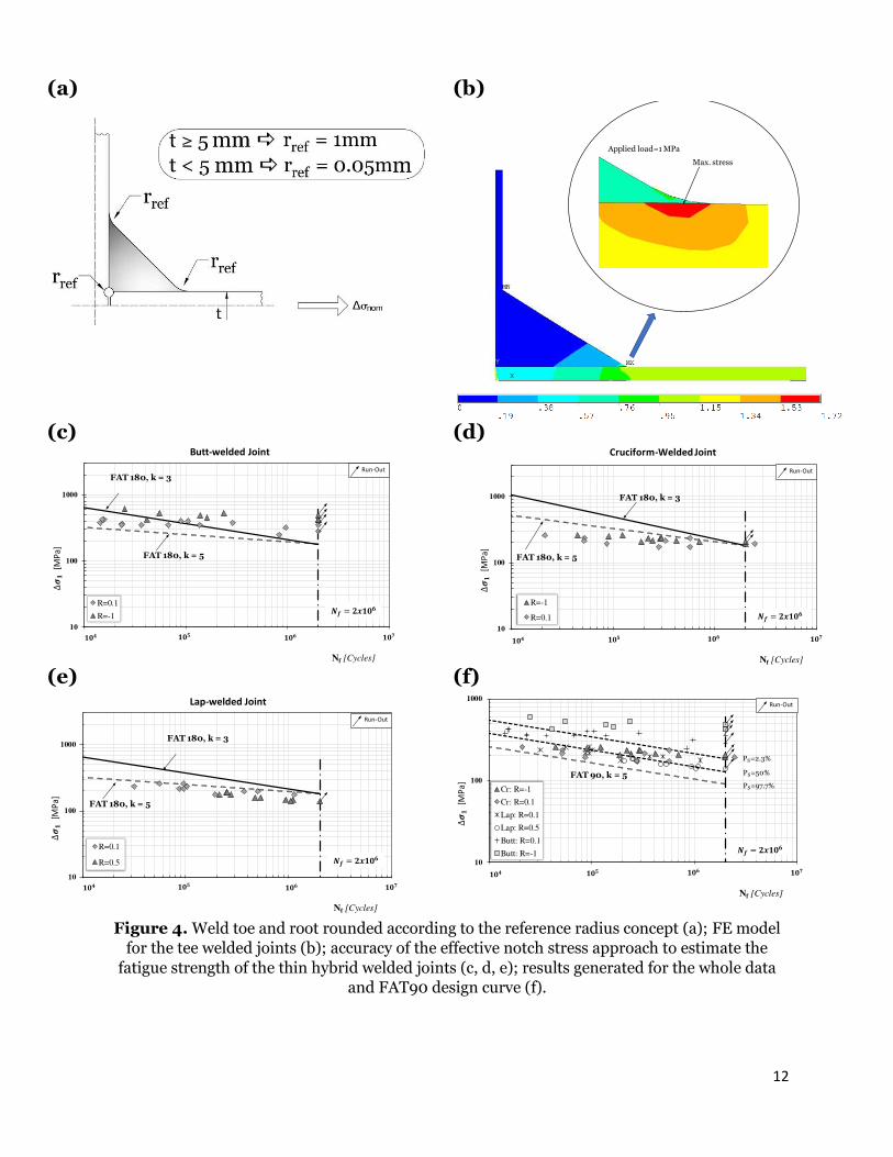
12

Figure 4. Weld toe and root rounded according to the reference radius concept (a); FE model

for the tee welded joints (b); accuracy of the effective notch stress approach to estimate the

fatigue strength of the thin hybrid welded joints (c, d, e); results generated for the whole data

and FAT90 design curve (f).

(a) (b)

(c) (d)

(e) (f)

Max. stress

Applied load=1 MPa

10

100

1000

10000 100000 1000000 1000000

Nf [Cycles]

R=0.1

R=-1

∆𝝈 [MP

a]

Butt-welded Joint

𝑵𝒇

Run-Out

FAT 180, k = 5

FAT 180, k = 3

10

100

1000

10000 100000 1000000 100000

Nf [Cycles]

R=-1

R=0.1

∆𝝈 [MP

a]

Cruciform-Welded Joint

𝑵𝒇

Run-Out

FAT 180, k = 5

FAT 180, k = 3

10

100

1000

10000 100000 1000000 1000000

Nf [Cycles]

R=0.1

R=0.5

∆𝝈 [MP

a]

Lap-welded Joint

𝑵𝒇

Run-Out

FAT 180, k = 5

FAT 180, k = 3

10

100

1000

10000 100000 1000000 1000000

Nf [Cycles]

Cr: R=-1

Cr: R=0.1

Lap: R=0.1

Lap: R=0.5

Butt: R=0.1

Butt: R=-1

∆𝝈 [MP

a]

𝑵𝒇

Run-Out

FAT 90, k = 5 PS=50%

PS=2.3%

PS=97.7%

13

(a) 2D Effective notch stress FE models

(b) 2D TCD and N-SIF FE models

(c) 3D TCD FE Complete model Sub-model

Figure 5. Examples of linear elastic FE models (a) and (b) solved using a 2-dimentional models (c) solved using a 3-dimentional models following the standard solid-solid sub-modelling

procedure.

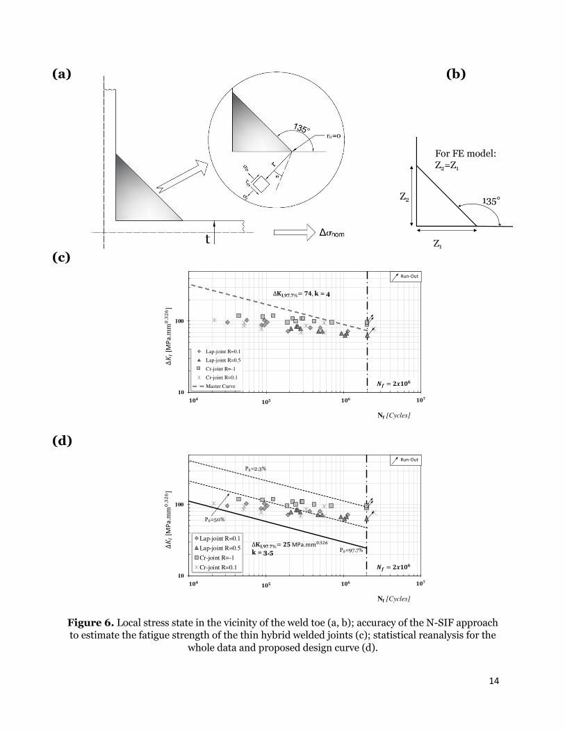
14

(a)

(b)

(c)

(d)

Figure 6. Local stress state in the vicinity of the weld toe (a, b); accuracy of the N-SIF approach

to estimate the fatigue strength of the thin hybrid welded joints (c); statistical reanalysis for the

whole data and proposed design curve (d).

10

100

10000 100000 1000000 10000000

Nf [Cycles]

Lap-joint R=0.1

Lap-joint R=0.5

Cr-joint R=-1

Cr-joint R=0.1

Master Curve

∆ [MP

a.

]

𝑵𝒇

Run-Out∆𝐊𝐈 k = 4

10

100

10000 100000 1000000 10000000

Nf [Cycles]

Lap-joint R=0.1

Lap-joint R=0.5

Cr-joint R=-1

Cr-joint R=0.1

∆ [MP

a.

]

𝑵𝒇

Run-Out

∆𝐊𝐈 k = 3.5

PS=50%

PS=2.3%

PS=97.7%

Z1

Z2 135 For FE model: Z2=Z1

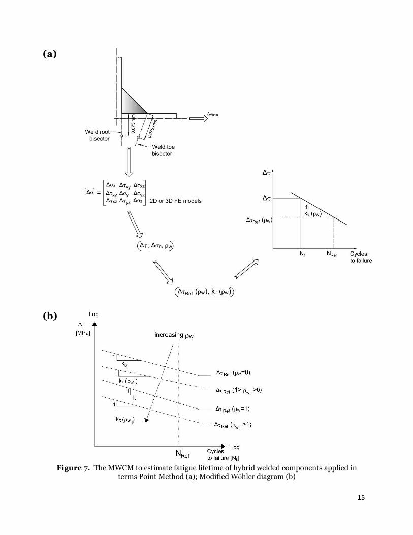
15

(a)

(b)

Figure 7. The MWCM to estimate fatigue lifetime of hybrid welded components applied in

terms Point Method (a); Modified Wöhler diagram (b)

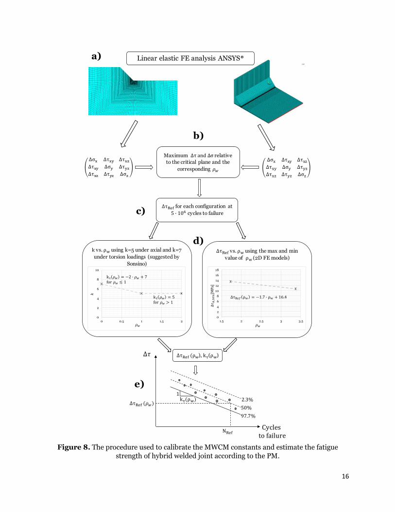
16

Figure 8. The procedure used to calibrate the MWCM constants and estimate the fatigue

strength of hybrid welded joint according to the PM.

∆ ∆ ∆ ∆ ∆ ∆ ∆ ∆ ∆ ∆ ∆ ∆ ∆ ∆ ∆ ∆ ∆ ∆

Linear elastic FE analysis ANSYS®

∆ for each configuration at cycles to failure

∆ vs. using the max and min

value of (2D FE models)

vs. using k=5 under axial and k=7

under torsion loadings (suggested by

Sonsino)

∆ ), ( )

∆

∆

1

Maximum ∆ ∆ relative

to the critical plane and the

corresponding

a)

b)

c)

d)

e)

0

2

4

6

8

10

12

14

16

18

1.5 2 2.5 3 3.5

∆

∆ 0

2

4

6

8

10

0 0.5 1 1.5 2

17

Figure 9. 2D and 3D linear elastic stress distribution along the weld seam for the cruciform welded joints.

60

65

70

75

80

85

90

95

100

0 5 10 15 20 25 30

Δσ 1

[MP

a]

Distance, [mm]

Cruciform Joint: t=1mm

Weld seammid-section

3D linear elastic-stress distrabiution

2D linear elastic-stress distrabiution

75

80

85

90

95

100

105

110

0 5 10 15 20 25 30

Δσ 1

[MP

a]

Distance, [mm]

Cruciform Joint: t=2mm

Weld seammid-section

3D linear elastic-stress distrabiution

2D linear elastic-stress distrabiution

60

65

70

75

80

85

90

0 0.1 0.2 0.3 0.4 0.5 0.6 0.7 0.8

Δσ 1

[MP

a]

Distance, [mm]

0.075 mm

75

80

85

90

95

100

105

0 0.1 0.2 0.3 0.4 0.5 0.6 0.7 0.8Δσ 1

[MP

a]

Distance, [mm]

0.075 mm

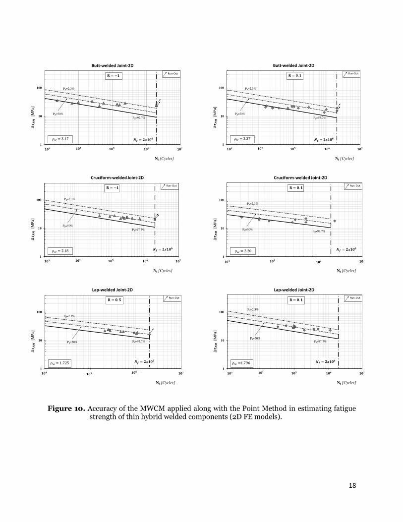
18

Figure 10. Accuracy of the MWCM applied along with the Point Method in estimating fatigue strength of thin hybrid welded components (2D FE models).

1

10

100

1000 10000 100000 1000000 10000000

Nf [Cycles]

∆ [M

Pa

]

Butt-welded Joint-2D

𝑵𝒇

Run-Out

PS=50%

PS=2.3%

PS=97.7%

1

10

100

1000 10000 100000 1000000 10000000

Nf [Cycles]

∆ [M

Pa

]

Butt-welded Joint-2D

𝑵𝒇

Run-Out

PS=50%

PS=2.3%

PS=97.7%

1

10

100

1000 10000 100000 1000000 10000000

Nf [Cycles]

∆ [M

Pa

]

Cruciform-welded Joint-2D

𝑵𝒇

Run-Out

PS=50%

PS=2.3%

PS=97.7%

1

10

100

10000 100000 1000000 10000000

Nf [Cycles]

∆ [M

Pa

]

Cruciform-welded Joint-2D

𝑵𝒇

Run-Out

PS=50%

PS=2.3%

PS=97.7%

1

10

100

10000 100000 1000000 10000000

Nf [Cycles]

∆ [M

Pa

]

Lap-welded Joint-2D

𝑵𝒇

Run-Out

PS=50%

PS=2.3%

PS=97.7%

1

10

100

1000 10000 100000 1000000 10000000

Nf [Cycles]

∆ [M

Pa

]

Lap-welded Joint-2D

𝑵𝒇

Run-Out

1.796

PS=50%

PS=2.3%

PS=97.7%

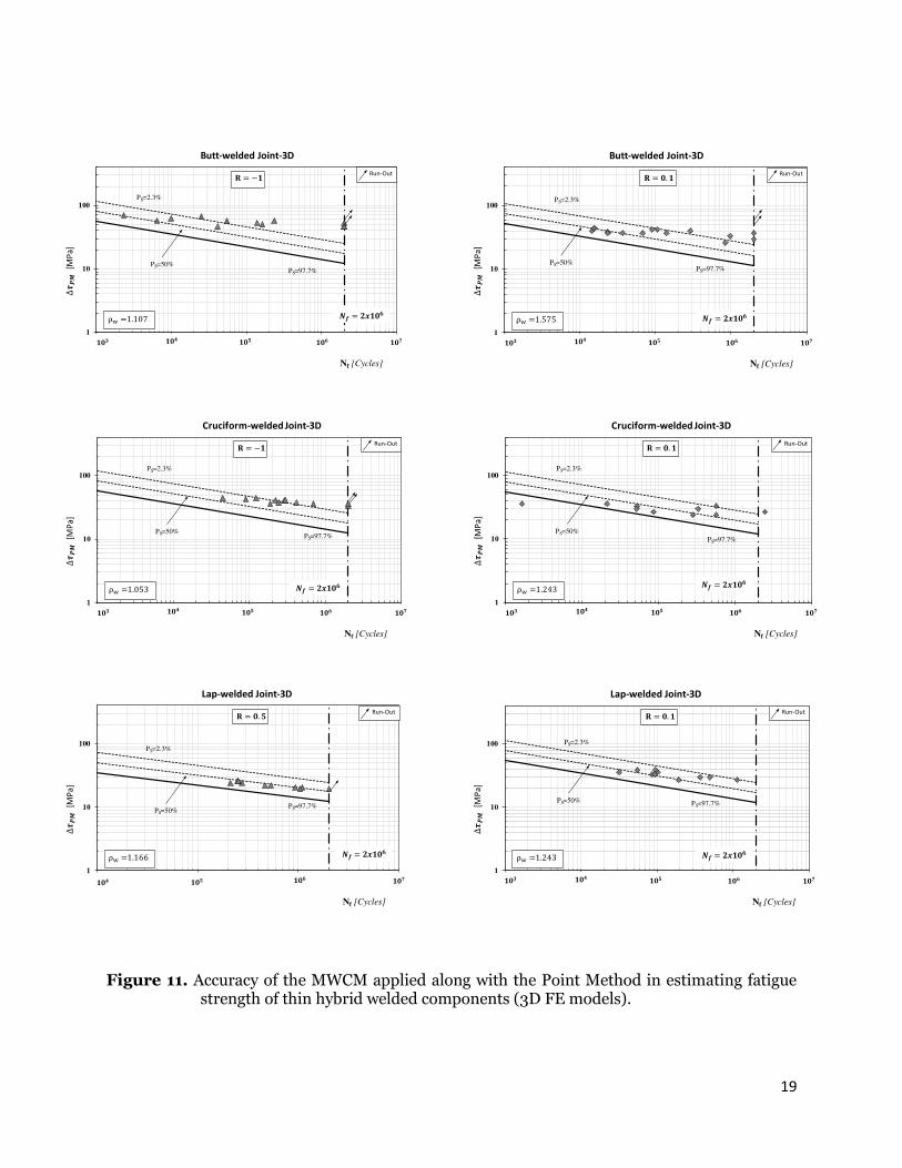
19

Figure 11. Accuracy of the MWCM applied along with the Point Method in estimating fatigue strength of thin hybrid welded components (3D FE models).

1

10

100

1000 10000 100000 1000000 10000000

Nf [Cycles]

∆ [M

Pa

]

Butt-welded Joint-3D

𝑵𝒇

Run-Out

1.107

PS=50%

PS=2.3%

PS=97.7%

1

10

100

1000 10000 100000 1000000 10000000

Nf [Cycles]

∆ [M

Pa

]

Butt-welded Joint-3D

𝑵𝒇

Run-Out

1.575

PS=50%

PS=2.3%

PS=97.7%

1

10

100

1000 10000 100000 1000000 10000000

Nf [Cycles]

∆ [M

Pa

]

Cruciform-welded Joint-3D

𝑵𝒇

Run-Out

1.053

PS=50%

PS=2.3%

PS=97.7%

1

10

100

1000 10000 100000 1000000 10000000

Nf [Cycles]

∆ [M

Pa

]

Cruciform-welded Joint-3D

𝑵𝒇

Run-Out

1.243

PS=50%

PS=2.3%

PS=97.7%

1

10

100

10000 100000 1000000 10000000

Nf [Cycles]

∆ [M

Pa

]

Lap-welded Joint-3D

𝑵𝒇

Run-Out

1.166

PS=50%

PS=2.3%

PS=97.7%

1

10

100

1000 10000 100000 1000000 10000000

Nf [Cycles]

∆ [M

Pa

]

Lap-welded Joint-3D

𝑵𝒇

Run-Out

1.243

PS=50%

PS=2.3%

PS=97.7%