Embed Size (px)
Citation preview
NOISE REDUCTION OF 15-LEAD
ELECTROCARDIOGRAM SIGNALS USING SIGNAL
PROCESSING ALGORITHMS
By
WEI LIU
Bachelor of Science
Tianjin University
Tianjin, China
2005
Submitted to the Faculty of the Graduate College of the
Oklahoma State University in partial fulfillment of
the requirements for the Degree of
MASTER OF SCIENCE July, 2007
ii
NOISE REDUCTION OF 15-LEAD
ELECTROCARDIOGRAM SIGNALS USING SIGNAL
PROCESSING ALGORITHMS
Thesis Approved:
Dr. Mark G. Rockley
Thesis Adviser Dr. Lionel M. Raff
Dr. Satish Bukkapatnam
Dr. A. Gordon Emslie
Dean of the Graduate College
iii
PREFACE
ECG signals are routinely contaminated by noise due to motion artifacts, power
line noise, and transducer generated noise, all of which will decrease the accuracy of
ECG spectral interpretation. Signal baseline drift may also affect the interpretation, this
being caused by respiration, and motion of the subject. This research demonstrates that
by efficient digital signal processing, much of this noise and baseline drift can be
effectively eliminated with a consequent improvement of diagnostic accuracy. The ECG
spectra are first processed by using a symmetrical triangle weighting function (ST) to
eliminate the high frequency noise. The ST smoothed data are then processed by an FIR
high pass filter to decrease baseline wander. The resulting denoised signals are then
analyzed to obtain typical ECG interpretive parameters, such as feature intervals,
magnitudes, and segment elevations. ROC (receiver operating characteristic) curves for a
specific diagnostic test for myocardial infarction are generated to demonstrate the
efficacy of the proposed noise reduction techniques. It was noted that when compared
with a Fourier transform noise reduction technique, the area under the ROC curve
increased by 20%, indicating that the digital signal processing described in this work
increased the sensitivity and specificity of the detection of this common cardio-vascular
pathology.

iv
ACKNOWLEGEMENT
I would like to express my gratitude to Dr. M. G. Rockley, my research advisor
and the chairman of my graduate committee, for his guidance of my graduate work. The
instructions in how to think and solve problems he gave have been invaluable to my
graduate experience. I would also like to thank Dr. L. M. Raff and Dr. S. Bukkapatnam,
my graduate advisory committee members, for their help and advice during my research.
Thanks are also due to Dr. R. Komanduri, Dr. M. Hagan and Dr. B. Benjamin, the
faculty members in the ECG research group, for their help with my research.
I would like to thank the Department of Chemistry for providing a teaching
assistantship to me for support during my graduate work at Oklahoma State University. I
would also like to thank Bob, Cheryl, and Carolyn in the Chemistry department office for
their assistance during my study.
Finally, I would like to express my appreciation to my family and friends. Their
continued support during the last two years has been of great help to me in finishing my
work.
v
TABLE OF CONTENTS
Chapter Page INTRODUCTION .........................................................................................................1
The Electrocardiogram...........................................................................................1 Noise in ECG signals .............................................................................................2 Noise Reduction Methods......................................................................................6
Wavelet transform..........................................................................................6 Fast Fourier transform....................................................................................8 Morphological operators................................................................................9
METHODOLOGY ......................................................................................................13
Signal Smooth......................................................................................................13
The Moving Average ...................................................................................13 Least squares fitting .....................................................................................18
FIR Filter..............................................................................................................19 Window method...........................................................................................20 Optimal method ...........................................................................................27
ROC Curve...........................................................................................................28 Binary test ....................................................................................................29 Continuous test.............................................................................................30 Ordinal Test .................................................................................................31 Obtain ROC Curves .....................................................................................32 Area under the curve....................................................................................35 Partial area under the curve..........................................................................36
RESULTS AND DISCUSSION..................................................................................37
PTB diagnostic database ......................................................................................37 Signal Processing and results...............................................................................38
Data smooth and results ...............................................................................38 FIR filter and results ....................................................................................49 Further benefits of the application of digital filters .....................................53
Feature extraction.................................................................................................57 ROC curve analysis of the ST segment elevation test .........................................58
CONCLUSION............................................................................................................64 REFERENCES ............................................................................................................66

vi
APPENDIX..................................................................................................................69

vii
LIST OF TABLES
Table Page 1. Sample data for an ROC curve ...................................................................................33
2. Content for PTB diagnostic database..........................................................................38
3. Area under the curve of different leads and different method ....................................61
viii
LIST OF FIGURES
Figure Page 1. Stylized ECG signal..............................................................................................2
2. Baseline wander due to motion artifacts in a real ECG signal .............................3
3. High frequency noise in real ECG signal .............................................................4
4. Uncertainty in parameter determination caused by high frequency noise............5
5. Illustration of convolution...................................................................................14
6. Symmetrical triangle coefficient function ..........................................................16
7. Frequency response of the triangle coefficient function.....................................16
8. Symmetrical exponential function ......................................................................17
9. Frequency response of exponential function ......................................................18
10. Ideal frequency response.....................................................................................21
11. Initial impulse response calculated from inverse FFT........................................21
12. Shift of the initial impulse response....................................................................22
13. Frequency response for different numbers of coefficients .................................23
14. Passband ripple and transition region .................................................................24
15. Calculation of impulse response by window method .........................................25
16. Frequency response with evenly distributed ripples...........................................27
17. Definition of positive and negative in continuous test by threshold...................30
18. The ROC curve plotted from Fig. 17 ..................................................................31
19. ROC curve of Table 1 .........................................................................................34
ix
Figure Page
20. Different ROC curves .........................................................................................35
21. 25 point symmetrical triangle weighting function ..............................................39
22. 25 Savitzky Golay smooth weighting function...................................................40
23. ECG spectrum segment before smooth...............................................................41
24. ECG spectrum smoothed by 25 point symmetrical triangle weighting function41
25. ECG spectrum smoothed by 25 point SG smooth ..............................................42
26. Frequency domain ECG spectrum smoothed by 25 point symmetrical triangle
weighting function ..............................................................................................43
27. Frequency domain ECG spectrum smoothed by 25 point SG smooth ...............43
28. 35 point symmetrical triangle weighting function ..............................................45
29. Frequency response of the 35 symmetrical triangle weighting function ............45
30. ECG spectrum before smooth.............................................................................46
31. ECG spectrum smoothed by a 25 symmetrical triangle function .......................46
32. Original ECG spectra in frequency domain........................................................47
33. An ECG spectrum in frequency domain processed by 5 point SG smooth ........48
34. An ECG spectrum in frequency domain processed by 21 point SG smooth ......48
35. An ECG spectrum in frequency domain processed by 35 point SG smooth ......49
36. Impulse response of designed FIR high pass filter .............................................50
x
Figure Page
37. Frequency response for designed FIR filter........................................................50
38. An original ECG spectrum with baseline wander...............................................51
39. FIR filtered ECG spectrum .................................................................................52
40. Low frequency area of ECG spectrum in frequency domain .............................52
41. Low frequency area of ECG spectrum processed by FIR high pass filter in
frequency domain................................................................................................53
42. First derivative of original ECG spectrum segment ...........................................54
43. First derivative of processed ECG spectrum segment ........................................55
44. Original ECG spectrum plotted from orthogonal bipolar leads..........................56
45. Processed ECG spectrum plotted from orthogonal bipolar leads .......................56
46. Determination of ST segment elevation .............................................................58
47. Segment of an ECG spectrum processed by algorithm proposed.......................59
48. Segment of an ECG spectrum processed by standard method ...........................60
49. ROC curves for lead V1......................................................................................61
50. ROC curves of lead V2.......................................................................................62
51. ROC curves for Lead V3 ....................................................................................62
1
CHAPTER I
INTRODUCTION
The Electrocardiogram
An electrocardiograph produces an electrocardiogram (ECG or EKG) which
records the electrical activity of the heart over time in exquisite detail. The ECG signal is
recorded by properly pasting a certain number of electrodes on the body. A typical heart
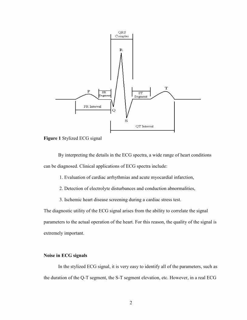
beat as recorded in the ECG spectra has three main components, referred to as the P
wave, the QRS complex and the T wave.
The P wave corresponds to the depolarization of the atrium during contraction.
The QRS complex corresponds to the depolarization of the ventricle during contraction.
The T wave corresponds to repolarization of the ventricle during expansion. The
dynamically changing shape of the beat is highly correlated with the health of the heart.
Fig. 1 shows a stylized ECG signal of one heart beat.
2
Figure 1 Stylized ECG signal
By interpreting the details in the ECG spectra, a wide range of heart conditions
can be diagnosed. Clinical applications of ECG spectra include:
1. Evaluation of cardiac arrhythmias and acute myocardial infarction,
2. Detection of electrolyte disturbances and conduction abnormalities,
3. Ischemic heart disease screening during a cardiac stress test.
The diagnostic utility of the ECG signal arises from the ability to correlate the signal
parameters to the actual operation of the heart. For this reason, the quality of the signal is
extremely important.
Noise in ECG signals
In the stylized ECG signal, it is very easy to identify all of the parameters, such as
the duration of the Q-T segment, the S-T segment elevation, etc. However, in a real ECG
3
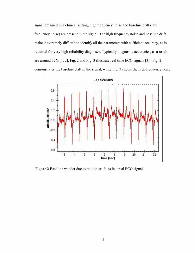
signal obtained in a clinical setting, high frequency noise and baseline drift (low
frequency noise) are present in the signal. The high frequency noise and baseline drift
make it extremely difficult to identify all the parameters with sufficient accuracy, as is
required for very high reliability diagnoses. Typically diagnostic accuracies, as a result,
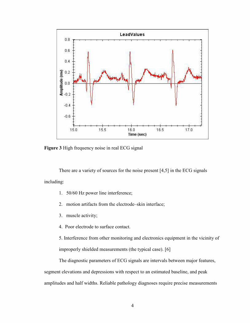
are around 72% [1, 2]. Fig. 2 and Fig. 3 illustrate real time ECG signals [3]. Fig. 2
demonstrates the baseline drift in the signal, while Fig. 3 shows the high frequency noise.
Figure 2 Baseline wander due to motion artifacts in a real ECG signal
4
Figure 3 High frequency noise in real ECG signal
There are a variety of sources for the noise present [4,5] in the ECG signals
including:
1. 50/60 Hz power line interference;
2. motion artifacts from the electrode–skin interface;
3. muscle activity;
4. Poor electrode to surface contact.
5. Interference from other monitoring and electronics equipment in the vicinity of
improperly shielded measurements (the typical case). [6]
The diagnostic parameters of ECG signals are intervals between major features,
segment elevations and depressions with respect to an estimated baseline, and peak
amplitudes and half widths. Reliable pathology diagnoses require precise measurements
5
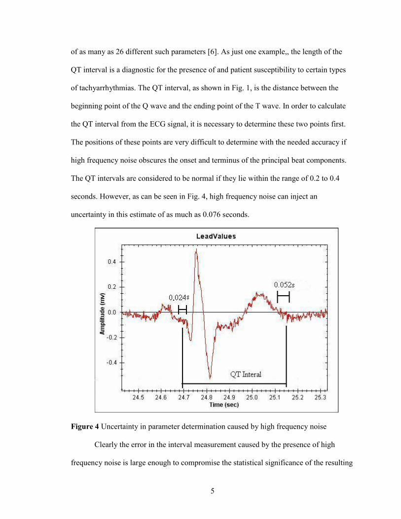
of as many as 26 different such parameters [6]. As just one example,, the length of the
QT interval is a diagnostic for the presence of and patient susceptibility to certain types
of tachyarrhythmias. The QT interval, as shown in Fig. 1, is the distance between the
beginning point of the Q wave and the ending point of the T wave. In order to calculate
the QT interval from the ECG signal, it is necessary to determine these two points first.
The positions of these points are very difficult to determine with the needed accuracy if
high frequency noise obscures the onset and terminus of the principal beat components.
The QT intervals are considered to be normal if they lie within the range of 0.2 to 0.4
seconds. However, as can be seen in Fig. 4, high frequency noise can inject an
uncertainty in this estimate of as much as 0.076 seconds.
Figure 4 Uncertainty in parameter determination caused by high frequency noise
Clearly the error in the interval measurement caused by the presence of high
frequency noise is large enough to compromise the statistical significance of the resulting
6
analysis for this particular diagnostic test. There are as many as 25 more features [7] such
as the QT interval required to adequately characterize the ECG signal for reliable medical
diagnosis. The need for improvement in reliable detection of these features is apparent.
The first and most obvious way to improve diagnostic accuracy is to remove signal noise,
without significantly altering the resulting diagnostic results.
Noise Reduction Methods
Wavelet transform
There are several methods that have been developed for ECG signal conditioning.
Wavelet transform has been widely used in signal processing for its ability to separate the
signal and noise. Recently, wavelet theory has been applied in feature extraction and
signal de-noising [8, 9]. The wavelet transform modulus method [10] and the wavelet
threshold de-noising method [11, 12] are typically used for ECG signal processing [13].
The wavelet transform modulus method is able to maximize the information present in
the original signal while minimizing noise. However, this method requires extensive
computation [14] and the general features of the ECG spectrum are removed and replaced
by a wavelet convolution of the spectrum. .
The wavelet threshold de-noising method is a coefficient selection method in
which an optimal mother wavelet filter is used as the wavelet in the discrete wavelet
transform (DWT). This DWT with optimal wavelet is applied to noisy ECG signals to
obtain wavelet coefficients at different scales in order to transform the ECG signal into
the wavelet domain. A magnitude threshold is preset to separate the smaller wavelet
coefficients corresponding to noise and the larger ones corresponding to the signal. Then
7
the coefficients that are below the threshold are replaced by zeros, effectively removing
any contributions to the signal associated with these components and thus removing the
‘noise’ due to these components of the signal. For the coefficients above the threshold,
there are two treatments: hard-thresholding which retains all the signal coefficients and
soft-thresholding which retains a portion of signal coefficients. The hard-thresholding
method is more accurate but more computationally intensive than soft-thresholding. Once
the appropriate thresholding methods have been applied, the processed coefficients and
the mother wavelet are then transformed back to the time domain using inverse wavelet
transform procedures. The wavelet threshold de-noising method is an effective ECG
signal processing method. However wavelet transforms require a large computational
capability in order to determine the wavelet coefficients at all possible scales. A more
efficient wavelet analysis can be obtained at the expense of some signal information by
selection of a subset of scales and positions.
The problem then becomes one of selecting the optimal wavelength. This is a
difficult task. B.N.Singh [15] proposed an algorithm to select a suitable mother wavelet
for the discrete wavelet transform of ECG signals by selecting the wavelet that
maximizes the coefficient values in the wavelet domain. This wavelet transform using the
optimal mother wavelet was then applied to a simulated ECG signal. This increases the
detection accuracy of characteristics waves such as QRS complex, P and T wave.
There are other important challenges to the technique of using DWT. One of
these is oscillation of the reconstructed ECG signal that may occur when the hard-
thresholding de-noising method is applied [13]. The amplitudes of ECG waveforms,
especially those of R waves, will also be reduced by the soft-thresholding DWT de-
8
noising method [13]. Moreover, the Q and R waves in the reconstructed ECG signal may
exhibit Pseudo-Gibbs phenomena in the wavelet threshold method [16, 17]. L. Su [13]
proposed an improved wavelet thresholding method and a translation-invariant wavelet
de-noising method to overcome the problems inherent in the classic wavelet thresholding
method. These methods successfully removed the artificial Gaussian white noise added to
a “clean” ECG signal.
The wavelet transform method is a very promising technique for signal processing
[18] and it provides an effective solution to ECG signal conditioning [19, 20]. However,
in the de-noising of ECG signals using wavelet theory, “the scales and the thresholds for
the non-stationary baseline correction and noise suppression cannot be selected
adaptively” [21]. O. Sayadi [22] has proposed an adaptive bionic wavelet transform to
solve this problem and much work on the use of DWT continues. However, for very
large scale processing of huge numbers of ECG signals in real time, computational
efficiency does become an issue. The search for improved DWT and alternative digital
signal processing techniques must continue. The work described here is an attempt to
address some of these issues by pursuing alternative techniques.
Fast Fourier transform
Another method for the de-noising of ECG signals is the use of the fast Fourier
transform (FFT). Typical high frequency noise is shown in Fig. 4. The baseline wander
(the low frequency noise) is shown in Fig. 5. When a Fourier transform is applied to an
ECG signal, the signal is transformed from the time domain to the frequency domain,
generating a set of amplitudes as a function of frequency. The signal is then filtered by
9
replacing the lower and higher frequency amplitudes (which correspond to the high and
low frequency noise) with zeros. This is known as ‘boxcar apodization’. Softer filters
such as triangular and Hanning apodization functions may also be applied. Then an
inverse FFT is applied to convert the filtered signal from the frequency domain back to
the time domain. This FFT method is a very simple, effective method for de-noising.
However, control over the magnitude of the amplitude of the stop-band and pass-band
ripple is somewhat limited and the method is computationally intensive. The reader may
recall that part of this work is directed towards obtaining a computationally undemanding
procedure for denoising ECG spectra.
Morphological operators
The morphological operators method is also a good choice for signal processing
due to its “robust and adaptive performance in extracting the shape information in
addition to their simple and quick sets computation” [21-25].
The morphological operators methods include four operations: erosion, dilation,
opening and closing. Erosion and dilation operations are similar to convolution. A
weighting function is defined for the operation. In the dilation operation, when the
weighting function is convolved through the whole spectrum, a point-wise addition is
performed. The maximum value of the results is then selected as the processed value. For
erosion, a pointwise subtraction is performed and the minimum value of the results is the
processed value. The signal is expanded by the dilation operation and the high frequency
noise is therefore reduced. In erosion operation, the signal is “shrunk” to reduce the
noise. Both the dilation and erosion operation can reduce the noise, however, the signal
will be distorted when being expanded or “shrunk”.
10
To solve this problem, an opening and closing operation was proposed. When an
opening operation is applied, the spectrum is processed by the erosion operation followed
by the dilation operation. The closing operation is performed by applying the dilation
operation followed by erosion operation. Therefore the distortion caused by the dilation
and erosion method can be balanced.
In the morphological operators method proposed by Delp [26], the ECG signal
was processed by the opening operation followed by the closing operation. The original
signal was processed again by the closing operation followed by the opening operation.
The two processed signal was averaged to get the optimal result. Then the peaks were
removed from the signal by the opening operation to estimate the baseline drift, the pit
left was reduced by the closing operation. The baseline wander was then decreased by
subtracting the estimated baseline drift from the smoothed ECG signal.
The opening and closing operations only partly balanced the distortion caused by
the dilation and erosion operations. Therefore, while reducing the noise, Delp’s method
distorted the information in the ECG signals [25]. For example, the ST segments area was
found to be shorter and the T wave became smaller. Sun [25] developed a modified
morphological filtering algorithm with improved weighting functions to obtain a better
signal conditioning performance. The signal distortion rate is reduced by 45% when this
improved method is applied.
In addition to these previously discussed methods, a time-warped polynomial
filter algorithm [27] and signal processing based on independent component analysis [28]
have been shown to be able to reduce the noise in the ECG signal.
11
Most of the methods mentioned above deal with real ECG signals with artificially
generated Gaussian high frequency white noise and simulated baseline drift added to the
signal, additionally, some of them use simulated ECG signals. Real ECG signals have
more complicated baseline drift and varying levels of high frequency noise. Therefore
any method for noise reduction needs to be applied on real ECG signals with real noise
and a method devised for determining whether or not they achieve increased diagnostic
accuracy. This has not been done in the studies noted in this discussion.
Typically, signal to noise ratio and the accuracy of detection are the criteria used
for evaluating the de-noising efficiency. Considering that the purpose of the ECG signal
processing is to give a more reliable diagnosis of a potentially pathological condition of a
patient’s heart, the diagnosis accuracy would be a more appropriate criterion for the
signal processing efficiency.
In order to overcome the difficulties inherent in the methods above, an ECG de-
noising algorithm is proposed in which the effectiveness of the algorithm is evaluated by
actually assessing its diagnostic accuracy. In this algorithm, the real ECG spectra (as
opposed to simulated ECG spectra with noise added as found in the work cited above are
first processed using a symmetrical triangle weighting function (ST) to reduce the high
frequency noise. The ST smoothed spectra are then processed by a FIR high pass filter to
decrease the baseline wander. The de-noised signals are then analyzed to obtain
diagnostic parameters (the intervals, segments, and elevations) that relate to the condition
of the heart. In this work, the S-T segment elevation is determined and used as a
diagnostic indicator of myocardial infarction. Receiver operating characteristic (ROC)
12
curves for the diagnostic test using the processed signals are then generated to evaluate
the performance of the algorithms applied.
13
CHAPTER II
METHODOLOGY
Signal Smooth
Savitzky and Golay have developed a digital filter that is now widely used in
infrared spectroscopy for the removal of random noise from molecular spectra. The
principles of this digital filter are well summarized in their article [29] as follows.
The spectra must meet two requirements before being smoothed by the methods.
First, the points in the chosen abscissa must have a fixed, uniform interval. In ECG
spectra, with time as the abscissa value, the amplitude is measured from ECG machines
at a fixed frequency, typically 1 kHz or 10 kHz. Therefore, each datum is “obtained at the
same time interval from each preceding point” [29]. The second restriction requires that
the function underlying the data points “be continuous and more or less smooth”.
The Moving Average
The use of a moving average is one of the simplest and most widely used ways to
smooth noisy data. A fixed number of points in the spectra is averaged. This average
value is treated as the smoothed ordinate value of points at the center of this array of
fixed points. Next, the first point in these
14
fixed points is dropped, and the point beyond the last is added, and the procedure is then
repeated.
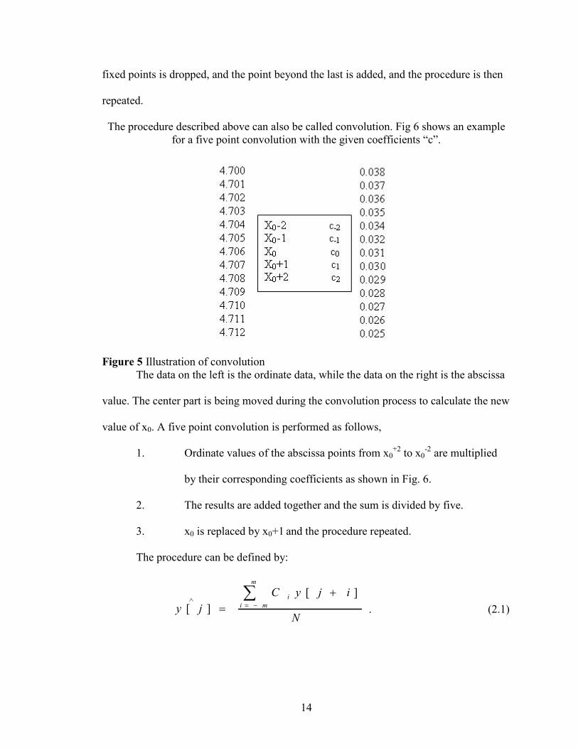
The procedure described above can also be called convolution. Fig 6 shows an example for a five point convolution with the given coefficients “c”.
Figure 5 Illustration of convolution The data on the left is the ordinate data, while the data on the right is the abscissa
value. The center part is being moved during the convolution process to calculate the new
value of x0. A five point convolution is performed as follows,
1. Ordinate values of the abscissa points from x0+2 to x0
-2 are multiplied
by their corresponding coefficients as shown in Fig. 6.
2. The results are added together and the sum is divided by five.
3. x0 is replaced by x0+1 and the procedure repeated.
The procedure can be defined by:
N
ijyCjy
m
mii∑
−=∧
+=
][][ . (2.1)
15
In the equation (2.1), ∧
][ jy stands for the convolved value, N is the scaling factor. Ci is a
set of convoluting coefficients.
For the five point moving average we mentioned, the coefficients Ci all equal one
and N equals five. The moving average is a special type of convolution in which all the
coefficients equal one. In the general case, the coefficients Ci can have any value, while
the scaling factor is determined by the number of coefficients.
In convolution, if all of the coefficients equal one, all the points around x0 have
the same weight. The scaling factor is, as already noted, the number of coefficients. This
moving average is best when the points around x0 are strongly related to X0. In molecular
and ECG spectra, this may not always be true. For example, in ECG spectra, the R wave
is very sharp. There is a large difference from one point to another in R wave. With this
type of data, the influences of the points around x0 are quite different, so weighting them
equally will lead to an inaccurately smoothed result. Therefore a different set of weighted
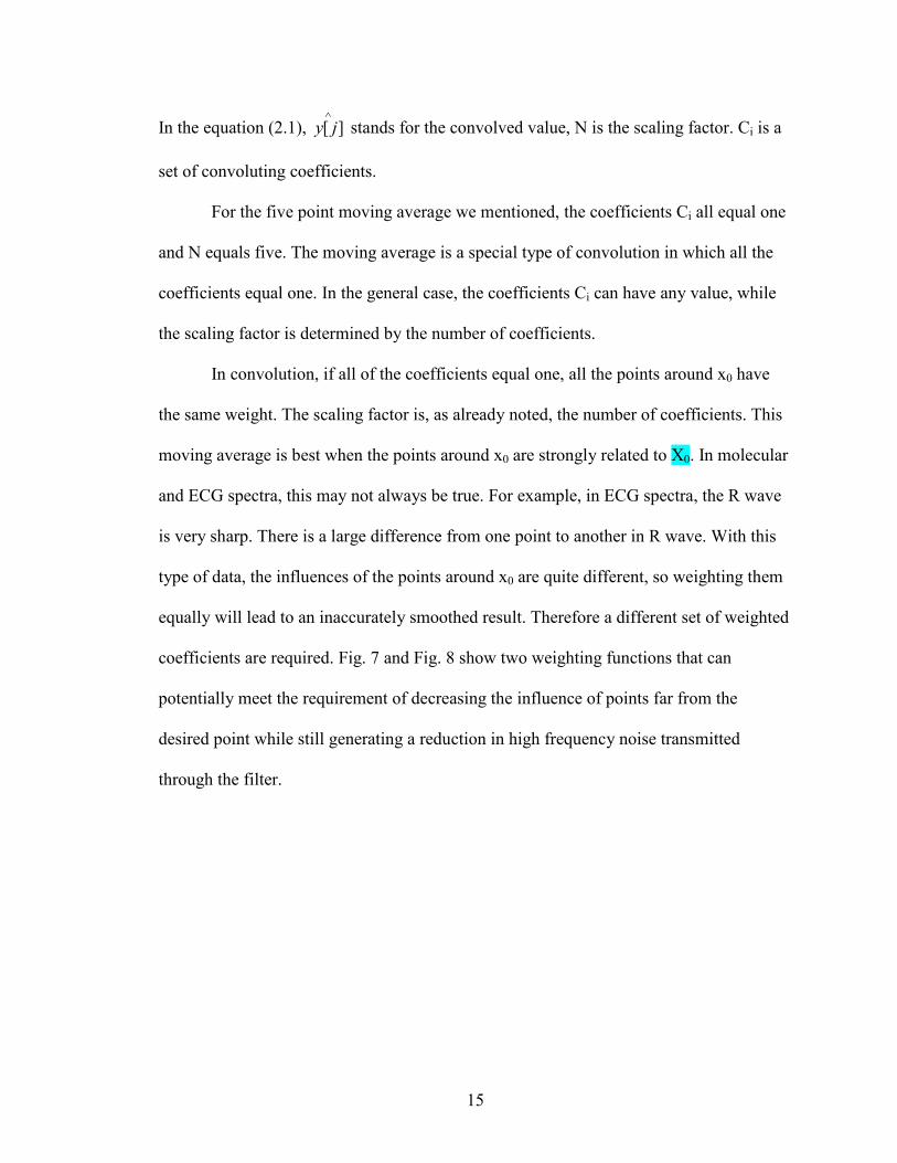
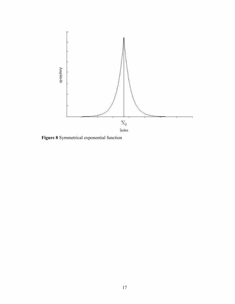
coefficients are required. Fig. 7 and Fig. 8 show two weighting functions that can
potentially meet the requirement of decreasing the influence of points far from the
desired point while still generating a reduction in high frequency noise transmitted
through the filter.
16
Figure 6 Symmetrical triangle coefficient function
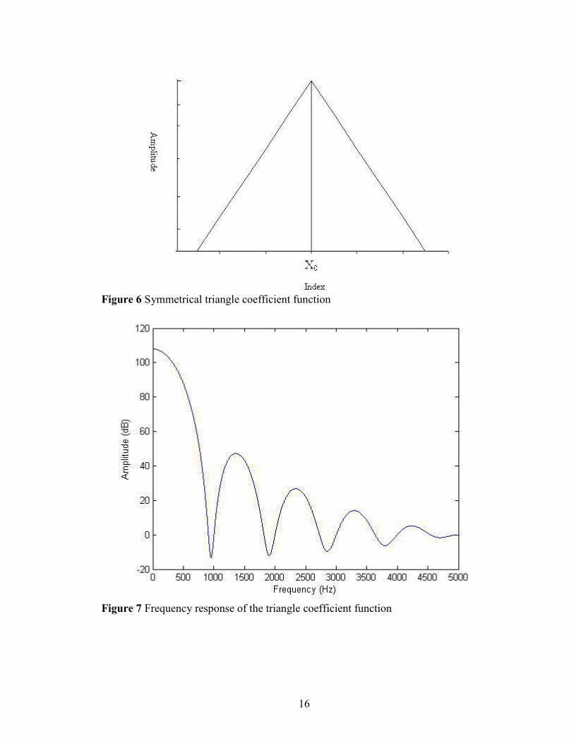
Figure 7 Frequency response of the triangle coefficient function
17
Figure 8 Symmetrical exponential function
18
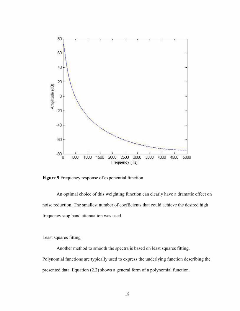
Figure 9 Frequency response of exponential function
An optimal choice of this weighting function can clearly have a dramatic effect on
noise reduction. The smallest number of coefficients that could achieve the desired high
frequency stop band attenuation was used.
Least squares fitting
Another method to smooth the spectra is based on least squares fitting.
Polynomial functions are typically used to express the underlying function describing the
presented data. Equation (2.2) shows a general form of a polynomial function.
19
∑=
=N
n
nn xay
0, (2.2)
where N is the degree of the polynomial function. N is an artificially assigned integer.
The larger the degree is, the more precise the curve is. The best fit polynomial function
will minimize the squared error.
For the treatment of spectra using the least square method, first a set of points
from the spectra is chosen. Second, the function for the best fit curve of this set of points
is determined. Finally, the central point x0 is substituted in the function of the best fit
curve to find it’s smoothed ordinate value. Then the first point of this set is dropped while
the point beyond the last point is added, and the procedure is repeated.
The least square method is computationally intensive while convoluting the
spectra with a set of coefficients is much less intensive. Furthermore, polynomial fitting
is subject to the problem of overfitting if the order of the polynomial is too high and
underfitting if the order is too low. Optimal fitting is then arbitrary and the reliability of
the outcome is poor. Savitzky and Golay carefully combined these two methods and
developed a set of coefficients which provide a weighting function. Convolution of the
spectra with the weighting function derived by Savitzky and Golay has the same result as
the least squares fitting method while reduces the computational time compared to the
least square fitting method.
FIR Filter
A much more controllable version of the digital convolution formula derived by
Savitzky and Golay may be obtained using a finite impulse response filter. For this work,
the SG filter is used to remove high frequency noise while the FIR filter is used to
20
remove low frequency noise. It should be apparent to the reader, following the
discussion below, that the SG filter is, in fact, a form of an FIR low pass filter.
The output of the signal processed by an FIR filter is calculated by convoluting
only the recent past output and current input samples. The coefficients used for the
convolution specify the generate the impulse while each coefficient is called ‘‘a tap’. For
a general M tap FIR filter, the nth output is determined by the following equation.
∑−
=
−=1
0
)()(][M
kknxkhny . (2.3)
In the equation, M is the tap of the impulse response and h(k) is the impulse response (so-
called because it is effectively the generated response if a single impulse was passed
through the FIR filter). The dominant techniques used to design the FIR filter are the
window design method and the optimal method.
Window method
The window design method (also called the Fourier series method) starts with the
desired frequency response for the filter. An ideal continuous frequency response H(f) is
defined (Fig. 10a). The continuous frequency response is then represented by a discrete
frequency response (Fig. 10b).
21
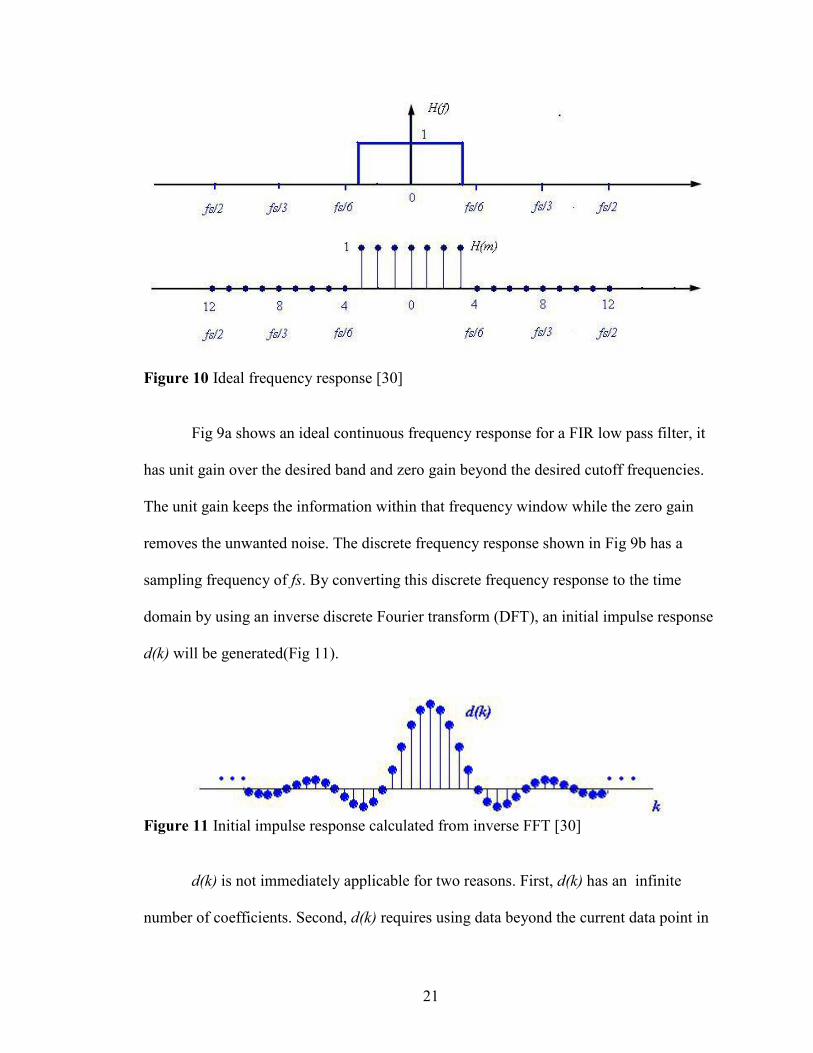
Figure 10 Ideal frequency response [30]
Fig 9a shows an ideal continuous frequency response for a FIR low pass filter, it
has unit gain over the desired band and zero gain beyond the desired cutoff frequencies.
The unit gain keeps the information within that frequency window while the zero gain
removes the unwanted noise. The discrete frequency response shown in Fig 9b has a
sampling frequency of fs. By converting this discrete frequency response to the time
domain by using an inverse discrete Fourier transform (DFT), an initial impulse response
d(k) will be generated(Fig 11).
Figure 11 Initial impulse response calculated from inverse FFT [30]
d(k) is not immediately applicable for two reasons. First, d(k) has an infinite
number of coefficients. Second, d(k) requires using data beyond the current data point in
22
the time series while the impulse response must be designed to use the current and
previous input data points. Therefore, it is necessary to shift d(k) and reduce the number
of coefficients. Fig. 12a shows the initial impulse response resulting from the inverse
DFT. Initially, up to 14 points in advance of the datum point of interest is used, those
points are the points with negative indexes shown in Fig. 12a. By shifting the initial
coefficients to the right, there are no advance points used as shown in Fig. 11b. The shift
will not change the frequency magnitude response.
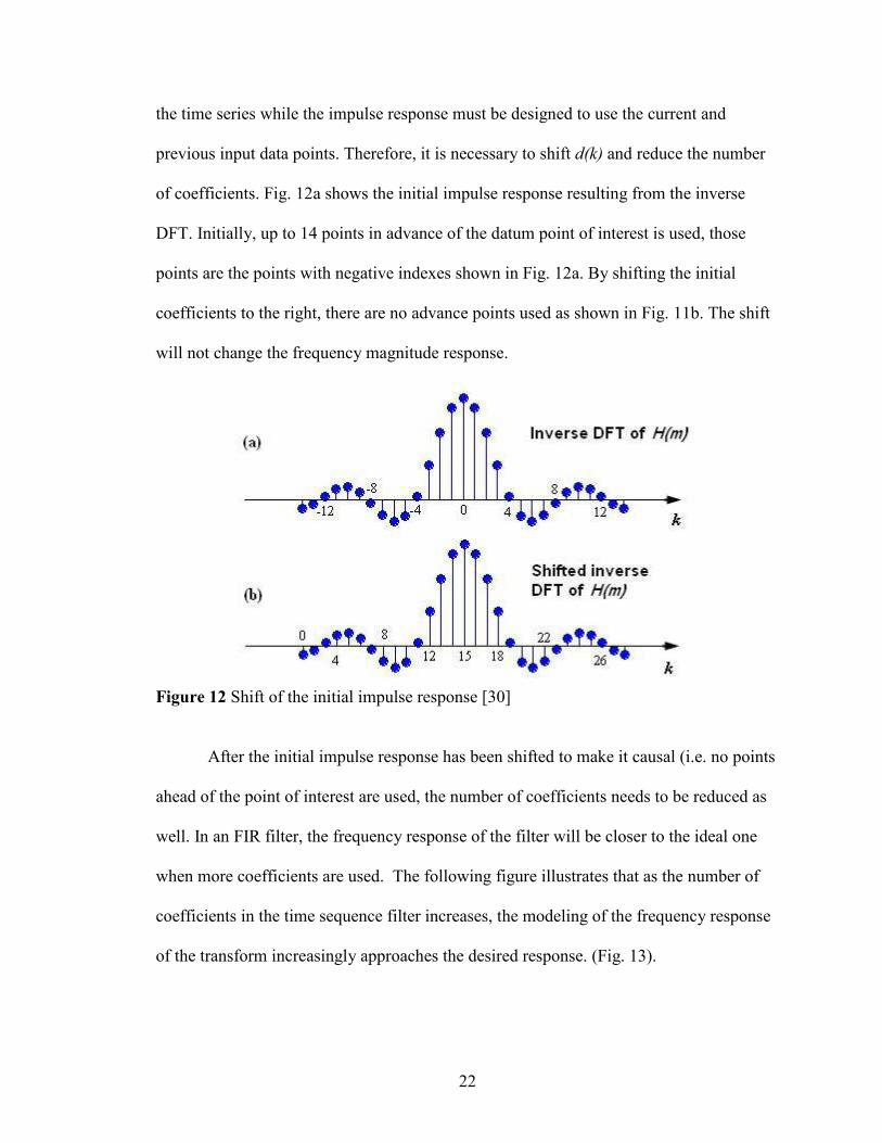
Figure 12 Shift of the initial impulse response [30]
After the initial impulse response has been shifted to make it causal (i.e. no points
ahead of the point of interest are used, the number of coefficients needs to be reduced as
well. In an FIR filter, the frequency response of the filter will be closer to the ideal one
when more coefficients are used. The following figure illustrates that as the number of
coefficients in the time sequence filter increases, the modeling of the frequency response
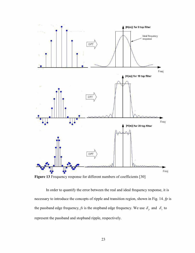
of the transform increasingly approaches the desired response. (Fig. 13).
23
Figure 13 Frequency response for different numbers of coefficients [30]
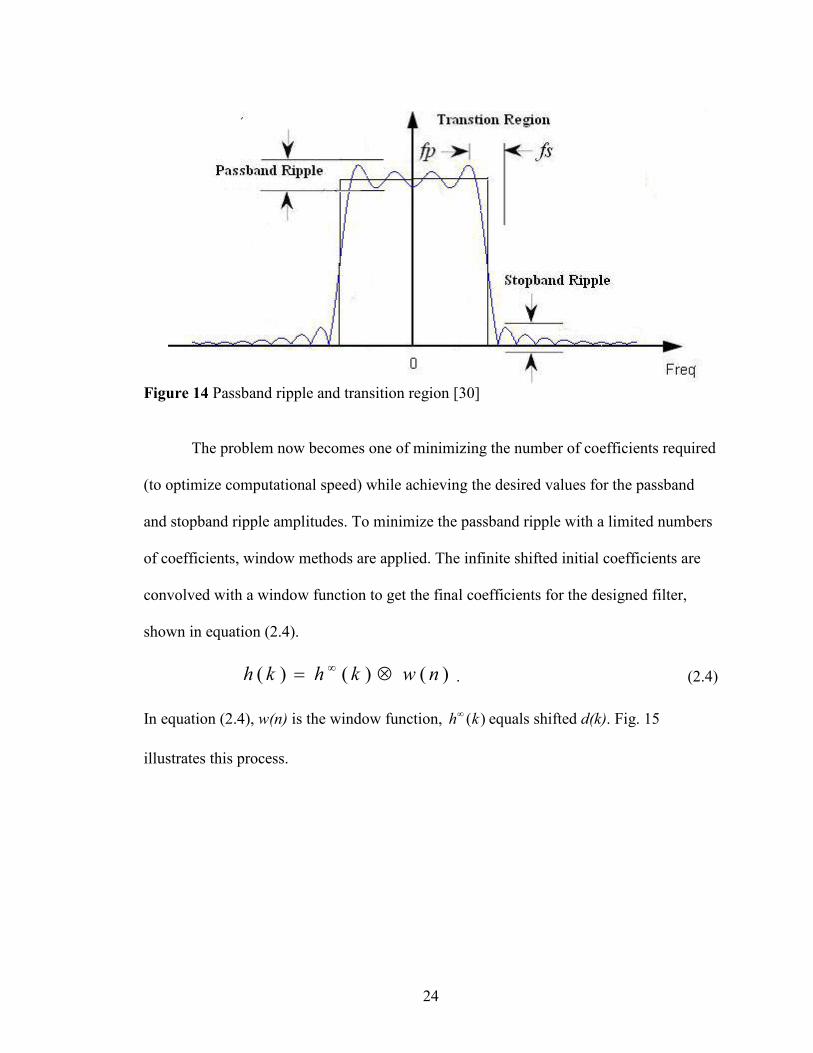
In order to quantify the error between the real and ideal frequency response, it is
necessary to introduce the concepts of ripple and transition region, shown in Fig. 14. fp is
the passband edge frequency, fs is the stopband edge frequency. We use pδ and sδ to
represent the passband and stopband ripple, respectively.
24
Figure 14 Passband ripple and transition region [30]
The problem now becomes one of minimizing the number of coefficients required
(to optimize computational speed) while achieving the desired values for the passband
and stopband ripple amplitudes. To minimize the passband ripple with a limited numbers
of coefficients, window methods are applied. The infinite shifted initial coefficients are
convolved with a window function to get the final coefficients for the designed filter,
shown in equation (2.4).
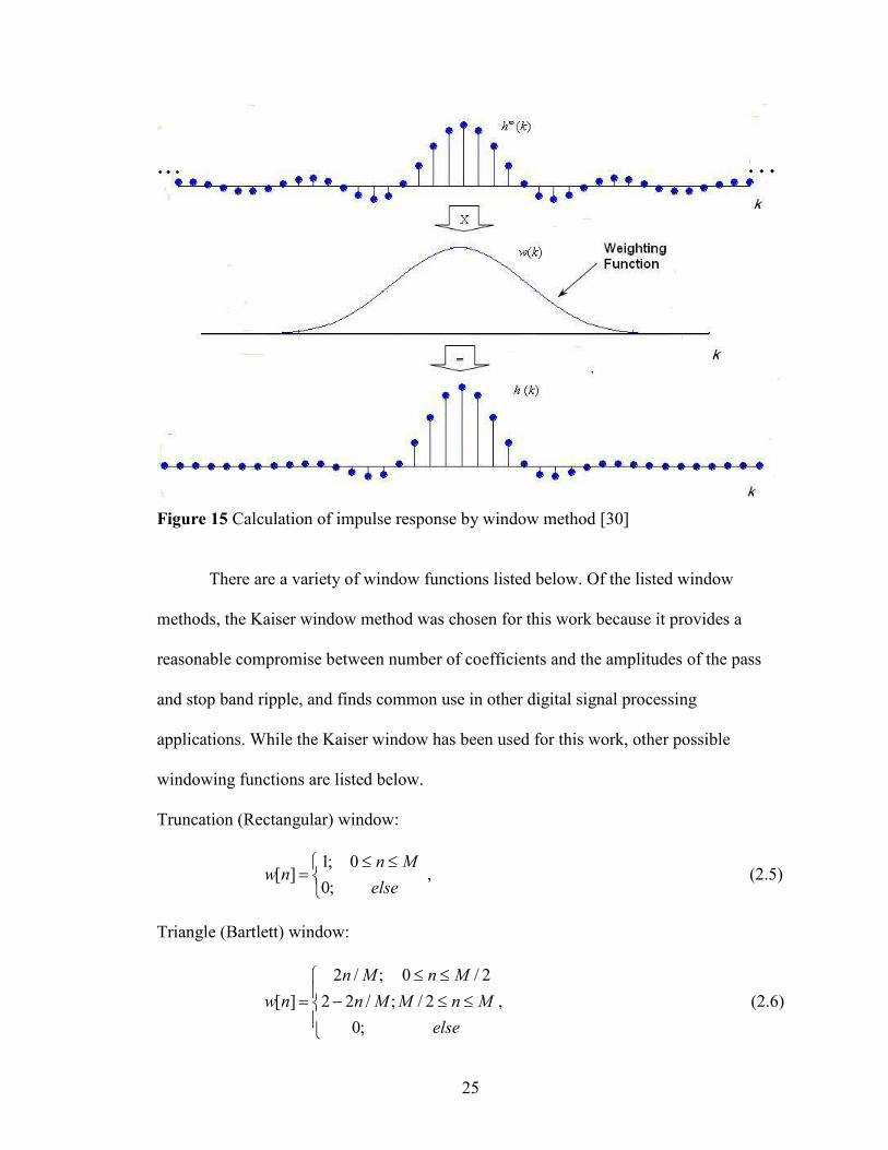
)()()( nwkhkh ⊗= ∞ . (2.4)
In equation (2.4), w(n) is the window function, )(kh∞ equals shifted d(k). Fig. 15
illustrates this process.
25
Figure 15 Calculation of impulse response by window method [30]
There are a variety of window functions listed below. Of the listed window
methods, the Kaiser window method was chosen for this work because it provides a
reasonable compromise between number of coefficients and the amplitudes of the pass
and stop band ripple, and finds common use in other digital signal processing
applications. While the Kaiser window has been used for this work, other possible
windowing functions are listed below.
Truncation (Rectangular) window:
≤≤
=else
Mnnw
;00;1
][ , (2.5)
Triangle (Bartlett) window:
≤≤
≤≤−=
elseMnM
MnMn
Mnnw 2/
2/0
;0;/22
;/2][ , (2.6)
26
Hamming window:
≤≤−
=else
MnMnnw
;00);/2cos(46.054.0
][π
, (2.7)
Hanning window:
≤≤−
=else
MnMnnw
;00);/2cos(5.05.0
][π
, (2.8)
Blackman window:
≤≤+−
=else
MnMnMnnw
;00);/4cos(08.0)/2cos(5.042.0
][ππ
, (2.9)
Kaiser window:
−
≤≤−−
−=
otherwise02
12
1,)(
]1
2[(1][
0
20 NnN
IN
nInw
β
β, (2.10)
where )(0 xI represents the zero order modified Bessel function of the first kind. )(0 xI is
typically evaluated using the following expansion:
2
10 ])2/([1)( ∑
=
+=L
k
k
kxxI , (2.11)
β is estimated from one of the following empirical relationships:
≥<<
−=−+−=
≤=
dBAdBA
AAA
dBAβ
505021dB
)7.8(1102.0)21(07886.0)21(5842.0
2104.0
ββ . (2.12)
In these equations, A is the stopband attenuation and is related to ripple, δ , by
δ10log20−=A , where ),min( sp δδδ = , pδ is the required passband ripple and sδ is the
required stopband ripple. The number of coefficients N can be calculated by
27
fAN
∆−
≥36.14
95.7 , (2.13)
where f∆ is the normalized width for the transition region.
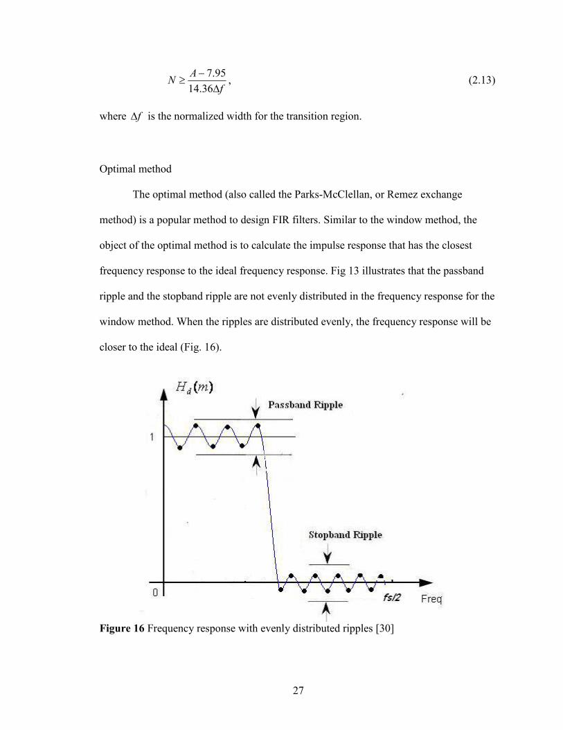
Optimal method
The optimal method (also called the Parks-McClellan, or Remez exchange
method) is a popular method to design FIR filters. Similar to the window method, the
object of the optimal method is to calculate the impulse response that has the closest
frequency response to the ideal frequency response. Fig 13 illustrates that the passband
ripple and the stopband ripple are not evenly distributed in the frequency response for the
window method. When the ripples are distributed evenly, the frequency response will be
closer to the ideal (Fig. 16).
Figure 16 Frequency response with evenly distributed ripples [30]
28
The optimal method equiripples the passband and the stopband in the frequency
response first, and then calculates the coefficients using the equirippled frequency
response. The difference between the ideal frequency response and the designed
frequency response is expressed as:
)]()()[()( ωωωω HHWE D −= . (2.14)
In equation (2.14), )(ωDH is the ideal frequency response, )(ωH is the designed
frequency response, )(ωW is a weighting function and )(ωE is the difference. Rabiner and
Gold [31] found that when the maximum weighted error is minimized, the resulting filter
coefficients will be evenly distributed. Therefore the optimal method finds the impulse
response h(k) that can minimize the maximum weighted error in the passband and the
stopband. For an FIR filter, when the ripples are evenly distributed, the number of
extremal frequencies (marked as black dots in Fig. 16) can be determined by the tap
number of the impulse response. When the extremal frequency is known, it is possible to
determine the frequency response and then calculate the impulse response. It is also
possible to use the Remez exchange algorithm to determine the extremal frequencies
[32]. While the optimal method is presented here for completeness, the results presented
in this work are based on the use of the Kaiser window. It might be expected that results
similar to those shown below would be obtained with the optimal filter, but that is the
subject of further research.
ROC Curve
Receiver operating characteristic (ROC) curves have been widely used in
statistical and medical disciplines [33-36]. The ROC curve is widely used for diagnostic
29
testing to evaluate the effectiveness of different diagnostic methods [34]. In this work, the
ROC curve is used to test the diagnostic result of ECG spectra before and after signal
processing. The ROC curve is a graphical plot of the sensitivity versus one minus
specificity used in a classification test, where the sensitivity and specificity, defined
below, are a measure of the ability of a particular test to discern the presence of a disease
state and then to distinguish this disease state from others, respectively. There are three
types of procedures for evaluating test results in common medical use. They are the
binary test, the continuous test and the ordinal test.
Binary test
The binary test is a basic classification tool in medicine where positive is diseased
and negative is healthy. The object of the test is to separate the population into two
subsets, healthy and diseased. Sensitivity (SN) and specificity (SP) are commonly used to
describe the accuracy of the particular test. SN and SP are calculated according to
equations (2.15) and (2.16).
FNTPTPSN+
= , (2.15)
FPTNTNSP+
= . (2.16)
In equation (2.15) and (2.16) TP, TN, FP, FN stand for true positive, true negative, false
positive and false negative respectively. If the subject is positive (disease present), and
the test specifies the subject as positive, this is called a ‘true positive’. False positive
indicates that the subject that is negative (disease absent) is mistakenly classified as
positive. Therefore, from the above equations it is apparent that sensitivity depends on
30
correctly identifying positive subjects while specificity depends on correctly
discriminating against negative subjects. The binary test is therefore a popular measure of
test accuracy.
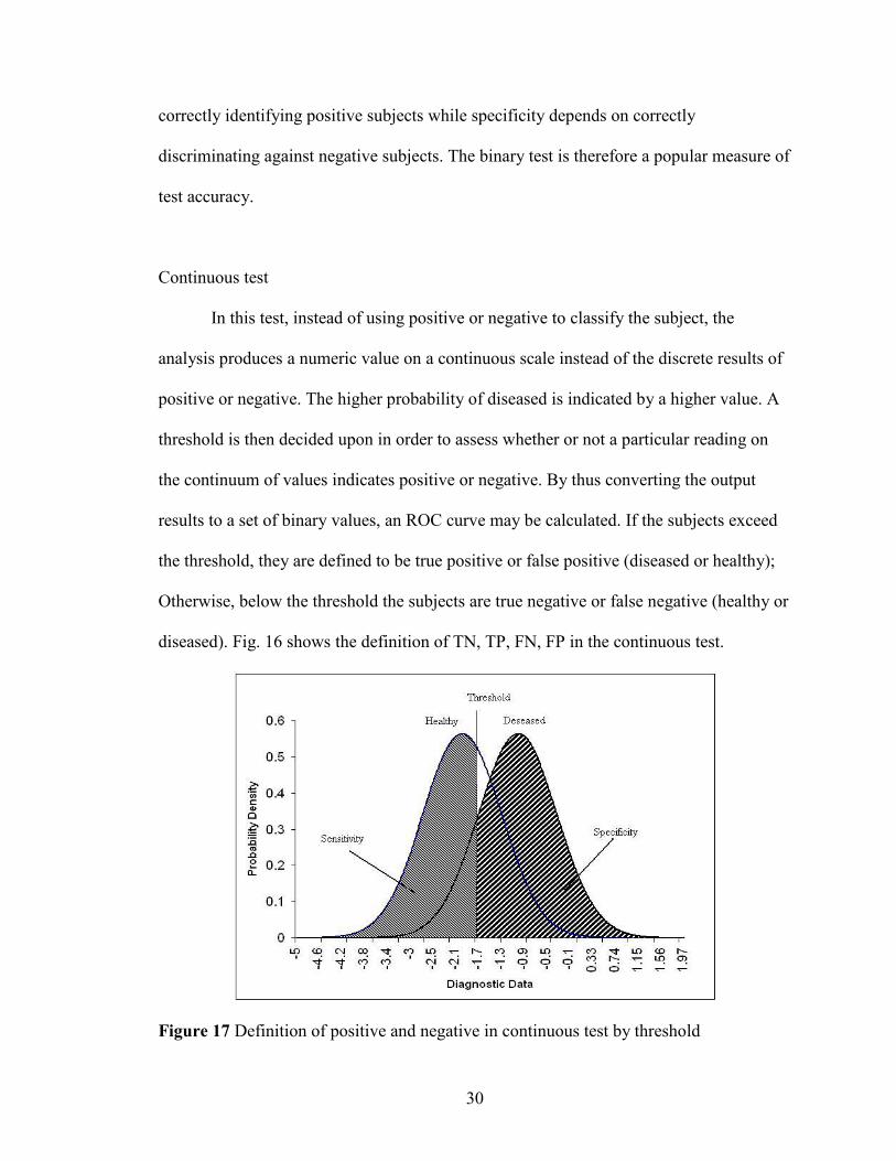
Continuous test
In this test, instead of using positive or negative to classify the subject, the
analysis produces a numeric value on a continuous scale instead of the discrete results of
positive or negative. The higher probability of diseased is indicated by a higher value. A
threshold is then decided upon in order to assess whether or not a particular reading on
the continuum of values indicates positive or negative. By thus converting the output
results to a set of binary values, an ROC curve may be calculated. If the subjects exceed
the threshold, they are defined to be true positive or false positive (diseased or healthy);
Otherwise, below the threshold the subjects are true negative or false negative (healthy or
diseased). Fig. 16 shows the definition of TN, TP, FN, FP in the continuous test.
Figure 17 Definition of positive and negative in continuous test by threshold
31
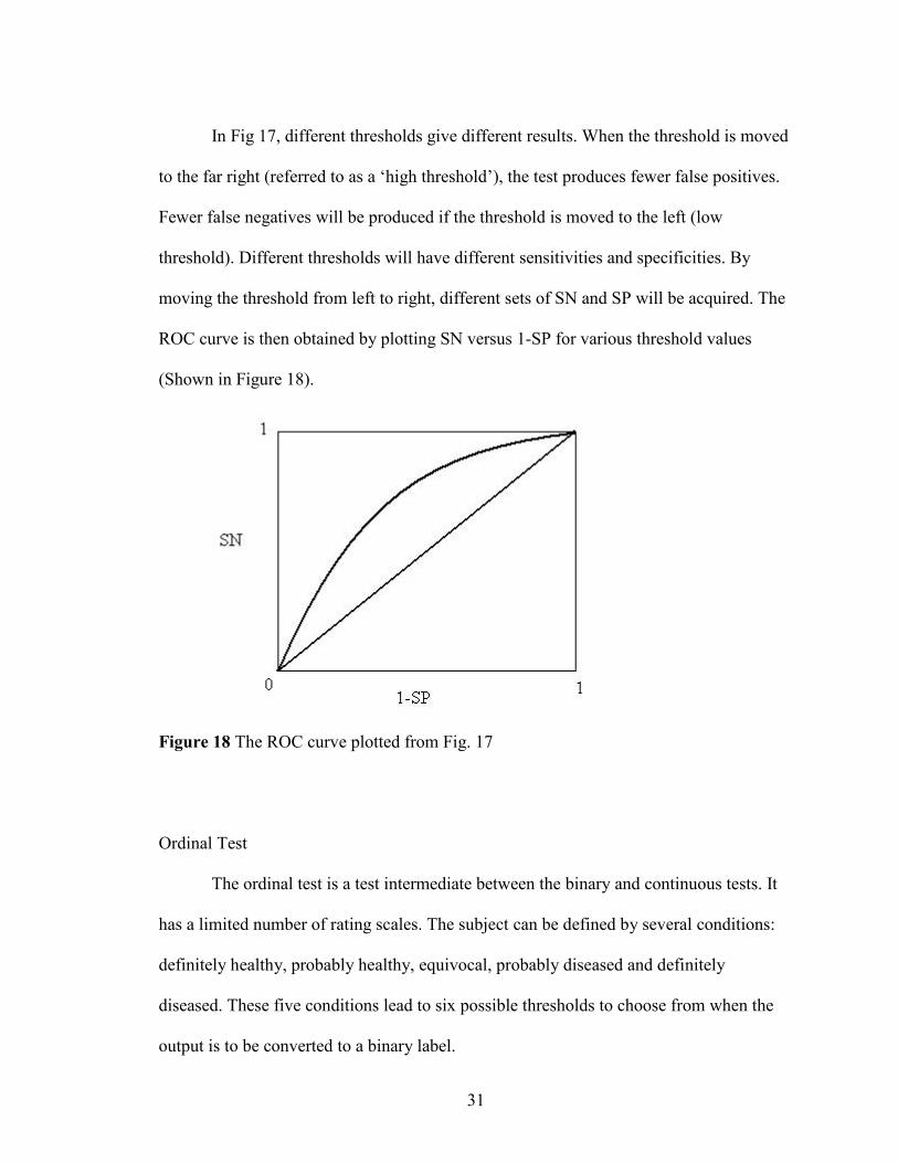
In Fig 17, different thresholds give different results. When the threshold is moved
to the far right (referred to as a ‘high threshold’), the test produces fewer false positives.
Fewer false negatives will be produced if the threshold is moved to the left (low
threshold). Different thresholds will have different sensitivities and specificities. By
moving the threshold from left to right, different sets of SN and SP will be acquired. The
ROC curve is then obtained by plotting SN versus 1-SP for various threshold values
(Shown in Figure 18).
Figure 18 The ROC curve plotted from Fig. 17
Ordinal Test
The ordinal test is a test intermediate between the binary and continuous tests. It
has a limited number of rating scales. The subject can be defined by several conditions:
definitely healthy, probably healthy, equivocal, probably diseased and definitely
diseased. These five conditions lead to six possible thresholds to choose from when the
output is to be converted to a binary label.
32
Calculation and Graphing of ROC Values
To show how an ROC curve is obtained from a binary test, several publicly
available ECG spectra have been analyzed and the ST segment elevations calculated. ST
segment elevations of the ECG spectrum can be used as an indicator of myocardial
infraction. Fortunately, these publicly available data [3] also contain the clinical
diagnosis of the patient. The diagnosis of the patient is either healthy or suffering
myocardial infarction. Therefore, this is a binary test. In Table 1, the ST segment
elevations are calculated from the ECG spectra of two groups of people. The
measurement of ST segment elevation is addressed in Chapter III. One group is the
control group while the other is known to have suffered myocardial infarction. The ST
segments of the two groups are separated in columns and sorted in ascending order for
the amplitude of the ST segment elevation.
The ROC curve plots SN versus 1-SP as the threshold varies across the entire
range [38]. Each threshold defines a specific set of TP, TN, FP, FN, from which SN and
SP can be calculated by equations (2.15) and (2.16).
To obtain the ROC curve from Table 1, a horizontal threshold between each row
is defined. The threshold starts from the top of the first row, moving between the rows
until the bottom of the last row is reached. The rows below the threshold are defined as
positives for the test, while the rows above are negative. True positive (TP) is the count
of healthy people below the threshold. True negative (TN) is the count of people who
have suffered myocardial infraction above the threshold. False positive (FP) equals the
33
total number of healthy people less true negatives (TN). False negative (FN) is the total
number of diseased people less true positives (TP). Table 1 shows the calculation of each
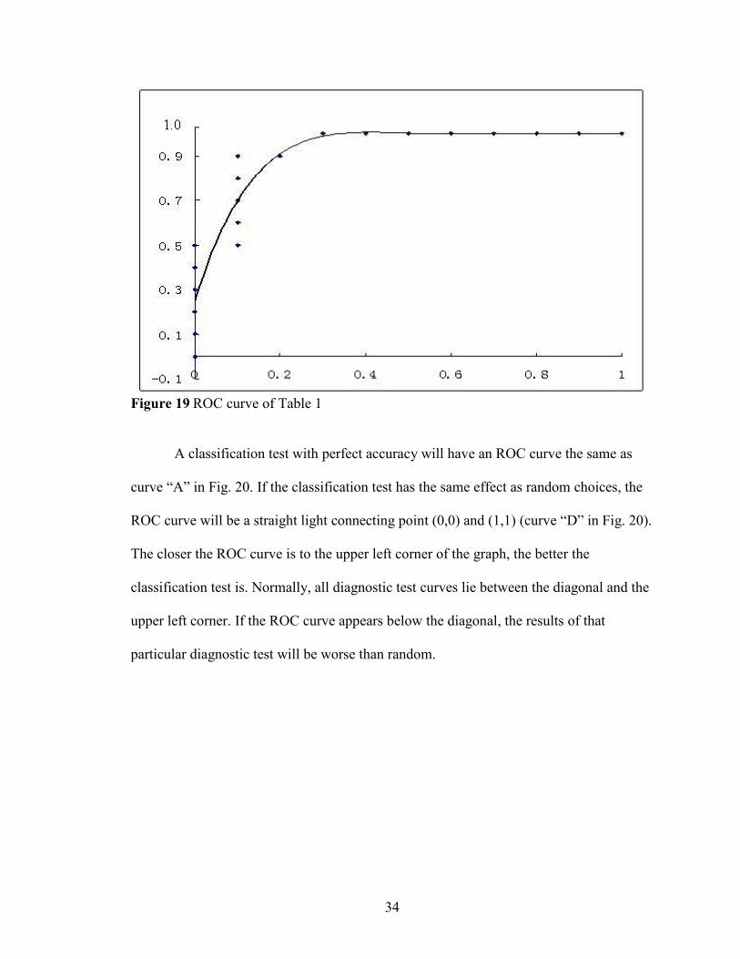
parameter. SN versus 1-SP, this data is then being plotted in Fig. 19. Figure 19 shows that
for this sample of data, the ROC curve indicates a reasonably accurate diagnostic test as
indicated by the area under the ROC curve compared with a random threshold line.
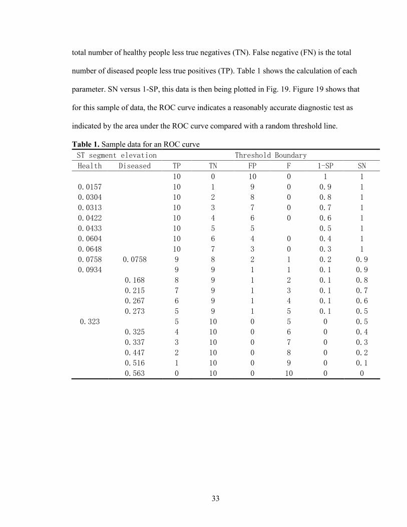
Table 1. Sample data for an ROC curve ST segment elevation Threshold Boundary
Health Diseased TP TN FP F 1-SP SN
10 0 10 0 1 1
0.0157 10 1 9 0 0.9 1
0.0304 10 2 8 0 0.8 1
0.0313 10 3 7 0 0.7 1
0.0422 10 4 6 0 0.6 1
0.0433 10 5 5 0.5 1
0.0604 10 6 4 0 0.4 1
0.0648 10 7 3 0 0.3 1
0.0758 0.0758 9 8 2 1 0.2 0.9
0.0934 9 9 1 1 0.1 0.9
0.168 8 9 1 2 0.1 0.8
0.215 7 9 1 3 0.1 0.7
0.267 6 9 1 4 0.1 0.6
0.273 5 9 1 5 0.1 0.5
0.323 5 10 0 5 0 0.5
0.325 4 10 0 6 0 0.4
0.337 3 10 0 7 0 0.3
0.447 2 10 0 8 0 0.2
0.516 1 10 0 9 0 0.1
0.563 0 10 0 10 0 0
34
Figure 19 ROC curve of Table 1
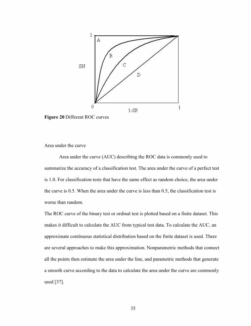
A classification test with perfect accuracy will have an ROC curve the same as
curve “A” in Fig. 20. If the classification test has the same effect as random choices, the
ROC curve will be a straight light connecting point (0,0) and (1,1) (curve “D” in Fig. 20).
The closer the ROC curve is to the upper left corner of the graph, the better the
classification test is. Normally, all diagnostic test curves lie between the diagonal and the
upper left corner. If the ROC curve appears below the diagonal, the results of that
particular diagnostic test will be worse than random.
35
Figure 20 Different ROC curves
Area under the curve
Area under the curve (AUC) describing the ROC data is commonly used to
summarize the accuracy of a classification test. The area under the curve of a perfect test
is 1.0. For classification tests that have the same effect as random choice, the area under
the curve is 0.5. When the area under the curve is less than 0.5, the classification test is
worse than random.
The ROC curve of the binary test or ordinal test is plotted based on a finite dataset. This
makes it difficult to calculate the AUC from typical test data. To calculate the AUC, an
approximate continuous statistical distribution based on the finite dataset is used. There
are several approaches to make this approximation. Nonparametric methods that connect
all the points then estimate the area under the line, and parametric methods that generate
a smooth curve according to the data to calculate the area under the curve are commonly
used [37].

36
Partial area under the curve
Although the area under the curve is the most popular variable to parameterize the
ROC curve, it may not be useful in some situations. Different ROC curves may have the
same AUC. For some tests, only the test value above certain specificities is useful. In
these situations, the AUC for the entire scale is not applicable. To calculate the partial
area under the curve, both parametric and nonparametric methods can be applied [39,
40].In the parametric method, the points above the required specificity are linked to
estimate the partial area under the curve. The nonparametric method estimates a curve for
the points and uses the area under the estimated curve as the result.
37
CHAPTER III
RESULTS AND DISCUSSION
For the results reported below, ECG spectra from the PTB diagnostic database [3]
are used for signal processing, feature extraction and classification test.
PTB diagnostic database
The ECG spectra in the PTB diagnostic database were obtained using a non-
commercial, PTB prototype recorder with the following specifications:
1. 16 input channels, (14 for ECGs, 1 for respiration, 1 for line voltage)
2. Input voltage: ±16 mV, compensated offset voltage up to ± 300 mV
3. Input resistance: 100 Ω (DC)
4. Resolution: 16 bit with 0.5 µV/LSB (2000 A/D units per mV)
5. Bandwidth: 0 - 1 kHz (synchronous sampling of all channels)
6. Noise voltage: max. 10 µV (pp), respectively 3 µV (RMS) with input short circuit
7. Online recording of skin resistance
8. Noise level recording during signal collection
The database contains 549 records from 294 subjects (each subject is represented
by one to five records). Each record includes 15 simultaneously measured signals: the
conventional 12 leads (i, ii, iii, avr, avl, avf, v1, v2, v3, v4, v5, v6) together with the 3
38
Frank lead ECGs (vx, vy, vz). Each signal is digitized at 1000 samples per second, with
16 bit resolution over a range of ± 16.384 mV.
Table 2. Content for PTB diagnostic database
Diagnostic class Number of subjectsMyocardial infarction 148Cardiomyopathy/Heart failure 18Bundle branch block 15Dysrhythmia 14Myocardial hypertrophy 7Valvular heart disease 6Myocarditis 4Miscellaneous 5Healthy controls 54
Signal Processing and results
Data smoothing and results
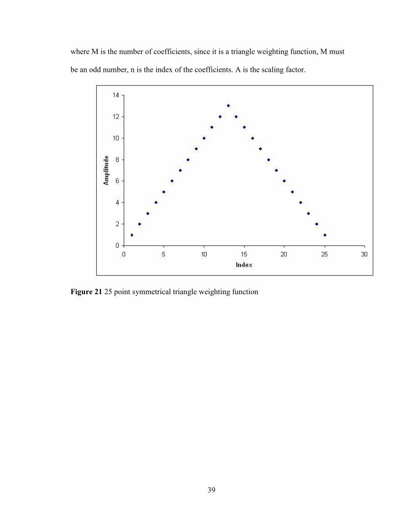
To determine which function to use for ECG spectral smoothing, a 25 point
symmetrical weighting function (ST smooth, Fig. 21) and a 25 Savitzky Golay smooth
(Fig 22) are applied to the ECG signal. The impulse response of Savitzky-Golay smooth
is shown in [28]. The coefficients and scaling factor of the symmetrical triangle weighing
function used in this paper can be calculated using equations 3.1 and 3.2. The coefficients
calculated are shown in appendix.
≤≤+
+≤≤
+−=
else
MnM
Mn
nMn
nh2
32
11
;0;1
;][ , (3.1)
2)2
1( +=
MA , (3.2)
39
where M is the number of coefficients, since it is a triangle weighting function, M must
be an odd number, n is the index of the coefficients. A is the scaling factor.
Figure 21 25 point symmetrical triangle weighting function
40
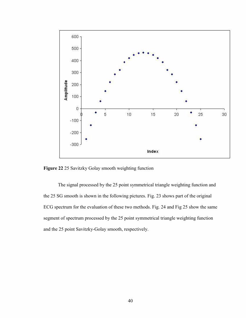
Figure 22 25 Savitzky Golay smooth weighting function
The signal processed by the 25 point symmetrical triangle weighting function and
the 25 SG smooth is shown in the following pictures. Fig. 23 shows part of the original
ECG spectrum for the evaluation of these two methods. Fig. 24 and Fig 25 show the same
segment of spectrum processed by the 25 point symmetrical triangle weighting function
and the 25 point Savitzky-Golay smooth, respectively.
41
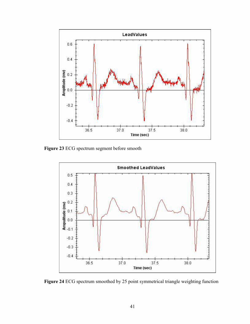
Figure 23 ECG spectrum segment before smooth
Figure 24 ECG spectrum smoothed by 25 point symmetrical triangle weighting function
42
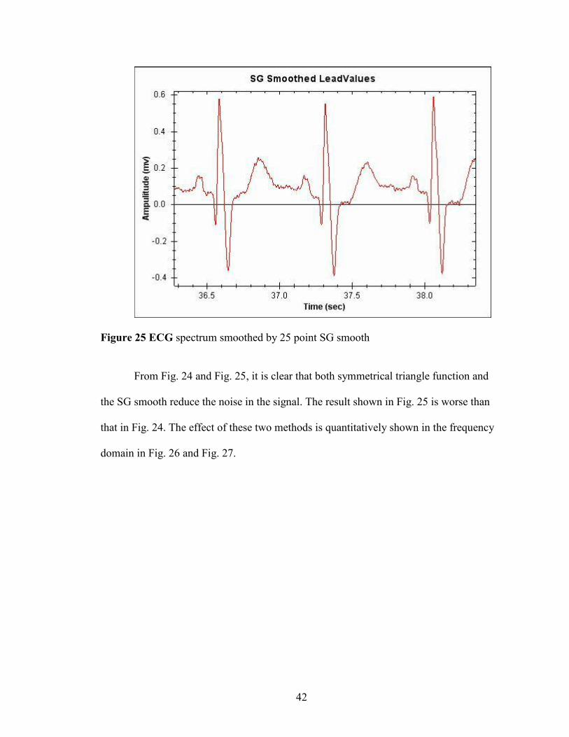
Figure 25 ECG spectrum smoothed by 25 point SG smooth
From Fig. 24 and Fig. 25, it is clear that both symmetrical triangle function and
the SG smooth reduce the noise in the signal. The result shown in Fig. 25 is worse than
that in Fig. 24. The effect of these two methods is quantitatively shown in the frequency
domain in Fig. 26 and Fig. 27.
43
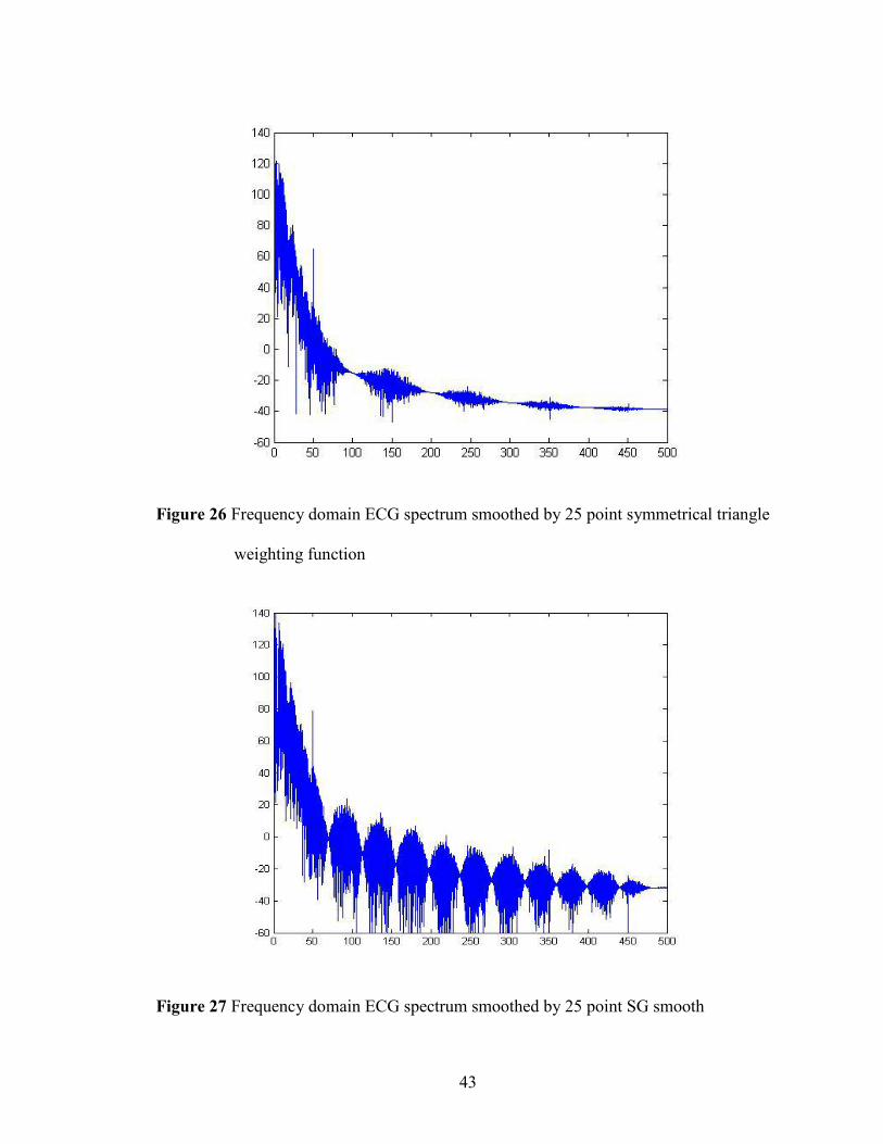
Figure 26 Frequency domain ECG spectrum smoothed by 25 point symmetrical triangle
weighting function
Figure 27 Frequency domain ECG spectrum smoothed by 25 point SG smooth
44
By comparing Fig. 26 and Fig. 27, it can be concluded that the triangle
symmetrical weighting function increases noise reduction compared with the application
of the same number of coefficients via an SG smooth. Therefore, the symmetrical triangle
weighting function is more efficient compared to the SG smooth in ECG spectra. The
symmetrical triangle weighting function has been used in this work to reduce the high
frequency noise in ECG spectra.
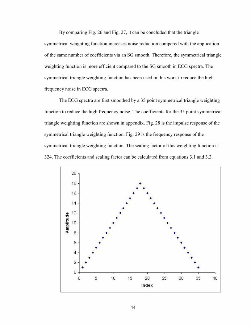
The ECG spectra are first smoothed by a 35 point symmetrical triangle weighting
function to reduce the high frequency noise. The coefficients for the 35 point symmetrical
triangle weighting function are shown in appendix. Fig. 28 is the impulse response of the
symmetrical triangle weighting function. Fig. 29 is the frequency response of the
symmetrical triangle weighting function. The scaling factor of this weighting function is
324. The coefficients and scaling factor can be calculated from equations 3.1 and 3.2.
45
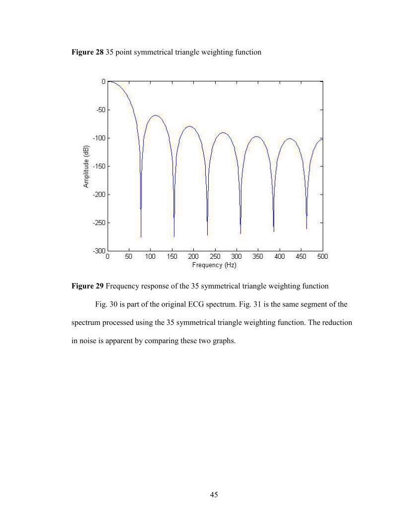
Figure 28 35 point symmetrical triangle weighting function
Figure 29 Frequency response of the 35 symmetrical triangle weighting function
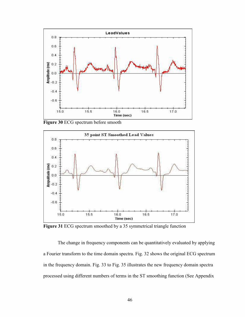
Fig. 30 is part of the original ECG spectrum. Fig. 31 is the same segment of the
spectrum processed using the 35 symmetrical triangle weighting function. The reduction
in noise is apparent by comparing these two graphs.
46
Figure 30 ECG spectrum before smooth
Figure 31 ECG spectrum smoothed by a 35 symmetrical triangle function
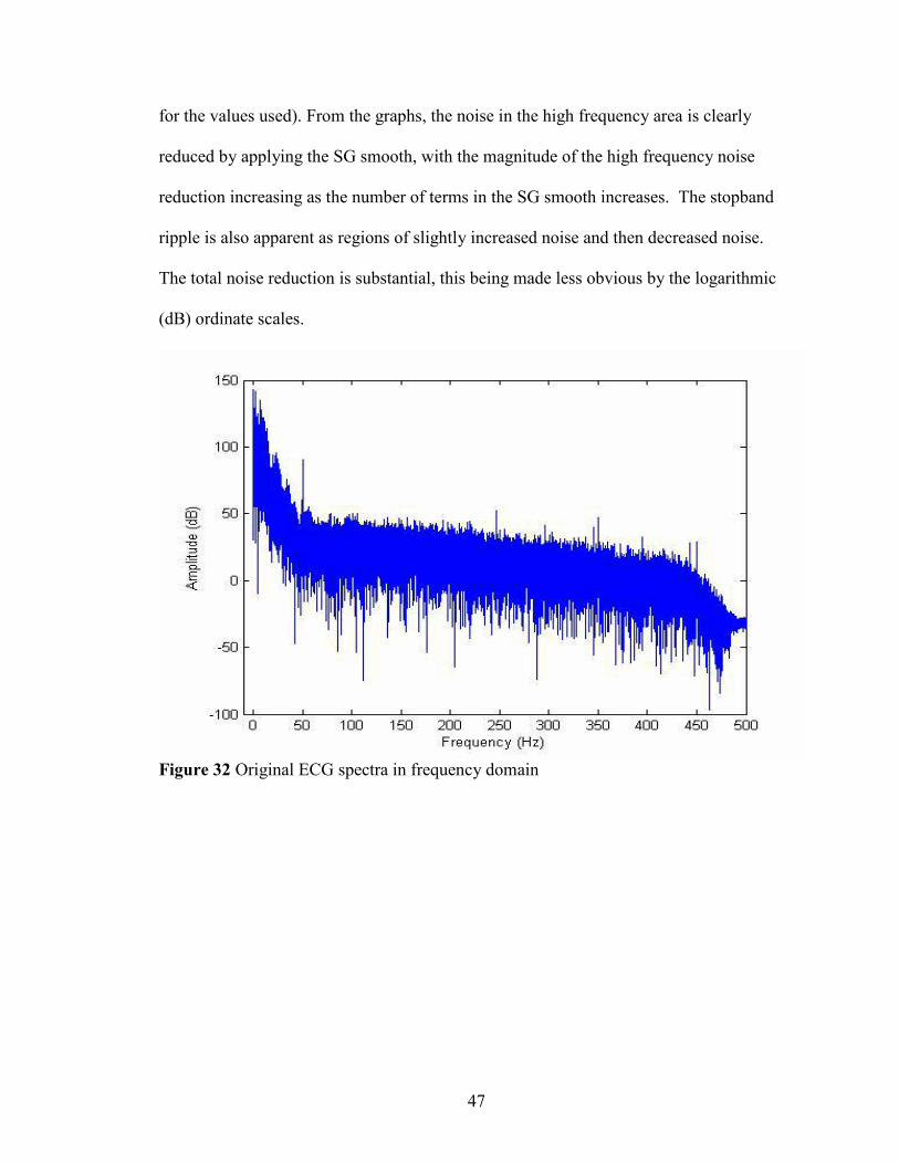
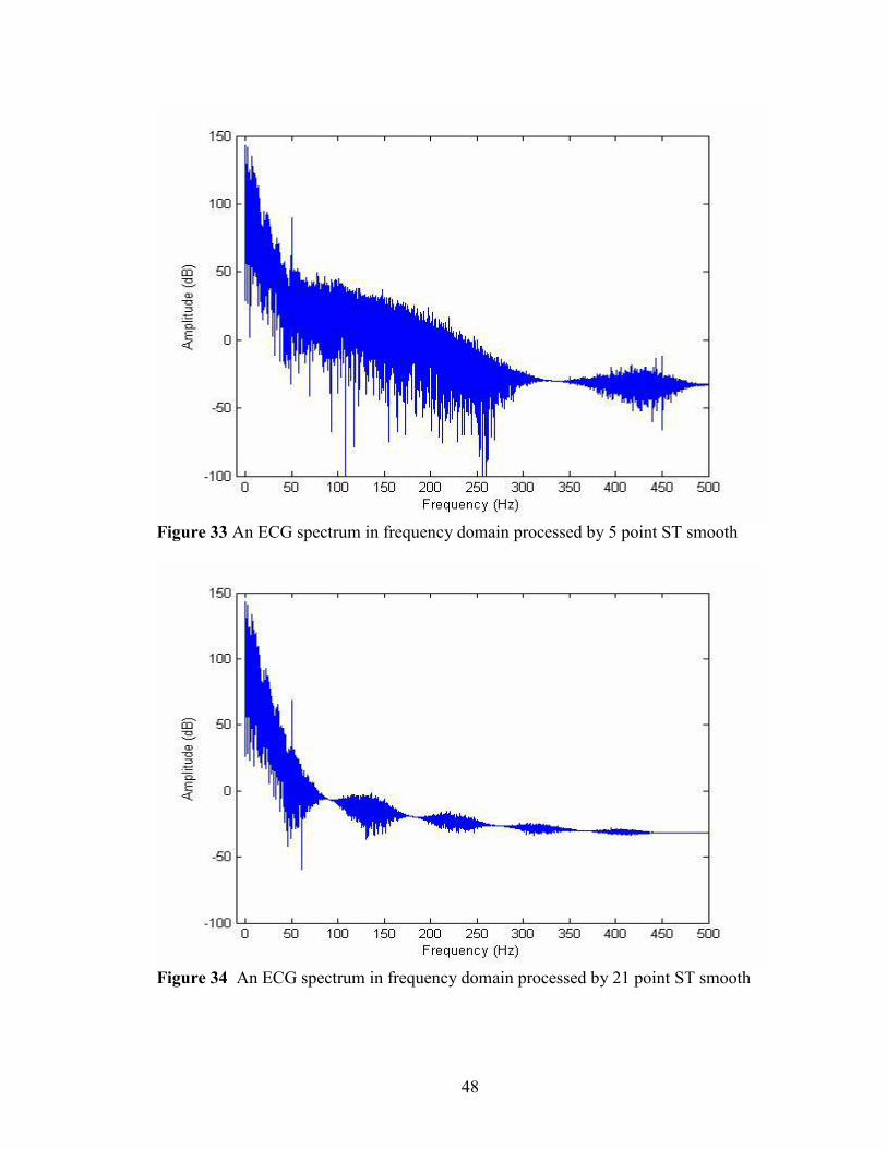
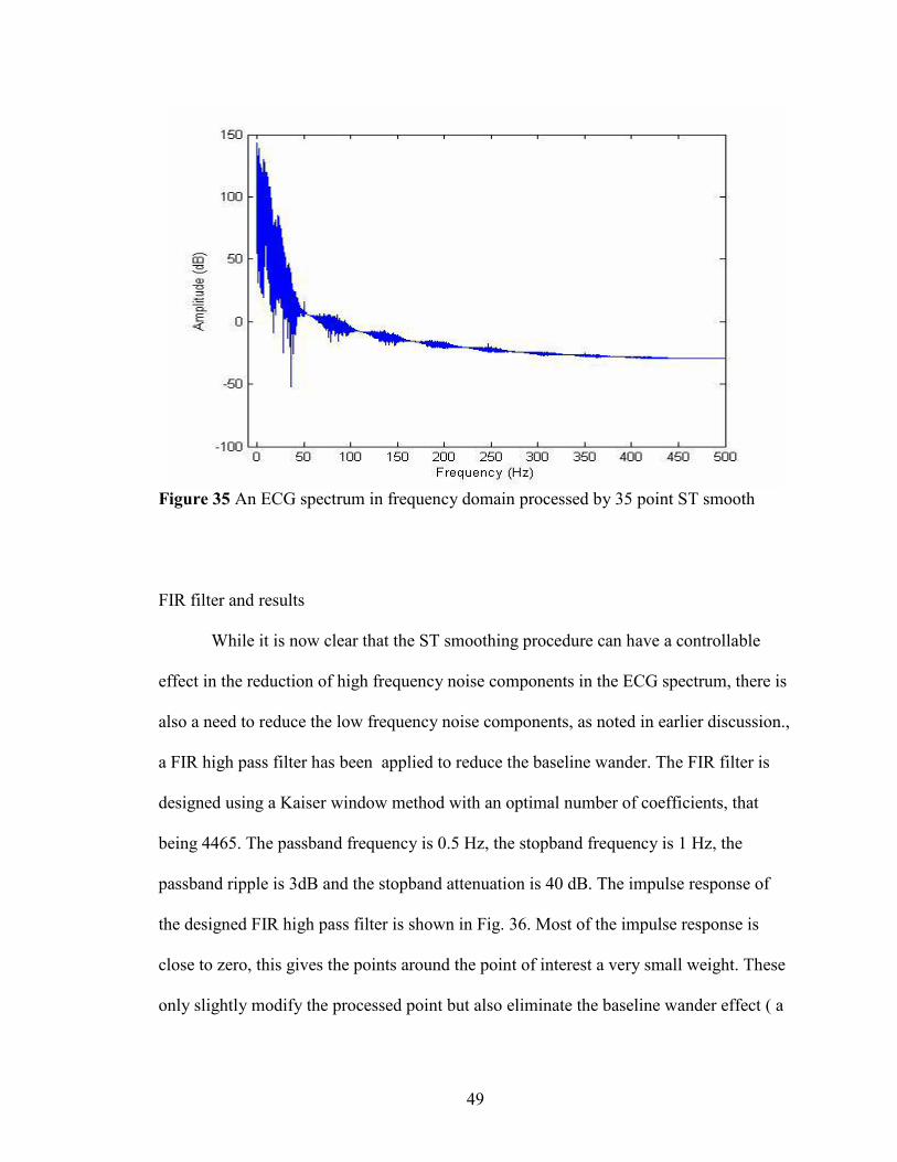
The change in frequency components can be quantitatively evaluated by applying
a Fourier transform to the time domain spectra. Fig. 32 shows the original ECG spectrum
in the frequency domain. Fig. 33 to Fig. 35 illustrates the new frequency domain spectra
processed using different numbers of terms in the ST smoothing function (See Appendix
47
for the values used). From the graphs, the noise in the high frequency area is clearly
reduced by applying the SG smooth, with the magnitude of the high frequency noise
reduction increasing as the number of terms in the SG smooth increases. The stopband
ripple is also apparent as regions of slightly increased noise and then decreased noise.
The total noise reduction is substantial, this being made less obvious by the logarithmic
(dB) ordinate scales.
Figure 32 Original ECG spectra in frequency domain
48
Figure 33 An ECG spectrum in frequency domain processed by 5 point ST smooth
Figure 34 An ECG spectrum in frequency domain processed by 21 point ST smooth
49
Figure 35 An ECG spectrum in frequency domain processed by 35 point ST smooth
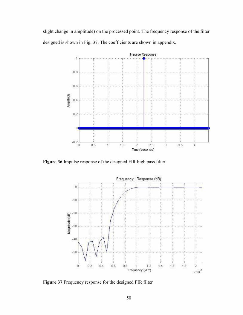
FIR filter and results
While it is now clear that the ST smoothing procedure can have a controllable
effect in the reduction of high frequency noise components in the ECG spectrum, there is
also a need to reduce the low frequency noise components, as noted in earlier discussion.,
a FIR high pass filter has been applied to reduce the baseline wander. The FIR filter is
designed using a Kaiser window method with an optimal number of coefficients, that
being 4465. The passband frequency is 0.5 Hz, the stopband frequency is 1 Hz, the
passband ripple is 3dB and the stopband attenuation is 40 dB. The impulse response of
the designed FIR high pass filter is shown in Fig. 36. Most of the impulse response is
close to zero, this gives the points around the point of interest a very small weight. These
only slightly modify the processed point but also eliminate the baseline wander effect ( a
50
slight change in amplitude) on the processed point. The frequency response of the filter
designed is shown in Fig. 37. The coefficients are shown in appendix.
Figure 36 Impulse response of the designed FIR high pass filter
Figure 37 Frequency response for the designed FIR filter
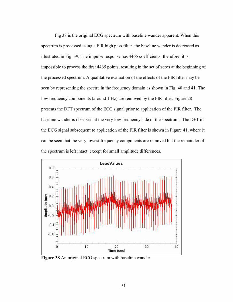
51
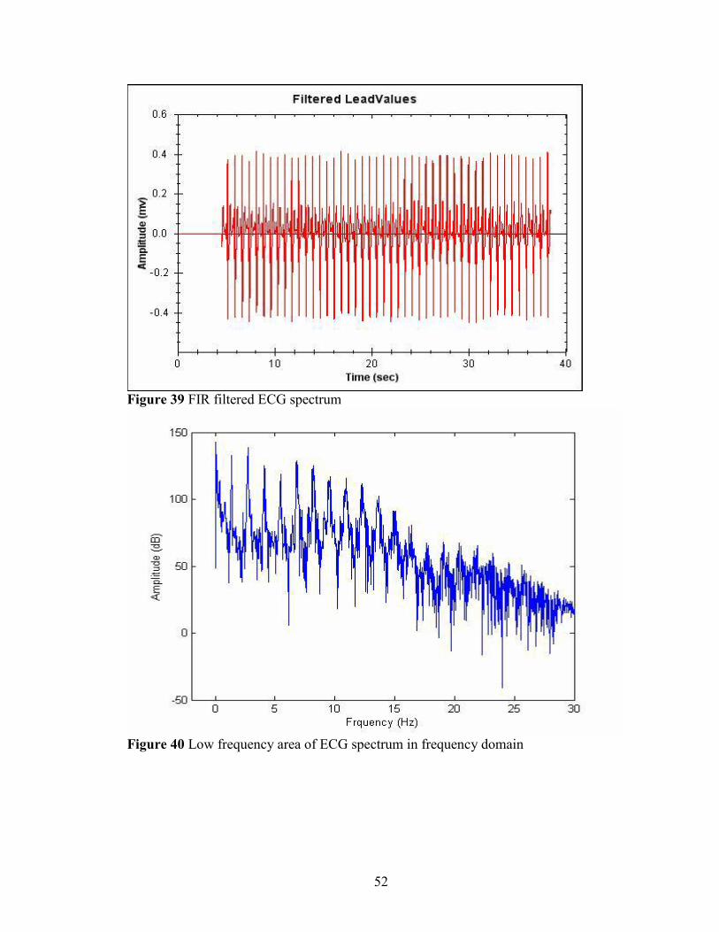
Fig 38 is the original ECG spectrum with baseline wander apparent. When this
spectrum is processed using a FIR high pass filter, the baseline wander is decreased as
illustrated in Fig. 39. The impulse response has 4465 coefficients; therefore, it is
impossible to process the first 4465 points, resulting in the set of zeros at the beginning of
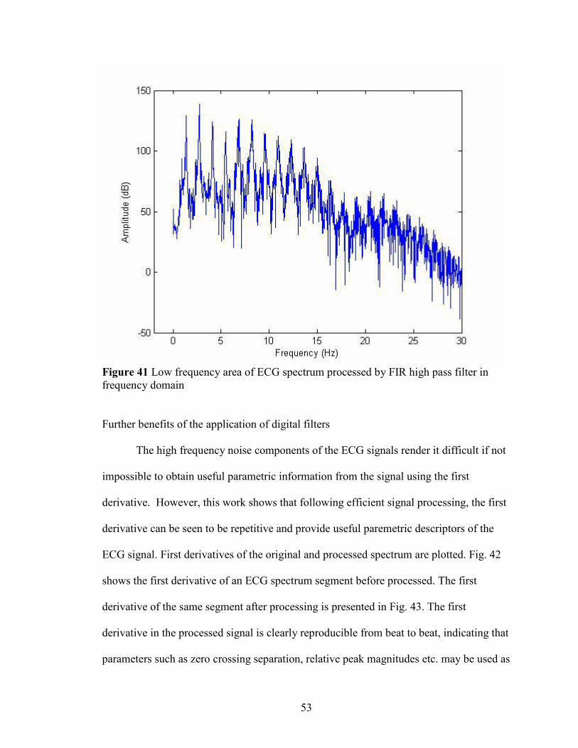
the processed spectrum. A qualitative evaluation of the effects of the FIR filter may be
seen by representing the spectra in the frequency domain as shown in Fig. 40 and 41. The
low frequency components (around 1 Hz) are removed by the FIR filter. Figure 28
presents the DFT spectrum of the ECG signal prior to application of the FIR filter. The
baseline wander is observed at the very low frequency side of the spectrum. The DFT of
the ECG signal subsequent to application of the FIR filter is shown in Figure 41, where it
can be seen that the very lowest frequency components are removed but the remainder of
the spectrum is left intact, except for small amplitude differences.
Figure 38 An original ECG spectrum with baseline wander
52
Figure 39 FIR filtered ECG spectrum
Figure 40 Low frequency area of ECG spectrum in frequency domain
53
Figure 41 Low frequency area of ECG spectrum processed by FIR high pass filter in frequency domain
Further benefits of the application of digital filters
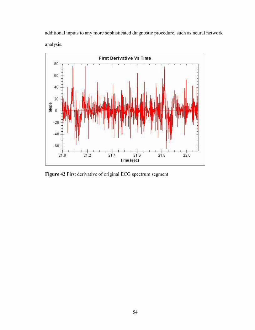
The high frequency noise components of the ECG signals render it difficult if not
impossible to obtain useful parametric information from the signal using the first
derivative. However, this work shows that following efficient signal processing, the first
derivative can be seen to be repetitive and provide useful paremetric descriptors of the
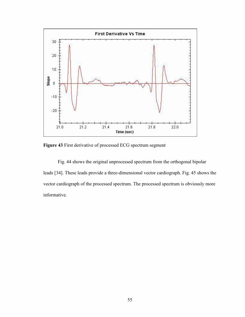
ECG signal. First derivatives of the original and processed spectrum are plotted. Fig. 42
shows the first derivative of an ECG spectrum segment before processed. The first
derivative of the same segment after processing is presented in Fig. 43. The first
derivative in the processed signal is clearly reproducible from beat to beat, indicating that
parameters such as zero crossing separation, relative peak magnitudes etc. may be used as
54
additional inputs to any more sophisticated diagnostic procedure, such as neural network
analysis.
Figure 42 First derivative of original ECG spectrum segment
55
Figure 43 First derivative of processed ECG spectrum segment
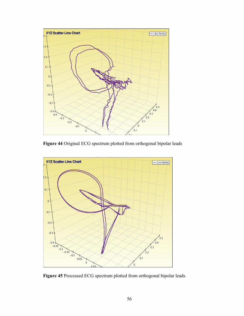
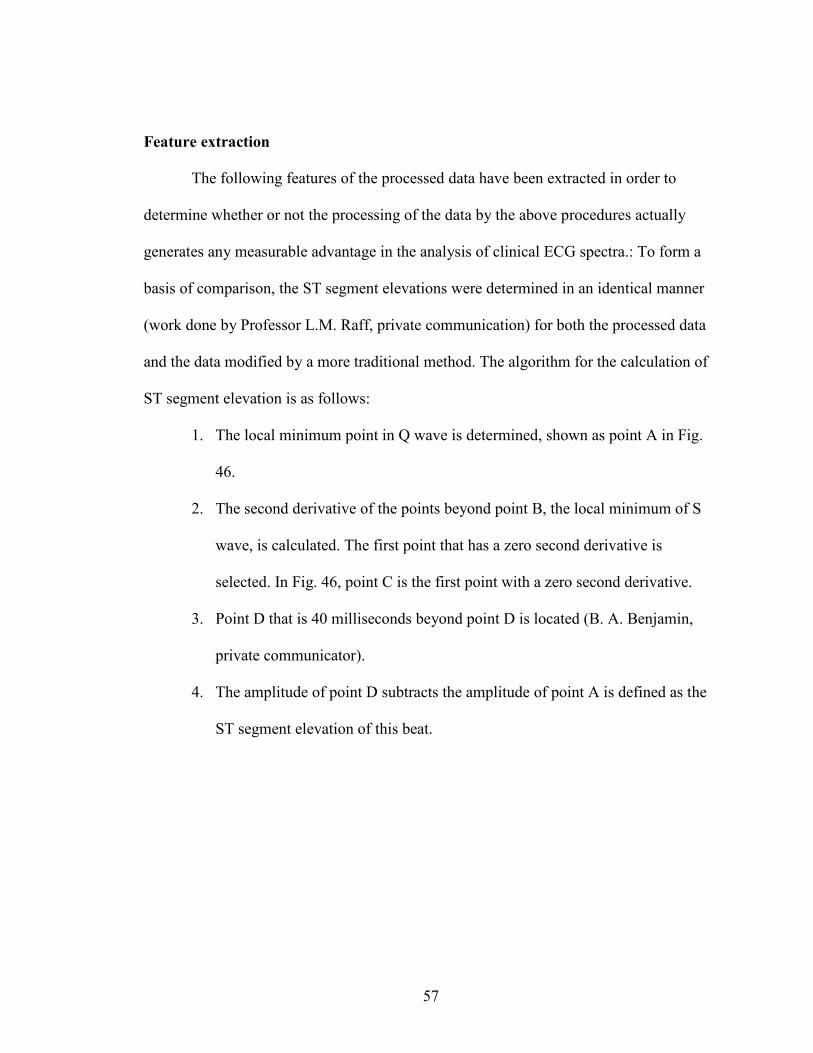
Fig. 44 shows the original unprocessed spectrum from the orthogonal bipolar
leads [34]. These leads provide a three-dimensional vector cardiograph. Fig. 45 shows the
vector cardiograph of the processed spectrum. The processed spectrum is obviously more
informative.
56
Figure 44 Original ECG spectrum plotted from orthogonal bipolar leads
Figure 45 Processed ECG spectrum plotted from orthogonal bipolar leads
57
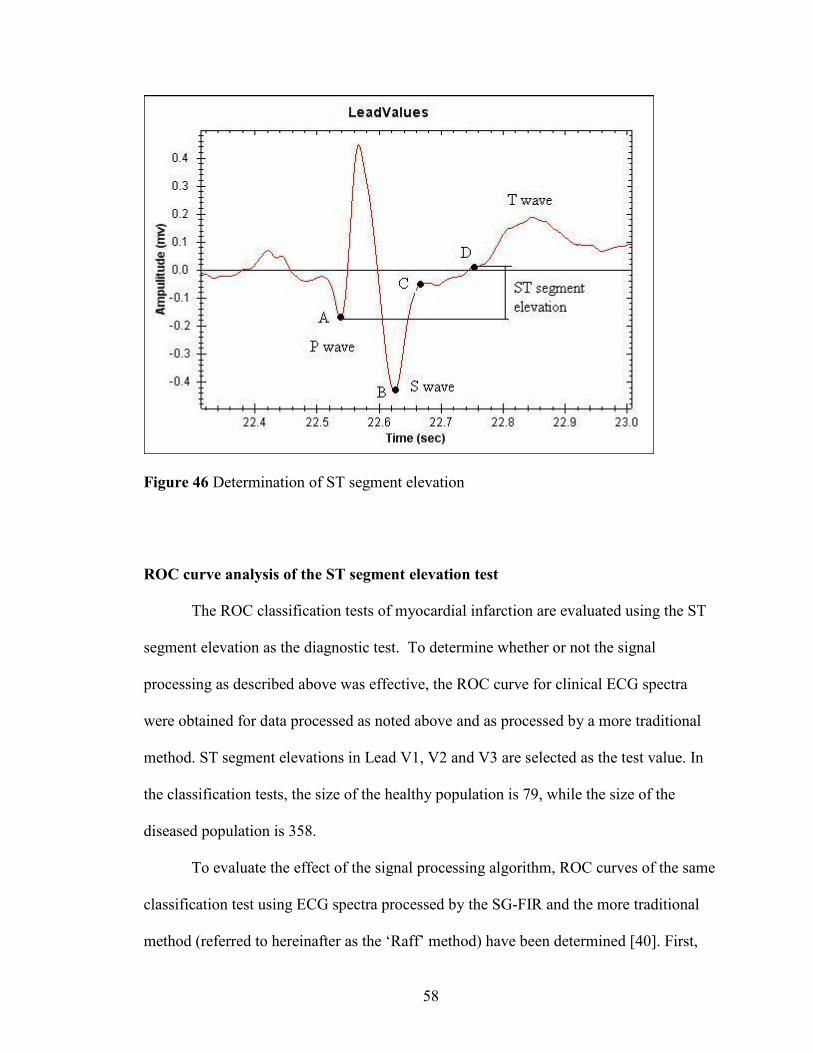
Feature extraction
The following features of the processed data have been extracted in order to
determine whether or not the processing of the data by the above procedures actually
generates any measurable advantage in the analysis of clinical ECG spectra.: To form a
basis of comparison, the ST segment elevations were determined in an identical manner
(work done by Professor L.M. Raff, private communication) for both the processed data
and the data modified by a more traditional method. The algorithm for the calculation of
ST segment elevation is as follows:
1. The local minimum point in Q wave is determined, shown as point A in Fig.
46.
2. The second derivative of the points beyond point B, the local minimum of S
wave, is calculated. The first point that has a zero second derivative is
selected. In Fig. 46, point C is the first point with a zero second derivative.
3. Point D that is 40 milliseconds beyond point D is located (B. A. Benjamin,
private communicator).
4. The amplitude of point D subtracts the amplitude of point A is defined as the
ST segment elevation of this beat.
58
Figure 46 Determination of ST segment elevation
ROC curve analysis of the ST segment elevation test
The ROC classification tests of myocardial infarction are evaluated using the ST
segment elevation as the diagnostic test. To determine whether or not the signal
processing as described above was effective, the ROC curve for clinical ECG spectra
were obtained for data processed as noted above and as processed by a more traditional
method. ST segment elevations in Lead V1, V2 and V3 are selected as the test value. In
the classification tests, the size of the healthy population is 79, while the size of the
diseased population is 358.
To evaluate the effect of the signal processing algorithm, ROC curves of the same
classification test using ECG spectra processed by the SG-FIR and the more traditional
method (referred to hereinafter as the ‘Raff’ method) have been determined [40]. First,
59
the average ST segment elevation of each lead in the ECG spectra processed by the
algorithm described in this work is calculated. The ROC curve of the ST segment
elevation test for the SG-FIR details then plotted. Second, ECG spectra processed using
the standard methods are used to plot a comparison ROC curve for the ST segment
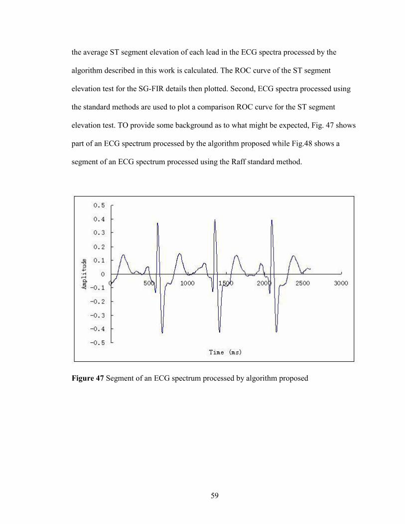
elevation test. TO provide some background as to what might be expected, Fig. 47 shows
part of an ECG spectrum processed by the algorithm proposed while Fig.48 shows a
segment of an ECG spectrum processed using the Raff standard method.
Figure 47 Segment of an ECG spectrum processed by algorithm proposed
60
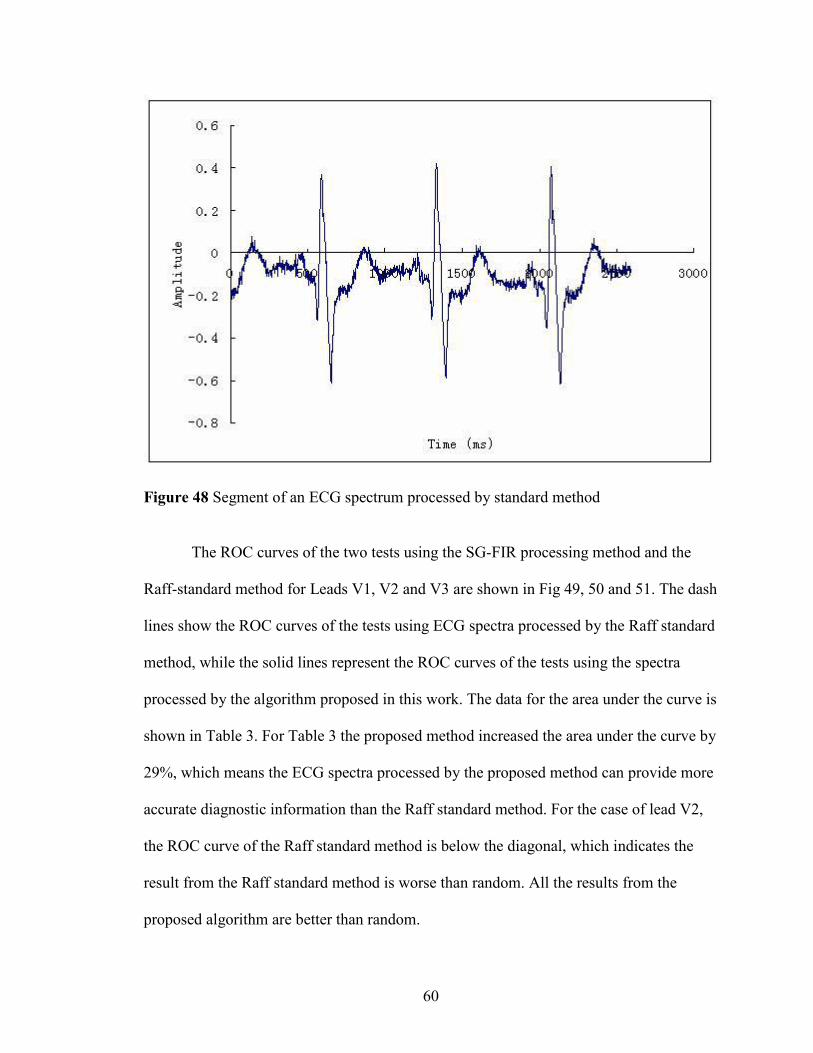
Figure 48 Segment of an ECG spectrum processed by standard method
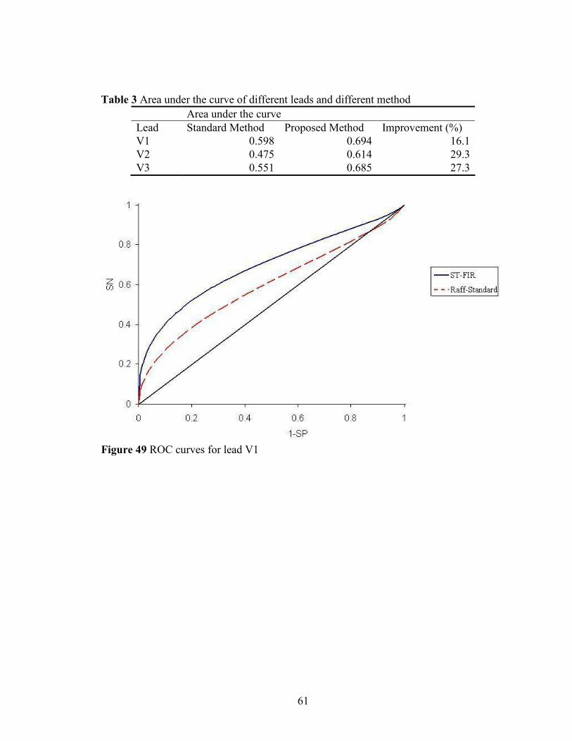
The ROC curves of the two tests using the SG-FIR processing method and the
Raff-standard method for Leads V1, V2 and V3 are shown in Fig 49, 50 and 51. The dash
lines show the ROC curves of the tests using ECG spectra processed by the Raff standard
method, while the solid lines represent the ROC curves of the tests using the spectra
processed by the algorithm proposed in this work. The data for the area under the curve is
shown in Table 3. For Table 3 the proposed method increased the area under the curve by
29%, which means the ECG spectra processed by the proposed method can provide more
accurate diagnostic information than the Raff standard method. For the case of lead V2,
the ROC curve of the Raff standard method is below the diagonal, which indicates the
result from the Raff standard method is worse than random. All the results from the
proposed algorithm are better than random.
61
Table 3 Area under the curve of different leads and different method Area under the curve
Lead Standard Method Proposed Method Improvement (%) V1 0.598 0.694 16.1V2 0.475 0.614 29.3V3 0.551 0.685 27.3
Figure 49 ROC curves for lead V1
62
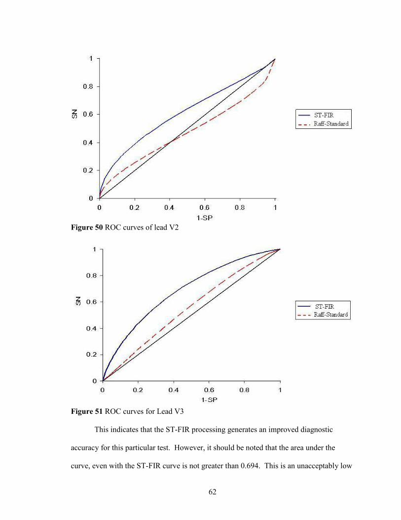
Figure 50 ROC curves of lead V2
Figure 51 ROC curves for Lead V3
This indicates that the ST-FIR processing generates an improved diagnostic
accuracy for this particular test. However, it should be noted that the area under the
curve, even with the ST-FIR curve is not greater than 0.694. This is an unacceptably low
63
value for clinical use. Since only 1 parameter is being used, it is not surprising that the
accuracy is not as high as is needed in clinical practice.
More work clearly needs to be done to determine how many more parameters are
needed before the AUC for the ST-FIR processed signals provides diagnostic accuracy in
the high 90% range. Similarly, it needs to be determined if the accuracy obtained from a
set of several parameters for the ST-FIR procedure is consistently better than the Raff-
standard method. It is known (Raff and Hagan, private communication) that there is no
statistically significant difference when a very large set of parameters is obtained by
either method and the results are then analyzed with a neural network approach. The
reason for this anomalous discrepancy when compared with the results of the current
study shown above and indicated by the fairly noticeable differences in ROC curves
needs to be determined and should be the subject of future research.
64
CHAPTER IV
CONCLUSION
A signal processing algorithm has been developed to reduce high frequency noise
and baseline wander in ECG spectra. The ECG spectra are first processed using a
symmetrical triangle weighting function to reduce the high frequency noise, then by an
FIR high pass filter that is applied to decrease the baseline wander. The results show that
the proposed algorithm is successful in reducing the noise and decreasing baseline
wander. The ROC curves of an ST segment elevation classification tests for myocardial
infarction using clinical ECG spectra processed by the Raff standard method and the
proposed algorithm indicate that the ST-FIR processed data provides improved sensitivity
and specificity for myocardial infarction diagnosis. The area under the ROC curve is
increased by up to 29% for the ST-FIR procedure when compared with the Raff standard
method, which indicates that the proposed signal processing algorithm may provide a
more accurate diagnosis of myocardial infarction.
Further work is required to make the algorithm clinically viable. First, a larger
population is needed for the classification test. Second, the choice of the high and low
pass filter parameters needs more detailed analysis including research to determine
whether improvements may be obtained through use of other related digital filters and
filter design methods. Additional work should also focus on the cutoff frequency,
65
computational efficiency and passband and stopband ripple levels, all assessed by ROC
evaluation and potentially neural network processing of the parameterized results.
66
REFERENCES
1. Gerson, C. M. Cardiac Nuclear Medicine, McGraw Hill, New York, 1987, 309-347.
2. Guiteras, P. Circul. 1982, 65, 1465-1474.
3. Physikalisch-Technische Bundesanstalt, Abbestrasse 2-12, 10587 Berlin, Germany
4. Philips, W. IEEE Trans. Biomed. Eng. 1996, 43, 480–492.
5. Moody, G.B.; Muldrow, W.K.; Mark, R.G. Comput.Cardiol. 1984, 11, 381–384.
6. Ahlstrom, M.L.; Tompkins, W. J. IEEE Trans.Biomed.Eng. 1985, BME-32, 708–713.
7. Bronzino, J. D. Taylor & Francis Group. 2006, 24-4
8. Weaver, J.B.; Yansum, X.; Healy, D.M. Jr.; Cromwell, L.D. Magnet. Resonance Med.
1991, 21, 288–295.
9. Khamene, A.; Negahdaripour, S. IEEE Eng. Med. 2000, Biol. Mag.47, 507–516.
10. Mallat, S.; Zhong, S. IEEE Trans. On Pattern Analysis and Machine Intelligence
1991, 14, 701-732.
11. Donoho, D. L.; Johnstone, I. M. Biometrika 1994, 81, 425-455.
12. Donoho, D. L. IEEE Trans. Inform.Theory 1995, 41, 613-627.
13. Su, L.; Zhao G. Conference proceedings: Annual International Conference of the
IEEE Engineering in Medicine and Biology Society. IEEE Engineering in Medicine and
Biology Society Conference 2005, 6, 5946-9.
14. Gao, W.; Li, H.; Zhuang, Z.; Wang, T. Acta Electronica Sinic. 2003, 32, 238-240.
67
15. Singh, B.N.; Tiwari, A.K. Digital Signal Processing 2006, 16, 275–287
16. Coifman, R. R.; Donoho, D. L. Lecture Notes in Statistics, Springer-Verlag, New
York 1994, 125-150.
17. Bui, T. D.; Chen, G. IEEE Trans. Signal Processing 1998, 46, 3414-3420.
18. Sun, Y.; Chan, K.; Krishnan, S. M. Compuer in biology and medicine 2002, 32, 465-
479.
19. Dai, W.W.; Yang, Z.; Lim, S.L.; Mikhailova, Chee,O. J. Proceedings of the 20th
Annual International Conference of the IEEE Engineering in Medicine and Biology,
Hong Kong 1998, 20, 139 –142.
20. Nikolaev, N.; Zikolov, Z.; Gotechev, A.; Egiazarian, K. Proceedings of 2000 IEEE
International Conference on Acoustics, Speech, and Signal Processing, Istanbul
2000, 6, 3578–3581.
21. Chen, C. S.; Wu, J.L.; Hung, Y.P. IEEE Trans. Signal Process 1999, 47, 1049–1060.
22. Park, K. R.; Lee, C. N. IEEE Trans. Pattern Anal. Mach. Intell.1996, 18, 1121–1126.
23. Maragos, P.; Schafer, R. W. IEEE Trans. Acoust. Speech Signal Process. 1987,
ASSP-35, 1170–1184.
24. Skolnick, M.M.; Butt, D. Proceedings of the 1985 IEEE Workshop on Computer
Architecture Pattern Analysis and Image Database Management, Atlantic, USA,
1985, 438– 443.
25. Sun, Y. Computers in Biology and Medicine 2002, 32, 465–479.
26. Henry Chu, C. H.; Delp, E.J. IEEE Trans. Biomed. Eng. 1989, 36, 262–272.
27. Philips, W. IEEE Transactions on biomedical engineering 1996, 43, 5.
68
28. Lee, J.; Lee, K.; Yoo, S. Conference proceedings : Annual International Conference
of the IEEE Engineering in Medicine and Biology Society. IEEE Engineering in
Medicine and Biology Society. Conference 2004, 1, 224-226.
29. Savitzky, A.; Golay, M. J. E. Anal. Chem. 1964, 36, 1627–1639.
30. Lyons, R. G. Prentice Hall 1996.
31. Rabiner, L. R.; Gold, B. Prentice-Hall, Englewood Cliffs, New Jersey, 1975, 136.
32. McClellan, J. H.; Parks, T. W.; Rabiner, L. R. IEEE Trans. on Audio and
Electroacoustics 1973, AU-21, 515.
33. Shapiro, D. E. Stat Methods Med Res 1999, 8, 113–134.
34. Zweig, M. H.; Campbell, G. Clin. Chem. 1993, 39, 561–577.
35. Obuchowski, N. A. Radiology 2003, 229, 3–8.
36. Metz, C. E. Invest Radiol 1986, 21, 720–33.
37. Lasko, T. A.; Bhagwat, J. G.; Zou, K. H.; Ohno-Machado, L. J. of biomedical
informatics 2005, 38, 404-15.
38. Swets, J. A. Science 1988, 240, 1285–1293.
39. McClish, D. K. Med Decis. Making 1989, 9, 190–195.
40. Zhang, D. D.; Zhou X. H.; Freeman, Jr. D. H.; Freeman J. L. Stat. Med. 2002, 21,
701–1541. Eng J. ROC analysis: web-based calculator for ROC curves. Baltimore:
Johns Hopkins University.
69
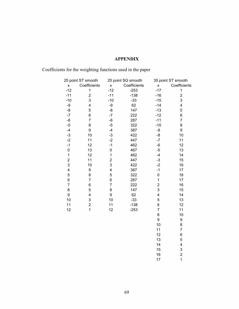
APPENDIX
Coefficients for the weighting functions used in the paper
25 point ST smooth 25 point SG smooth 35 point ST smooth x Coefficients x Coefficients x Coefficients
-12 1 -12 -253 -17 1 -11 2 -11 -138 -16 2 -10 3 -10 -33 -15 3 -9 4 -9 62 -14 4 -8 5 -8 147 -13 5 -7 6 -7 222 -12 6 -6 7 -6 287 -11 7 -5 8 -5 322 -10 8 -4 9 -4 387 -9 9 -3 10 -3 422 -8 10 -2 11 -2 447 -7 11 -1 12 -1 462 -6 12 0 13 0 467 -5 13 1 12 1 462 -4 14 2 11 2 447 -3 15 3 10 3 422 -2 16 4 9 4 387 -1 17 5 8 5 322 0 18 6 7 6 287 1 17 7 6 7 222 2 16 8 5 8 147 3 15 9 4 9 62 4 14 10 3 10 -33 5 13 11 2 11 -138 6 12 12 1 12 -253 7 11 8 10 9 9
10 8 11 7 12 6 13 5 14 4 15 3 16 2 17 1
70
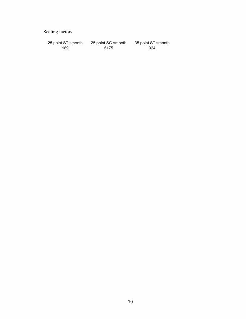
Scaling factors
25 point ST smooth 25 point SG smooth 35 point ST smooth 169 5175 324
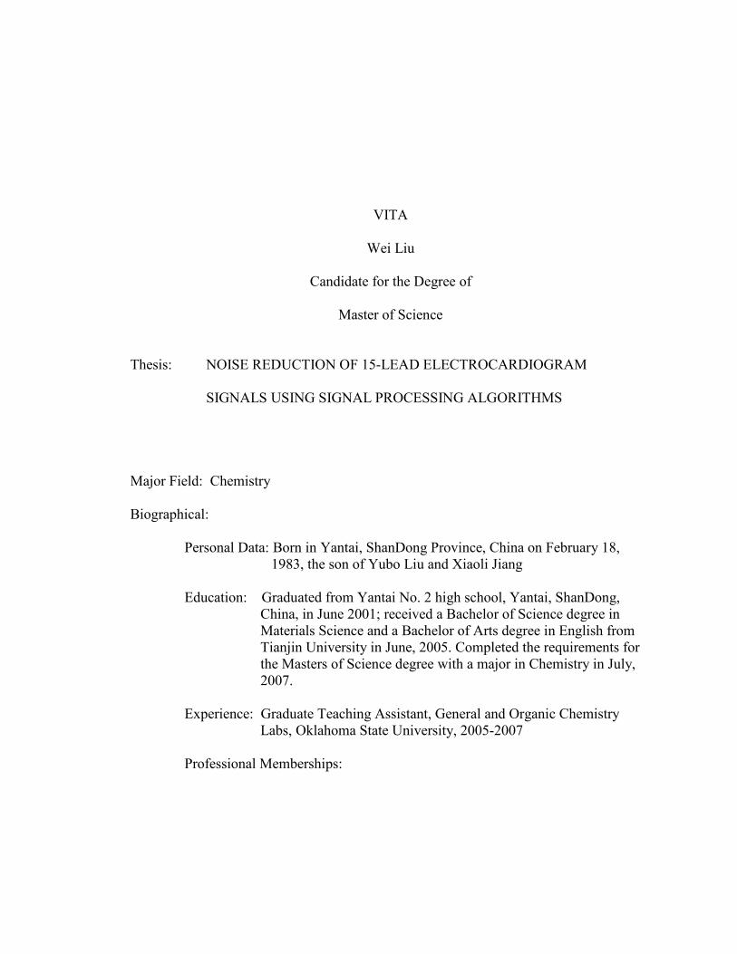
VITA
Wei Liu
Candidate for the Degree of
Master of Science
Thesis: NOISE REDUCTION OF 15-LEAD ELECTROCARDIOGRAM
SIGNALS USING SIGNAL PROCESSING ALGORITHMS
Major Field: Chemistry Biographical:
Personal Data: Born in Yantai, ShanDong Province, China on February 18, 1983, the son of Yubo Liu and Xiaoli Jiang
Education: Graduated from Yantai No. 2 high school, Yantai, ShanDong,
China, in June 2001; received a Bachelor of Science degree in Materials Science and a Bachelor of Arts degree in English from Tianjin University in June, 2005. Completed the requirements for the Masters of Science degree with a major in Chemistry in July, 2007.
Experience: Graduate Teaching Assistant, General and Organic Chemistry
Labs, Oklahoma State University, 2005-2007 Professional Memberships:
Name: Wei Liu Date of Degree: July, 2007 Institution: Oklahoma State University Location: Stillwater, Oklahoma Title of Study: NOISE REDUCTION OF 15-LEAD ELECTROCARDIOGRAM
SIGNALS USING SIGNAL PROCESSING ALGORITHMS Pages in Study: 47 Candidate for the Degree of Master of Science
Major Field: Chemistry Scope and Method of Study: Algorithm development, experiment to test the effect Findings and Conclusions: In the research, a signal processing algorithm is proposed to
reduce the noise and baseline wander in ECG spectra. The ECG spectra are first
processed by symmetrical triangle smooth (can also be considered as a low pass filter) to
reduce the noise, then a FIR high pass filter is applied to decrease the baseline wander.
The ROC curves of the same classification test for myocardial infarction using ECG
spectra processed by the standard and proposed method are plotted. The area under the
curve can be improved up to 29.3%, which indicates the proposed ECG spectra can
provide a more accuracy diagnostic result for myocardial infarction.
ADVISER’S APPROVAL: Mark G. Rockley