Noise-reduction algorithms for optimization- based imaging through

Noise-reduction algorithms for optimization-based imaging through multi-mode fiber

Ruo Yu Gu, Reza Nasiri Mahalati, and Joseph M. Kahn* E. L. Ginzton Laboratory and Department of Electrical Engineering, Stanford University, Stanford, California

94305, USA *[email protected]

Abstract: Three modifications are shown to improve resolution and reduce noise amplification in endoscopic imaging through multi-mode fiber using optimization-based reconstruction (OBR). First, random sampling patterns are replaced by sampling patterns designed to have more nearly equal singular values. Second, the OBR algorithm uses a point-spread function based on the estimated spatial frequency spectrum of the object. Third, the OBR algorithm gives less weight to modes having smaller singular values. In simulations for a step-index fiber supporting 522 spatial modes, the modifications yield a 20% reduction in image error (l2 norm) in the noiseless case, and a further 33% reduction in image error at a 22-dB shot noise-limited SNR as compared to the original method using random sampling patterns and OBR.

©2014 Optical Society of America

OCIS codes: (060.2350) Fiber optics imaging; (100.3010) Image reconstruction techniques; (110.4280) Noise in imaging systems; (170.2150) Endoscopic imaging.

References and links

1. A. Yariv, “Three-dimensional pictorial transmission in optical fibers,” Appl. Phys. Lett. 28(2), 88 (1976). 2. B. Fischer and S. Sternklar, “Image transmission and interferometry with multimode fibers using self-pumped

phase conjugation,” Appl. Phys. Lett. 46(2), 113 (1985). 3. R. N. Mahalati, R. Y. Gu, and J. M. Kahn, “Resolution limits for imaging through multi-mode fiber,” Opt.

Express 21(2), 1656–1668 (2013). 4. I. N. Papadopoulos, S. Farahi, and C. Moser, “High resolution, lenseless endoscope based on digital scanning

through a multimode optical fiber,” Opt. Express 4(2), 17598–17603 (2013). 5. T. Čižmár and K. Dholakia, “Exploiting multimode waveguides for pure fibre-based imaging,” Nat. Commun. 3,

1027 (2012). 6. S. Bianchi and R. Di Leonardo, “A multi-mode fiber probe for holographic micromanipulation and microscopy,”

Lab Chip 12(3), 635–639 (2012). 7. Y. Choi, C. Yoon, M. Kim, T. D. Yang, C. Fang-Yen, R. R. Dasari, K. J. Lee, and W. Choi, “Scanner-free and

wide-field endoscopic imaging by using a single multimode optical fiber,” Phys. Rev. Lett. 109(20), 203901 (2012).

8. S. Farahi, D. Ziegler, I. N. Papadopoulos, D. Psaltis, and C. Moser, “Dynamic bending compensation while focusing through a multimode fiber,” Opt. Express 21(19), 22504–22514 (2013).

9. A. M. Caravaca-Aguirre, E. Niv, D. B. Conkey, and R. Piestun, “Real-time resilient focusing through a bending multimode fiber,” Opt. Express 21(10), 12881–12887 (2013).

10. I. N. Papadopoulos, S. Farahi, C. Moser, and D. Psaltis, “Increasing the imaging capabilities of multimode fibers by exploiting the properties of highly scattering media,” Opt. Lett. 38(15), 2776–2778 (2013).

11. S. Bianchi, V. P. Rajamanickam, L. Ferrara, E. Di Fabrizio, C. Liberale, and R. Di Leonardo, “Focusing and imaging with increased numerical apertures through multimode fibers with micro-fabricated optics,” Opt. Lett. 38(23), 4935–4938 (2013).

12. Y. Choi, C. Yoon, M. Kim, J. Yang, and W. Choi, “Disorder-mediated enhancement of fiber numerical aperture,” Opt. Lett. 38(13), 2253–2255 (2013).

13. B. A. Flusberg, E. D. Cocker, W. Piyawattanametha, J. C. Jung, E. L. M. Cheung, and M. J. Schnitzer, “Fiber-optic fluorescence imaging,” Nat. Methods 2(12), 941–950 (2005).

14. D. L. Donoho, “Compressed sensing,” IEEE Trans. Inf. Theory 52(4), 1289–1306 (2006). 15. E. J. Candes and T. Tao, “Near-optimal signal recovery from random projections: universal encoding strategies?”

IEEE Trans. Inf. Theory 52(12), 5406–5425 (2006). 16. J. A. Buck, Fundamentals of Optical Fibers, 2nd ed. (John Wiley, 2004). 17. J. Mertz, Introduction to Optical Microscopy (Roberts and Company, 2010).

#209564 - $15.00 USD Received 18 Apr 2014; revised 30 May 2014; accepted 1 Jun 2014; published 12 Jun 2014(C) 2014 OSA 16 June 2014 | Vol. 22, No. 12 | DOI:10.1364/OE.22.015118 | OPTICS EXPRESS 15118

18. J. W. Goodman, Introduction to Fourier Optics, 3rd ed. (Roberts and Company, 2004). 19. G. P. Agrawal, Fiber-Optic Communication Systems, 4th ed. (John Wiley, 2010), Chap. 3. 20. A. J. Welch, M. J. C. Van Gemert, W. M. Star, and T. Optics, Optical-Thermal Response of Laser-Irradiated

Tissue, 2nd ed. (Springer, 2011), Chap. 3. 21. A. J. Welch, “The thermal response of laser irradiated tissue,” IEEE J. Quantum Electron. 20(12), 1471–1481

(1984). 22. A. L. McKenzie, “Physics of thermal processes in laser-tissue interaction,” Phys. Med. Biol. 35(9), 1175–1210

(1990). 23. S. W. Allison, G. T. Gillies, D. W. Magnuson, and T. S. Pagano, “Pulsed laser damage to optical fibers,” Appl.

Opt. 24(19), 3140–3144 (1985). 24. M. B. Shemirani, W. Mao, R. A. Panicker, and J. M. Kahn, “Principal modes in graded-index multimode fiber in

presence of spatial- and polarization-mode coupling,” J. Lightwave Technol. 27(10), 1248–1261 (2009).

1. Introduction

The use of multi-mode fibers (MMFs) for imaging has long been of interest [1,2], and the past few years have seen particularly productive developments in the field of MMF endoscopic imaging [3–12]. An endoscope employing one MMF provides resolution superior to, and is much more compact than, current commercial fiber endoscopes, which may use either a bundle of single-mode fibers or one single-mode fiber with a scanning probe head [13]. Light signals propagating through a MMF are subject to random scattering by index imperfections, bends and other perturbations. All endoscopic MMF imaging methods, prior to image recording, employ some calibration method that requires access to both ends of the fiber. Since bending changes a fiber’s propagation characteristics, all MMF endoscopes to date have been rigid, although compensation of bending has been investigated [8,9].

One endoscopic MMF imaging method [3] uses random intensity patterns to sample an object and employs an optimization-based image reconstruction (OBR) algorithm. This method at once enhances the resolution to four times the number of spatial modes propagating in the MMF and requires the least complicated calibration setup among all imaging methods. The OBR algorithm decomposes the set of random intensity sampling patterns into a set of intensity modes using a singular-value decomposition (SVD), and reconstructs the image as a linear combination of the intensity modes based on the powers reflected from the object when sampled by the random intensity patterns. This technique is similar to compressed sensing [14,15].

Despite the advantages of this imaging method, reconstructed images were found to be noisy [3], suggesting that noise amplification occurs in OBR. In this paper, we quantify the noise amplification occurring in OBR, and describe three methods to reduce it. First, we sample the object using a set of intensity patterns designed to have singular values more equalized than a set of random intensity patterns. Second, we modify the OBR algorithm to use a point-spread function (PSF) based on the estimated spatial frequency spectrum of the object. Third, we diminish the influence of intensity modes with smaller singular values on the reconstructed image. Using simulation, we compare images obtained using noise-reduced OBR to those obtained by localized spot sampling with localized reconstruction in the presence of noise, and subject to constraints on the number of sampling patterns and the power illuminating the object through the MMF.

The remainder of this paper is as follows. In Section 2, we describe the imaging system and a model for the electric fields illuminating the object and captured by the MMF, and briefly review the OBR algorithm described in [3]. In Section 3, we analyze the image noises obtained using OBR or localized sampling/reconstruction and quantify the noise amplification of OBR. In Section 4, we introduce three methods to improve the noise performance of OBR. In Section 5, we present simulated images obtained using OBR or localized sampling/reconstruction under the constraints mentioned above. We discuss the results in Section 6 and provide conclusions in Section 7.


2. Model for object sampling and image reconstruction

2.1 Imaging system and model for electric fields

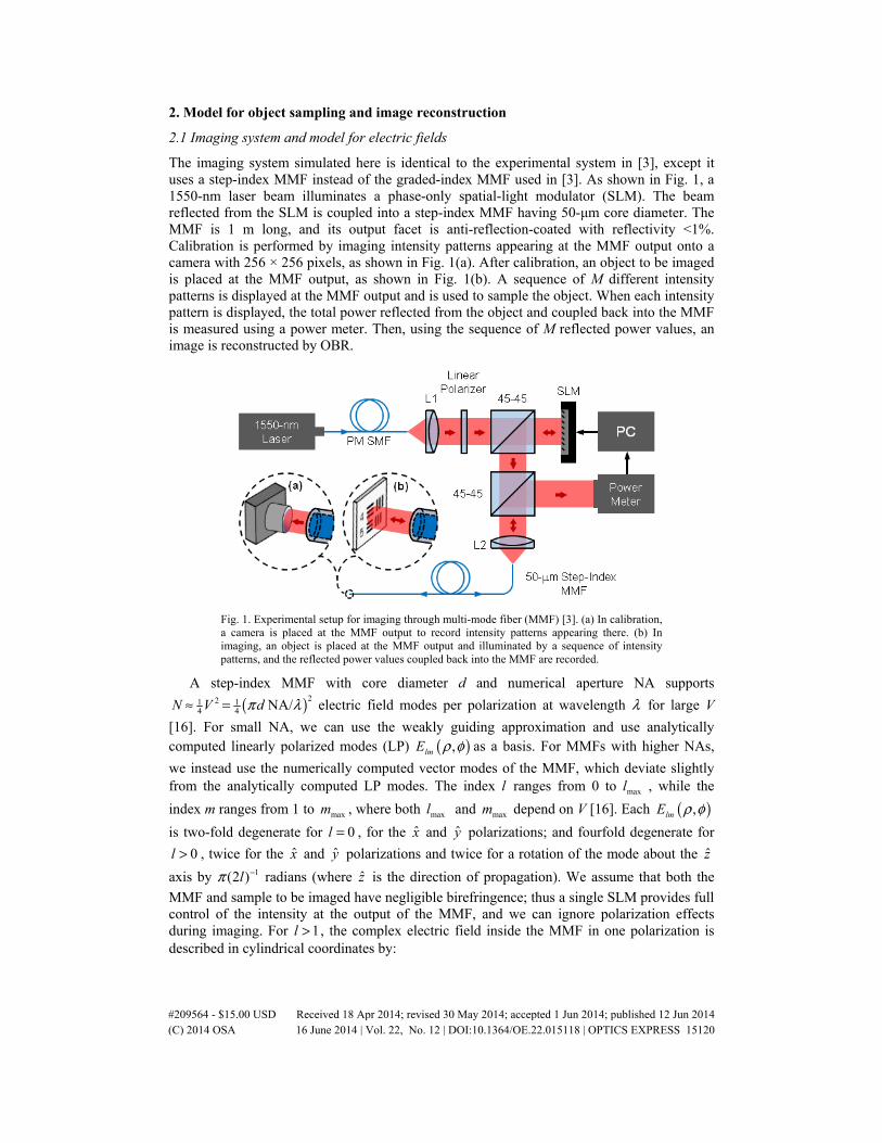
The imaging system simulated here is identical to the experimental system in [3], except it uses a step-index MMF instead of the graded-index MMF used in [3]. As shown in Fig. 1, a 1550-nm laser beam illuminates a phase-only spatial-light modulator (SLM). The beam reflected from the SLM is coupled into a step-index MMF having 50-μm core diameter. The MMF is 1 m long, and its output facet is anti-reflection-coated with reflectivity <1%. Calibration is performed by imaging intensity patterns appearing at the MMF output onto a camera with 256 × 256 pixels, as shown in Fig. 1(a). After calibration, an object to be imaged is placed at the MMF output, as shown in Fig. 1(b). A sequence of M different intensity patterns is displayed at the MMF output and is used to sample the object. When each intensity pattern is displayed, the total power reflected from the object and coupled back into the MMF is measured using a power meter. Then, using the sequence of M reflected power values, an image is reconstructed by OBR.

Fig. 1. Experimental setup for imaging through multi-mode fiber (MMF) [3]. (a) In calibration, a camera is placed at the MMF output to record intensity patterns appearing there. (b) In imaging, an object is placed at the MMF output and illuminated by a sequence of intensity patterns, and the reflected power values coupled back into the MMF are recorded.

A step-index MMF with core diameter d and numerical aperture NA supports

( )1 14 4

22 NA/N V dπ λ≈ = electric field modes per polarization at wavelength λ for large V

[16]. For small NA, we can use the weakly guiding approximation and use analytically computed linearly polarized modes (LP) ( ),lmE ρ φ as a basis. For MMFs with higher NAs,

we instead use the numerically computed vector modes of the MMF, which deviate slightly from the analytically computed LP modes. The index l ranges from 0 to max l , while the

index m ranges from 1 to maxm , where both maxl and maxm depend on V [16]. Each ( ),lmE ρ φ

is two-fold degenerate for 0l = , for the x and y polarizations; and fourfold degenerate for

0l > , twice for the x and y polarizations and twice for a rotation of the mode about the z

axis by 1(2 )lπ − radians (where z is the direction of propagation). We assume that both the

MMF and sample to be imaged have negligible birefringence; thus a single SLM provides full control of the intensity at the output of the MMF, and we can ignore polarization effects during imaging. For 1l > , the complex electric field inside the MMF in one polarization is described in cylindrical coordinates by:


1

,2

1 ,( , ) ( )sin( ) (core)

( , ) ( )sin( ) (cladding)

lm l m

lm l ml

E c J l

E c K l

φ κ φ

φ γ φ

ρ ρ

ρ ρ

=

= (1)

where ρ and φ denote radius and azimuthal angle; ( )Jν ρ is the Bessel function of the first

kind of order ν ; ( )Kν ρ is the modified Bessel function of the second kind of order ν ; ,l mκ

and ,l mγ are constants that depend on NA , d and λ ; and 1c and 2c are real normalization

constants. The expressions for the electric field for 1l ≤ are similar. Let P1 denote the MMF output plane and P2 denote the object plane. At P1, the total

forward-propagating electric field is a linear combination of the LP modes, and is described by:

( ) ( )max max max, ,

10, 0, 0

, , ,ql m

P f lmq lmql m q

E x y c E x y= = =

= (2)

where lmqc is a complex amplitude. A change of basis from cylindrical ( ),ρ φ to Cartesian

( ),x y co-ordinates has been made from Eq. (1), and the index q has been added to

differentiate between the degeneracies of ( ),lmE x y .

Free-space propagation over a distance z is represented by [ ]zP , and is modeled here by

Rayleigh-Sommerfeld diffraction [17]. At P2 the total forward-propagating electric field is thus:

( ) ( )max max max,,

20, 0, 0

, , ,l m

P f lmq lmql m

q

qzE x y Pc E x y

= = =

= (3)

At P2, a back-propagating electric field is generated by reflection from the object. We assume that the electric field reflects from a thin surface and reflection can be described by scalar diffraction theory [18], meaning that the reflected electric field is the product of the incident electric field and the complex reflectance of the object in each polarization on plane P2:

( ) ( ) ( )2 2, , , .P b P fE x y r x y E x y= (4)

The power coupled back into the MMF is given by:

( ) ( )max max max, 2,

20, 0, 0

, , .l m

lmq z P bl

q

m q

p E x y P E x y dxdy∞ ∞

−= = = −∞−∞

= (5)

The power is assumed to be conserved in propagation through the MMF, and is measured by a power meter.

2.2 Optimization-based reconstruction algorithm

The relation between p and ( ),r x y in Eqs. (4) and (5) is not linear. Solving for ( ),r x y from

p using Eq. (5) requires coherent detection of ( )2 ,P fE x y and is in general computationally

difficult for a MMF with the number of modes required for imaging. However, if we instead assume that the fraction of the reflected light recaptured by the MMF is independent of the object, and that the object ( ),r x y has equal reflectivity in both polarizations, Eq. (5) can be

replaced by:


( ) ( )2

2, ,P fp c E x y r x y dxdy

∞ ∞

−∞−∞

= (6)

( ) ( )2 2

2 , ,P fp cE x y r x y dxdy∞ ∞

−∞−∞

= (7)

( ) ( )2 , , ,P fp I x y R x y dxdy∞ ∞

−∞−∞

= (8)

where c accounts for the fraction of the reflected light recaptured by the MMF for the

sampling pattern ( )2 ,P fE x y and any object ( ),r x y ; c can be computed using Eqs. (4) and

(5) and assuming ( ),r x y is a perfect mirror, or measured experimentally. In Eq. (8),

( )2 ,P fI x y is the intensity pattern at P2 measured by the camera during calibration and then

multiplied by 2

c . We note that in actuality c is not independent of ( ),r x y , so the

approximation used in Eq. (6) effectively introduces an error in p. The impact of this error will be seen in subsequent images, but the effect is small if the ( )2 ,P fE x y used to sample the

object are statistically similar (e.g. random patterns). If we employ a sequence of M intensity patterns ( )2 ,P fI x y during imaging, we obtain a

corresponding 1M × vector of powers p. If we discretize ( )2 ,P fI x y and ( ),R x y to a grid

of L points and reshape them into row vectors, we obtain the simple expression:

,p = Ir (9)

where p is an 1M × vector of all p , I is an M L× matrix in which each row represents an

intensity sampling pattern, and r is an 1L × vector representing the intensity reflectance of the object. This equation is linear, and the image w can then be reconstructed using [3]:

1 ,− Tw = VD U p (10)

where TI = UDV is the compact singular value decomposition of I , and:

,1,

1 / for 4.

0 otherwisei j

i j

D i j ND− = ≤

=

(11)

3. Noise of image reconstruction methods

In the previous section we assumed that the received power specified in Eq. (9) is noiseless. We now introduce noise. Given an apparatus, as the optical power is increased, the limiting noise source progresses from thermal to shot to intensity noise [19]. In the following section, we analyze all three regimes.

3.1 Noise of optimization-based image reconstruction

We assume that the calibration images I are noiseless. This assumption is valid if sufficient time is available for calibration using the camera to make noise negligible and there is no movement of the MMF during imaging. The noisy reconstructed image is then:

( )1− Tw = VD U p + n (12)

1−T T Tw = VV r + V D U n (13)


1 ,−≡ T Tw V D U n (14)

where we have defined w as the image error due to noise. Here, n is a vector of random noises, and depends on whether thermal, shot or intensity noise dominates. In the three cases, it is given by:

thermal ˆ (thermal)σn = n (15)

shot ˆ (shot)σn = n p (16)

intensity ˆ (intensity),σn = n p (17)

where is the Hadamard (elementwise) product and n is a vector of i.i.d. Gaussian random variables with mean 0 and variance 1. The amount of noise amplification occurring in OBR

can be quantified from the relation between the l2 norm of w , given by 2

1

L

iiE w

= , and n.

For intensity noise, the relevant equations are:

= Tp UDV r (18)

intensity ˆσn = n p (19)

1− Tw = VD U n (20)

,≡ Tn U n (21)

In Eq. (21), n is the component of the noise in the basis of intensity modes, which is useful in the following derivation. We model r as a vector of i.i.d. uniformly distributed random

variables between 0 and 1. Solving for 2

1

L

iiE w

= , we have:

( )422 1 2 2 2 2

1 1 1 1 1

4 4 1L N

i ii i ii i i iii i i i

N N M

i

E w E D n D E n E n DM

− − −

= = = = =

= = ≈

(22)

( ) ( )22 2 2 2 2 2intensity intensity

1 1 1 1

.M M M M

i i i i ii i i i

E n E n E n p pσ μ σ σ= = = =

= = = + (23)

Throughout Eqs. (22) and (23), we have used the fact that unitary matrices preserve the l2 norm. The approximation in Eq. (22) is accurate as long as all patterns in I have total powers within the same order of magnitude. Similarly, we find:

( ) [ ]11 1

1

2

L L

i i ij ijj j

p E E r I Iμ= =

= = = Ti r (24)

( ) ( )2 2 2 21

1 1

4 41 1

12,i ii ii

i i

N N

p r D DM M

σ σ= =

= = (25)

where iTi is the ith row of I . We note that ( ) ( )22 2 2

intensity intensity1 1

M M

i ii ip pσ μ σ σ

= = , and so

discard that term in Eq. (23). Using Eqs. (22)–(25), we finally have:

2

2 2 2intensity

1 1

4

1 1

1 1.

2

L M L

i ii iji i i j

N

E w D IM

σ−

= = = =

= (26)

Equivalently, after dividing by the number of image pixels and taking the square root, the root mean square deviation (RMSD) of the image error is given by:


( )2

2intensity

1 1 1

41 1 1(intensity noise)

2

M L

i ii iji i

N

j

w D IL M

σ σ−

= = =

=

(27)

( ) 2

1 1

4

sh t1

o

1 1 1(shot noise)

2

M L

i ii iji i

N

j

w D IL M

σ σ−

= = =

=

(28)

( )4

thermal2

1

1(thermal noise),i ii

i

N

w DL

σ σ−

=

= (29)

where the expressions for shot and thermal noise are found in a similar manner. We see that

for all three types of noise, ( )iwσ is proportional to 4 2

1

1 N

iiiD

L−

= , but with different

multiplicative factors.

3.2 Noise of localized reconstruction

In this imaging method, the sampling patterns at the MMF output plane P2 are localized spots on a regular grid of points. As each sampling pattern illuminates the object, the power reflected from the object yields the intensity in the corresponding region of the reconstructed image, a process termed localized reconstruction [3]. For localized reconstruction using M spots, the corresponding relation between the noise n, spot sampling patterns I and image w is:

( ) w = T s Ir + n (30)

( ) ,w = T s n (31)

where T is a L M× matrix that implements sinc interpolation to upsample the image, each row of I represents samples of the smallest spot that can be formed at the corresponding grid point using the propagating modes of the MMF [3], and s is a 1M × vector of the reciprocal of the power that couples back into the MMF when imaging a perfect mirror using I . The noises n are as given in Eqs. (15)–(17). The corresponding RMSDs of image error due to noise are: ( ) intensity

12 (intensity noise)iwσ σ= (32)

( )1

shot1 1

1(shot noise)

2

M P

i iji j

w IM

σ σ−

= =

=

(33)

( )2

thermal1 1

1(thermal noise),

M P

i iji j

w IM

σ σ−

= =

=

(34)

where we have used the fact that sinc interpolation leaves ( )iwσ unchanged. With these

equations, we may define noise amplification as the ratio of the image error RMSDs for OBR, given by Eqs. (27)–(29), to the image error RMSDs using localized reconstruction, given by Eqs. (32)–(34).

4. Techniques to improve noise performance

4.1 Sampling using optimal patterns

The dependence of the image error ( )iwσ on the singular values of I in Eqs. (27)–(29)

suggests that noise amplification can be reduced by choosing a specific set of sampling patterns I with more equalized singular values. We heuristically expect a grid of spots


(identical to that used in localized sampling and reconstruction) to be a good set of sampling patterns: among all possible sampling patterns satisfying the physical constraint of positive intensity ( 0 ,ijI i j≥ ∀ ), the overlap integral between different sampling patterns is minimized

for a grid of spots, which is a good characteristic for minimizing4 2

1

N

iiiD−

= . We briefly note

that forming specific sampling patterns is necessarily more difficult than forming random patterns, since light undergoes random mode coupling during MMF propagation. Conveniently, methods have been described to form the entire set of spot patterns with total time linearly proportional to the number of modes N [4–6].

The impacts of shot and thermal noise are inversely dependent on the integrated total power in the sampling patterns, so it is desirable to maximize the total power in these patterns. However, this power must be limited to prevent damage to tissue [20–22], which occurs at powers well below those that cause any damage to the MMF [23]. Tissue damage is typically caused by thermal effects, which depend on the irradiance incident on the tissue [22], so we constrain the maximum irradiance of each sampling pattern such that max ,ijI I i j< ∀ (here we

use the terms irradiance and intensity interchangeably in referring to the power per unit area). This constraint is particularly important when MMFs with high NA are used, as they permit the total power to be concentrated in a high-irradiance spot that is much smaller than the MMF core. However, since thermal effects are not directly localized to the irradiated area, a large and uniform sampling pattern can cause more damage than a smaller one with the same irradiance. To account for this, we additionally constrain the total power of each sampling

pattern such that max1

L

ijjI P i

=< ∀ .

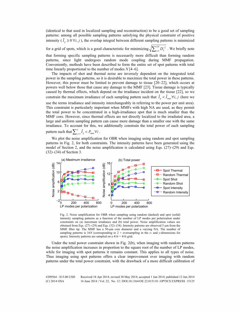
We plot the noise amplification for OBR when imaging using random and spot sampling patterns in Fig. 2, for both constraints. The intensity patterns have been generated using the model of Section 2, and the noise amplification is calculated using Eqs. (27)–(29) and Eqs. (32)–(34) of Section 3.

Spot ThermalRandom ThermalSpot ShotRandom ShotSpot IntensityRandom Intensity

0 200 400 600−2

2

6

10

14

LP modes per polarization

Noi

se a

mpl

ifica

tion

(dB

)

(a) Maximum irradiance

0 200 400 600

4

8

12

16


Noi

se a

mpl

ifica

tion

(dB

)

0 200 400 600

4

8

12

16


Noi

se a

mpl

ifica

tion

(dB

)

(b) Total power

Fig. 2. Noise amplification for OBR when sampling using random (dashed) and spot (solid) intensity sampling patterns as a function of the number of LP modes per polarization under constraints on (a) maximum irradiance and (b) total power. Noise amplification values are obtained from Eqs. (27)–(29) and Eqs. (32)–(34). Intensity patterns are observed 5 μm from the MMF fiber tip. The MMF has a 50-μm core diameter and a varying NA. The number of sampling patterns is 16N (corresponding to 2 × oversampling in the x- and y-dimensions for spots). Intensity patterns are sampled on a 416 × 416 grid.

Under the total power constraint shown in Fig. 2(b), when imaging with random patterns the noise amplification increases in proportion to the square root of the number of LP modes, while for imaging with spot patterns it remains constant. This applies to all types of noise. Thus imaging using spot patterns offers a clear improvement over imaging with random patterns under the total power constraint, with the drawback of a more difficult calibration of


the imaging apparatus. Conversely when operating under the maximum irradiance constraint of Fig. 2(a), spot patterns have less noise amplification than random patterns only for intensity noise. Thus imaging using random patterns is superior unless intensity noise dominates.

The results of Fig. 2 are for a specific MMF core diameter of 50 μm, but we expect the results to be similar for a constant number of modes independent of core diameter (with the distance to the object scaled according to the Rayleigh range of the MMF [3]). We note also that MMFs are commonly available with well over 500 modes, but it may not be possible to use all these modes for imaging due to time constraints; for example, for 500 modes and a grid of spots with an oversampling factor of 2 × in the x- and y-dimensions, 8000 spots need to be sequentially formed during imaging to exploit all the modes.

4.2 Exploiting known properties of the object

In [3], the image reconstruction algorithm was chosen under the assumption that nothing is known about r, the object to be imaged. However, at a minimum we do know that r must be positive and have a limited spatial frequency bandwidth. If instead r were i.i.d., it would have a uniform spatial frequency spectrum up to the spatial sampling rate of the camera used to record the intensity patterns. For realistic objects, the spatial frequency spectrum drops off well before this. With this motivation, we modify the OBR algorithm to exploit any information known about the spatial frequencies of the object. This requires a more general objective function than the one described in [3], which was:

22arg min s.t. ,− =T

wp Iw V w 0 (35)

where p , I and w are defined in Section 2, V is the matrix of right singular vectors defined

in Section 2, and 2V is a submatrix of V such that 1 2[ ]=V V V , with 1V containing the

right singular vectors that have singular values deemed to be significant (chosen here as >1% of the maximum singular value).

Instead of Eq. (35), we minimize the l2 norm between the object intensity reflectance and the image:

2

arg min −w

w r (36)

Note that we do not know r. For consistency, we show below that Eq. (35) is equivalent to Eq. (36) with the constraint that =p wI when r is i.i.d. with mean 0. For Eq. (35):

( )

( )

2 2 22

22

1 22

arg min s.t. arg min s.t.

arg min s.t.

arg min s.t.

− = = − =

= − =

= − =

T T T T

T

w

T

T T

w

w

w

p I V w 0 UDV r UDV w V w 0

DV r w V w 0

w r V

w

V w 0

(37)

In the above, the final equality is valid because the minimum of the norm is 0. We have made the approximation that small singular values are zero. For Eq. (36):

( )

( ) ( )( )( )

1 12 2

1 2

22

2 2

1

arg min ars g min

arg min

arg min s

.t. s.t.

.t.

=

=

− = = − =

− + −

− =

w w

w

w

T T T

T T

T T

w r p I V w r V r V w

V w r V w r

V w r V w 0

w

(38)


In the above, the final line is valid because r is i.i.d. and equally likely to be negative or positive, so 2 =TV w 0 minimizes the l2 norm. Equation (38) has the same result as Eq. (37)

above. We note that the continuous form of Eq. (36) allows a simplification if we assume that the

point-spread function ( ),q x y of the image is spatially invariant. In that case:

( ) ( )Image

2, ,w x y r x y dxdy− ∬ (39)

( ) ( ) ( )( ) 2

Image

, , ,r x y q x y x y dxdyδ ∗ − ∬ (40)

( ) ( ) ( )( )Image

2

, , , ,r x y q x y x y dxdyδ − ∬ (41)

where r , q and δ are the Fourier transforms of the original functions and ∗ denotes

convolution. In minimizing Eq. (36), we restrict ourselves to solutions of the form:

1 ,−= TpDw V U (42)

where TU and 1−D are the same as in Eq. (10), and V remains to be determined. We chose

Eq. (42) since it can be simplified to 1 = Tw VV r , which allows us to interpret iT Tv V as the

point-spread function of the image at pixel i, where iTv is the ith row of V . We know the

objective function for the optimal PSF from Eq. (41), and so we use the following equation to solve for every i

Tv :

( ) ( )DFT 1 D2

FT DFTarg min ,i

i i= −T

T T T T

v

v r F v V F δ F

(43)

where DFTF is the 2D DFT matrix, and δ is a vector of the discrete delta function centered at

the pixel corresponding to iTv . Equations (42) and (43) are all the equations required to

reconstruct the image, and replace Eq. (5). Using the electric field model described in Section 2, we simulate imaging of an object in

MATLAB. We compare the images obtained with the original and new algorithms in Fig. 3.


−30

−15

0

15

30

y(μ

m)

(a) 9.3%

30

−30 −15 0 15 30−30

−15

0

15

x (μm)

y(μ

m)

(c)

−30 −15 0 15 30x (μm)

(d)

(b) 7.5%

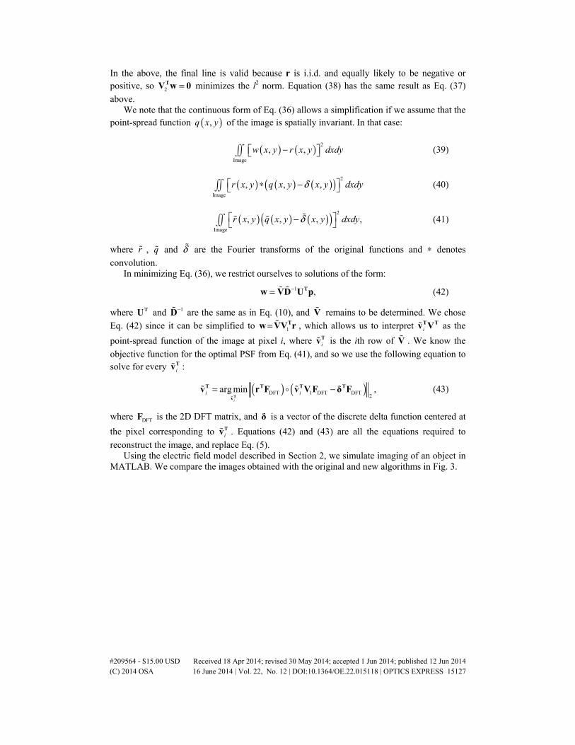
Fig. 3. Images reconstructed using OBR: (a) original algorithm and (b) new algorithm using an estimate of the object spatial frequency spectrum. Also shown are: (c) the object reflectance and (d) the object providing the estimated spatial frequency spectrum, which is unrelated to the

actual object. In (a) and (b), values of the image error RMSD ( )iwσ within the MMF core

are given as a percent of the maximum image intensity. Intensity patterns and object are at 5 μm from the MMF fiber tip. The MMF has 50-μm core diameter and 0.45 NA. The number of sampling patterns is 16N (corresponding to 2 × oversampling in the x- and y-dimensions for spots). Intensity patterns are sampled on a 256 × 256 grid.

We see that the image quality is substantially improved when using the new algorithm, which reduces the image error RMSD from 9.3% to 7.5% of the maximum image brightness – or equivalently, an increase in the peak signal-to-noise ratio from 20.6 to 22.5 dB. We do note that to use Eq. (43), it is necessary to know r. This seems to present a paradox: if we know r, we already have a perfect image of the object and imaging is unnecessary. In practice, however, the improvement shown in Fig. 3 can be obtained even if we have only an estimate of the spatial frequency spectrum of r. The r used in Eq. (43) is shown in Fig. 3(d), and differs substantially from the actual r shown in Fig. 3(c).

We also briefly mention the issue of computation time. Equation (43) is a quadratic optimization problem with N variables, which can be solved efficiently by convex optimization methods. In practice, the amount of time to solve Eq. (43) on a personal computer is under 1 s. However, the number of separate i

Tv that must be solved is equal to L,

the number of pixels in the final image (e.g., L = 2562 for a 256 × 256 pixel image). Hence, real-time computation of Eq. (43) for V requires solving for the different i

Tv in parallel. We

finally note that V is not unitary, and thus the noise amplification no longer depends on the

singular values of TUDV but instead on the singular values of the matrix TUDV , which are not the diagonal elements of D. In practice, the changes to the noise amplification are minor.

4.3 Noise-reduced image reconstruction

Noise amplification can be further mitigated during image reconstruction by adding a constraint to the elements of each i

Tv :


,i iα< ∀T Tv d (44)

where d is a row vector of the diagonal elements of D and α is a real constant to be determined. Together with Eq. (43), this becomes:

( ) ( )DFT 1 DFT2

DFTarg min s.t. .i

i i i α= − <T

T T T T T T

v

v r F v V F δ F v d

(45)

From Section 3, the noise amplification depends on the singular values of TUDV . When Eq. (51) is used instead of Eq. (43), the singular values are more equalized and thus the contribution to noise from low singular values is limited. However, by limiting the contribution to the image by intensity modes with low singular values, the resulting image has reduced resolution. The choice of α determines the tradeoff between noise amplification and resolution; when α is sufficiently high, Eq. (45) reduces to Eq. (43). We denote this value of α as maxα , given by 1

max max( )α −= VD , where V is the solution to Eq. (43).

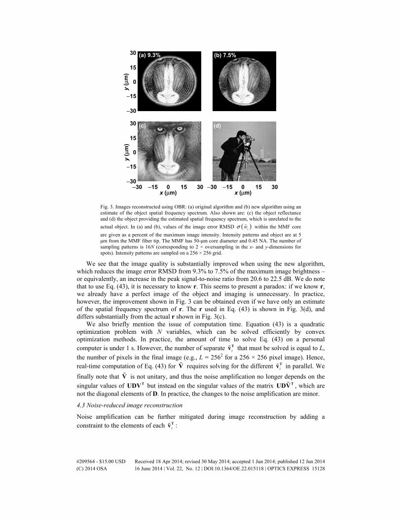
Using the electric field model described in Section 2, we simulate imaging of an object in MATLAB. We compare the images obtained using Eqs. (42) and (43) and Eqs. (44) and (45) in Fig. 4.

−30 −15 0 15 30−30

−15

0

15

30

x (μm)

y(μ

m)

(a) 14.0%

−30 −15 0 15 30x (μm)

(b) 9.4%

Fig. 4. Images reconstructed using OBR: (a) using original method of Eqs. (42) and (43), and (b) using reduced-noise method of Eqs. (44) and (45). The ratio of the noise constraint to the

maximum noise constraint is max/ 10 dBα α = − . The shot noise-limited SNR is

noise / 22 dBσ = −p , where p is the average power. Values of the image error RMSD

( )iwσ within the MMF core are given as a percent of the maximum image intensity. The

intensity patterns and object are at 5 μm from MMF fiber tip. The MMF has 50-μm core diameter and 0.45 NA. The number of sampling patterns is 16N (corresponding to 2 × oversampling in the x- and y-dimensions for spots). The intensity patterns are sampled on a 256 × 256 grid.

We observe that the image reconstructed using Eqs. (44) and (45) is less noisy, with a reduction in image error RMSD from 14.0% to 9.4%. For every noise SNR there is an optimal value of α that balances the image errors due to reduced resolution and noise, and thus minimizes the total image error. When r is unknown, the optimal value of α is also unknown, but α can be chosen such that the image error RMSD is subjectively minimized, which is how α has been chosen here. Using Eqs. (44) and (45) reduces thermal, shot and intensity noise equally, and also reduces the error introduced due to the approximation of Eq. (6). Since this is always present even in the noiseless case, conservative (large) values of α lead to reductions in image error RMSD even when there is no noise.


5. Comparison of image quality

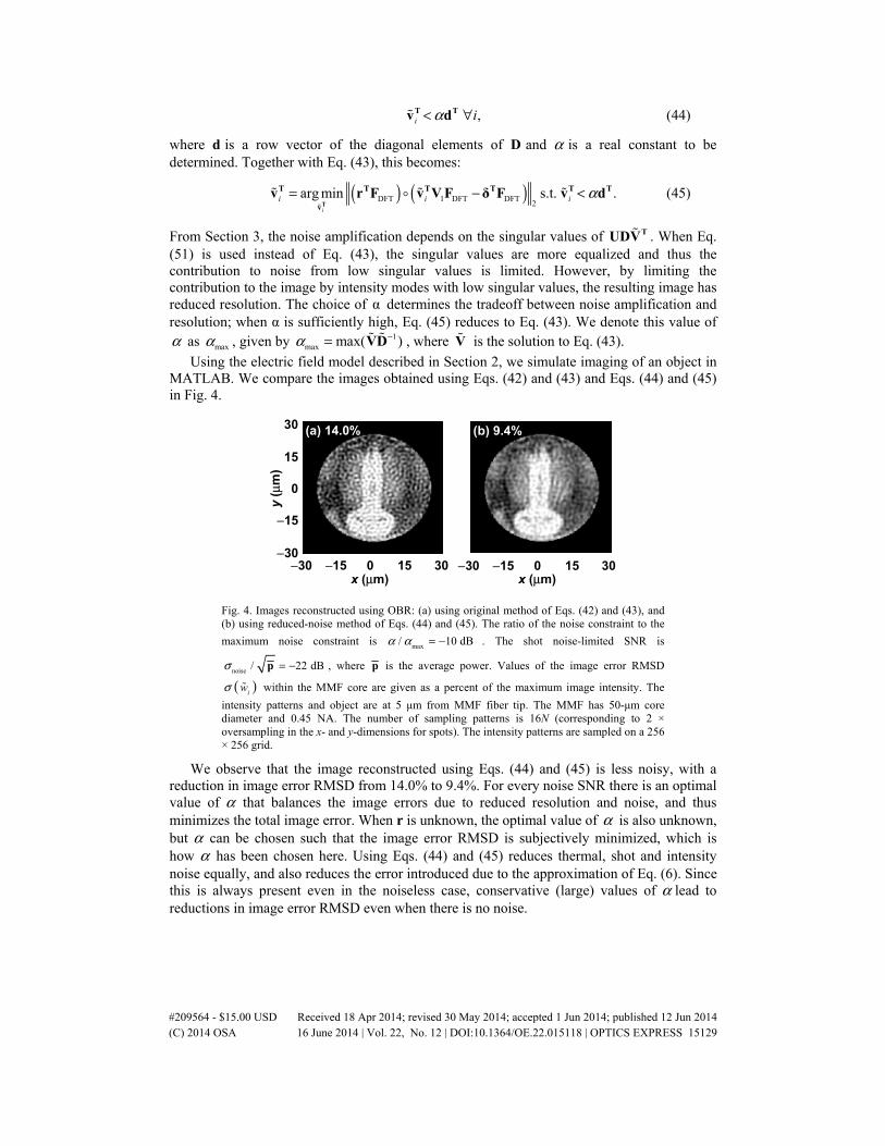
To directly compare the image error between images reconstructed using OBR and localized reconstruction, we simulate imaging an object using both methods in the presence of noise and plot the image error versus the power noise in Fig. 5. The apparatus and noise model are as described in Sections 2-3. The imaged object is shown previously in Fig. 3(d). In the plots

of Fig. 5, we have normalized the noise values: at any SNR, intensity shot thermal/ /p pσ σ σ= = ,

where p denotes the average measured power for imaging using OBR. Equal values of

thermalσ , shotσ , intensityσ and equal numbers of sampling patterns were used for both OBR and

localized reconstruction. Results for both the maximum irradiance and total power constraints are shown in Fig. 5. For the maximum irradiance constraint the sampling patterns for OBR are random, while for the total power constraint the sampling patterns for OBR are spots, for reasons described in Section 4.1.

Localized Thermal

OBR Thermal

Localized ShotOBR Shot

Localized Intensity

OBR Intensity

10 15 20 250.09

0.14

0.19

0.24

Power SNR (dB)

Ima

ge

err

or

per

pixe

l

(b) Total power

10 15 20 250.08

0.16

0.24

0.32

Power SNR (dB)

Ima

ge

err

or p

er p

ixel

(a) Maximum irradiance

Fig. 5. Errors of images reconstructed using OBR (dashed lines) and localized reconstruction (solid lines) as a function of power noise levels under constraints on (a) maximum irradiance and (b) total power. The intensity patterns and object are at 5 μm from MMF fiber tip. The MMF has 50-μm core diameter and 0.45 NA. The number of sampling patterns is 16N (corresponding to 2 × oversampling in the x- and y-dimensions for spots). Intensity patterns are sampled on a 256 × 256 grid.

The noise amplification curves shown in Fig. 5 behave as predicted based on Fig. 2. For low levels of noise, images reconstructed using OBR have a lower image error RMSD than those using localized reconstruction, because the former have higher resolution. For high levels of noise, images reconstructed using OBR have higher image error RMSD than localized reconstruction, due to noise amplification. Under the maximum irradiance constraint, the image error using OBR is less than that of localized reconstruction for all thermal noise levels, and for noises up to −18 dB and −19 dB for shot and intensity noises, respectively. When imaging using spot patterns under the total power constraint, the image error using OBR is less than that of localized reconstruction for noises up to −15 dB, −15 dB and −16 dB for thermal, shot and intensity noises, respectively.


−30

−15

0

15

30

y(μ

m)

(a) 9.8% (b) 11.8% (c) 20.3%

−30 −15 0 15 30−30

−15

0

15

30

x (μm)

y(μ

m)

(d) 12.2%

−30 −15 0 15 30x (μm)

(e) 12.4%

−30 −15 0 15 30x (μm)

(f) 13.1%

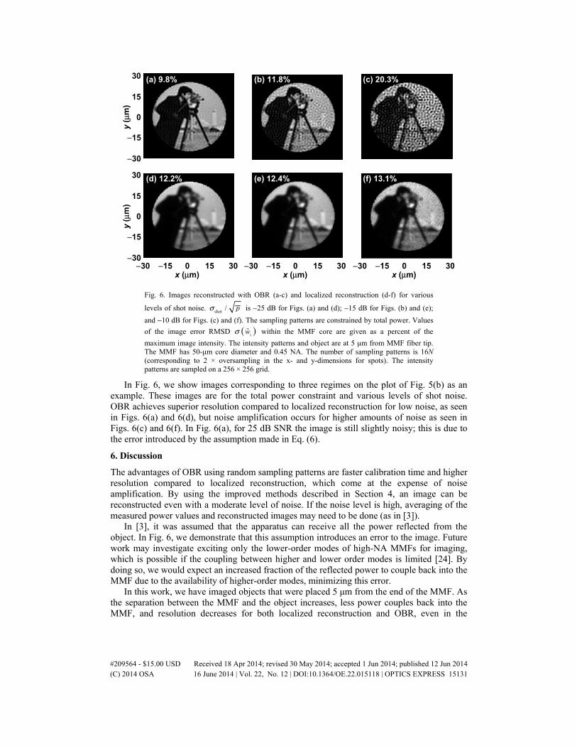
Fig. 6. Images reconstructed with OBR (a-c) and localized reconstruction (d-f) for various

levels of shot noise. shot / pσ is −25 dB for Figs. (a) and (d); −15 dB for Figs. (b) and (e);

and −10 dB for Figs. (c) and (f). The sampling patterns are constrained by total power. Values

of the image error RMSD ( )iwσ within the MMF core are given as a percent of the

maximum image intensity. The intensity patterns and object are at 5 μm from MMF fiber tip. The MMF has 50-μm core diameter and 0.45 NA. The number of sampling patterns is 16N (corresponding to 2 × oversampling in the x- and y-dimensions for spots). The intensity patterns are sampled on a 256 × 256 grid.

In Fig. 6, we show images corresponding to three regimes on the plot of Fig. 5(b) as an example. These images are for the total power constraint and various levels of shot noise. OBR achieves superior resolution compared to localized reconstruction for low noise, as seen in Figs. 6(a) and 6(d), but noise amplification occurs for higher amounts of noise as seen in Figs. 6(c) and 6(f). In Fig. 6(a), for 25 dB SNR the image is still slightly noisy; this is due to the error introduced by the assumption made in Eq. (6).

6. Discussion

The advantages of OBR using random sampling patterns are faster calibration time and higher resolution compared to localized reconstruction, which come at the expense of noise amplification. By using the improved methods described in Section 4, an image can be reconstructed even with a moderate level of noise. If the noise level is high, averaging of the measured power values and reconstructed images may need to be done (as in [3]).

In [3], it was assumed that the apparatus can receive all the power reflected from the object. In Fig. 6, we demonstrate that this assumption introduces an error to the image. Future work may investigate exciting only the lower-order modes of high-NA MMFs for imaging, which is possible if the coupling between higher and lower order modes is limited [24]. By doing so, we would expect an increased fraction of the reflected power to couple back into the MMF due to the availability of higher-order modes, minimizing this error.

In this work, we have imaged objects that were placed 5 μm from the end of the MMF. As the separation between the MMF and the object increases, less power couples back into the MMF, and resolution decreases for both localized reconstruction and OBR, even in the


absence of noise. For a MMF with larger core radius (but smaller NA such that the total number of modes is preserved), this distance increases.

7. Conclusion

We have quantified the noise amplification for the optimization-based multi-mode fiber endoscopic imaging method originally described in [3], and described three improvements to reduce noise amplification. A comparison of images obtained using noise-reduced OBR and the original OBR yielded a 20% reduction in image error for the noiseless case, and a further 33% reduction in image error at 22 dB SNR for the shot noise-limited case. As a comparison, we simulated imaging an object using both OBR and localized reconstruction under two constraints: on the maximum irradiance or on the total power of the sampling patterns. When imaging using random sampling patterns under the maximum irradiance constraint, we found that the image error using OBR was less than that of localized reconstruction for all SNRs when thermal noise-limited, and down to 18 dB and 19 dB SNR for shot and intensity noise-limited cases, respectively. When using spot sampling patterns under the total power constraint, we found that the image error using OBR was less than that of localized reconstruction for SNRs down to 15 dB, 15 dB and 16 dB for thermal, shot and intensity noise-limited cases, respectively.

Acknowledgments

Support from the Samsung GRO Program is gratefully acknowledged.


Documents

Noise-reduction algorithms for optimization- based imaging through