Noise optimisation in RC-activefilter sections

A.B. Haase and L.T. Bruton

Indexing terms: Active filters, Circuit computer-aided design, Noise, Optimisation, Transfer functions

Abstract: The paper is concerned with the noise optimisation of filter sections. A systematic approach basedon optimisation theory is taken, which makes use of the remaining freedom of choice of element valueswhen the transfer-function coefficients are fixed. An algebraic and a computer-aided noise optimisation aredescribed.

1 Introduction

One of the performance limitations of RC-active filters isthe generation of electrical noise within the filter which isadded to the signal to be processed. The noise performanceof active filters is investigated by, for example, References1 to 6. References 2 and 6 indicate ways leading to animprovement of the noise performance. References 7 and 8describe methods for cascading of sections which give anoptimum dynamic range. This paper is concerned with thenoise optimisation of filter sections. A systematic approachbased on optimisation theory is taken which makes use ofthe remaining freedom of choice of element values whenthe transfer-function coefficients are fixed. An algebraicand a computer-aided noise optimisation are described.

Fig. 1 Block diagram of general RC-active filter

2 Problem description

The class of RC-adive filters considered in this paper con-tains capacitances, resistances and differential-input single-ended output operational amplifiers (op-amps) as shown inFig. 1.

The noise generated within active filters results fromresistor thermal noise and active device noise. The noisesources shown in Fig. 1 represent the random fluctuationsof voltages and currents which are imposed on signals pro-cessed by the filter. The Johnson noise9 generated by re-sistors is described by the Nyquist formula.10 The 3-

Paper T60K, first received 23rd November 1976 and in revised form1st March 1977Dr. Haase is with Sefel Associates Ltd., 500 Bow Valley Square 11,Box 9088 Calgary Alb., Canada T29 2W4. Prof. Bruton is with theDepartment of Electrical Engineering University of Calgary,Calgary, Alb., Canada

generator noise model first mentioned in a Philbrick/Nexusmanual11 is employed for the op-amps. There are severalways to evaluate and compare the noise performance offilter networks.

2.1 Output noise power spectral-density function

The power spectral-density function (p.s.d.) of a noise vol-tage en or a noise current /„ describes the general frequencycomposition of en and in in terms of the spectral density oftheir mean square values t//2,

N(f) = lim, A/)

A/ (1)

Hence, the p.s.d. is a measure of i//2, at a particular fre-quency.12 Each noise source in Fig. 1 causes a noise voltageenok a t the output port, the p.s.d. of which is given by

Nok{f) = Nk(f)\1Xf)\2 (2)

where T(f) is the voltage transfer function Hnk2(f) from anoise voltage enk to the output port or the transimpedanceZnkiif) from a noise current ink to the output port. TheJohnson noise sources are statistically uncorrelated.Treleaven2 has shown that the correlation between thenoise sources en, inp and /„„ of the op-amp noise model isnegligible. This imples that the p.s.d. of the total outputnoise voltage eno is given by the sum of the output powerspectra calculated by assuming only one source at a time13

kk

No(f) = I Noktf) (3)

2.2 Total noise power at the output

The total output noise power Pn, which is the mean-squarevalue of the output noise voltage eno, is given by the areaunder the power spectral density function No (Reference 13)

= JNo(f)df (4)

The term power for Pn is accurate only in the sense that a1 fi load resistor is implied. Eqn. 4 leads to a finite valuefor Pn only if

(0 No(f) has a high frequency roll-off(ii) No(f) does not have 1//terms.

A nonzero value is chosen for the lower frequency limit ofeqn. 4 because the op-amp noise sources have a ]//depen-dence at low frequencies.2

ELECTRONIC CIRCUITS AND SYSTEMS, JUL Y 1977, Vol. I, No. 4 117

2.3 Signal/noise ratio

The signal/noise ratio (s.n.r.) is a measure of the purity of asignal and is simply the ratio of signal power Ps to noisepower Pn (see Reference 14)

s.n.r. = (5)

The signal power at the filter output is determined by theinput signal and the filter transfer function.

2.4 Dynamic range

For any filter network at a particular frequency, there is amaximum signal level that can be processed without ex-ceeding a tolerable level of signal distortion. There is also aminimum signal level which, in the following, is assumed tobe the noise level of the filter. The ratio between the as-sumed maximum and minimum levels is the dynamic range(d.r.).15 D.R. is defined to be

d.r. = Vosm \Hn{f)\\Hxa-mUn\\fK

(6)

where \Hia.max(f)\ is the maximum of the set of transferfunctions \HXam{f)\ from the filter input to the m op-ampoutputs, Vosm is the maximum permissible voltage swing atthe op-amp outputs and Hn(f) is the input-output transferfunction of the filter. The term \fPnl\HX2{f)\ is the noiselevel referred to the input and the term Vosml\Hla.max(f)\is the input voltage for which the maximum tolerable op-amp voltage swing is attained. Hl2(s) of the filter in Fig. 1is given by

pp

Hl2(s) = KQQ

= f(s,cp,dQ) = f(s,Q,Rj)(7)

Clearly, Hl2(s) depends upon the complex frequency s andthe transfer function coefficients cp, dq which, in turn, aredetermined by C, and Rj. For a given topology, and for pre-scribed values of cp and dq, there is not, generally, a uniquevalue for each element C, and Rj but a set of possible sol-utions leading to the same transfer function. This freedomof choice is utilised in the following to improve the noiseperformance of filters obtained by standard design pro-cedures.

3 Algebraic problem solution

To perform an optimisation, an objective function (o.f.) isrequired. This objective function indicates how the noiseperformance responds to variations of such parameters asKC-element values. The o.f. is subject to constraints such asthe maximum and minimum values of /?C-elements. Theseare represented by inequality constraints. The prescribedtransfer-function coefficients cp and dq are represented byequality constraints. An optimisation algorithm is appliedto the o.f. in order to answer the question as to what com-bination of the /?C-element values leads to an optimumnoise performance. Optimising the output noise power, thesignal/noise ratio and the dynamic range leads to two orthree different optima for most filter-synthesis techniqueswhich means that Pn, s.n.r. and d.r. have to be treated dif-ferently. Only the optimisation of Pn is described in the fol-lowing, for details of s.n.r. and d.r., see Reference 16.

118

The appropriate objective function is derived from eqns.3 and 4

kk

k = \

kk

= f(enk,ink,Ci,Rj)

(8)

In general, kk is equal to the number of noise sources in thefilter.

3.1 Optimisation strategy

The objective is to optimise a function o.f. of n variables xy

where these are the network /?C-element values. Each RC-element value is subjected to two inequality constraints ht

which define the RC-dement value range. While the vari-ables xy are being modified, it is necessary to maintain aconstant input-output transfer function. This is ensured bym equality constraints gj derived from the transfer functioncoefficients cp and dq

optimise o.f.(xy) y = 1 . . . n

subject to h{ > xymin i = 1 . . . n

hi<xymax i = n + 1 . . . 2/7

gj = 0 / = 1 m

(9)

This optimisation problem can be regarded as an n-dimensional box defined by the minimum and maximumvalues of the variables.

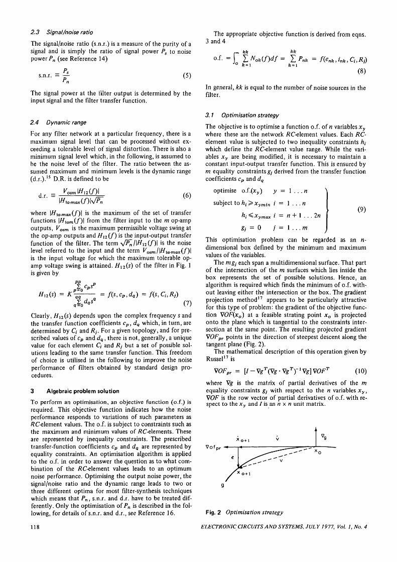
The mgj each span a multidimensional surface. That partof the intersection of the m surfaces which lies inside thebox represents the set of possible solutions. Hence, analgorithm is required which finds the minimum of o.f. with-out leaving either the intersection or the box. The gradientprojection method17 appears to be particularly attractivefor this type of problem: the gradient of the objective func-tion V0F(xo) at a feasible strating point xo is projectedonto the plane which is tangential to the constraints inter-section at the same point. The resulting projected gradientVOFpr points in the direction of steepest descent along thetangent plane (Fig. 2).

The mathematical description of this operation given byRussel17 is

TylVOFpr = [/-Vr(Vs-VsT'VslVOF (10)

where Vg is the matrix of partial derivatives of the mequality constraints gj with respect to the n variables xy,WOF is the row vector of partial derivatives of o.f. with re-spect to the xy and / is an n x n unit matrix.

Fig. 2 Optimisation strategy

ELECTRONIC CIRCUITS AND SYSTEMS, JULY 1977, Vol. 1, No. 4

Eqn. 10 gives only the search direction, no informationis available as to what the step magnitude a in that directionshould be. For the filter noise problem there is always atleast one nonlinear gy. This means that the direction givenby eqn. 10 leads away from the constraint intersection.Clearly, a controls the magnitude of the departure E fromthe intersection. Prescribing the maximum departure fromany gj and utilising a Taylor series expansion of gj, leads to

002ncp (ordQ)

VOFprHgjVOFfr(11)

for an n percentage error in cp (or dq). The worst departurein any of the cp (or dQ) is adjusted to n by applying eqn. 11to the mgj and determing the smallest a/n

j = 1 . . . m

A new point i"0 +1 is then calculated from

oc = min ocjn (12)

(13)

VOFpr always points in the direction of lower values of o.f.but a can overshoot the minimum because it is derivedfrom constraint information only. The minimum is thenlocated by a unidirectional search along VOFpr which leadsto a smaller a. The vector 0 pointing from x0 to jc0 + 1

leaves the constraint intersection by an error vector E . Forsmall a. the new point iro + i is close to the intersection, E,and hence the gj, are corrected to zero magnitude by em-ploying the normal Vg to the intersection and an approx-imation to the m-dimensional Newton method17

(14)

j3b is a column vector of m correction coefficients and g isthe column vector of the mgj. The iteration equation (eqn.14) is repeated until a fo+i is found which reduces themagnitude of the largest departure from any cp or dQ belowa prescribed error limit. The corrected new point * 0 + i isthen calculated from

This, then, is the starting point for the next iteration of x;the above procedure is repeated with new points xx+1 re-placing old points xx until the minimum of o.f. is reached.Each optimisation step results in a vector v pointing fromxx to a new location xx + l where o.f. assumes a lower valueif a is properly chosen. In general, the resulting vector veventually leaves the box defined by minimum and maxi-mum element values, thus violating at least one of the in-equality constraints /*,- (see eqn. 9) and placing xx + j in aforbidden region. In this case v is shortened by adjustingthe step magnitude a such that xx +1 lies right on the bound-ary, and the corresponding variables xy are held constant ateach successive iteration.

The optimisation of o.f. is terminated when the improve-ment by an additional step is below a preset limit. Lagrangemultipliers17 can be employed to check if a minimum isreached, or the termination is caused by a region of slowconvergence.

4 Computer-aided problem solution

In Section 2 the procedure for the determination of thefilter output noise is found to involve the calculation of thetransfer functions |//,o(/co)|2 from each resistor Rj and

every noise generator of the op-amp noise model in Fig. 1to the output port. In general, these transfer functions aredifferent from each other, and of order equal to that of theinput-output transfer function, which leads to complicatedcalculations even for fairly simple filters. Moreover, eqn. 8for the o.f. shows that an integration of the weighted sumof the \HiO(jw)\2 is required. Clearly, a problem of thiscomplexity requires the aid of a computer.

The optimisation procedure described in Section 2 iseasily programmed for the use of digital computers. Variousother routines are available; however, existing optimisationroutines that allow nonlinear constraints are based ongeneral algebraic methods which are wasteful for the specificproblem of noise optimisation in active filters. The dis-advantage of the above approach is the necessity for analgebraic equation that would represent the total outputnoise power Pn. It is highly desirable to delegate the lengthycalculation of noise transfer functions and p.s.d. integrationto the computer. The approach taken is therefore to linkthe optimisation algorithm of Section 3 with a suitablenetwork-analysis routine. This eliminates the need to formu-late the optimisation problem in terms of a complicatedobjective function. The analysis routine is based upon thenullor concept18 and the standard branch approach.19 Anodal admittance matrix is set up from topology infor-mation, and the complex voltages at all network nodes arecomputed for all network sources independently and simul-taneously. The noise transfer functions are derived from thecomputed node voltages and utilised for the computationof the total output noise power spectral-density functionNo(f) according to eqns. 2 and 3. The total output noisepower Pn, and, hence o.f., is computed from No(f) bynumerical integration employing the trapezoidal rule,thereby approximating eqn. 4.

VOF is computed utilising network sensitivities(i) The sensitivity S" of a filter transfer function H with

respect to an element x is equal to the fractional change inH divided by the fractional change in x, assuming that allchanges are incremental20

«Jy = —— Z — (16)H bx 3 (In*) H Ax

Expressing H in polar co-ordinates gives for the derivative

(17)dx Ax

Fig. 3 General filter network for sensitivity calculation

ELECTRONIC CIRCUITS AND SYSTEMS, JULY 1977, Vol. l.No. 4 119

(ii)Geher21 has shown that Sx can be calculated as

(18)

where Vc and Vx are the voltages at the filter output and atthe element x, respectively, caused by an input voltage Va

and Hbo is the transfer function from a voltage Vb (in serieswith the element x) to the output port. Fig. 3 shows thecorresponding general network.

(iii) In general, perturbing an element x alters the noisetransfer functions and transimpedances Tk2 between the knoise sources and the output port. Hence, a departure of Pn

and therefore o.f. results. For example, from eqn. 17 theerror of \VC\ in Fig. 3 due to a small fractional change Ax/xin JC is found to be

A\VC\~\VC

Observing that for incremental changes

(19)

(20)

the perturbed output noise p.s.d. is calculated as

No(f, x + Ax) =*No(f, x) + 2 — J> o f e Re | ^ * 2

= No(f) + ANo(f) (21)

where T^x is the transfer function or transimpedance be-tween the k'ih noise source and the network branch con-taining the element x under consideration and Hx2 is thetransfer function between this branch and the output port.The perturbed output noise power Pn(x + Ax) is foundby numerical integration of eqn. 21. Then VPn = VOF isapproximated by a finite-difference method:

(22)Ax

Thus, the required derivatives can be computed from thenode voltages provided each optimisation variable is com-bined with a voltage source Vb. Additional voltage sourcesare required only for capacitors because the networkbranches of resistive variables already contain Johnsonnoise generators which can be employed for the sensitivitycomputations (caution: perturbing a resistor should perturbthe corresponding Johnson noise generator).

The equations for the equality constraints, i.e. the trans-fer function coefficients, and their first partial derivativeswith respect to the variable network elements are to be pro-vided. The second partial derivatives are computed therefrom by a finite-difference method. Furthermore, the im-provement limit for o.f. is to be specified below which thealgorithm is to be terminated.

5 Numerical example

The two integrator loop22 shown in Fig. 4 is used as an ex-ample. The element values given in Fig. 4 realise a 3rd-orderButterworth low-pass filter with a cut-off frequency of1 kHz, and are calculated following the design proceduresuggested by Kerwin et al.22

The input-output transfer function of Fig. 4 is

K

+s2d2)(\ +sCnRn)

where

K =

fj — ^8^10 —

d2 —R<

(23)

(24)

(25)

(26)

The transfer functions fromoutput port are

HRI = Hn

HR2 = R±H

R2

RA,

R 4 ~ (1 +

HRS =

HR3

HR6 = (1 +

1 +sdx +s2d

1

sdi +s2d2)(\

sC7R5)HR3

the resistors in Fig.

1

2)(l+sC

+ sCnR

12^11)

11)

4 to the.

(27)

(28)

(29)

(30)

(31)

(32)

(33)

Fig. 4 Two integrator loop example

t o o120 ELECTRONIC CIRCUITS AND SYSTEMS, JULY 1977, Vol. 1, No. 4

HDQ — HiR2

s2d2)(l+Cl2Rn)(34)

The transfer functions from the op-amp voltage noisesources to the output port are

x +s2d2)(\+CnRn)

Hnv2 = HR6

(35)

(36)

(37)

For the op-amp current noise sources it is found that thetransimpedances are given by

7 - R H (381

7 = /?o//D, (391^nn\ •*»3-r*.R3 v J ^ /

7 - R.Hn. C40)

Z = R H (41)

Znn3 = R&HR% (43)

The p.s.d. of the Johnson noise generators in resistors isgiven by10

V2

7Vr = 4kTR =* 1 -6 x 10"20 R —— (44)S2 Hz

The p.s.d.s of the op-amp noise generators are taken fromBruton and Treleaven5

N white = 9x 10"16V2/Hz

^IM/HIHZ = 2-62 x 10"14V2/Hz

tyn 11 HZ = 2-21 x 10"23A2/Hz

JV.pl!HZ = 4-49 x 10"23A2/Hz

(45)

(46)

(47)

(48)

The lower limit on the integration (eqn. 8) is chosen to be1 Hz. Frequencies below 1 Hz are considered to be d.c.drift.3- "

The permissible minimum and maximum element values,which are required for the optimisation and represent theelement spread, are assumed to be

l n F < C < 1 0 0 n F (49)

(50)

The noise optimisation can be simplified by observing thatthe time constant Cl2Rn is fixed by the prescribed transferfunction. From eqn. 44 it is clear that the smallest noisecontribution by Rn is achieved when Ru assumes thesmallest possible value.

Furthermore, the d.c. offset compensating resistors R6

and R9 in the noninverting inputs of the integrator op-ampsare assumed to equal the ohmic resistance to earth seen bythe corresponding inverting inputs, i.e.

Rg =

(51)

(52)

Hence, there remain eight variables and two equality con-straints for the optimisation. The latter are derived fromthe invariant transfer-function coefficients dx and d2 ineqns. 25 and 26 and the element values given in Fig. 4

f. = C..K. j - 1.592 x 10-" = 0 (53)

g2 = C7JRsC10/?8 ^ -2-533 x 10"8 = 0 (54)

Introducing the above numerical values and equations intoeqn. 8 and performing the integration leads to

pn = o.f. = 2-621 x 10"12 + 1-676 x lO"1 7/^

+ 1-563 x \0~22Rl + 2-513 x 10~17tf8

+ 6-734 x 10"23/?l + 2-256 x \0~12R^/R3

+ l-676x \0~llRl/R3

+ (RJR3)2(2-256 x 10"12

+ 3-351 x 10"17/?5 + 4-738 x 10~227?i)

+ C3/?!^f (3-876 x 10"5

^ 3

+ 3-307 x \0~10R5 + 1-329 x \0~l5R25

+ 6-615 x 10"10/?8 + 1-983 x \0~l5Rl)

(1-128 x 10,-12

(/?, +R2)2Rl

+ 1-676 x 10"17/?2 + 3176 x 10"22R\

+ 3-351 x 10"17/?8 + 4-738 x 10"22/?l)

Table 1

Step

012345678

10k8-6476-6624-9524 0943-6143-2493 0842-718

kft10k11-12213-21315-6771704517-47917-49214-54011 -449

* 3

kn10k13-77318-7022429428-99232-82536-37940-38749-901

k n10k60143-6662-4091-8831-5101-28010211021

kft10k11 -84713-94515-72717-25918-76020-29024-90228-175

kft10k12-36314-67615-9411447611 -9709-8118-8738-131

nF15-916n19-33523-34026-928300253304536-16615-33954037

nF15-916n20-4822704537-83653-37474-175

100 0010000100 00

Pn

11 2435-93142413-6403-3853-3223-1063 0643 043

ELECTRONIC CIRCUITS AND SYSTEMS, JULY 1977, Vol. 1, No. 4 121

where the straight-line approximation of the Bode plot ofthe corresponding transfer functions is used for frequency-dependent noise sources. The required derivatives of o.f.and g, which are VOF, Vg and Hg, are calculated in astraightforward manner from eqns. 53 to 55.

For a step magnitude a. corresponding to a 10% error indx and/or d2 Table 1 shows the result of eight subsequentoptimisation steps. Step 6 leads to a boundary which is themaximum value of Cx0. Therefore C10 remains at 100 nFfor the steps beyond step 6 and the corresponding deriva-tives are zero. The minimum Pn is within 16-1% of thenoise floor where the noise floor is the first r.h.s. term ofeqn. 55.

The computer-aided approach described in Section 4leads to a minimum o(Pn of 2-986juV£ns. The difference toTable 1 is caused by a relative coarse-frequency grid usedfor the numerical integration ofN0(f).

Rc=80K

Fig. 5 F.D.N.R. ladder filter example

Fig. 6 G.I.C. biquad example

6 Conclusions

The 3rd-order Butterworth lowpass filter with/c = 1 kHz, asemployed in Section 5, is utilised to compare the noise per-formance of various synthesis techniques

(i) F.D.N.R.-ladder filter22 (see Fig. 5)The g.i.c. suggested by Antoniou24 is employed to simulatethe f.d.n.r. The low-frequency roll off is compensated forutilising the technique described by Bruton et al.2s The im-pedance level is kept constant.

(ii) G.I.C. biquad26 (seeFig. 6)The same g.i.c. as under (i) is employed.24 The elements ofthe circuit given by Reference 26 are selected as follows:

Yl = Gx = ^-(Rx =

Y2 = sC2(C2 = 31-83nF)

Y3 = 0

= 5kH,C4r 4 = G4 + sC4 = — +sC4

= 15-92 nF)

Ya = sCa(Ca = 15-92nF)

Yb= —(Rb = lOkH)Kb

Y = Y1 c I a

Yd ~ Yb

(iii) Two integrator loop22 (see Fig. 4)

(iv) Sallen-Key circuit no. I21 (see Fig. 7)

Fig. 7 Sallen-Key filter example

Table 2

Synthesis technique r.m.s.-noise S.N.R. D.R.

F.D.N.R. ladderG.I.C. biquadTwo integrator loopSallen-Key no. 1Bach

20012-5981-7441-9642-188

0-624 X1 -482 X4-818 X2-600 X2-089 X

10'10'10s

10'10'

1 -202 X1-196 X2-289 X3-601 X2-285 X

10*10*10*10*10*

Table 3: Element values of f.d.n.r. ladder example

Standard designPn optimum ands.n.r. optimumd.r. optimum

nF31-83

2-75

21-36

* 3

kn50004649

6712

nF31-8331-83

44-47

kn5000

12683

4202

kft50001000

5289

122 ELECTRONIC CIRCUITS AND SYSTEMS, JUL Y 1977, Vol. 1, No. 4

Table 4: Element values of g.i.c. biquad example

Standard design Pn optimumS.N.R. optimum

D.R. optimum

Ca, nFRb,kO.CC/nFRd, kJ2

C2'.'nFC«,nF

15-9210015-9210010031-8315-9250

3-4710-9717-8833 024-57

69-6139-2203

57-913-32

61-9610503

63-3367-37

1-18

Table 5: Element values of two integrator loop example

Standarddesign

Pn optimum S.N.R.optimum

D.R.optimum

R. , kSlR2, kJ2/?,, kn.R4, k£lRs, kSlR6. kfZC,,nF/?8, kSlR , kflCl0,nF/?,,, kfi

1 0 01 0 010010010010015-921 0 01 0 015-921 0 015-92

2-7211-4549-9

1 0 228-1828-1854 08-138-13

10001-59

1000

1 033:544-299-431-421-424-73

21-8521-8578-60

1-591000

1 01 01 01 01-591-59

100001-591-59

100 01-59

1000

C2= 15-92 nF

Fig. 8 Bach filter example

E;>"a.a5SIO

c

rms.

6

•4

2fl

I IinO

5:zI/)

-6

-4

•2

.ill

O

cta

•

1

-3

-2

-1

a b o d e a b o d e a b o d e

Fig. 9 Comparison of noise performance of 3rd-orderButterworth lowpass examples

Q = standard design •a F.D.N.R. ladderb G.I.C. biquadc Two integrator loop

= optimised designd Sallen-Keye Bach

(v) 2nd-order Bach circuit2* (see Fig. 8)The element-value ranges chosen for the optimisation aregiven by eqns. 49 and 50. The calculated optimum noiseperformance characteristics, that is the minimum outputnoise power (Pn), the maximum signal/noise ratio (s.n.r.)and the maximum dynamic range (d.r.), are given in Table 2and Fig. 9. Note that the maximum d.r. can differ from the

maximum s.n.r. because an additional constraint, the maxi-mum signal level, is used for the optimisation of d.r. S.N.R.is calculated for a 1 mV r.m.s. passband input signal, amaximum op-amp output voltage of 10 V r.m.s. is assumedfor the calculation of d.r. Tables 3—7 show the elementvalues of the optimised circuits. The calculations show thatthe optima are fairly insensitive to small element valuechanges. Thus, standard resistor and capacitor values maybe used without great departure from these optima. Table 2shows that the two integrator loop offers the best r.m.s.noise and s.n.r. performance even though this is the struc-ture with the largest number of op-amps and elements. Theselected values of the op-amp noise generators in eqns. 45to 48 that have been used for the above comparison aretypical for the widely used type-741 op-amp. It is foundthat the op-amp voltage noise predominates over the othernoise contributions. The 1//noise contributions are smallin comparison with other noise contributions for the fre-quency range and impedance level considered. The errorincurred by applying the straight-line approximation istherefore negligible. In conclusion, optimisation results insome improvement of the considered performance par-ameters, though in some cases by a rather small amount.

Table 6: Element values of Sallen-Key example

Standard design Pn optimum andd.r. optimum

S.N.R. optimum

fix.c2.« 3 -

R\'.

kf inFkftnFkf ik f iknnF

1 0 015-921 0 015-9210010010015-92

1-81100 0

12-8710-89

short circuitopen circuit

1-59100 0

1-52100 0

11 0415062-14

10-891-59

1000

Table 7: Element values of Bach example

Standard design Pn optimum and s.n.r. optimumand d.r. optimum

RltknC2,nFR3, knC4'nFR , kJ2C6'nF

1 0 015-921 0 015-921 0 015-92

7 References

1-59100 0

1-59100 0

1-59100 0

1 TROF1MENKOFF, F.N., BRUTON, L.T., and SMALLWOOD,R.E.: 'Noise analysis of 4th order maximally-flat bandpass filter'.Record of the National Electronics Conference, Chicago, 1972,pp. 223-227

2 TRELEAVEN, D.H.: 'Electrical noise in inductorless filters',Ph. D. dissertation, University of Calgary, 1972

3 TROFIMENKOFF, F.N., TRELEAVEN, D.H., and BRUTON,L.T., 'Noise performance of /?C-active quadratic filter sections',IEEE Trans., 1973, CT-20, pp. 524-532

4 BRUTON, L.T., TROFIMENKOFF, F.N., and TRELEAVEN,D.H.: 'Noise performance of low sensitivity active filters', IEEEJ. Solid-State Circuits, 1973, SC-8,pp. 85-91

5 BRUTON, L.T., and TRELEAVEN, D.H.: 'Electrical noise inlowpass FDNR-filters', IEEE Trans. 1973 CT-20, pp. 154-158

6 ZURADA, J., and BIALKO, M.: 'Noise and dynamic range ofactive filters with OPAMPs'. Proceedings 1974 IEEE Inter-national Symposium on Circuits and Systems, pp. 677-681

7 NOVAK, M.: 'Optimisation of dynamic ratio by active RCfilters'. Proceedings 1974 IEEE International Symposium onCircuits and Systems, pp. 635-639

ELECTRONIC CIRCUITS AND SYSTEMS, JUL Y 1977, Vol. 1, No. 4 123

8 LUEDER, E.: 'Optimisation of the dynamic range and the noisedistance of /?C-active filters by dynamic programming', Int. J.Circuit Theory & Appl, 1975, 3, pp. 365-370

9 JOHNSON, J.B.: 'Thermal agitation of electricity in conductors',Phys. Rev. 1928, 32, pp. 97-109

10 NYQU1ST, H.: 'Thermal agitation of electric charge in conduc-tors', ibid., 1928, 32, pp. 110-113

11 Applications manual for computing amplifiers (Philbrick/NexusResearch, Mass, USA, 1965)

12 BKNDAT, J.S., and P1ERSOL, A.G.: 'Random data: analysis andmeasurement procedures' (Wiley-lnterscience, 1971)

13 LATHI, B.P., 'Communication systems' (John Wiley 1968)14 TAUB, H., and SCHILLING' D.L.: 'Principles of communication

systems' (McGraw-Hill, 1971)15 ORCHARD, H.J., and SHEAHAN, D.F.: inductorless bandpass

filters', IEEEJ. Solid-State Circuits, 1970, SC-5, pp. 108-11816 HAASE, A.B.: 'Noise and distortion in RC-activc filters', Ph.D.

dissertation, University of Calgary, 197517 RUSSEL, D.L.: 'Optimisation theory' (W.A. Benjamin Inc.,

1970) Chaps. 4 and 918 DA VIES, A.C.: 'The significance of nullators, norators and

nullors in active-network theory', Radio & Electron Eng., 1967,34, pp. 259-267

19 COLDHAM, D.B., and BURTON, L.T.: 'Computer analysis of

nullor networks', Electron. Lett., 1973, 9, pp. 80- 8220 BODE, H.W.: 'Network analysis and feedback amplifier design',

Van Nostrand 1945)21 G^HER, K.: 'Theory of network tolerances, (Akademiai Kiado,

Budapest, Hungary, 1971)22 KERWIN, W.J., HUELSMAN, L.P., and NEWCOMB, R.W.:

'State-variable synthesis for insensitive integrated circuit transfer-functions', IEEE J. Solid-State Circuits, 1967, SC-2, pp.87-92

23 BRUTON, L.T.: 'Network transfer-functions using the conceptof frequency dependent negative resistors'. IEEE Trans., 1969CT-16, pp. 406-408

24 ANTONIOU, A.: 'Realisation of gyrators using operationalamplifiers and their use in /?C-active-network synthesis', Proc.IEE, 1969, 116, (11), pp. 1838-1850

25 BRUTON, L.T., PEDERSON, R.T., and TRELEAVEN, D.H.:'Low-frequency compensation of FDNR lowpass filters', Proc.IEEE, 1972, 60, pp. 444-445

26 BRUTON, L.T.: 'Biquadratic sections using generalized im-pedance converters', Radio and Electron. Eng., 1971, 41, pp.510-512

27 SALLEN, R.P., and KEY, E.L.: 'A practical method of designingRC-active filters',//?if Trans., 1955, CT-2, 74-85

28 BACH, R.E.: Jun., 'Selecting flC-values for active filters',Electron., 1960, 33, pp. 82-85

George S. Moschytz received the M.S.and Ph.D. degrees in electrical engin-eering from the Swiss Federal Instituteof Technology, Zurich, Switzerland, in1958 and 1960, respectively. From1960 to 1962 he was with the RCALaboratories Ltd., Zurich, where heworked on colour t.v. signal trans-mission problems, and, in particular, onnew and high-precision methods of

|envelope delay measurement in video-transmission systems. In 1963 he joined Bell TelephoneLaboratories, Inc. Holmdel, N.J., where, as Supervisor ofthe Active Filter Group in the Data Communications Lab-oratory, he investigated methods of synthesising hybrid-integrated linear and digital circuits for use in data trans-mission equipment. This work inlcuded the design of activeRC data modems and filter schemes suitable for implemen-tation with thin-film and silicon-integrated-circuit elements.From 1972 to 1973 he was on a leave of absence from BellLaboratories and Visiting Professor at the Swiss FederalInstitute of Technology. Since 1973 he has been Professorof Electrical Engineering and Director of the Institute ofTelecommunications at the Swiss Federal Institute ofTechnology.

Prof. Moschytz has written two books and numerouspapers in the fields of active network theory, design andsensitivity. Prof. Moschytz is a member of the Swiss Elec-trotechnical Society and a senior member of the IEEE.

Peter Horn was born in Czechoslovakia,on 31st July 1946. He received theM.S. degree in electrical engineeringfrom the Swiss Federal Institute ofTechnology, Zurich, in 1972, where heis now at the Institute of Telecom-munications as a research assistant.

124 ELECTRONIC CIRCUITS AND SYSTEMS, JUL Y 1977, Vol. 1, No. 4