Noise-Optimal Capture for High Dynamic Range Photography

Samuel W. Hasinoff Fredo Durand William T. FreemanMassachusetts Institute of Technology

Computer Science and Artificial Intelligence Laboratory

Abstract

Taking multiple exposures is a well-established approach

both for capturing high dynamic range (HDR) scenes and

for noise reduction. But what is the optimal set of photos

to capture? The typical approach to HDR capture uses a

set of photos with geometrically-spaced exposure times, at

a fixed ISO setting (typically ISO 100 or 200). By contrast,

we show that the capture sequence with optimal worst-case

performance, in general, uses much higher and variable

ISO settings, and spends longer capturing the dark parts of

the scene. Based on a detailed model of noise, we show that

optimal capture can be formulated as a mixed integer pro-

gramming problem. Compared to typical HDR capture, our

method lets us achieve higher worst-case SNR in the same

capture time (for some cameras, up to 19 dB improvement

in the darkest regions), or much faster capture for the same

minimum acceptable level of SNR. Our experiments demon-

strate this advantage for both real and synthetic scenes.

1. Introduction

Taking multiple exposures is an effective solution to ex-

tend dynamic range and reduce noise in photographs. How-

ever, it raises a basic question: what should the set of expo-

sures be? Most users rely on a geometric progression where

the exposure times are spaced by factors of 2 or 4 with the

number of images set to cover the range. The camera sensi-

tivity (ISO) is usually fixed to the nominal value (typically

100 or 200) to minimize noise. Given that noise is the main

factor that limits dynamic range in the dark range of val-

ues, it is critical to understand how noise can be minimized

in high dynamic range (HDR) imaging. In this paper, we

undertake a systematic study of noise and reconstruction in

HDR imaging and compute the optimal exposure sequence

as a function of camera and scene characteristics.

We present a model that predicts signal-to-noise ratio at

all intensity levels and allows us to optimize the set of ex-

posures to minimize worst-case SNR given a time budget,

or to achieve a given minimum SNR in the fastest time. To

do this, we use a detailed model of camera noise that takes

into account photon noise, as well as additive noise before

and after the ISO gain. This allows us to optimize all pa-

rameters of an exposure sequence, and we show that this

reduces to solving a mixed integer programming problem.

In particular, we show that, contrary to suggested practice

(e.g., [5]), using high ISO values is desirable and can enable

significant gains in signal-to-noise ratio.

The most important feature of our noise model is its ex-

plicit decomposition of additive noise into pre- and post-

amplifier sources (Fig. 1), which constitutes the basis for

the high ISO advantage. The same model has been used

in several unpublished studies characterizing the noise per-

formance of digital SLR cameras [7, 20], supported by ex-

tensive empirical validation. Although all the components

in our model are well-established, previous treatments of

noise in the vision literature [13, 18] do not model the de-

pendence of noise on ISO setting (i.e., sensor gain).

To the best of our knowledge, varying the ISO setting

has not previously been exploited to optimize SNR for high

dynamic range capture. However, in the much simpler con-

text of single-shot photography, the expose to the right tech-

nique [25, 20] considers the ISO setting to optimize SNR.

This technique advocates using the lowest ISO setting pos-

sible, but increasing ISO when the exposure time is tightly

constrained. Another related idea is the dual-amplifier sen-

sor proposed by Martinec, which would capture exposures

at ISO 100 and 1600 simultaneously and then combine them

to extend dynamic range [20]. Our method can be thought

of as formalizing these ideas, generalizing them to a multi-

shot setting, and showing how to optimize the capture se-

quence for a given camera and scene.

Most previous work in HDR imaging has focused on

calibrating the response curve of the sensor [8, 22], merg-

ing the input images [16, 3], and tone mapping the merged

HDR result [17, 9]. Surprisingly little attention, however,

has been paid to the capture strategy itself, which is the fo-

cus of this paper. One notable exception is a method that

computes the optimal set of exposure times to reduce quan-

tization in the merged HDR result [10]. This works by ef-

fectively dithering the exposure levels, but assumes that ex-

posure times can be controlled arbitrarily, and does not in-

corporate a detailed model of noise. Another recent method

[4] showed how to minimize the number of photos span-

ning a given dynamic range, but takes a simplified geomet-

ric view of dynamic range, without any noise model.

exposuretime t

radiantpower from

scene ©

darkcurrent D

photonnoise

readoutnoise

gainfactor 1/g

quantizeddigital value I

ADCnoise

sensorsaturation

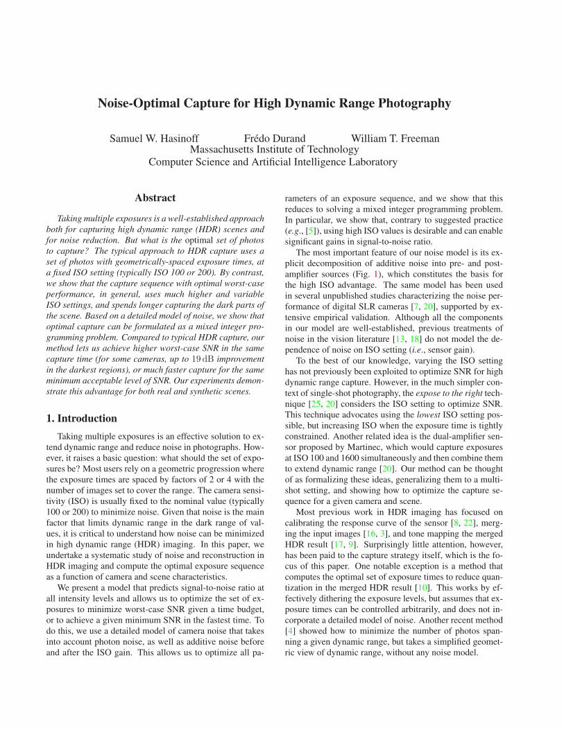
Figure 1. Imaging chain for a single pixel, from radiant power to raw pixel measurement. The components of our noise model are indicated

by dashed boxes (we defer treatment of dark noise to supplemental materials). Our goal is to recover Φ with maximum worst-case SNR

over the desired dynamic range, by determining an optimal sequence of photos to capture, with exposure times ti(k) and gain settings gj(k)(controlled by the shutter speed and ISO setting respectively).

Several recent digital cameras, such as the Sony A550

and the Pentax K7, offer in-camera HDR from several con-

secutive shots. The underlying settings that these cameras

use for HDR capture is unclear, but they do not appear to

take advantage of ISO setting the way our method does.

Our analysis is also related to “multiple capture” HDR

sensors, which address similar issues by taking multiple

readings of the accumulated charge within a single exposure

[19, 6]. Sensors of this kind typically take evenly spaced

readings over the exposure, and return the last sample be-

fore saturation, scaled by the saturation time. More recently,

an online weighting scheme was proposed to combine all

readings [19], analogous to merging techniques used in

standard HDR. Even closer to our method, the spacing of

these readings has been optimized to improve average SNR

[6]. But this method only models photon noise and does not

consider the possibility of manipulating gain.

Our method offers four contributions over the state of the

art. First, we show that by capturing high ISO images we

can improve worst-case SNR for HDR capture (up to 19 dBfor some cameras). Second, we show how to compute the

globally optimal capture sequence, maximizing worst-case

SNR or minimizing capture time, by solving a mixed in-

teger programming problem. Third, we describe a simple

HDR merging technique that takes sensor noise and ISO

into account and minimizes the variance of the estimate.

Fourth, our experiments with real scenes validate our pro-

posed method, and confirm its benefits for existing cameras.

2. Image Formation Model

By restricting our attention to the raw images captured

by the sensor, we simplify our analysis in two ways. First,

raw images let us consider each pixel independently, be-

cause they incorporate no additional processing, such as

demosaicking, that would introduce correlations.1 Second,

raw pixel values are linear in the radiant energy collected,

to a close approximation [7, 20].

Like nearly all methods for high dynamic range capture

[8, 22], we assume that aperture and focus are held con-

1Pixel independence may be violated by sensor bloom, but this type

of artifact is mainly affects lower-quality CCD sensors [13]. Systematic

per-pixel noise variations, such as fixed pattern noise and pixel response

non-uniformity, may be handled by pre-capture calibration [13, 20].

stant, to avoid changing defocus [11]. This leaves just two

camera settings to manipulate: (1) the exposure time, which

controls the amount of light collected, and (2) the ISO set-

ting, which controls the sensor gain.

Pixel measurement model. The quantity each pixel mea-

sures is the radiant power, Φ, of the light it collects (Fig. 1).

While we can loosely think of Φ as scene brightness, we

are not concerned with its relationship to absolute scene

irradiance—only its accurate measurement. In particular,

our analysis is independent of photometry [15], and of lens-

dependent effects such as vignetting and glare [24], all of

which can be calibrated separately.

For convenience we express Φ in units of electrons per

second, so that Φt photoelectrons are collected over an ex-

posure time of t seconds. For raw images, we can describe

the measured pixel value, I , given in digital numbers (DN)

[7], as a linear function of number of electrons collected:

I = min { Φt/g + I0 + n, Imax } (1)

where g is the sensor gain, with units of electrons per DN;

I0 is a constant offset representing the black point; n is the

signal- and gain-dependent sensor noise, described below;

and Imax is the saturation level. Sensor saturation occurs

when (Imax − I0)g electrons are collected, which is limited

by both the “full well” electron capacity and the gain.

One subtlety in Eq. (1) is that pixel values just below

Imax are ambiguous: such pixels may actually be saturated

but corrupted by negative post-saturation noise (Fig. 1). In

practice, we address this issue by using a more conservative

saturation level, Imax(g) < Imax, determined empirically

for each sensor gain as the minimum pixel value in a com-

pletely over-exposed image.

The sensor gain g and ISO setting G are inversely related

by G = U/g, where U is a camera-dependent constant.

Noise model. To model the essential properties of noise,

we treat noise as a zero-mean random variable, whose vari-

ance comes from three independent sources (Fig. 1). For

pixels below the saturation level, we can write:

Var(n) =

photon noise︷ ︸︸ ︷

Φt/g2 +

additive noise︷ ︸︸ ︷

σ2read/g

2

︸ ︷︷ ︸

pre-amplifier

+ σ2ADC

︸ ︷︷ ︸

post-amplifier

(2)

The first term represents the Poisson distribution of pho-

ton arrivals, and depends linearly on the number of photons

recorded, Φt. The final two terms decompose the scene-

independent noise variance into pre- and post-amplifier

components [7, 20]: the middle term represents noise from

sensor readout; the last term represents the combined effect

of analog-to-digital conversion (ADC), including amplifier

noise and quantization.2

For a fixed ISO setting, this model reduces to the well-

known affine model of noise that has been recently exploited

for image processing [18] and analysis of camera designs

[12, 26, 2]. The key difference in our analysis is that we

make explicit the dependence of additive noise on ISO set-

ting, and take advantage of this for HDR capture.

3. The High ISO Advantage

Our new approach to capturing HDR images takes ad-

vantage of a somewhat counter-intuitive fact: saturation

aside, photos with high ISO settings have higher SNR for

a given scene brightness and exposure time, particularly in

the darkest regions of the scene.

For single-shot photography, pixel saturation prevents

us from exploiting the high ISO advantage, except when

the dynamic range of the scene is small. However, as we

show, we can find sequences of photos for HDR capture that

achieve the SNR improvement associated with the highest

ISO settings, but still span the desired dynamic range.

The high ISO advantage follows directly from our im-

age formation model, and we explain it by characterizing

several factors affecting SNR.

SNR for a single shot. For a single exposure, we can

combine Eqs. (1) and (2) to compute the squared SNR for a

pixel, in terms of the measured radiant power Φ,

SNR(Φ)2 =Φ2t2 · [I < Imax(g)]

Φt+ σ2read + σ2

ADCg2

, (3)

where [I < Imax(g)] is a binary indicator modeling the fact

that SNR for saturated pixels is zero.

We graph SNR using the noise parameters of a real cam-

era in Fig. 2. Note that each graph has a shoulder at the

transition between the two main noise regimes. For dark

pixels, additive noise is dominant, so SNR increases with

Φ. For bright pixels, photon noise is dominant, so SNR in-

creases instead with√Φ.

SNR vs. saturation tradeoff. As Eq. (3) shows, SNR

increases monotonically with the number of electrons col-

lected, Φt, up to saturation. This property justifies the ex-

pose to the right principle [25, 20]: to maximize SNR in

2To simplify the presentation we collect all post-amplification noise

into a single term. Some cameras use a two-stage amplifier [20], but our

analysis applies to these cameras as well.

normalized exposure time equal exposure time

−12 −10 −8 −6 −4 −2 0−20

0

20

40

log2 (Φ / Φ

max)

SN

R (

dB

)

ISO 100

ISO 200

ISO 400

ISO 800

ISO 1600

ISO 3200

−12 −10 −8 −6 −4 −2 0−20

0

20

40

log2 (Φ / Φ

max)

SN

R (

dB

)

ISO 100

ISO 200

ISO 400

ISO 800

ISO 1600

ISO 3200

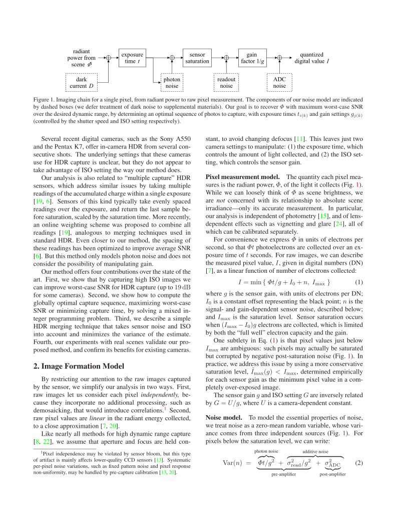
Figure 2. SNR for the Canon 1D Mark III, at various ISO settings,

as a function of the radiant power from the scene, Φ. Left: Ex-

posure time adjusted for each ISO to keep Φt/g constant (e.g., at

ISO 800, we expose for 1/8 the time as for ISO 100). In this set-

ting, higher ISOs record less electrons and so have lower SNR.

Right: Exposure time held constant, so that all ISOs record the

same number of electrons. Higher ISOs have higher SNR for a

given scene brightness, especially in the darkest parts of the scene,

but they also lead to earlier pixel saturation.

a single shot, we should choose exposure time to make

the highlights expose just below Imax. By contrast, a

naıve application of auto-exposure would expose a uniform-

brightness scene to only 0.13Imax [14].

More generally, choosing the exposure time for any

photo represents a tradeoff between SNR and pixel satura-

tion. The longer we expose an image, the higher the SNR.

But beyond the exposure time needed to expose right, SNR

improvements come at the expense of saturating the high-

lights. This tradeoff is particularly important for high ISOs,

because of their lower dynamic range (Fig. 2).

The high-ISO potential. As Fig. 2(right) illustrates, for

a fixed number of electrons collected, high ISO settings are

limited by sensor saturation, but have improved SNR for

the non-saturated parts of the scene. We can explain this

effect by the reduced influence of ADC noise at higher ISO

(Fig. 3). Since this noise comes after amplification, its vari-

ance in squared electrons, σ2ADCg

2, falls to zero with in-

creasing ISO (i.e., decreasing gain).

We call the SNR gap resulting from differences in ISO

setting the high-ISO potential. This gap is largest for the

darkest region of the scene, and may be computed analyti-

cally as 10 log10(1 + σ2ADCg

2max/σ

2read) dB, where gmax is

the baseline gain for the lowest ISO available.

In Table 1 we list the high-ISO potential for several

real cameras. For most DSLRs, this potential is more than

10 dB, and some cameras have up to 19 dB potential. As we

show, the optimal capture sequences we compute for HDR

can take advantage of nearly all of this potential.

4. Noise-Optimal Photography

Suppose we have a camera with additive noise param-

eters σread and σADC, available exposure times {ti}, and

available sensor gains {gj}. For a given a target dynamic

range [Φmin, Φmax], we consider the general problem of

computing the optimal sequence of photos,

0 1000 2000 30000

10

20

30

ISO setting

add. nois

e (D

N)

0 1000 2000 30000

10

20

30

ISO setting

add. nois

e (e

lect

rons)

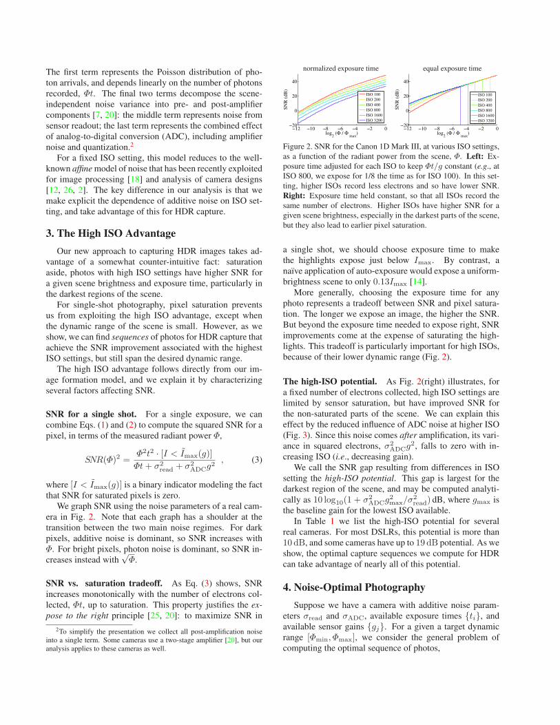
Figure 3. Additive noise (readout and ADC noise) as a function

of ISO for the Canon 1D Mark III [7]. Left: In terms of the raw

pixel value I , additive noise (in DN) increases with ISO. Right:

Relative to the number of electrons recorded, Φt, additive noise

(in electrons) falls with ISO.

camera release pixel high-ISOmodel date pitch (µm) potential (dB)

Nikon D3 2007 8.5 11.1

Canon 1D Mark II 2004 8.2 17.9

Canon 1D Mark III 2007 7.2 15.7

Canon 5D Mark II 2008 6.4 19.7

Canon 350D 2005 6.4 15.3

Nikon D300 2007 5.5 3.1

Canon S70 2004 2.3 2.2

Table 1. High-ISO potential for various digital cameras, highlight-

ing the camera we used in our experiments (noise data from [7]).

This potential is generally higher for cameras with larger pixels,

because their lower gain limits amplifier performance.

• maximizing worst-case SNR, within a given capture

time budget of tmax, or

• minimizing total capture time, for a given minimum

acceptable SNR, SNRmin.

Solving either of these problems requires answering two

questions. First, how do we predict the worst-case SNR

from a given capture sequence? Second, how can we solve

the optimization in a tractable way?

4.1. Merging pixel measurements

To predict the SNR for a given capture sequence, we de-

rive an optimal estimator for the merged result, and show

that its squared SNR has a particularly simple form.

Optimal pixel merging. For a given pixel, we consider a

set of raw measurements Ik, captured with exposure times

ti(k) and sensor gains gj(k), and seek an optimal estimate

for the radiant power Φ. From Eq. (1) it is straightforward

to derive the minimum-variance unbiased estimator:

Φ =

∑

k wk · (Ik − I0)gj(k)/ti(k)∑

k wk(4)

Var(Φ) =1

∑

k wk, (5)

with blending weights defined by

wk =t2i(k) · [Ik < Imax(gj(k))]

g2j(k)Var(nk). (6)

For a fixed ISO setting, this method is equivalent to the

variance-based weighting proposed by [16]. Unlike other

HDR merging methods [8, 22, 6, 10, 3], our weighting

scheme is both well-founded and incorporates a detailed

model of sensor noise. To estimate Var(nk) in practice, we

approximate Φ for observed pixel value Ik using Eq. (1),

and then evaluate Eq. (2) using this estimate.

SNR of the merged estimate. Using the optimal estima-

tor above, we can derive an expression for the squared SNR

of the merged measurement, analogous to Eq. (3):

SNR(Φ)2 =Φ2

Var(Φ)=

∑

i,j

mij ·Φ2t2i · [Iij < Imax(gj)]

Φti + σ2read + σ2

ADCg2j

(7)

where mij is the number of photos captured with expo-

sure time ti and sensor gain gj . This equation shows that

squared SNR for a capture sequence has the particularly

simple property of being linear in the number of photos per

camera setting. This is important because it allows us to

express our optimization in a tractable way.

As shown in Fig. 4, the SNR of a given HDR capture

sequence follows a sawtooth pattern, with the sudden drops

corresponding to saturation points of individual photos.

4.2. Optimization

Worst-case SNR. To evaluate worst-case SNR for a given

capture sequence, we can evaluate the formula in Eq. (7) at

a finite set of keypoints for the radiant power and take the

minimum. In particular, the piecewise montonocity of SNR

means that we need only consider the boundaries of the dy-

namic range, plus intermediate keypoints corresponding to

the saturation points for each photo in the sequence:

K = {Φmin, Φmax} ∪({

(Imax − I0)gj(k)/ti(k) + ε}

∩ [Φmin, Φmax]), (8)

where ε is a small constant (we use 10−8), that lets us eval-

uate SNR numerically just past each saturation point.

Optimal capture sequences. By combining Eqs. (7) and

(8), we obtain a finite number of linear inequalities that let

us fully characterize the optimal capture sequence for each

of our objectives.

Theorem 1 (SNR-Optimal Capture Sequence). For a given

time budget tmax, the capture sequence maximizing worst-

case SNR over the dynamic range [Φmin, Φmax] is the solu-

tion to the mixed integer programming problem:

maximize SNR2worst (9)

subject to∑

i,j mij(ti + tover) ≤ tmax + tover (10)

SNR(Φ)2 ≥ SNR2worst for all Φ ∈ K (11)

mij ≥ 0 and integer , (12)

where SNRworst is the worst-case SNR; mij are the multi-

plicities, counting how many times camera setting (ti, gj)appears in the capture sequence; tover is the overhead time

between shots; and K are the keypoints defined in Eq. (8)

for all available camera settings.

The optimization of total capture time is can be formu-

lated in a very similar way.

Theorem 2 (Time-Optimal Capture Sequence). For a

given minimum SNR, SNRmin, over the dynamic range

[Φmin, Φmax], the capture sequence minimizing total cap-

ture time is the solution to:

minimize∑

i,j mij(ti + tover) (13)

subject to SNR2worst ≥ SNR2

min (14)

and also subject to Eqs. (11)–(12).

While it is not possible to establish a closed-form ex-

pression for the optimal sequence in either case, solving the

integer programs in Theorems 1-2 is straightforward using

readily-available tools [1]. Note that optimal capture se-

quences for a given camera can be precomputed offline, so

fast runtime is not our main concern.

When comparing our optimal capture sequence to a ref-

erence, another fair way to control for camera overhead is

to set tover to zero, but limit the number of photos in the

optimal sequence to be the same as in the reference se-

quence. We can implement this by adding a new constraint,∑

i,j mij = mmax, to the integer program. This formula-

tion has the advantage of equalizing total camera overhead

but avoiding tradeoffs that depend on the absolute bright-

ness of the scene.

We also consider an even more constrained variant of the

optimization, where the exposure times are fixed and only

ISO setting is allowed to vary. This can be implemented

by adding constraints {∑

j mij = mi}, where mi is the

number of photos with exposure time ti in the reference.

5. Results and Discussion

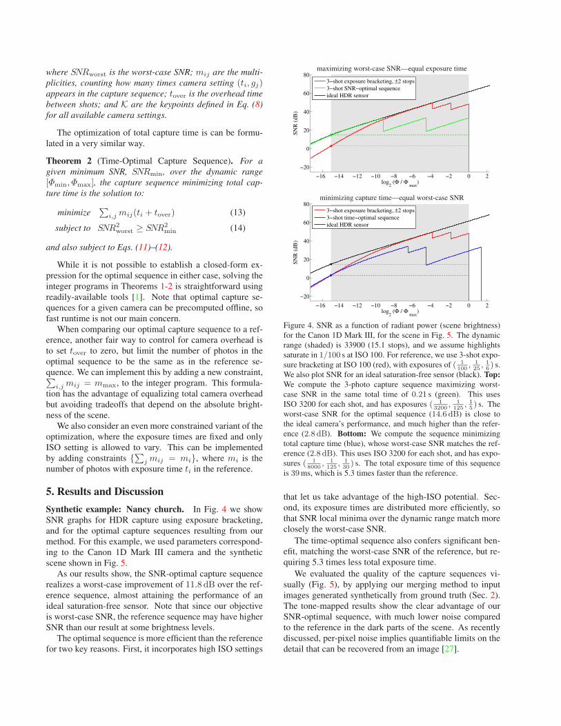
Synthetic example: Nancy church. In Fig. 4 we show

SNR graphs for HDR capture using exposure bracketing,

and for the optimal capture sequences resulting from our

method. For this example, we used parameters correspond-

ing to the Canon 1D Mark III camera and the synthetic

scene shown in Fig. 5.

As our results show, the SNR-optimal capture sequence

realizes a worst-case improvement of 11.8 dB over the ref-

erence sequence, almost attaining the performance of an

ideal saturation-free sensor. Note that since our objective

is worst-case SNR, the reference sequence may have higher

SNR than our result at some brightness levels.

The optimal sequence is more efficient than the reference

for two key reasons. First, it incorporates high ISO settings

maximizing worst-case SNR—equal exposure time

−16 −14 −12 −10 −8 −6 −4 −2 0 2

−20

0

20

40

60

80

log2 (Φ / Φ

max)

SN

R (

dB

)

3−shot exposure bracketing, ±2 stops

3−shot SNR−optimal sequence

ideal HDR sensor

minimizing capture time—equal worst-case SNR

−16 −14 −12 −10 −8 −6 −4 −2 0 2

−20

0

20

40

60

80

log2 (Φ / Φ

max)

SN

R (

dB

)

3−shot exposure bracketing, ±2 stops

3−shot time−optimal sequence

ideal HDR sensor

Figure 4. SNR as a function of radiant power (scene brightness)

for the Canon 1D Mark III, for the scene in Fig. 5. The dynamic

range (shaded) is 33900 (15.1 stops), and we assume highlights

saturate in 1/100 s at ISO 100. For reference, we use 3-shot expo-

sure bracketing at ISO 100 (red), with exposures of ( 1100

, 125, 16) s.

We also plot SNR for an ideal saturation-free sensor (black). Top:

We compute the 3-photo capture sequence maximizing worst-

case SNR in the same total time of 0.21 s (green). This uses

ISO 3200 for each shot, and has exposures ( 13200

, 1125

, 15) s. The

worst-case SNR for the optimal sequence (14.6 dB) is close to

the ideal camera’s performance, and much higher than the refer-

ence (2.8 dB). Bottom: We compute the sequence minimizing

total capture time (blue), whose worst-case SNR matches the ref-

erence (2.8 dB). This uses ISO 3200 for each shot, and has expo-

sures ( 18000

, 1125

, 130) s. The total exposure time of this sequence

is 39ms, which is 5.3 times faster than the reference.

that let us take advantage of the high-ISO potential. Sec-

ond, its exposure times are distributed more efficiently, so

that SNR local minima over the dynamic range match more

closely the worst-case SNR.

The time-optimal sequence also confers significant ben-

efit, matching the worst-case SNR of the reference, but re-

quiring 5.3 times less total exposure time.

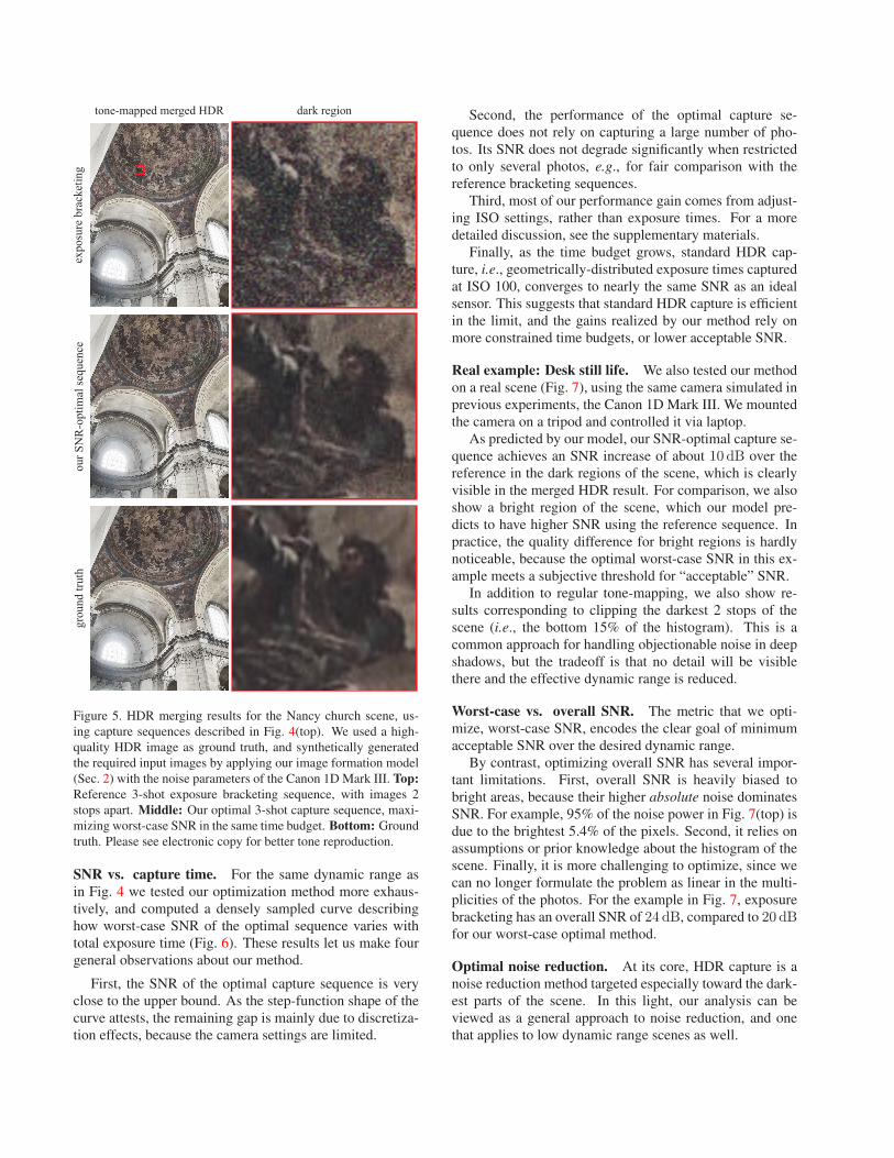
We evaluated the quality of the capture sequences vi-

sually (Fig. 5), by applying our merging method to input

images generated synthetically from ground truth (Sec. 2).

The tone-mapped results show the clear advantage of our

SNR-optimal sequence, with much lower noise compared

to the reference in the dark parts of the scene. As recently

discussed, per-pixel noise implies quantifiable limits on the

detail that can be recovered from an image [27].

gro

un

d t

ruth

ou

r S

NR

-op

tim

al s

equ

ence

exp

osu

re b

rack

etin

g

tone-mapped merged HDR dark region

Figure 5. HDR merging results for the Nancy church scene, us-

ing capture sequences described in Fig. 4(top). We used a high-

quality HDR image as ground truth, and synthetically generated

the required input images by applying our image formation model

(Sec. 2) with the noise parameters of the Canon 1D Mark III. Top:

Reference 3-shot exposure bracketing sequence, with images 2

stops apart. Middle: Our optimal 3-shot capture sequence, maxi-

mizing worst-case SNR in the same time budget. Bottom: Ground

truth. Please see electronic copy for better tone reproduction.

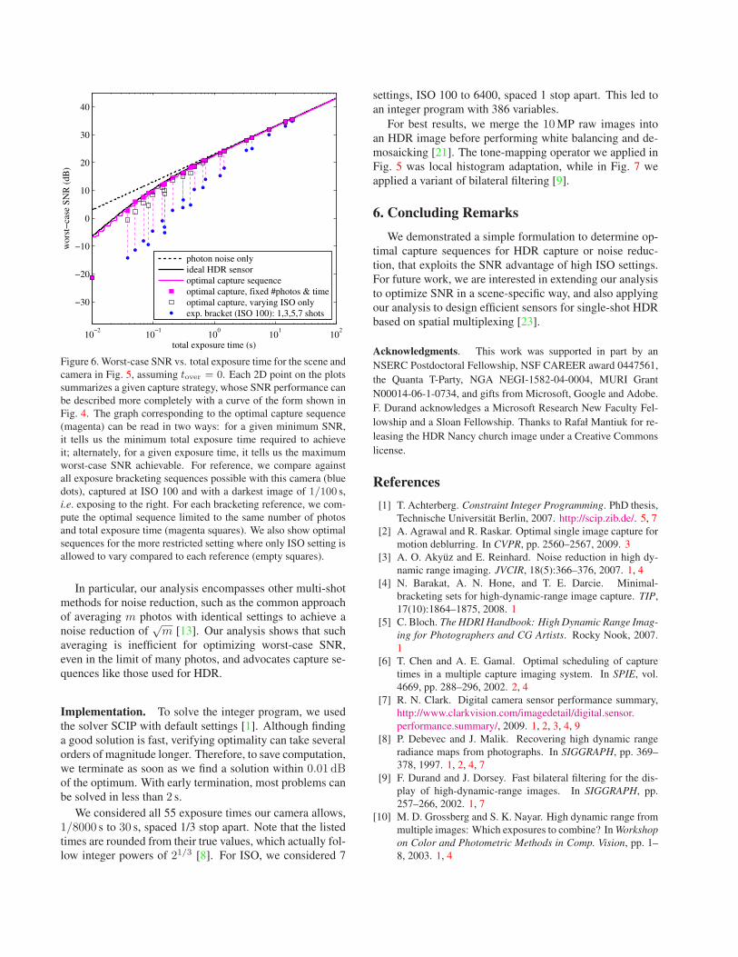
SNR vs. capture time. For the same dynamic range as

in Fig. 4 we tested our optimization method more exhaus-

tively, and computed a densely sampled curve describing

how worst-case SNR of the optimal sequence varies with

total exposure time (Fig. 6). These results let us make four

general observations about our method.

First, the SNR of the optimal capture sequence is very

close to the upper bound. As the step-function shape of the

curve attests, the remaining gap is mainly due to discretiza-

tion effects, because the camera settings are limited.

Second, the performance of the optimal capture se-

quence does not rely on capturing a large number of pho-

tos. Its SNR does not degrade significantly when restricted

to only several photos, e.g., for fair comparison with the

reference bracketing sequences.

Third, most of our performance gain comes from adjust-

ing ISO settings, rather than exposure times. For a more

detailed discussion, see the supplementary materials.

Finally, as the time budget grows, standard HDR cap-

ture, i.e., geometrically-distributed exposure times captured

at ISO 100, converges to nearly the same SNR as an ideal

sensor. This suggests that standard HDR capture is efficient

in the limit, and the gains realized by our method rely on

more constrained time budgets, or lower acceptable SNR.

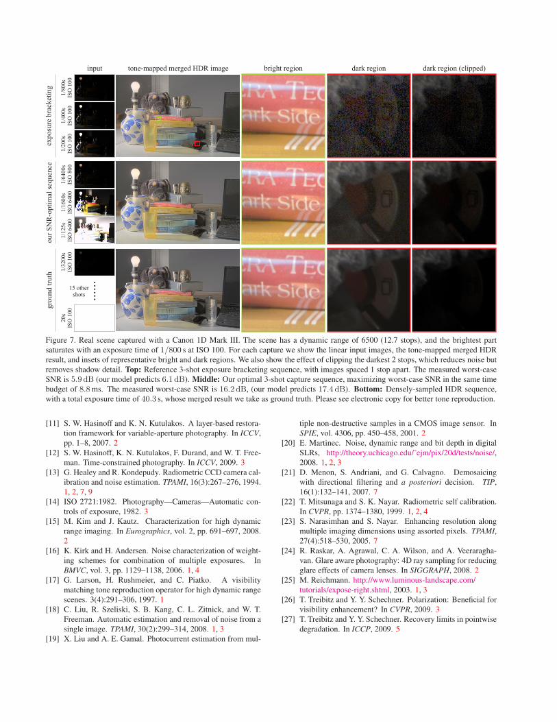
Real example: Desk still life. We also tested our method

on a real scene (Fig. 7), using the same camera simulated in

previous experiments, the Canon 1D Mark III. We mounted

the camera on a tripod and controlled it via laptop.

As predicted by our model, our SNR-optimal capture se-

quence achieves an SNR increase of about 10 dB over the

reference in the dark regions of the scene, which is clearly

visible in the merged HDR result. For comparison, we also

show a bright region of the scene, which our model pre-

dicts to have higher SNR using the reference sequence. In

practice, the quality difference for bright regions is hardly

noticeable, because the optimal worst-case SNR in this ex-

ample meets a subjective threshold for “acceptable” SNR.

In addition to regular tone-mapping, we also show re-

sults corresponding to clipping the darkest 2 stops of the

scene (i.e., the bottom 15% of the histogram). This is a

common approach for handling objectionable noise in deep

shadows, but the tradeoff is that no detail will be visible

there and the effective dynamic range is reduced.

Worst-case vs. overall SNR. The metric that we opti-

mize, worst-case SNR, encodes the clear goal of minimum

acceptable SNR over the desired dynamic range.

By contrast, optimizing overall SNR has several impor-

tant limitations. First, overall SNR is heavily biased to

bright areas, because their higher absolute noise dominates

SNR. For example, 95% of the noise power in Fig. 7(top) is

due to the brightest 5.4% of the pixels. Second, it relies on

assumptions or prior knowledge about the histogram of the

scene. Finally, it is more challenging to optimize, since we

can no longer formulate the problem as linear in the multi-

plicities of the photos. For the example in Fig. 7, exposure

bracketing has an overall SNR of 24 dB, compared to 20 dBfor our worst-case optimal method.

Optimal noise reduction. At its core, HDR capture is a

noise reduction method targeted especially toward the dark-

est parts of the scene. In this light, our analysis can be

viewed as a general approach to noise reduction, and one

that applies to low dynamic range scenes as well.

10−2

10−1

100

101

102

−30

−20

−10

0

10

20

30

40

total exposure time (s)

wo

rst−

case

SN

R (

dB

)

photon noise only

ideal HDR sensor

optimal capture sequence

optimal capture, fixed #photos & time

optimal capture, varying ISO only

exp. bracket (ISO 100): 1,3,5,7 shots

Figure 6. Worst-case SNR vs. total exposure time for the scene and

camera in Fig. 5, assuming tover = 0. Each 2D point on the plots

summarizes a given capture strategy, whose SNR performance can

be described more completely with a curve of the form shown in

Fig. 4. The graph corresponding to the optimal capture sequence

(magenta) can be read in two ways: for a given minimum SNR,

it tells us the minimum total exposure time required to achieve

it; alternately, for a given exposure time, it tells us the maximum

worst-case SNR achievable. For reference, we compare against

all exposure bracketing sequences possible with this camera (blue

dots), captured at ISO 100 and with a darkest image of 1/100 s,

i.e. exposing to the right. For each bracketing reference, we com-

pute the optimal sequence limited to the same number of photos

and total exposure time (magenta squares). We also show optimal

sequences for the more restricted setting where only ISO setting is

allowed to vary compared to each reference (empty squares).

In particular, our analysis encompasses other multi-shot

methods for noise reduction, such as the common approach

of averaging m photos with identical settings to achieve a

noise reduction of√m [13]. Our analysis shows that such

averaging is inefficient for optimizing worst-case SNR,

even in the limit of many photos, and advocates capture se-

quences like those used for HDR.

Implementation. To solve the integer program, we used

the solver SCIP with default settings [1]. Although finding

a good solution is fast, verifying optimality can take several

orders of magnitude longer. Therefore, to save computation,

we terminate as soon as we find a solution within 0.01 dBof the optimum. With early termination, most problems can

be solved in less than 2 s.

We considered all 55 exposure times our camera allows,

1/8000 s to 30 s, spaced 1/3 stop apart. Note that the listed

times are rounded from their true values, which actually fol-

low integer powers of 21/3 [8]. For ISO, we considered 7

settings, ISO 100 to 6400, spaced 1 stop apart. This led to

an integer program with 386 variables.

For best results, we merge the 10MP raw images into

an HDR image before performing white balancing and de-

mosaicking [21]. The tone-mapping operator we applied in

Fig. 5 was local histogram adaptation, while in Fig. 7 we

applied a variant of bilateral filtering [9].

6. Concluding Remarks

We demonstrated a simple formulation to determine op-

timal capture sequences for HDR capture or noise reduc-

tion, that exploits the SNR advantage of high ISO settings.

For future work, we are interested in extending our analysis

to optimize SNR in a scene-specific way, and also applying

our analysis to design efficient sensors for single-shot HDR

based on spatial multiplexing [23].

Acknowledgments. This work was supported in part by an

NSERC Postdoctoral Fellowship, NSF CAREER award 0447561,

the Quanta T-Party, NGA NEGI-1582-04-0004, MURI Grant

N00014-06-1-0734, and gifts from Microsoft, Google and Adobe.

F. Durand acknowledges a Microsoft Research New Faculty Fel-

lowship and a Sloan Fellowship. Thanks to Rafał Mantiuk for re-

leasing the HDR Nancy church image under a Creative Commons

license.

References

[1] T. Achterberg. Constraint Integer Programming. PhD thesis,

Technische Universitat Berlin, 2007. http://scip.zib.de/. 5, 7

[2] A. Agrawal and R. Raskar. Optimal single image capture for

motion deblurring. In CVPR, pp. 2560–2567, 2009. 3

[3] A. O. Akyuz and E. Reinhard. Noise reduction in high dy-

namic range imaging. JVCIR, 18(5):366–376, 2007. 1, 4

[4] N. Barakat, A. N. Hone, and T. E. Darcie. Minimal-

bracketing sets for high-dynamic-range image capture. TIP,

17(10):1864–1875, 2008. 1

[5] C. Bloch. The HDRI Handbook: High Dynamic Range Imag-

ing for Photographers and CG Artists. Rocky Nook, 2007.

1

[6] T. Chen and A. E. Gamal. Optimal scheduling of capture

times in a multiple capture imaging system. In SPIE, vol.

4669, pp. 288–296, 2002. 2, 4

[7] R. N. Clark. Digital camera sensor performance summary,

http://www.clarkvision.com/imagedetail/digital.sensor.

performance.summary/, 2009. 1, 2, 3, 4, 9

[8] P. Debevec and J. Malik. Recovering high dynamic range

radiance maps from photographs. In SIGGRAPH, pp. 369–

378, 1997. 1, 2, 4, 7

[9] F. Durand and J. Dorsey. Fast bilateral filtering for the dis-

play of high-dynamic-range images. In SIGGRAPH, pp.

257–266, 2002. 1, 7

[10] M. D. Grossberg and S. K. Nayar. High dynamic range from

multiple images: Which exposures to combine? In Workshop

on Color and Photometric Methods in Comp. Vision, pp. 1–

8, 2003. 1, 4

gro

un

d t

ruth

ou

r S

NR

-op

tim

al s

equ

ence

exp

osu

re b

rack

etin

g

1/2

00

s1

/80

0s

1/4

00

s1

/64

00

s1

/12

5s

1/1

60

0s

ISO

64

00

ISO

80

0IS

O 1

00

ISO

10

0IS

O 1

00

ISO

64

00

input tone-mapped merged HDR image dark regionbright region dark region (clipped)2

0s

1/3

20

0s

ISO

10

0IS

O 1

00

......15 other

shots

Figure 7. Real scene captured with a Canon 1D Mark III. The scene has a dynamic range of 6500 (12.7 stops), and the brightest part

saturates with an exposure time of 1/800 s at ISO 100. For each capture we show the linear input images, the tone-mapped merged HDR

result, and insets of representative bright and dark regions. We also show the effect of clipping the darkest 2 stops, which reduces noise but

removes shadow detail. Top: Reference 3-shot exposure bracketing sequence, with images spaced 1 stop apart. The measured worst-case

SNR is 5.9 dB (our model predicts 6.1 dB). Middle: Our optimal 3-shot capture sequence, maximizing worst-case SNR in the same time

budget of 8.8ms. The measured worst-case SNR is 16.2 dB, (our model predicts 17.4 dB). Bottom: Densely-sampled HDR sequence,

with a total exposure time of 40.3 s, whose merged result we take as ground truth. Please see electronic copy for better tone reproduction.

[11] S. W. Hasinoff and K. N. Kutulakos. A layer-based restora-

tion framework for variable-aperture photography. In ICCV,

pp. 1–8, 2007. 2

[12] S. W. Hasinoff, K. N. Kutulakos, F. Durand, and W. T. Free-

man. Time-constrained photography. In ICCV, 2009. 3

[13] G. Healey and R. Kondepudy. Radiometric CCD camera cal-

ibration and noise estimation. TPAMI, 16(3):267–276, 1994.

1, 2, 7, 9

[14] ISO 2721:1982. Photography—Cameras—Automatic con-

trols of exposure, 1982. 3

[15] M. Kim and J. Kautz. Characterization for high dynamic

range imaging. In Eurographics, vol. 2, pp. 691–697, 2008.

2

[16] K. Kirk and H. Andersen. Noise characterization of weight-

ing schemes for combination of multiple exposures. In

BMVC, vol. 3, pp. 1129–1138, 2006. 1, 4

[17] G. Larson, H. Rushmeier, and C. Piatko. A visibility

matching tone reproduction operator for high dynamic range

scenes. 3(4):291–306, 1997. 1

[18] C. Liu, R. Szeliski, S. B. Kang, C. L. Zitnick, and W. T.

Freeman. Automatic estimation and removal of noise from a

single image. TPAMI, 30(2):299–314, 2008. 1, 3

[19] X. Liu and A. E. Gamal. Photocurrent estimation from mul-

tiple non-destructive samples in a CMOS image sensor. In

SPIE, vol. 4306, pp. 450–458, 2001. 2

[20] E. Martinec. Noise, dynamic range and bit depth in digital

SLRs, http://theory.uchicago.edu/˜ejm/pix/20d/tests/noise/,

2008. 1, 2, 3

[21] D. Menon, S. Andriani, and G. Calvagno. Demosaicing

with directional filtering and a posteriori decision. TIP,

16(1):132–141, 2007. 7

[22] T. Mitsunaga and S. K. Nayar. Radiometric self calibration.

In CVPR, pp. 1374–1380, 1999. 1, 2, 4

[23] S. Narasimhan and S. Nayar. Enhancing resolution along

multiple imaging dimensions using assorted pixels. TPAMI,

27(4):518–530, 2005. 7

[24] R. Raskar, A. Agrawal, C. A. Wilson, and A. Veeraragha-

van. Glare aware photography: 4D ray sampling for reducing

glare effects of camera lenses. In SIGGRAPH, 2008. 2

[25] M. Reichmann. http://www.luminous-landscape.com/

tutorials/expose-right.shtml, 2003. 1, 3

[26] T. Treibitz and Y. Y. Schechner. Polarization: Beneficial for

visibility enhancement? In CVPR, 2009. 3

[27] T. Treibitz and Y. Y. Schechner. Recovery limits in pointwise

degradation. In ICCP, 2009. 5