Embed Size (px)
Citation preview
Journal of Dynamics and Differential Equations, VoL 6, No. 3, 1994
Noise and Stability in Differential Delay Equations
Michael C. Maekey ~ and Irina G. Neehaeva 2
Received May 4, 1993
We study the stability of linear stochastic differential delay equations in the presence of additive or multiplieative white and colored noise. Using a stochastic analog of the second Liapunov method, sumeient conditions for mean square and stochastic stability are derived.
KEY WORDS: Differential delay equations; noise; stochastic stability; mean square stability; Liapunov's second method.
1. INTRODUCTION
Differential delay equations have been used to describe the dynamics of laser systems (Hopf et aL, 1982; Ikeda and Matsumoto, 1987), liquid crys- tals (Zhang et aL, 1988), physiological control systems (Glass and Mackey, 1988; Mackey and Milton, 1989; Milton et al., 1990), dynamical diseases (Glass and Mackey, 1979; Mackey and an der Heiden, 1982; Mackey and Glass, 1977; Maekey and Milton, 1987; Milton and Mackey, 1989), and artificial neural network models (Marcus and Westervelt, 1989, 1990) and to explain the oscillations observed in agricultural commodity prices (B61air and Mackey, 1989; Maekey, 1989). Often, though most certainly not always, these differential delay equation models are of the form
dr(t) = -- 7x ( t ) + F ( x ( t -- ~)) (1.1)
dt
with some initial function for x specified on an interval t ~ [ - r, 0] . In this formulation one can think of a state variable x that is "destroyed" at a con-
t Departments of Physiology, Physics, and Mathematics and Center for Nonlinear Dynamics, McGill University, Montreal, Canada. Faculty of Cybernetics, Kicv University, Ukraine.
395
1040-7294/94B)700-0395507.00/0 �9 1994 Pleura Pub~hing Corporation
396 Mackey Ind Nechaeva
stant rate ~ and produced at a rate F that depends on the value of the state variable x a time z in the past. If the function F is monotone increasing, it corresponds to a positive feedback situation, while if it is monotone decreasing we say that it mimics negative feedback. There is a further inter- mediate situation ("mixed" feedback) in which F is monotone increasing over some portion of its domain and decreasing over the remainder (an der Heiden and Mackey, 1982).
To be concrete, consider (1.1) with a specific analytic form for the feedback function F, namely,
dx(t) x " ( t - z ) dt = - ? x ( t ) + ~ 1 + xn( t -~) (1.2)
When O---re<n, Eq. (1.2) would correspond to a situation with negative delayed feedback; with 0 < m < n we have mixed feedback; and when 0 < m--n we have positive feedback. Little is known about the analytic solution properties in these three cases, though a great deal is known based on numerical computations.
In addition to their obvious importance in applications, differential delay equations have also become the focus of intense study in the applied mathematics literature since their numerical solutions may exhibit behaviors ranging from globally stable steady states through stable limit cycle behavior and, finally, culminating in "chaos" as single parameters are varied. Further, it is now well-known that there may be an eventual multi- stability in the limiting solution behavior as the initial function is varied (Crabbet al., 1993; Lesson et al., 1993; Rey and Mackey, 1992, 1993).
The real world is never as simple as implied by Eq. (1.1) or (1.2), for it is usually the ease that processes are perturbed by noise in one sense or another. Thus, when a measurement is made and irregular behavior is observed, it is not necessarily clear if the result is a signature of chaos or an indication of the effects of externally imposed noise (Longtin and Milton, 1988).
Noise could enter the system (1.1) in one of two generic ways. In the first, we might have the situation in which the dynamics are continuously and additively perturbed by some noise source so the true dynamics are no longer described by (1.1) but rather by
ax(t) dt = - ?x(t) + F ( x ( t - ~)) + a~(t) (1.3)
where ~(t) is some "random" process yet to be specified and defined. This situation is commonly called additive noise for obvious reasons. In the
Noise and Stability in Differential Delay Equations 397
second, we might conceive of a situation in which there is a fluctuation on one of the parameters of (1.1) so the actual dynamics are described by
dx(t) art = -]~x(t)+ F(x(t-x))+G(x(t),x(t-T))~(t) (1.4)
This case is often called multiplicative or parametric noise. Though ultimately we would like to understand the global stability
properties of (1.3) and (1.4) in their full nonlinear form, given the fact that we do not, at the present time, understand the global properties of (1.1) in the absence of noise, this seems an unrealistic goal. What is not unrealistic, however, is to understand the local stability properties of Eqs. (1.3) and (1.4) when they are linearized in the neighborhoods of their steady state(s). That is the goal of this paper. Specifically, we study the stability behavior of the solution of the linear differential delay equation
dx( t ) = ax( t ) + bx( t - ~) + #(x(t)) ~(t) (1.5)
dt
under the influence of perturbations by external whise noise (either additive or multiplicative) or additive colored noise fluctuations. Equation (1.5) is to be Viewed as the linearized version of a nonlinear stochastic differential delay equation in the neighborhood of one of the steady states.
In Section 2, we first present some general mathematical preliminaries that define basic concepts of solutions of stochastic differential delay equa- tions like (1.3) and (1.4) and their stability in a probabilistic sense. In that section we also offer a brief commentary about the techniques we use to prove sufficient conditions for two types of stochastic stability. Section 3 considers the stability properties of a linearized system under the influence Of additive and multiplicative white noise. Section 4 continues our investigation by first examining the role of additive colored noise on the stability of ordinary differential equations, then extending these considera- tions to the effects of additive colored noise on differential delay equations. The paper concludes with a brief discussion in Section 5 in which we con- trast the approach used here (examining the stability of trajectories) with one in which the stability of ensembles is explored through an examination of the evolution of densities via the Fokker-Planck equation.
2. MATHEMATICAL PRELIMINARIES
We denote by ~(t) a stationary Gaussian white noise process with E{~(t)} = 0 and covariance function E{~(t)~(s)} = 6 ( t - s ) , where 6 is the Dirac delta function, and E denotes the mathematical expectation. Colored
398 Maekey and Nechaeva
noise processes will be denoted by r/(t) and described in Section 4. Using the theory of stochastic differential equations we will understand that for- maUy white noise ~(t) is the derivative of the Wiener process w(t) (Arnold, 1974).
Our central interest is the stability of the trivial (x -- 0) solution of the stochastic differential delay equation
dx(t) = f ( t , x,) dt + g(t, x,) dw(t), t >1 0 (2.1)
where x, = x( t + 0), - z <~ 0 <<. O, x( t ) E ~1. The initial condition for (2.1) is
x(O)--#(o), -T~o<<.o (2.2)
where # is an arbitrary continuous deterministic function. In (2.1), w( t )e~P is a standard Wiener process defined on the probability space (/2,/7, P). The Wiener process w(t) has independent stationary Gaussian increments with w(O) = O, E{w(t) - w(s)} = 0, and E{w(t) w(s)} = rain(t, s). The sample trajectories of w(t) are continuous, are nowhere differentiable, and have infinite variation on any finite time interval. The upper limit of Wiener process samples approaches + oo with probability 1 for t ~ oo, while the lower limit is -oo .
A stochastic process x(t) is called a solution of the stochastic differen- tial equation (2.1) when it satisfies, with probability 1, the integral equation
x(t) = x(O) + f ( s , x,) ds + g(s, xs) dw(s)
where the second integral is Itr's stochastic integral (Gihman and Skorohod, 1972; Hasminskii, 1968).
We introduce the following definitions of stability for stochastic differential delay equations (Kolmanovskii and Nosov, 1986).
Def'mition 2.1. The trivial solution of (2.1) is called mean square stable if, for any e > 0, there exists 6(8) > 0 such that for any initial function ~b(0) the inequality
sup 1~(0)12 < ~(8) - ~ ; 0 ~ 0
implies E{Ix(t, ~b)l 2 } < e for t >10 and exponentially mean square stable if, for any positive constants cl and c2,
E{lx(t,q~)12}<~cl sup [q~(O)12exp(-c2t), t>~O --T~8~O
Noise and Stability in Differential Delay Equations 399
Definition 2.2. The trivial solution of Eq. (2.1) is stochastically stable if, for any e t > 0 and e2>0, there exists a 6 > 0 such that for t > 0 the solution x(t, (~) satisfies the inequality
Prob{sup Ix(t, ~)1 ~ s, } ~ 1 - ~2 ~ r sup I~(0)1 ~ 6 t~O - - ~ 0 ~ 0
It follows from the Chebyshev inequality that mean square stability implies stochastic stability (Arnold, 1974).
To prove sufficient stability for equations like (2.1) with delays we use a stochastic analog of Liapunov's second method. This well-known method, developed by Liapunov (1967) for ordinary differential systems, is based on the following idea. A positive definite function v(x) or v(t, x) is selected which plays the role of a generalized distance from the origin (x = 0) to a point x. If along trajectories of the equation this function is noninereasing (dv/dt <~ 0), then the trivial solution x = 0 is stable.
This method was generalized to stochastic differential equations without delays by Hasminskii (1968), Kushner (1967), and Gihman and Skorohod (1972). A Liapunov function v(t, x) for a stochastic differential equation has to be positive definite everywhere on [0, oo)xR ~ and be twice continuously differentiable with respect to x and once continuously differentiable with respect to t. Retarded stochastic differential equations were considered by El'sgol'ts and Norkin (1973), Kolmanovskii and Nosov (1986), and Tsar'kov (1989), where the method of Liapunov-Krasovskii functionals was applied to study stability. Mohammed (1984) has also considered stochastic differential delay equations.
For stochastic differential delay equations it is possible to develop Liapunov's second method in terms of stochastic Liapunov functions jointly with an approach initially proposed by Razumikhin (1956, 1960) for deterministic differential delay equations and clarified by Hale (1977). Namely, if a solution of a differential delay equation begins in a ball and is to leave this ball at some time t, then Ix(t+O)l <Ix(t)[ for all 0r I ' -z , 01. This method was also applied by Nechaeva and Khusainov (1990, 1992a-e) to derive mean square stability conditions for matrix stochastic differential delay equations.
Using this idea we will prove stability conditions for stochastic delay differential equations by contradiction. We will consider the solution of the appropriate equation with a deterministic initial function (2.2) satisfying
sup Ix(0)l <61 (2.3) - - ~ 0 ~ 0
and assume that the solution is not stable. This, in turn, means that there must exist some moment of time t = T> z which is a first exit time of the
865/6/3-4
400 Mackey and Nechaeva
solution from the stability domain with radius p i> 61 about the origin. From this it follows that, except for a subset of probability zero, trajec- tories satisfy
Ix(T-~)1 < Ix(Z)l =p (2.4)
SO
E{Ix(T- x)l 2 } <E{Ix(Y)l'} =p2 (2.5)
when [x(0)12 .< 62. Calculating the stochastic differential of a Liapunov function v(x(T)), we then show that under some conditions the assumption that at t = T the solution leaves the stability domain leads to a contra- diction. In this way sufficient stability conditions are derived.
3. WHITE NOISE
3.1. Additive White Noise
Consider the scalar linear stochastic differential delay equation with additive white noise term
dx(t)= 1'ax(t)+bx(t-z)] dt+adw(t), t>~O (3.1)
where z > 0 is a constant delay, with initial function satisfying (2.3). Using the stochastic analog of Liapunov's second method and choosing a Liapunov function of the form v(x)= Ixl 2 (or alternately v(x)= Ixl'), we derive a sufficient condition for mean square (stochastic) stability of the solutions of (3.1) which is independent of (depends on) the magnitude of z.
Theorem 3.1. I f
o 2 1 a < - I b l 2 Ix(O)l 2 (3.2)
then the solution x(t) of (3.1) is mean square stable, while for
a < - [bl (3.3)
the solution x(t) of (3.1) is stochastically stable.
Proof. Consider the solution x(t) of (3.1) with initial function given by (2.3). To prove condition (3.2) we pick a Liapunov function v(x)= Ixl 2. By It6 differential rule the stochastic differential of v(x(t)) is
dv(x(t)) = I'2 Ix(t)l (ax(t) + bx(t - z)) + o 2] dt + 2 Ix(t)l o dw(t)
Noise and Stability in Differential Delay Equatiom 401
Integrating this relation from zero to t, taking the mathematical expecta- tion of both parts, using the properties of the stochastic integral, and then differentiating with respect to t, we obtain
dE{v(x(t))} <e{2a Ix(t)12 + 2b Ix(t)l x ( t - T) + 0. 2 }
<~E{2a Ix(t)12+2 Ibl Ix(t)l Ix( / -z ) l +0.2} (3.4)
Now assume that x(t) is not mean square stable, which implies that there is some time t = T such that (2.5) holds. From (3.4) and (2.5) we then obtain for t ffi T
d E{v(x(t))} < 2 ( a + Ibl) E{lx(t)l 2} (3.5) +0.2
Solving the differential inequality (3.5) gives
[ 0.2 1 0.2 E{v(x(t))} < E{v(x(O))}+2(a~lbl) e2(a+lbl)t--2(a+lbl) (3.6)
Note that if a + Ibl < 0 holds, then e 2(a+ taD,< 1. Furthermore, assume that
0.2 E{v(x(O))} + 2(a + Ibl) > 0 (3.7)
Then (3.6) and (3.7) together imply that
e{ v(x( t) ) } < e{ v(x(O ) ) } (3.8)
and since v(x) = Ix[ 2, (3.8) becomes
E{ Ix(t)l 2} < Ix(0)l 2
Thus we conclude that
E{ Ix(T)l 2 } < Ix(0)12 < ~ (3.9)
which is clearly in contradiction with (2.5). Thus, with condition (3.7) and a + [b] <0, the assumption that there exists a first exit time T from the stability domain is not valid. Consequently, we have proved mean square stability of x(t) in the sense of Definition 2.1 with t f f i t f f i~ 2. Rewriting (3.7) gives the final form (3.2), which completes the proof of the first statement of the theorem.
402 Mackey and Nechaeva
To prove the stochastic stability condition (3.3) we use a Liapunov function v(x)= Ixl; with r > 0. This leads to the expression
1 Ix(t)l,_2} dt E{v(x(t)) }= E [r Ix(t)[ " - I tax(t)+
< E { r v ( x ) . ~ [ ( a + l b l ) l x ( t ) 1 2 + l a 2 ( r - l Q } (3.10,
for t = T given by (2.4). If we choose 0 < r < 1 and a + Ibl < 0, then from the Chebyshev inequality, stochastic stability for the solution of (3.1) for an arbitrary delay z > 0 follows from (3.10). []
Using the same type of argument when (3.2) or (3.3) do not hold, we can obtain sufficient stability conditions involving the magnitude of T.
Theorem 3.2. I f (3.2) does not hold, then the solution x(t) o f (3.1) is mean square stable for
I a+b+~ r < ~ ' : ~ - ( l a l+ lb l ) Ibl I
(3.11)
when
r 2
a + b < - 2 I[)l'x'0"i (3.12)
I f (3.3) is not valid, then the solution x(t) of (3.1) is stochastically stable for
a + b z<z~w~= (lal+lbl) Ibl (3.13)
with
a + b < 0 (3.14)
Proof. We rewrite (3.1) as
dx(t) = (ax(t) + bx(t) - [bx(t) - bx( t - z)]) dt + e dw(t) (3.15)
Pick a Liapunov function v(x)=[xl 2, and again assume that x(t) with initial function (2.3) is not mean square stable so (2.5) is valid. The stochastic differential of v(x(t)), where x(t) is a solution of (3.15), is then
Noise and Stability in Differential Delay Equations 403
d -dr E{v(x(t)) } = E{2 Ix(t)l [x(t)(a + b) - b[x(t) - x ( t - z)] ] + a 2 }
{ <~E 2 (a+b) tx ( t )12 -2bx ( t ) [ax(s)+bx(s-~)'] ds
< 1"2(a + b ) + 2 Ibl (lal + Ibl)x] E{lx(t)l 2} +a 2
for t = T. Let
2 ( a + b ) + 2 Ibl (lal + Ibl)~ <0, (3.16)
set - k = 2(a + b) + 2 [hi ([a[ + Ibl )z < 0, and solve the inequality
d E{v(x(t))} < -kE{v(x(t))} + a 2
to obtain
E{v(x(t))} <IE{v(x(O))}-~---k l e-k' +a--= ~
Consequently, if
then
E{v(x(O))} - - ~ > 0 (3.17)
E{lx(t)l 2 } < ix(0)l~ < ~2 (3.18)
for t--7". The contradiction between (3.18) and (2.5) leads to the conclu- sion that (3.16) and (3.17) are sufficient for the mean square stability of the solution x(t) of (3.1). Condition (3.11) follows from (3.17). For z positive (3.12) must be satisfied. Thus the proof of the first statement of the theorem is complete.
To prove the stochastic stability conditions (3.13), (3.14), we take a Liapunov function v(x)= Ix[', r > 0 , and assume, as before, that t - T > r is the first exit time of x(t) from the stability domain so (2.4) and (2.5) are valid. Then we obtain, for t-- T,
404 Mackey and Nechaev,=
ddt E{ v(x(t) ) } = E {r Ix(t)l '-I (ax(t) + bx(t) - [bx(t) - bx(t - z)])
1 ix(t)l,_2} + ~ oZr(r- 1)
<~E {rlx(t)l'-' ( (a+b)x(t)-b ft_ [ax(s)+bx(s-x)])
1" 2 ix(t)l,-2} +~o r(r- 1)
<E{E(a+b)+ Ibl (lal + Ibt)x'l r Ix(t)l"
1 ix(t)l,_Z} + ~ o2r(r- 1)
The last expression can be rewritten as
d E{v(x(t))} <E {(a+b+ lbl (lal + lbl)~ + l o 2 ( r - 1 ) ' ~ ) r v ( x ( t ) ) }
(3.19) where t = T. If
a+b+ Ibl ( a + b ) z < 0 (3.20)
and we choose 0 < r < I, then the stochastic stability of x(t) follows from (3.19) by using Chebysbev's inequality. Inequality (3.20) implies (3.13) and (3.14). [ ]
Remark 1. The comparison of these results with the stability conditions for stochastic ordinary differential equations and deterministic differential delay equations is instructive.
Setting o = 0 Eq. (3.1) reduces to the deterministic delay differential equation
dx ffi ax(t) + bx(t- ~) (3.21)
for which it is known (Ersgorts, 1966; Glass and Mackey, 1988; Hale, 1977) that its trivial solution is stable if and only if either a < - Ibl, or
cos-'(-a/b) ~<~Ho~------ ~ , a + b < 0
Noise and Stability in Differential Delay Equations 405
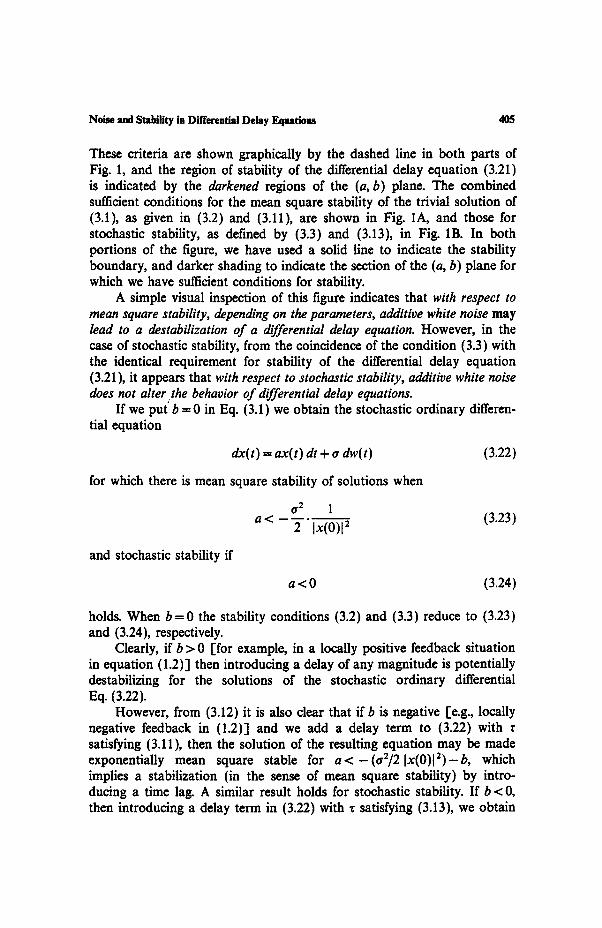
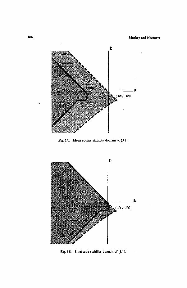
These criteria are shown graphically by the dashed line in both parts of Fig. 1, and the region of stability of the differential delay equation (3.21) is indicated by the darkened regions of the (a, b) plane. The combined sufficient conditions for the mean square stability of the trivial solution of (3.1), as given in (3.2) and (3.11), are shown in Fig. IA, and those for stochastic stability, as defined by (3.3) and (3.13), in Fig. lB. In both portions of the figure, we have used a solid line to indicate the stability boundary, and darker shading to indicate the section of the (a, b) plane for which we have sufficient conditions for stability.
A simple visual inspection of this figure indicates that with respect to mean square stability, depending on the parameters, additive white noise m a y
lead to a destabilization o f a differential delay equation. However, in the case of stochastic stability, from the coincidence of the condition (3.3) with the identical requirement for stability of the differential delay equation (3.21), it appears that with respect to stochastic stability, additive white noise does not alter the behavior of differential delay equations.
If we put:b = 0 in Eq. (3.1) we obtain the stochastic ordinary differen- tial equation
dx(t) = ax(t) dt + 0- dw(t) (3.22)
for which there is mean square stability of solutions when
0 -2 1
a < -- -~- �9 ix(0)[------ ~ (3.23)
and stochastic stability if
a < 0 (3.24)
holds. When b =0 the stability conditions (3.2) and (3.3) reduce to (3.23) and (3.24), respectively.
Clearly, if b > 0 [for example, in a locally positive feedback situation in equation (1.2)] then introducing a delay of any magnitude is potentially destabilizing for the solutions of the stochastic ordinary differential Eq. (3.22).
However, from (3.12) it is also clear that if b is negative [e.g., locally negative feedback in (1.2)] and we add a delay term to (3.22) with satisfying (3.11), then the solution of the resulting equation may be made exponentially mean square stable for a < -(0-2/2 [x(O)[2)-b, which implies a stabilization (in the sense of mean square stability) by intro- ducing a time lag. A similar result holds for stochastic stability. If b < 0, then introducing a delay term in (3.22) with T satisfying (3.13), we obtain
406
b
Mackey and Nechaeva
a
I/'c, -l/~)
Fig. 1A. Mean square stability domain of (3.1).
h
l ~ , - l ~ )
Fig. lB. Stochastic stability domain of (3.1).
Noise and Stability in Differential Delay Equations 407
stochastic stability for a < - b , which corresponds to a stabilization with respect to (3.24). Consequently, although introducing an arbitrarily large delay in the stochastic equation will ultimately destabilize the solution, a delay satisfying the criteria of Theorem 3.2 can play a role of stabilizing factor in a locally negative feedback situation. Introducing a delay into a stochastic equation in a locally positive feedback situation is always poten- tially destabilizing. �9
3.2. Multiplicative (Parametric) White Noise
In this section we consider the stability properties of stochastic differential delay equation
dx(t) = lax(t) + b x ( t - ~)] dt + ax(t) dw(t) (3.25)
with parametric white noise and an initial function given by (2.3). Using the same stochastic Liapunov function method, we will derive sufficient stability conditions for the trivial solution of Eq. (3.25).
Theorem 3.3. I f
a < - Ibl - �89 (3.26)
then the trivial solution of (3.25) is exponentially mean square stable. I f
a < - I b l + �89 2 (3.27)
then it is stochastically stable.
Proof. Choosing a Liapunov function v (x )= [xl 2 and assuming that x = 0 is not mean square stable, i.e., (2.5) holds, we have
d dt E{v(x(t))} < e{2a Ix(t)l 2 + 2 Ibl Ix(t)l Ix(t - x)l + o'2x2(t)}
<E{lx(t)12}(2a+2 Ibl + a 2)
at some time t = T. If 2a + 2 Ibl + tr 2 < 0, then
d/ r{v(x( t ) )} < - c/r{ Ix(t)l ~ }
with c = - (2a + 2 Ibt + a2), t = T. From the last inequality we have
/r{ Ix(Z)l }2 < ix(0)12 e-C,< ~
408 Mackey and Nechaeva
which contradicts (2.5). Consequently when (3.26) holds, there is no time at which x(t) exits from the stability domain, and thus condition (3.26) is sufficient for the exponential mean square stability of the trivial solution of (3.25).
To prove (3.27) we take v(x)= Ixl" with r>0 . Using the same reasoning as before, if there is an exit time from the stability domain we obtain the following estimate:
+ { -~ E{v(x(t))} <E ar Ix(t)lr + r Ibl Ix(t)l r - l Ix( t -*) l
+la2 lx(t)l" r (r -1)}
<E {(a+ lbl +Io2(r -1 ) ) r lx(t)l "}
for t = 7'. If
a+lb l + �89 1 )<0 (3.28)
then by the Chebyshev inequality it follows that the trivial solution of (3.25) is stochastically stable. From (3.28) it follows that
2a 2 Ibl 0 < r < l
o 2 O 2
From the positivity of r we find a < (0"2/2) - [bl, which is condition (3.27). []
Theorem 3.4. If the coefficients of Eq. (3.25) do not satisfy condition (3.26), then when a + b < - (o2/2) the trivial solution is exponentially mean square stable for
, { x < x ~ * - - (lal+lbl)lbl a+b+-~ (3.29)
Alternately, if (3.27) does not hold, then when a+ b < o2/2 the trivial solution is stochastically stable for
, { z<T~w*- (lal+lbl)lb[ a + b - ~ (3.30)
Proof. To prove (3.29) we use Liapunov function v(x)--Ixl 2.
Noise and Stability in Differential Delay Equations 409
Assuming as above that x = 0 with an initial function satisfying (2.3) is not mean square stable, i.e., (2.5) is valid, we find from It6's rule that
d E{v(x(t))} ~2(a + b) Ix(t)l f
< E 2
- 2/, Ix(t)l lax(s) + bx(s -- lr)] as + 0.2
<E{E2(a+b)+2 Ibl (lat + Ibl)x +0"23 Ix(t)l 2}
for t = T. Set
-C=2(a+b)+2 Ibl (lal + lb l )x+a2<0 (3.31)
Then from the inequality
~t E{v(x(r))} < - Ce{v(x(I"))}
where C > 0, it follows that there is a contradiction with the assumption that t = T is an exit time from the stability domain, and exponential mean square stability for the trivial solution of (3.25) follows. Inequality (3.31) implies (3.29). The first part of the proof is complete.
To prove the stochastic stability condition (3.30), consider the stochastic differential of v(x(t)) with the Liapunov function v(x)= Ixl'. Let (2.4) hold for the solution of (3.25) with initial function satisfying (2.3). Using It6's rule we obtain
d E{v(x(t))} = E {r Ix(t)l ' - 1 ((a + b) x ( t ) - b[x( t ) - x ( t - x)])
1 2 2 +~a x (t) r ( r - 1) Ix(t)l ' -2}
= E {r Ix(t)l" (a + b) - r Ix(t)l'- '
• b ~!_, lax(s) + bx(s- ~)] as
1 2 Ix(t)l'} +~a r (r - 1)
410 Mackey and Nechaeva
Using (2.4) gives
~ E{v(x(t))} <r a + b + Ibl (lal + )b l )x+ 0-2(r- 1) E{Ix(t)l'}
for t = T. If
a + b + Ibl (lal + lbl)T < �89 - r ) (3.32)
then we can choose r such that
0 < r < l 2 ( a + b ) + 2 [bl ([a[ + Ib])z
0-2
and satisfy the condition
d -~ E{v(x(t)) } < -- CE{v(x(t)) }, C > 0
for t = T, which implies stochastic asymptotic stability of the trivial solu- tion of (3.25) by using Chebyshev inequality. The condition (3.30) follows from (3.32). []
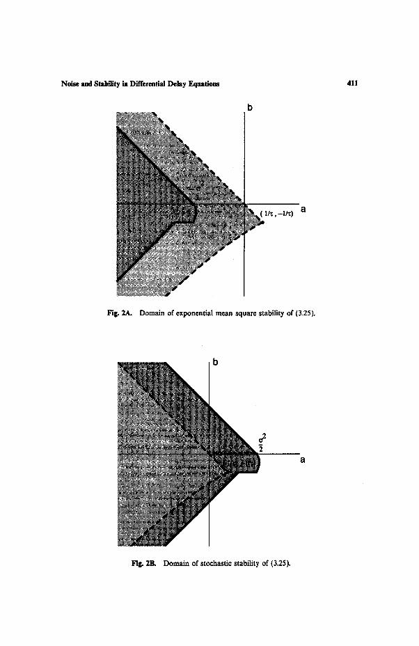
Remark 2. As in Fig. 1, in Fig. 2 we plot the boundary of the stability region for the differential delay equation (3.21) by a dashed line and indicate the stability region of the (a, b) plane by the darkened area.
If we set b = 0, so (3.25) reduces to the ordinary stochastic differential equation with multiplicative white noise)
dx(t) = ax(t) dt + 0-x(t) dw(t) (3.33)
and (3.26) and (3.27) yield well-known conditions for exponential mean square stability (Arnold, 1974)
0-2
2
and stochastic stability (Arnold, 1974; Hasminskii, 1968)
0-2 a < m
2
of the trivial solution of the stochastic ordinary differential equation. In Fig. 2A we have plotted the stability boundary for exponential
Noise and Stability in Differential Delay Equations 411
a l/x, -l/x)
Fig. 2A. Domain of exponential mean square stability of (3.25).
Fig. 2B. Domain of stochastic stability of (3.25).
412 Maekey and Nechaeva
mean square stability [Eqs. (3.26) and (3.29)] as a solid line and indicated the stability domain by darker shading A visual inspection of that figure makes it clear that, with respect to mean square stability, multiplicative white noise may lead to a destabilization of a differential delay equation, and addition of delayed effects may either stabilize or destabilize a stochastic system with multiplicative white noise.
Figure 2B shows the stability domain for stochastic stability, bounded by the conditions (3.27) and (3.30), drawn as solid lines. In this case it is clear that multiplicative white noise always leads to a stabilization of the trivial solution of the differential delay equation (3.21), and the addition of a delay may either stabilize or destabilize a stochastic system with multi- plicative whRe noise.
We can understand this delay-induced stabilization of a stochastic system by choosing b negative and adding in (3.33) a delay term with satisfying (3.29). Then we have exponential mean square stability for a < - ( ~ r 2 / 2 ) - b . Similarly, with b < 0 and ~ given by (3.30), we have stochastic stability for a < (tr2/2) - b. Consequently, with b < 0 it is possible to stabilize a system by introducing a time delay satisfying the conditions of Theorem 3.4. Conclusions similar to these, obtained using the Liapunov-Krasovskii functionals, were found by El'sgol'ts and Norkin (1973) and Kolmanovskii and Nosov (1986). �9
4. ADDITIVE COLORED NOISE
Before considering the effects of additive colored noise in differential delay equations, we first treat the effect in ordinary differential equations since the results we present seen to be new.
4.1. Ordinary Differential Equations with Additive Colored Noise
This section presents sufficient stability conditions for an ordinary differential equation with additive colored noise.
Consider a stochastic process x(t) which satisfies the equation
dx(t) = ax(t) dt + ~(t) dt, t >t 0, x(0) ffi x o (4.1)
where x ( t ) e ~ ' , tl(t) is a colored noise term modeled by the Ornstein- Uhlenbeck process (Arnold, 1974) which satisfies the Langevin equation
~ ( t ) dt - ~rt(t)+o~(t)

Noise and Stability in Differential Delay Equations 413
where ~t>0 and a > 0 are constants, and ~(t) is a scalar white noise process. The corresponding stochastic differential equation
dtl(t) = - Oal(t) dt + tr dw(t), t > 0, r/(0) = r/0 (4.2)
is linear in the narrow sense, is autonomous, and has a unique solution (Arnold, 1974),
rl(t) = tloe-~t + a e -~tt-s) dw(s)
where w(t) is a Wiener process, and the stochastic integral is interpreted in the sense of It6. It is known that the Omstein-Uhlenbeck process is stationary, its correlation function is exponentially decreasing, i.e.,
E{ r/(t ) r/(s) } = e-" I,-,la2/2ct
where tr z is the intensity of white noise process ~(t), and E{r E{~( t )~(s )}=tS( t - s ) as before. The stochastic system (4.1), (4.2) with colored noise is equivalent to the pair of processes (x(t), ~l(t)) given by Eqs. (4.1) and (4.2). Although the first component x(t) considered separately is not a Markov process, the pair (x(t), ri(t)) is Markovian.
Write Eqs. (4.1) and (4.2) in the vector form
(x ( t )~= l'~(x(t)~ d X,r/(/)] ( ; d t + ( : ) d w ( , )
-o t /k t l ( t ) /
Introducing the notation
x(t) y ( t )=( t l ( t ) ) , A = ( 0 -l~t)' c=(0tr) (4.3)
we obtain an equation describing the dynamics of the system under the influence of additive colored noise:
dy(t) = Ay(t) dt + c dw(t), t > 0 (4.4)
We assume the initial conditions to be deterministic, so the equalities
E{ Ily(0)ll } = Ily(0)ll
E{ Ily(0)ll 2 } = Ily(0)ll 2 <
hold, where II-II denotes the Euclidean vector norm. The goal of this section is to obtain sufficient stability conditions for
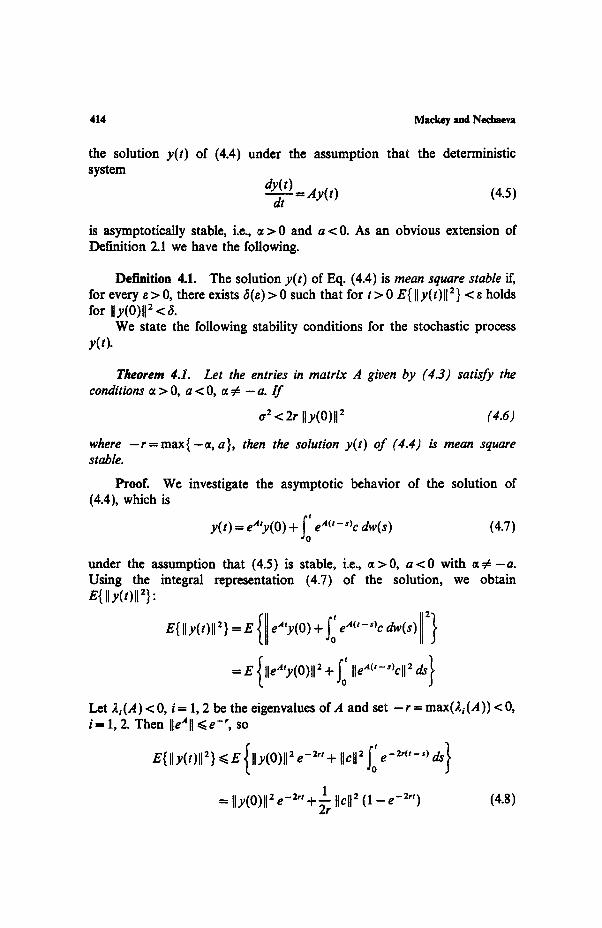
414 Mackey and Nechaeva
the solution y(t) of (4.4) under the assumption that the deterministic system
dY(d: = A y( t ) (4.5)
is asymptotically stable, i.e., 0t > 0 and a < 0. As an obvious extension of Definition 2.1 we have the following.
Def'mition 4.1. The solution y(t) of Eq. (4.4) is mean square stable if, for every 8 > 0, there exists 6(8) > 0 such that for t > 0 E{ I[y(t)H 2 } < 8 holds for Ily(0)ll a < ~.
We state the following stability conditions for the stochastic process y(t).
Theorem 4.1. Let the entries in matrix A given by (4.3) satisfy the conditions ~t > O, a < O, �9 ~ - a. I f
o 2 < 2r Ily(0)ll 2 (4.6)
where - r = m a x { - ~ t , a}, then the solution y(t) o f (4.4) is mean square stable.
Proof. We investigate the asymptotic behavior of the solution of (4.4), which is
y(t) = eAty(O) + Io eA(t- s)c dw(s) (4.7)
under the assumption that (4.5) is stable, i.e., 0~>0, a < 0 with a # - a . Using the integral representation (4.7) of the solution, we obtain E{ Ily(t)ll2}:
E{ ll y(t)ll~} = E { leA'y(O) + fs eA('-*)c dw(s) l ~}
= E { lleA*y(O)ll2 + ~ lleaC'-*'cll2 ds}
Let 21(A) < 0, i = 1, 2 be the eigenvalues of A and set - r = max(2~(A )) < 0, i= 1, 2. Then IleAIt ~ e - ' , so
E{ lly(t)lla} <~E {Jly(0),l 2 e-2" + ,,cJ,~ ~: e - 2 " ( t - s ' ds}
= lly(0)ll ~ e-2"+ 1-- IIc[I 2 (1 - e -2") (4.8) 2r
Noise and Stability in Differential Delay Equations 415
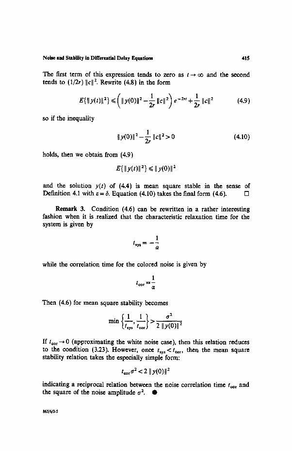
The first term of this expression tends to zero as t ~ oo and the second tends to (1/2r)Ilcll 2. Rewrite (4.8) in the form
1 E{ II y(t)l[ 2 } ~< (lly(0)[I 2 _ 1 i[cl[2 ) e_2. + ~r Ilcjl2 (4.9)
so if the inequality
I II y(0)ll 2 - ~ Ilcll 2 > 0 (4.10)
holds, then we obtain from (4.9)
E{ Ily(t)ll 2 } ~ II y(O)ll 2
and the solution y(t) of (4.4) is mean square stable in the sense of Definition 4.1 with s = & Equation (4.10) takes the final form (4.6). []
Remark 3. Condition (4.6) can be rewritten in a rather interesting fashion when it is realized that the characteristic relaxation time for the system is given by
1 tsy s -~ - - -- a
while the correlation time for the colored noise is given by
1 tOO r ~
Then (4.6) for mean square stability becomes
0-2
min ~ 1 ' t-~} > 2 Ijy(0)ll 2 ( t s y s
If tcor -'} 0 (approximating the white noise case), then this relation reduces to the condition (3.23). However, once t , . < t,o~, then the mean square stability relation takes the especially simple form:
tcorO2 < 2 Ily(0)ll 2
indicating a reciprocal relation between the noise correlation time t~r and the square of the noise amplitude o 2. �9
~ss/q3-s
416 Mackey and Nechaeva
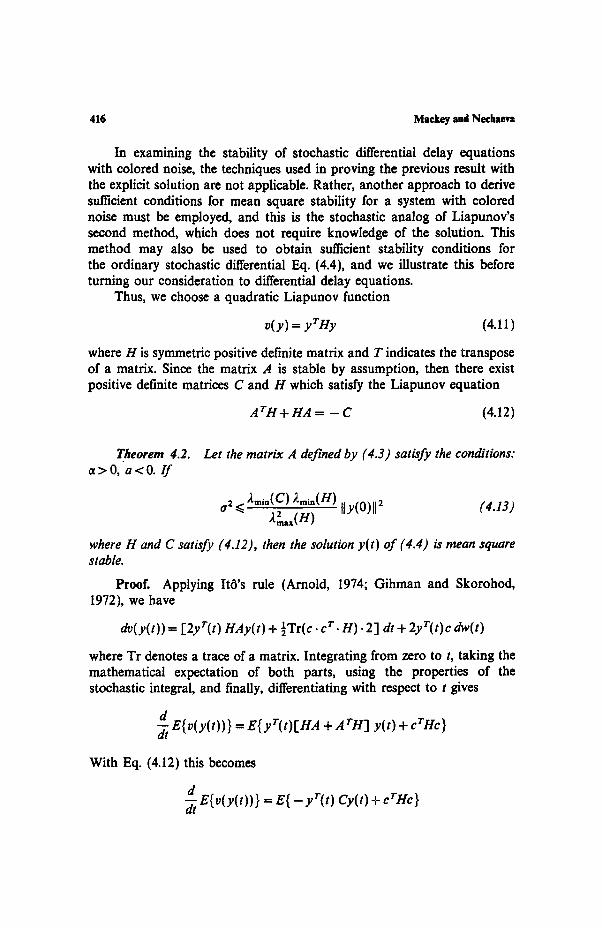
In examining the stability of stochastic differential delay equations with colored noise, the techniques used in proving the previous result with the explicit solution are not applicable. Rather, another approach to derive sufficient conditions for mean square stability for a system with colored noise must be employed, and this is the stochastic analog of Liapunov's second method, which does not require knowledge of the solution. This method may also be used to obtain sufficient stability conditions for the ordinary stochastic differential Eq. (4.4), and we illustrate this before turning our consideration to differential delay equations.
Thus, we choose a quadratic Liapunov function
v(y) = yrHy (4.11)
where H is symmetric positive definite matrix and T indicates the transpose of a matrix. Since the matrix ,4 is stable by assumption, then there exist positive definite matrices C and H which satisfy the Liapunov equation
A r H + H A = - C (4.12)
Theorem 4.2. ~>O, a<O. If
Let the matrix A defined by (4.3) satisfy the conditions:
~2 ~< ~.m~(C) :.~(H) II y(0)ll 2 (4.13)
where H and C satisfy (4.12), then the solution y(t) of (4.4) is mean square stable.
Proof. Applying It6's rule (Arnold, 1974; Gihman and Skorohod, 1972), we have
dv(y(t)) = [2yr(t) HAy(t) + �89 c r. H). 2] dt + 2yr(t)c dw(t)
where Tr denotes a trace of a matrix. Integrating from zero to t, taking the mathematical expectation of both parts, using the properties of the stochastic integral, and finally, differentiating with respect to t gives
d E{v(y(t)) } = E{ yr(t)[ HA + A rH] y(t) + crHc}
With Eq. (4.12) this becomes
d "dt E{v(y(t)) } = E{ - yr(t) Cy(t) + crHc}
Noise and Stability in Differential Delay Equations 417
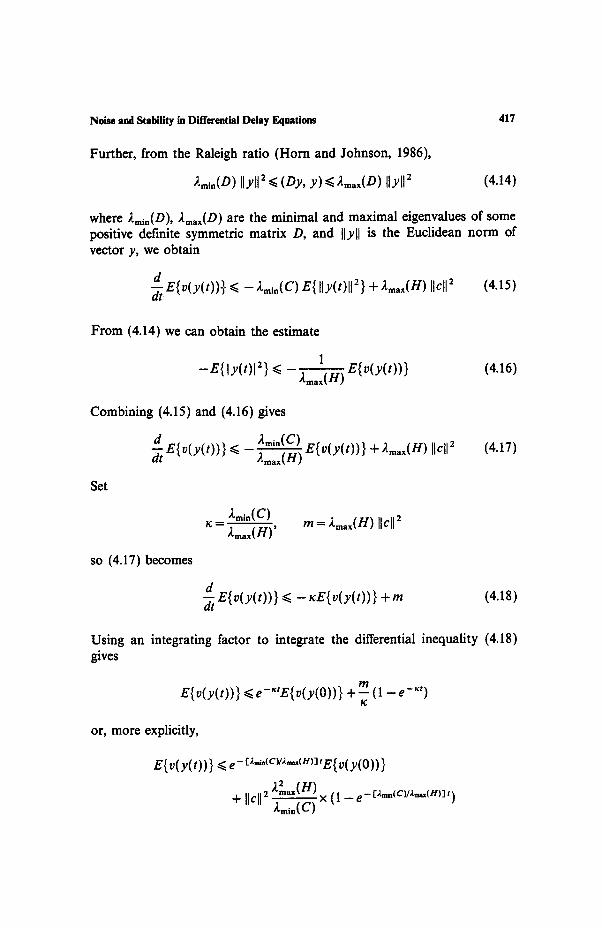
Further, from the Raleigh ratio (Horn and Johnson, 1986),
).rain(D) Ilyll 2 ~< (Dy, y) <~ Amax(D ) 117115 (4.14)
where 2rain(D), ~.max(D) are the minimal and maximal eigenvalues of some positive definite symmetric matrix D, and IlYll is the Euclidean norm of vector y, we obtain
d E{v(y(t)).} <~ - 2=i.(C) E{ II y(t)ll 2 } + 2=~,(H) Ilcll 2 (4.15)
From (4.14) we can obtain the estimate
1 -E{ly(t)l 2} <<. E{v(y(t))} (4.16) 2max(H)
Combining (4.15) and (4.16) gives
d 2min(C) "T E{v(y(t))} <~ E{v(y(t))} + 2max(H)Ilcll 2 2max(H) at
(4.17)
Set
x = - - m = 2 m x ( H ) I l c l l 2 ~m~,(n)'
so (4.17) becomes
d ~ E{v(y(t)) } <~ -xE{v(y(t)) } + m (4.18)
Using an integrating factor to integrate the differential inequality (4.18) ~ves
•t m e _ ~ t ) E{v(y(t))} <.e- E{v(y(O))} +--(1 - Ir
or, more explicitly,
E{v(y(t))} <~ e- [~.r tE{v(y(O)) }
2~,(H) (l_e_[~8(c)/~,~(n)lt) + Ilcll2 ).mi.(C-----'~ x
418
and finally,
t a . , . ~ c ~ . ~ , FE{v(y(o)) } _ ,tL,,(H)l g{v(y(t))} <~ e - - Ilcll~ 2=i.(C) ] L .
+ Ilcll ~mm(C)
If
holds so
z{o(y(0))} - Ilcll 2 ~ > u
lVlackey snd Nechaeva
(4.19)
2~.~(C) E{v(y(0))} (4.20) Ilcll2 < ,~ , , (H)
then it follows from (4.19) that
E{v(y(t))} <~ E{v(y(O))} (4.21)
Because the Liapunov function v(y) is a quadratic form and the matrix H is positive definite, we obtain from (4.21)
2=~(H) < 6 (4.22) E{Ily(t)It2} <~ Ily(0)II2 2.,~,(H) 2,,i.(n)
Therefore it follows from (4.2d23) that the solution y(t) of (4.4) is mean square stable in the sense of Definition 4.1 with ~(e) = (2=i~(H)/Xmax(H))e, if (4.20) holds. Using the estimate
2m~,(H) Ily(0)ll ~ ~< yr(O) Hy(O) = o(y(0))
condition (4.20) takes the final form (4.13). E]
Remark 4. We see that the estimate (4.13) is expressed by the eigen- values of positive definite matrices C and H satisfying Liapunov's equation (4.12). The problem of finding maximal value of the noise amplitude o 2 under which the stability is preserved leads to the optimization problem
Noise and Stability in Differential Delay Equations
where
2rain( - - A r H - H A ) 2rain(H) , ( /- t) -
with L = {H: H = H r > O } , so L is equivalent to
L = { n : > o}
419
An analogous problem has been considered by Bychkov et al. (1992). �9
4.2. Differential Delay Equations with Additive Colored Noise
These Liapunov-type techniques can also be used to obtain sufficient stability conditions for delay differential equations with additive colored noise like
dx(t) = I'ax(t) + bx(t - ~)'1 dt + rl(t ) dt,
drl(t) = - ~rl(t) dt + a dw(t),
x(O)=4(o), -~<~0<~0 (4.23)
~(0)=% (4.24)
where x ( t ) e ~ t, r/(t) is an Ornstein-Uhlenbeck process defined above, z > 0 is a constant delay, $ is continuous deterministic function. We will study stability properties of the solution x( t ) of the differential delay equation (4.23) perturbed by colored noise t/(t) by considering the pair (x(t) , ~l(t)), and denote this two-component process by y(t). Using the same notation as in (4.3) and further defining
we can reduce the system (4.23), (4.24) to
dy(t) = lAy ( t ) + By( t - ~)] dt + c dw(t) (4.25)
By a solution of (4.25), we mean the stochastic process y( t ) defined by the integral equation
y( t ) = y(O) + lAy ( s ) + B y ( s - ~)] ds + c dw(s)
where the last integral is a stochastic It6 integral. To define an initial func-
420 Maekey and Neehaeva
tion y(O)=(~(O), -T<~O<~O for (4.25), we will consider formally that t/(0) = t/o. We assume that y(O) satisfies
sup Ily(0)ll <~ (4.26) - - ~ 0 ~ 0
where li'll denotes Euclidean vector norm. We will prove a mean square stability condition for the solution of (4.25) with initial function (4.26) using the stochastic analog of Liapunov's direct method. The definition of mean square stability for the solution y(t) of (4.25) is analogous to that in Definition 3.1 with norm II-II instead of l.I.
We assume that unperturbed system with z = 0, i.e., the deterministic system without delay,
dy(t) = (A + B) y(t) dt (4.27)
is asymptotically stable, and use a Liapunov function v(y) defined by (4.11) in conjunction with a symmetric positive definite matrix H which satisfies the Liapunov equation
(A + B) r H + H(A + B) = - C (4.28)
Theorem 4.3. Let H and C be positive definite matrices satisfying the Liapunoo equation (4.28), the matrix A + B be stable, and assume the condition
2max(H)~ > 0 (4.29) 2mi,(C)-2 IIHBll 1 -t ~,min(n),]
is satisfied. Then i f
tr 2 ~ < 2m'n(H) [2mi , (C)-2 'IHBII (1 + Ama.(a)'~q 2~ax(H ) 2~in(H)/J Ily(0)[12 (4.30)
the solution y(t) o f (4.25) is mean square stable.
Proof. Assume that y(t) is not mean square stable so T> z is the first exit time of the process y( t ) from the stability domain of radius 8 > t~ about the origin, i.e.,
E{ I I y ( T - ~)ll 2 } < E{ It y(T)ll 2 } = 8 (4.31)
From the stochastic differential of v(y(t)), t = T, and techniques similar to those used in the proof of Theorem 3.1 and Theorem 4.2, we obtain
d E{v(y( t ) )} = g{yr(t)[H(A + B) + (A + B) r H] y(t) -- 2yr(t) HBy( t ) dt
+ 2yr(t) HBy(t -- z) + crHc}
Noise and Stability in Differential Delay Equations 421
From (4.28) and the Raleigh ratio (4.14)
dE{v(y(t))}<<.- [2.i.(C)-2 IIHBII (1-~ 2m'x(H)~l 2=i.(H)J_] E{ Ily(t)l[ 2 }
+ lm~(n) Ilcll = (4.32)
From (4.14) and (4.32) we have the estimate
1 " [2=, .(C)-2 IIHBII (1 +~'max(H)'~] d E{v(y(t))} 2m,~(ff) ~ } J E{v(y(t))}
+ 2m~(H) Ilcll 2
Solving the last inequality we obtain
E{v(x(t))} <.e-kt(E{v(y(O))}-k)+ k (4.33)
where
and
If
holds so
m=2~,,x(H) Ilcll 2
1 I ( Jt'raax(H)'~] k=~.m.=(H) ~m~.(C)-2 IIHBII 1 + ~ / j
m E{o(y(O))}-~>O
E{v(y(O))} [2mi,(C)-2 IIHBII (1 + ~,//2m~(H)Y] Iic112< ~.~(H)
then (4.33) yields
E{v(y(t)) } ~< E{o(y(O))}
Again applying the Raleigh ratio we have
E{ II Y(/)II ~ } ~ II y(0)ll 2 Ama,,(n) 2mi.(H ) < 8
2m.x(H)
(4.34)
422 Msckey and Nedmeva
for t ffi T. Setting 6= (;~maa(H)/lmax(H))8 , we conclude from the contra- diction between the last inequality and (4.31) that there is no exit time from the stability domain under condition (4.34). Thus, (4.34) ensures mean square stability for the solution y(t) of (4.25). Condition (4.34) takes the final form (4.30). From the positivity of Ilcll = the restriction (4.29) follows. [3
Remark 5. An optimization problem analogous to that in Remark 4 can be stated in this case. @
Now we will prove mean square stability conditions that depend on the delay �9 > 0, assuming that the solution of unperturbed ordinary differential system (4.30) is asymptotically stable.
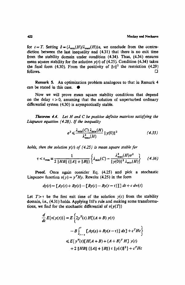
Theorem 4.4. Let H and C be positive definite matrices satisfying the Liapunov equation (4.28). I f the inequality
a2 ~< 2mi.(C) 2mi.(H) 11 y(0)ll 2 (4.35) ~t~,(U)
holds, then the solution y(t) of (4.25) is mean square stable for
{ 1 2, .~.(C) - < Zm,, = 2 IIHB[I ([IAII + [IBII) Ily(0)[I 2 2mi,(H)J
(4.36)
Proof. Once again consider Eq. (4.25) and pick a stochastic Liapunov function v(y)= yrHy. Rewrite (4.25) in the form
dy(t) = lAy(t) + By(t) - [By(t) - B y ( t - z)]] dt + c dw(t)
Let T>~ be the first exit time of the solution y(t) from the stability domain, i.e., (4.31) holds. Applying It6's rule and making some transforma- tions, we find for the stochastic differential of v(y(T))
-~tE{v(y(t))} = E 2yr(t) H[(A + B) y(t)
- ~ - , l i l y ( s ) + B y ( s - ~ ) ] ds ] + c r t t c
~ E{ y~'(t)[H(A + B) + (A + B)~" H] y(t)
+ 2 IIHBII (IIAII + IIBII)~ Ily(t)ll 2 } + c rHc
Noise and Stability in Differential Delay Equations 423
Using (4.28) and (4.14), we can further write
d ~E{v (y ( t ) ) } <. - 12mi,(C)- 2 IIHBII (IIAII + IIBII)CI E Uy(t)ll 2
-t- 2max(n ) Ilcl[ e (4.37)
Let
A~i.~(C) - 2 IIHBII (IIA II + Ilnl})~ > 0
Then from (4.37) we have
~ E{v(y(t)) } ~ -- kE{v(y(t)) } + m
with t = T and
k = 1
l,Ami,(C)-211HBIl(llall+llnll)x] >0, m=A~,~(n) llcll 2
As in the proof of Theorem 4.3 we can show mean square stability for the solution y(t), if
a2<E{v(y(O))}I'kmin(C)-211HBII(IIA]I+]IBI[)~] (4.38)
holds. Inequality (4.36) follows from (4.38), and from the requirement that be positive we obtain (4.35). []
5. CONCLUSIONS
Here we have examined the effects of additive and multiplicative white noise, and additive colored noise, on the stability of the trivial solution of linear differential delay equations by examining the solution trajectory behavior. For stochastic ordinary differential equations, one can examine solution stability and bifurcations by using the Fokker-Planck equation for the evolution of densities (Arnold et al., 1978; Horsthemke and Lcfever, 1984; Knobloch and Wiesenfeld, 1983; Lasota and Mackcy, 1994; Mackey et aL, 1990). However, there is no analog to the Fokker-Planck equation for stochastic equations with a retarded argument l-though some steps have been' made in deriving an evolution equation for densities in differential delay equations unperturbed by noise (see Losson and Mackey, 1992)], and only numerical results are available concerning the influence of colored
424 Maekey and Neehaeva
noise on the density behavior of stochastic differential delay equations (Longtin et al., 1990; Longtin, 1991).
As in other work, the results of this paper highlight the difficulties of studying colored noise effects in comparison to white noise. Using the stochastic analog of Liapunov's second method has allowed us to investigate analytically the effects of additive colored noise in both delayed and nondelayed systems. However, as is apparent from our results of Sec- tion 4, these techniques do not easily extend to the case of multiplicative colored noise.
ACKNOWLEDGMENTS
This work was supported by grants from the North Atlantic Treaty Organization (MCM), the Natural Science and Engineering Research Council of Canada (MCM and IGN), and the Alexander yon Humboldt Stiftung (MCM).
REFERENCES
an der Heiden, U., and Mackey, M. C. (1982). The dynamics of production and destruction: Analytic insight into complex behaviour. J. Math. Biol. 16, 75-101.
Arnold, L. (1974). Stochastic Differential Equations: Theory and Applications, John Wiley and Sons, New York.
Arnold, L., Horsthemke, W., and Lefever, R. (1978). White and coloured external noise and transition phenomena in nonlinear systems. Z. Phys. 29B, 367-373.
B~lair, J., and Mackey, M. C. (1989). Consumer memory and price fluctuations in commodity markets: An integrodiffvrentiai model. J. Dynam. Diff. Eqs. 1, 299-325.
Bychkov, A. S., Lobok, A. P., Nechaeva, I. G., and Khusainov, D. Ya. (1992). Optimization of stability estimates for systems of stochastic differential difference equations. Kybernet. Sistem. Anal. 28, 520-524 [translation of Kybernetika i sistemny analiz 4, 38-43 (Russian)].
Crabb, R, Lesson, J., and Mackey, M. C. (1993). Solution multistability in differential delay equations. Prec. Int. Conf Nonlin. Anal. (Tampa Bay) (in press).
Ersgorts, L. E. (1966). Introduction to the Theory of Differential Equation with Deviating Arguments, Holden-Day, New York.
Ersgorts, L. E., and Norkin, S. B. (1973). Introduction to the Theory and Application of Differential Equations with Deviating Argument, Academic Press, New York.
Gihman, I. I., and Skorohod, A. V. (1972). Stochastic Differential Equations, Springer-Verlag, New York.
Glass, L., and Mackey, M. C. (1979). Pathological conditions resulting from instabilities in physiological control systems. Ann. iV. Y. Acad. Sci. 316, 214-235.
Glass, L., and Mackey, M. C. (1988). From Clocks to Chaos: The Rhythms of Life, Princeton University Press, Princeton, NJ.
Hale, J. K. (1977). Theory of Functional Differential Equations, Springer-Verlag, New York. Hasminskii, R. Z. (1968). Stochastic Stability of Differential Equations, Sijthoff and Noorhoff,
Alphen ann den Rijn, The Netherlands.
Noise and Stability in Differential Delay Equations 425
Hopf, F. A., Kaplan, D. L,, Gibbs, H. M., Shoemaker, R. L. (1982). Bifurcations to chaos in optical bistability. Phys. Rev. 25A, 2172-2182.
Horn, R. A, and Johnson, C. R. (1986). Matrix Analysis, Cambridge University Press, Cambridge.
Horsthemke, W., and Lefever, R. (1984). Noise Induced Transitions: Theory and Applications in Physics, Chem~try, and Biology, Springer-Verlag, Berlin.
Ikeda, K., and Matsumoto, K. (1987). High dimensional chaotic behavior in systems with time delayed feedback. Physica 29D, 223-235.
Knobloch, E., and Wiesenfeld, K. A. (1983). Bifurcations in fluctuating systems: The center manifold approach. J. Stat. Phys. 33, 611--637.
Kolmanovskii, V. B., and Nosov, V. R. (1986). Stability of Functional Differential Equations, Academic Press, New York.
Kushner, H. J. (1967). Stochastic Stability and Control, Academic Press, New York. Lasota, A., and Mackey, M. C. (1994). Chaos, Fractals, and Noise: Stochastic Aspects of
Dynamics, Springer-Verlag, New York. Liapunov, A. M. (1967). Probl~me g~neral de la stabilit~ du mouvement. Ann. Math. Stud.
No. 17, Princeton University Press, Princeton, NJ. Longtin, A. (1991). Noise induced transitions at a Hopf bifurcation in a first order delay
differential equation. Phys. Rev. 44A, 4801-4813. Longtin, A., and Milton, J. G. (1988). Complex oscillations in the human pupil light reflex
with "mixed" and delayed feedback. Math. Biosci. 90, 183-199. Longtin, A., Milton, J. G., Bos, J. E., and Mackey, M. C. (1990). Noise and critical behaviour
of the pupil light reflex at oscillation onset. Phys. Rev. A 41, 6992-7005. Losson', J., and Mackey, M. C. (1992). A Hopf-like equation and perturbation theory for
differential delay equations. J. Star. Phys. 69, 1025-1046. Losson, J., Mackey, M. C., and Longtin, A. (1993). Solution multistability in first order
nonlinear differential delay equations. Chaos 3, 167-176. Mackey, M. C. (1989). Commodity fluctuations: Price dependent delays and nonlinearities as
explanatory factors. J. Econ. Theory 48, 497-509. Mackey, M. C., and an der Heiden, U. (1982). Dynamic diseases and bifurcations in
physiological control systems. Funk. Biol. Med. 1, 156-164. Mackey, M. C., and Glass, L. (1977). Oscillation and chaos in physiological control systems.
Science 197, 287-289. Mackey, M. C., and Milton, J. G. (1987). Dynamical diseases. Ann. N.Y. Acad. Sci. 504,
16-32. Mackey, M. C., and Milton, J. G (1989). Feedback, delays, and the origins of blood cell
dynamics. Comm. Theor. Biol. 1, 299-327. Mackey, M. C., Longtin, A., and Lasota, A. (1990). Noise induced global asymptotic stability.
J. Stat, Phys. 60, 735-751. Marcus, C. M., and Westervelt, R. M. (1989). Stability of analog neural networks with delay.
Phys. Rev. 39A, 347-359. Marcus, C. M., and Westervelt, R. M. (1990). Stability and convergence of analog neural
networks with multiple-time step parallel dynamics. Phys. Rev. 42A, 2410-2417. Milton, J. G., and Mackey, M. C. (1989). Periodic haematological diseases: Mystical entities
or dynamical disorders? J. Roy. Coll. Phys. (Lond.) 23, 236-241. Milton, J. G., Longtin, A., Beuter, A., Mackey, M. C., and Glass, L. (1989). Complex
dynamics and bifurcations in neurology. J. Theor. Biol. 138, 129--147. Milton, J. G., an der Heiden, U., Longtin, A., and Mackey, M. C. (1990). Complex dynamics
and noise in simple neural networks with delayed mixed feedback. Biomed. Biochim. Acta 49, 697-707.
Mohammed, S-.E-.A. (1984). Stochastic Functional Differential Equations, Pitman, Boston.
426 Maekey and Nechaeva
Ncchacva, I. G., and Khusainov, D. Ya. (1990). Exponential estimates for solutions of linear stochastic differential functional systems. Ukrain. Math. J. 42, 1189-1193 [translation of Ukra~kii mat. zurnal 42, 1338--1343 (Russian)].
Nechaeva, I. G., and Khusainov, D. Ya. (1992a). Derivation of bounds of stability of solutions for stochastic differential-functional equations. Diff. Eqs. 28, 338-346 [translation of Differemsialnye uravneniya 28, 405--414 (Russian)].
Nechaeva, I. G., and Kht~ainov, D. Ya. (1992b). Investigation of stability conditions for stochastic perturbed systems with delay. Ukrain. Math. Z 44, 960-964 [translation of Ukrainskii mat. zurnal 44, 1060-1064 (Russian)].
Nechaeva, L G., and Khusainov, D. Ya. (1992c). Stability under constantly acting perturba- tions for linear delay stochastic systems. $ibirskii Mat. Z. 33, 842-849 I'translation of $ibirskii matematicheskii zurnal 33, 107-114 (Russian)].
Razumikhin, B. S. (1956). On a stability of systems with a delay. Prikl. Mat. Meh. 20(4), 500-512 (Russian).
Razumikhin, B. S. (1960). Application of Liapunov method to problems in the stability of systems with a delay. Aurora. Telemeh. 21, 740-749 (Russian).
Rey, A., and Mackey, M. C. (1992). Bifurcations and traveling waves in a delayed partial differential equation. Chaos 2, 231-244.
Rey, A., and Mackey, M. C. (1993). Multistability and boundary layer development in a transport equation with delayed arguments. Can. Appl. Math. Q. 1, 1-21.
Tsar'kov, E. F. (1989). Stochastic Disburbances of Functional Differential Equations, Zinatne, Riga (Russian).
Zhang" H.-J., Dai, J.-H., Wang, P.-Y., Zhang, F.-L., Xu, G., and Yang, S.-P. (1988). In Hao, B.-L: (ed.), Directions in Chaos, World Scientific, Singapore, pp. 46-89.