Noise and signal estimation in MRI: two-parametric analysis of rice …article.sciencepublishinggroup.com/pdf/10.11648.j.ajtas.20130203... · Noise and signal estimation in MRI: two-parametric

American Journal of Theoretical and Applied Statistics 2013; 2(3): 67-79

Published online June 10, 2013 (http://www.sciencepublishinggroup.com/j/ajtas)

doi: 10.11648/j.ajtas.20130203.15

Noise and signal estimation in MRI: two-parametric analysis of rice-distributed data by means of the maximum likelihood approach

Tatiana V. Yakovleva, Nicolas S. Kulberg

Department of Algorithm Theory and Coding Mathematical Principles, Institution of Russian Academy of Sciences Dorodnicyn

Computing Centre of RAS, Moscow, Russia

Email address: [email protected](T. V. Yakovleva), [email protected](N. S. Kulberg)

To cite this article: Tatiana V. Yakovleva, Nicolas S. Kulberg. Noise and Signal Estimation in MRI: Two-Parametric Analysis of Rice-Distributed Data by

Means of the Maximum Likelihood Approach, American Journal of Theoretical and Applied Statistics. Vol. 2, No. 3, 2013, pp. 67-79.

doi: 10.11648/j.ajtas.20130203.15

Abstract: The paper’s subject is the elaboration of a new approach to image analysis on the basis of the maximum

likelihood method. This approach allows to get simultaneous estimation of both the image noise and the signal within the

Rician statistical model. An essential novelty and advantage of the proposed approach consists in reducing the task of solving

the system of two nonlinear equations for two unknown variables to the task of calculating one variable on the basis of one

equation. Solving this task is important in particular for the purposes of the magnetic-resonance images processing as well

as for mining the data from any kind of images on the basis of the signal’s envelope analysis. The peculiarity of the

consideration presented in this paper consists in the possibility to apply the developed theoretical technique for noise

suppression algorithms’ elaboration by means of calculating not only the signal mean value but the value of the Rice

distributed signal’s dispersion, as well. From the view point of the computational cost the procedure of the both parameters’

estimation by proposed technique has appeared to be not more complicated than one-parametric optimization. The present

paper is accented upon the deep theoretical analysis of the maximum likelihood method for the two-parametric task in the

Rician distributed image processing. As the maximum likelihood method is known to be the most precise, its developed

two-parametric version can be considered both as a new effective tool to process the Rician images and as a good facility to

evaluate the precision of other two-parametric techniques by means of their comparing with the technique proposed in the

present paper.

Keywords: Rice Distribution, Maximum Likelihood Method, MR Imaging, Two-Parametric Analysis

1. Introduction

The problem of the image noise suppression may be

considered as a special case of the problem of the unknown

statistical parameters estimation within the frameworks of

any statistical model on the basis of the measured data. To

obtain the correct estimation of the parameters it is

important to use an adequate statistical model describing

the corresponding physical process.

In many tasks connected with the visualization the noise

is formed by means of summing a big number of

independent components that distort the initial image signal.

Thus such a noise obeys the Gaussian distribution. The

same mechanism works at forming the noise distorting the

real and imaginary parts of the image signal in the systems

of magnetic-resonance visualization [1]. However normally

at MR image formation the value to be analyzed is the

amplitude of the signal instead its real and imaginary parts.

This amplitude obeys the Rice statistical distribution

[2, 3, 4]. The applicability of this statistical model for

describing the MR visualization has been proved in many

works (for example, [3,5 ,6]).

The Rice distribution characterizes amplitude of the

stochastic signal as a square root of the sum of squares of

two stochastic values while each of these values obeys the

Gaussian statistics. Unlike the noise of Gaussian (normal)

distribution the Rician distributed noise is not an additive

one. An important peculiarity of such a noise consists in the

fact that this noise does not only adds the stochastic

distortions into the data contained in the image, but also

creates a background depending upon the value of the

68 T. V. Yakovleva et al.: Noise and Signal Estimation in MRI: Two-Parametric Analysis of

Rice-Distributed Data by Means of the Maximum Likelihood Approach

signal. Such a background leads to the decrease of the

image contrast, especially at low values of the

signal-to-noise ratio.

The noise influence within frameworks of the

applicability of the Rice statistical model depends upon the

signal value. That’s why the mathematical methods

describing the processes that obey to the Rice distribution

as well as the corresponding transformations of the

obtained signal with the purpose of the noise suppression at

the image formation and processing are essentially

nonlinear. The strict mathematical description of such a

noise is rather a complicated mathematical task. Two

approximate limiting cases are known that are used for the

construction of the simplified analysis schemes: at low

signal-to-noise ratio the Rice distribution is transformed

into the Rayleigh distribution, while at high signal-to-noise

ratio – into the normal Gaussian distribution.

It is worth to note that many authors use the linear

methods for analyzing the magnetic-resonance images,

although these methods have been developed first of all for

the data obeying the Gaussian distribution, (see, for

example, [7, 8,9]). However this model describes the

process correct only at very high values of the

signal-to-noise ratio, while in other cases the Rice

distribution differs from the Gaussian one significantly. In

these situations applying the linear methods leads to a bias

of the data obtained as a result of such an analysis if

compared with the real data.

To escape the appearance of such a bias and to obtain the

more correct values of the parameters at arbitrary value of

the signal-to-noise ratio the nonlinear techniques are used

more often for the magnetic resonance images filtration in

the papers of the last years. These techniques are based

upon the application of the Rice statistical model, [10, 11,

12, 13, 14, 15]. In all these papers the maximum likelihood

(further – ML) method is used for the estimation of the

parameter of a signal mean value, which is undoubtedly

important but not the single and completely sufficient

parameter that allows reconstructing an image. The second

meaningful statistical parameter of the task - a dispersion of

the data forming an image – is supposed to be known in the

mentioned papers. The value of dispersion is often

measured by means of the empirical techniques which are

not based upon the Rice statistical model. Paper [14] is

worth to be mentioned as providing a comparative

analysis of the ML and the mean-square error (MSE)

methods for the statistical parameters’ estimation based

upon the Kramer-Rao lower bound. The papers are known

(for example, [16]), in which the noise is measured within

the Rice model although based not upon the ML method,

but upon the simplified scheme that could be considered as

not optimal one, namely – the mean-square error

minimization.

In the present paper the ML method is first used for the

estimation of both a priori unknown statistical parameters –

the image signal mean value and the dispersion. The

correct estimation of these parameters makes it possible to

solve the problem of noise suppression and the image

reconstruction in the magnetic-resonance visualization

systems much more efficiently.

After finishing the work that has become the subject of

the present paper we learned about the paper [17] which

considers the properties of the maximum likelihood

equations’ solutions and their quantity.

In spite of the thematic affinity between paper [17] and

some issues of the present paper relating the properties of

solutions of the maximum likelihood equations the

approaches and the apparatus of mathematical analysis

developed in the present paper and in paper [17] are

essentially different. We suppose that it is reasonable to

conduct here a comparative analysis of the both papers’

approaches and results. While considering the

one-parametric task, i.e. the task of the estimation of only

one unknown parameter – the amplitude of the initial signal

– while a dispersion value is supposed to be known a priory,

we have implemented a detailed mathematical analysis of

the extremum’s character of the likelihood function at the

points of zero value of its derivative by means of the strict

mathematical proof and study of the function’s features.

These features which visually seem evidently following

from the function’s graph need nevertheless to be strictly

proved what has been done in the present paper by means

of a number of lemmas and theorems. As for the paper [17]

it has not provided the complete mathematical proof of the

function’s features which determine the existence of the

task solution: the related functions’ features and the

conclusion on the existence of the task solution are

declared on the basis of graphical illustration.

In the present paper we have complimented a

comprehensive mathematical investigation of the functions

determining the character and the properties of the

maximum likelihood equation’s solution as for the

one-parametric and for two-parametric tasks.

It is important that at solving the two-parametric task,

when the maximum likelihood technique is applied to find

the both unknown statistical parameters – the initial

signal’s mathematical expectation and the noise dispersion

– we managed to reduce solving the system of two

nonlinear equation with two variables to solving one

equation with one variable.

Thus the proposed by us method of proving the

properties of the maximum likelihood equation’s solution

differs principally from the purely graphical approach

presented in paper [17], which although contains the

analysis of the second derivatives of the likelihood function,

but does not provide the strict proof of the properties (the

monotonous character, the smoothness, the

convexity/concavity etc.) of the functions which determine

the conditions of the task solutions existence and their

quantity.

American Journal of Theoretical and Applied Statistics 2013; 2(3): 67-79 69

2. The Problem Formulation. the

Maximum Likelihood Equations

System

At constructing the magnetic-resonance image a value

being measured is a modulus of a complex value with the

real and imaginary parts being distorted by the Gaussian

noise. This noise obeys a normal distribution. The mean

values of the noise components distorting the measured

signals’ real and imaginary parts are obviously of zero

value, while the value of the noise dispersion is of an

a-priory unknown value.

Let us denote by Re

x andIm

x the independent random

quantities having the normal distribution with the same

dispersions and non-zero mean values. These quantities

correspond to the real and imaginary parts of the complex

signal

2 2

Re Imx x x= +

forming the magnetic-resonance image under the study.

Let us denote as ν the mean value of the real and imaginary

parts of the measured signal; as 2σ – the dispersion of the

Gaussian noise distorting the signal. Then the amplitude x

of the signal obeys the Rice distribution with the following

probability density function:

( )2 2

02 2 2, exp

2

x x xP x I

ν νν σσ σ σ

+ = ⋅ − ⋅

(1)

Here and below we use the following designations:

( )I zα is the modified Bessel function (Infeld function)

of the first kind with order α , i

x is the signal value

measured in i -th sample for the subsequent image data

processing; n is the quantity of the elements in the sample

(the so-called sample’s length). For designating the

averaging within the sample we’ll use the angular brackets:

2 2

1 1

1 1,

n n

i i

i i

x x x xn n= =

= =∑ ∑

The mathematical problem being solved in the present

paper consists in the estimation of the both mentioned

parameters ν and 2σ on the basis of the measured sample

data and in the further reconstruction of the initial

undistorted image.

To solve this problem we apply the ML method being

widely used in similar tasks [18, 19], especially in

magnetic-resonance imaging that has become one of the

most efficient instrument in medical diagnostics, [20-22].

Applied to the problem of the magnetic-resonance images

processing the ML method has been used in many papers

(for example, [10, 11, 12, 13, 14, 15]) for the estimation of

one among several unknown parameters of the task,

namely– the parameter of the mean value ν of a signal,

forming the undistorted image. In these papers the second

parameter – dispersion – is supposed to be known although

normally this is not the case in practice. Some authors

propose to measure the value of dispersion taking the data

from the areas of an image with very low signal level, on the

basis of the noise background or from the areas with high

signal-to-noise ratio having locally-constant signal level [3].

However such calculations do lead to a noticeable

systematic error in the estimation of a dispersion value and

that’s why cannot be considered as reliable. The error in

computing the dispersion inevitably causes an error in the

useful signal estimation. So the task of the accurate

evaluation of the dispersion value σ is rather actual for the

subsequent accurate estimation of the parameterν .

An important point is that in contrast to the previous

papers devoted to the problem of the magnetic-resonance

visualization, in particular the papers [11, 14] considering

the maximum likelihood approach in its one-parametric

approximation, the present paper is the first to develop the

two-parametric version for the maximum likelihood

technique applied for the magnetic-resonance vision tasks.

Let us consider a sample of n measurements of the value

of the signal’s amplitude x . The function of the joint

probability density ( ),L ν σ of the events consisting in

the fact that the result of the i -th measurement equals to the

value i

x ( 1,...,i n= ) can be expressed as a product of the

probability density functions for each measurement of the

sample:

( ) ( )1

, ,n

i

i

L P xν σ ν σ=

= ∏ (2)

where the function ( ),i

P x ν σ is determined by the

expression (1). The function is also referred to as the

likelihood function (further we’ll denote it shortly as LF). At

the known samples’ data having been obtained as a result of

the measurements this function depends upon unknown

statistical parameters ν and 2σ . The ML method consists

in the finding the parameters’ values which maximize LF (or,

equivalently, its logarithm). The logarithmic likelihood

function (LLF) for the Rice distribution is as follows:

( ) ( )1

2 2

02 21

ln , ln ,

2 ln ln2

n

i

i

ni i

i

L P x

x xI

ν σ ν σ

ν νσσ σ

=

=

=

+ = − ⋅ − + ⋅

∑

∑ (3)

The formula (3) is obtained from the formulas (2) and (1).

In the expression for the LLF the terms are missed that do

not depend upon the parameters to be evaluated as these

terms do not influence upon the solution of the likelihood

equations. The likelihood equations for computing the

unknown statistical parameters ν and 2σ is as follows:



( )

( )

ln , 0

ln , 0

L

L

ν σν

ν σσ

∂ = ∂ ∂ = ∂

(4)

The equating to zero the LLF derivatives allows finding

those values of the parameters which provide an extremum

value (maximum or minimum) of the LF. As the analytical

solution of the equations (4) has not been found the task

should be solved numerically. Solving the system of

equation (4) with two unknown parameters involves the

following evident difficulties, which have been resolved at

the present paper:

1. The determining of the conditions of the ML equations’

solution existence and uniqueness is a cumbersome

mathematical task;

2. Theoretical estimation of the found extremum points

character (as that may correspond to both maximum and

minimum of the LF) is also complicated;

3. The computational cost of the two-parametric

optimization is by default higher than computational cost of

the one-parametric task.

3. One-Parametric ML Task

For completeness and logical consistency of the

theoretical consideration, before discussing the solution of

the equations’ system (4) for two unknown parameters ν

and 2σ , we repeat in brief the solution of the task of finding

only one parameter ν in supposition that 2σ is known a

priori. Just this case has become a subject for study in most

of the mentioned above papers devoted to the Rice

distributed data analysis by the ML method. Then we shall

generalize the theoretical results for the case of evaluation of

two unknown statistical parameters. Such an order of the

material presentation will allow to follow the logic of the

consideration more clearly. Then we’ll consequently

substantiate, by means of a number of lemmas and theorems,

the existence and the uniqueness of the mathematical task

solution obtained by the ML method.

Let us suppose that as a result of the measurements a

sample of the signal values 1, I

nx x… has been obtained.

From formulas (3) and (4) it follows that in this case the first

likelihood equation can be presented as follows:

0 2 21

1ln 0

ni

i

xI

n

ν νν σ σ=

∂ − = ∂ ∑ (5)

where n is a number of the elements in the sample.

Taking into account the following known expression [20]:

0 1( ) ( )d

I z I zdz

= (6)

we can easily find the derivative within the sum sign in (5).

This function and its properties will be important in the

further consideration, so we shall introduce a special

designation for it:

( ) ( ) ( )( )

1

0

0

lnI zd

I z I zdz I z

= =ɶ (7)

Taking into account (7) the likelihood equation for the

parameter ν can be written in as follows:

21

1 ni

i

i

x vI x

nν

σ=

= ⋅

∑ ɶ (8)

From (8) one can see that the properties of the solution of

this equation are determined by the properties of the

function ( )I zɶ introduced by us in (7) and being equal to the

ratio of the modified Bessel function of the first kind of the

first and zero orders. The study of the properties of this

function will help to consider the issue on the existence of

the solutions of the ML equation (8), their quantity and

features.

It is easy seen that the value ν =0 is always one of the

solutions of (8). We have proved the following statement

(the proofs of this theorem and other mathematical

statements are provided in the Appendix at the end of the

paper):

Theorem 1

Let the condition 2 22x σ> be valid. Then at 0ν >

there exists a single solution of the equation (8) that

corresponds to the maximum of the LLF. If 2 22x σ≤ , then

the LLF maximum corresponds to the trivial solution of the

equation (8), i.e. to the solution 0ν = .

Obviously while proving the theorem concerning the

maximum likelihood technique we have to consider both the

first and the second derivatives of the likelihood function in

order to determine the character of the extremum (maximum

or minimum) of the function in the point of zero first

derivative. Similarly, the sign of the second derivative of the

function being analyzed is taken into account in the

mathematical considerations at proving Theorem 2 and

Theorem 3 provided below.

The zero root of (8) corresponds to the LLF maximum

only in the limiting case of the Rice distribution at 0ν =

(when it degenerates into the Rayleigh distribution). Such a

distribution is characteristic for the noise component of the

signal when the useful signal in the measured data is absent.

In all other cases the zero root corresponds to the minimum

of the LF.

It is worthwhile to note that the issue on the existence of

the solution of the LLF maximum equation was being

considered in detail in the paper [12]. The analysis of the

LLF extremums was being conducted in this paper by means

of the decomposition into the Taylor row taking into account

some statements of the catastrophe theory concerning the

possible structural changes of a function within the vicinity

of the degenerate stationary point. In this paper the power

expansion of the logarithmic likelihood function by the


parameter ν is conducted, i.e. the decomposition within

the vicinity of zero point 0ν = . In contrast to the way of

consideration implemented by the authors of the paper [12]

we study the behavior of the LLF with the purpose of the

revealing all the solutions of the ML equation not limited by

the vicinity of the point 0ν = , i.e. without any restrictions

concerning the value ofν . Besides, the proposed by us

approach to the mathematical analysis of the LF behavior in

contrast to the approach described in [12], has allowed us to

develop the logically consistent method for the estimation of

the statistical parameters of the task in the case when the

second important parameter – a dispersion- is not known a

priory. This is just the case which is most characteristic for

the practice at solution of applied problems of the

magnetic-resonance images processing.

The statements similar to the Theorem 1, has been

obtained, in particular, in the mentioned paper [12]. In this

paper a conclusion is made on the dependence of the LLF

extremum’s nature in the point 0ν = upon the feasibility of

the condition 2 22x σ> . In the present paper we develop

and apply the other approaches to the solution of this

problem and we present here the mathematical consideration

in detail because the similar logical constructions and the

conclusions made on their basis will be used by us further, at

grounding the method of the solution of two-parametric task.

In particular, by virtue of these reasons we provide here our

proof of the Theorem 1, as subsequently the same statements

will form the basis for the proof of the solution existence for

two-parametric task.

4. Two-Parametric ML Task:

Theoretical Consideration

We have considered above the mathematical task of the

estimation of the statistical parameter ν based upon the

data of a sample of n measured random values of the

signal’s amplitude x . In this case the second parameter of

the statistical model – a dispersion 2σ - is supposed to be

known a priori. However in fact this condition never takes

place in practice what significantly decreases the merit and

the accuracy of one parametric approach described above.

In this part of our paper we shall generalize the method for

the case when both statistical parameters of the task ν and 2σ are unknown. Consideration in this case generally

demands a numerical solution of the system of two

equations (4). In the present paper we have succeeded to

reduce the problem to the numerical solution of one equation

of one variable and so to simplify the task – both concerning

the volume of calculations at the numerical computation and

concerning the formal theoretical considerations and proofs.

Let us implement the change of one variable, namely: as

two parameters of the task instead the variables ν and 2σ

we shall consider the following variables: ν and2

νγσ

= .

The introduction of the variable parameter γ is purely

formal technical trick that allows simplifying the subsequent

calculations. A comprehensive mathematical analysis of the

problem and strict substantiation of the maximum likelihood

technique applicability for MR image processing tasks has

become the subject of paper [21].

We’ll obtain a system of ML equations for the introduced

by us a pair of the statistical model’s parameters ν and γ

by differentiating the LLF (3) by these parameters. From

formula (1) we obtain a following representation of the

probability density function ( ),P x ν γ⌢

as a function of

the parameters ν and γ

, in the case when the signal’s

amplitude x obeys to the Rice distribution:

( ) ( )2

02, exp 1

2

x xP x I x

γ γνν γ γν ν

= ⋅ − ⋅ + ⋅

⌢

(9)

Let us consider a sample of n measurements of the

signal’s amplitude value x . Then the LF ( ),L ν γ⌢

is

expressed as a product of the probability density functions

for each measurement of this sample:

( ) ( )1

, ,n

i

i

L P xν γ ν γ=

= ∏⌢ ⌢

(10)

Taking into account the formulas (9) and (10), we obtain

for the LLF the following expression:

( ) ( )

( )

1

2

021

ln , ln ,

ln ln ln 1 ln2

n

i

i

ni

i i

i

L P x

xx I x

ν γ ν γ

γ νγ ν γν

=

=

= =

⋅ + − − + + ⋅

∑

∑

⌢ ⌢

(11)

The system of the likelihood equations for the parameters

ν and γ is as follows :

( )

( )

ln , 0

ln , 0

L

L

ν γν

ν γγ

∂ =∂ ∂ =

∂

⌢

⌢ (12)

The first of these equations has been discussed above at

considering the one-parametric task (see equation (8)). In

variables ν and γ this equation looks as follows:

( )1

1 n

i i

i

I x xn

ν γ=

= ⋅∑ ɶ

where the function ( )iI x γɶ is determined by the formula

(7). Differentiating the LLF (11) by variable γ , we obtain

the second equation of the system (12) in the following

view:



( ) ( )2

21 1

ln , 1 02

n ni

i i

i i

xnL x I x

νν γ γγ γ ν= =

∂ = − ⋅ + + = ∂ ∑ ∑

⌢ɶ

Let us introduce a notation:

( ) ( )1

1 n

i i

i

S x I xn

γ γ=

= ∑ ɶ

Then having conducted the non-complicated

mathematical transformations we’ll obtain the following

system of equations for the parameters ν and γ :

( )

( )2 2

2

2

S

x S

ν γνγ

ν ν γ

= = + −

(13)

Substituting the first equation of the system (13) into the

second one, we obtain the equation for the variable γ :

( )( )2 2

2S

x S

γγ

γ=

− (14)

It is evident that the issue on the existence and uniqueness

of the solution of equation (14) means the existence and

uniqueness of the solution of equations system (13). We

have studied the properties of equation (14) solution both by

means of computer simulation and by analytical

mathematical considerations. The main conclusions of this

study are the following:

1. The solution of equation (14) for non-negative

parameter exists;

2. This solution is unique;

3. This solution corresponds to the global maximum of

the LLF (11).

Now let us consider these assertions in more detail. The

function is a linear combination of the function , and this

determines the properties of the function as a smooth

monotonous and concave function. We shall use these

properties at investigating the issues concerning the

existence and the properties of the solution of equation (14)

for . The rather complicated analytical considerations having

been implemented by us can be resumed as the following

mathematical affirmation:

Theorem 2

The solution of the equation (14) for non-negative values

of the parameter exists.

Unfortunately, the strict proof of the uniqueness of this

solution, which is needed for the completely rigorous

treatment of the problem, is unavailable now. Thus, let us

declare this assertion as a hypothesis: The solution of the

equation (14) for non-negative values of the parameter is

unique.

The strict proof of this assertion has seemed to be a very

cumbersome task, because the right part of equation (14) is

neither a concave, nor a convex function at . Nevertheless

we have got a lot of confirmations of the mentioned

solution’s uniqueness by virtue of the experimental results.

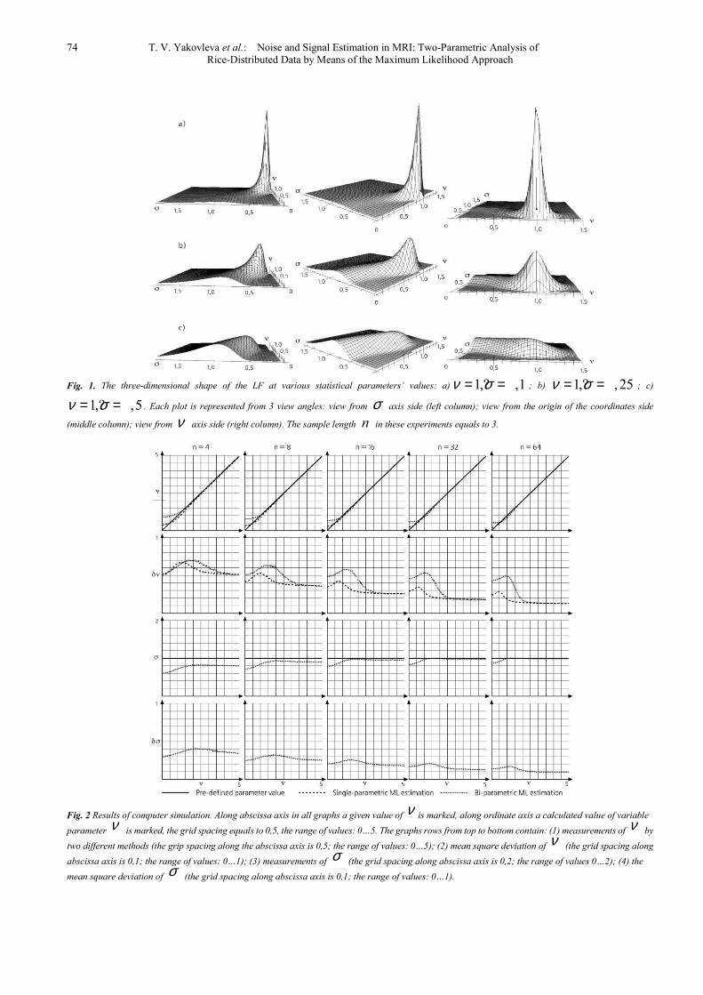
The example plots of the LF shape presented in Fig. 1 for

various signal-to-noise ratio values may illustrate the

uniqueness of the two-parametric ML equations’ solution.

Based upon the assumption, that the two-parametric ML

equations’ solution is unique, we proved the following

assertion:

Theorem 3

The unique non-zero solution of the equation (14) always

corresponds to the global maximum of the LLF (11).

This conclusion may seem to be unexpected as from

Theorem 1 it follows that the ML estimation may take the

place at 0ν = (what in our case would correspond to zero

value of variable γ and uncertain value of σ ).

Nevertheless this paradox is only the seeming one and may

be explained as follows. The zero estimation of variable ν

is possible only at a priory known value of σ (let us denote

it asA

σ ). However in our case we use the value of σ

having been obtained by means of solving the maximum

likelihood equation (we shall denote it asML

σ ). At such a

value of σ the mean value parameter ν can be infinitely

close to zero, but cannot be equal strictly to zero.

5. Two-Parametric ML Problem:

Practical Issues

The numerical solution of the equation (14) allows

finding the value of the parameter2

νγσ

= , and then, taking

into account expression (13), determining the values of the

parameters ν and σ as well.

It is worth mentioning, that the proposed solution of the

system (13) demonstrates a new meaning of the

“conventional” estimation of the parameterν , provided by

the formula

2 22 Axν σ= − , (15)

where2

Aσ is some hypothetic value specified a priori. In

the paper [11] this formula was subjected to some just

criticism due to the following issues:

1. It loses the sense at 2 22A

x σ< ;

2. It does not provide a strict estimation of the parameter

from the viewpoint of the ML principle.

However, if we substitute the first equation of the system

(13) into the second one with replacing the function S by

ν and the parameter γ by2ν σ , we obtain the following

expression coinciding with the conventional estimation

formula:

2 22 MLxν σ= − (16)


where ML

σ means the estimation of the parameter σ ,

having been obtained as a result of the solution of the

equations’ system (13), i. e. corresponding to the maximum

of the LF. Despite the fact that this formula looks exactly as

a conventional one, one can affirm that just this formula

provides the ML estimation for the parameter ν if the

parameter σ was not taken as a priory known A

σ but was

calculated by means of the ML equations’ system (13)

solving.

So, from the above analysis the conclusion follows that

the system (13) always has a nontrivial solution and so the

situation 2 22ML

x σ< never takes place. The calculation by

the formula (16) always provides the ML estimation.

Subsequently, we obtain the following optimal strategy of

this method application:

1. By means of the numerical solution of the equations’

system (13) a parameter 2

MLσ is calculated for some

homogeneous area of an image;

2. All other calculation are conducted by the formula (16)

and do not demand a numerical solution of any equations.

The elaborated procedure allows accurate ML estimating

of the statistical parameters of an image, based upon the

measured data instead of any a priory assumptions. The

obtained values of the parameters correspond to the

maximum of the LF. This technique is not associated with

cumbersome computing as the principle calculations are

implemented by means of a simple formula (16).

6. The Numerical Simulation Results

The both above described ML approaches were tested by

means of computer simulation (one- and two-parametric).

The first numerical experiment was conducted as follows.

The data were generated obeying to the Rice distribution

with the parameters given beforehand. Parameter σ was

assumed to be equal to 1, while parameter ν was changed

from 0 to 5. So created sets were used to make measures of

the parameters according to the above presented algorithms.

The experiments were performed at variable sample’s length

n : from 4 up to 64. The same experiment for each value of

ν , σ and n was repeated 410 times to acquire statistics.

For each n four types of measurements were

implemented:

1. Calculation of parameter ν by means of the ML

method:

• traditional one-parametric ML estimation of ν by

means of solving (8) assuming that parameter σ is known

a priory;

• original two-parametric ML estimation according to (13)

for the case when both statistical parameters are unknown.

These results are presented by an upper row of the graphs

in Fig. 2.

2. Calculation of the mean square deviation of the

measured values of parameter ν for both methods. These

results are presented by the second from top row of the

graphs in Fig. 2.

3. Calculation of parameter σ by means of the ML

method: only two-parametric estimation according the

equations (13). The results are presented by the third from

top row of graphs in Fig. 2.

4. Definition of the mean square deviation of the

measured values of parameter σ . These results are

presented by lower row of the graphs in Fig.2.

On the basis of the presented graphs were have

investigated the errors inherent to both one-parametric and

two-parametric methods. The results are compiles in Table 1

.Table 1. Investigated methods’ errors estimation

Parameter Error type, measurement method n=4 n=8 n=16 n=32 n=64

ν

Maximum systematic bias, one-parametric method (σ is known a priory) 0,4 0,35 0,3 0,25 0,2

Maximum systematic bias, two-parametric method (σ is found from the sample) 0,9 0,8 0,7 0,6 0,5

Maximum mean square deviation, one-parametric method (σ is known a priory) 0,68 0,63 0,58 0,53 0,49

Maximum mean square deviation, two-parametric method (σ is found from the sample) 0,7 0,53 0,42 0,35 0,18

σ

Maximum systematic bias at small ν –0,4 –0,39 –0,21 –0,16 –0,12

Asymptotic systematic bias of σ estimation at large ν –0,2 –0,1 –0,04 –0,02 –0,01

Maximum mean square deviation at small ν 0,4 0,33 0,26 0,21 0,17

Asymptotic mean square deviation at large ν 0,3 0,25 0,18 0,13 0,09



Fig. 1. The three-dimensional shape of the LF at various statistical parameters’ values: a) 1,? ,1ν σ= = ; b) 1,? ,25ν σ= = ; c)

1,? ,5ν σ= = . Each plot is represented from 3 view angles: view from σ axis side (left column); view from the origin of the coordinates side

(middle column); view from ν axis side (right column). The sample length n in these experiments equals to 3.

Fig. 2 Results of computer simulation. Along abscissa axis in all graphs a given value of ν is marked, along ordinate axis a calculated value of variable

parameter ν is marked, the grid spacing equals to 0,5, the range of values: 0…5. The graphs rows from top to bottom contain: (1) measurements of ν by

two different methods (the grip spacing along the abscissa axis is 0,5; the range of values: 0…5); (2) mean square deviation of ν (the grid spacing along

abscissa axis is 0,1; the range of values: 0…1); (3) measurements of σ (the grid spacing along abscissa axis is 0,2; the range of values 0…2); (4) the

mean square deviation of σ (the grid spacing along abscissa axis is 0,1; the range of values: 0…1).


As it follows from the data of Table 1, with the growth of

the amount of the data points in a sample an error at

computing the statistical parameters decreases noticeably

(especially the mean square deviation).

Table 1 and Fig. 2 make clear the important peculiarity of

the Rician distribution: both bias and variance of the

measured ν values grow strongly at low SNR, which is

inherent to both variants of the examined ML estimation

procedures. This can be explained with the aid of Fig. 1 plots:

one can see, that the less is SNR, the less expressed is the

maximum of LF. Nevertheless, this maximum never

disappears completely.

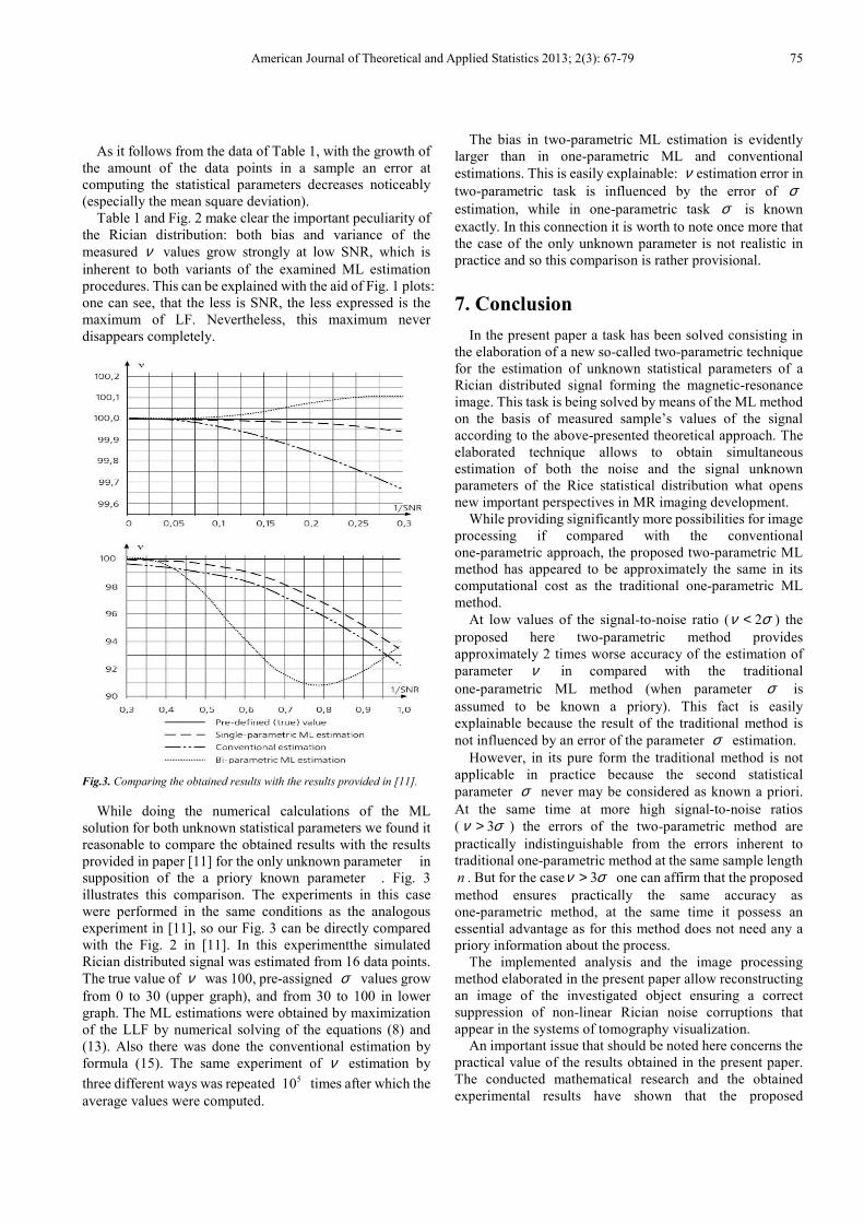
Fig.3. Comparing the obtained results with the results provided in [11].

While doing the numerical calculations of the ML

solution for both unknown statistical parameters we found it

reasonable to compare the obtained results with the results

provided in paper [11] for the only unknown parameter in

supposition of the a priory known parameter . Fig. 3

illustrates this comparison. The experiments in this case

were performed in the same conditions as the analogous

experiment in [11], so our Fig. 3 can be directly compared

with the Fig. 2 in [11]. In this experimentthe simulated

Rician distributed signal was estimated from 16 data points.

The true value of ν was 100, pre-assigned σ values grow

from 0 to 30 (upper graph), and from 30 to 100 in lower

graph. The ML estimations were obtained by maximization

of the LLF by numerical solving of the equations (8) and

(13). Also there was done the conventional estimation by

formula (15). The same experiment of ν estimation by

three different ways was repeated 510 times after which the

average values were computed.

The bias in two-parametric ML estimation is evidently

larger than in one-parametric ML and conventional

estimations. This is easily explainable: ν estimation error in

two-parametric task is influenced by the error of σ

estimation, while in one-parametric task σ is known

exactly. In this connection it is worth to note once more that

the case of the only unknown parameter is not realistic in

practice and so this comparison is rather provisional.

7. Conclusion

In the present paper a task has been solved consisting in

the elaboration of a new so-called two-parametric technique

for the estimation of unknown statistical parameters of a

Rician distributed signal forming the magnetic-resonance

image. This task is being solved by means of the ML method

on the basis of measured sample’s values of the signal

according to the above-presented theoretical approach. The

elaborated technique allows to obtain simultaneous

estimation of both the noise and the signal unknown

parameters of the Rice statistical distribution what opens

new important perspectives in MR imaging development.

While providing significantly more possibilities for image

processing if compared with the conventional

one-parametric approach, the proposed two-parametric ML

method has appeared to be approximately the same in its

computational cost as the traditional one-parametric ML

method.

At low values of the signal-to-noise ratio ( 2ν σ< ) the

proposed here two-parametric method provides

approximately 2 times worse accuracy of the estimation of

parameter ν in compared with the traditional

one-parametric ML method (when parameter σ is

assumed to be known a priory). This fact is easily

explainable because the result of the traditional method is

not influenced by an error of the parameter σ estimation.

However, in its pure form the traditional method is not

applicable in practice because the second statistical

parameter σ never may be considered as known a priori.

At the same time at more high signal-to-noise ratios

( 3ν σ> ) the errors of the two-parametric method are

practically indistinguishable from the errors inherent to

traditional one-parametric method at the same sample length

n . But for the case 3ν σ> one can affirm that the proposed

method ensures practically the same accuracy as

one-parametric method, at the same time it possess an

essential advantage as for this method does not need any a

priory information about the process.

The implemented analysis and the image processing

method elaborated in the present paper allow reconstructing

an image of the investigated object ensuring a correct

suppression of non-linear Rician noise corruptions that

appear in the systems of tomography visualization.

An important issue that should be noted here concerns the

practical value of the results obtained in the present paper.

The conducted mathematical research and the obtained

experimental results have shown that the proposed



two-parametric technique can be reliably applied for the

image analysis tasks at rather high values of signal-to-noise

ratios ( 3ν σ> ). We expect the possible opponents’

objections that at high values of signal-to-noise ratios these

is no need to use elaborated two-parametric approach to

solve the tasks within the Rice statistical model as at this

area the Gauss distribution can be applied. But such kind of

objection would be not true due to the following reasons: the

Gauss distribution starts properly working for the

considered task at significantly higher values of

signal-to-noise ratio, namely: at 10ν σ> . So, there is a large

interval of practically meaningful signal values

10 3σ ν σ> > in magnetic-resonance imaging which is

adequately described by the Rician statistical model. And in

this interval the elaborated two-parametric technique seems

to be the most appropriate for describing and calculating the

image processing tasks making use of all the advantages of

this technique provided above.

In the conclusion it is worth to underline that the present

paper provides a theoretical analysis of the maximum

likelihood method for the two-parametric task in the Rician

distributed image processing. The developed

two-parametric version of the maximum likelihood method

is a new effective tool both to process the Rician images and

to evaluate the precision of other two-parametric techniques

by comparing with the technique proposed in the present

paper.

A principle merit of the elaborated technique consists in

the proved possibility to obtain the unique values of both

major statistical parameters of the image at the “cost” of

one-parameter estimation.

Appendix. Proofs of Principle

Statements

Lemma 1

Function ( )I zɶ is positive-valued, monotonically

increasing and concave at interval ( )0,+∞ .

Proof:

The condition of monotonic character of the function

( )I zɶ means the nonnegativity of its derivative. Taking into

account the definition of the function ( )I zɶ and the known

formula ( ) ( )0 1I z I z′ = we can put down its derivative as

follows:

( ) ( ) ( ) ( ) ( )( )

( ) ( ) ( )( )

1 0 1 0

2

0

2

0 1 1

2

0

I z I z I z I zI z

I z

I z I z I z

I z

′ ′−′ =

′⋅ −=

ɶ

(17)

The function 0

I in the denominator is always positive,

so the sign of the derivative of function ( )I zɶ is determined

by the sign of (17) numerator. So to prove the monotonic

character of the function ( )I zɶ , i.e. the nonnegativity of its

derivative, it is sufficient to prove the nonnegativity of the

numerator of (17) at 0z ≥ .

Let us consider the known integral presentation of the

modified Bessel function of the first kind of integer order:

( ) cos

0

1cosz

nI z e n d

πθ θ θ

π= ∫ (18)

where ( ),Il z∈ >Z . From this formula we can obtain

the following expressions for functions ( )0I z and ( )1

I z :

( ) cos

0

0

1 z tI z e dt

π

π= ∫ , ( ) cos

1

0

1cosz tI z e tdt

π

π= ⋅∫ (19)

Similarly, for the derivative of the function ( )1I z we

obtain:

( ) cos 2

1

0

1cosz tI z e tdt

π

π′ = ∫ (20)

Substituting (19) and (20) into the numerator of the

expression (18) we get:

( ) ( ) ( )2

1 0 1

cos 2 cos

2

0 0

cos cos

2

0 0

1cos

1cos cos

z t z t

z t z t

I z I z I z

e tdt e dt

e tdt e t dt

π π

π π

π

π

′

′

′ − =

′⋅ −

′ ′− ⋅

∫ ∫

∫ ∫

(21)

As a result of non-complicated transforms we obtain for

the expression (21) the following view:

( ) ( ) ( )( ) ( )

2

1 0 1

2cos cos

2

0 0

1cos cos

2

z t t

I z I z I z

dtdt e t t

π π

π′+

′ ⋅ − =

′ ′−∫ ∫ (22)

By virtue of nonnegative value of the sub-integral

expression it obviously follows from (22) that the whole

expression (22) is nonnegative and, consequently, the

derivative of function ( )I zɶ is nonnegative, what means its

monotony at 0z ≥ . So the function’s monotony is proved.

The proof of concavity is implemented similarly,

although it demands much more cumbersome calculations.

Lemma 2

( )0Iz I z∀ > ∈ɶ (0,1)

Proof:


Let us consider the integral representation (18). At 0n =

the sub-integral expression is always larger than the same

expression at 1n = . From this fact it easily follows that:

( ) ( )0 10Iz I z I z∀ > > . The lemma is proved.

Theorem 1

Let us suppose that the condition 2 22x σ> is valid.

Then at 0ν > there exists a unique solution of equation (8),

which corresponds to the LF maximum. If 2 22x σ≤ , then

the LF maximum corresponds to trivial solution of equation

(8), i.e. to 0ν = .

Proof:

To determine the conditions of the existence of non-trivial

solution of equation (8) let us consider the behavior of the

right and the left parts of this equation.

The left part of equation (8) is presented by a straight line

1y ν= . The right part, as it follows from the properties of

function ( )I zɶ , having been proved in Lemma 1, is presented

by a smooth monotonic concave function

( )2 21

1 ni

i

i

xy I x

n

ννσ=

= ⋅

∑ ɶ . The graph of this function is a

curve passing through the coordinates origin point and

asymptotically approaching to the straight line y x= . Due

to its concave character this curve can have one or two

common points with the straight line 1y ν= . One of these

points is always known to us and corresponds to the trivial

solution 0ν = .

The existence of the second common point is determined

by the function ( )2y ν derivative in the vicinity of the

coordinates’ origin point: for the existence of the second

solution it is necessary and sufficient that the condition

( ) ( )2 10 0 1y y′ ′< = takes place. Let us find the derivative

( )20y′ :

( ) ( )2

2 21

1 ni

i

i i

xy I z

n zν

σ=

∂′ = ⋅∂∑ ɶ

where2

ii

xz

νσ

=. We shall use the known formulas of the

decomposition into a series [20]:

( ) ( ) ( ) ( )( )

2 2 1

0 1

0 0

2 2,

! ! ! 1 !

k k

k k

z zI z I z

k k k k

+∞ ∞

= =

= =⋅ ⋅ +∑ ∑ (23)

From decompositions (23) we obtain the following

formula describing the behavior of function ( )I zɶ at

0z → :

( ) ( )2

412 8

z zI z O z

⋅ − +

ɶ ≃

Taking into account this estimation of the function ( )I zɶ

at small values of argument, we obtain:

( )2

2 2

1

10

2

ni

i

xy

n σ=

′ = ∑ (24)

Thus, the non-trivial solution of equation (8) exists only at

the condition 2 22x σ> . To determine if any solution of

equation (8) corresponds to maximum or to minimum of the

LF we have to consider the second derivative of the LLF.

From equation (5) taking into account expressions (6) and

(7), we obtain:

( ) ( ) ( )2

1 22ln ,L y yν σ ν ν

ν∂ ′ ′= −

∂

In the vicinity of zero this expression can be transferred

into the following one:

( )2

2 2

2ln , 1 2L xν σ σ

ν∂ = −

∂.

So, at 2 22x σ> the second derivative in the vicinity of

zero is positive what corresponds to the minimum of the

LLF. Since the LLF and all its derivatives are smooth, its

second extremum at 0ν > can be only a maximum. At 2 22x σ< the second derivative in the vicinity of zero is

negative and this means that the LLF has a maximum. So the

theorem is proved.

Theorem 2

The solution of the equation (14) for non-negative values

of the parameter γ exists.

Proof:

Let us consider equation (14) at 0γ ≥ , what corresponds

to the physical sense of the task. Then the left part of

equation (14) is presented by a straight line ( )3y γ γ= ,

passing through the coordinates’ origin point. Let us

consider the behavior of the equation’s right part:

( ) ( )( )4 2 2

2 Sy

x S

γγ

γ=

−

The denominator of this expression is positive

monotonically decreasing function by virtue of lemmas 1

and 2 while the nominator is a positive monotonically

increasing function. So the function itself is monotonically

increasing.

Taking into account the series decomposition formulas

(23), we obtain the following expression, which is valid at

vanishing values of variable γ :

( )2

2

40

lim 14

xy

γγ γ γ γ

→

= ⋅ + >



Thus in the vicinity of zero value of variable γ the curve

( )4y γ , displaying the right part of equation (14), goes

above the straight line corresponding to the left part of this

equation: ( )3y γ γ= .

At larger values of variable γ the right part of equation

(14), by virtue of the asymptotic behavior of the modified

Bessel functions, can be put down as follows:

( )4 22

2lim 0

xy

x xγγ

→ ∞= >

− (25)

It is easily seen that the denominator of expression (25) is

a non-negative magnitude and equals to mean squared

deviation of a sample valuei

x . So with increasing the value

of variable γ the right part of equation (14) asymptotically

approaches to the constant positive value determined by

expression (25). This means that the curve corresponding to

the right part of equation (14) inevitably crosses the straight

line corresponding to the left part of this equation because in

the vicinity of zero this curve goes above the mentioned

straight line. In other words, from the above considerations

we can conclude that the non-trivial solution of equation (14)

exists. The theorem is proved.

Theorem 3

The unique solution of the equation (14) corresponds to

the global maximum of the LLF (11).

Proof:

Let us find the second derivative of the ( )ln ,L ν γ⌢

function with respect to γ :

( ) ( )( )

22

2

2

2 2

1 1ln ,

2 2

1

2 2

xSL

n S

S Sx

S

γν γ

γ γγ

γ

′ ∂ = + − ∂

′ ′= − + +

⌢

Making use of expressions having been obtained by us

while proving the Theorem 1, we get the following

estimation at 0γ → :

( )2 32

2 20

1 1lim ln ,

4 16

x xL

n xγν γ

γ→

∂ = +∂

⌢

,

This means that the second derivative of the LLF is

always positive at zero point and consequently this point

corresponds to its minimum. As the LLF is smooth, its

second extreme point can be only a maximum.

References

[1] T. Wang and T. Lei, “Statistical analysis of MR imaging and its application in image modeling,” in Proc. IEEE Int. Conf.

Image Processing and Neural Networks, vol. I, 1994, pp. 866–870.

[2] S. O. Rice, “Mathematical analysis of random noise,” Bell Syst. Technological J., vol. 23, p. 282, 1944.

[1] R. M. Henkelman, “Measurement of signal intensities in the presence of noise in MR images”. Med. Phys., vol. 12, no. 2, pp. 232–233, 1985.

[2] A. Papoulis, Probability, Random Variables and Stochastic Processes, 2nd ed. Tokyo, Japan: McGraw-Hill, 1984.

[3] H. Gudbjartsson and S. Patz, “The Rician distribution of noisy MRI data”, Magn. Reson. Med., vol.34, pp.910—914, 1995.

[4] A. Macovski, “Noise in MRI”, Magn. Reson. Med., vol. 36, No.3, pp.494—497, 1996.

[5] G. Gerig, O. Kubler, R. Kikinis, and F. A. Jolesz, “Nonlinear anisotropic filtering of MRI data,” IEEE Trans. Med. Imag., vol. 11, pp. 221–232, June 1992.

[6] G. Z. Yang, P. Burger, D. N. Firmin, and S. R. Underwood, “Structure adaptive anisotropic filtering for magnetic resonance image enhancement,” in Proc. CAIP, pp. 384–391, 1995.

[7] S. J. Garnier and G. L. Bilbro, “Magnetic resonance image restoration,” J. Math. Imag., Vision, vol. 5, pp. 7—19, 1995.

[8] G. McGibney and M. R. Smith, “An unbiased signal-to-noise ratio measure for magnetic resonance images,” Med. Phys., vol. 20, no. 4,pp. 1077—1078, 1993.

[9] Jan Sijbers, Arnold J. den Dekker, Paul Scheunders, and Dirk Van Dyck, “Maximum-Likelihood Estimation of Rician Distribution Parameters”, IEEE Transactions on Medical Imaging, vol.17, No 3, p.p. 357—361, June 1998.

[10] Jeny Rajan, Ben Jeurissen, Marleen Verhoye, Johan Van Audekerke and Jan Sijbers, “Maximum likelihood estimation based denoising of magnetic resonance images using restricted local neighborhoods”. Physics in Medicine and Biology, vol. 56, issue 16, pp. 2011. DOI: 10.1088/0031-9155/56/16/009

[11] Jeny Rajan, Dirk Poot, Jaber Juntu and Jan Sijbers, “Noise measurement from magnitude MRI using local estimates of variance and skewness”, Phys. Med. Biol. 55, p.p.441–449, 2010.

[12] J. Sijbers & A. J. den Dekker, “Maximum Likelihood estimation of signal amplitude and noise variance from MR data”. Magn Reson Med 51(3):586—594, 2004.

[13] L. He & I. R. Greenshields , “A Nonlocal Maximum Likelihood Estimation Method for Rician Noise Reduction in MR images”. IEEE Trans Med Imaging 28:165—172, 2009.

[14] Aja-Fernandez, S.; Alberola-Lopez, C.; Westin, C.-F. Noise and Signal Estimation in Magnitude MRI and Rician Distributed Images: A LMMSE Approach // IEEE Transactions on Image Processing, vol. 17, issue 8, pp. 1383—1398, 2008.

[15] C. F.M. Carobbi, M. Cati, “The absolute maximum of the likelihood function of the Rice distribution:existence and uniqueness, IEEE Trans. on Instrumentation and Measurement, vol 57, No 4, April 2008, pp. 682-689.


[16] Rytov, S.М. Introduction into Statistical Radio-physics. P.1. Random processes. — Мoscow: Nauka, 1976 (in Russian).

[17] P.J.Bickel, K.A.Doksum, Mathematical Statistics, Holden-Day, Inc., 1983.

[18] М. Abramowitz and I. Stegun (eds.) Handbook of Mathematical Functions with formulas, graphics and mathematical tables. National Bureau of Standards, applied mathematics series-55; Issued June 1964.

[19] T. Yakovleva. “Two-parametric method of noise and signal determination in magnetic resonance imaging: mathematical substantiation”, unpublished.

[20] Young, Phillip M., et al. "MR imaging findings in 76 consecutive surgically proven cases of pericardial disease with CT and pathologic correlation." The international journal of cardiovascular imaging 28.5 (2012): 1099-1109.

[21] Samarin, Andrei, et al. "PET/MR imaging of bone lesions–implications for PET quantification from imperfect attenuation correction." European journal of nuclear medicine and molecular imaging 39.7 (2012): 1154-1160.

[22] Hualong Zu, Qixin Wang, Mingzhi Dong,Liwei Ma, Liang Yin, Yanhui Yang. “Compressed Sensing Based Fixed-Point DCT Image Encoding”, Advances in Computational Mathematics and its Applications, 2.2 (2012): 259-262

Documents

Noise and signal estimation in MRI: two-parametric analysis of rice …article.sciencepublishinggroup.com/pdf/10.11648.j.ajtas.20130203... · Noise and signal estimation in MRI: two-parametric