Node Overlap Removal by Growing a Tree - arXiv.org e … · Node Overlap Removal by Growing a Tree ... Node overlap removal is a necessary step in many scenarios ... by an axis-aligned

Node Overlap Removal by Growing a Tree

Lev Nachmanson1, Arlind Nocaj2, Sergey Bereg3, Leishi Zhang4, andAlexander Holroyd1

1Microsoft Research, Redmond, USA2University of Konstanz, Konstanz, Germany

3The University of Texas at Dallas, Richardson, USA4Middlesex University, London,UK

[email protected], [email protected], [email protected],

[email protected], [email protected]

Abstract. Node overlap removal is a necessary step in many scenariosincluding laying out a graph, or visualizing a tag cloud. Our contributionis a new overlap removal algorithm that iteratively builds a MinimumSpanning Tree on a Delaunay triangulation of the node centers and re-moves the node overlaps by ”growing” the tree. The algorithm is simpleto implement yet produces high quality layouts. According to our ex-periments it runs several times faster than the current state-of-the-artmethods.

1 Introduction

Removing node overlap after laying out a graph is a common task in networkvisualization. Most graph layout algorithms [23] consider nodes as points that donot occupy any geometrical space. In practice, nodes often have shapes, labels,and so on. These shapes and labels may overlap in the visualization and affectthe visual readability. To remove such overlaps a specialized algorithm is usuallyapplied.

The main contribution of this paper is a new node overlap removal algorithmthat we call Growing Tree, or GTree further on. The basic idea is to first capturemost of the overlap and the local structure with a specific spanning tree on topof a proximity graph, and then resolve the overlap by letting the tree ”grow”.

We compare GTree with PRISM [6], which is widely used for the same pur-pose. Needing more area than PRISM, our method preserves the original layoutwell and is up to eight times faster than PRISM. To compare the two algo-rithms we implemented GTree in the open source graph visualization softwareGraphviz 1, where PRISM is the default overlap removal algorithm. On the otherside, GTree is the default in MSAGL2, where we also have an implementationof PRISM. We ran comparisons by using both tools.

1 http://www.graphviz.org/2 https://github.com/Microsoft/automatic-graph-layout

arX

iv:1

608.

0265

3v1

[cs

.CG

] 8

Aug

201

6

http://www.graphviz.org/

2 Related Work

There is vast research on node overlap removal. Some methods, including hierar-chical layouts [4], incorporate the overlap removal with the layout step. Likewise,force-directed methods [5] have been extended to take the node sizes into ac-count [16, 17, 24], but it is difficult to guarantee overlap-free layouts withoutincreasing the repulsive forces extensively. Dwyer et al. [2] show how to avoidnode overlaps with Stress Majorization [7]. The method can remove node over-laps during the layout step, but it needs an initial state that is overlap free;sometimes such a state is not given.

Another approach, which we also choose, is to use a post-processing step. InCluster Busting [8, 18] the nodes are iteratively moved towards the centers oftheir Voronoi cells. The process has the disadvantage of distributing the nodesuniformly in a given bounding box.

Imamichi et al. [15] approximate the node shapes by circles and minimize afunction penalizing the circle overlaps.

Starting from the center of a node, RWorldle [22] removes the overlaps bydiscovering the free space around a node by using a spiral curve and then utilizingthis space. The approach requires a large number of intersection queries that aretime consuming. This idea is extended by Strobelt et al. [21] to discover availablespace by scanning the plane with a line or a circle.

Another set of node overlap removal algorithms focus on the idea of definingpairwise node constraints and translating the nodes to satisfy the constraints [11,13, 19, 20]. These methods consider horizontal and vertical problems separately,which often leads to a distorted aspect ratio [6]. A Force-transfer-algorithm isintroduced by Huang et al. [14]; horizontal and vertical scans of overlapped nodescreate forces moving nodes vertically and horizontally; the algorithm takesO(n2)steps, where n is the number of the nodes. Gomez et al. [9] develop Mixed IntegerOptimization for Layout Arrangement to remove overlaps in a set of rectangles.The paper discusses the quality of the layout, which seems to be high, but notthe effectiveness of the method, which relies on a mixed integer problem solver.Dwyer et al. [3] reduce the overlap removal to a quadratic problem and solve itefficiently in O(n log n) steps. According to Gansner and Hu [6], the quality andthe speed of the method of Dwyer et al. [3] is very similar to the ones of PRISM.

The ProjSnippet method [10] generates good quality layouts. The methodrequires O(n2) amount of memory, at least if applied directly as described in thepaper, and the usage of a nonlinear problem solver.

In PRISM [6, 12], a Delaunay triangulation on the node centers is used as thestarting point of an iterative step. Then a stress model for node overlap removalis built on the edges of the triangulation and the stress function of the modelis minimized. GTree also starts with building this Delaunay triangulation, butthen the algorithms diverge.

3 GTree Algorithm

An input to GTree is a set of nodes V , where each node i ∈ V is representedby an axis-aligned rectangle Bi with the center pi. We assume that for differenti, j ∈ V the centers pi, pj are different too. If this is not the case, we randomlyshift the nodes by tiny offsets. We denote by D a Delaunay triangulation of theset {pi : i ∈ V }, and let E be the set of edges of D.

On a high level, our method proceeds as follows. First we calculate the tri-angulation D, then we define a cost function on E and build a minimum costspanning tree on D for this cost function. Finally, we let the tree “grow”. Thesteps are repeated until there are no more overlaps. The last several steps areslightly modified. Now we explain the algorithm in more detail.

We define the cost function c on E in such a way that the larger the overlapon an edge becomes, the smaller the cost of this edge comes to be. Let (i, j) ∈ E.If the rectangles Bi and Bj do not overlap then c(i, j) = dist(Bi, Bj), that isthe distance between Bi and Bj . Otherwise, for a real number t let us denote byBj(t) a rectangle with the same dimensions as Bj and with the same orientation,but with the center at pi+ t(pj−pi). We find tij > 1 such that the rectangles Biand Bj(tij) touch each other. Let s = ‖pj − pi‖, where ‖‖ denotes the Euclideannorm. We set c(i, j) = −(tij − 1)s. See Figure 1 for an illustration.

pi

pjs d d = tijs

cij = s− doverlapping nodes

Bi

Bj

dist(Bi, Bj)

cij = dist(Bi, Bj)

non overlapping nodes

Fig. 1: Cost function cij for edges of the Delaunay triangulation. For overlappingnodes −cij is equal to the minimal distance that is necessary to shift the boxesalong the edge direction so they touch each other.

Having the cost function ready, we compute a minimum spanning tree T onD. Remember that it is a tree with the set of vertices V for which the cost,∑e∈E′ c(e), is minimal, where E′ is the set of edges of the tree. We use Prim’s

algorithm to find T .The algorithm proceeds by growing T , similar to the growth of a tree in

nature. It starts from the root of T . For each child of the root overlapping withthe root, it extends the edge connecting the root and the child to remove theoverlap. To achieve this, it keeps the root fixed but translates the sub-tree of thechild. The edges between the root and other children remain unchanged. Thealgorithm recursively processes the children of the root in the same manner. Thisprocess is described in Algorithm 1.

The number tij in line 5 of Algorithm 1 is the same as in the definition ofthe cost of the edge (i, j) when Bi and Bj overlap, and is 1 otherwise.

Algorithm 1: Growing T

Input: Current center positions p and root rOutput: New center positions p′

1 p′r = pr2 GrowAtNode (r)3 function GrowAtNode (i)4 foreach j ∈ Children(i) do5 p′j = p′i + tij(pj − pi)6 GrowAtNode (j);

The algorithm does not update all positions for the child sub-tree nodesimmediately, but updates only the root of the sub-tree. Using the initial positionsof a parent and a child, and the new position of the parent, the algorithm obtainsthe new position of the child in line 5. In total, Algorithm 1 works in O(|V |)steps. The choice of the root of the tree does not matter. Different roots producethe same results modulo a translation of the plane by a vector. Indeed it can be

(a) iteration 1 (b) iteration 2 (c) iteration 3

(d) iteration 4 (e) iteration 5(f) final overlap free graphwith original shapes

Fig. 2: Overlap removal process with the minimum spanning tree on the proxim-ity graph, where the latter here is a Delaunay triangulation on rectangle centers.The blue edges form a tree; there are four different trees in the figure. The treeedges connecting overlapped nodes are thick and solid. In each iteration thethick edges are elongated and the dashed tree edges shift accordingly. Overlapis completely resolved in four iterations.

shown that after applying the algorithm, for any i, j ∈ V the vector p′j − p′i isdefined uniquely by the path from i to j in T .

While an overlap along any edge of the triangulation exists, we iterate, start-ing from finding a Delaunay triangulation, then building a minimum spanningtree on it, and finally running Algorithm 1. See Figure 2 for an example.

When there are no overlaps on the edges of the triangulation, as noticedby Gansner and Hu [6], overlaps are still possible. We follow the same idea asPRISM and modify the iteration step. In addition to calculating the Delaunaytriangulation we run a sweep-line algorithm to find all overlapping node pairsand augment the Delaunay graph D with each such a pair. As a consequence,the resulting minimum spanning tree contains non-Delaunay edges catching theoverlaps, and the rest of the overlaps are removed. This stage usually requiresmuch less time than the previous one.

It is possible to create an example where the algorithm will not remove alloverlaps. However, such examples are extremely rare and have not been seen yetin practice of using MSAGL or in our experiments. MSAGL applies random tinychanges to the initial layout which prevents GTree from cycling.

4 Comparing PRISM and GTree by Measuring LayoutSimilarity, Quality, and Run Time

Our data includes the same set of graphs that was used by the authors of PRISMto compare it with other algorithms [6]. The set is available in the Graphvizopen source package3. We also used a small collection of random graphs and acollection of about 10,000 files4. For the experiments we use a modified versionof Dot, where we can invoke either GTree or Prism for the overlap removal step,and we also used MSAGL, where we implemented PRISM and GTree. MSAGLwas used only to obtain the quality measures. We ran the experiments on a PCwith Linux, 64bit and an Intel Core i7-2600K [email protected] with 16GB RAM.

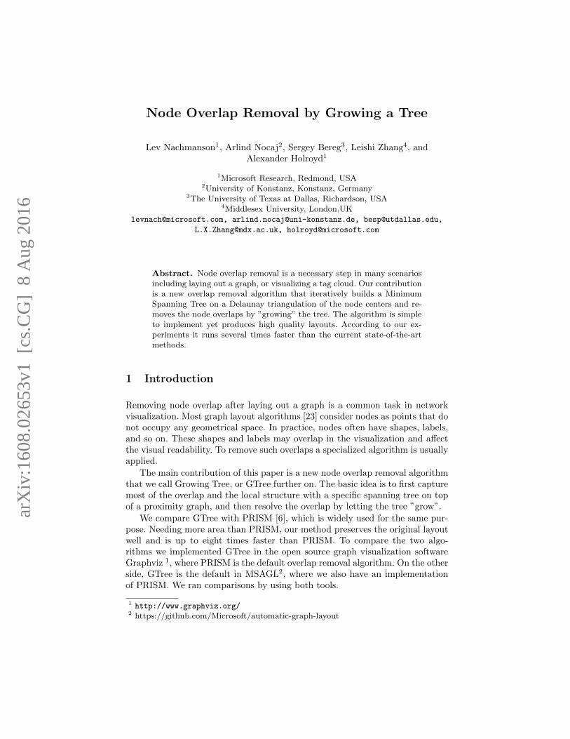
Some of resulting layouts can be seen in Figures 3, 5, 6.One can try to resolve overlap by scaling the node centers of the original

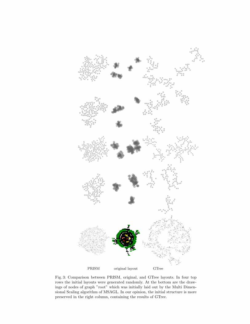
layout. If there are no two coincident node centers this will work, but the resultinglayout may require a huge area if some centers are close to each other. Weconsider the area of the final layout as one of the quality measures, and usuallyPRISM produces a smaller area than GTree, see Table 1.

In addition to comparing the areas, we compare some other layout properties.Following Gansner and Hu [6], we look at edge length dissimilarity, denoted asσedge. This measure reflects the relative change of the edge lengths of a DelaunayTriangulation on the node centers of the original layout.

The other measure, which is denoted by σdisp, is the Procrustean similar-ity [1]. It shows how close the transformation of the original graph is to a com-bination of a scale, a rotation, and a shift transformation. PRISM and GTreeperforms similar in the last two measures as Table 1 shows.

3 http://www.graphviz.org4 https://www.dropbox.com/sh/4q0k89yrv4x3ae3/AAA3xyKFRhLyyHXcG9jpcgata?dl=0

PRISM original layout GTree

Fig. 3: Comparison between PRISM, original, and GTree layouts. In four toprows the initial layouts were generated randomly. At the bottom are the draw-ings of nodes of graph ”root” which was initially laid out by the Multi Dimen-sional Scaling algorithm of MSAGL. In our opinion, the initial structure is morepreserved in the right column, containing the results of GTree.

To distinguish the methods further, we measure the change in the set of kclosest neighbors of the nodes. Namely, let p1, . . . , pn be the positions of thenode centers, and let k be an integer such that 0 < k ≤ n. Let I = {1, . . . , n}be the set of node indices. For each i ∈ I we define Nk(i) ⊂ I \ {i}, suchthat |Nk(p, i)| = k, and for every j ∈ I \ Nk(p, i) and for every j′ ∈ Nk(p, i)holds ‖pj − pi‖ ≥ ‖pj′ − pi‖. In other words, Nk(p, i) represents a set of kclosest neighbors of i, excluding i. Let p′1, . . . , p

′n be transformed node centers.

To see how much the layout is distorted nearby node i, we intersect Nk(p, i)and Nk(p′, i). We measure the distortion as (k−m)2, where m is the number ofelements in the intersection. One can see that if the node preserves its k closestneighbors then the distortion is zero.

Our experiments for k from 8 to 12 show that under this measure GTreeproduced a smaller error, showing less distortion, on 8 graphs from 14, and onthe rest PRISM produced a better result, see Table 2. GTree produced a smallererror on all small random graphs from other collections5.

Table 1: Similarity to the initial layout (left) and number of iterations for dif-ferent graph sizes and different initialization methods (right). PR stands forPRISM

σedge σdisp areaGraph PR GTree PR GTree PR GTree

dpd 0.34 0.28 0.37 0.36 0.82 0.84unix 0.22 0.19 0.24 0.20 2.38 2.38rowe 0.29 0.26 0.23 0.24 0.68 0.73size 0.39 0.37 0.24 0.26 1.09 1.28ngk10 4 0.30 0.30 0.27 0.30 0.00 0.00NaN 0.56 0.44 0.73 0.51 4.03 4.34b124 0.55 0.53 0.97 0.83 5.52 6.22b143 0.67 0.70 1.12 0.93 3.62 3.88mode 0.54 0.50 0.59 0.53 1.53 2.29b102 0.71 0.77 1.43 1.27 4.50 6.62xx 0.75 0.70 1.65 1.42 6.21 9.57root 1.09 1.19 2.89 2.45 34.58 91.87badvoro 0.88 0.92 2.27 2.42 25.68 47.43b100 0.84 0.98 3.08 3.14 20.64 37.38

init. layout: neato SFDPGraph |V | |E| PR GTree PR GTree

dpd 36 108 4 7 3 6unix 41 49 3 4 12 5rowe 43 68 5 4 13 7size 47 55 7 3 9 5ngk10 4 50 100 6 3 14 7NaN 76 121 8 3 24 6b124 79 281 14 4 30 12b143 135 366 21 6 37 12mode 213 269 37 8 11 6b102 302 611 60 24 113 19xx 302 611 83 18 50 19root 1054 1083 95 18 99 22badvoro1235 1616 40 20 50 23b100 1463 5806 80 24 136 28

We ran tests on the graphs from a subdirectory of the same site called“dot files”, let us call this set of graphs collection A. Each graph from A rep-resents the control flow of a method from a version of the .NET framework. Acontains 10077 graphs. The graph sizes do not exceed several thousands. Weused the Multi Dimensional Scaling algorithms of MSAGL for the initial layoutin this test. The results of the run are summarized in Table 3.

5 https://www.dropbox.com/sh/4q0k89yrv4x3ae3/AAA3xyKFRhLyyHXcG9jpcgata?dl=0

Table 2: k closest neighbors error, the Multi Dimensional Scaling algorithm ofMSAGL was used for the initial layout. PR stands for PRISM.

k = 8 k = 9 k = 10 k = 11 k = 12Graph PR GTree PR GTree PR GTree PR GTree PR GTree

dpd 7.75 6.06 9.61 7.36 9.5 8 10.14 8.5 9.97 7.64unix 8.56 7.05 10.51 8.8 10.95 10.02 11.66 10.54 13 11.41rowe 6.28 8.09 7.09 9.95 7.49 10.49 9.12 11.4 11.05 12.51size 4.68 6.09 5.47 6.47 6.28 7.57 6.89 8.13 8.26 10.02ngk10 4 6.76 7.4 7.52 9.26 8.28 11.38 10.72 13.74 11.92 14.66NaN 11.83 8.95 14.46 11.5 17.32 13.88 19.88 16.37 22.17 19.7b124 11.03 11.44 13.22 13.56 14.76 15.54 15.91 17.32 18.23 20.04b143 13.49 12.39 16.31 14.99 19.49 17.93 23.11 21.04 26.53 24.43mode 16.91 11.46 20.58 13.95 24.68 16.85 29.54 19.92 34.48 22.56b102 15.99 14.62 19.61 18.78 23.38 22.77 27.28 26.77 32.15 31.45xx 15.68 15.65 19.01 19.45 23.05 23.37 26.98 27.35 31.29 32.47root 17.09 15.7 20.89 19.36 25.48 23.3 30.48 27.66 35.74 32.83badvoro 16.18 15.15 20.16 18.98 24.37 23.28 29.18 28.03 34.29 33.29b100 18 19.25 22.11 23.65 26.79 28.69 32.03 34.46 37.44 40.5

Table 3: Statistics on collection A. Here k-cn stands for k-closest neighbors, and“iters” stands for the number of iterations. Each cell contains the number ofgraphs for the measure on which the method performed better. We can see thatPRISM produced a layout of smaller area than the one of GTree on 8498 graph,against 1579 graphs where GTree required less area. From the other side, GTreegives better results on all other measures. The columns of k-cn and “iters” donot sum to 10077, the number of graphs in A, because some of the results wereequal for PRISM and GTree.

Method k-cn σedge σdisp area iters time

PRISM 3237 4741 4114 8498 46 7GTree 4088 5336 5963 1579 9986 10070

Runtime Comparison

Both methods remove the overlap iteratively using the proximity graph. How-ever, while PRISM needs O(|V | ·

√|V |) time to solve the stress model, GTree

needs only O(|V |) time per iteration with the growing tree procedure. There-fore, GTree is asymptotically faster in a single iteration. In addition, as Table 1(right) shows, GTree usually needs fewer iterations than PRISM, especially onlarger graphs. The overall runtime can be seen in Figure 4. It shows that GTreeoutperforms PRISM on larger graphs.

In Figure 5 we experiment with the way we expand the edges. Instead of theformula p′j = p′i+tij(pj−pi), which resolves the overlap between the nodes i andj immediately, we use the update p′j = p′i + min(tij , 1.5)(pj − pi). As a result,the algorithm runs a little bit slower but produces layouts with smaller area.

●●

●●●● ●●

●●

●● ●●●●●●

●●

●●●●●●●●

Graph

dpd

unix

rowe

size

ngk10_4

NaN

b124

b143

mode

b102

xx

root

badvoro

b100

|V|

36

41

43

47

50

76

79

135

213

302

302

1054

1235

1463

|E|

108

49

68

55

100

121

281

366

269

611

611

1083

1616

5806

PRISM

0.01

0.00

0.01

0.00

0.00

0.01

0.01

0.03

0.08

0.19

0.27

1.19

0.58

1.46

GTree

0.00

0.00

0.01

0.01

0.00

0.00

0.01

0.00

0.02

0.07

0.05

0.21

0.26

0.37

0

1

2

0 500 1000 1500Graph size |V|

Tim

e in

s

Overlap Removal Method ●PRISM GTree

Fig. 4: Runtimes for PRISM and GTree.

02f5daf56e299b8a8ecea892

ca5af2

b4dfef6

647

171192dc1f8e6ea551548a910c00

629e42

5c609b12c

6bce02baf91781a831e1b95

1c08373

00265

6236a67933a619a6a3d48

be8f4199f

04767

50962c93b4cb293f5beb59eb

be8f4199f

f0d99f16

05d4b1ed6a6135eec3abd3f2

199E

200E

08769f73d31c1a99be2d9363f

629e42

6e186b

a6a196a504c3a7657d1fa41

cd856f

d382

837ebf4bde22e1f1535cb662

d0eb84 dd2ba36

351dd0aefe480c

5f865c374cb3fe976dd376b8

23ad1

4d22e1

8be752bc95d436a90493bec9ee91c97828

01938827

969a58db14386cb9d2f51ec

7c7c

9

da24f74aad2ff519009d1f38c

460aed10cc9

3124d3a6ed3381a6341c6

bbe0a8f93dc1

71512ec7d43f958f2b6da

3f0a2b4eb62f3828a2c682419423cf

2784E

56e1a896

79b69c612

aa868f65c34cdb64f1fad19a

3089106e3b

1aaaab063

8cd4d

3a0ff0

dca32af03698c988b22

eb8

3a8173d6c

d8f4a9e463a1e89217f

4c6c8c

3dcf8f454

c96782ef56711c5d6a3f69

6a8f5bafb1

8cbae42a3900

4f04c39708f

a49284e9

226E

97284d4c3a5d499853f0e

53069e384a2

af9c489df53

c4d32527b670afb370d643

e851f5ddd920

56292d076643

5e9156098c064

233E

234E

3d475ea3aeca51b60212dd

4280833ef80172

966d271c22e75c7538

cab04b7c14a

8a

b630e1af6ae1997f0e8ba750

bb828f1a326

499f6985db294c

248df40dae

ebd8ffc2ac3a90efb8af9

1ebeec

c0b727

9fe65061641

69fdd1a1f4768c5efe7

35b8742610

244E

d93a80739fc1edb41a11b7294

e03b8bc0435a

9be88247

bf65cfddeb00ff847feae0c

8df

3703059dbc5a8

916c686a1e82dba72524a

a849f9d352e

74e86

f496bcf0889b301d77819c

f29dfb9

3dafb9a29c00

76889f7d35e

e7ef998

254E

668d636002

4379b5ed

256E

e1e4c23db39d8bd633c3a

1ed5d7f63b8c6

4f05b

842bc5775657c1e0d67

a387210a27b

47ebc3f17

e4e2f4e6d

1f4f0fdf

262E

04390dec6f1779353c07f5

bac77c3f414a

6c93f24516f01d

69f2611acc42c36ed7cc

cab04b7c14ae8b

1562abef0d8241

6a8f5bafb1

fc73

e49aaa5cc4e44355d6a0

cc3f63d

34d06d1ed6

e8ebe1bf5f421c1223

96325ea

713db1c1

2759e82e30d6dca5af2274E

23c1ec53358d237c1

cab04b7c14a

f

5838586c293d455

83c397b8bf7f

f841118350a27b7ea29a9c9d

69f4ecb77d

efb52b499303115c33fd

658d208447d8ec5d6de8

f7b22b9640

cf5a6049ad

11180ae7706510211bc4

052bb6e3

90dccb18c0

5807acd8d58e006f43

285E

e17fea65

fe4e848cb5291ee59a2

e3aefac763

c4f31ea3844e12da27ad47c6fb16636aae 8b092

00cbeb87c182ca0785f3089106e3b

c3bbf4

11f088bfd8

6a80cbe

294E

3c2a62e0e5e9f7

ae32701

296E

dd84fe6a65cfac7bca03ebd297E298E

b06bbfa920aa95dd

07

300E

6b5aaa4bdf44b2c898854

4c6c8c

c5acd20cad2

855d26296eda4eb7

53069e384a2

8a46e6

e82f47b8d4949ba4af69b38cbc19

b62cd1d0a0

8c7cd9b93b1cbe48e1

86569bffb49adf6b3d0ebac660ffeb76fc59 6331b3f

a96e47ff37983425a3e452095

cab04b7c14a1b34fb150

71a48d11b2e7e56b1df128bd

be8f4199f

c6b5321a

a0befe6dd1ca7b165786835

3cfae

616d8a7b

f33ec11db496f7bfcb024f71e6b

316E

fe6be3206549f5b5564acde84783

317E

318E

e4dba079d5fcb1f165920a3bf

319E

320E

16c508ab98483d430bbe

cab04b7c14a

a7d2

9c9e2e0f2da8758e436c

cd0d985a366cad7e

6aae8d25951

fb039d7a2a9fe73b5f468eba9

81dabfaba8

c0f34a600

2ef949c4a39b

617809d979f332E

a9497e0757b0969bde707ed5541ab86a2e9dd5bf47f

230cc6bbc66b24eae94fa03d

335E

336E

1d163eac141def176461c

0acc5bb8ca4

24dfe1a997a32979f8cf86

a7e89580

340E

37d80ae421dba4a70730338860

341E

342E

fbba7215e7c13173a60206

617809d979f

f55670

2dd8cc4d693415f93c0f8fc

94da691e20e3

1ed67841

00880e6f50c765ebc1f85d3e9

e7ef998

07283

ef13d45b1277ac9a0444adb

a7fe7

e3a76d31ca59a

2573e1bf51f1b307f464084e4ede82074

64ef1d545

162d8039483d8

a8e9

354E

f490de272a7f6e4af346d40

460aed10cc9

391256c872

678bf739c344b9ad41da1

396b16a892fe

358E

876d120b38b0e88817

e5360E

503737b64d432c60d6ac557e0e69937ccba1469

7e74e1587f3a4d208

b36e0be6f67fc25286127456

87a7e69a72412

c8fc17180bea86

4cc20a0b7651e486

e079d2c

7e494b

08dade990b2282

45827dbdd8

65a1

f8128d574c356631b8a9

369E

370E

88a4f0337c2189c3fc7b31

da0d7bbcf30

65694ca6d575

1b13908a9f0763c0ae54af90620808b06a67a

ffd1b1af3b6864078f3

e2a5d11499b7e

66abc181ac4

73ba1714ee

90cc275011c2013c61eb11

375E

376E

1927c743a0d440a5a0

b12441ecff15fa12c

27709106

155d892827c33ed3cae3

71e6b

380E

9f24ba80192c339a64c0

381E

382E

3e814305b42beb41b8c706

1c08373

aeb8

eccfe5ff0af70fe9fbec8b2360f90

be8f4199f

2e53009d4a375

8fa622d9f842c5572a545ed72982

4dccb

3711

ad9142a65f5eab78b4ca5e

f36cce089

28533c

20f234fdcd0e1fc50261ce8

67219ef689f0146b544

85a34bc9616ff

e06cc38155ff6781cf944d745

87a7e69a72412

09e64744536c5e1

cfdf1932665dcb4cd3c

964b86fc1bba0e

8e24e9b4e

6d4a4a5a5af91b895272c30

b5e86c73d1198f

398E

e0ad365c2fb444358201

bb5e89c8963

400E

b07bbdc8cca5985d4c4

50023f6f88

df5dba74c75b228de48c

7e493ee44b28

0b8694c9ef9b27b9c3d8

2342b759c03

81e20155999fa64e0ae6fd

4280833ef80172

3ef07ae75d29a707

4280833ef80172

4a36db80f1ab1e97

460aed10cc9

16da5f1301b36df4df0f

460aed10cc9

6b3f3fa236bb90592d23a

83c397b8bf7f

f2a57e4d4f0cec516891e3bd2484418E

deb3089920548bf1ecb23f0d

87a7e69a72412

af4a1fac3e2076

bf01c8a262

01

422E

23dc3a52fed9c119610b5e8

71e6b

c

78cc16f965adc5f712ea2372c6

23ad1

e65185ca

5be631dff7b97697be7dc0a2f07f2

427E421

428E

48398d080dfcccced48da1980

866808df

d13da6273c9b4da

03716a2c341e5edaa31

21407f8a6d7

15d44ab97ddfeabe456a9de5f5784

aac615ae78

8d5137b16a

d550a7f392c787661aadd48

e3aefac763

4c82921f4ad3f07066540

a7fe7

b3cadc253f70bc7f8f513e0e74b270

a849f9d352e

a5a

3b1563a23eb9

a8e9

444E

be233fafa38d931d894a849f9d352e

bce

e7a887d88c2318beba51

9d8988c0945d6

be6b73bd46a7a5183e8c91a

ee91c97828444189d179b5db71fe

1e1fbbe14ac24e0518

b473716

644f112bb0aa452ee7040a

52f247fc3b

93ea0

010957669f3770aac

78

454E

0a185946ee443342b07d8e1

87a7e69a72412

238805e2194c3

f66fe4df3d189e69ce10c9c

21407f8a6d7

78b2d75d00166

247e407f45b353f8

459E

460E

84907547f36d0ff7 e920b915087 462E

805004328dad9d315d

4280833ef80172

4f0cbd3fbf0cb1e8c

403126

fb58e11

4869e993f2bb10f

ff

f9d09

665b76844ff78fc2cf66ca2

af0268dddd

c338481d79773

3f16509139c7dad5163b91799

3089106e3b

c5255d

01db23a60422ba93a68611cc0

473E

474E

46125fcc583c0f494a3a1d3

db6c4213a717bc

731857fe189fb398e80a0594

3089106e3b

5c6a2

6fb7a84e370ef70feac5cb

396b16a892fe

e343cea291b79a2ed4e

88d8b220746882d

a3781072b

5f2592b20f13356b7fc8b42

483E

484E

275a0407e33e9b8aa9cdd051

731E

37f57e81ebed95

173fd00917644f0f1f3e3

0acc5bb8ca4

59a8b435ccd

c72df69b40156a3254fff03efcd

a738ba39

6c632ad9c42228bb337

eb8

86e9b0428

bbb13dc62adf2de2a42b6

69ce90c9b2

a4c7d0

6282bc21f6

de34214b4c258c9333ec3

16c3ae29c0bc713

71cf45dd4e91bcca945137b40e

65fd8495

a8f0fe2eb7bc1471

a3b6df27179b175c88fa4c9cf9f

6577

4f6f7f

284f14a259991806654e74

4280833ef80172

a7c99ccf6ddf6f5ebbe

c4fd8

7528dd86b

c32d2697e8

52f247fc3b508E

d12bd75c24b110ef90cdd35d3

0668

32b98f11f3d01d6

1c07453d584f3d14b1876fdb

460aed10cc9

f713a8b311ffa05ce3683ad10

30d6138b63eb

bd7aca295ca

3cdc90c57243373efaba65a

fa2afbd869

0da9135

e3bdbca0e2256fffa8a59018

81dabfaba8

fe821bce

75ba8d840070942eb4e737849

81dabfaba8

e64f22a31

fbdc3ca37406f66635c8b226e

8cbcf5cb5

46e412a3

40b49a5a9bb256c7a3286e56

f72564578be

1d792d81

3b2f08d52e4bca3f9ca7bbbd6

81dabfaba8

99da1f8a5

4a38abc630c82b0c48dfbf5271

f0bd1521

0f167280

2d7b7fb6c9ad6821752651f7

47b2da3d

82d201

910b00285f11bb90d0a15641

81dabfaba8

1d529eb4

24431c3eb075102f07cc2c1be

533E

534E

07f8a9e55a16beddb3c9153b0

81dabfaba8

bf141dbce

c1c30f30d40c4f1f84924622f

c5d5be3942

e3fd0c7b3

86276bb1e23f2c7ffcbe82a0

0f940646

c96cb3

f78e145a127014eb43345a0c

d370c12dbc

0fabab47

a27037332d9fa5c43bcfe94c0

80874aa8

1b82200

c29ce10bb8d19b498355aa04

1c08373

dea1d1

4f8c642b53c349c687534bda35db

46969c4

5a0b4b906a

30cc206b1878485

23ad1

550E

5d69639a5e3bdd3d

6139fa6adc88d

552E

b656f0ed2202b8e46eb

f6e6236b48bc3

2a47a6a27

3b566eaa70ed401479d43a9

4c6c8c

6c998bf2a5edd

d6125ef42bd9958

4c6c8c

4b683

dd12f26f8d9bb55

83c397b8bf7f

ea890ccca2f7c2107351

eb8

5a7a610a8a

84e4f1c582427a98d7b

eb8

8f143077e

d378760b814eaecb6efe636e0efc4

81bcc35f82891

51ec95518d1b3

f722890f70a32dce3baff371a 84e4ede82074 7c13bf753da

666f11bb45c3a8dcf26e1ed79

c90f755c8b6612d

82a65ed4b69

91ecbe29a71f00ed5a30a963fef9b38049e00

30c3f3bf8463d3843dc57d8e98

3089106e3b 05fed5e

8ea965ab6ee8dedb6c3333e9

84e4ede82074

4e4a79111d

3eecb304bab2136a76deda

8df

cd1e9af3dec2

d886e4b76537a99bc71b8a9331c94

1172dca23

bb92d1da1f38d52f8ff

dcc5d5e9d6c4e

a8e9

582E8292af691429f8d9ed481ff71ffd

212af4

7ab64a969

12fcb26b3de00ef98719c2ca

585E

4348f3abcb7716

a141a557a60912051f3c135

587E

588E

f5d636e14a6cd716362158d

32c958c9997

eff3468631dd4

52a6c2063bccd83110c32 597E

be7d637c50c

46f754ea06f070dbc023e571a876

ffccaa9e3

6472c2861e0e0dd681

c10cb9baf4dcb43e24

ac6e99186

69

3dafe1619016463f521f

b9

8d52f183ec

0f5db6ce12751ddcc64e

bb828f1a326

67513d

34c8c8dc0f6e41c7e7b2

2832ed5cea6

bf

0a49c95f107c0aa57c9b5748

609E

450d3a2d49cbfd

3b4fdad8e0429d112

cab04b7c14a

a

17dafa5ebaafd48440e3

b5f038f79a3

ce

f4c69e5e212f89348122e8

396b16a892fe

4f2e020854dfacce46a12

e079d2c

761e0f72f95

6448451ac2ceade90715378b

619E

620E

d7c27cc6f7b02a31eb64d

87a7e69a72412

73e6ed83012

eccf7c722ddf

df61d5f5fc

626E

86633c26be93ada8b 08500a6044 cef12b6

3f9ddf1ffbc0d38b

07

630E

e33792703

6a8f5bafb1

632E

293a225dc56dd1e0564e6bb

e3aefac763

57c77c341f94afddef07e6

5e80f85274

51192117f9b4

3bbfc7bfdbbb1ba1bfad7517

637E

638E

a7167d5eb5408b38399038c8b5bde6c54f0fc1e05

34d7bb6af4fcd8d630de72500c8

32fe7eee5283

6bf214d9e7fa5f2df

8e69341faa4489

cab04b7c14a

644E

459236f07c73814faf518083a711d9ab6c66dc

c71aa521578164debd0c578

648E

a5520019b8a73bc141b5fd416a

3219b6b71443

b354cd9e9dbb0bfa6c89dc59ee7aaebbbd6bb64

8c8b5bde6

699e3db878047

a9a36ef02f

6a80cbe

654E

3db761b596844f133c

e920b915087

e9

383db224d7508ef072bea21d0

975fedfb64df

1a830d9f

8e307415fb435445ced7

21dff35936370ae5f

9e650e89bb

aff6d7896e0e142bbc3e78

d2498cf

e153c6e676c7369b285b4e9033a

663E

664E

f3c4311de0e931f08c232b

a849f9d352e

b701e7

0c72a426929600000f5

45827dbdd8

f0f45e707

38fa61352f5086d2cb51

af0268dddd

e1d01ef89f

ad1dd724f1c3e

cab04b7c14a

672E

11bb8ed3ae227d3acefc

eb8

95e93c4a13

f2c7b3bb4d44f977d0ab8a42351

675E

8606837526d81cdec

51e045ca826077ae765

e842

b5c747cc9

3b6b2c549de670d7bf5fc0ee

681E682E

5eea496cc301b2a9721

683E

684E

bfc6564cbdeeffac00a141 3b0a8a1c2e5050bdaf4abb0d6a99

c360aaeb167487c9578a8f

d

f62b136b2171

39d025b265f9790490781cb201

5e80f85274

558d8534f92fddfe

b4ce21e0a3df1d097277d6a849f9d352e f2e7cc

8bdb6a91c6dee925b557c705b3

53069e384a2

4727c415d06bcbef

ac487676a04e4

a8e9

696E

18115fa32ff1cb99

45827dbdd8

33e1de

b7b899dc8bc6a32b28cb098fa16

32fe7eee5283

6819fd5a6cdd280dd

b69e426d974e1907e88

e842

431430c49

60d0128bdb61ae40e98638bd1391

23ad1

a9012b7bb5

8fb60d769e4c387

6a8f5bafb1

102f1

e1fa7f549e5a0893bb42da5

6a3c6921b0aeceda3

8a9eb2806b0aa

a77622f2ff77ffeeb2

21dff35936370ae5f

38b3b0d9

30d9d350943c0e3ff7594b50

b5e86c73d1198f

89ced1a7906d58d687d5a04

c0174bbe7ae8

8f7c875500073

1de26f6b12b0d292f94184

65fd8495

cfff3acd8e9d

26fa7360ab81be9d4434a af0268dddd c4507c22d19

4a9d79c960b8d33e39251e5f66

330342f283ef2

10a7d61c201c67a5e78542807cd

ef6361295eba07

f8ff39eab120851f143bf19

4e3cfd27a

4995c71223c9f6067324d387a257948adb5dead

b9ae94e6935503603341ecf4

14a3c17f3d

fd28c194a46fde909b019c52faebb7b91b

b082f7a5ff

cd67c0ab977f5a3c4ab6d625f5033

20949455f573f

7e0b91491c8c8566892cd9a0889de9efa12873949c71043819b6a79

d58478d9c273ad4f4b2e091324

1a220eb692c

30417faf916

8be0efdd94a6383e87fbfded4f

c8a6c26d4fd9f

3aeb78ea51020a44f2d2615436dae

96deede0c6b44119

6bbd5b422edb8e358dcc20eecf9

4f2de229621272

d495de0b35f6

e618df70814a

4856000a6802ddfc121ef40432297

04904a458422a5b9

2e31175cbd52fcd08360fe86d20

4ad5d68f07981a

3aa0ce5efcf79bc3ecced1886e89

ff9d64ddf49a20f

7c1767485953d9c2

086

76E

15b3ad672cd2f713a

9c1305d59c37e9be9f13d7d049c

817

efe092824916a5637ee35d439589

49E

214E 216E

236E278E

402E404E406E408E

412E

438E448E476E

504E 634E768E

792fd6f9df1fa1e33

70815f0352b43dc1562133ab6eb

ef2d4636934472

22bd92e302816

e287d497450664a4c0f4efc338

06eff1db45cdf2ced414a91575a48f2dd29a

85221d5e9e

97a7eea3f

38f162cf917ce7298663a1f1c607

a031c9192ae8e75

062fc905b9eb35

549fa15d68f0b3bee6192f888cd8

d17f8f4eeb8e63d

cca7040e47789815cc0b83d733

8593dcf973b110d00cecdc1e756

472a156cf2b55f

23f94655294d3ff537f2915fa

797E

a2eab7c9fa641e5f

a78eb40ae56aaa9

a9058241db5b6b6c25569acdf5

b2babf3244213

bdbdb31bd777fb65dd6dd2d0e73bec1c012b498

1d4ea80c7194689d69f9592186

8066f87a88f4e

7204950f6233bf9c9e1f00d4a870ccceeef40edda78

8b98c3ddbe0b336

a2c4b1d72e2da483a86ae0c62e5eedc819a68add6d9f4abac731a9e

f603819d560c5603259aa05dca

acacfc83af504

50f4d9b97aefe

2f43cba12702078b4e0d3bfdae2bc

3c1edc8de4795936

ea920d9f5b295119

8f9cdc26798117dd3e9ee4a8770

881d373801E

97c9d726e27304311901a52ce

1112164c2f7a

1727041c622518c9dd24f7c211

49704867bee95

ee3b6be71d59b

31f2f9aef958979f9f3532b9b47cd70f

a54092a3033f7d5e41e0a76c1

1467f017b74e

2043b477ac0393676a4309514d0

bdec8c86db51b9

8c932e1e502dca

ab48d1f65812bc0f8ab6941c3b581

ca3d67754cf62fdafbf0a1e0

75b14f1719d

62f36ea98a

a7a7f3681dad1250b01cf80bc17

2c514b0cd8f7d3

275afb2b215b966d9fac51b96b9ac284d73563

c3c93c700edc0cb4f95f03c04

99237fce135863a3d4fb9d38a0182be6e39e76

bba6e6e194ccf

4399cf78123dedd0dfe9776104

a153512d982

40f253cd228f7ac2d0aee

a3ff993

89a2505da6179a80202d4a6c3

75eea05672a5

3b0c08dd2ca

6ba0776fc8e

2601085bde1b2450d64509f36

0efbd

5c81103c751345d0ee0f4bd

b23526044

fcbd9ad14139718bc6fcc8b4

73ca543bf1

c2f32e2cf9

f20f7f513e

44cbb41a9cfc15497eacd294

6a91

b074e0620958e3dcc618

eee44624da6a91

e1e8c

793E

b46b0756dba915943839e90a55

5fdf

3eca1f94dc181

6b1bb9b0ea54d477232

a164d9f60fbbdd

78c8463ea

c110ba7

3b63cdc0f

6f578c51283e048573fd

d4b2

825c7994d5da13afe519861818f4bef37b6a94bfd00

d2647f8b6d8661d08

964cb56d8f69ff058

4f35e206816c3bd22

affb2d716803a2d3e

e4ae306d9bd669c70

4dbf4395236fb03ed

8d6e6e0cd9b842a47

00d0dd018fe879f96

f28b78d4803c2d886da042b5384b4

548c0081a62132b44

52126553e52385d16

9fe716e738eaea34e5782807b5f575e0a8

c471b6fdbfb852661a84844dfd0052b3b5724dabdce9744d06157f7fd2eecec93c8b

baba65f670ee34a88ac34ec0f0488b17ec

51e74bec5513083bb

8e2d970b2f820ee3519398d3cd6b9c674f

6505e29f4a11d9530

bc4824f07a9d2bba63acbf8a1537e4e1a1

536264e787cf70469

d

2a9caef7

73d128896166adc0

9f2e1313c

5997cb0c083422

162E09847696ae

8304a439f91fc90b3fe8dd35be8345d26b3f821fe

357679fea1e2f

f9df653b86fb8df

020df871874cd4c52fdd8e396692

ff5c9b242337c

4e12f7ff0918

615cd6b5e3d21c6d52dd1b198bb

e84330eef281284a

85fc23f1c88b4

b1ffbabb24d71f67d1e0ce23c51

151E41a8b095c7fd3151bcc2a8de7ea634

6c541cad8de1b15

c935c7f4d1090ac

5ce1fcfb042b531806429433

d285240b89cbf22c27c0f0a54e

8d0d8314d211d80

9652ab8b55fdb2a36d1f3fe020

ef8b68bb5772f3

676bbe7d1c1fb71742df534ce8

66c0220688a999aaf7f1702d1

67b6a4dca3a6d

1322fb0818783e6f9a4f173d47c52

9696c0950295d8cb5

b5c747cc9

ff07977fca5513098d220d1eb3a

89a36b13f8c344b

a97ef281eafc34b1630d450a1df

4ff4e275c710c3b

72cbb37db85ed3c6eda5dcf8

33ff9e43d5ab

0f6784e49852c0be0da23b16

d4f958b03a98

383f5c65cc6c25aa0a0e6dbb

1ff8ff951ee9

f52a45620969f0df4e6ae1dcd7

5256925081c812

1f5df34ad75a55a76ef4afa0a47

26a185dde9a93dd

45ba4d4c61c9601a26d59e47e0260

99bd3e7feeb710

fa90ddf10bd574

f95344b0ae31693f3a2746597d4

4e8259973f1f

f787d827958c

b79798b186d6b82288e8be4017d

63b079bd5847

290907417e13

47e0067f4d853afd2012f04daa8

92fb5d4a0805

e8386a8e1c8a

f2b6201774de40a29b504b1f716

d7203571944b

319bc900218b

800422ab81d804eef3e7b91dfba91

952316a1a5a785

3ba7afb0e48ae1

35b941379e1af658078cffb83a2

331675c046693f

d4f7b7fba7afcf7a72397353ec

32c4684b55361

e4b45b7a2f884d3734bfd5985656

1333074979f2d0b

02c2ba83680ab57f236a33d702084d4bfa5853e

9ccd974150a18260b207b6584caa28f7bfc40c88e6a

653ae44d45dcadeb481b53027d

8f95518f48528

d66f542ef1ce4d02c59bec65e

2ef209509e2a

a2984b7a11e49440420058c1d80

ef42184297591d

31055116421c96b37f72a262bb

be9c5958196ed

8462bb2eec1a62d19a15865e57c92

16a795a1d63f30df

c21eb96fe100a1efaa128181b7f1b0d754353a6

e3e284d0cc803d98d674f9c3f6d

908f9ad506eae9ab6ada185e3

9b6c

88ebe2e8782c901b2105a902ee7791

593caebf2037317648bb451aa79

5ba4693031

(a) initial layout


ca5af2

b4dfef6

647

171192dc1f8e6ea551548a910c00

629e42 5c609b12c

6bce02baf91781a831e1b95

1c0837300265

6236a67933a619a6a3d48

be8f4199f

04767


be8f4199f

f0d99f16


199E

200E

08769f73d31c1a99be2d9363f

629e42

6e186b

a6a196a504c3a7657d1fa41

cd856f

d382


d0eb84dd2ba36

351dd0aefe480c

5f865c374cb3fe976dd376b8

23ad1

4d22e1

8be752bc95d436a90493bec9

ee91c97828

01938827

969a58db14386cb9d2f51ec

7c7c

9


460aed10cc9

3124d3a6ed3381a6341c6

bbe0a8f93dc1

71512ec7d43f958f2b6da

3f0a2b4eb62f

3828a2c682419423cf

2 784E

56e1a896

79b69c612


3089106e3b

1aaaab063

8cd4d

3a0ff0

dca32af03698c988b22

eb8

3a8173d6c

d8f4a9e463a1e89217f

4c6c8c

3dcf8f454

c96782ef56711c5d6a3f69

6a8f5bafb1

8cbae42a3900

4f04c39708fa49284e9

226E

97284d4c3a5d499853f0e

53069e384a2

af9c489df53

c4d32527b670afb370d643

e851f5ddd920

56292d076643

5e9156098c064

233E

234E


4280833ef80172

966d271c22e75c7538

cab04b7c14a

8a


bb828f1a326

499f6985db294c

248df40dae


1ebeec

c0b727

9fe65061641

69fdd1a1f4768c5efe7

35b8742610

244E

d93a80739fc1edb41a11b7294

e03b8bc0435a

9be88247


8df

3703059dbc5a8

916c686a1e82dba72524a

a849f9d352e

74e86

f496bcf0889b301d77819c

f29dfb9

3dafb9a29c00

76889f7d35e

e7ef998

254E

668d6360024379b5ed

256E


1ed5d7f63b8c64f05b

842bc5775657c1e0d67

a387210a27b

47ebc3f17

e4e2f4e6d

1f4f0fdf

262E

04390dec6f1779353c07f5

bac77c3f414a

6c93f24516f01d


cab04b7c14a

e8b

1562abef0d8241

6a8f5bafb1

fc73 e49aaa5cc4e44355d6a0

cc3f63d

34d06d1ed6

e8ebe1bf5f421c1223

96325ea

713db1c1

2759e82e30d6d

ca5af2

274E

23c1ec53358d237c1

cab04b7c14a

f

5838586c293d455

83c397b8bf7f

f841118350a27b7ea29a9c9d

69f4ecb77d

efb52b499303115c33fd

658d208447d8ec5d6de8

f7b22b9640

cf5a6049ad

11180ae7706510211bc4

052bb6e3

90dccb18c0

5807acd8d58e006f43

285E

e17fea65

fe4e848cb5291ee59a2

e3aefac763

c4f31ea3844e12da27ad47c6

fb16636aae

8b092

00cbeb87c182ca0785f

3089106e3b

c3bbf4

11f088bfd8

6a80cbe

294E

3c2a62e0e5e9f7

ae32701

296E

dd84fe6a65cfac7bca03ebd

297E

298E

b06bbfa920aa95dd

07

300E


4c6c8c

c5acd20cad2

855d26296eda4eb7

53069e384a2

8a46e6


b62cd1d0a0

8c7cd9b93b1cbe48e1

86569bffb49adf6b3d0ebac

660ffeb76fc59

6331b3f

a96e47ff37983425a3e452095

cab04b7c14a1b34fb150


be8f4199f

c6b5321a


3cfae

616d8a7b

f33ec11db496f7bfcb024f

71e6b316E

fe6be3206549f5b5564acde84783

317E

318E


319E

320E

16c508ab98483d430bbe

cab04b7c14a

a7d2


cd0d985a366cad7e

6aae8d25951


81dabfaba8

c0f34a600

2ef949c4a39b

617809d979f332E

a9497e0757b0969bde707ed5

541ab86a2e

9dd5bf47f


335E

336E

1d163eac141def176461c

0acc5bb8ca4

24dfe1a997a

32979f8cf86

a7e89580

340E

37d80ae421dba4a70730338860

341E

342E

fbba7215e7c13173a60206

617809d979f

f55670

2dd8cc4d693415f93c0f8fc

94da691e20e31ed67841

00880e6f50c765ebc1f85d3e9

e7ef998

07283


a7fe7

e3a76d31ca59a

2573e1bf51f1b307f4640

84e4ede82074

64ef1d545

162d8039483d8

a8e9

354E

f490de272a7f6e4af346d40

460aed10cc9

391256c872

678bf739c344b9ad41da1

396b16a892fe

358E

876d120b38b0e88817

e5

360E

503737b64d432c60d6ac557e0e69937ccba1469

7e74e1587f3a4d208

b36e0be6f67fc25286127456

87a7e69a72412

c8fc17180bea86

4cc20a0b7651e486

e079d2c

7e494b

08dade990b2282

45827dbdd8

65a1

f8128d574c356631b8a9

369E

370E

88a4f0337c2189c3fc7b31

da0d7bbcf30

65694ca6d575

1b13908a9f0763c0ae54af9062080

8b06a67a

ffd1b1af3b6864078f3

e2a5d11499b7e66abc181ac4

73ba1714ee

90cc275011c2013c61eb11375E 376E

1927c743a0d440a5a0

b12441ecff15fa12c

27709106

155d892827c33ed3cae3

71e6b380E

9f24ba80192c339a64c0

381E

382E

3e814305b42beb41b8c706

1c08373

aeb8


be8f4199f2e53009d4a375

8fa622d9f842c5572a545ed72982

4dccb

3711


f36cce089

28533c


67219ef689f0146b544

85a34bc9616ff

e06cc38155ff6781cf944d745

87a7e69a72412

09e64744536c5e1

cfdf1932665dcb4cd3c

964b86fc1bba0e

8e24e9b4e

6d4a4a5a5af91b895272c30

b5e86c73d1198f

398E

e0ad365c2fb444358201

bb5e89c8963

400E

b07bbdc8cca5985d4c4

50023f6f88


7e493ee44b28


2342b759c03

81e20155999fa64e0ae6fd

4280833ef80172

3ef07ae75d29a707

4280833ef80172

4a36db80f1ab1e97

460aed10cc9


460aed10cc9

6b3f3fa236bb90592d23a

83c397b8bf7f

f2a57e4d4f0cec516891e3

bd2484

418E


87a7e69a72412

af4a1fac3e2076

bf01c8a262

01

422E

23dc3a52fed9c119610b5e8

71e6b

c

78cc16f965adc5f712ea2372c6

23ad1

e65185ca


427E

421

428E


866808df

d13da6273c9b4da

03716a2c341e5edaa31

21407f8a6d7

15d44ab97

ddfeabe456a9de5f5784

aac615ae78

8d5137b16a

d550a7f392c787661aadd48

e3aefac763

4c82921f4ad3f07066540

a7fe7

b3cadc253f7

0bc7f8f513e0e74b270

a849f9d352e

a5a

3b1563a23eb9

a8e9

444E

be233fafa38d931d894

a849f9d352ebce


9d8988c0945d6be6b73bd46a7a5183e8c91a

ee91c97828

444189d179b5db71fe

1e1fbbe14ac24e0518

b473716

644f112bb0aa452ee7040a

52f247fc3b93ea0

010957669f3770aac

78

454E

0a185946ee443342b07d8e1

87a7e69a72412

238805e2194c3


21407f8a6d7

78b2d75d00166

247e407f45b353f8

459E

460E

84907547f36d0ff7

e920b915087

462E

805004328dad9d315d

4280833ef80172

4f0cbd3fbf0cb1e8c

403126

fb58e11

4869e993f2bb10f

ff

f9d09

665b76844ff78fc2cf66ca2

af0268dddd

c338481d79773

3f16509139c7dad5163b91799

3089106e3b c5255d

01db23a60422ba93a68611cc0

473E

474E

46125fcc583c0f494a3a1d3

db6c4213a717bc

731857fe189fb398e80a0594

3089106e3b

5c6a2


396b16a892fe

e343cea291b79a2ed4e

88d8b220746882d

a3781072b

5f2592b20f13356b7fc8b42

483E

484E

275a0407e33e9b8aa9cdd051

731E

37f57e81ebed95

173fd00917644f0f1f3e3

0acc5bb8ca4

59a8b435ccd

c72df69b40156a3254

fff03efcd

a738ba39

6c632ad9c42228bb337

eb8

86e9b0428


69ce90c9b2

a4c7d0

6282bc21f6

de34214b4c258c9333ec3

16c3ae29c0bc713


65fd8495

a8f0fe2eb7bc1471

a3b6df27179b175c88fa4c9cf9f

6577

4f6f7f

284f14a259991806654e74

4280833ef80172

a7c99ccf6ddf6f5ebbe

c4fd8

7528dd86b

c32d2697e8

52f247fc3b

508E


0668

32b98f11f3d01d6

1c07453d584f3d14b1876fdb

460aed10cc9


30d6138b63eb

bd7aca295ca


fa2afbd869

0da9135


81dabfaba8

fe821bce

75ba8d840070942eb4e737849

81dabfaba8

e64f22a31


8cbcf5cb546e412a3

40b49a5a9bb256c7a3286e56

f72564578be

1d792d81


81dabfaba8

99da1f8a5


f0bd1521

0f167280

2d7b7fb6c9ad6821752651f7

47b2da3d 82d201

910b00285f11bb90d0a15641

81dabfaba8

1d529eb4

24431c3eb075102f07cc2c1be

533E

534E


81dabfaba8

bf141dbce

c1c30f30d40c4f1f84924622f

c5d5be3942

e3fd0c7b3

86276bb1e23f2c7ffcbe82a0

0f940646c96cb3

f78e145a127014eb43345a0c

d370c12dbc

0fabab47


80874aa8

1b82200

c29ce10bb8d19b498355aa04

1c08373

dea1d1

4f8c642b53c349c687534bda35db

46969c4

5a0b4b906a

30cc206b187848523ad1

550E

5d69639a5e3bdd3d

6139fa6adc88d

552E

b656f0ed2202b8e46eb

f6e6236b48bc3

2a47a6a27

3b566eaa70ed401479d43a9

4c6c8c

6c998bf2a5edd

d6125ef42bd9958

4c6c8c

4b683

dd12f26f8d9bb55

83c397b8bf7f


eb8

5a7a610a8a

84e4f1c582427a98d7b

eb8

8f143077e

d378760b814eaecb6efe636e0efc481bcc35f82891 51ec95518d1b3

f722890f70a32dce3baff371a

84e4ede82074

7c13bf753da


c90f755c8b6612d

82a65ed4b69

91ecbe29a71f00ed5a3

0a963fef9b38049e00

30c3f3bf8463d3843dc57d8e98

3089106e3b

05fed5e

8ea965ab6ee8dedb6c3333e984e4ede82074 4e4a79111d


8df

cd1e9af3dec2

d886e4b76537a99bc71b8a9331c94

1172dca23

bb92d1da1f38d52f8ff

dcc5d5e9d6c4e

a8e9

582E

8292af691429f8d9ed481ff71ffd

212af4

7ab64a969


585E

4348f3abcb7716

a141a557a60912051f3c135

587E

588E

f5d636e14a6cd716362158d

32c958c9997

eff3468631dd4

52a6c2063bccd83110c32

597E

be7d637c50c

46f754ea06f070dbc023e571a876

ffccaa9e3

6472c2861e0e0dd681

c10cb9baf4dcb43e24

ac6e99186

69

3dafe1619016463f521f

b98d52f183ec


bb828f1a326

67513d


2832ed5cea6

bf

0a49c95f107c0aa57c9b5748

609E450d3a2d49cbfd

3b4fdad8e0429d112

cab04b7c14a

a

17dafa5ebaafd48440e3 b5f038f79a3 ce

f4c69e5e212f89348122e8

396b16a892fe


e079d2c

761e0f72f95

6448451ac2ceade90715378b

619E

620E


87a7e69a72412

73e6ed83012

eccf7c722ddf

df61d5f5fc

626E

86633c26be93ada8b

08500a6044

cef12b6

3f9ddf1ffbc0d38b

07

630E

e33792703

6a8f5bafb1

632E

293a225dc56dd1e0564e6bb

e3aefac763


5e80f85274

51192117f9b4


637E

638E

a7167d5eb5408b3839903

8c8b5bde6

c54f0fc1e05


32fe7eee5283

6bf214d9e7fa5f2df

8e69341faa4489

cab04b7c14a

644E

459236f07c73814faf5

18083a711d

9ab6c66dc

c71aa521578164debd0c5

78648E

a5520019b8a73bc141b5fd416a

3219b6b71443

b354cd9e9dbb0bfa

6c89dc59ee7aaebbbd6bb64

8c8b5bde6

699e3db878047

a9a36ef02f

6a80cbe654E

3db761b596844f133c

e920b915087

e9

383db224d7508ef072bea21d0

975fedfb64df

1a830d9f

8e307415fb435445ced7

21dff35936370ae5f9e650e89bb


d2498

cf

e153c6e676c7369b285b4e9033a

663E

664E

f3c4311de0e931f08c232b

a849f9d352e

b701e7

0c72a426929600000f5

45827dbdd8

f0f45e707

38fa61352f5086d2cb51

af0268dddd

e1d01ef89f

ad1dd724f1c3e

cab04b7c14a

672E


eb8

95e93c4a13


675E

8606837526d81cdec

51e045ca826077ae765

e842

b5c747cc9


681E

682E

5eea496cc301b2a9721

683E

684E

bfc6564cbdeeffac00a141

3b0a8a1c2e5050bd

af4abb0d6a99

c360aaeb167487c9578a8f

d

f62b136b2171

39d025b265f9790490781cb201

5e80f85274

558d8534f92fddfe

b4ce21e0a3df1d097277d6

a849f9d352e

f2e7cc

8bdb6a91c6dee925b557c705b353069e384a2

4727c415d06bcbef

ac487676a04e4

a8e9

696E

18115fa32ff1cb99

45827dbdd8

33e1de

b7b899dc8bc6a32b28cb098fa16

32fe7eee5283

6819fd5a6cdd280dd

b69e426d974e1907e88

e842431430c49

60d0128bdb61ae40e98638bd1391

23ad1

a9012b7bb5

8fb60d769e4c3876a8f5bafb1

102f1


6a3c6921b0aeceda3

8a9eb2806b0aa

a77622f2ff77ffeeb2

21dff35936370ae5f

38b3b0d9

30d9d350943c0e3ff7594b50

b5e86c73d1198f

89ced1a7906d58d687d5a04

c0174bbe7ae8

8f7c875500073

1de26f6b12b0d292f94184

65fd8495

cfff3acd8e9d

26fa7360ab81be9d4434a

af0268dddd

c4507c22d19

4a9d79c960b8d33e39251e5f66

330342f283ef2

10a7d61c201c67a5e78542807cd

ef6361295eba07

f8ff39eab120851f143bf19

4e3cfd27a

4995c71223c9f6067324d387a257948adb5dead

b9ae94e6935503603341ecf4

14a3c17f3d


b082f7a5ff

cd67c0ab977f5a3c4ab6d625f5033

20949455f573f

7e0b91491c8c8566892cd9a0889

de9efa12873949

c71043819b6a79

d58478d9c273ad4f4b2e091324

1a220eb692c

30417faf916


c8a6c26d4fd9f

3aeb78ea51020a44f2d2615436dae

96deede0c6b44119


4f2de229621272

d495de0b35f6

e618df70814a

4856000a6802ddfc121ef40432297

04904a458422a5b9

2e31175cbd52fcd08360fe86d20

4ad5d68f07981a


ff9d64ddf49a20f

7c1767485953d9c2

086

76E

15b3ad672cd2f713a

9c1305d59c37e9be9f13d7d049c

817

efe092824916a5637ee35d439589

49E

214E216E

236E

278E

402E 404E

406E408E

412E

438E

448E

476E

504E

634E

768E

792fd6f9df1fa1e33

70815f0352b43dc1562133ab6eb

ef2d4636934472

22bd92e302816

e287d497450664a4c0f4efc338

06eff1db45cdf

2ced414a91575a48f2dd29a

85221d5e9e

97a7eea3f

38f162cf917ce7298663a1f1c607

a031c9192ae8e75

062fc905b9eb35

549fa15d68f0b3bee6192f888cd8

d17f8f4eeb8e63d

cca7040e47789815cc0b83d733


472a156cf2b55f

23f94655294d3ff537f2915fa

797E

a2eab7c9fa641e5fa78eb40ae56aaa9

a9058241db5b6b6c25569acdf5

b2babf3244213

bdbdb31bd777fb65dd6dd2d0e7

3bec1c012b498

1d4ea80c7194689d69f9592186

8066f87a88f4e

7204950f6233bf9c9e1f00d4a870

ccceeef40edda78

8b98c3ddbe0b336 a2c4b1d72e2da483a86ae0c62e5

eedc819a68add6d9f4abac731a9e

f603819d560c5603259aa05dca

acacfc83af504

50f4d9b97aefe


3c1edc8de4795936

ea920d9f5b2951198f9cdc26798117dd3e9ee4a8770

881d373

801E

97c9d726e27304311901a52ce

1112164c2f7a

1727041c622518c9dd24f7c211

49704867bee95

ee3b6be71d59b

31f2f9aef958979f9f3532b9b47cd70f

a54092a3033f7d5e41e0a76c1

1467f017b74e

2043b477ac0393676a4309514d0

bdec8c86db51b9

8c932e1e502dca

ab48d1f65812bc0f8ab6941c3b5

81


75b14f1719d

62f36ea98a


2c514b0cd8f7d3

275afb2b215b966d9fac51b96b9

ac284d73563


99237fce135863a3d4fb9d38a0182be6e39e76

bba6e6e194ccf

4399cf78123dedd0dfe9776104a153512d982


a3ff993

89a2505da6179a80202d4a6c3

75eea05672a5

3b0c08dd2ca

6ba0776fc8e

2601085bde1b2450d64509f36

0efbd

5c81103c751345d0ee0f4bd

b23526044


73ca543bf1

c2f32e2cf9

f20f7f513e


6a91

b074e

06209

58e3dcc618

eee44624da6a91

e1e8c

793E

b46b0756dba915943839e90a55

5fdf

3eca1f94dc181

6b1bb9b0e

a54d477232

a164d9f60fbbdd

78c8463ea

c110ba7

3b63cdc0f

6f578c5128

3e048573fd

d4b2

825c7994d5da13afe519861818

f4bef37b6a94bfd00

d2647f8b6d8661d08

964cb56d8f69ff058

4f35e206816c3bd22

affb2d716803a2d3e

e4ae306d9bd669c70

4dbf4395236fb03ed

8d6e6e0cd9b842a47

00d0dd018fe879f96

f28b78d4803c

2d886da042b5384b4

548c0081a62132b44

52126553e52385d16

9fe716e738eaea34e

5782807b5f575e0a8

c471b6fdbfb852661

a84844dfd0052b3b5

724dabdce9744d061

57f7fd2eecec93c8b

baba65f670ee34a88

ac34ec0f0488b17ec51e74bec5513083bb

8e2d970b2f820ee35

19398d3cd6b9c674f

6505e29f4a11d9530

bc4824f07a9d2bba6

3acbf8a1537e4e1a1

536264e787cf70469

d

2a9caef7

73d128896166adc0

9f

2e1313c

5997cb0c083422

162E

09847696ae

8304a439f91fc90b3fe8dd35be8

345d26b3f821fe

357679fea1e2f

f9df653b86fb8df

020df871874cd

4c52fdd8e396692

ff5c9b242337c

4e12f7ff0918


e84330eef281284a

85fc23f1c88b4


151E

41a8b095c7fd3

151bcc2a8de7ea634

6c541cad8de1b15

c935c7f4d1090ac

5ce1fcfb042b

531806429433

d285240b89cb

f22c27c0f0a54e

8d0d8314d211d80


ef8b68bb5772f3


66c0220688a999aaf7f1702d1

67b6a4dca3a6d

1322fb0818783e6f9a4f173d47c52

9696c0950295d8cb5

b5c747cc9

ff07977fca5513098d220d1eb3a

89a36b13f8c344b


4ff4e275c710c3b


33ff9e43d5ab

0f6784e49852c0be0da23b16

d4f958b03a98


1ff8ff951ee9


5256925081c812


26a185dde9a93dd

45ba4d4c61c9601a26d59e47e0260

99bd3e7feeb710

fa90ddf10bd574

f95344b0ae31693f3a2746597d4

4e8259973f1f

f787d827958c

b79798b186d6b82288e8be4017d

63b079bd5847

290907417e13

47e0067f4d853afd2012f04daa8

92fb5d4a0805

e8386a8e1c8a

f2b6201774de40a29b504b1f716

d7203571944b

319bc900218b


952316a1a5a785

3ba7afb0e48ae1

35b941379e1af658078cffb83a2

331675c046693f


32c4684b55361

e4b45b7a2f884d3734bfd5985656

1333074979f2d0b

02c2ba83680ab57f236a33d702

084d4bfa5853e

9ccd974150a18260b207b6584caa

28f7bfc40c88e6a


8f95518f48528


2ef209509e2a

a2984b7a11e49440420058c1d80

ef42184297591d

31055116421c96b37f72a262bb

be9c5958196ed

8462bb2eec1a62d19a15865e57c92

16a795a1d63f30df

c21eb96fe100a1efaa128181b7

f1b0d754353a6



9b6c

88ebe2e8782c

901b2105a902ee7791

593caebf2037317648bb451aa79

5ba4693031

(b) PRISM


ca5af2

b4dfef6

647

171192dc1f8e6ea551548a910c00

629e42

5c609b12c

6bce02baf91781a831e1b95

1c08373

00265

6236a67933a619a6a3d48

be8f4199f

04767


be8f4199f

f0d99f16


199E

200E

08769f73d31c1a99be2d9363f

629e42

6e186b

a6a196a504c3a7657d1fa41

cd856f

d382


d0eb84

dd2ba36

351dd0aefe480c

5f865c374cb3fe976dd376b8

23ad1

4d22e1

8be752bc95d436a90493bec9 ee91c97828 01938827

969a58db14386cb9d2f51ec

7c7c

9


460aed10cc9

3124d3a6ed3381a6341c6

bbe0a8f93dc1

71512ec7d43f958f2b6da

3f0a2b4eb62f

3828a2c682419423cf

2

784E

56e1a896

79b69c612


3089106e3b

1aaaab063

8cd4d

3a0ff0

dca32af03698c988b22

eb8

3a8173d6c

d8f4a9e463a1e89217f

4c6c8c

3dcf8f454

c96782ef56711c5d6a3f69

6a8f5bafb1

8cbae42a3900

4f04c39708f

a49284e9

226E

97284d4c3a5d499853f0e

53069e384a2

af9c489df53

c4d32527b670afb370d643

e851f5ddd920

56292d076643

5e9156098c064

233E

234E


4280833ef80172

966d271c22e75c7538

cab04b7c14a

8a


bb828f1a326

499f6985db294c

248df40dae


1ebeec

c0b727

9fe65061641

69fdd1a1f4768c5efe7

35b8742610

244E

d93a80739fc1edb41a11b7294

e03b8bc0435a

9be88247


8df

3703059dbc5a8

916c686a1e82dba72524a a849f9d352e

74e86

f496bcf0889b301d77819c

f29dfb9

3dafb9a29c00

76889f7d35e

e7ef998

254E

668d636002

4379b5ed

256E


1ed5d7f63b8c6

4f05b

842bc5775657c1e0d67

a387210a27b

47ebc3f17

e4e2f4e6d

1f4f0fdf

262E

04390dec6f1779353c07f5

bac77c3f414a

6c93f24516f01d


cab04b7c14a

e8b

1562abef0d8241

6a8f5bafb1

fc73

e49aaa5cc4e44355d6a0

cc3f63d

34d06d1ed6

e8ebe1bf5f421c1223

96325ea

713db1c1

2759e82e30d6d

ca5af2

274E

23c1ec53358d237c1

cab04b7c14a

f

5838586c293d455

83c397b8bf7f

f841118350a27b7ea29a9c9d

69f4ecb77d

efb52b499303115c33fd

658d208447d8ec5d6de8

f7b22b9640

cf5a6049ad

11180ae7706510211bc4

052bb6e3

90dccb18c0

5807acd8d58e006f43

285E

e17fea65

fe4e848cb5291ee59a2

e3aefac763

c4f31ea3844e12da27ad47c6

fb16636aae

8b09200cbeb87c182ca0785f

3089106e3b

c3bbf4

11f088bfd8

6a80cbe

294E

3c2a62e0e5e9f7

ae32701

296E

dd84fe6a65cfac7bca03ebd297E

298E

b06bbfa920aa95dd

07

300E


4c6c8c

c5acd20cad2

855d26296eda4eb7

53069e384a2

8a46e6


b62cd1d0a0

8c7cd9b93b1cbe48e1

86569bffb49adf6b3d0ebac

660ffeb76fc59

6331b3f

a96e47ff37983425a3e452095

cab04b7c14a

1b34fb150


be8f4199f

c6b5321a


3cfae

616d8a7b

f33ec11db496f7bfcb024f

71e6b

316E

fe6be3206549f5b5564acde84783

317E

318E


319E

320E

16c508ab98483d430bbe

cab04b7c14a

a7d2


cd0d985a366cad7e

6aae8d25951


81dabfaba8

c0f34a600

2ef949c4a39b

617809d979f

332E

a9497e0757b0969bde707ed5541ab86a2e

9dd5bf47f


335E

336E

1d163eac141def176461c

0acc5bb8ca4

24dfe1a997a

32979f8cf86

a7e89580340E

37d80ae421dba4a70730338860

341E

342E

fbba7215e7c13173a60206

617809d979f

f55670 2dd8cc4d693415f93c0f8fc

94da691e20e3

1ed67841

00880e6f50c765ebc1f85d3e9

e7ef998

07283


a7fe7

e3a76d31ca59a

2573e1bf51f1b307f4640

84e4ede82074

64ef1d545

162d8039483d8

a8e9

354E

f490de272a7f6e4af346d40

460aed10cc9

391256c872

678bf739c344b9ad41da1

396b16a892fe

358E

876d120b38b0e88817

e5

360E 503737b64d432c60d6ac557e0e6

9937ccba1469

7e74e1587f3a4d208

b36e0be6f67fc25286127456

87a7e69a72412

c8fc17180bea86

4cc20a0b7651e486

e079d2c

7e494b

08dade990b2282

45827dbdd8

65a1

f8128d574c356631b8a9

369E

370E

88a4f0337c2189c3fc7b31

da0d7bbcf30

65694ca6d575

1b13908a9f0763c0ae54af9062080

8b06a67a

ffd1b1af3b6864078f3

e2a5d11499b7e

66abc181ac4

73ba1714ee

90cc275011c2013c61eb11

375E

376E

1927c743a0d440a5a0

b12441ecff15fa12c

27709106

155d892827c33ed3cae3

71e6b

380E

9f24ba80192c339a64c0

381E

382E

3e814305b42beb41b8c706

1c08373

aeb8


be8f4199f

2e53009d4a375

8fa622d9f842c5572a545ed72982

4dccb

3711


f36cce089

28533c


67219ef689f0146b544

85a34bc9616ff

e06cc38155ff6781cf944d745

87a7e69a72412

09e64744536c5e1

cfdf1932665dcb4cd3c

964b86fc1bba0e

8e24e9b4e

6d4a4a5a5af91b895272c30

b5e86c73d1198f

398E

e0ad365c2fb444358201

bb5e89c8963

400E

b07bbdc8cca5985d4c4

50023f6f88


7e493ee44b28


2342b759c03

81e20155999fa64e0ae6fd

4280833ef80172

3ef07ae75d29a707

4280833ef80172

4a36db80f1ab1e97

460aed10cc9


460aed10cc9

6b3f3fa236bb90592d23a

83c397b8bf7f

f2a57e4d4f0cec516891e3

bd2484

418E


87a7e69a72412

af4a1fac3e2076

bf01c8a262

01

422E

23dc3a52fed9c119610b5e8 71e6b

c

78cc16f965adc5f712ea2372c6

23ad1

e65185ca


427E

421

428E


866808df

d13da6273c9b4da

03716a2c341e5edaa31

21407f8a6d7

15d44ab97

ddfeabe456a9de5f5784

aac615ae78

8d5137b16a

d550a7f392c787661aadd48

e3aefac763

4c82921f4ad3f07066540

a7fe7

b3cadc253f7

0bc7f8f513e0e74b270 a849f9d352e

a5a

3b1563a23eb9

a8e9

444E

be233fafa38d931d894

a849f9d352e bce


9d8988c0945d6

be6b73bd46a7a5183e8c91a

ee91c97828

444189d179b5db71fe

1e1fbbe14ac24e0518

b473716

644f112bb0aa452ee7040a

52f247fc3b

93ea0

010957669f3770aac

78

454E

0a185946ee443342b07d8e1 87a7e69a72412

238805e2194c3


21407f8a6d7

78b2d75d00166

247e407f45b353f8

459E

460E

84907547f36d0ff7

e920b915087

462E

805004328dad9d315d

4280833ef80172

4f0cbd3fbf0cb1e8c

403126

fb58e11

4869e993f2bb10f

ff

f9d09

665b76844ff78fc2cf66ca2

af0268dddd

c338481d79773

3f16509139c7dad5163b91799

3089106e3b

c5255d

01db23a60422ba93a68611cc0

473E

474E

46125fcc583c0f494a3a1d3

db6c4213a717bc

731857fe189fb398e80a0594

3089106e3b

5c6a2


396b16a892fe

e343cea291b79a2ed4e

88d8b220746882d

a3781072b

5f2592b20f13356b7fc8b42

483E

484E

275a0407e33e9b8aa9cdd051

731E

37f57e81ebed95

173fd00917644f0f1f3e3

0acc5bb8ca4

59a8b435ccd

c72df69b40156a3254

fff03efcd

a738ba39

6c632ad9c42228bb337

eb8

86e9b0428


69ce90c9b2

a4c7d0

6282bc21f6

de34214b4c258c9333ec3

16c3ae29c0bc713


65fd8495

a8f0fe2eb7bc1471a3b6df27179b175c88fa4c9cf9f

6577

4f6f7f

284f14a259991806654e74

4280833ef80172

a7c99ccf6ddf6f5ebbe

c4fd8

7528dd86b

c32d2697e8

52f247fc3b

508E


0668

32b98f11f3d01d6

1c07453d584f3d14b1876fdb

460aed10cc9


30d6138b63eb

bd7aca295ca


fa2afbd869

0da9135


81dabfaba8

fe821bce

75ba8d840070942eb4e737849

81dabfaba8

e64f22a31


8cbcf5cb5

46e412a3

40b49a5a9bb256c7a3286e56

f72564578be1d792d81


81dabfaba8

99da1f8a5


f0bd1521

0f167280

2d7b7fb6c9ad6821752651f7

47b2da3d

82d201

910b00285f11bb90d0a15641

81dabfaba8

1d529eb4

24431c3eb075102f07cc2c1be

533E

534E


81dabfaba8

bf141dbce

c1c30f30d40c4f1f84924622f

c5d5be3942

e3fd0c7b386276bb1e23f2c7ffcbe82a0

0f940646

c96cb3

f78e145a127014eb43345a0c

d370c12dbc

0fabab47


80874aa8

1b82200

c29ce10bb8d19b498355aa04

1c08373

dea1d1

4f8c642b53c349c687534bda35db

46969c4

5a0b4b906a

30cc206b1878485

23ad1

550E

5d69639a5e3bdd3d

6139fa6adc88d

552E

b656f0ed2202b8e46eb

f6e6236b48bc3

2a47a6a27

3b566eaa70ed401479d43a9

4c6c8c

6c998bf2a5edd

d6125ef42bd9958

4c6c8c

4b683

dd12f26f8d9bb55

83c397b8bf7f


eb8

5a7a610a8a

84e4f1c582427a98d7b

eb8

8f143077e

d378760b814eaecb6efe636e0efc4

81bcc35f82891

51ec95518d1b3

f722890f70a32dce3baff371a

84e4ede82074

7c13bf753da


c90f755c8b6612d

82a65ed4b69

91ecbe29a71f00ed5a3

0a963fef9b38049e0030c3f3bf8463d3843dc57d8e98

3089106e3b

05fed5e

8ea965ab6ee8dedb6c3333e9

84e4ede82074

4e4a79111d


8df

cd1e9af3dec2

d886e4b76537a99bc71b8a9331c94

1172dca23

bb92d1da1f38d52f8ff

dcc5d5e9d6c4e

a8e9

582E

8292af691429f8d9ed481ff71ffd

212af4

7ab64a969


585E

4348f3abcb7716

a141a557a60912051f3c135

587E

588E

f5d636e14a6cd716362158d

32c958c9997

eff3468631dd4

52a6c2063bccd83110c32

597E be7d637c50c

46f754ea06f070dbc023e571a876

ffccaa9e3

6472c2861e0e0dd681

c10cb9baf4dcb43e24

ac6e99186

69

3dafe1619016463f521f

b9

8d52f183ec


bb828f1a326

67513d


2832ed5cea6

bf

0a49c95f107c0aa57c9b5748

609E

450d3a2d49cbfd

3b4fdad8e0429d112

cab04b7c14a

a

17dafa5ebaafd48440e3

b5f038f79a3

ce

f4c69e5e212f89348122e8

396b16a892fe


e079d2c

761e0f72f95

6448451ac2ceade90715378b

619E

620E


87a7e69a72412

73e6ed83012

eccf7c722ddf

df61d5f5fc

626E

86633c26be93ada8b

08500a6044

cef12b6

3f9ddf1ffbc0d38b

07

630E

e33792703

6a8f5bafb1

632E

293a225dc56dd1e0564e6bb

e3aefac763


5e80f85274

51192117f9b4


637E

638E

a7167d5eb5408b38399038c8b5bde6

c54f0fc1e05


32fe7eee5283

6bf214d9e7fa5f2df

8e69341faa4489

cab04b7c14a

644E

459236f07c73814faf518083a711d9ab6c66dc

c71aa521578164debd0c5

78

648E

a5520019b8a73bc141b5fd416a

3219b6b71443

b354cd9e9dbb0bfa

6c89dc59ee7aaebbbd6bb64

8c8b5bde6

699e3db878047

a9a36ef02f

6a80cbe

654E

3db761b596844f133c

e920b915087

e9

383db224d7508ef072bea21d0

975fedfb64df

1a830d9f

8e307415fb435445ced7

21dff35936370ae5f

9e650e89bb


d2498

cf

e153c6e676c7369b285b4e9033a

663E

664E

f3c4311de0e931f08c232b

a849f9d352e

b701e7

0c72a426929600000f5

45827dbdd8

f0f45e707

38fa61352f5086d2cb51

af0268dddd

e1d01ef89f

ad1dd724f1c3e

cab04b7c14a

672E


eb8

95e93c4a13


675E

8606837526d81cdec

51e045ca826077ae765

e842

b5c747cc9


681E

682E

5eea496cc301b2a9721

683E

684E

bfc6564cbdeeffac00a141

3b0a8a1c2e5050bd

af4abb0d6a99

c360aaeb167487c9578a8f

d

f62b136b2171

39d025b265f9790490781cb201

5e80f85274

558d8534f92fddfe

b4ce21e0a3df1d097277d6

a849f9d352e

f2e7cc

8bdb6a91c6dee925b557c705b3

53069e384a2

4727c415d06bcbef

ac487676a04e4

a8e9

696E

18115fa32ff1cb99

45827dbdd8

33e1de

b7b899dc8bc6a32b28cb098fa16 32fe7eee5283

6819fd5a6cdd280dd

b69e426d974e1907e88

e842

431430c49

60d0128bdb61ae40e98638bd1391

23ad1

a9012b7bb5

8fb60d769e4c387

6a8f5bafb1

102f1


6a3c6921b0aeceda3

8a9eb2806b0aa

a77622f2ff77ffeeb2

21dff35936370ae5f

38b3b0d9

30d9d350943c0e3ff7594b50

b5e86c73d1198f

89ced1a7906d58d687d5a04

c0174bbe7ae8

8f7c875500073

1de26f6b12b0d292f94184

65fd8495

cfff3acd8e9d

26fa7360ab81be9d4434a

af0268dddd

c4507c22d19

4a9d79c960b8d33e39251e5f66

330342f283ef2

10a7d61c201c67a5e78542807cd

ef6361295eba07

f8ff39eab120851f143bf19

4e3cfd27a

4995c71223c9f6067324d387a257948adb5dead

b9ae94e6935503603341ecf4

14a3c17f3d


b082f7a5ff

cd6

7c0ab977f5a3c4ab6d625f5033

20949455f573f

7e0b91491c8c8566892cd9a0889

de9efa12873949

c71043819b6a79

d58478d9c273ad4f4b2e091324

1a220eb692c

30417faf916


c8a6c26d4fd9f

3aeb78ea51020a44f2d2615436dae

96deede0c6b44119


4f2de229621272

d495de0b35f6

e618df70814a

4856000a6802ddfc121ef40432297

04904a458422a5b9

2e31175cbd52fcd08360fe86d20

4ad5d68f07981a


ff9d64ddf49a20f

7c1767485953d9c2

086

76E

15b3ad672cd2f713a

9c1305d59c37e9be9f13d7d049c817

efe092824916a5637ee35d439589

49E

214E216E

236E278E

402E

404E

406E 408E

412E

438E

448E476E

504E

634E

768E

792fd6f9df1fa1e33

70815f0352b43dc1562133ab6eb

ef2d4636934472

22bd92e302816

e287d497450664a4c0f4efc338

06eff1db45cdf2ced414a91575a48f2dd29a

85221d5e9e

97a7eea3f

38f162cf917ce7298663a1f1c607a031c9192ae8e75

062fc905b9eb35

549fa15d68f0b3bee6192f888cd8

d17f8f4eeb8e63d

cca7040e47789

815cc0b83d733


472a156cf2b55f

23f94655294d3ff537f2915fa

797E

a2eab7c9fa641e5f

a78eb40ae56aaa9

a9058241db5b6b6c25569acdf5

b2babf3244213

bdbdb31bd777fb65dd6dd2d0e7

3bec1c012b498

1d4ea80c7194689d69f9592186

8066f87a88f4e

7204950f6233bf9c9e1f00d4a870

ccceeef40edda78

8b98c3ddbe0b336

a2c4b1d72e2da483a86ae0c62e5eedc819a68add6d9f4abac731a9e

f603819d560c5603259aa05dca

acacfc83af504

50f4d9b97aefe


3c1edc8de4795936

ea920d9f5b295119

8f9cdc26798117dd3e9ee4a8770

881d373

801E

97c9d726e27304311901a52ce

1112164c2f7a

1727041c622518c9dd24f7c211

49704867bee95

ee3b6be71d59b

31f2f9aef958979f9f3532b9b

47cd70f

a54092a3033f7d5e41e0a76c1

1467f017b74e

2043b477ac0393676a4309514d0

bdec8c86db51b9

8c932e1e502dca

ab48d1f65812bc0f8ab6941c3b5

81


75b14f1719d

62f36ea98a


2c514b0cd8f7d3

275afb2b215b966d9fac51b96b9

ac284d73563


99237fce1358

63a3d4fb9d38a0182be6e39e76

bba6e6e194ccf

4399cf78123dedd0dfe9776104

a153512d982


a3ff993

89a2505da6179a80202d4a6c3

75eea05672a5

3b0c08dd2ca

6ba0776fc8e

2601085bde1b2450d64509f36

0efbd

5c81103c751345d0ee0f4bd

b23526044


73ca543bf1

c2f32e2cf9

f20f7f513e


6a91b074e

06209

58e3dcc618

eee44624da

6a91

e1e8c

793E

b46b0756dba915943839e90a55

5fdf

3eca1f94dc181

6b1bb9b0e

a54d477232

a164d9f60fbbdd

78c8463ea

c110ba7

3b63cdc0f

6f578c5128

3e048573fd

d4b2

825c7994d5da13afe519861818

f4bef37b6a94bfd00

d2647f8b6d8661d08

964cb56d8f69ff058

4f35e206816c3bd22

affb2d716803a2d3e

e4ae306d9bd669c70

4dbf4395236fb03ed

8d6e6e0cd9b842a47

00d0dd018fe879f96

f28b78d4803c

2d886da042b5384b4 548c0081a62132b44

52126553e52385d16

9fe716e738eaea34e

5782807b5f575e0a8

c471b6fdbfb852661a84844dfd0052b3b5

724dabdce9744d061

57f7fd2eecec93c8b

baba65f670ee34a88

ac34ec0f0488b17ec

51e74bec5513083bb

8e2d970b2f820ee35

19398d3cd6b9c674f

6505e29f4a11d9530

bc4824f07a9d2bba6

3acbf8a1537e4e1a1

536264e787cf70469

d

2a9caef7

73d12

8896166adc0

9f

2e1313c

5997cb0c083422

162E

09847696ae

8304a439f91fc90b3fe8dd35be8

345d26b3f821fe

357679fea1e2f

f9df653b86fb8df

020df871874cd

4c52fdd8e396692

ff5c9b242337c

4e12f7ff0918


e84330eef281284a

85fc23f1c88b4


151E

41a8b095c7fd3151bcc2a8de7ea634

6c541cad8de1b15

c935c7f4d1090ac

5ce1fcfb042b

531806429433

d285240b89cb

f22c27c0f0a54e

8d0d8314d211d80


ef8b68bb5772f3


66c0220688a999aaf7f1702d1

67b6a4dca3a6d

1322fb0818783e6f9a4f173d47c52

9696c0950295d8cb5

b5c747cc9

ff07977fca5513098d220d1eb3a

89a36b13f8c344b


4ff4e275c710c3b


33ff9e43d5ab

0f6784e49852c0be0da23b16

d4f958b03a98


1ff8ff951ee9


5256925081c812


26a185dde9a93dd

45ba4d4c61c9601a26d59e47e0260

99bd3e7feeb710

fa90ddf10bd574

f95344b0ae31693f3a2746597d4

4e8259973f1f

f787d827958c

b79798b186d6b82288e8be4017d

63b079bd5847

290907417e13

47e0067f4d853afd2012f04daa8

92fb5d4a0805

e8386a8e1c8a

f2b6201774de40a29b504b1f716

d7203571944b

319bc900218b


952316a1a5a785

3ba7afb0e48ae1

35b941379e1af658078cffb83a2

331675c046693f


32c4684b55361

e4b45b7a2f884d3734bfd5985656

1333074979f2d0b

02c2ba83680ab57f236a33d702

084d4bfa5853e

9ccd974150a18260b207b6584caa

28f7bfc40c88e6a


8f95518f48528


2ef209509e2a

a2984b7a11e49440420058c1d80

ef42184297591d

31055116421c96b37f72a262bb

be9c5958196ed

8462bb2eec1a62d19a15865e57c92

16a795a1d63f30df

c21eb96fe100a1efaa128181b7f1b0d754353a6



9b6c

88ebe2e8782c

901b2105a902ee7791

593caebf2037317648bb451aa79

5ba4693031

(c) GTree

Fig. 5: root graph with 1054 nodes and 1083 edges. (a) initial layout withNEATO, (b) applying PRISM, (c) applying GTree.

5 Conclusion & Future Work

We proposed a new overlap removal algorithm that uses the minimum spanningtree. The algorithm is simple and easy to implement, and yet it preserves theinitial layout well and is efficient.

Although we introduced our approach in the context of graph visualization,our method can also be used for any other purpose where overlap needs to beresolved while maintaining the initial layout. Finding a measure of how well anoverlap removal algorithm preserves clusters of the initial layout seems to be aninteresting challenge.

GTree original PRISM

GTree original PRISM

Fig. 6: Results for GTree and PRISM initialized with SFDP. From top to bottomand left to right: b100, b102, b124, b143, badvoro, dpd, mode, - NaN, ngk10 4,root, rowe, size, unix, and xx. To make the original drawings more readablethey have been changed; In most cases the nodes were diminished and the edgesremoved. The drawings were scaled differently.

Bibliography

[1] I. Borg and P. Groenen. Modern multidimensional scaling: Theory andapplications. Springer, 2005.

[2] T. Dwyer, Y. Koren, and K. Marriott. Ipsep-cola: An incremental proce-dure for separation constraint layout of graphs. IEEE Trans. Vis. Comput.Graph., 12(5):821–828, 2006.

[3] T. Dwyer, K. Marriott, and P. J. Stuckey. Fast node overlap removal. InGraph Drawing, pages 153–164. Springer, 2006.

[4] C. Friedrich and F. Schreiber. Flexible layering in hierarchical drawingswith nodes of arbitrary size. In V. Estivill-Castro, editor, ACSC, volume 26of CRPIT, pages 369–376. Australian Computer Society, 2004.

[5] T. M. J. Fruchterman and E. M. Reingold. Graph drawing by force-directedplacement. Software - Practice and Experience, 21(11):1129–1164, 1991.

[6] E. R. Gansner and Y. Hu. Efficient, proximity-preserving node overlapremoval. J. Graph Algorithms Appl., 14(1):53–74, 2010.

[7] E. R. Gansner, Y. Koren, and S. C. North. Graph drawing by stress ma-jorization. In J. Pach, editor, Graph Drawing, volume 3383 of Lecture Notesin Computer Science, pages 239–250. Springer, 2004.

[8] E. R. Gansner and S. C. North. Improved force-directed layouts. InS. Whitesides, editor, Graph Drawing, volume 1547 of Lecture Notes inComputer Science, pages 364–373. Springer, 1998.

[9] E. Gomez-Nieto, W. Casaca, L. G. Nonato, and G. Taubin. Mixed integeroptimization for layout arrangement. In Graphics, Patterns and Images(SIBGRAPI), 2013 26th SIBGRAPI-Conference on, pages 115–122. IEEE,2013.

[10] E. Gomez-Nieto, F. San Roman, P. Pagliosa, W. Casaca, E. Helou, M. Fer-reira de Oliveira, and L. Nonato. Similarity preserving snippet-based visu-alization of web search results. 2013.

[11] K. Hayashi, M. Inoue, T. Masuzawa, and H. Fujiwara. A layout adjustmentproblem for disjoint rectangles preserving orthogonal order. Systems andComputers in Japan, 33(2):31–42, 2002.

[12] Y. Hu. Visualizing graphs with node and edge labels. CoRR, abs/0911.0626,2009.

[13] X. Huang and W. Lai. Force-transfer: A new approach to removing overlap-ping nodes in graph layout. In M. J. Oudshoorn, editor, ACSC, volume 16of CRPIT, pages 349–358. Australian Computer Society, 2003.

[14] X. Huang, W. Lai, A. Sajeev, and J. Gao. A new algorithm for re-moving node overlapping in graph visualization. Information Sciences,177(14):2821–2844, 2007.

[15] T. Imamichi, Y. Arahori, J. Gim, S.-H. Hong, and H. Nagamochi. Removingnode overlaps using multi-sphere scheme. In I. G. Tollis and M. Patrignani,editors, Graph Drawing, volume 5417 of Lecture Notes in Computer Science,pages 296–301. Springer, 2008.

[16] W. Li, P. Eades, and N. S. Nikolov. Using spring algorithms to removenode overlapping. In S.-H. Hong, editor, APVIS, volume 45 of CRPIT,pages 131–140. Australian Computer Society, 2005.

[17] C.-C. Lin, H.-C. Yen, and J.-H. Chuang. Drawing graphs with nonuniformnodes using potential fields. J. Vis. Lang. Comput., 20(6):385–402, 2009.

[18] K. A. Lyons, H. Meijer, and D. Rappaport. Algorithms for cluster bustingin anchored graph drawing. J. Graph Algorithms Appl., 2(1), 1998.

[19] K. Marriott, P. J. Stuckey, V. Tam, and W. He. Removing node overlappingin graph layout using constrained optimization. Constraints, 8(2):143–171,2003.

[20] K. Misue, P. Eades, W. Lai, and K. Sugiyama. Layout adjustment and themental map. J. Vis. Lang. Comput., 6(2):183–210, 1995.

[21] H. Strobelt, M. Spicker, A. Stoffel, D. Keim, and O. Deussen. Rolled-outwordles: A heuristic method for overlap removal of 2d data representatives.In Computer Graphics Forum, volume 31, pages 1135–1144. Wiley OnlineLibrary, 2012.

[22] H. Strobelt, M. Spicker, A. Stoffel, D. A. Keim, and O. Deussen. Rolled-outwordles: A heuristic method for overlap removal of 2d data representatives.Comput. Graph. Forum, 31(3):1135–1144, 2012.

[23] R. Tamassia. Handbook of Graph Drawing and Visualization (DiscreteMathematics and Its Applications). Chapman & Hall/CRC, 2007.

[24] X. Wang and I. Miyamoto. Generating customized layouts. In F.-J. Bran-denburg, editor, Graph Drawing, volume 1027 of Lecture Notes in ComputerScience, pages 504–515. Springer, 1995.

Documents

Node Overlap Removal by Growing a Tree - arXiv.org e … · Node Overlap Removal by Growing a Tree ... Node overlap removal is a necessary step in many scenarios ... by an axis-aligned