Embed Size (px)
Citation preview

Node-Level Performance
Engineering
Georg Hager, Jan Eitzinger, Gerhard Wellein Erlangen Regional Computing Center (RRZE)and Department of Computer Science
University of Erlangen-Nuremberg
SC18 full-day tutorial
November 11, 2018
Dallas, TX
For final slides and example code see:
https://tiny.cc/NLPE-SC18
: slide updated
Agenda
Preliminaries
Introduction to multicore architecture
Threads, cores, SIMD, caches, chips, sockets, ccNUMA
Multicore tools (part I)
Microbenchmarking for architectural exploration
Streaming benchmarks
Hardware bottlenecks
Node-level performance modeling (part I)
The Roofline Model
Lunch break
Multicore tools (part II)
Node-level performance modeling (part II)
Case studies: Jacobi solver, sparse MVM, tall & skinny MM
Optimal resource utilization
SIMD parallelism
ccNUMA
OpenMP synchronization and multicores
(c) RRZE 2018 Node-Level Performance Engineering
10:00
12:00
15:00
17:00
13:30
15:30
10:30
08:30
2

Prelude:
Scalability 4 the win!
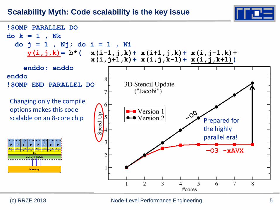
Scalability Myth: Code scalability is the key issue
(c) RRZE 2018 Node-Level Performance Engineering
Prepared for the highly parallel era!
!$OMP PARALLEL DO
do k = 1 , Nk
do j = 1 , Nj; do i = 1 , Ni
y(i,j,k)= b*( x(i-1,j,k)+ x(i+1,j,k)+ x(i,j-1,k)+ x(i,j+1,k)+ x(i,j,k-1)+ x(i,j,k+1))
enddo; enddo
enddo
!$OMP END PARALLEL DO
Changing only the compile options makes this code scalable on an 8-core chip
–O3 -xAVX
5
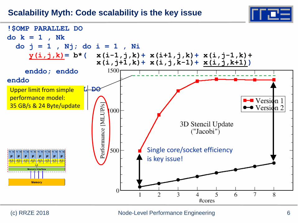
Scalability Myth: Code scalability is the key issue
(c) RRZE 2018 Node-Level Performance Engineering
!$OMP PARALLEL DO
do k = 1 , Nk
do j = 1 , Nj; do i = 1 , Ni
y(i,j,k)= b*( x(i-1,j,k)+ x(i+1,j,k)+ x(i,j-1,k)+ x(i,j+1,k)+ x(i,j,k-1)+ x(i,j,k+1))
enddo; enddo
enddo
!$OMP END PARALLEL DO
Single core/socket efficiency is key issue!
Upper limit from simple performance model:35 GB/s & 24 Byte/update
6
Questions to ask in high performance computing
Do I understand the performance behavior of my code?
Does the performance match a model I have made?
What is the optimal performance for my code on a given machine?
High Performance Computing == Computing at the bottleneck
Can I change my code so that the “optimal performance” gets
higher?
Circumventing/ameliorating the impact of the bottleneck
My model does not work – what’s wrong?
This is the good case, because you learn something
Performance monitoring / microbenchmarking may help clear up the
situation
(c) RRZE 2018 Node-Level Performance Engineering 7
Introduction:
Modern node architecture
A glance at basic core features:
pipelining, superscalarity, SMT, SIMD
Caches and data transfers through the memory hierarchy
Accelerators
Bottlenecks & hardware-software interaction
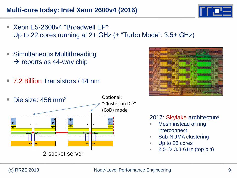
Multi-core today: Intel Xeon 2600v4 (2016)
Xeon E5-2600v4 “Broadwell EP”:
Up to 22 cores running at 2+ GHz (+ “Turbo Mode”: 3.5+ GHz)
Simultaneous Multithreading
reports as 44-way chip
7.2 Billion Transistors / 14 nm
Die size: 456 mm2
2-socket server
(c) RRZE 2018 Node-Level Performance Engineering
. . . . . .
Optional: “Cluster on Die” (CoD) mode
2017: Skylake architecture Mesh instead of ring
interconnect
Sub-NUMA clustering
Up to 28 cores
2.5 3.8 GHz (top bin)
9
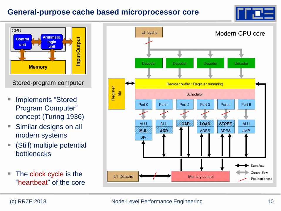
General-purpose cache based microprocessor core
Implements “Stored
Program Computer”
concept (Turing 1936)
Similar designs on all
modern systems
(Still) multiple potential
bottlenecks
The clock cycle is the
“heartbeat” of the core
(c) RRZE 2018 Node-Level Performance Engineering
Stored-program computer
Modern CPU core
10
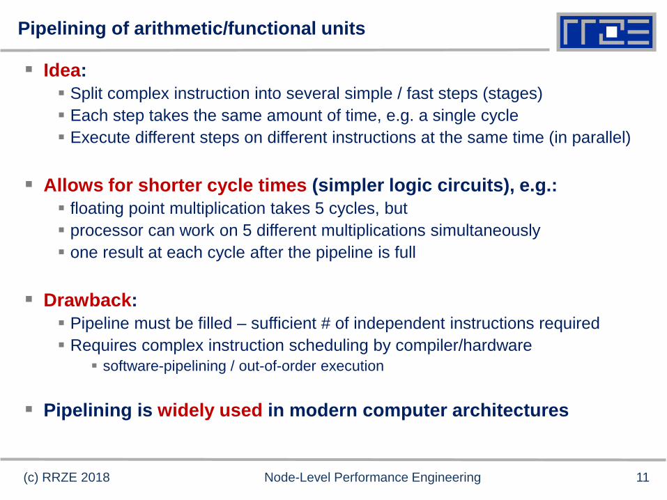
Pipelining of arithmetic/functional units
Idea:
Split complex instruction into several simple / fast steps (stages)
Each step takes the same amount of time, e.g. a single cycle
Execute different steps on different instructions at the same time (in parallel)
Allows for shorter cycle times (simpler logic circuits), e.g.:
floating point multiplication takes 5 cycles, but
processor can work on 5 different multiplications simultaneously
one result at each cycle after the pipeline is full
Drawback:
Pipeline must be filled – sufficient # of independent instructions required
Requires complex instruction scheduling by compiler/hardware
software-pipelining / out-of-order execution
Pipelining is widely used in modern computer architectures
(c) RRZE 2018 Node-Level Performance Engineering 11
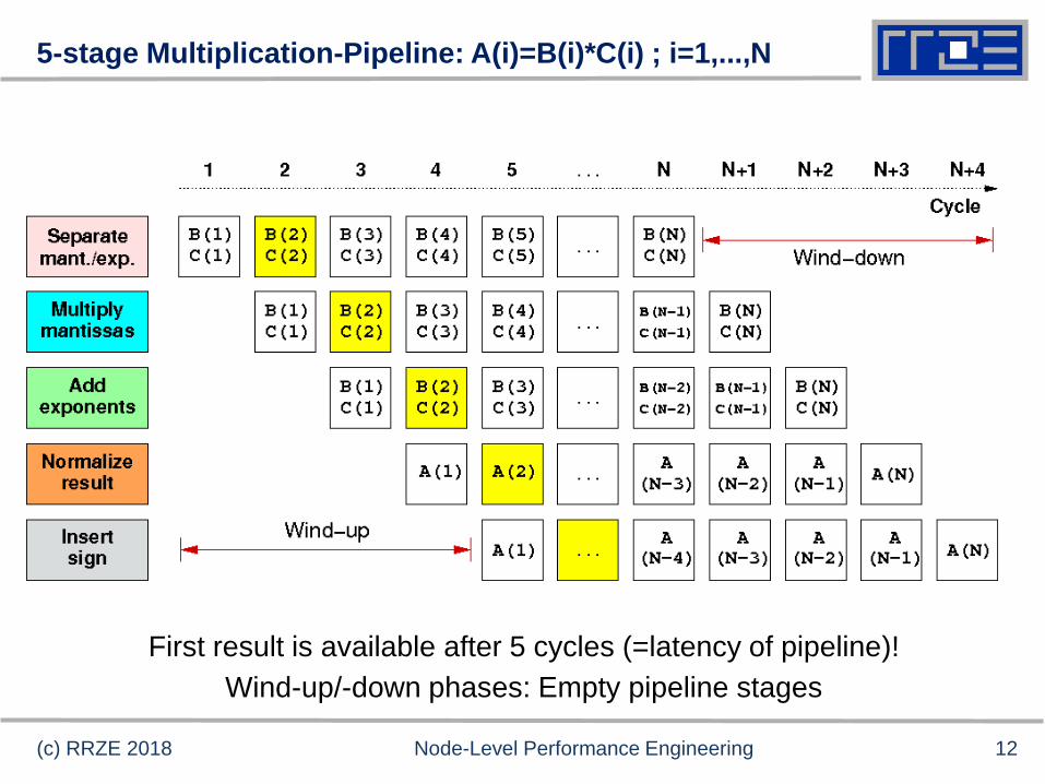
5-stage Multiplication-Pipeline: A(i)=B(i)*C(i) ; i=1,...,N
Wind-up/-down phases: Empty pipeline stages
First result is available after 5 cycles (=latency of pipeline)!
(c) RRZE 2018 Node-Level Performance Engineering 12
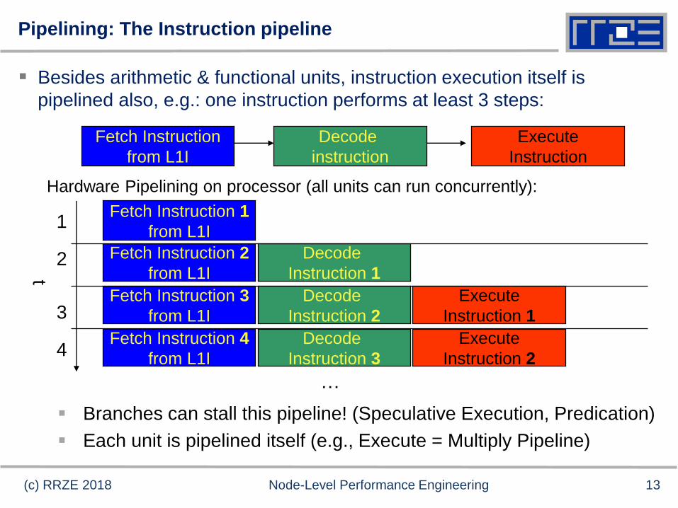
Pipelining: The Instruction pipeline
Besides arithmetic & functional units, instruction execution itself is
pipelined also, e.g.: one instruction performs at least 3 steps:
Fetch Instruction
from L1I
Decode
instruction
Execute
Instruction
Hardware Pipelining on processor (all units can run concurrently):
Fetch Instruction 1
from L1I
Decode
Instruction 1
Execute
Instruction 1
Fetch Instruction 2
from L1I
Decode
Instruction 2
Decode
Instruction 3
Execute
Instruction 2
Fetch Instruction 3
from L1I
Fetch Instruction 4
from L1I
t
…
Branches can stall this pipeline! (Speculative Execution, Predication)
Each unit is pipelined itself (e.g., Execute = Multiply Pipeline)
1
2
3
4
(c) RRZE 2018 Node-Level Performance Engineering 13
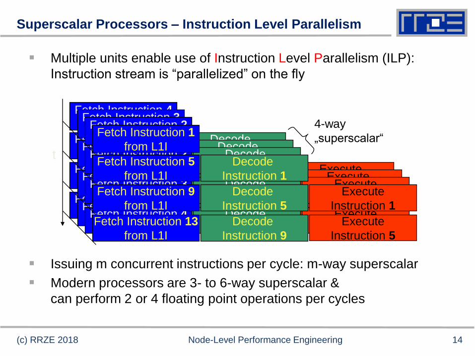
Multiple units enable use of Instruction Level Parallelism (ILP):
Instruction stream is “parallelized” on the fly
Issuing m concurrent instructions per cycle: m-way superscalar
Modern processors are 3- to 6-way superscalar &
can perform 2 or 4 floating point operations per cycles
Superscalar Processors – Instruction Level Parallelism
Fetch Instruction 4
from L1I
Decode
Instruction 1
Execute
Instruction 1
Fetch Instruction 2
from L1I
Decode
Instruction 2
Decode
Instruction 3
Execute
Instruction 2
Fetch Instruction 3
from L1I
Fetch Instruction 4
from L1I
Fetch Instruction 3
from L1I
Decode
Instruction 1
Execute
Instruction 1
Fetch Instruction 2
from L1I
Decode
Instruction 2
Decode
Instruction 3
Execute
Instruction 2
Fetch Instruction 3
from L1I
Fetch Instruction 4
from L1I
Fetch Instruction 2
from L1I
Decode
Instruction 1
Execute
Instruction 1
Fetch Instruction 2
from L1I
Decode
Instruction 2
Decode
Instruction 3
Execute
Instruction 2
Fetch Instruction 3
from L1I
Fetch Instruction 4
from L1I
Fetch Instruction 1
from L1I
Decode
Instruction 1
Execute
Instruction 1
Fetch Instruction 5
from L1I
Decode
Instruction 5
Decode
Instruction 9
Execute
Instruction 5
Fetch Instruction 9
from L1I
Fetch Instruction 13
from L1I
4-way
„superscalar“
t
(c) RRZE 2018 Node-Level Performance Engineering 14
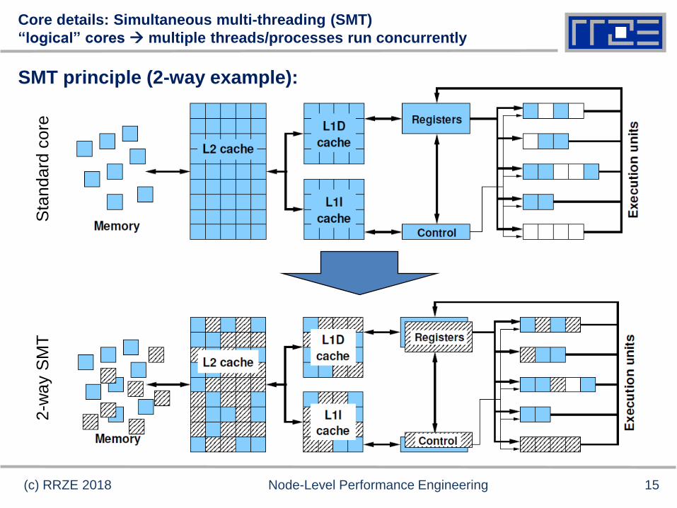
Core details: Simultaneous multi-threading (SMT)
“logical” cores multiple threads/processes run concurrently
(c) RRZE 2018 Node-Level Performance Engineering
Sta
ndard
core
2-w
ay S
MT
SMT principle (2-way example):
15
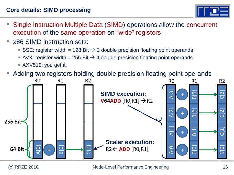
Core details: SIMD processing
Single Instruction Multiple Data (SIMD) operations allow the concurrent
execution of the same operation on “wide” registers
x86 SIMD instruction sets:
SSE: register width = 128 Bit 2 double precision floating point operands
AVX: register width = 256 Bit 4 double precision floating point operands
AXV512: you get it.
Adding two registers holding double precision floating point operands
(c) RRZE 2018 Node-Level Performance EngineeringA
[0]
A[1
]A
[2]
A[3
]
B[0
]B
[1]
B[2
]B
[3]
C[0
]C
[1]
C[2
]C
[3]
A[0
]
B[0
]
C[0
]
64 Bit
256 Bit
+ +
+
+
+
R0 R1 R2 R0 R1 R2
Scalar execution:
R2 ADD [R0,R1]
SIMD execution:
V64ADD [R0,R1] R2
16
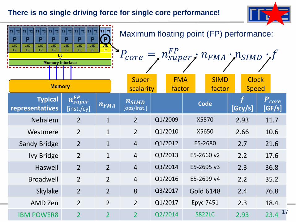
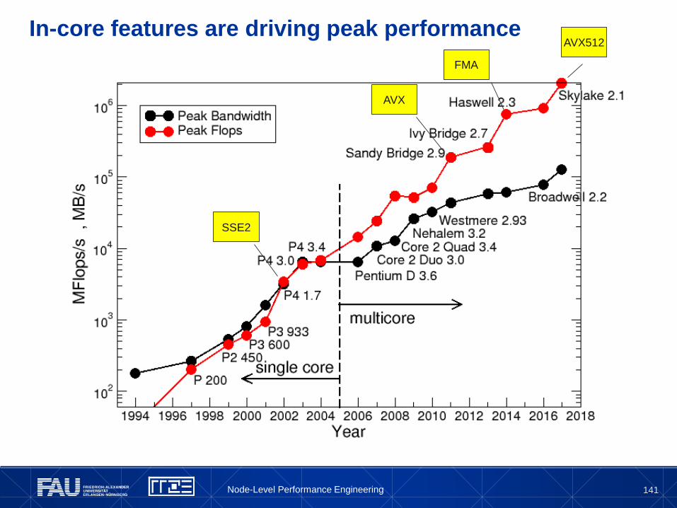
There is no single driving force for single core performance!
Maximum floating point (FP) performance:
𝑃𝑐𝑜𝑟𝑒 = 𝑛𝑠𝑢𝑝𝑒𝑟𝐹𝑃 ∙ 𝑛𝐹𝑀𝐴 ∙ 𝑛𝑆𝐼𝑀𝐷 ∙ 𝑓
(c) RRZE 2018 Node-Level Performance Engineering
Super-scalarity
FMAfactor
SIMDfactor
ClockSpeed
Typicalrepresentatives
𝒏𝒔𝒖𝒑𝒆𝒓𝑭𝑷
[inst./cy]𝒏𝑭𝑴𝑨
𝒏𝑺𝑰𝑴𝑫[ops/inst.]
Code𝒇
[Gcy/s]𝑷𝒄𝒐𝒓𝒆
[GF/s]
Nehalem 2 1 2 Q1/2009 X5570 2.93 11.7
Westmere 2 1 2 Q1/2010 X5650 2.66 10.6
Sandy Bridge 2 1 4 Q1/2012 E5-2680 2.7 21.6
Ivy Bridge 2 1 4 Q3/2013 E5-2660 v2 2.2 17.6
Haswell 2 2 4 Q3/2014 E5-2695 v3 2.3 36.8
Broadwell 2 2 4 Q1/2016 E5-2699 v4 2.2 35.2
Skylake 2 2 8 Q3/2017 Gold 6148 2.4 76.8
AMD Zen 2 2 2 Q1/2017 Epyc 7451 2.3 18.4
IBM POWER8 2 2 2 Q2/2014 S822LC 2.93 23.4 17
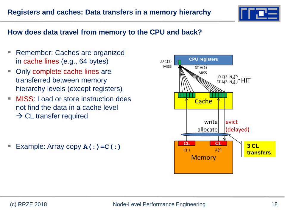
Registers and caches: Data transfers in a memory hierarchy
How does data travel from memory to the CPU and back?
Remember: Caches are organized
in cache lines (e.g., 64 bytes)
Only complete cache lines are
transferred between memory
hierarchy levels (except registers)
MISS: Load or store instruction does
not find the data in a cache level
CL transfer required
Example: Array copy A(:)=C(:)
(c) RRZE 2018 Node-Level Performance Engineering
CPU registers
Cache
Memory
CL
CL CL
CL
LD C(1)
MISS
ST A(1)MISS
writeallocate
evict(delayed)
3 CL
transfers
LD C(2..Ncl)ST A(2..Ncl) HIT
C(:) A(:)
18
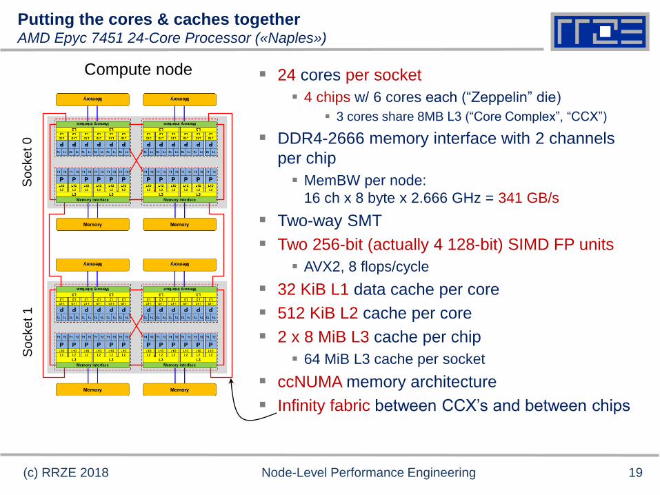
Putting the cores & caches togetherAMD Epyc 7451 24-Core Processor («Naples»)
(c) RRZE 2018 Node-Level Performance Engineering
So
cke
t 0
So
cke
t 1
24 cores per socket
4 chips w/ 6 cores each (“Zeppelin” die)
3 cores share 8MB L3 (“Core Complex”, “CCX”)
DDR4-2666 memory interface with 2 channels
per chip
MemBW per node:
16 ch x 8 byte x 2.666 GHz = 341 GB/s
Two-way SMT
Two 256-bit (actually 4 128-bit) SIMD FP units
AVX2, 8 flops/cycle
32 KiB L1 data cache per core
512 KiB L2 cache per core
2 x 8 MiB L3 cache per chip
64 MiB L3 cache per socket
ccNUMA memory architecture
Infinity fabric between CCX’s and between chips
Compute node
19
Interlude:
A glance at current accelerator technology
NVidia “Pascal” GP100
vs.
Intel Xeon Phi “Knights Landing”
21
NVidia Pascal GP100 block diagram
(c) RRZE 2018 Node-Level Performance Engineering
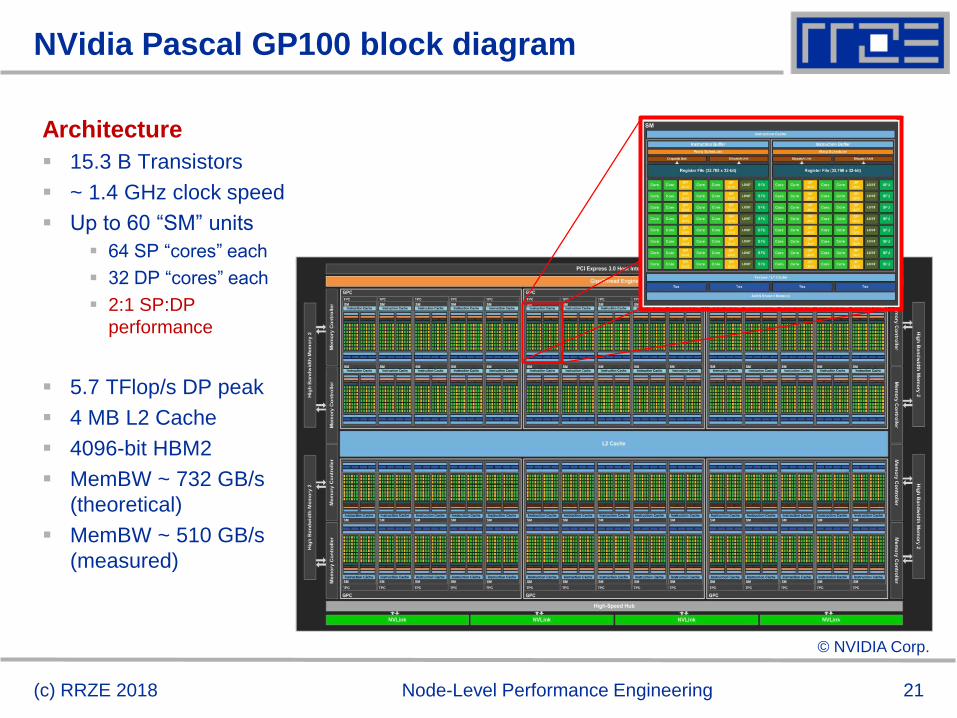
Architecture
15.3 B Transistors
~ 1.4 GHz clock speed
Up to 60 “SM” units
64 SP “cores” each
32 DP “cores” each
2:1 SP:DP
performance
5.7 TFlop/s DP peak
4 MB L2 Cache
4096-bit HBM2
MemBW ~ 732 GB/s
(theoretical)
MemBW ~ 510 GB/s
(measured)
© NVIDIA Corp.
22
Intel Xeon Phi “Knights Landing” block diagram
(c) RRZE 2018 Node-Level Performance Engineering
MCDRAM MCDRAM MCDRAM MCDRAM
MCDRAM MCDRAM MCDRAM MCDRAM
DDR4
DDR4
DDR4
DDR4
DDR4
DDR4
36 tiles
(72 cores)
max.
P P32 KiB L1 32 KiB L1
1 MiB L2
VPU
VPU
VPU
VPU
TTTT TTTT
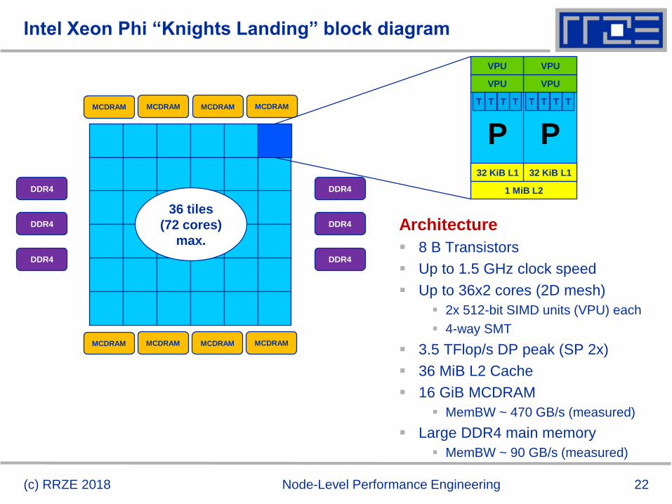
Architecture
8 B Transistors
Up to 1.5 GHz clock speed
Up to 36x2 cores (2D mesh)
2x 512-bit SIMD units (VPU) each
4-way SMT
3.5 TFlop/s DP peak (SP 2x)
36 MiB L2 Cache
16 GiB MCDRAM
MemBW ~ 470 GB/s (measured)
Large DDR4 main memory
MemBW ~ 90 GB/s (measured)
23
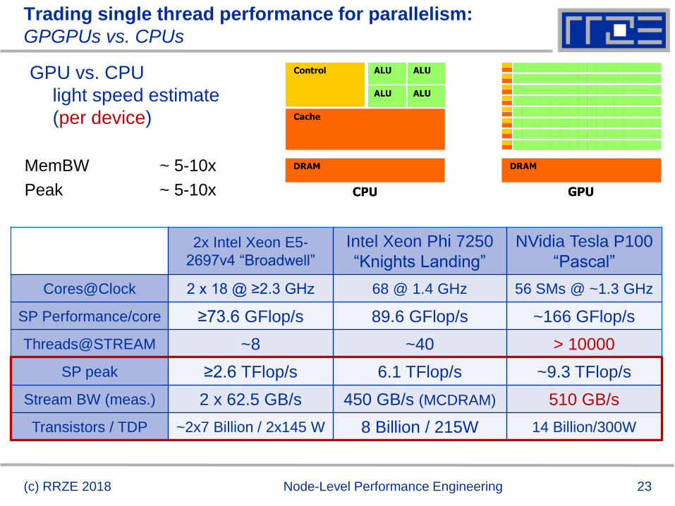
Trading single thread performance for parallelism:
GPGPUs vs. CPUs
GPU vs. CPU
light speed estimate
(per device)
MemBW ~ 5-10x
Peak ~ 5-10x
2x Intel Xeon E5-
2697v4 “Broadwell”
Intel Xeon Phi 7250
“Knights Landing”
NVidia Tesla P100
“Pascal”
Cores@Clock 2 x 18 @ ≥2.3 GHz 68 @ 1.4 GHz 56 SMs @ ~1.3 GHz
SP Performance/core ≥73.6 GFlop/s 89.6 GFlop/s ~166 GFlop/s
Threads@STREAM ~8 ~40 > 10000
SP peak ≥2.6 TFlop/s 6.1 TFlop/s ~9.3 TFlop/s
Stream BW (meas.) 2 x 62.5 GB/s 450 GB/s (MCDRAM) 510 GB/s
Transistors / TDP ~2x7 Billion / 2x145 W 8 Billion / 215W 14 Billion/300W
(c) RRZE 2018 Node-Level Performance Engineering
Node topology and
programming models
25
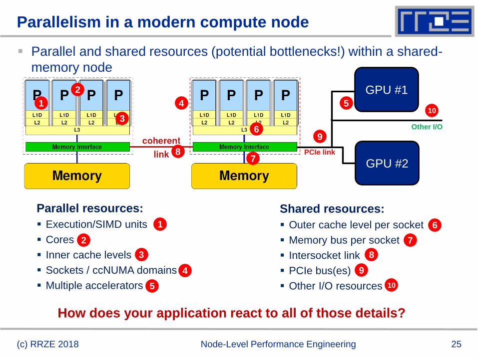
Parallelism in a modern compute node
Parallel and shared resources (potential bottlenecks!) within a shared-
memory node
GPU #1
GPU #2PCIe link
Parallel resources:
Execution/SIMD units
Cores
Inner cache levels
Sockets / ccNUMA domains
Multiple accelerators
Shared resources:
Outer cache level per socket
Memory bus per socket
Intersocket link
PCIe bus(es)
Other I/O resources
Other I/O
1
2
3
4 5
1
2
3
4
5
6
6
7
7
8
8
9
9
10
10
How does your application react to all of those details?
(c) RRZE 2018 Node-Level Performance Engineering
27(c) RRZE 2018 Node-Level Performance Engineering
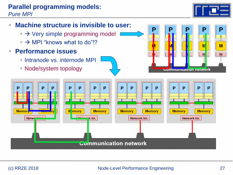
Parallel programming models:Pure MPI
Machine structure is invisible to user:
Very simple programming model
MPI “knows what to do”!?
Performance issues
Intranode vs. internode MPI
Node/system topology
28(c) RRZE 2018 Node-Level Performance Engineering
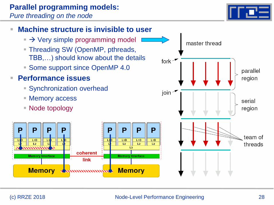
Parallel programming models:Pure threading on the node
Machine structure is invisible to user
Very simple programming model
Threading SW (OpenMP, pthreads,
TBB,…) should know about the details
Some support since OpenMP 4.0
Performance issues
Synchronization overhead
Memory access
Node topology
Conclusions about architecture
Modern computer architecture has a rich “topology”
Node-level hardware parallelism takes many forms
Sockets/devices – CPU: 1-8, GPGPU: 1-6
Cores – moderate (CPU: 4-16) to massive (GPGPU: 1000’s)
SIMD – moderate (CPU: 2-8) to massive (GPGPU: 10’s-100’s)
Superscalarity (CPU: 2-6)
Exploiting performance: parallelism + bottleneck awareness
“High Performance Computing” == computing at a bottleneck
Performance of programming models is sensitive to architecture
Topology/affinity influences overheads
Standards do not contain (many) topology-aware features
Apart from overheads, performance features are largely independent of the programming model
(c) RRZE 2018 Node-Level Performance Engineering 30
Multicore Performance and Tools
32
Tools for Node-level Performance Engineering
Gather Node Information
hwloc, likwid-topology, likwid-powermeter
Affinity control and data placement
OpenMP and MPI runtime environments, hwloc, numactl, likwid-pin
Runtime Profiling
Compilers, gprof, HPC Toolkit, …
Performance Profilers
Intel VtuneTM, likwid-perfctr, PAPI based tools, Linux perf, …
Microbenchmarking
STREAM, likwid-bench, lmbench
(c) RRZE 2018 Node-Level Performance Engineering
LIKWID performance tools
LIKWID tool suite:
Like
I
Knew
What
I’m
Doing
Open source tool collection
(developed at RRZE):
https://github.com/RRZE-HPC/likwid
J. Treibig, G. Hager, G. Wellein: LIKWID: A lightweight performance-oriented tool suite for x86 multicore environments. PSTI2010, Sep 13-16, 2010, San Diego, CA http://arxiv.org/abs/1004.4431
(c) RRZE 2018 Node-Level Performance Engineering 33
35(c) RRZE 2018 Node-Level Performance Engineering
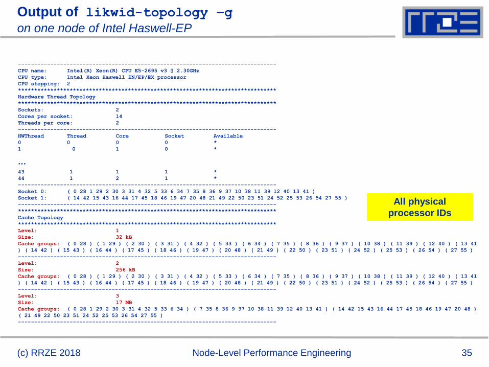
Output of likwid-topology –gon one node of Intel Haswell-EP
--------------------------------------------------------------------------------
CPU name: Intel(R) Xeon(R) CPU E5-2695 v3 @ 2.30GHz
CPU type: Intel Xeon Haswell EN/EP/EX processor
CPU stepping: 2
********************************************************************************
Hardware Thread Topology
********************************************************************************
Sockets: 2
Cores per socket: 14
Threads per core: 2
--------------------------------------------------------------------------------
HWThread Thread Core Socket Available
0 0 0 0 *
1 0 1 0 *
…43 1 1 1 *
44 1 2 1 *
--------------------------------------------------------------------------------
Socket 0: ( 0 28 1 29 2 30 3 31 4 32 5 33 6 34 7 35 8 36 9 37 10 38 11 39 12 40 13 41 )
Socket 1: ( 14 42 15 43 16 44 17 45 18 46 19 47 20 48 21 49 22 50 23 51 24 52 25 53 26 54 27 55 )
--------------------------------------------------------------------------------
********************************************************************************
Cache Topology
********************************************************************************
Level: 1
Size: 32 kB
Cache groups: ( 0 28 ) ( 1 29 ) ( 2 30 ) ( 3 31 ) ( 4 32 ) ( 5 33 ) ( 6 34 ) ( 7 35 ) ( 8 36 ) ( 9 37 ) ( 10 38 ) ( 11 39 ) ( 12 40 ) ( 13 41
) ( 14 42 ) ( 15 43 ) ( 16 44 ) ( 17 45 ) ( 18 46 ) ( 19 47 ) ( 20 48 ) ( 21 49 ) ( 22 50 ) ( 23 51 ) ( 24 52 ) ( 25 53 ) ( 26 54 ) ( 27 55 )
--------------------------------------------------------------------------------
Level: 2
Size: 256 kB
Cache groups: ( 0 28 ) ( 1 29 ) ( 2 30 ) ( 3 31 ) ( 4 32 ) ( 5 33 ) ( 6 34 ) ( 7 35 ) ( 8 36 ) ( 9 37 ) ( 10 38 ) ( 11 39 ) ( 12 40 ) ( 13 41
) ( 14 42 ) ( 15 43 ) ( 16 44 ) ( 17 45 ) ( 18 46 ) ( 19 47 ) ( 20 48 ) ( 21 49 ) ( 22 50 ) ( 23 51 ) ( 24 52 ) ( 25 53 ) ( 26 54 ) ( 27 55 )
--------------------------------------------------------------------------------
Level: 3
Size: 17 MB
Cache groups: ( 0 28 1 29 2 30 3 31 4 32 5 33 6 34 ) ( 7 35 8 36 9 37 10 38 11 39 12 40 13 41 ) ( 14 42 15 43 16 44 17 45 18 46 19 47 20 48 )
( 21 49 22 50 23 51 24 52 25 53 26 54 27 55 )
--------------------------------------------------------------------------------
All physical
processor IDs
36
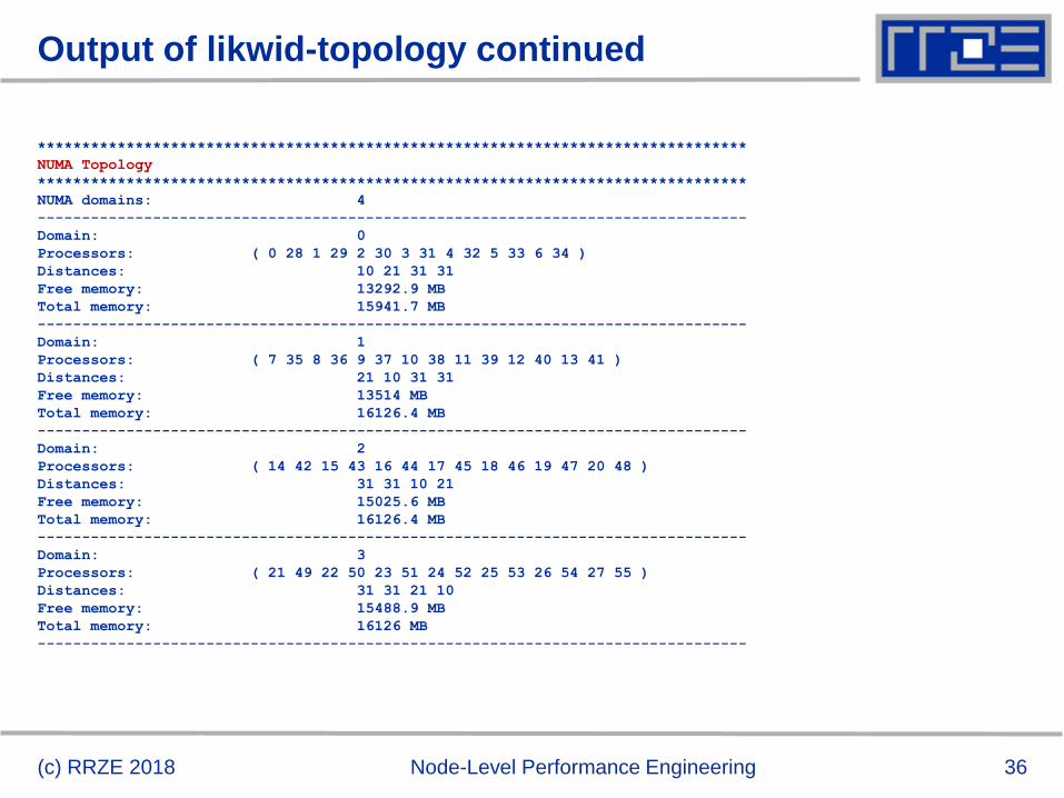
Output of likwid-topology continued
(c) RRZE 2018 Node-Level Performance Engineering
********************************************************************************
NUMA Topology
********************************************************************************
NUMA domains: 4
--------------------------------------------------------------------------------
Domain: 0
Processors: ( 0 28 1 29 2 30 3 31 4 32 5 33 6 34 )
Distances: 10 21 31 31
Free memory: 13292.9 MB
Total memory: 15941.7 MB
--------------------------------------------------------------------------------
Domain: 1
Processors: ( 7 35 8 36 9 37 10 38 11 39 12 40 13 41 )
Distances: 21 10 31 31
Free memory: 13514 MB
Total memory: 16126.4 MB
--------------------------------------------------------------------------------
Domain: 2
Processors: ( 14 42 15 43 16 44 17 45 18 46 19 47 20 48 )
Distances: 31 31 10 21
Free memory: 15025.6 MB
Total memory: 16126.4 MB
--------------------------------------------------------------------------------
Domain: 3
Processors: ( 21 49 22 50 23 51 24 52 25 53 26 54 27 55 )
Distances: 31 31 21 10
Free memory: 15488.9 MB
Total memory: 16126 MB
--------------------------------------------------------------------------------
37
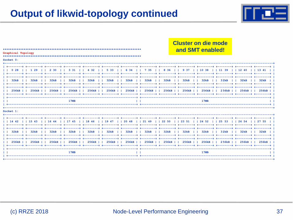
Output of likwid-topology continued
(c) RRZE 2018 Node-Level Performance Engineering
********************************************************************************
Graphical Topology
********************************************************************************
Socket 0:
+-----------------------------------------------------------------------------------------------------------------------------------------------------------+
| +--------+ +--------+ +--------+ +--------+ +--------+ +--------+ +--------+ +--------+ +--------+ +--------+ +--------+ +--------+ +--------+ +--------+ |
| | 0 28 | | 1 29 | | 2 30 | | 3 31 | | 4 32 | | 5 33 | | 6 34 | | 7 35 | | 8 36 | | 9 37 | | 10 38 | | 11 39 | | 12 40 | | 13 41 | |
| +--------+ +--------+ +--------+ +--------+ +--------+ +--------+ +--------+ +--------+ +--------+ +--------+ +--------+ +--------+ +--------+ +--------+ |
| +--------+ +--------+ +--------+ +--------+ +--------+ +--------+ +--------+ +--------+ +--------+ +--------+ +--------+ +--------+ +--------+ +--------+ |
| | 32kB | | 32kB | | 32kB | | 32kB | | 32kB | | 32kB | | 32kB | | 32kB | | 32kB | | 32kB | | 32kB | | 32kB | | 32kB | | 32kB | |
| +--------+ +--------+ +--------+ +--------+ +--------+ +--------+ +--------+ +--------+ +--------+ +--------+ +--------+ +--------+ +--------+ +--------+ |
| +--------+ +--------+ +--------+ +--------+ +--------+ +--------+ +--------+ +--------+ +--------+ +--------+ +--------+ +--------+ +--------+ +--------+ |
| | 256kB | | 256kB | | 256kB | | 256kB | | 256kB | | 256kB | | 256kB | | 256kB | | 256kB | | 256kB | | 256kB | | 256kB | | 256kB | | 256kB | |
| +--------+ +--------+ +--------+ +--------+ +--------+ +--------+ +--------+ +--------+ +--------+ +--------+ +--------+ +--------+ +--------+ +--------+ |
| +--------------------------------------------------------------------------+ +--------------------------------------------------------------------------+ |
| | 17MB | | 17MB | |
| +--------------------------------------------------------------------------+ +--------------------------------------------------------------------------+ |
+-----------------------------------------------------------------------------------------------------------------------------------------------------------+
Socket 1:
+-----------------------------------------------------------------------------------------------------------------------------------------------------------+
| +--------+ +--------+ +--------+ +--------+ +--------+ +--------+ +--------+ +--------+ +--------+ +--------+ +--------+ +--------+ +--------+ +--------+ |
| | 14 42 | | 15 43 | | 16 44 | | 17 45 | | 18 46 | | 19 47 | | 20 48 | | 21 49 | | 22 50 | | 23 51 | | 24 52 | | 25 53 | | 26 54 | | 27 55 | |
| +--------+ +--------+ +--------+ +--------+ +--------+ +--------+ +--------+ +--------+ +--------+ +--------+ +--------+ +--------+ +--------+ +--------+ |
| +--------+ +--------+ +--------+ +--------+ +--------+ +--------+ +--------+ +--------+ +--------+ +--------+ +--------+ +--------+ +--------+ +--------+ |
| | 32kB | | 32kB | | 32kB | | 32kB | | 32kB | | 32kB | | 32kB | | 32kB | | 32kB | | 32kB | | 32kB | | 32kB | | 32kB | | 32kB | |
| +--------+ +--------+ +--------+ +--------+ +--------+ +--------+ +--------+ +--------+ +--------+ +--------+ +--------+ +--------+ +--------+ +--------+ |
| +--------+ +--------+ +--------+ +--------+ +--------+ +--------+ +--------+ +--------+ +--------+ +--------+ +--------+ +--------+ +--------+ +--------+ |
| | 256kB | | 256kB | | 256kB | | 256kB | | 256kB | | 256kB | | 256kB | | 256kB | | 256kB | | 256kB | | 256kB | | 256kB | | 256kB | | 256kB | |
| +--------+ +--------+ +--------+ +--------+ +--------+ +--------+ +--------+ +--------+ +--------+ +--------+ +--------+ +--------+ +--------+ +--------+ |
| +--------------------------------------------------------------------------+ +--------------------------------------------------------------------------+ |
| | 17MB | | 17MB | |
| +--------------------------------------------------------------------------+ +--------------------------------------------------------------------------+ |
+-----------------------------------------------------------------------------------------------------------------------------------------------------------+
Cluster on die mode
and SMT enabled!
Enforcing thread/process-core affinity
under the Linux OS
Standard tools and OS affinity facilities under
program control
likwid-pin
39(c) RRZE 2018 Node-Level Performance Engineering
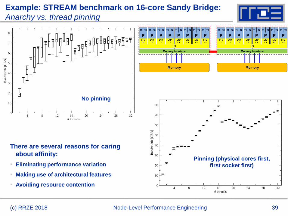
Example: STREAM benchmark on 16-core Sandy Bridge:
Anarchy vs. thread pinning
No pinning
Pinning (physical cores first,
first socket first)
There are several reasons for caring
about affinity:
Eliminating performance variation
Making use of architectural features
Avoiding resource contention
41(c) RRZE 2018 Node-Level Performance Engineering
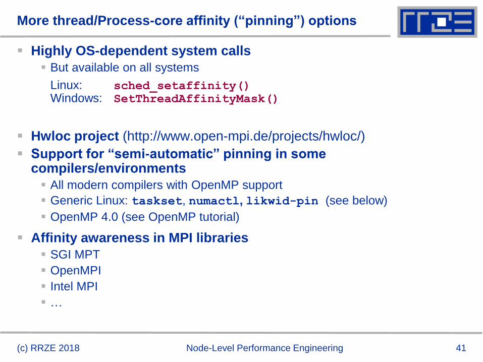
More thread/Process-core affinity (“pinning”) options
Highly OS-dependent system calls
But available on all systems
Linux: sched_setaffinity()
Windows: SetThreadAffinityMask()
Hwloc project (http://www.open-mpi.de/projects/hwloc/)
Support for “semi-automatic” pinning in some compilers/environments
All modern compilers with OpenMP support
Generic Linux: taskset, numactl, likwid-pin (see below)
OpenMP 4.0 (see OpenMP tutorial)
Affinity awareness in MPI libraries
SGI MPT
OpenMPI
Intel MPI
…
42(c) RRZE 2018 Node-Level Performance Engineering
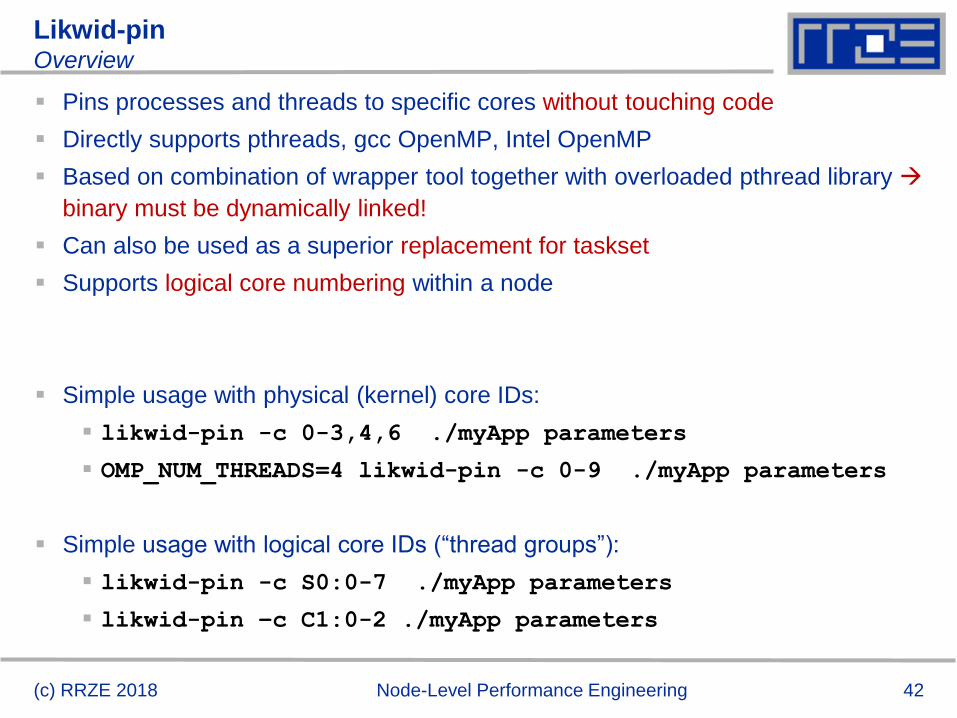
Likwid-pinOverview
Pins processes and threads to specific cores without touching code
Directly supports pthreads, gcc OpenMP, Intel OpenMP
Based on combination of wrapper tool together with overloaded pthread library
binary must be dynamically linked!
Can also be used as a superior replacement for taskset
Supports logical core numbering within a node
Simple usage with physical (kernel) core IDs:
likwid-pin -c 0-3,4,6 ./myApp parameters
OMP_NUM_THREADS=4 likwid-pin -c 0-9 ./myApp parameters
Simple usage with logical core IDs (“thread groups”):
likwid-pin -c S0:0-7 ./myApp parameters
likwid-pin –c C1:0-2 ./myApp parameters
43(c) RRZE 2018 Node-Level Performance Engineering
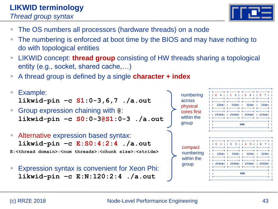
LIKWID terminologyThread group syntax
The OS numbers all processors (hardware threads) on a node
The numbering is enforced at boot time by the BIOS and may have nothing to
do with topological entities
LIKWID concept: thread group consisting of HW threads sharing a topological
entity (e.g., socket, shared cache,…)
A thread group is defined by a single character + index
Example:likwid-pin –c S1:0-3,6,7 ./a.out
Group expression chaining with @:
likwid-pin –c S0:0-3@S1:0-3 ./a.out
Alternative expression based syntax:likwid-pin –c E:S0:4:2:4 ./a.out
E:<thread domain>:<num threads>:<chunk size>:<stride>
Expression syntax is convenient for Xeon Phi: likwid-pin –c E:N:120:2:4 ./a.out
+-------------------------------------+
| +------+ +------+ +------+ +------+ |
| | 0 4 | | 1 5 | | 2 6 | | 3 7 | |
| +------+ +------+ +------+ +------+ |
| +------+ +------+ +------+ +------+ |
| | 32kB| | 32kB| | 32kB| | 32kB| |
| +------+ +------+ +------+ +------+ |
| +------+ +------+ +------+ +------+ |
| | 256kB| | 256kB| | 256kB| | 256kB| |
| +------+ +------+ +------+ +------+ |
| +---------------------------------+ |
| | 8MB | |
| +---------------------------------+ |
+-------------------------------------+
numbering
across
physical
cores first
within the
group
+-------------------------------------+
| +------+ +------+ +------+ +------+ |
| | 0 1 | | 2 3 | | 4 5 | | 6 7 | |
| +------+ +------+ +------+ +------+ |
| +------+ +------+ +------+ +------+ |
| | 32kB| | 32kB| | 32kB| | 32kB| |
| +------+ +------+ +------+ +------+ |
| +------+ +------+ +------+ +------+ |
| | 256kB| | 256kB| | 256kB| | 256kB| |
| +------+ +------+ +------+ +------+ |
| +---------------------------------+ |
| | 8MB | |
| +---------------------------------+ |
+-------------------------------------+
compact
numbering
within the
group
44
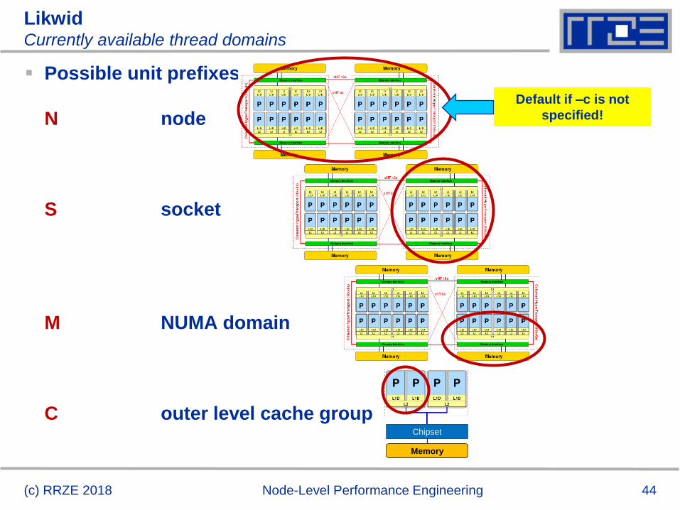
LikwidCurrently available thread domains
Possible unit prefixes
N node
S socket
M NUMA domain
C outer level cache group
(c) RRZE 2018 Node-Level Performance Engineering
Chipset
Memory
Default if –c is not
specified!

45(c) RRZE 2018 Node-Level Performance Engineering
Likwid-pinExample: Intel OpenMP
Running the STREAM benchmark with likwid-pin:
$ likwid-pin -c S0:0-3 ./stream
----------------------------------------------
Double precision appears to have 16 digits of accuracy
Assuming 8 bytes per DOUBLE PRECISION word
----------------------------------------------
Array size = 20000000
Offset = 32
The total memory requirement is 457 MB
You are running each test 10 times
--
The *best* time for each test is used
*EXCLUDING* the first and last iterations
[pthread wrapper] MAIN -> 0
[pthread wrapper] PIN_MASK: 0->1 1->2 2->3
[pthread wrapper] SKIP MASK: 0x1
threadid 140668624234240 -> SKIP
threadid 140668598843264 -> core 1 - OK
threadid 140668594644992 -> core 2 - OK
threadid 140668590446720 -> core 3 - OK
[... rest of STREAM output omitted ...]
Skip shepherd
thread if necessary
Main PID always
pinned
Pin all spawned
threads in turn
Clock speed under the Linux OS
likwid-powermeter
likwid-setFrequencies
47
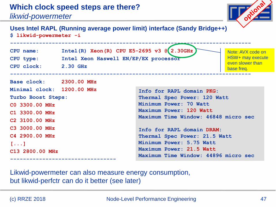
Which clock speed steps are there?
likwid-powermeter
Uses Intel RAPL (Running average power limit) interface (Sandy Bridge++)$ likwid-powermeter -i
---------------------------------------------------------------------------
CPU name: Intel(R) Xeon(R) CPU E5-2695 v3 @ 2.30GHz
CPU type: Intel Xeon Haswell EN/EP/EX processor
CPU clock: 2.30 GHz
---------------------------------------------------------------------------
Base clock: 2300.00 MHz
Minimal clock: 1200.00 MHz
Turbo Boost Steps:
C0 3300.00 MHz
C1 3300.00 MHz
C2 3100.00 MHz
C3 3000.00 MHz
C4 2900.00 MHz
[...]
C13 2800.00 MHz
---------------------------------
(c) RRZE 2018 Node-Level Performance Engineering
Info for RAPL domain PKG:
Thermal Spec Power: 120 Watt
Minimum Power: 70 Watt
Maximum Power: 120 Watt
Maximum Time Window: 46848 micro sec
Info for RAPL domain DRAM:
Thermal Spec Power: 21.5 Watt
Minimum Power: 5.75 Watt
Maximum Power: 21.5 Watt
Maximum Time Window: 44896 micro sec
Likwid-powermeter can also measure energy consumption,
but likwid-perfctr can do it better (see later)
Note: AVX code on
HSW+ may execute
even slower than
base freq.
48
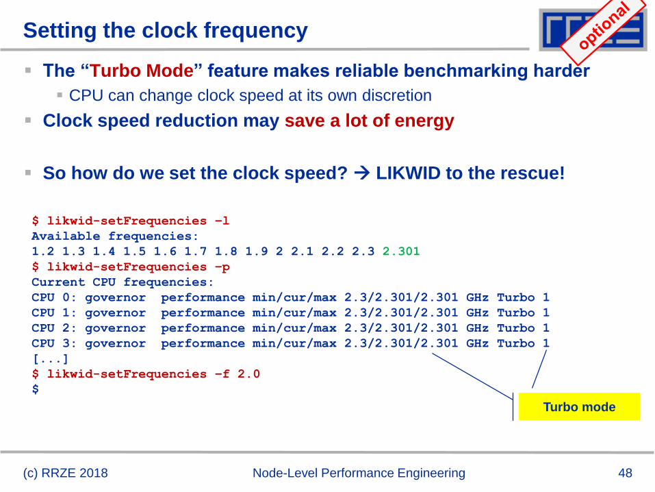
Setting the clock frequency
The “Turbo Mode” feature makes reliable benchmarking harder
CPU can change clock speed at its own discretion
Clock speed reduction may save a lot of energy
So how do we set the clock speed? LIKWID to the rescue!
(c) RRZE 2018 Node-Level Performance Engineering
$ likwid-setFrequencies –l
Available frequencies:
1.2 1.3 1.4 1.5 1.6 1.7 1.8 1.9 2 2.1 2.2 2.3 2.301
$ likwid-setFrequencies –p
Current CPU frequencies:
CPU 0: governor performance min/cur/max 2.3/2.301/2.301 GHz Turbo 1
CPU 1: governor performance min/cur/max 2.3/2.301/2.301 GHz Turbo 1
CPU 2: governor performance min/cur/max 2.3/2.301/2.301 GHz Turbo 1
CPU 3: governor performance min/cur/max 2.3/2.301/2.301 GHz Turbo 1
[...]
$ likwid-setFrequencies –f 2.0
$
Turbo mode
49
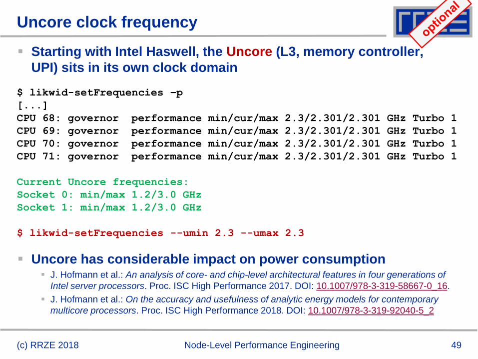
Uncore clock frequency
Starting with Intel Haswell, the Uncore (L3, memory controller,
UPI) sits in its own clock domain
Uncore has considerable impact on power consumption J. Hofmann et al.: An analysis of core- and chip-level architectural features in four generations of
Intel server processors. Proc. ISC High Performance 2017. DOI: 10.1007/978-3-319-58667-0_16.
J. Hofmann et al.: On the accuracy and usefulness of analytic energy models for contemporary
multicore processors. Proc. ISC High Performance 2018. DOI: 10.1007/978-3-319-92040-5_2
(c) RRZE 2018 Node-Level Performance Engineering
$ likwid-setFrequencies –p
[...]
CPU 68: governor performance min/cur/max 2.3/2.301/2.301 GHz Turbo 1
CPU 69: governor performance min/cur/max 2.3/2.301/2.301 GHz Turbo 1
CPU 70: governor performance min/cur/max 2.3/2.301/2.301 GHz Turbo 1
CPU 71: governor performance min/cur/max 2.3/2.301/2.301 GHz Turbo 1
Current Uncore frequencies:
Socket 0: min/max 1.2/3.0 GHz
Socket 1: min/max 1.2/3.0 GHz
$ likwid-setFrequencies --umin 2.3 --umax 2.3
50
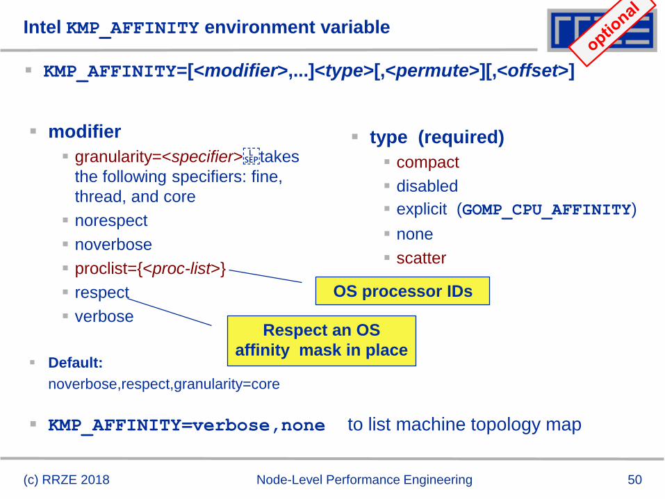
Intel KMP_AFFINITY environment variable
KMP_AFFINITY=[<modifier>,...]<type>[,<permute>][,<offset>]
modifier
granularity=<specifier>takes
the following specifiers: fine,
thread, and core
norespect
noverbose
proclist={<proc-list>}
respect
verbose
Default:
noverbose,respect,granularity=core
type (required)
compact
disabled
explicit (GOMP_CPU_AFFINITY)
none
scatter
KMP_AFFINITY=verbose,none to list machine topology map
OS processor IDs
Respect an OS
affinity mask in place
(c) RRZE 2018 Node-Level Performance Engineering
51
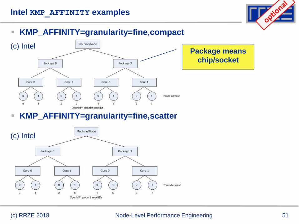
Intel KMP_AFFINITY examples
KMP_AFFINITY=granularity=fine,compact
KMP_AFFINITY=granularity=fine,scatter
Package means
chip/socket
(c) Intel
(c) Intel
(c) RRZE 2018 Node-Level Performance Engineering
52
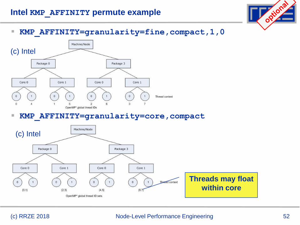
Intel KMP_AFFINITY permute example
KMP_AFFINITY=granularity=fine,compact,1,0
KMP_AFFINITY=granularity=core,compact
(c) Intel
(c) Intel
Threads may float
within core
(c) RRZE 2018 Node-Level Performance Engineering
53
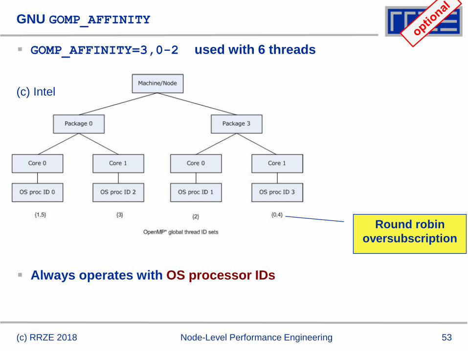
GNU GOMP_AFFINITY
GOMP_AFFINITY=3,0-2 used with 6 threads
Always operates with OS processor IDs
Round robin
oversubscription
(c) Intel
(c) RRZE 2018 Node-Level Performance Engineering
Microbenchmarking for
architectural exploration (and more)
Probing of the memory hierarchy
Saturation effects in cache and memory
55
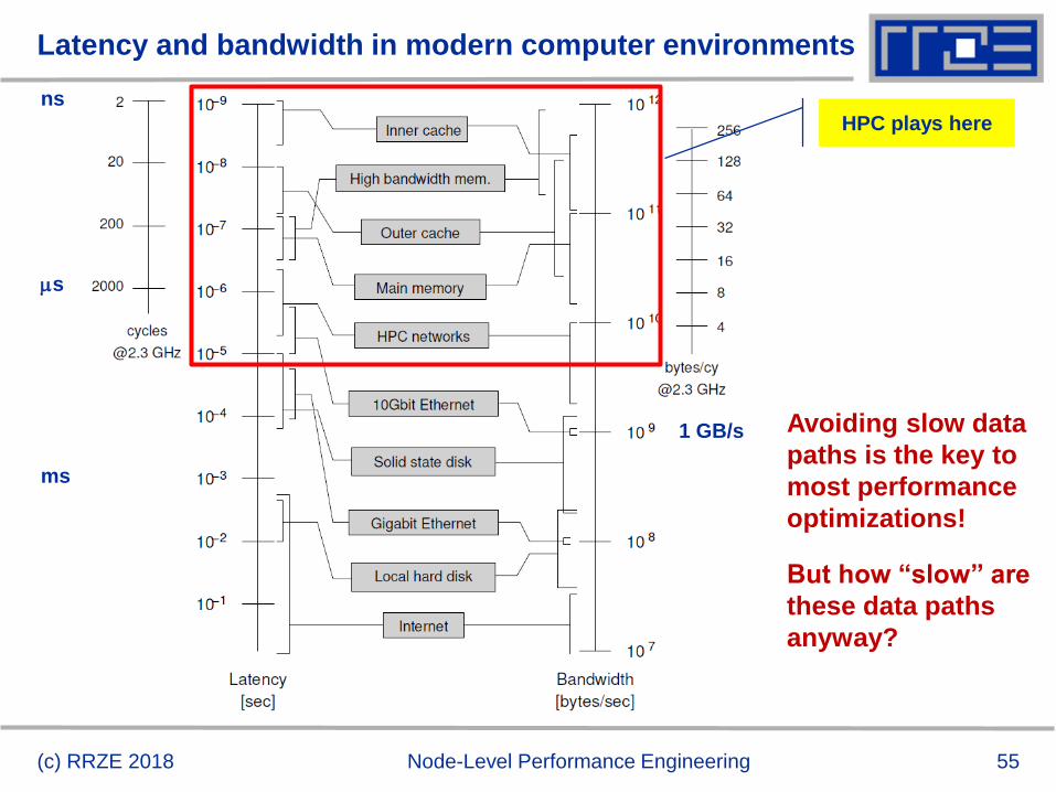
Latency and bandwidth in modern computer environments
ns
ms
ms
1 GB/s
(c) RRZE 2018 Node-Level Performance Engineering
HPC plays here
Avoiding slow data
paths is the key to
most performance
optimizations!
But how “slow” are
these data paths
anyway?
56
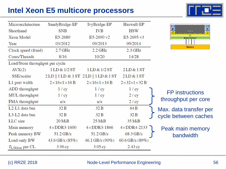
Intel Xeon E5 multicore processors
(c) RRZE 2018 Node-Level Performance Engineering
FP instructions
throughput per core
Max. data transfer per
cycle between caches
Peak main memory
bandwidth
…
57(c) RRZE 2018 Node-Level Performance Engineering
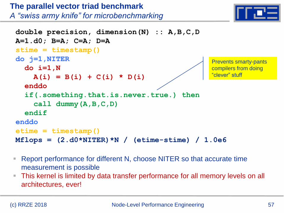
The parallel vector triad benchmark
A “swiss army knife” for microbenchmarking
Report performance for different N, choose NITER so that accurate time
measurement is possible
This kernel is limited by data transfer performance for all memory levels on all
architectures, ever!
double precision, dimension(N) :: A,B,C,D
A=1.d0; B=A; C=A; D=A
stime = timestamp()
do j=1,NITER
do i=1,N
A(i) = B(i) + C(i) * D(i)
enddo
if(.something.that.is.never.true.) then
call dummy(A,B,C,D)
endif
enddo
etime = timestamp()
Mflops = (2.d0*NITER)*N / (etime-stime) / 1.0e6
Prevents smarty-pants
compilers from doing
“clever” stuff
58
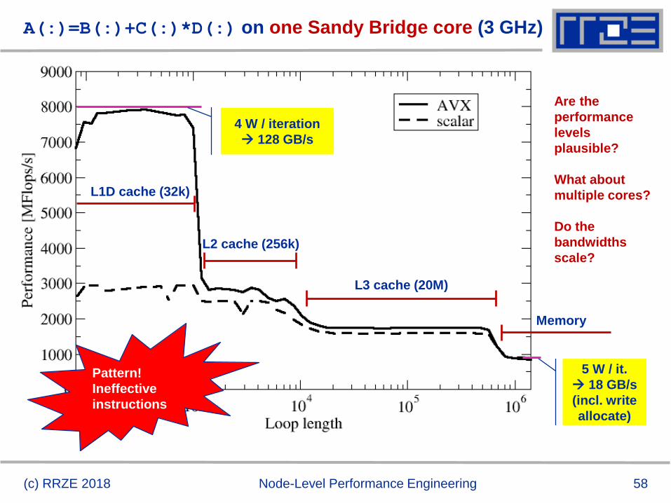
A(:)=B(:)+C(:)*D(:) on one Sandy Bridge core (3 GHz)
(c) RRZE 2018 Node-Level Performance Engineering
L1D cache (32k)
L2 cache (256k)
L3 cache (20M)
Memory
4 W / iteration
128 GB/s
5 W / it.
18 GB/s
(incl. write
allocate)
Are the
performance
levels
plausible?
What about
multiple cores?
Do the
bandwidths
scale?
Pattern!
Ineffective
instructions
59
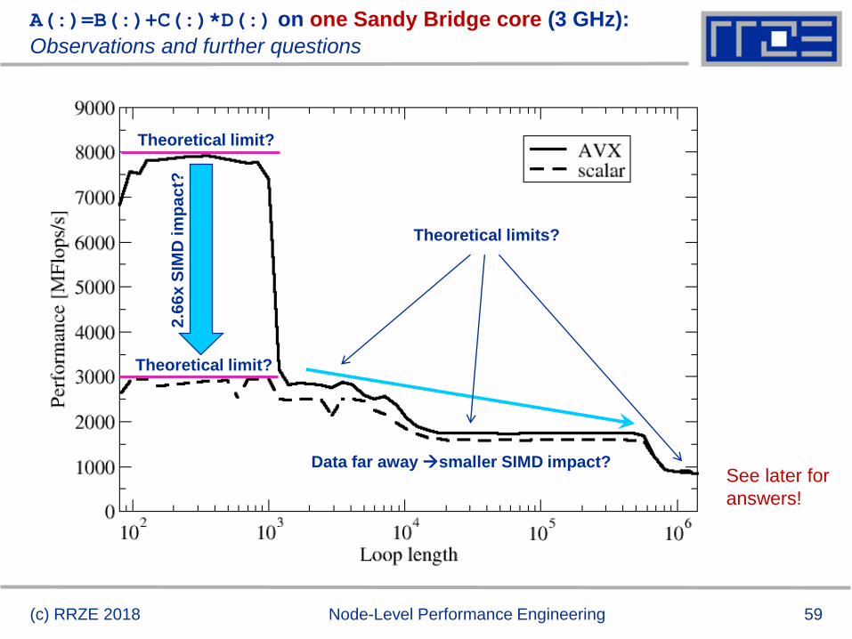
A(:)=B(:)+C(:)*D(:) on one Sandy Bridge core (3 GHz):
Observations and further questions
(c) RRZE 2018 Node-Level Performance Engineering
2.6
6x
SIM
D im
pa
ct?
Data far awaysmaller SIMD impact?
Theoretical limit?
Theoretical limit?
Theoretical limits?
See later for
answers!
60
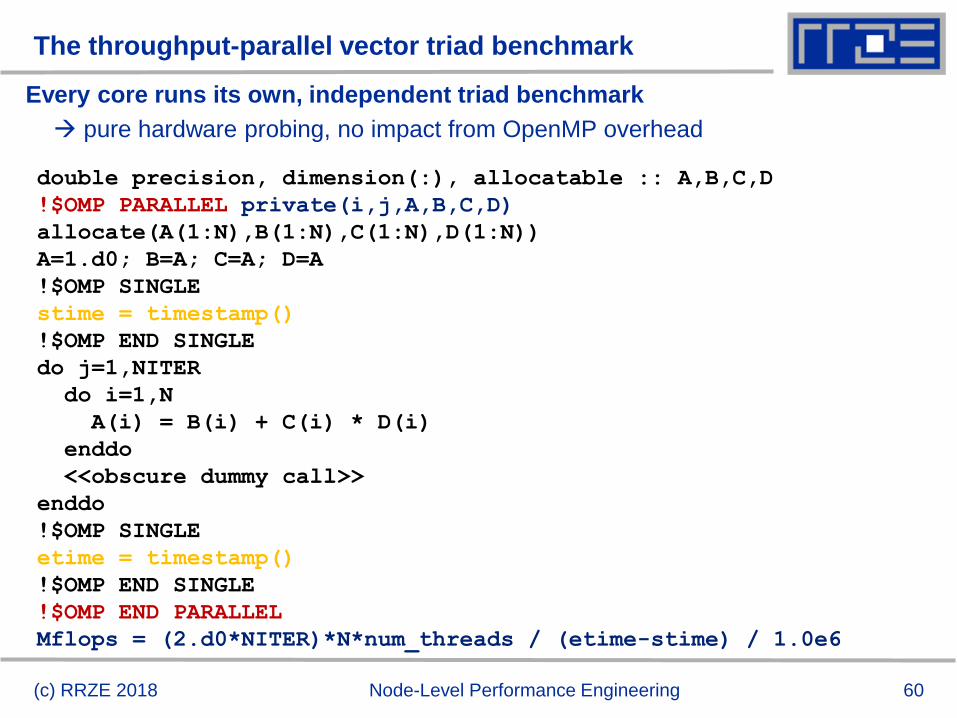
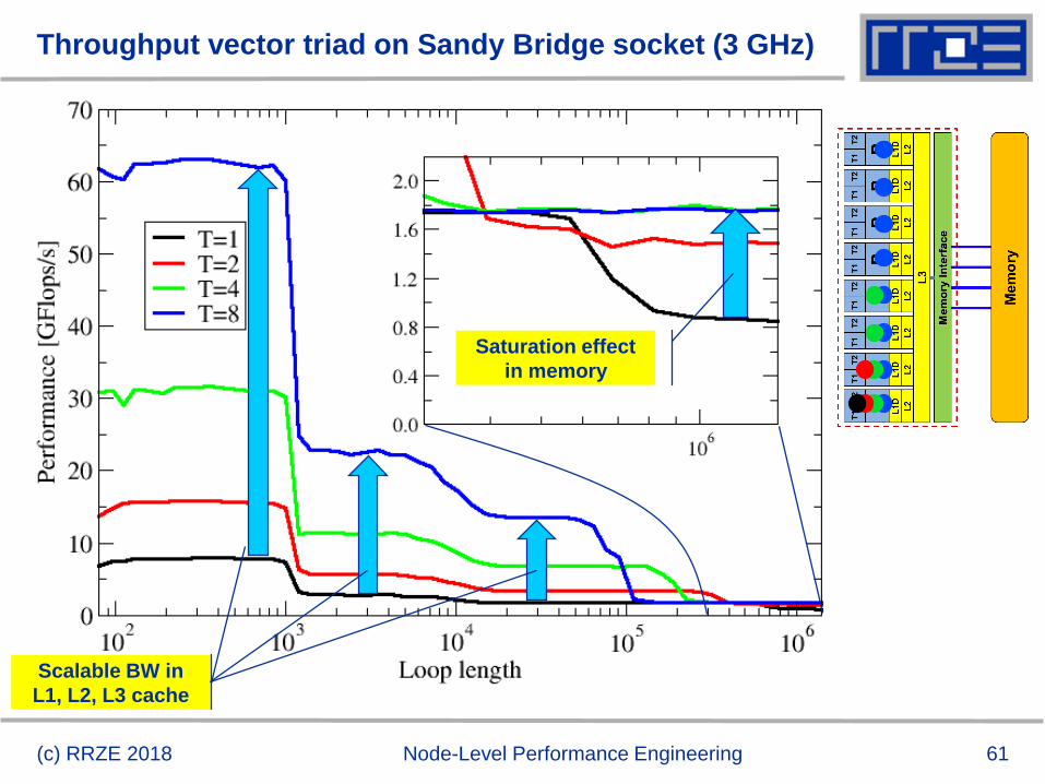
The throughput-parallel vector triad benchmark
Every core runs its own, independent triad benchmark
pure hardware probing, no impact from OpenMP overhead
(c) RRZE 2018 Node-Level Performance Engineering
double precision, dimension(:), allocatable :: A,B,C,D
!$OMP PARALLEL private(i,j,A,B,C,D)
allocate(A(1:N),B(1:N),C(1:N),D(1:N))
A=1.d0; B=A; C=A; D=A
!$OMP SINGLE
stime = timestamp()
!$OMP END SINGLE
do j=1,NITER
do i=1,N
A(i) = B(i) + C(i) * D(i)
enddo
<<obscure dummy call>>
enddo
!$OMP SINGLE
etime = timestamp()
!$OMP END SINGLE
!$OMP END PARALLEL
Mflops = (2.d0*NITER)*N*num_threads / (etime-stime) / 1.0e6
61
Throughput vector triad on Sandy Bridge socket (3 GHz)
(c) RRZE 2018 Node-Level Performance Engineering
Saturation effect
in memory
Scalable BW in
L1, L2, L3 cache
62
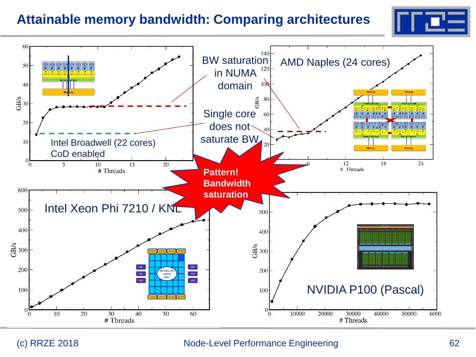
Attainable memory bandwidth: Comparing architectures
(c) RRZE 2018 Node-Level Performance Engineering
Intel Broadwell (22 cores)
CoD enabled
AMD Naples (24 cores)
ECC=on
Single core
does not
saturate BW
BW saturation
in NUMA
domain
Intel Xeon Phi 7210 / KNL
NVIDIA P100 (Pascal)
MCDRAM MCDRAM MCDRAM MCDRAM
MCDRAM MCDRAM MCDRAM MCDRAM
DDR4
DDR4
DDR4
DDR4
DDR4
DDR4
36 tiles (72
cores)
max.
Pattern!
Bandwidth
saturation
64
Conclusions from the microbenchmarks
Affinity matters!
Almost all performance properties depend on the position of
Data
Threads/processes
Consequences
Know where your threads are running
Know where your data is
Bandwidth bottlenecks are ubiquitous
(c) RRZE 2018 Node-Level Performance Engineering
“Simple” performance modeling:
The Roofline Model
Loop-based performance modeling: Execution vs. data transfer
Example: array summation
Example: dense & sparse matrix-vector multiplication
Example: a 3D Jacobi solver
Model-guided optimization
R.W. Hockney and I.J. Curington: f1/2: A parameter to characterize memory and communication bottlenecks.
Parallel Computing 10, 277-286 (1989). DOI: 10.1016/0167-8191(89)90100-2
W. Schönauer: Scientific Supercomputing: Architecture and Use of Shared and Distributed Memory Parallel Computers.
Self-edition (2000)
S. Williams: Auto-tuning Performance on Multicore Computers.
UCB Technical Report No. UCB/EECS-2008-164. PhD thesis (2008)
66
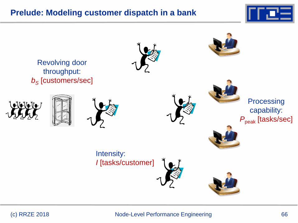
Prelude: Modeling customer dispatch in a bank
(c) RRZE 2018 Node-Level Performance Engineering
Revolving door
throughput:
bS [customers/sec]
Intensity:
I [tasks/customer]
Processing
capability:
Ppeak [tasks/sec]
67
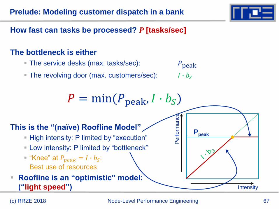
Prelude: Modeling customer dispatch in a bank
How fast can tasks be processed? 𝑷 [tasks/sec]
The bottleneck is either
The service desks (max. tasks/sec): 𝑃peak
The revolving door (max. customers/sec): 𝐼 ∙ 𝑏𝑆
This is the “(naïve) Roofline Model”
High intensity: P limited by “execution”
Low intensity: P limited by “bottleneck”
“Knee” at 𝑃𝑝𝑒𝑎𝑘 = 𝐼 ∙ 𝑏𝑆:
Best use of resources
Roofline is an “optimistic” model:
(“light speed”)
(c) RRZE 2018 Node-Level Performance Engineering
𝑃 = min(𝑃peak, 𝐼 ∙ 𝑏𝑆)
Intensity
Perf
orm
ance
Ppeak
68
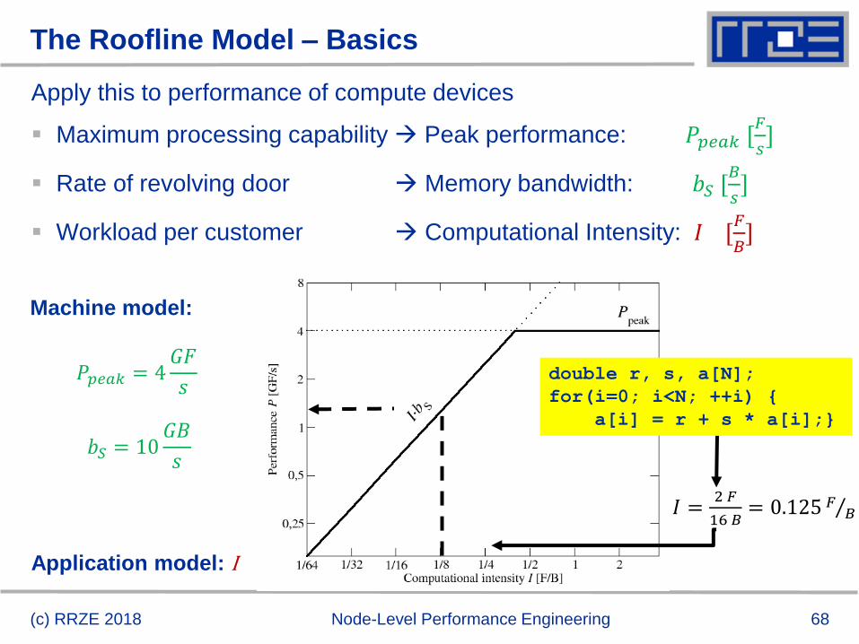
Apply this to performance of compute devices
Maximum processing capability Peak performance: 𝑃𝑝𝑒𝑎𝑘 [𝐹
𝑠]
Rate of revolving door Memory bandwidth: 𝑏𝑆 [𝐵
𝑠]
Workload per customer Computational Intensity: 𝐼 [𝐹
𝐵]
The Roofline Model – Basics
(c) RRZE 2018 Node-Level Performance Engineering
Machine model:
𝑃𝑝𝑒𝑎𝑘 = 4𝐺𝐹
𝑠
𝑏𝑆 = 10𝐺𝐵
𝑠
Application model: I
double r, s, a[N];
for(i=0; i<N; ++i) {
a[i] = r + s * a[i];}
𝐼 =2 𝐹
16 𝐵= 0.125 Τ𝐹 𝐵
69
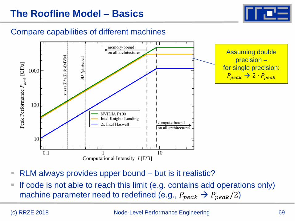
The Roofline Model – Basics
Compare capabilities of different machines
RLM always provides upper bound – but is it realistic?
If code is not able to reach this limit (e.g. contains add operations only)
machine parameter need to redefined (e.g., 𝑃𝑝𝑒𝑎𝑘 𝑃𝑝𝑒𝑎𝑘/2)
(c) RRZE 2018 Node-Level Performance Engineering
Assuming double
precision –
for single precision:
𝑃𝑝𝑒𝑎𝑘 2 ∙ 𝑃𝑝𝑒𝑎𝑘
70
The Roofline Model
(a slightly refined version for better in-core prediction)
(c) RRZE 2018 Node-Level Performance Engineering
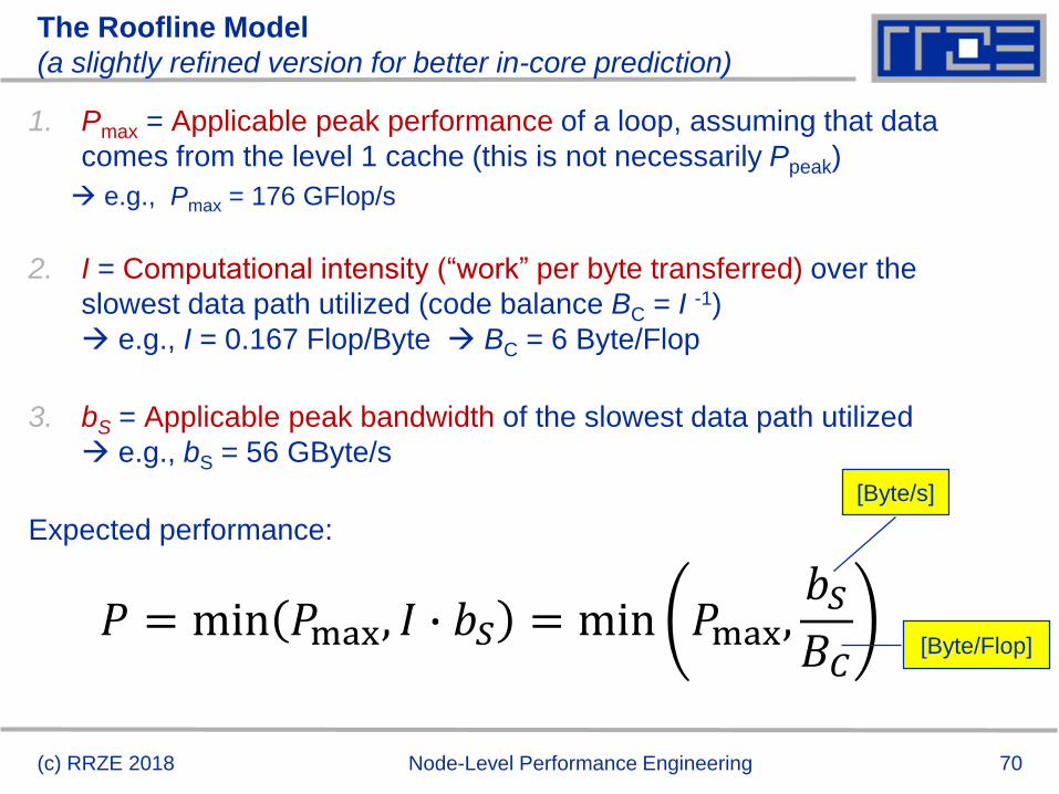
1. Pmax = Applicable peak performance of a loop, assuming that data
comes from the level 1 cache (this is not necessarily Ppeak)
e.g., Pmax = 176 GFlop/s
2. I = Computational intensity (“work” per byte transferred) over the
slowest data path utilized (code balance BC = I -1)
e.g., I = 0.167 Flop/Byte BC = 6 Byte/Flop
3. bS = Applicable peak bandwidth of the slowest data path utilized
e.g., bS = 56 GByte/s
Expected performance:
𝑃 = min 𝑃max, 𝐼 ∙ 𝑏𝑆 = min 𝑃max,𝑏𝑆𝐵𝐶
[Byte/s]
[Byte/Flop]
71
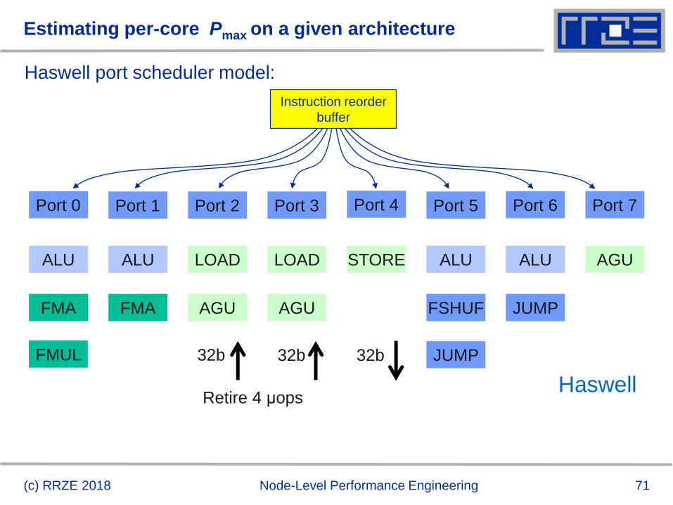
Estimating per-core Pmax on a given architecture
Haswell port scheduler model:
Port 0 Port 1 Port 5Port 2 Port 3 Port 4 Port 6 Port 7
ALU ALU ALU
FMA FMA FSHUF
JUMP
LOAD LOAD
AGU AGU
STORE
Retire 4 μops
32b 32b 32b
AGU
Haswell
FMUL
ALU
JUMP
(c) RRZE 2018 Node-Level Performance Engineering
Instruction reorder
buffer
72
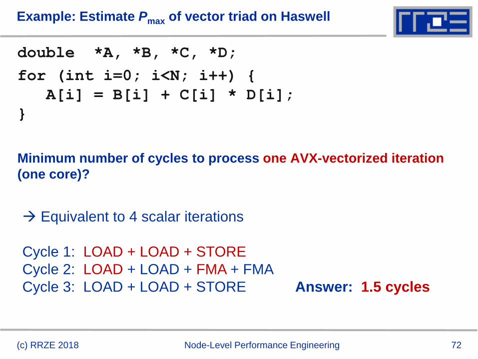
Example: Estimate Pmax of vector triad on Haswell
double *A, *B, *C, *D;
for (int i=0; i<N; i++) {
A[i] = B[i] + C[i] * D[i];
}
Minimum number of cycles to process one AVX-vectorized iteration
(one core)?
Equivalent to 4 scalar iterations
Cycle 1: LOAD + LOAD + STORE
Cycle 2: LOAD + LOAD + FMA + FMA
Cycle 3: LOAD + LOAD + STORE Answer: 1.5 cycles
(c) RRZE 2018 Node-Level Performance Engineering
73
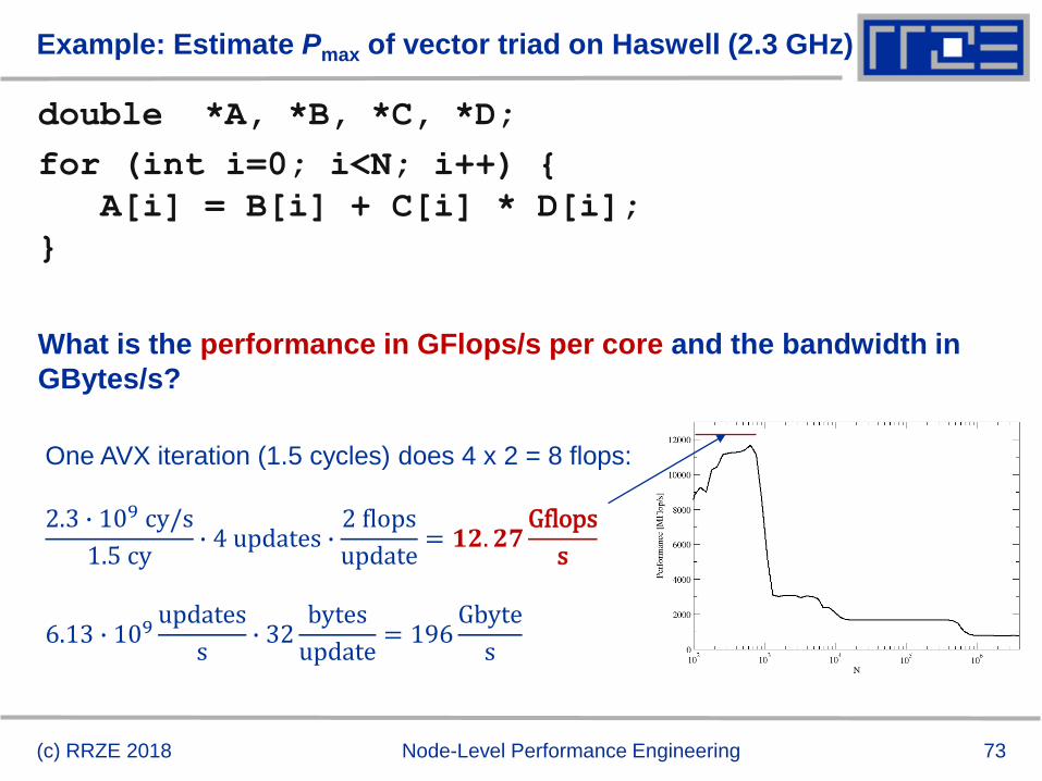
Example: Estimate Pmax of vector triad on Haswell (2.3 GHz)
double *A, *B, *C, *D;
for (int i=0; i<N; i++) {
A[i] = B[i] + C[i] * D[i];
}
What is the performance in GFlops/s per core and the bandwidth in
GBytes/s?
One AVX iteration (1.5 cycles) does 4 x 2 = 8 flops:
2.3 ∙ 109 cy/s
1.5 cy∙ 4 updates ∙
2 flops
update= 𝟏𝟐. 𝟐𝟕
Gflops
s
6.13 ∙ 109updates
s∙ 32
bytes
update= 196
Gbyte
s
(c) RRZE 2018 Node-Level Performance Engineering
74
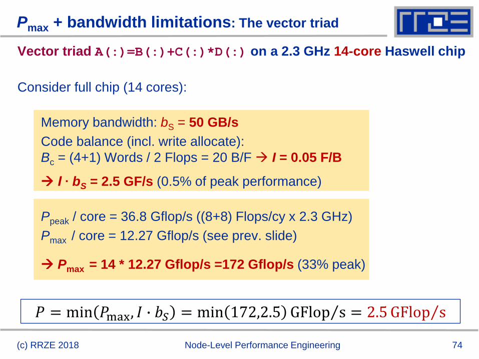
Pmax + bandwidth limitations: The vector triad
Vector triad A(:)=B(:)+C(:)*D(:) on a 2.3 GHz 14-core Haswell chip
Consider full chip (14 cores):
Memory bandwidth: bS = 50 GB/s
Code balance (incl. write allocate):
Bc = (4+1) Words / 2 Flops = 20 B/F I = 0.05 F/B
I ∙ bS = 2.5 GF/s (0.5% of peak performance)
Ppeak / core = 36.8 Gflop/s ((8+8) Flops/cy x 2.3 GHz)
Pmax / core = 12.27 Gflop/s (see prev. slide)
Pmax = 14 * 12.27 Gflop/s =172 Gflop/s (33% peak)
𝑃 = min 𝑃max, 𝐼 ∙ 𝑏𝑆 = min 172,2.5 ΤGFlop s = 2.5 ΤGFlop s
(c) RRZE 2018 Node-Level Performance Engineering
75
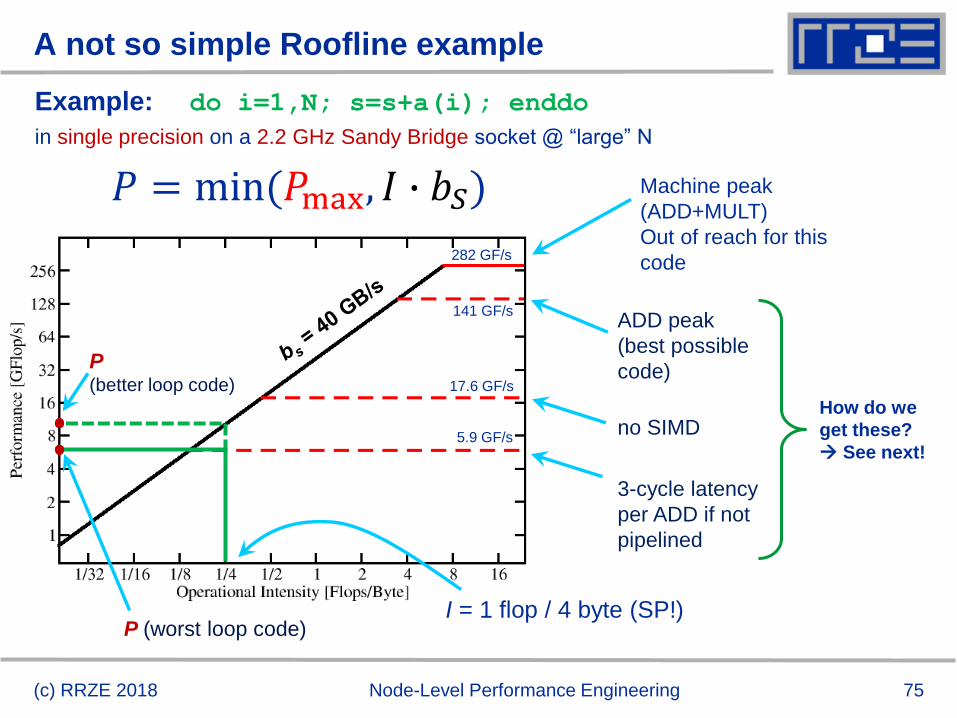
A not so simple Roofline example
Example: do i=1,N; s=s+a(i); enddo
in single precision on a 2.2 GHz Sandy Bridge socket @ “large” N
(c) RRZE 2018 Node-Level Performance Engineering
ADD peak
(best possible
code)
no SIMD
3-cycle latency
per ADD if not
pipelined
P (worst loop code)
𝑃 = min(𝑃max, 𝐼 ∙ 𝑏𝑆)
How do we
get these?
See next!
I = 1 flop / 4 byte (SP!)
141 GF/s
17.6 GF/s
5.9 GF/s
282 GF/s
Machine peak
(ADD+MULT)
Out of reach for this
code
P (better loop code)
76
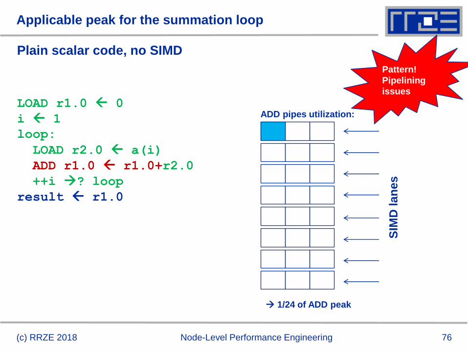
Applicable peak for the summation loop
Plain scalar code, no SIMD
LOAD r1.0 0
i 1
loop:
LOAD r2.0 a(i)
ADD r1.0 r1.0+r2.0
++i ? loop
result r1.0
(c) RRZE 2018 Node-Level Performance Engineering
ADD pipes utilization:
1/24 of ADD peak
SIM
D lan
es
Pattern!
Pipelining
issues
77
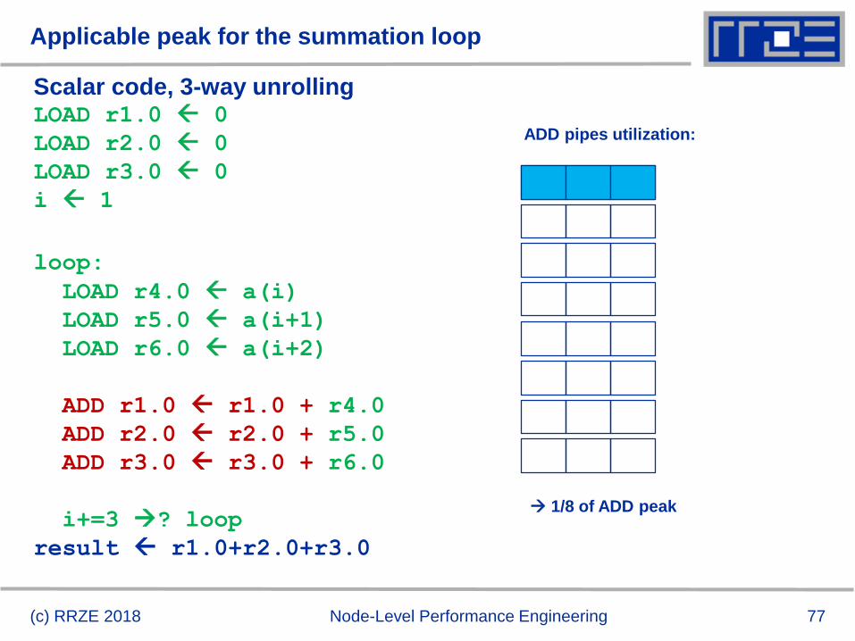
Applicable peak for the summation loop
Scalar code, 3-way unrollingLOAD r1.0 0
LOAD r2.0 0
LOAD r3.0 0
i 1
loop:
LOAD r4.0 a(i)
LOAD r5.0 a(i+1)
LOAD r6.0 a(i+2)
ADD r1.0 r1.0 + r4.0
ADD r2.0 r2.0 + r5.0
ADD r3.0 r3.0 + r6.0
i+=3 ? loop
result r1.0+r2.0+r3.0
(c) RRZE 2018 Node-Level Performance Engineering
ADD pipes utilization:
1/8 of ADD peak
78
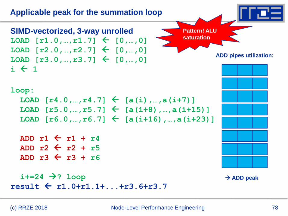
Applicable peak for the summation loop
SIMD-vectorized, 3-way unrolledLOAD [r1.0,…,r1.7] [0,…,0]
LOAD [r2.0,…,r2.7] [0,…,0]
LOAD [r3.0,…,r3.7] [0,…,0]
i 1
loop:
LOAD [r4.0,…,r4.7] [a(i),…,a(i+7)]
LOAD [r5.0,…,r5.7] [a(i+8),…,a(i+15)]
LOAD [r6.0,…,r6.7] [a(i+16),…,a(i+23)]
ADD r1 r1 + r4
ADD r2 r2 + r5
ADD r3 r3 + r6
i+=24 ? loop
result r1.0+r1.1+...+r3.6+r3.7
(c) RRZE 2018 Node-Level Performance Engineering
ADD pipes utilization:
ADD peak
Pattern! ALU
saturation
79
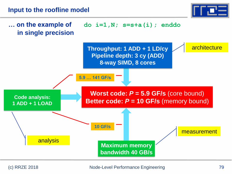
Input to the roofline model
… on the example of do i=1,N; s=s+a(i); enddo
in single precision
(c) RRZE 2018 Node-Level Performance Engineering
analysis
Code analysis:
1 ADD + 1 LOAD
architectureThroughput: 1 ADD + 1 LD/cy
Pipeline depth: 3 cy (ADD)
8-way SIMD, 8 cores
measurement
Maximum memory
bandwidth 40 GB/s
Worst code: P = 5.9 GF/s (core bound)
Better code: P = 10 GF/s (memory bound)
5.9 … 141 GF/s
10 GF/s
80
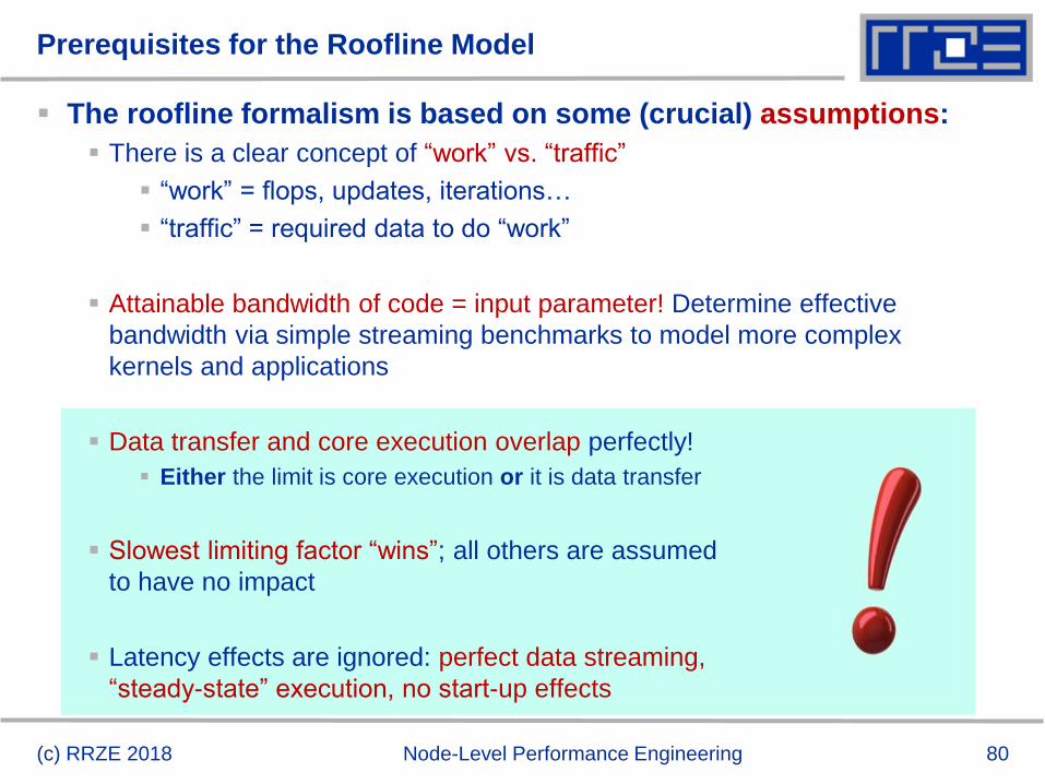
Prerequisites for the Roofline Model
(c) RRZE 2018 Node-Level Performance Engineering
The roofline formalism is based on some (crucial) assumptions:
There is a clear concept of “work” vs. “traffic”
“work” = flops, updates, iterations…
“traffic” = required data to do “work”
Attainable bandwidth of code = input parameter! Determine effective
bandwidth via simple streaming benchmarks to model more complex
kernels and applications
Data transfer and core execution overlap perfectly!
Either the limit is core execution or it is data transfer
Slowest limiting factor “wins”; all others are assumed
to have no impact
Latency effects are ignored: perfect data streaming,
“steady-state” execution, no start-up effects
Multicore performance tools:
Probing performance behavior
likwid-perfctr
83(c) RRZE 2018 Node-Level Performance Engineering
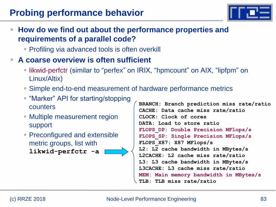
Probing performance behavior
How do we find out about the performance properties and
requirements of a parallel code?
Profiling via advanced tools is often overkill
A coarse overview is often sufficient
likwid-perfctr (similar to “perfex” on IRIX, “hpmcount” on AIX, “lipfpm” on
Linux/Altix)
Simple end-to-end measurement of hardware performance metrics
“Marker” API for starting/stopping
counters
Multiple measurement region
support
Preconfigured and extensible
metric groups, list withlikwid-perfctr -a
BRANCH: Branch prediction miss rate/ratio
CACHE: Data cache miss rate/ratio
CLOCK: Clock of cores
DATA: Load to store ratio
FLOPS_DP: Double Precision MFlops/s
FLOPS_SP: Single Precision MFlops/s
FLOPS_X87: X87 MFlops/s
L2: L2 cache bandwidth in MBytes/s
L2CACHE: L2 cache miss rate/ratio
L3: L3 cache bandwidth in MBytes/s
L3CACHE: L3 cache miss rate/ratio
MEM: Main memory bandwidth in MBytes/s
TLB: TLB miss rate/ratio
84(c) RRZE 2018 Node-Level Performance Engineering
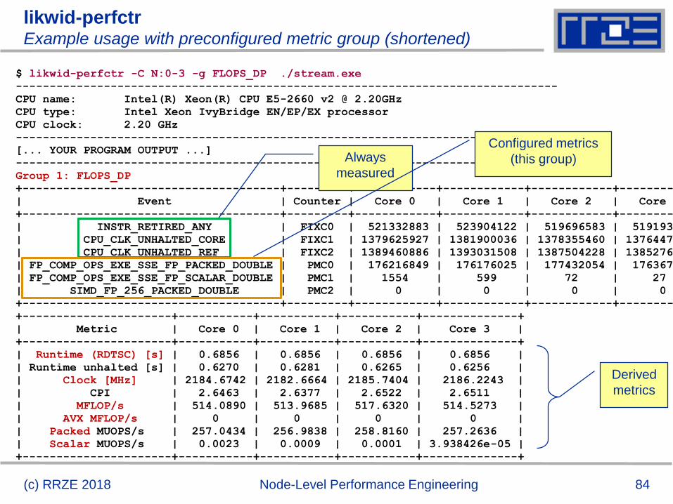
likwid-perfctrExample usage with preconfigured metric group (shortened)
$ likwid-perfctr -C N:0-3 -g FLOPS_DP ./stream.exe
--------------------------------------------------------------------------------
CPU name: Intel(R) Xeon(R) CPU E5-2660 v2 @ 2.20GHz
CPU type: Intel Xeon IvyBridge EN/EP/EX processor
CPU clock: 2.20 GHz
--------------------------------------------------------------------------------
[... YOUR PROGRAM OUTPUT ...]
--------------------------------------------------------------------------------
Group 1: FLOPS_DP
+--------------------------------------+---------+------------+------------+------------+------------
| Event | Counter | Core 0 | Core 1 | Core 2 | Core 3 |
+--------------------------------------+---------+------------+------------+------------+------------
| INSTR_RETIRED_ANY | FIXC0 | 521332883 | 523904122 | 519696583 | 519193735 |
| CPU_CLK_UNHALTED_CORE | FIXC1 | 1379625927 | 1381900036 | 1378355460 | 1376447129 |
| CPU_CLK_UNHALTED_REF | FIXC2 | 1389460886 | 1393031508 | 1387504228 | 1385276552 |
| FP_COMP_OPS_EXE_SSE_FP_PACKED_DOUBLE | PMC0 | 176216849 | 176176025 | 177432054 | 176367855 |
| FP_COMP_OPS_EXE_SSE_FP_SCALAR_DOUBLE | PMC1 | 1554 | 599 | 72 | 27 |
| SIMD_FP_256_PACKED_DOUBLE | PMC2 | 0 | 0 | 0 | 0 |
+--------------------------------------+---------+------------+------------+------------+------------
+----------------------+-----------+-----------+-----------+--------------+
| Metric | Core 0 | Core 1 | Core 2 | Core 3 |
+----------------------+-----------+-----------+-----------+--------------+
| Runtime (RDTSC) [s] | 0.6856 | 0.6856 | 0.6856 | 0.6856 |
| Runtime unhalted [s] | 0.6270 | 0.6281 | 0.6265 | 0.6256 |
| Clock [MHz] | 2184.6742 | 2182.6664 | 2185.7404 | 2186.2243 |
| CPI | 2.6463 | 2.6377 | 2.6522 | 2.6511 |
| MFLOP/s | 514.0890 | 513.9685 | 517.6320 | 514.5273 |
| AVX MFLOP/s | 0 | 0 | 0 | 0 |
| Packed MUOPS/s | 257.0434 | 256.9838 | 258.8160 | 257.2636 |
| Scalar MUOPS/s | 0.0023 | 0.0009 | 0.0001 | 3.938426e-05 |
+----------------------+-----------+-----------+-----------+--------------+
Derived
metrics
Always
measured
Configured metrics
(this group)
85
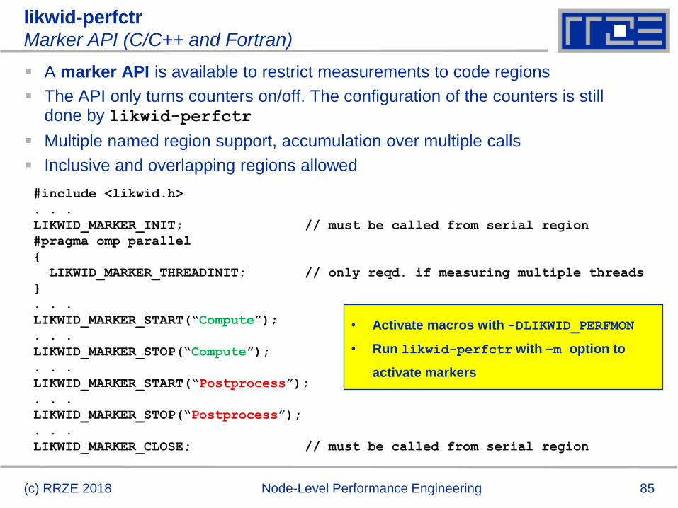
likwid-perfctr
Marker API (C/C++ and Fortran)
A marker API is available to restrict measurements to code regions
The API only turns counters on/off. The configuration of the counters is still done by likwid-perfctr
Multiple named region support, accumulation over multiple calls
Inclusive and overlapping regions allowed
(c) RRZE 2018
#include <likwid.h>
. . .
LIKWID_MARKER_INIT; // must be called from serial region
#pragma omp parallel
{
LIKWID_MARKER_THREADINIT; // only reqd. if measuring multiple threads
}
. . .
LIKWID_MARKER_START(“Compute”);
. . .
LIKWID_MARKER_STOP(“Compute”);
. . .
LIKWID_MARKER_START(“Postprocess”);
. . .
LIKWID_MARKER_STOP(“Postprocess”);
. . .
LIKWID_MARKER_CLOSE; // must be called from serial region
Node-Level Performance Engineering
• Activate macros with -DLIKWID_PERFMON
• Run likwid-perfctr with –m option to
activate markers
86
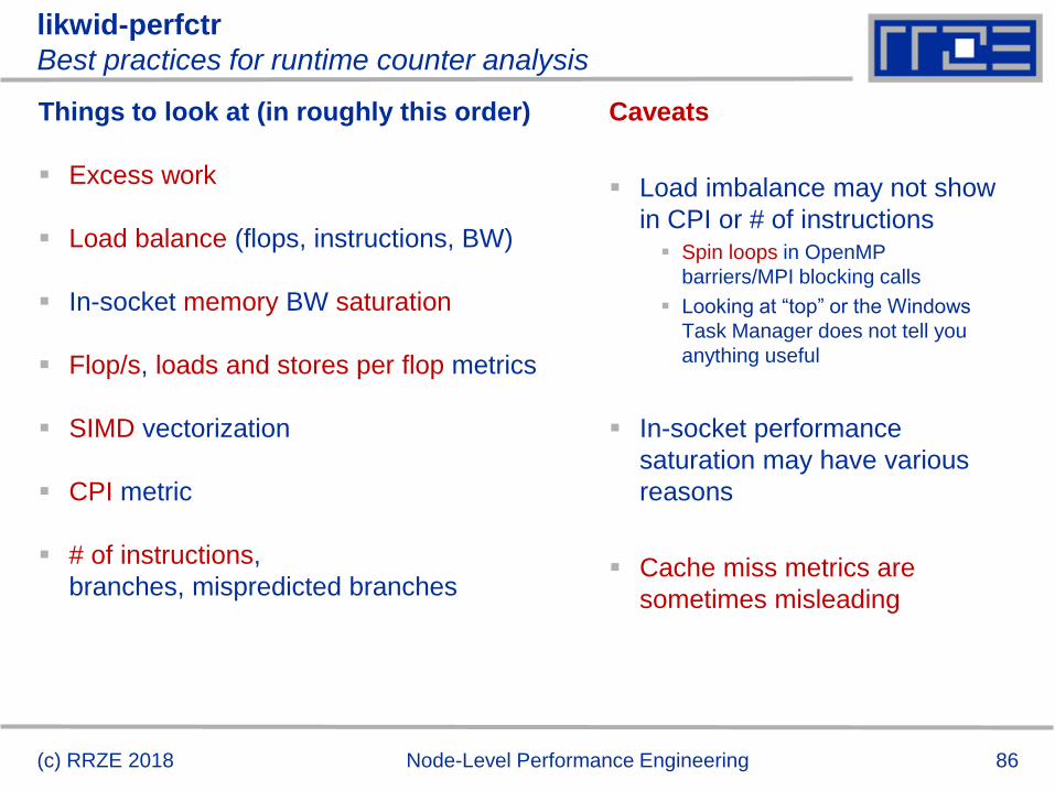
likwid-perfctr
Best practices for runtime counter analysis
Things to look at (in roughly this order)
Excess work
Load balance (flops, instructions, BW)
In-socket memory BW saturation
Flop/s, loads and stores per flop metrics
SIMD vectorization
CPI metric
# of instructions,
branches, mispredicted branches
Caveats
Load imbalance may not show
in CPI or # of instructions Spin loops in OpenMP
barriers/MPI blocking calls
Looking at “top” or the Windows
Task Manager does not tell you
anything useful
In-socket performance
saturation may have various
reasons
Cache miss metrics are
sometimes misleading
(c) RRZE 2018 Node-Level Performance Engineering
Measuring energy consumption
with LIKWID
88
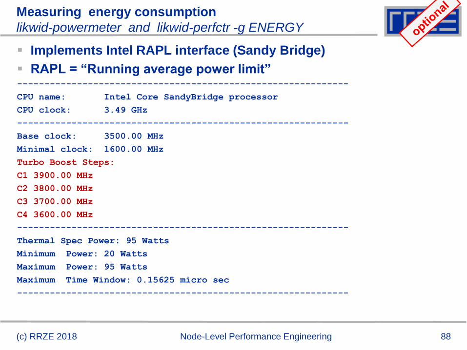
Measuring energy consumption
likwid-powermeter and likwid-perfctr -g ENERGY
Implements Intel RAPL interface (Sandy Bridge)
RAPL = “Running average power limit”-------------------------------------------------------------
CPU name: Intel Core SandyBridge processor
CPU clock: 3.49 GHz
-------------------------------------------------------------
Base clock: 3500.00 MHz
Minimal clock: 1600.00 MHz
Turbo Boost Steps:
C1 3900.00 MHz
C2 3800.00 MHz
C3 3700.00 MHz
C4 3600.00 MHz
-------------------------------------------------------------
Thermal Spec Power: 95 Watts
Minimum Power: 20 Watts
Maximum Power: 95 Watts
Maximum Time Window: 0.15625 micro sec
-------------------------------------------------------------
(c) RRZE 2018 Node-Level Performance Engineering
89
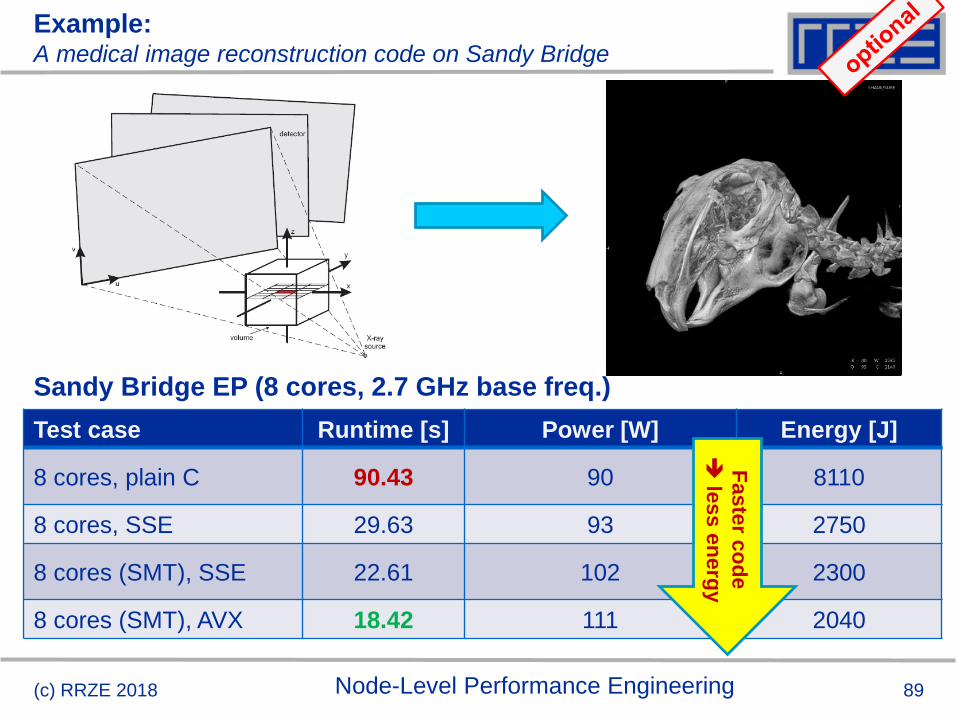
Example:A medical image reconstruction code on Sandy Bridge
(c) RRZE 2018 Node-Level Performance Engineering
Test case Runtime [s] Power [W] Energy [J]
8 cores, plain C 90.43 90 8110
8 cores, SSE 29.63 93 2750
8 cores (SMT), SSE 22.61 102 2300
8 cores (SMT), AVX 18.42 111 2040
Sandy Bridge EP (8 cores, 2.7 GHz base freq.)
Faste
r co
de
le
ss e
ne
rgy
90
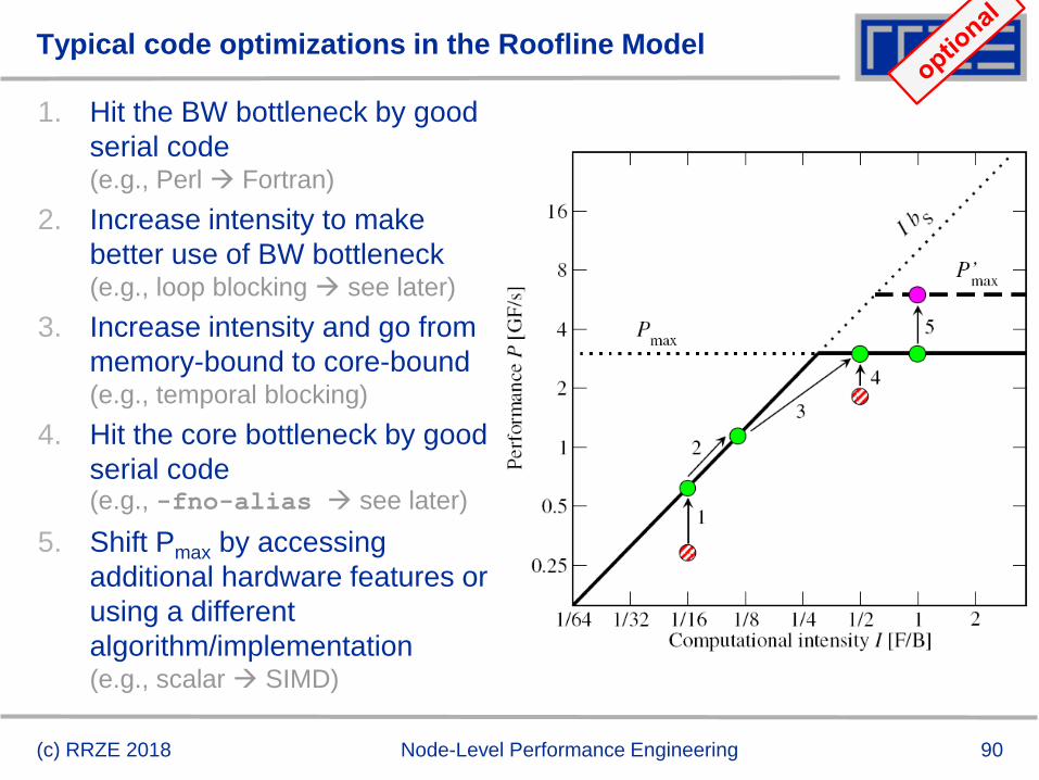
Typical code optimizations in the Roofline Model
1. Hit the BW bottleneck by good
serial code(e.g., Perl Fortran)
2. Increase intensity to make
better use of BW bottleneck(e.g., loop blocking see later)
3. Increase intensity and go from
memory-bound to core-bound(e.g., temporal blocking)
4. Hit the core bottleneck by good
serial code(e.g., -fno-alias see later)
5. Shift Pmax by accessing
additional hardware features or
using a different
algorithm/implementation(e.g., scalar SIMD)
(c) RRZE 2018 Node-Level Performance Engineering
91
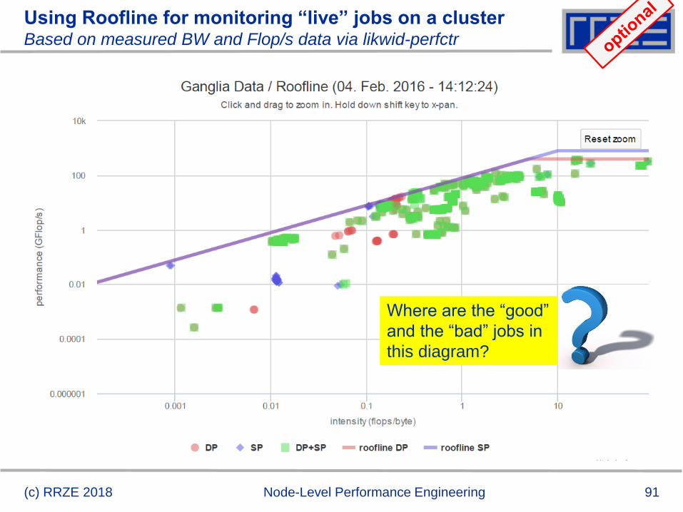
Using Roofline for monitoring “live” jobs on a clusterBased on measured BW and Flop/s data via likwid-perfctr
(c) RRZE 2018 Node-Level Performance Engineering
Where are the “good”
and the “bad” jobs in
this diagram?
Case study: A Jacobi smoother
The basic performance properties in 2D
Layer conditions
Optimization by spatial blocking
93
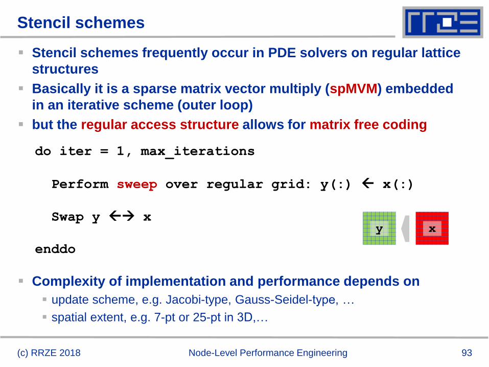
Stencil schemes
Stencil schemes frequently occur in PDE solvers on regular lattice
structures
Basically it is a sparse matrix vector multiply (spMVM) embedded
in an iterative scheme (outer loop)
but the regular access structure allows for matrix free coding
Complexity of implementation and performance depends on
update scheme, e.g. Jacobi-type, Gauss-Seidel-type, …
spatial extent, e.g. 7-pt or 25-pt in 3D,…
(c) RRZE 2018 Node-Level Performance Engineering
do iter = 1, max_iterations
Perform sweep over regular grid: y(:) x(:)
Swap y x
enddo
y x
94
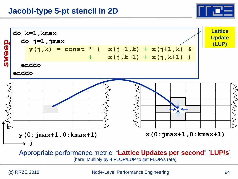
Jacobi-type 5-pt stencil in 2D
(c) RRZE 2018 Node-Level Performance Engineering
do k=1,kmax
do j=1,jmax
y(j,k) = const * ( x(j-1,k) + x(j+1,k) &
+ x(j,k-1) + x(j,k+1) )
enddo
enddo
j
k
sweep
Lattice
Update
(LUP)
y(0:jmax+1,0:kmax+1) x(0:jmax+1,0:kmax+1)
Appropriate performance metric: “Lattice Updates per second” [LUP/s](here: Multiply by 4 FLOP/LUP to get FLOP/s rate)
95
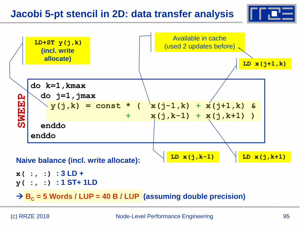
Jacobi 5-pt stencil in 2D: data transfer analysis
(c) RRZE 2018 Node-Level Performance Engineering
do k=1,kmax
do j=1,jmax
y(j,k) = const * ( x(j-1,k) + x(j+1,k) &
+ x(j,k-1) + x(j,k+1) )
enddo
enddo
SWEEP
LD+ST y(j,k)
(incl. write
allocate)LD x(j+1,k)
Available in cache
(used 2 updates before)
LD x(j,k+1)LD x(j,k-1)Naive balance (incl. write allocate):
x( :, :) : 3 LD +
y( :, :) : 1 ST+ 1LD
BC = 5 Words / LUP = 40 B / LUP (assuming double precision)
96
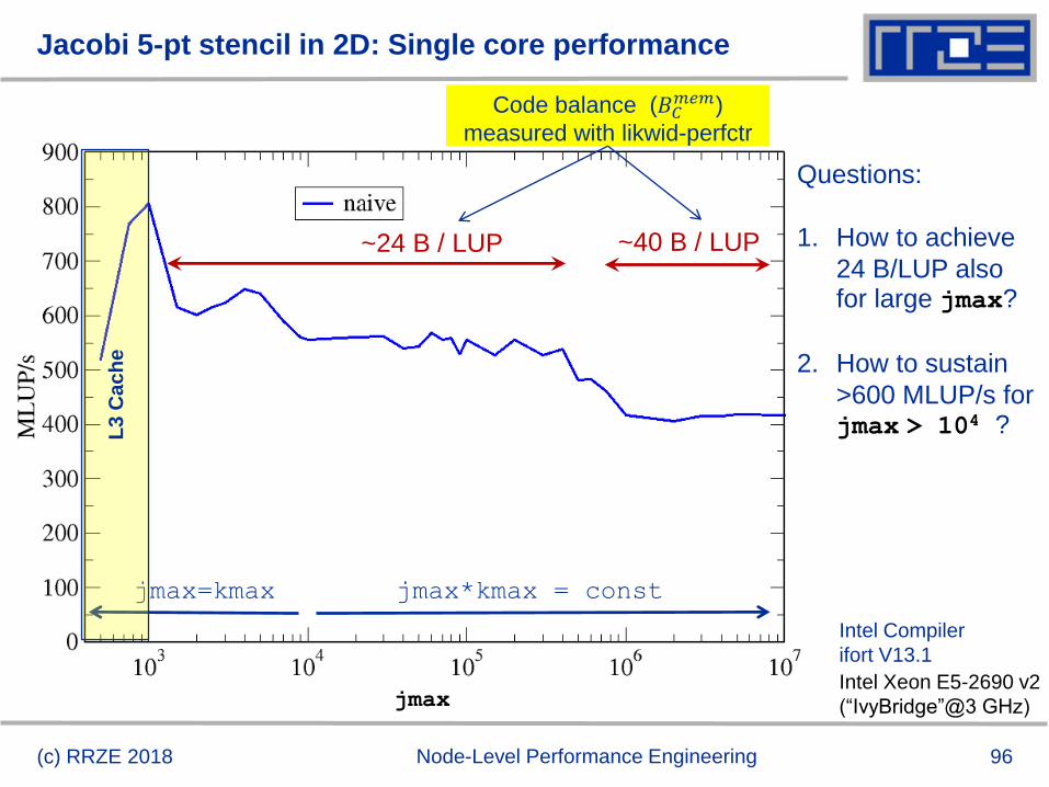
Jacobi 5-pt stencil in 2D: Single core performance
(c) RRZE 2018 Node-Level Performance Engineering
jmax=kmax jmax*kmax = const
L3
Ca
ch
e
Intel Xeon E5-2690 v2
(“IvyBridge”@3 GHz)
~24 B / LUP ~40 B / LUP
Code balance (𝐵𝐶𝑚𝑒𝑚)
measured with likwid-perfctr
Intel Compiler
ifort V13.1
jmax
Questions:
1. How to achieve
24 B/LUP also for large jmax?
2. How to sustain
>600 MLUP/s for jmax > 104 ?
Case study: A Jacobi smoother
The basics in two dimensions
Layer conditions
Optimization by spatial blocking
98
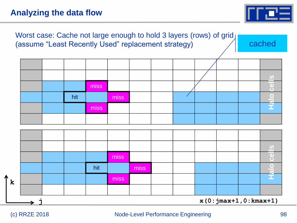
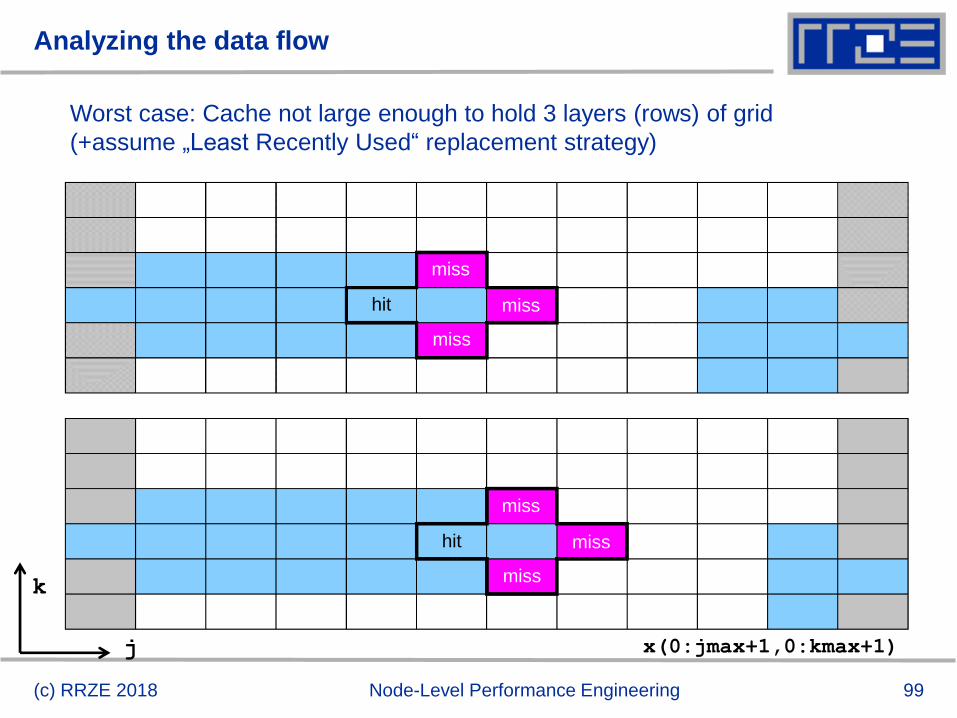
Analyzing the data flow
(c) RRZE 2018 Node-Level Performance Engineering
cachedWorst case: Cache not large enough to hold 3 layers (rows) of grid
(assume “Least Recently Used” replacement strategy)
j
k
x(0:jmax+1,0:kmax+1)
Halo
cell
sH
alo
cell
s
miss
miss
miss
hit
miss
miss
miss
hit
99
Analyzing the data flow
(c) RRZE 2018 Node-Level Performance Engineering
j
k
Worst case: Cache not large enough to hold 3 layers (rows) of grid
(+assume „Least Recently Used“ replacement strategy)
x(0:jmax+1,0:kmax+1)
miss
miss
miss
hit
miss
miss
miss
hit
100
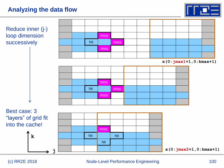
Analyzing the data flow
(c) RRZE 2018 Node-Level Performance Engineering
Reduce inner (j-)
loop dimension
successively
Best case: 3
“layers” of grid fit
into the cache!
j
k
x(0:jmax2+1,0:kmax+1)
x(0:jmax1+1,0:kmax+1)
miss
miss
miss
hit
miss
miss
miss
hit
miss
hit
hit
hit
101
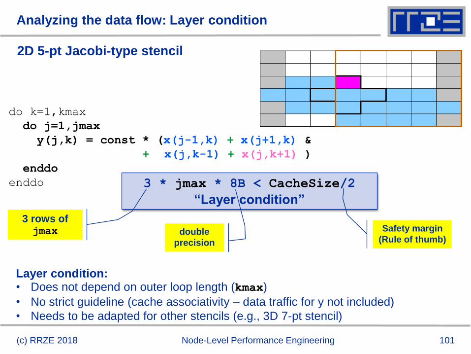
Analyzing the data flow: Layer condition
2D 5-pt Jacobi-type stencil
(c) RRZE 2018 Node-Level Performance Engineering
do k=1,kmax
do j=1,jmax
y(j,k) = const * (x(j-1,k) + x(j+1,k) &
+ x(j,k-1) + x(j,k+1) )
enddo
enddo 3 * jmax * 8B < CacheSize/2
“Layer condition”
double
precision
3 rows of jmax Safety margin
(Rule of thumb)
Layer condition:• Does not depend on outer loop length (kmax)
• No strict guideline (cache associativity – data traffic for y not included)
• Needs to be adapted for other stencils (e.g., 3D 7-pt stencil)
102
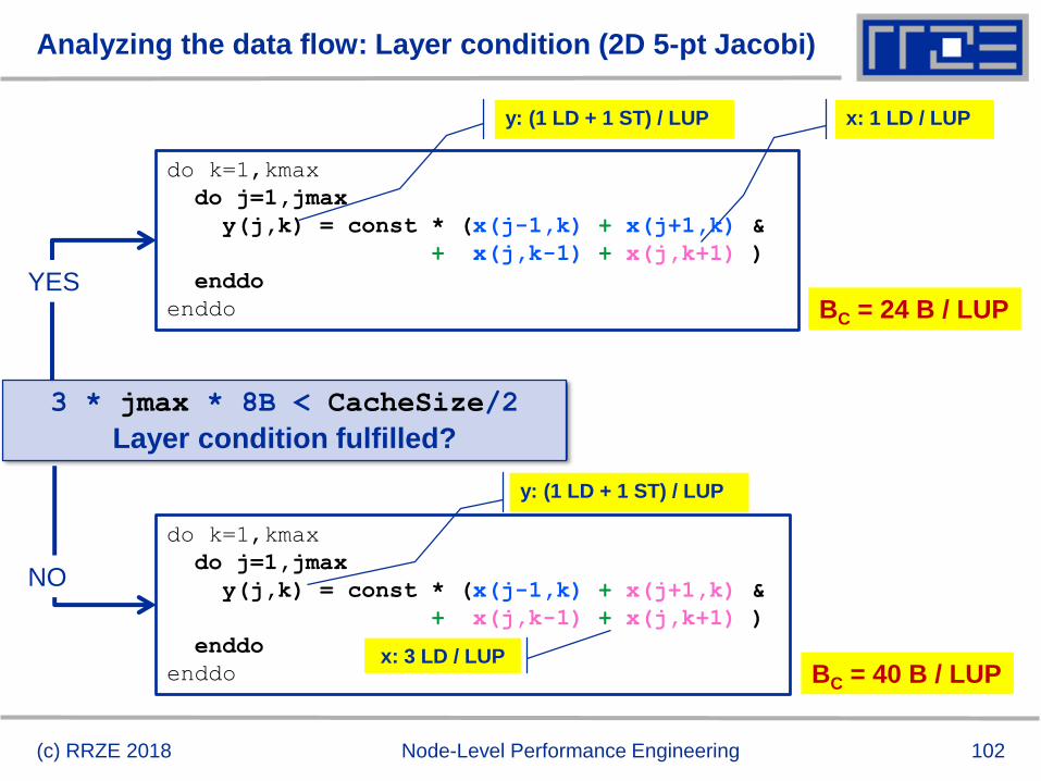
Analyzing the data flow: Layer condition (2D 5-pt Jacobi)
(c) RRZE 2018 Node-Level Performance Engineering
3 * jmax * 8B < CacheSize/2
Layer condition fulfilled?
y: (1 LD + 1 ST) / LUP x: 1 LD / LUP
BC = 24 B / LUP
do k=1,kmax
do j=1,jmax
y(j,k) = const * (x(j-1,k) + x(j+1,k) &
+ x(j,k-1) + x(j,k+1) )
enddo
enddo
YES
do k=1,kmax
do j=1,jmax
y(j,k) = const * (x(j-1,k) + x(j+1,k) &
+ x(j,k-1) + x(j,k+1) )
enddo
enddo BC = 40 B / LUP
y: (1 LD + 1 ST) / LUP
NO
x: 3 LD / LUP
103
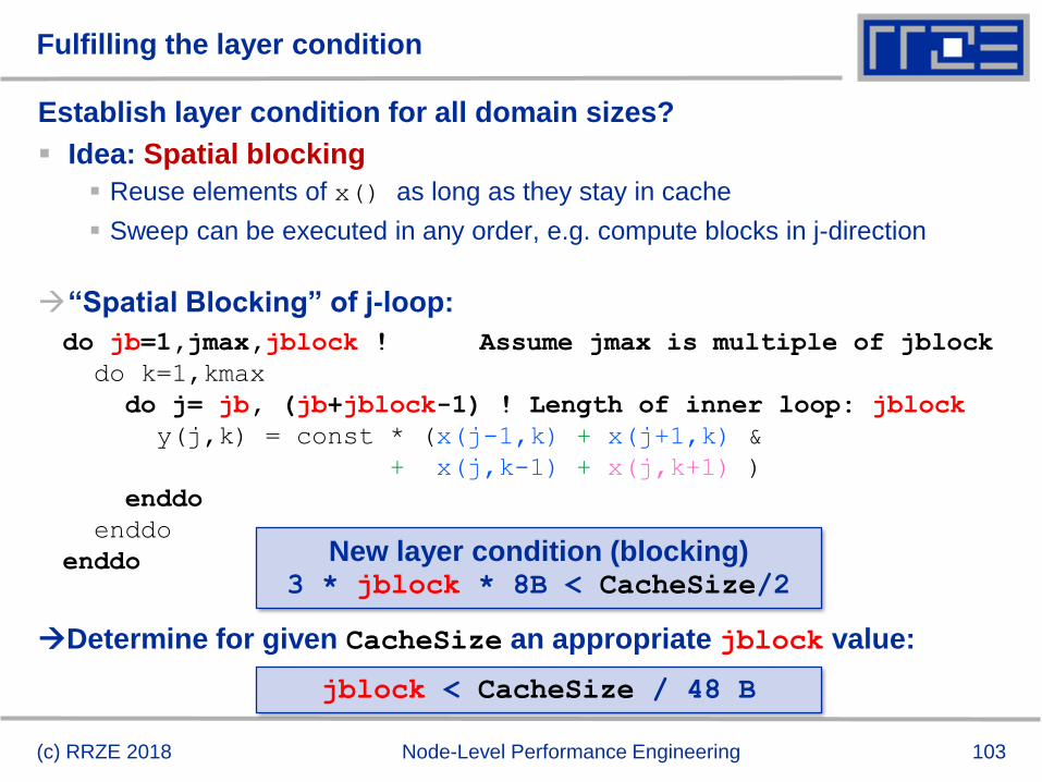
Fulfilling the layer condition
Establish layer condition for all domain sizes?
Idea: Spatial blocking
Reuse elements of x() as long as they stay in cache
Sweep can be executed in any order, e.g. compute blocks in j-direction
“Spatial Blocking” of j-loop:
Determine for given CacheSize an appropriate jblock value:
(c) RRZE 2018 Node-Level Performance Engineering
do jb=1,jmax,jblock ! Assume jmax is multiple of jblock
do k=1,kmax
do j= jb, (jb+jblock-1) ! Length of inner loop: jblock
y(j,k) = const * (x(j-1,k) + x(j+1,k) &
+ x(j,k-1) + x(j,k+1) )
enddo
enddo
enddo New layer condition (blocking)3 * jblock * 8B < CacheSize/2
jblock < CacheSize / 48 B
104
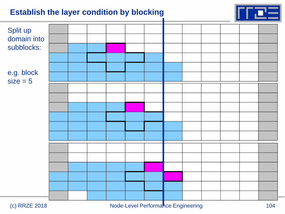
Establish the layer condition by blocking
(c) RRZE 2018 Node-Level Performance Engineering
Split up
domain into
subblocks:
e.g. block
size = 5
105
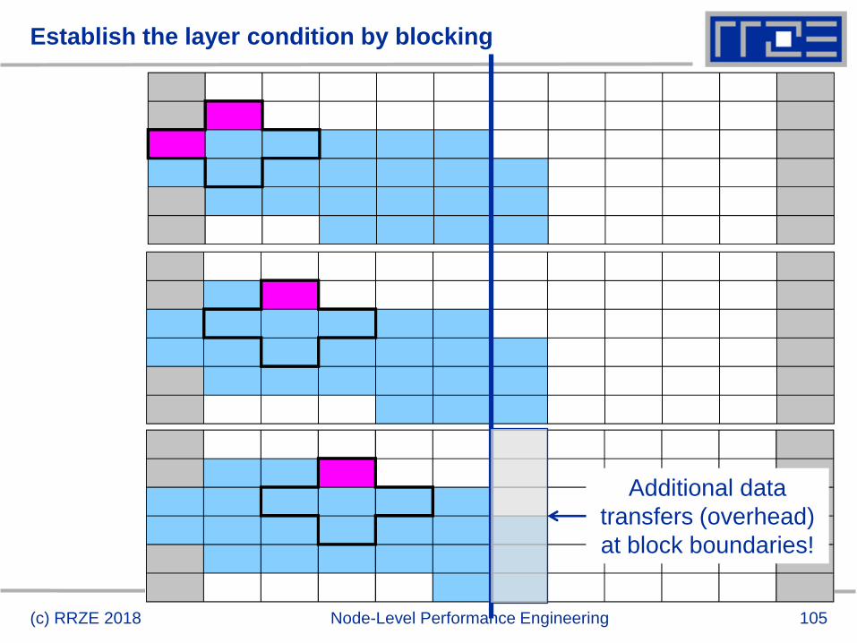
Establish the layer condition by blocking
(c) RRZE 2018 Node-Level Performance Engineering
Additional data
transfers (overhead)
at block boundaries!
106
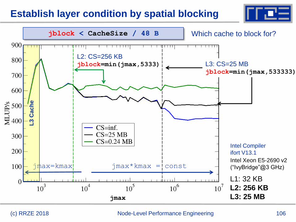
Establish layer condition by spatial blocking
(c) RRZE 2018 Node-Level Performance Engineering
jmax=kmax jmax*kmax = const
L3
Ca
ch
e
L1: 32 KB
L2: 256 KB
L3: 25 MBjmax
Which cache to block for?
Intel Xeon E5-2690 v2
(“IvyBridge”@3 GHz)
Intel Compiler
ifort V13.1
jblock < CacheSize / 48 B
L2: CS=256 KBjblock=min(jmax,5333) L3: CS=25 MB
jblock=min(jmax,533333)
107
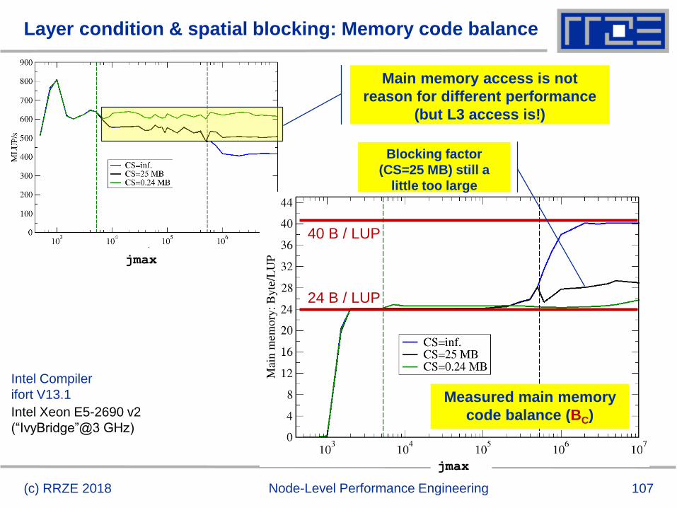
Layer condition & spatial blocking: Memory code balance
(c) RRZE 2018 Node-Level Performance Engineering
jmax
Measured main memory
code balance (BC)
24 B / LUP
40 B / LUP
Intel Xeon E5-2690 v2
(“IvyBridge”@3 GHz)
Intel Compiler
ifort V13.1
Blocking factor
(CS=25 MB) still a
little too large
Main memory access is not
reason for different performance
(but L3 access is!)
jmax
108
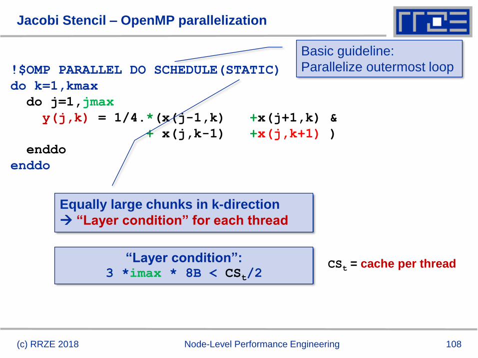
Jacobi Stencil – OpenMP parallelization
!$OMP PARALLEL DO SCHEDULE(STATIC)
do k=1,kmax
do j=1,jmax
y(j,k) = 1/4.*(x(j-1,k) +x(j+1,k) &
+ x(j,k-1) +x(j,k+1) )
enddo
enddo
“Layer condition”: 3 *imax * 8B < CSt/2
Basic guideline:
Parallelize outermost loop
Equally large chunks in k-direction
“Layer condition” for each thread
(c) RRZE 2018 Node-Level Performance Engineering
CSt = cache per thread
109
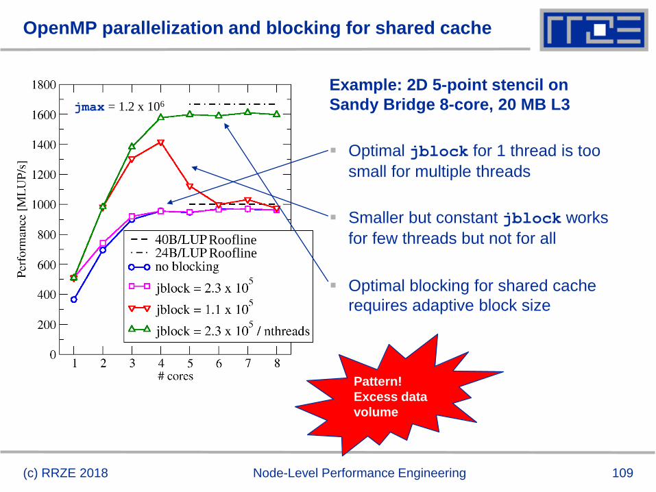
OpenMP parallelization and blocking for shared cache
(c) RRZE 2018 Node-Level Performance Engineering
Example: 2D 5-point stencil on
Sandy Bridge 8-core, 20 MB L3
Optimal jblock for 1 thread is too
small for multiple threads
Smaller but constant jblock works
for few threads but not for all
Optimal blocking for shared cache
requires adaptive block size
jmax = 1.2 x 10⁶
RooflineRoofline
Pattern!
Excess data
volume
112
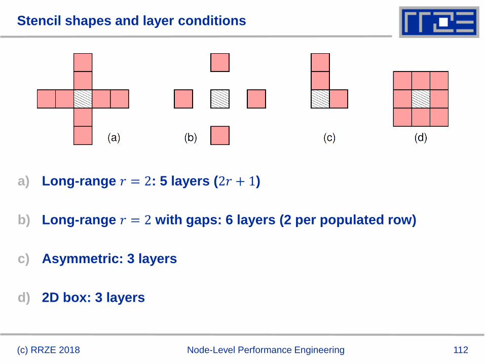
Stencil shapes and layer conditions
a) Long-range 𝑟 = 2: 5 layers (2𝑟 + 1)
b) Long-range 𝑟 = 2 with gaps: 6 layers (2 per populated row)
c) Asymmetric: 3 layers
d) 2D box: 3 layers
(c) RRZE 2018 Node-Level Performance Engineering
113
Conclusions from the Jacobi example
We have made sense of the memory-bound performance vs.
problem size
“Layer conditions” lead to predictions of code balance
“What part of the data comes from where” is a crucial question
The model works only if the bandwidth is “saturated”
In-cache modeling is more involved
Avoiding slow data paths == re-establishing the most favorable
layer condition
Improved code showed the speedup predicted by the model
Optimal blocking factor can be estimated
Be guided by the cache size the layer condition
No need for exhaustive scan of “optimization space”
Food for thought
Multi-dimensional loop blocking – would it make sense?
Can we choose a “better” OpenMP loop schedule?
What would change if we parallelized inner loops?
(c) RRZE 2018 Node-Level Performance Engineering
114
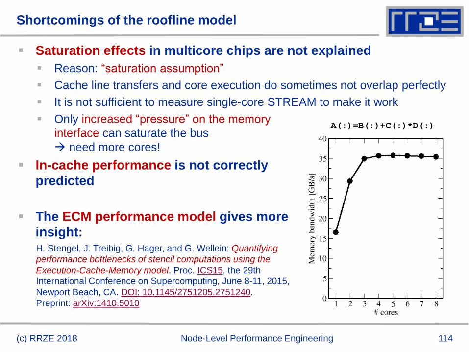
Shortcomings of the roofline model
Saturation effects in multicore chips are not explained
Reason: “saturation assumption”
Cache line transfers and core execution do sometimes not overlap perfectly
It is not sufficient to measure single-core STREAM to make it work
Only increased “pressure” on the memory
interface can saturate the bus
need more cores!
In-cache performance is not correctly
predicted
The ECM performance model gives more
insight:
A(:)=B(:)+C(:)*D(:)
(c) RRZE 2018 Node-Level Performance Engineering
H. Stengel, J. Treibig, G. Hager, and G. Wellein: Quantifying
performance bottlenecks of stencil computations using the
Execution-Cache-Memory model. Proc. ICS15, the 29th
International Conference on Supercomputing, June 8-11, 2015,
Newport Beach, CA. DOI: 10.1145/2751205.2751240.
Preprint: arXiv:1410.5010

Case study:
Sparse Matrix Vector Multiplication
116
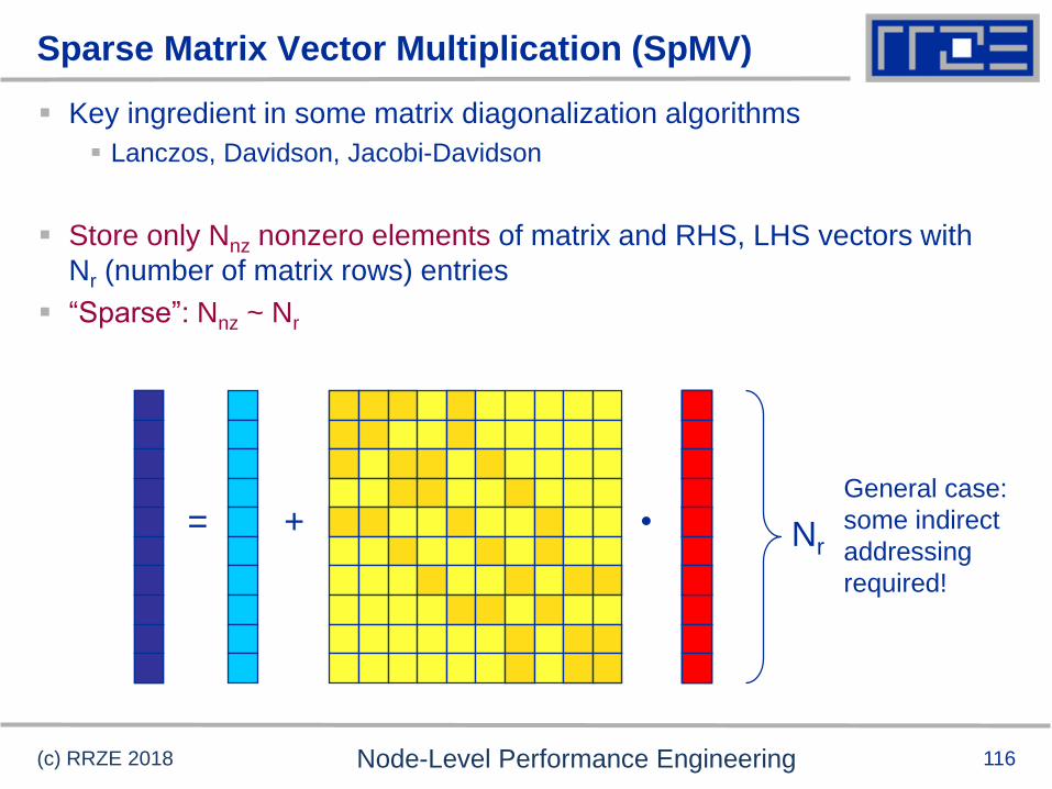
Sparse Matrix Vector Multiplication (SpMV)
Key ingredient in some matrix diagonalization algorithms
Lanczos, Davidson, Jacobi-Davidson
Store only Nnz nonzero elements of matrix and RHS, LHS vectors with
Nr (number of matrix rows) entries
“Sparse”: Nnz ~ Nr
(c) RRZE 2018 Node-Level Performance Engineering
= + • Nr
General case:
some indirect
addressing
required!
117
SpMVM characteristics
For large problems, SpMV is inevitably memory-bound
Intra-socket saturation effect on modern multicores
SpMV is easily parallelizable in shared and distributed memory
Load balancing
Communication overhead
Data storage format is crucial for performance properties
Most useful general format on CPUs:
Compressed Row Storage (CRS)
Depending on compute architecture
(c) RRZE 2018 Node-Level Performance Engineering
118
…
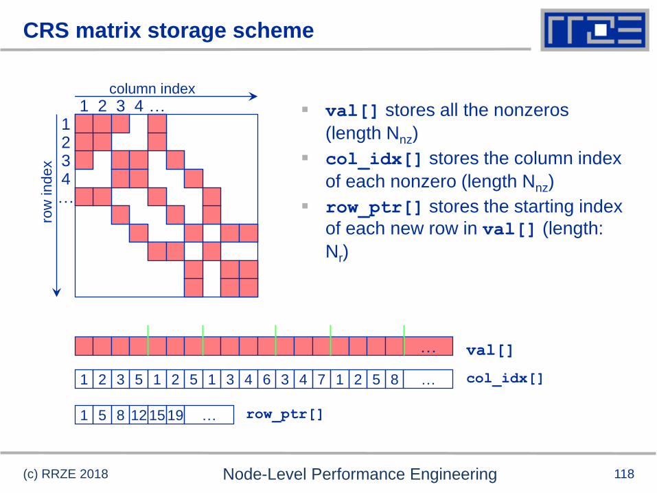
CRS matrix storage scheme
(c) RRZE 2018 Node-Level Performance Engineering
column index
row
index
1 2 3 4 …1234…
val[]
1 5 3 72 1 46323 4 21 5 815 … col_idx[]
1 5 15 198 12 … row_ptr[]
val[] stores all the nonzeros
(length Nnz)
col_idx[] stores the column index
of each nonzero (length Nnz)
row_ptr[] stores the starting index
of each new row in val[] (length:
Nr)
119(c) RRZE 2018 Node-Level Performance Engineering
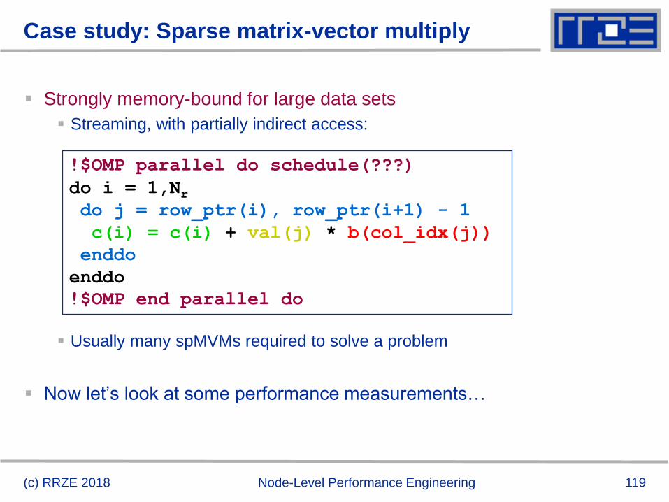
Case study: Sparse matrix-vector multiply
Strongly memory-bound for large data sets
Streaming, with partially indirect access:
Usually many spMVMs required to solve a problem
Now let’s look at some performance measurements…
do i = 1,Nrdo j = row_ptr(i), row_ptr(i+1) - 1
c(i) = c(i) + val(j) * b(col_idx(j))
enddo
enddo
!$OMP parallel do schedule(???)
!$OMP end parallel do
121
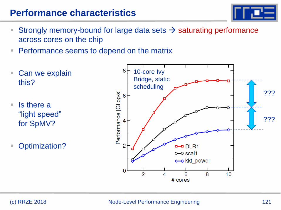
Performance characteristics
Strongly memory-bound for large data sets saturating performance
across cores on the chip
Performance seems to depend on the matrix
Can we explain
this?
Is there a
“light speed”
for SpMV?
Optimization?
(c) RRZE 2018 Node-Level Performance Engineering
???
???
10-core Ivy
Bridge, static
scheduling
122
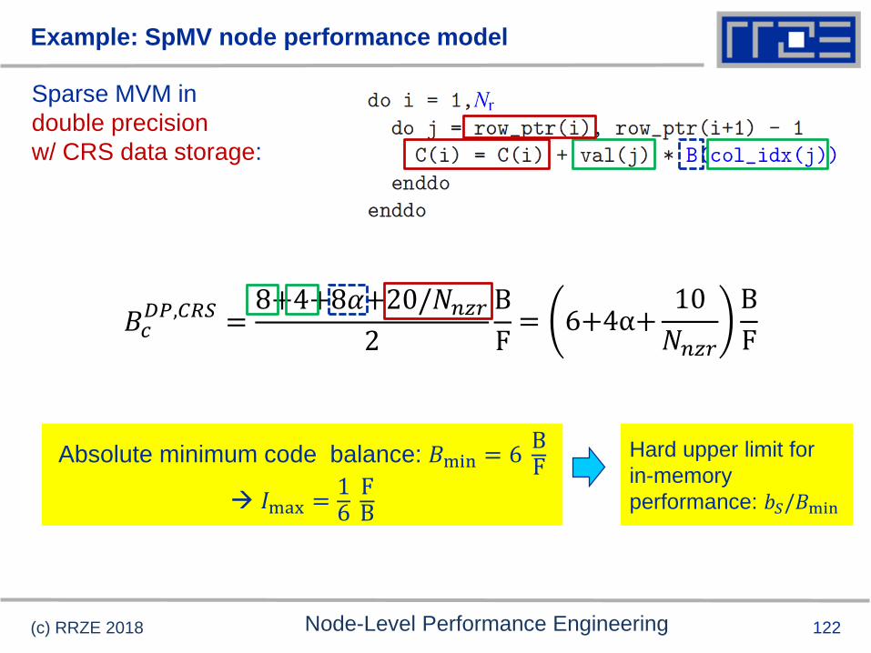
Example: SpMV node performance model
Sparse MVM in
double precision
w/ CRS data storage:
(c) RRZE 2018 Node-Level Performance Engineering
𝐵𝑐𝐷𝑃,𝐶𝑅𝑆 =
8+4+8𝛼+20/𝑁𝑛𝑧𝑟2
B
F
Absolute minimum code balance: 𝐵min = 6BF
𝐼max =16FB
= 6+4α+10
𝑁𝑛𝑧𝑟
B
F
Hard upper limit for
in-memory
performance: 𝑏𝑆/𝐵min
123
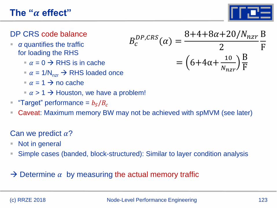
The “𝜶 effect”
DP CRS code balance
α quantifies the traffic
for loading the RHS
𝛼 = 0 RHS is in cache
𝛼 = 1/Nnzr RHS loaded once
𝛼 = 1 no cache
𝛼 > 1 Houston, we have a problem!
“Target” performance = 𝑏𝑆/𝐵𝑐 Caveat: Maximum memory BW may not be achieved with spMVM (see later)
Can we predict 𝛼?
Not in general
Simple cases (banded, block-structured): Similar to layer condition analysis
Determine 𝛼 by measuring the actual memory traffic
(c) RRZE 2018 Node-Level Performance Engineering
𝐵𝑐𝐷𝑃,𝐶𝑅𝑆(𝛼) =
8+4+8𝛼+20/𝑁𝑛𝑧𝑟2
B
F
= 6+4α+10
𝑁𝑛𝑧𝑟
BF
124
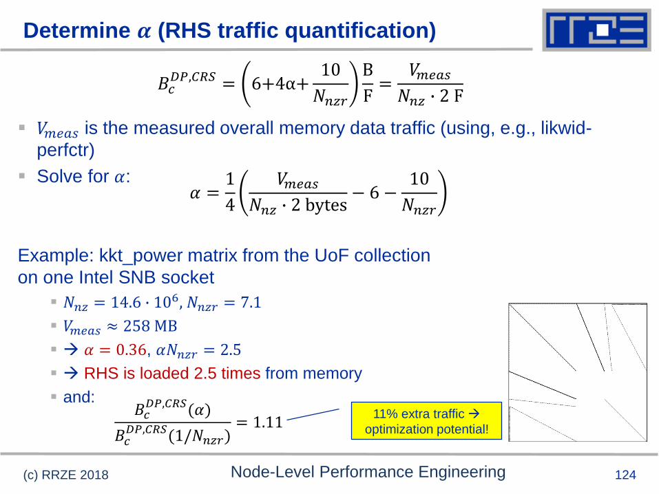
Determine 𝜶 (RHS traffic quantification)
𝑉𝑚𝑒𝑎𝑠 is the measured overall memory data traffic (using, e.g., likwid-
perfctr)
Solve for 𝛼:
Example: kkt_power matrix from the UoF collection
on one Intel SNB socket
𝑁𝑛𝑧 = 14.6 ∙ 106, 𝑁𝑛𝑧𝑟 = 7.1
𝑉𝑚𝑒𝑎𝑠 ≈ 258 MB
𝛼 = 0.36, 𝛼𝑁𝑛𝑧𝑟 = 2.5
RHS is loaded 2.5 times from memory
and:
(c) RRZE 2018 Node-Level Performance Engineering
𝐵𝑐𝐷𝑃,𝐶𝑅𝑆 = 6+4α+
10
𝑁𝑛𝑧𝑟
B
F=
𝑉𝑚𝑒𝑎𝑠
𝑁𝑛𝑧 ∙ 2 F
𝛼 =1
4
𝑉𝑚𝑒𝑎𝑠
𝑁𝑛𝑧 ∙ 2 bytes− 6 −
10
𝑁𝑛𝑧𝑟
𝐵𝑐𝐷𝑃,𝐶𝑅𝑆(𝛼)
𝐵𝑐𝐷𝑃,𝐶𝑅𝑆(1/𝑁𝑛𝑧𝑟)
= 1.1111% extra traffic
optimization potential!
125
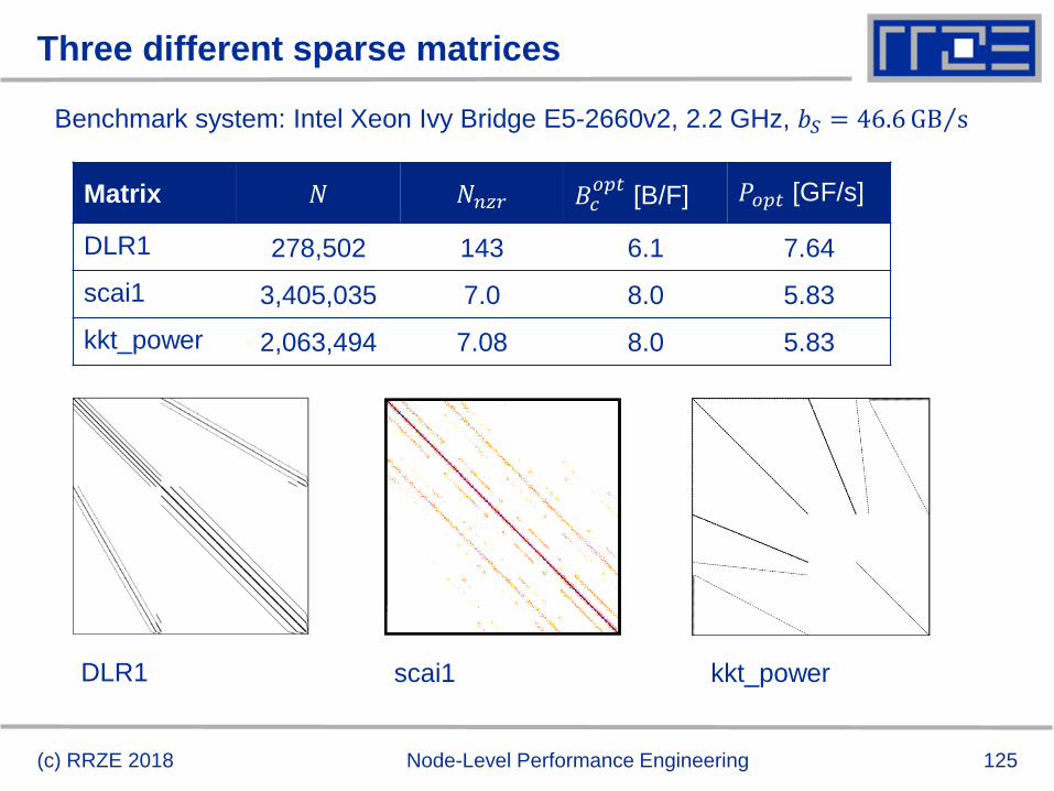
Three different sparse matrices
Matrix 𝑁 𝑁𝑛𝑧𝑟 𝐵𝑐𝑜𝑝𝑡
[B/F] 𝑃𝑜𝑝𝑡 [GF/s]
DLR1 278,502 143 6.1 7.64
scai1 3,405,035 7.0 8.0 5.83
kkt_power 2,063,494 7.08 8.0 5.83
(c) RRZE 2018 Node-Level Performance Engineering
DLR1 scai1 kkt_power
Benchmark system: Intel Xeon Ivy Bridge E5-2660v2, 2.2 GHz, 𝑏𝑆 = 46.6 ΤGB s
126
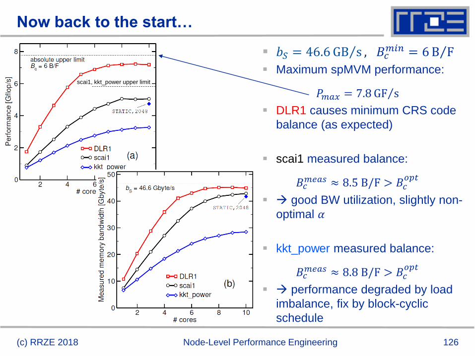
Now back to the start…
(c) RRZE 2018 Node-Level Performance Engineering
𝑏𝑆 = 46.6 ΤGB s , 𝐵𝑐𝑚𝑖𝑛 = 6 ΤB F
Maximum spMVM performance:
𝑃𝑚𝑎𝑥 = 7.8 ΤGF s
DLR1 causes minimum CRS code
balance (as expected)
scai1 measured balance:
𝐵𝑐𝑚𝑒𝑎𝑠 ≈ 8.5 B/F > 𝐵𝑐
𝑜𝑝𝑡
good BW utilization, slightly non-
optimal 𝛼
kkt_power measured balance:
𝐵𝑐𝑚𝑒𝑎𝑠 ≈ 8.8 B/F > 𝐵𝑐
𝑜𝑝𝑡
performance degraded by load
imbalance, fix by block-cyclic
schedule
scai1, kkt_power upper limit
127
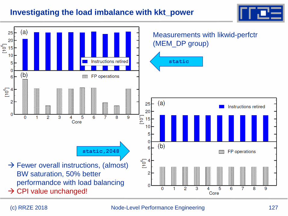
Investigating the load imbalance with kkt_power
(c) RRZE 2018 Node-Level Performance Engineering
static,2048
static
Fewer overall instructions, (almost)
BW saturation, 50% better
performandce with load balancing
CPI value unchanged!
Measurements with likwid-perfctr
(MEM_DP group)
128
Roofline analysis for spMVM
Conclusion from the Roofline analysis
The roofline model does not “work” for spMVM due to the RHS
traffic uncertainties
We have “turned the model around” and measured the actual
memory traffic to determine the RHS overhead
Result indicates:
1. how much actual traffic the RHS generates
2. how efficient the RHS access is (compare BW with max. BW)
3. how much optimization potential we have with matrix reordering
Do not forget about load balancing!
Consequence: Modeling is not always 100% predictive. It‘s all about
learning more about performance properties!
(c) RRZE 2018 Node-Level Performance Engineering
Case study:
Tall & Skinny Matrix-Transpose Times
Tall & Skinny Matrix (TSMTTSM)
Multiplication

130
TSMTTSM Multiplication
Block of vectors Tall & Skinny Matrix (e.g. 107 x 101 dense matrix)
Row-major storage format (see SpMVM)
Block vector subspace orthogonalization procedure requires, e.g.
computation of scalar product between vectors of two blocks
TSMTTSM Mutliplication
𝐾 ≫ 𝑁,𝑀
Assume: 𝛼 = 1; 𝛽 = 0
(c) RRZE 2018 Node-Level Performance Engineering
M
N K
131
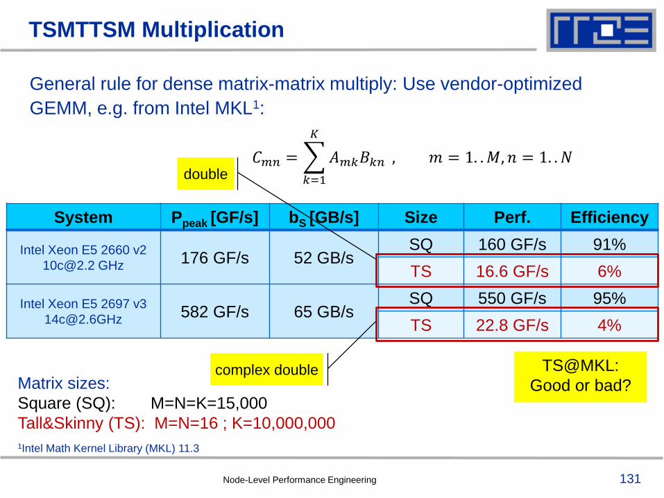
General rule for dense matrix-matrix multiply: Use vendor-optimized
GEMM, e.g. from Intel MKL1:
TSMTTSM Multiplication
Node-Level Performance Engineering
System Ppeak [GF/s] bS [GB/s] Size Perf. Efficiency
Intel Xeon E5 2660 v2
[email protected] GHz176 GF/s 52 GB/s
SQ 160 GF/s 91%
TS 16.6 GF/s 6%
Intel Xeon E5 2697 v3
[email protected] GF/s 65 GB/s
SQ 550 GF/s 95%
TS 22.8 GF/s 4%
Matrix sizes:
Square (SQ): M=N=K=15,000
Tall&Skinny (TS): M=N=16 ; K=10,000,000
1Intel Math Kernel Library (MKL) 11.3
complex double
double
TS@MKL:
Good or bad?
𝐶𝑚𝑛 =
𝑘=1
𝐾
𝐴𝑚𝑘𝐵𝑘𝑛 , 𝑚 = 1. .𝑀, 𝑛 = 1. . 𝑁
132
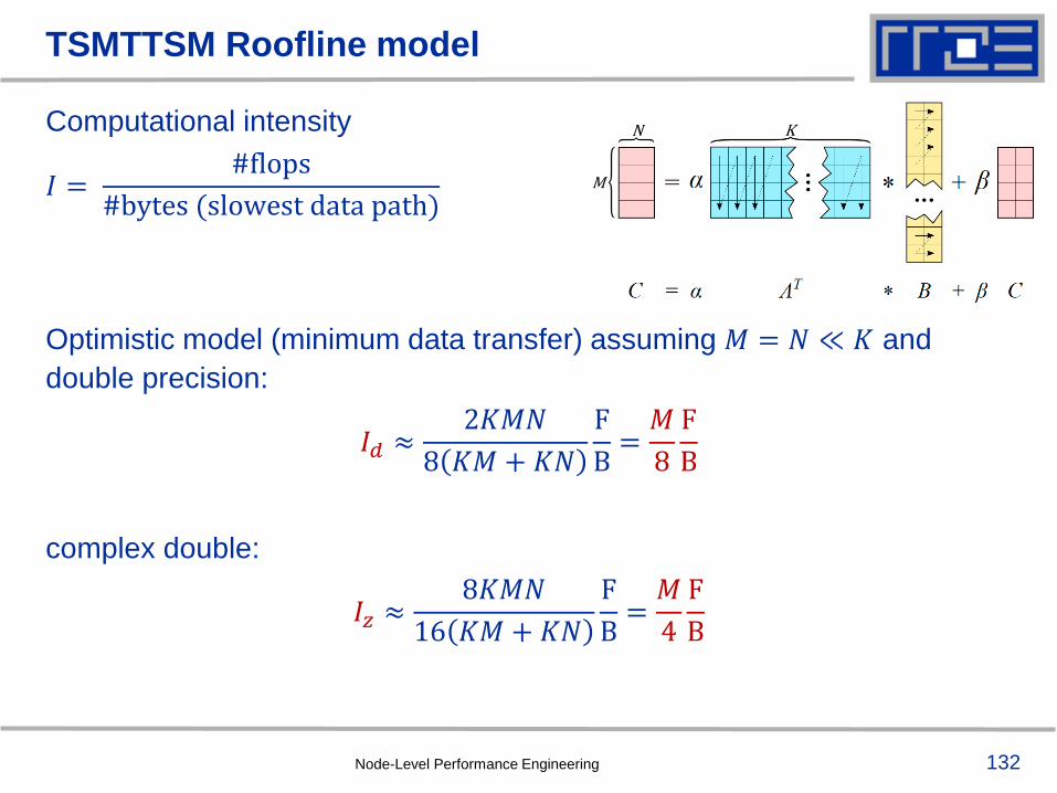
M
N KComputational intensity
𝐼 =#flops
#bytes (slowest data path)
Optimistic model (minimum data transfer) assuming 𝑀 = 𝑁 ≪ 𝐾 and
double precision:
𝐼𝑑 ≈2𝐾𝑀𝑁
8 𝐾𝑀 + 𝐾𝑁
F
B=𝑀
8
F
B
complex double:
𝐼𝑧 ≈8𝐾𝑀𝑁
16 𝐾𝑀 + 𝐾𝑁
F
B=𝑀
4
F
B
TSMTTSM Roofline model
Node-Level Performance Engineering
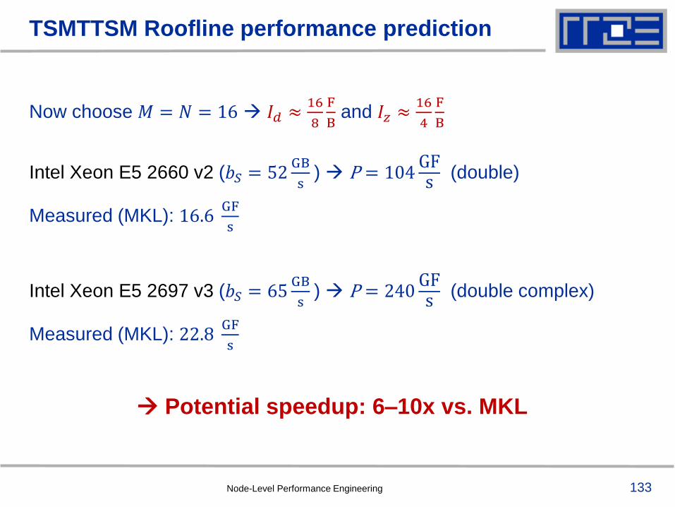
133
Now choose 𝑀 = 𝑁 = 16 𝐼𝑑 ≈16
8
F
Band 𝐼𝑧 ≈
16
4
F
B
Intel Xeon E5 2660 v2 (𝑏𝑆 = 52GB
s) P = 104
GFs
(double)
Measured (MKL): 16.6GF
s
Intel Xeon E5 2697 v3 (𝑏𝑆 = 65GB
s) P = 240
GFs
(double complex)
Measured (MKL): 22.8GF
s
TSMTTSM Roofline performance prediction
Potential speedup: 6–10x vs. MKL
Node-Level Performance Engineering
134
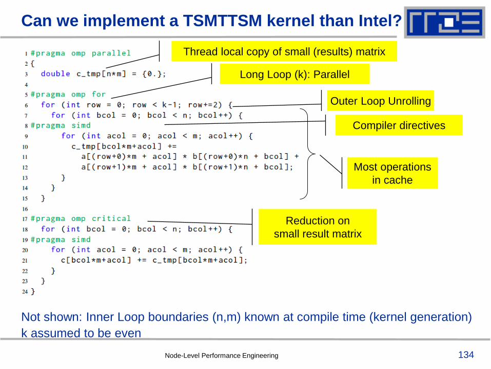
Not shown: Inner Loop boundaries (n,m) known at compile time (kernel generation)
k assumed to be even
Can we implement a TSMTTSM kernel than Intel?
Long Loop (k): Parallel
Outer Loop Unrolling
Compiler directives
Most operations
in cache
Reduction on
small result matrix
Node-Level Performance Engineering
Thread local copy of small (results) matrix
135
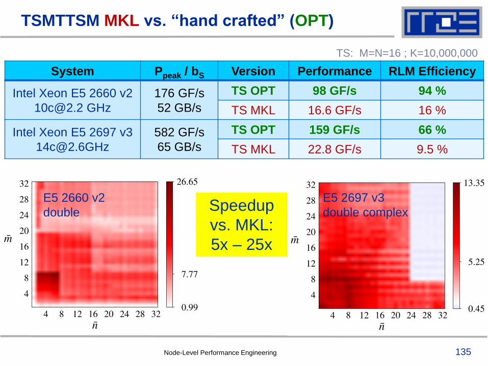
TSMTTSM MKL vs. “hand crafted” (OPT)
System Ppeak / bS Version Performance RLM Efficiency
Intel Xeon E5 2660 v2
176 GF/s
52 GB/s
TS OPT 98 GF/s 94 %
TS MKL 16.6 GF/s 16 %
Intel Xeon E5 2697 v3
582 GF/s
65 GB/s
TS OPT 159 GF/s 66 %
TS MKL 22.8 GF/s 9.5 %
TS: M=N=16 ; K=10,000,000
E5 2660 v2
double
E5 2697 v3
double complexSpeedup
vs. MKL:
5x – 25x
Node-Level Performance Engineering

ERLANGEN REGIONAL
COMPUTING CENTER
Single Instruction Multiple Data
(SIMD)
137
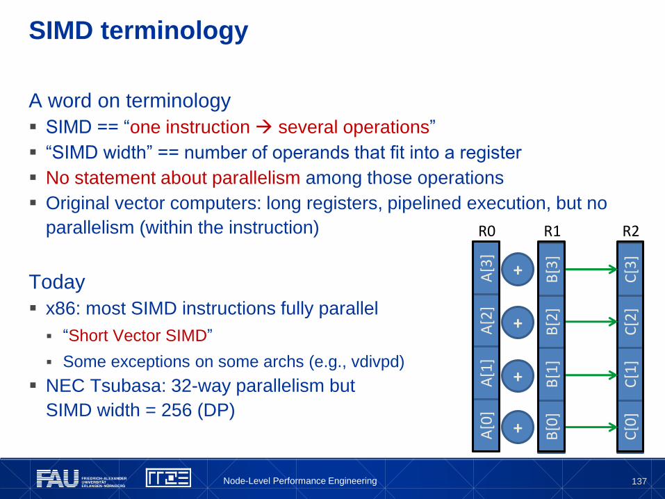
A word on terminology
SIMD == “one instruction several operations”
“SIMD width” == number of operands that fit into a register
No statement about parallelism among those operations
Original vector computers: long registers, pipelined execution, but no
parallelism (within the instruction)
Today
x86: most SIMD instructions fully parallel
“Short Vector SIMD”
Some exceptions on some archs (e.g., vdivpd)
NEC Tsubasa: 32-way parallelism but
SIMD width = 256 (DP)
SIMD terminology
A[0
]A
[1]
A[2
]A
[3]
B[0
]B
[1]
B[2
]B
[3]
C[0
]C
[1]
C[2
]C
[3]
+
+
+
+
R0 R1 R2
Node-Level Performance Engineering
138
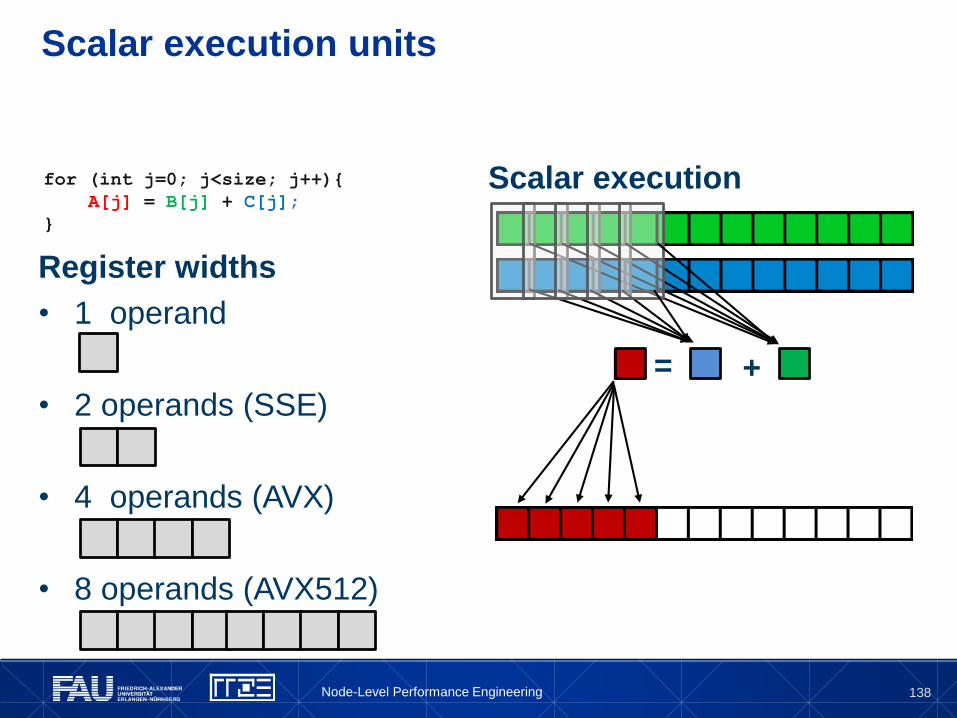
Scalar execution units
for (int j=0; j<size; j++){
A[j] = B[j] + C[j];
}
Scalar execution
Register widths
• 1 operand
• 2 operands (SSE)
• 4 operands (AVX)
• 8 operands (AVX512)
= +
Node-Level Performance Engineering
139
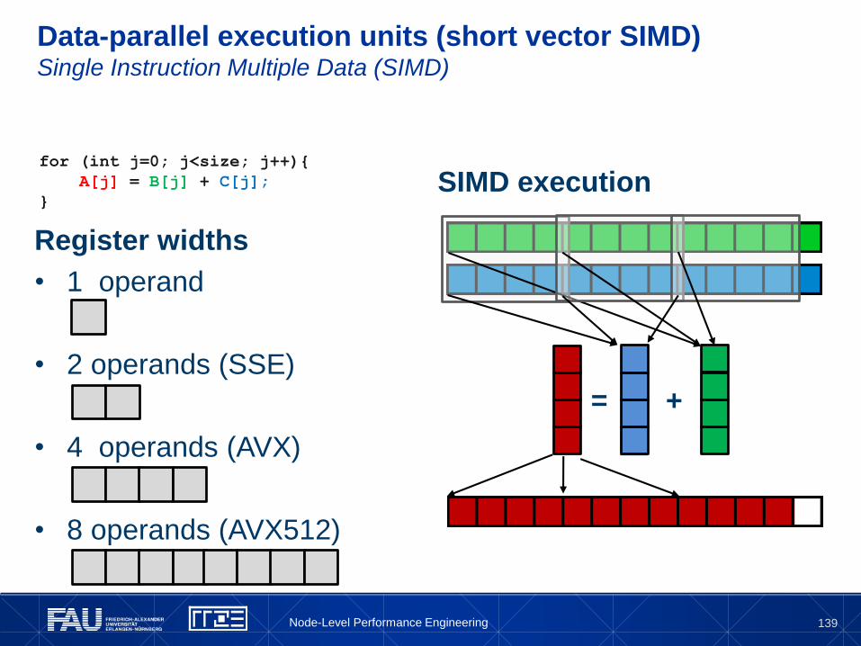
Data-parallel execution units (short vector SIMD)Single Instruction Multiple Data (SIMD)
for (int j=0; j<size; j++){
A[j] = B[j] + C[j];
}
Register widths
• 1 operand
• 2 operands (SSE)
• 4 operands (AVX)
• 8 operands (AVX512)
SIMD execution
= +
Node-Level Performance Engineering
140
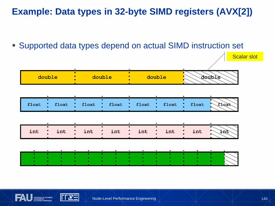
Example: Data types in 32-byte SIMD registers (AVX[2])
Supported data types depend on actual SIMD instruction set
Scalar slot
Node-Level Performance Engineering
141
In-core features are driving peak performance
SSE2
AVX
AVX512
FMA
Node-Level Performance Engineering
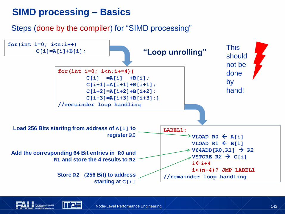
142
SIMD processing – Basics
Steps (done by the compiler) for “SIMD processing”
for(int i=0; i<n;i++)
C[i]=A[i]+B[i];
for(int i=0; i<n;i+=4){
C[i] =A[i] +B[i];
C[i+1]=A[i+1]+B[i+1];
C[i+2]=A[i+2]+B[i+2];
C[i+3]=A[i+3]+B[i+3];}
//remainder loop handling
LABEL1:
VLOAD R0 A[i]
VLOAD R1 B[i]
V64ADD[R0,R1] R2
VSTORE R2 C[i]
ii+4
i<(n-4)? JMP LABEL1
//remainder loop handling
“Loop unrolling”
Load 256 Bits starting from address of A[i] to
register R0
Add the corresponding 64 Bit entries in R0 and
R1 and store the 4 results to R2
Store R2 (256 Bit) to address
starting at C[i]
This
should
not be
done
by
hand!
Node-Level Performance Engineering
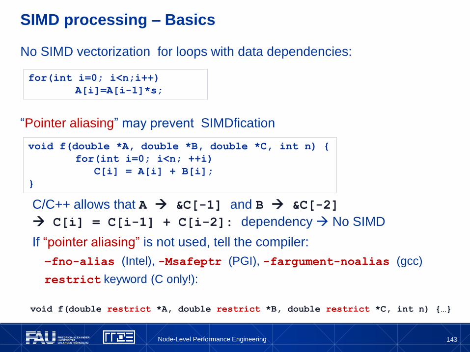
143
SIMD processing – Basics
No SIMD vectorization for loops with data dependencies:
“Pointer aliasing” may prevent SIMDfication
C/C++ allows that A &C[-1] and B &C[-2]
C[i] = C[i-1] + C[i-2]: dependency No SIMD
If “pointer aliasing” is not used, tell the compiler:
–fno-alias (Intel), -Msafeptr (PGI), -fargument-noalias (gcc)
restrict keyword (C only!):
for(int i=0; i<n;i++)
A[i]=A[i-1]*s;
void f(double *A, double *B, double *C, int n) {
for(int i=0; i<n; ++i)
C[i] = A[i] + B[i];
}
void f(double restrict *A, double restrict *B, double restrict *C, int n) {…}
Node-Level Performance Engineering
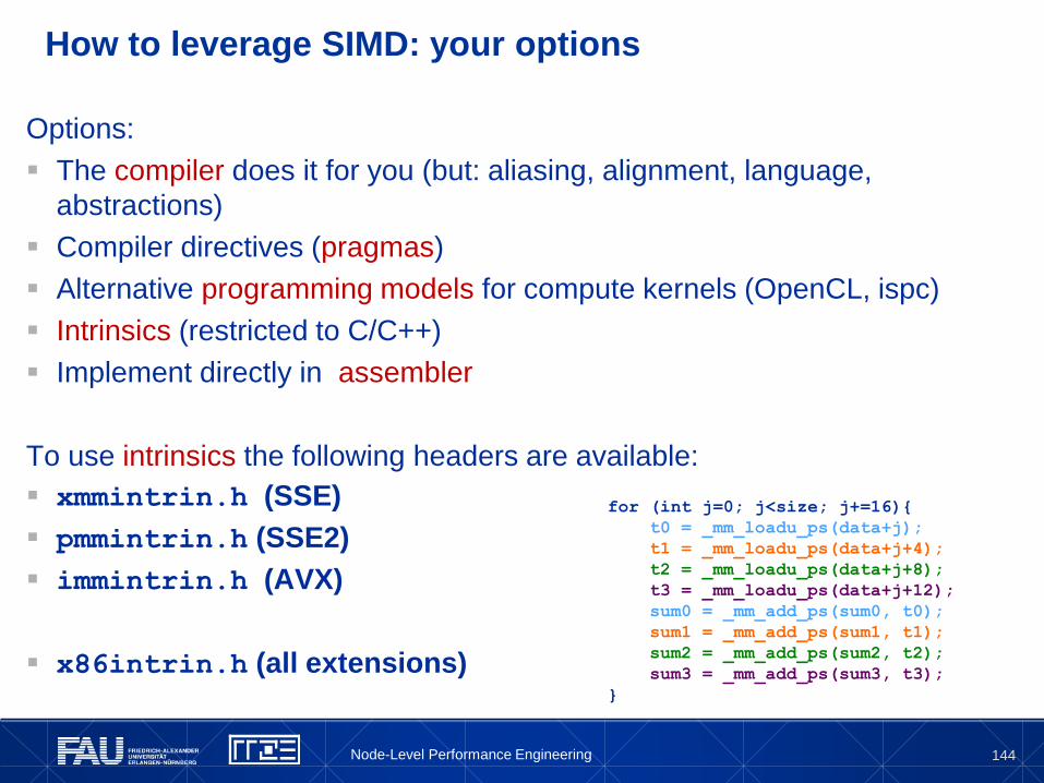
144
Options:
The compiler does it for you (but: aliasing, alignment, language,
abstractions)
Compiler directives (pragmas)
Alternative programming models for compute kernels (OpenCL, ispc)
Intrinsics (restricted to C/C++)
Implement directly in assembler
To use intrinsics the following headers are available:
xmmintrin.h (SSE)
pmmintrin.h (SSE2)
immintrin.h (AVX)
x86intrin.h (all extensions)
How to leverage SIMD: your options
for (int j=0; j<size; j+=16){
t0 = _mm_loadu_ps(data+j);
t1 = _mm_loadu_ps(data+j+4);
t2 = _mm_loadu_ps(data+j+8);
t3 = _mm_loadu_ps(data+j+12);
sum0 = _mm_add_ps(sum0, t0);
sum1 = _mm_add_ps(sum1, t1);
sum2 = _mm_add_ps(sum2, t2);
sum3 = _mm_add_ps(sum3, t3);
}
Node-Level Performance Engineering
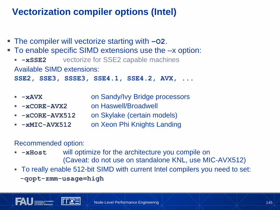
145
Vectorization compiler options (Intel)
The compiler will vectorize starting with –O2. To enable specific SIMD extensions use the –x option:
-xSSE2 vectorize for SSE2 capable machines
Available SIMD extensions:
SSE2, SSE3, SSSE3, SSE4.1, SSE4.2, AVX, ...
-xAVX on Sandy/Ivy Bridge processors
-xCORE-AVX2 on Haswell/Broadwell
-xCORE-AVX512 on Skylake (certain models)
-xMIC-AVX512 on Xeon Phi Knights Landing
Recommended option:
-xHost will optimize for the architecture you compile on(Caveat: do not use on standalone KNL, use MIC-AVX512)
To really enable 512-bit SIMD with current Intel compilers you need to set:
-qopt-zmm-usage=high
Node-Level Performance Engineering
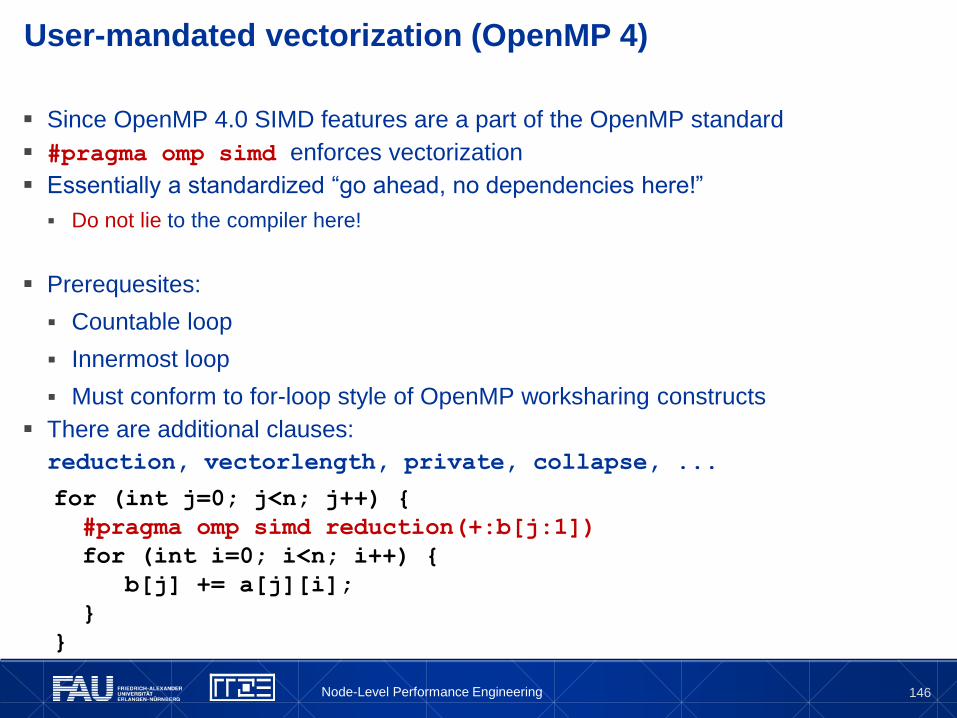
146
User-mandated vectorization (OpenMP 4)
Since OpenMP 4.0 SIMD features are a part of the OpenMP standard
#pragma omp simd enforces vectorization
Essentially a standardized “go ahead, no dependencies here!”
Do not lie to the compiler here!
Prerequesites:
Countable loop
Innermost loop
Must conform to for-loop style of OpenMP worksharing constructs
There are additional clauses:
reduction, vectorlength, private, collapse, ...
for (int j=0; j<n; j++) {
#pragma omp simd reduction(+:b[j:1])
for (int i=0; i<n; i++) {
b[j] += a[j][i];
}
}
Node-Level Performance Engineering
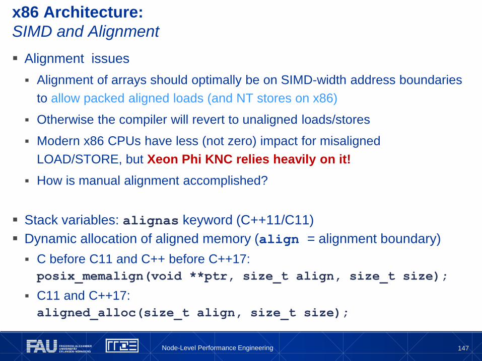
147
x86 Architecture:
SIMD and Alignment
Alignment issues
Alignment of arrays should optimally be on SIMD-width address boundaries
to allow packed aligned loads (and NT stores on x86)
Otherwise the compiler will revert to unaligned loads/stores
Modern x86 CPUs have less (not zero) impact for misaligned
LOAD/STORE, but Xeon Phi KNC relies heavily on it!
How is manual alignment accomplished?
Stack variables: alignas keyword (C++11/C11)
Dynamic allocation of aligned memory (align = alignment boundary)
C before C11 and C++ before C++17:
posix_memalign(void **ptr, size_t align, size_t size);
C11 and C++17:
aligned_alloc(size_t align, size_t size);
Node-Level Performance Engineering
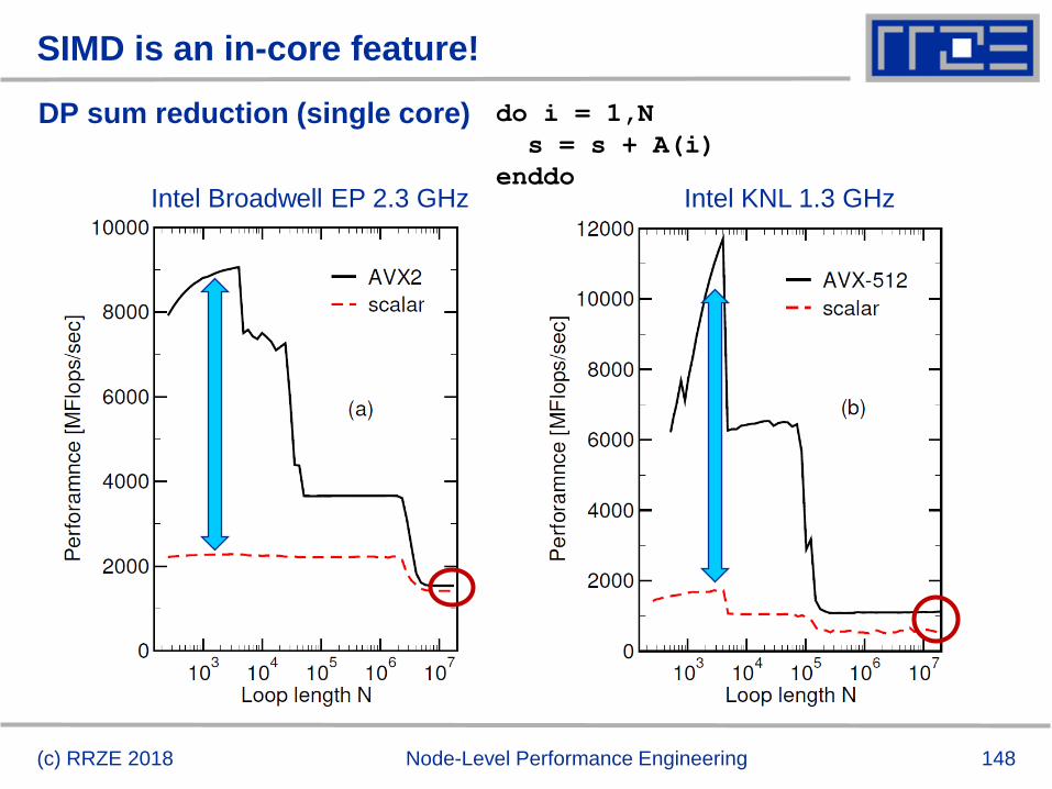
148
SIMD is an in-core feature!
DP sum reduction (single core)
(c) RRZE 2018 Node-Level Performance Engineering
Intel Broadwell EP 2.3 GHz Intel KNL 1.3 GHz
do i = 1,N
s = s + A(i)
enddo
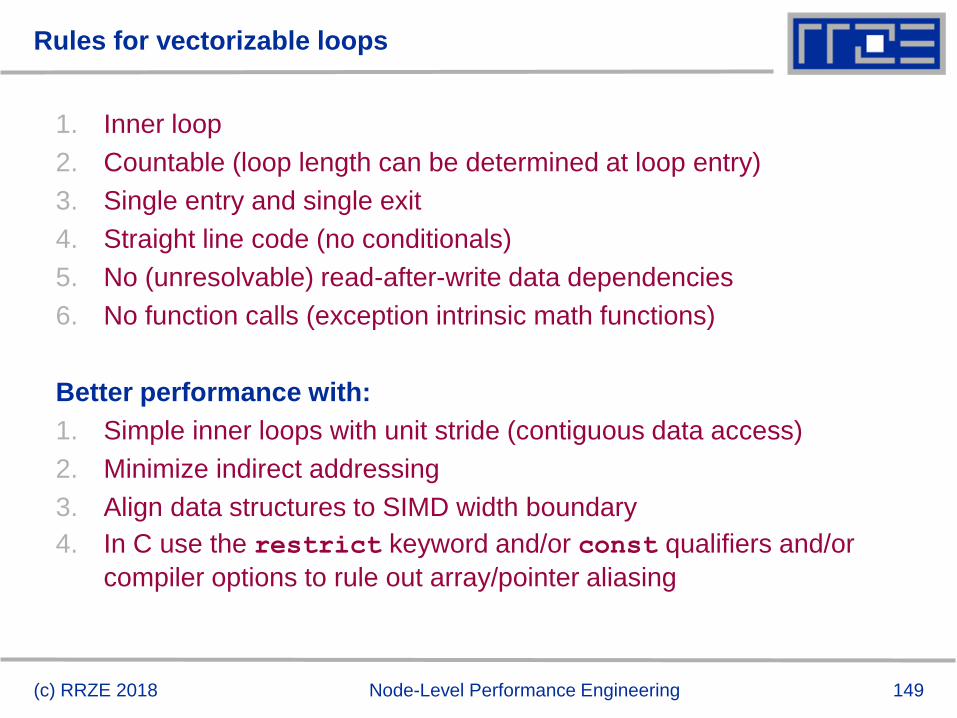
149(c) RRZE 2018 Node-Level Performance Engineering
Rules for vectorizable loops
1. Inner loop
2. Countable (loop length can be determined at loop entry)
3. Single entry and single exit
4. Straight line code (no conditionals)
5. No (unresolvable) read-after-write data dependencies
6. No function calls (exception intrinsic math functions)
Better performance with:
1. Simple inner loops with unit stride (contiguous data access)
2. Minimize indirect addressing
3. Align data structures to SIMD width boundary
4. In C use the restrict keyword and/or const qualifiers and/or
compiler options to rule out array/pointer aliasing
Efficient parallel programming
on ccNUMA nodes
Performance characteristics of ccNUMA nodes
First touch placement policy
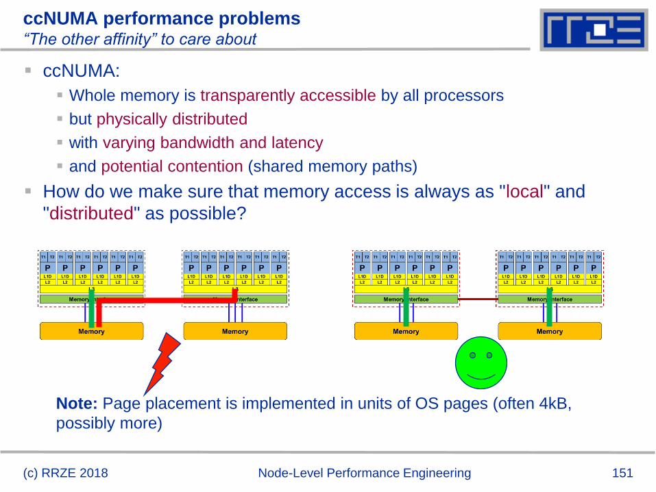
151(c) RRZE 2018 Node-Level Performance Engineering
ccNUMA performance problems“The other affinity” to care about
ccNUMA:
Whole memory is transparently accessible by all processors
but physically distributed
with varying bandwidth and latency
and potential contention (shared memory paths)
How do we make sure that memory access is always as "local" and
"distributed" as possible?
Note: Page placement is implemented in units of OS pages (often 4kB,
possibly more)
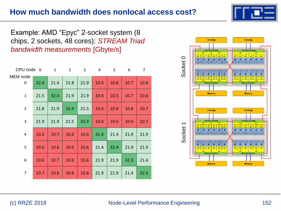
152
How much bandwidth does nonlocal access cost?
(c) RRZE 2018 Node-Level Performance Engineering
Example: AMD “Epyc” 2-socket system (8
chips, 2 sockets, 48 cores): STREAM Triad
bandwidth measurements [Gbyte/s]
So
cke
t 0
So
cke
t 1
0 1 2 3 4 5 6 7
0 32.4 21.4 21.8 21.9 10.6 10.6 10.7 10.8
1 21.5 32.4 21.9 21.9 10.6 10.5 10.7 10.6
2 21.8 21.9 32.4 21.5 10.6 10.6 10.8 10.7
3 21.9 21.9 21.5 32.4 10.6 10.6 10.6 10.7
4 10.6 10.7 10.6 10.6 32.4 21.4 21.9 21.9
5 10.6 10.6 10.6 10.6 21.4 32.4 21.9 21.9
6 10.6 10.7 10.6 10.6 21.9 21.9 32.3 21.4
7 10.7 10.6 10.6 10.6 21.9 21.9 21.4 32.5
CPU node
MEM node
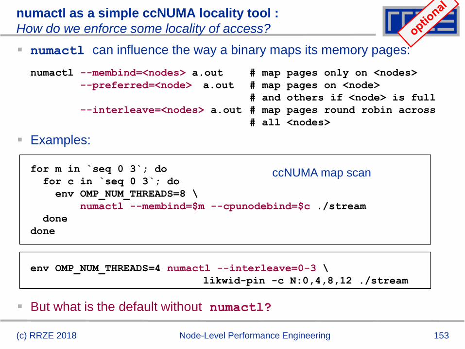
153(c) RRZE 2018 Node-Level Performance Engineering
numactl as a simple ccNUMA locality tool :
How do we enforce some locality of access?
numactl can influence the way a binary maps its memory pages:
numactl --membind=<nodes> a.out # map pages only on <nodes>
--preferred=<node> a.out # map pages on <node>
# and others if <node> is full
--interleave=<nodes> a.out # map pages round robin across
# all <nodes>
Examples:
for m in `seq 0 3`; do
for c in `seq 0 3`; do
env OMP_NUM_THREADS=8 \
numactl --membind=$m --cpunodebind=$c ./stream
done
done
env OMP_NUM_THREADS=4 numactl --interleave=0-3 \
likwid-pin -c N:0,4,8,12 ./stream
But what is the default without numactl?
ccNUMA map scan
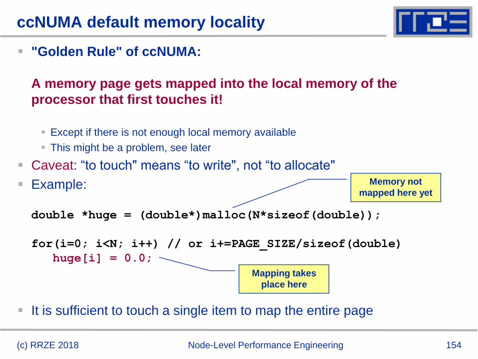
154(c) RRZE 2018 Node-Level Performance Engineering
ccNUMA default memory locality
"Golden Rule" of ccNUMA:
A memory page gets mapped into the local memory of the
processor that first touches it!
Except if there is not enough local memory available
This might be a problem, see later
Caveat: “to touch" means “to write", not “to allocate"
Example:
double *huge = (double*)malloc(N*sizeof(double));
for(i=0; i<N; i++) // or i+=PAGE_SIZE/sizeof(double)
huge[i] = 0.0;
It is sufficient to touch a single item to map the entire page
Memory not
mapped here yet
Mapping takes
place here
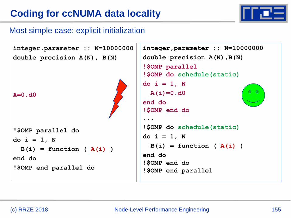
155(c) RRZE 2018 Node-Level Performance Engineering
Coding for ccNUMA data locality
integer,parameter :: N=10000000
double precision A(N), B(N)
A=0.d0
!$OMP parallel do
do i = 1, N
B(i) = function ( A(i) )
end do
!$OMP end parallel do
integer,parameter :: N=10000000
double precision A(N),B(N)
!$OMP parallel
!$OMP do schedule(static)
do i = 1, N
A(i)=0.d0
end do
!$OMP end do
...
!$OMP do schedule(static)
do i = 1, N
B(i) = function ( A(i) )
end do
!$OMP end do
!$OMP end parallel
Most simple case: explicit initialization
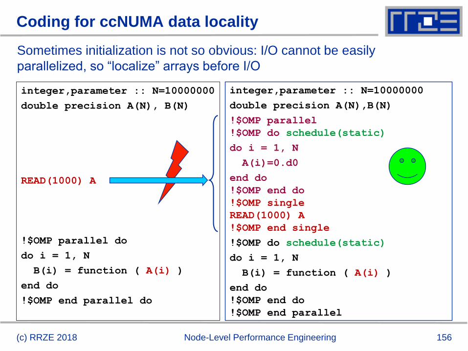
156(c) RRZE 2018 Node-Level Performance Engineering
Coding for ccNUMA data locality
integer,parameter :: N=10000000
double precision A(N), B(N)
READ(1000) A
!$OMP parallel do
do i = 1, N
B(i) = function ( A(i) )
end do
!$OMP end parallel do
integer,parameter :: N=10000000
double precision A(N),B(N)
!$OMP parallel
!$OMP do schedule(static)
do i = 1, N
A(i)=0.d0
end do
!$OMP end do
!$OMP single
READ(1000) A
!$OMP end single
!$OMP do schedule(static)
do i = 1, N
B(i) = function ( A(i) )
end do
!$OMP end do
!$OMP end parallel
Sometimes initialization is not so obvious: I/O cannot be easily
parallelized, so “localize” arrays before I/O
157(c) RRZE 2018 Node-Level Performance Engineering
Coding for Data Locality
Required condition: OpenMP loop schedule of initialization must be the
same as in all computational loops
Only choice: static! Specify explicitly on all NUMA-sensitive loops, just to
be sure…
Imposes some constraints on possible optimizations (e.g. load balancing)
Presupposes that all worksharing loops with the same loop length have the
same thread-chunk mapping
If dynamic scheduling/tasking is unavoidable, more advanced methods may
be in order
OpenMP 5.0 will have rudimentary memory affinity functionality
How about global objects?
Better not use them
If communication vs. computation is favorable, might consider properly
placed copies of global data
C++: Arrays of objects and std::vector<> are by default initialized
sequentially
STL allocators provide an elegant solution
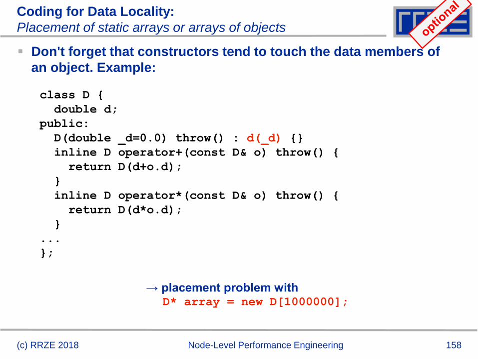
158(c) RRZE 2018 Node-Level Performance Engineering
Coding for Data Locality:
Placement of static arrays or arrays of objects
Don't forget that constructors tend to touch the data members of
an object. Example:
class D {
double d;
public:
D(double _d=0.0) throw() : d(_d) {}
inline D operator+(const D& o) throw() {
return D(d+o.d);
}
inline D operator*(const D& o) throw() {
return D(d*o.d);
}
...
};
→ placement problem with D* array = new D[1000000];
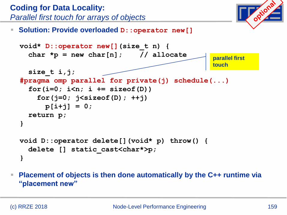
159(c) RRZE 2018 Node-Level Performance Engineering
Coding for Data Locality:
Parallel first touch for arrays of objects
Solution: Provide overloaded D::operator new[]
Placement of objects is then done automatically by the C++ runtime via
“placement new”
void* D::operator new[](size_t n) {
char *p = new char[n]; // allocate
size_t i,j;
#pragma omp parallel for private(j) schedule(...)
for(i=0; i<n; i += sizeof(D))
for(j=0; j<sizeof(D); ++j)
p[i+j] = 0;
return p;
}
void D::operator delete[](void* p) throw() {
delete [] static_cast<char*>p;
}
parallel first
touch
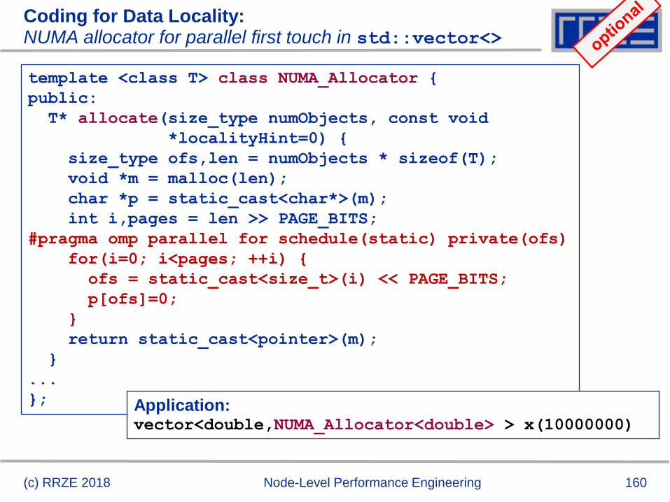
160(c) RRZE 2018 Node-Level Performance Engineering
Coding for Data Locality:NUMA allocator for parallel first touch in std::vector<>
template <class T> class NUMA_Allocator {
public:
T* allocate(size_type numObjects, const void
*localityHint=0) {
size_type ofs,len = numObjects * sizeof(T);
void *m = malloc(len);
char *p = static_cast<char*>(m);
int i,pages = len >> PAGE_BITS;
#pragma omp parallel for schedule(static) private(ofs)
for(i=0; i<pages; ++i) {
ofs = static_cast<size_t>(i) << PAGE_BITS;
p[ofs]=0;
}
return static_cast<pointer>(m);
}
...
}; Application:vector<double,NUMA_Allocator<double> > x(10000000)
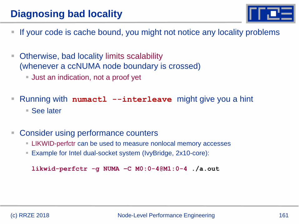
161(c) RRZE 2018 Node-Level Performance Engineering
Diagnosing bad locality
If your code is cache bound, you might not notice any locality problems
Otherwise, bad locality limits scalability
(whenever a ccNUMA node boundary is crossed)
Just an indication, not a proof yet
Running with numactl --interleave might give you a hint
See later
Consider using performance counters
LIKWID-perfctr can be used to measure nonlocal memory accesses
Example for Intel dual-socket system (IvyBridge, 2x10-core):
likwid-perfctr -g NUMA –C M0:0-4@M1:0-4 ./a.out
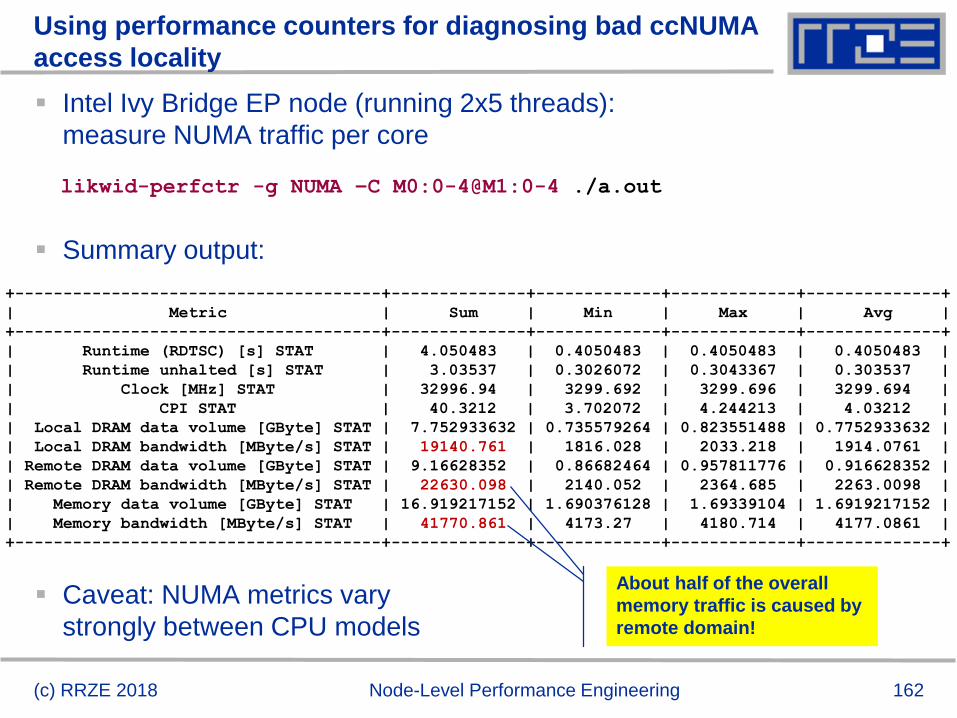
162(c) RRZE 2018 Node-Level Performance Engineering
Using performance counters for diagnosing bad ccNUMA
access locality
Intel Ivy Bridge EP node (running 2x5 threads):
measure NUMA traffic per core
Summary output:
Caveat: NUMA metrics vary
strongly between CPU models
+--------------------------------------+--------------+-------------+-------------+--------------+
| Metric | Sum | Min | Max | Avg |
+--------------------------------------+--------------+-------------+-------------+--------------+
| Runtime (RDTSC) [s] STAT | 4.050483 | 0.4050483 | 0.4050483 | 0.4050483 |
| Runtime unhalted [s] STAT | 3.03537 | 0.3026072 | 0.3043367 | 0.303537 |
| Clock [MHz] STAT | 32996.94 | 3299.692 | 3299.696 | 3299.694 |
| CPI STAT | 40.3212 | 3.702072 | 4.244213 | 4.03212 |
| Local DRAM data volume [GByte] STAT | 7.752933632 | 0.735579264 | 0.823551488 | 0.7752933632 |
| Local DRAM bandwidth [MByte/s] STAT | 19140.761 | 1816.028 | 2033.218 | 1914.0761 |
| Remote DRAM data volume [GByte] STAT | 9.16628352 | 0.86682464 | 0.957811776 | 0.916628352 |
| Remote DRAM bandwidth [MByte/s] STAT | 22630.098 | 2140.052 | 2364.685 | 2263.0098 |
| Memory data volume [GByte] STAT | 16.919217152 | 1.690376128 | 1.69339104 | 1.6919217152 |
| Memory bandwidth [MByte/s] STAT | 41770.861 | 4173.27 | 4180.714 | 4177.0861 |
+--------------------------------------+--------------+-------------+-------------+--------------+
likwid-perfctr -g NUMA –C M0:0-4@M1:0-4 ./a.out
About half of the overall
memory traffic is caused by
remote domain!
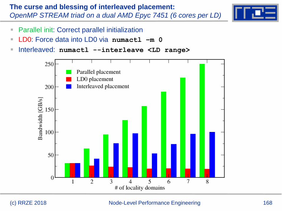
168
The curse and blessing of interleaved placement:
OpenMP STREAM triad on a dual AMD Epyc 7451 (6 cores per LD)
Parallel init: Correct parallel initialization
LD0: Force data into LD0 via numactl –m 0
Interleaved: numactl --interleave <LD range>
(c) RRZE 2018 Node-Level Performance Engineering
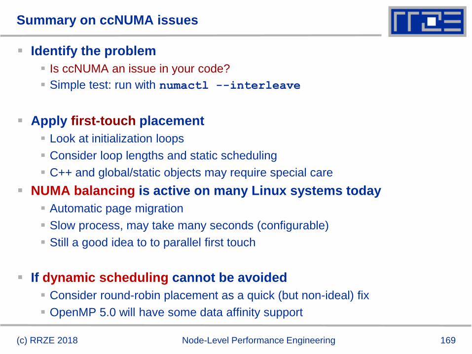
169
Summary on ccNUMA issues
Identify the problem
Is ccNUMA an issue in your code?
Simple test: run with numactl --interleave
Apply first-touch placement
Look at initialization loops
Consider loop lengths and static scheduling
C++ and global/static objects may require special care
NUMA balancing is active on many Linux systems today
Automatic page migration
Slow process, may take many seconds (configurable)
Still a good idea to to parallel first touch
If dynamic scheduling cannot be avoided
Consider round-robin placement as a quick (but non-ideal) fix
OpenMP 5.0 will have some data affinity support
(c) RRZE 2018 Node-Level Performance Engineering
OpenMP performance issues on multicore
Barrier synchronization overhead
Topology dependence
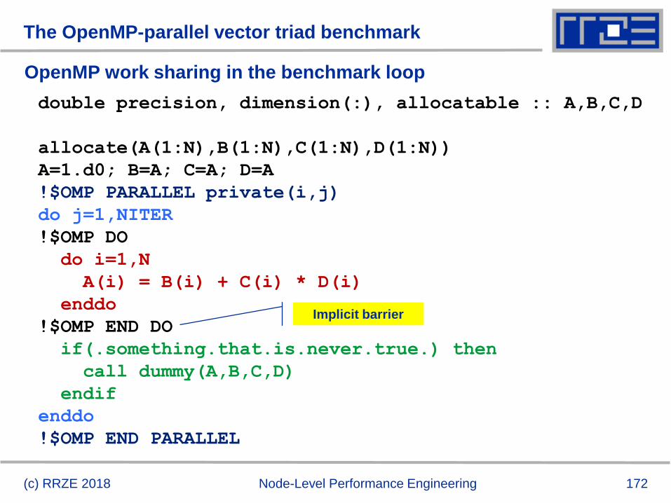
172
The OpenMP-parallel vector triad benchmark
OpenMP work sharing in the benchmark loop
(c) RRZE 2018 Node-Level Performance Engineering
double precision, dimension(:), allocatable :: A,B,C,D
allocate(A(1:N),B(1:N),C(1:N),D(1:N))
A=1.d0; B=A; C=A; D=A
!$OMP PARALLEL private(i,j)
do j=1,NITER
!$OMP DO
do i=1,N
A(i) = B(i) + C(i) * D(i)
enddo
!$OMP END DO
if(.something.that.is.never.true.) then
call dummy(A,B,C,D)
endif
enddo
!$OMP END PARALLEL
Implicit barrier
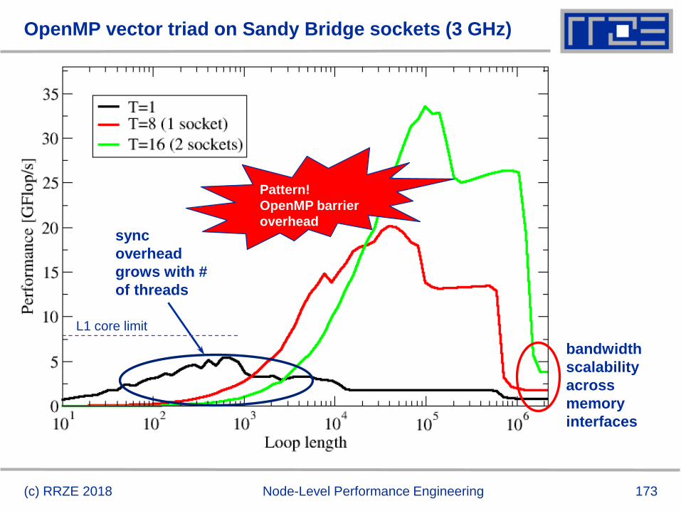
173
OpenMP vector triad on Sandy Bridge sockets (3 GHz)
(c) RRZE 2018 Node-Level Performance Engineering
sync
overhead
grows with #
of threads
bandwidth
scalability
across
memory
interfaces
L1 core limit
Pattern!
OpenMP barrier
overhead
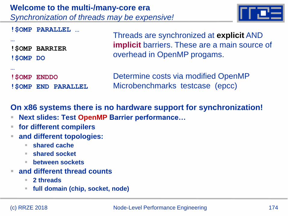
174(c) RRZE 2018 Node-Level Performance Engineering
Welcome to the multi-/many-core era
Synchronization of threads may be expensive!
!$OMP PARALLEL …
…
!$OMP BARRIER
!$OMP DO
…
!$OMP ENDDO
!$OMP END PARALLEL
On x86 systems there is no hardware support for synchronization!
Next slides: Test OpenMP Barrier performance…
for different compilers
and different topologies:
shared cache
shared socket
between sockets
and different thread counts
2 threads
full domain (chip, socket, node)
Threads are synchronized at explicit AND
implicit barriers. These are a main source of
overhead in OpenMP progams.
Determine costs via modified OpenMP
Microbenchmarks testcase (epcc)
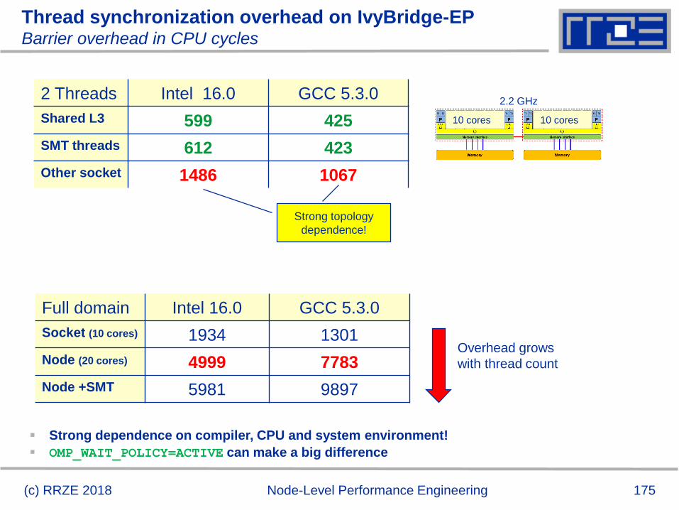
175(c) RRZE 2018 Node-Level Performance Engineering
Thread synchronization overhead on IvyBridge-EP Barrier overhead in CPU cycles
2 Threads Intel 16.0 GCC 5.3.0
Shared L3 599 425
SMT threads 612 423
Other socket 1486 1067
Full domain Intel 16.0 GCC 5.3.0
Socket (10 cores) 1934 1301
Node (20 cores) 4999 7783
Node +SMT 5981 9897
Strong topology
dependence!
10 cores 10 cores
2.2 GHz
Strong dependence on compiler, CPU and system environment!
OMP_WAIT_POLICY=ACTIVE can make a big difference
Overhead grows
with thread count
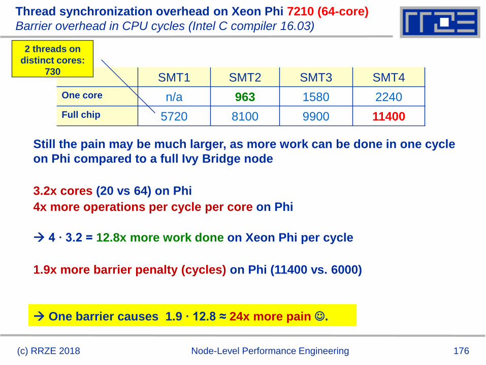
176(c) RRZE 2018 Node-Level Performance Engineering
Thread synchronization overhead on Xeon Phi 7210 (64-core)
Barrier overhead in CPU cycles (Intel C compiler 16.03)
SMT1 SMT2 SMT3 SMT4
One core n/a 963 1580 2240
Full chip 5720 8100 9900 11400
Still the pain may be much larger, as more work can be done in one cycle
on Phi compared to a full Ivy Bridge node
3.2x cores (20 vs 64) on Phi
4x more operations per cycle per core on Phi
4 ∙ 3.2 = 12.8x more work done on Xeon Phi per cycle
1.9x more barrier penalty (cycles) on Phi (11400 vs. 6000)
One barrier causes 1.9 ∙ 12.8 ≈ 24x more pain .
2 threads on
distinct cores:
730
Pattern-driven
Performance Engineering
Basics of Benchmarking
Performance Patterns
Signatures
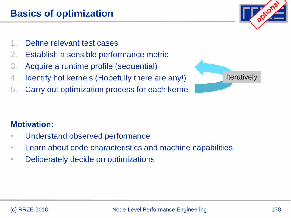
178
Basics of optimization
1. Define relevant test cases
2. Establish a sensible performance metric
3. Acquire a runtime profile (sequential)
4. Identify hot kernels (Hopefully there are any!)
5. Carry out optimization process for each kernel
Motivation:
• Understand observed performance
• Learn about code characteristics and machine capabilities
• Deliberately decide on optimizations
Iteratively
(c) RRZE 2018 Node-Level Performance Engineering
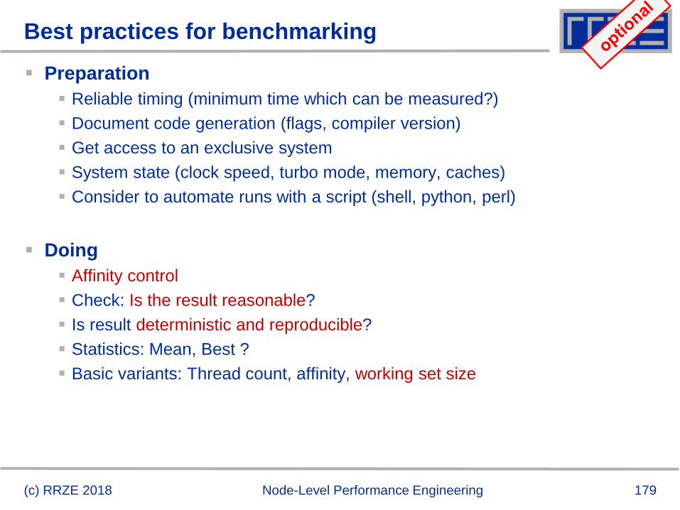
179
Best practices for benchmarking
Preparation
Reliable timing (minimum time which can be measured?)
Document code generation (flags, compiler version)
Get access to an exclusive system
System state (clock speed, turbo mode, memory, caches)
Consider to automate runs with a script (shell, python, perl)
Doing
Affinity control
Check: Is the result reasonable?
Is result deterministic and reproducible?
Statistics: Mean, Best ?
Basic variants: Thread count, affinity, working set size
Node-Level Performance Engineering(c) RRZE 2018
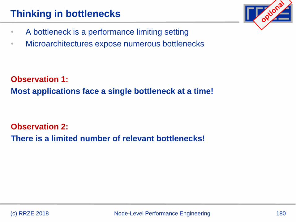
180
Thinking in bottlenecks
• A bottleneck is a performance limiting setting
• Microarchitectures expose numerous bottlenecks
Observation 1:
Most applications face a single bottleneck at a time!
Observation 2:
There is a limited number of relevant bottlenecks!
(c) RRZE 2018 Node-Level Performance Engineering
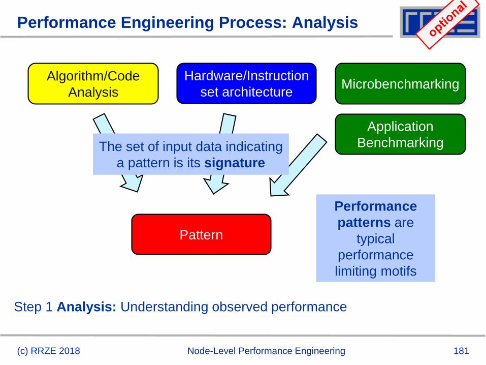
181
Performance Engineering Process: Analysis
Node-Level Performance Engineering
Pattern
MicrobenchmarkingHardware/Instruction
set architecture
Algorithm/Code
Analysis
Application
Benchmarking
Step 1 Analysis: Understanding observed performance
Performance
patterns are
typical
performance
limiting motifs
The set of input data indicating
a pattern is its signature
(c) RRZE 2018
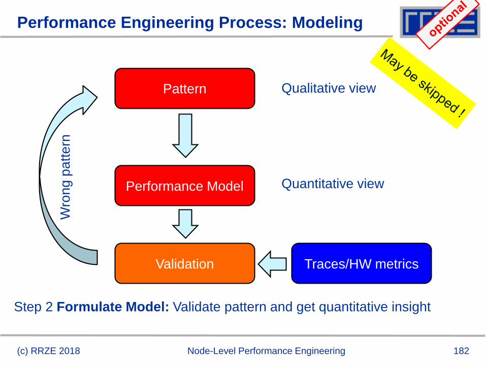
182
Performance Engineering Process: Modeling
Node-Level Performance Engineering
Pattern
Performance Model
Qualitative view
Quantitative view
Step 2 Formulate Model: Validate pattern and get quantitative insight
Validation Traces/HW metrics
Wro
ng
pa
tte
rn
(c) RRZE 2018
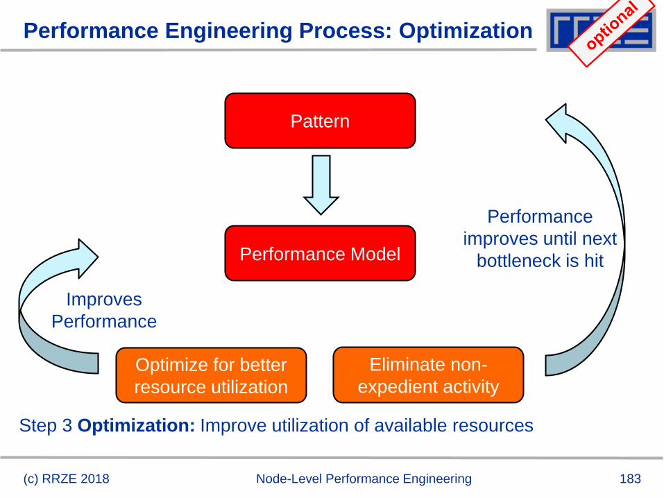
183
Performance Engineering Process: Optimization
Node-Level Performance Engineering
Optimize for better
resource utilization
Eliminate non-
expedient activity
Pattern
Performance Model
Performance
improves until next
bottleneck is hit
Improves
Performance
Step 3 Optimization: Improve utilization of available resources
(c) RRZE 2018
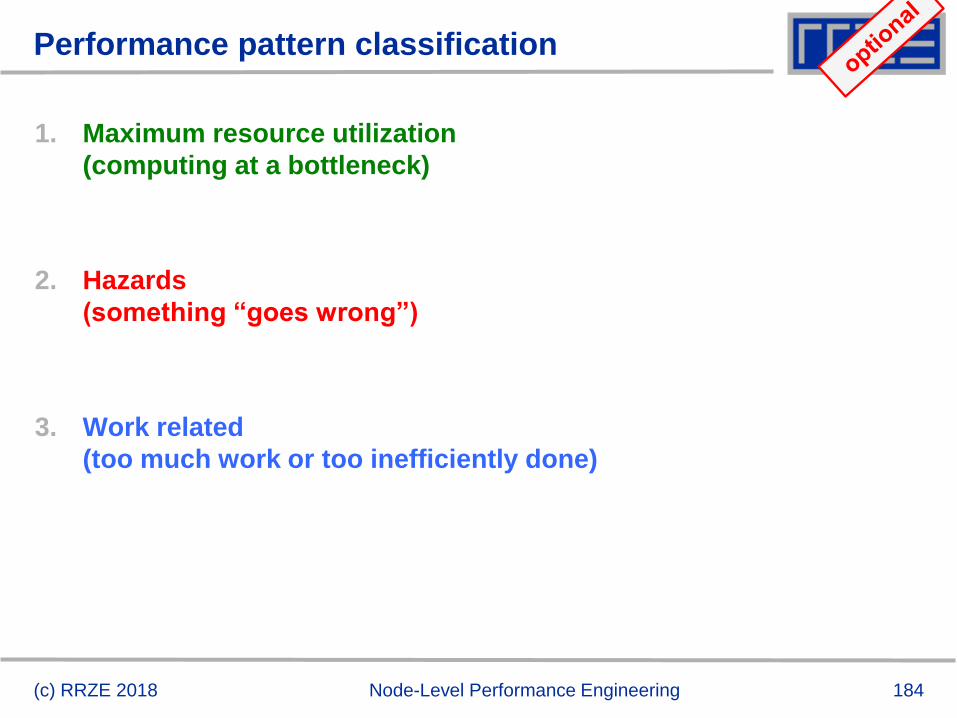
184
Performance pattern classification
1. Maximum resource utilization
(computing at a bottleneck)
2. Hazards
(something “goes wrong”)
3. Work related
(too much work or too inefficiently done)
(c) RRZE 2018 Node-Level Performance Engineering
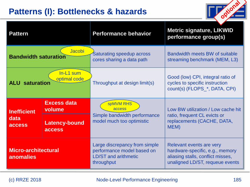
185
Patterns (I): Bottlenecks & hazards
Pattern Performance behaviorMetric signature, LIKWID
performance group(s)
Bandwidth saturationSaturating speedup across
cores sharing a data path
Bandwidth meets BW of suitable
streaming benchmark (MEM, L3)
ALU saturation Throughput at design limit(s)
Good (low) CPI, integral ratio of
cycles to specific instruction
count(s) (FLOPS_*, DATA, CPI)
Inefficient
data
access
Excess data
volumeSimple bandwidth performance
model much too optimistic
Low BW utilization / Low cache hit
ratio, frequent CL evicts or
replacements (CACHE, DATA,
MEM)Latency-bound
access
Micro-architectural
anomalies
Large discrepancy from simple
performance model based on
LD/ST and arithmetic
throughput
Relevant events are very
hardware-specific, e.g., memory
aliasing stalls, conflict misses,
unaligned LD/ST, requeue events
Jacobi
In-L1 sum
optimal code
spMVM RHS
access
(c) RRZE 2018 Node-Level Performance Engineering
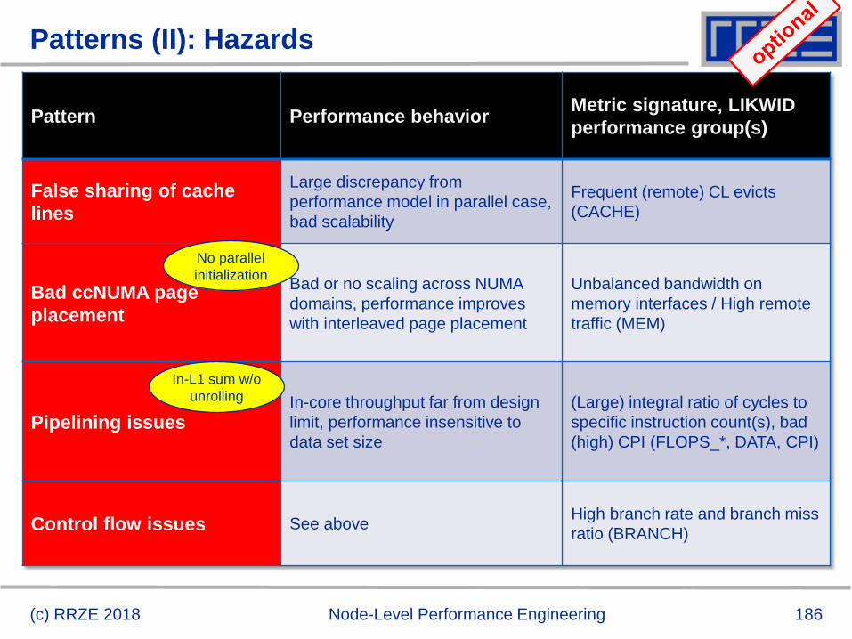
186
Patterns (II): Hazards
Pattern Performance behaviorMetric signature, LIKWID
performance group(s)
False sharing of cache
lines
Large discrepancy from
performance model in parallel case,
bad scalability
Frequent (remote) CL evicts
(CACHE)
Bad ccNUMA page
placement
Bad or no scaling across NUMA
domains, performance improves
with interleaved page placement
Unbalanced bandwidth on
memory interfaces / High remote
traffic (MEM)
Pipelining issuesIn-core throughput far from design
limit, performance insensitive to
data set size
(Large) integral ratio of cycles to
specific instruction count(s), bad
(high) CPI (FLOPS_*, DATA, CPI)
Control flow issues See aboveHigh branch rate and branch miss
ratio (BRANCH)
No parallel
initialization
In-L1 sum w/o
unrolling
(c) RRZE 2018 Node-Level Performance Engineering
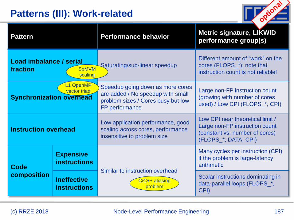
187
Patterns (III): Work-related
Pattern Performance behaviorMetric signature, LIKWID
performance group(s)
Load imbalance / serial
fractionSaturating/sub-linear speedup
Different amount of “work” on the
cores (FLOPS_*); note that
instruction count is not reliable!
Synchronization overhead
Speedup going down as more cores
are added / No speedup with small
problem sizes / Cores busy but low
FP performance
Large non-FP instruction count
(growing with number of cores
used) / Low CPI (FLOPS_*, CPI)
Instruction overheadLow application performance, good
scaling across cores, performance
insensitive to problem size
Low CPI near theoretical limit /
Large non-FP instruction count
(constant vs. number of cores)
(FLOPS_*, DATA, CPI)
Code
composition
Expensive
instructions
Similar to instruction overhead
Many cycles per instruction (CPI)
if the problem is large-latency
arithmetic
Ineffective
instructions
Scalar instructions dominating in
data-parallel loops (FLOPS_*,
CPI)
L1 OpenMP
vector triad
C/C++ aliasing
problem
(c) RRZE 2018 Node-Level Performance Engineering
SpMVM
scaling
188
Patterns conclusion
Pattern signature = performance behavior + hardware metrics
Patterns are applies hotspot (loop) by hotspot
Patterns map to typical execution bottlenecks
Patterns are extremely helpful in classifying performance issues
The first pattern is always a hypothesis
Validation by tanking data (more performance behavior, HW metrics)
Refinement or change of pattern
Performance models are crucial for most patterns
Model follows from pattern
(c) RRZE 2018 Node-Level Performance Engineering
189
Tutorial conclusion
Multicore architecture == multiple complexities
Affinity matters pinning/binding is essential
Bandwidth bottlenecks inefficiency is often made on the chip level
Topology dependence of performance features know your hardware!
Put cores to good use
Bandwidth bottlenecks surplus cores functional parallelism!?
Shared caches fast communication/synchronization better
implementations/algorithms?
Simple modeling techniques and patterns help us
… understand the limits of our code on the given hardware
… identify optimization opportunities
… learn more, especially when they do not work!
Simple tools get you 95% of the way
e.g., with the LIKWID tool suite
(c) RRZE 2018 Node-Level Performance Engineering
Most
powerful
tool?
190
THANK YOU.
(c) RRZE 2018 Node-Level Performance Engineering
Moritz Kreutzer
Markus Wittmann
Thomas Zeiser
Michael Meier
Holger Stengel
Thomas Gruber
Faisal Shahzad
Christie Louis Alappat
191(c) RRZE 2018 Node-Level Performance Engineering
Presenter Biographies
Georg Hager holds a PhD in computational physics from the University of Greifswald. He
is a senior research scientist in the HPC group at Erlangen Regional Computing Center
(RRZE). Recent research includes architecture-specific optimization for current
microprocessors, performance modeling on processor and system levels, and the efficient
use of hybrid parallel systems. His textbook “Introduction to High Performance Computing
for Scientists and Engineers” is required or recommended reading in many HPC-related
courses around the world. See his blog at http://blogs.fau.de/hager for current activities,
publications, and talks.
Jan Eitzinger (formerly Treibig) holds a PhD in Computer Science from the University of
Erlangen. He is now a postdoctoral researcher in the HPC Services group at Erlangen
Regional Computing Center (RRZE). His current research revolves around architecture-
specific and low-level optimization for current processor architectures, performance
modeling on processor and system levels, and programming tools. He is the developer of
LIKWID, a collection of lightweight performance tools. In his daily work he is involved in all
aspects of user support in High Performance Computing: training, code parallelization,
profiling and optimization, and the evaluation of novel computer architectures.
Gerhard Wellein holds a PhD in solid state physics from the University of Bayreuth and is
a professor at the Department for Computer Science at the University of Erlangen. He
leads the HPC group at Erlangen Regional Computing Center (RRZE) and has more than
ten years of experience in teaching HPC techniques to students and scientists from
computational science and engineering programs. His research interests include solving
large sparse eigenvalue problems, novel parallelization approaches, performance
modeling, and architecture-specific optimization.
192(c) RRZE 2018 Node-Level Performance Engineering
Abstract
SC18 full-day tutorial: Node-Level Performance Engineering
Presenter(s): Georg Hager, Gerhard Wellein
ABSTRACT:
The advent of multi- and manycore chips has led to a further opening of the gap between
peak and application performance for many scientific codes. This trend is accelerating as
we move from petascale to exascale. Paradoxically, bad node-level performance helps to
“efficiently” scale to massive parallelism, but at the price of increased overall time to
solution. If the user cares about time to solution on any scale, optimal performance on the
node level is often the key factor. We convey the architectural features of current
processor chips, multiprocessor nodes, and accelerators, as far as they are relevant for
the practitioner. Peculiarities like SIMD vectorization, shared vs. separate caches,
bandwidth bottlenecks, and ccNUMA characteristics are introduced, and the influence of
system topology and affinity on the performance of typical parallel programming
constructs is demonstrated. Performance engineering and performance patterns are
suggested as powerful tools that help the user understand the bottlenecks at hand and to
assess the impact of possible code optimizations. A cornerstone of these concepts is the
roofline model, which is described in detail, including useful case studies, limits of its
applicability, and possible refinements.
193
Selected references
Book:
G. Hager and G. Wellein: Introduction to High Performance Computing for Scientists and Engineers.
CRC Computational Science Series, 2010. ISBN 978-1439811924
https://blogs.fau.de/hager/hpc-book
Papers:
J. Hofmann, G. Hager, G. Wellein, and D. Fey: An analysis of core- and chip-level architectural
features in four generations of Intel server processors. In: J. Kunkel et al. (eds.), High Performance
Computing: 32nd International Conference, ISC High Performance 2017, Frankfurt, Germany, June 18-
22, 2017, Proceedings, Springer, Cham, LNCS 10266, ISBN 978-3-319-58667-0 (2017), 294-314.
DOI: 10.1007/978-3-319-58667-0_16. Preprint: arXiv:1702.07554
J. Hammer, J. Eitzinger, G. Hager, and G. Wellein: Kerncraft: A Tool for Analytic Performance
Modeling of Loop Kernels. In: Niethammer C., Gracia J., Hilbrich T., Knüpfer A., Resch M., Nagel W.
(eds), Tools for High Performance Computing 2016, ISBN 978-3-319-56702-0, 1-22 (2017).
Proceedings of IPTW 2016, the 10th International Parallel Tools Workshop, October 4-5, 2016,
Stuttgart, Germany. Springer, Cham. DOI: 10.1007/978-3-319-56702-0_1, Preprint: arXiv:1702.04653
J. Hofmann, D. Fey, M. Riedmann, J. Eitzinger, G. Hager, and G. Wellein: Performance analysis of the
Kahan-enhanced scalar product on current multi- and manycore processors. Concurrency &
Computation: Practice & Experience (2016). Available online, DOI: 10.1002/cpe.3921. Preprint:
arXiv:1604.01890
M. Röhrig-Zöllner, J. Thies, M. Kreutzer, A. Alvermann, A. Pieper, A. Basermann, G. Hager, G.
Wellein, and H. Fehske: Increasing the performance of the Jacobi-Davidson method by blocking. SIAM
Journal on Scientific Computing, 37(6), C697–C722 (2015). DOI: 10.1137/140976017,
Preprint:http://elib.dlr.de/89980/
(c) RRZE 2018 Node-Level Performance Engineering
194
References
T. M. Malas, G. Hager, H. Ltaief, H. Stengel, G. Wellein, and D. E. Keyes: Multicore-optimized
wavefront diamond blocking for optimizing stencil updates. SIAM Journal on Scientific
Computing 37(4), C439-C464 (2015). DOI: 10.1137/140991133, Preprint: arXiv:1410.3060
J. Hammer, G. Hager, J. Eitzinger, and G. Wellein: Automatic Loop Kernel Analysis and Performance
Modeling With Kerncraft. Proc. PMBS15, the 6th International Workshop on Performance Modeling,
Benchmarking and Simulation of High Performance Computer Systems, in conjunction with ACM/IEEE
Supercomputing 2015 (SC15), November 16, 2015, Austin, TX. DOI: 10.1145/2832087.2832092,
Preprint: arXiv:1509.03778
M. Kreutzer, G. Hager, G. Wellein, A. Pieper, A. Alvermann, and H. Fehske: Performance Engineering
of the Kernel Polynomial Method on Large-Scale CPU-GPU Systems. Proc. IPDPS15.
DOI: 10.1109/IPDPS.2015.76, Preprint: arXiv:1410.5242
M. Wittmann, G. Hager, T. Zeiser, J. Treibig, and G. Wellein: Chip-level and multi-node analysis of
energy-optimized lattice-Boltzmann CFD simulations. Concurrency and Computation: Practice and
Experience (2015). DOI: 10.1002/cpe.3489 Preprint: arXiv:1304.7664
H. Stengel, J. Treibig, G. Hager, and G. Wellein: Quantifying performance bottlenecks of stencil
computations using the Execution-Cache-Memory model. Proc. ICS15,
DOI: 10.1145/2751205.2751240, Preprint: arXiv:1410.5010
M. Kreutzer, G. Hager, G. Wellein, H. Fehske, and A. R. Bishop: A unified sparse matrix data format
for modern processors with wide SIMD units. SIAM Journal on Scientific Computing 36(5), C401–
C423 (2014). DOI: 10.1137/130930352, Preprint: arXiv:1307.6209
G. Hager, J. Treibig, J. Habich and G. Wellein: Exploring performance and power properties of modern
multicore chips via simple machine models. Computation and Concurrency: Practice and Experience
(2013). DOI: 10.1002/cpe.3180, Preprint: arXiv:1208.2908
(c) RRZE 2018 Node-Level Performance Engineering
195
References
J. Treibig, G. Hager and G. Wellein: Performance patterns and hardware metrics on modern multicore
processors: Best practices for performance engineering. Workshop on Productivity and Performance
(PROPER 2012) at Euro-Par 2012, August 28, 2012, Rhodes Island, Greece. DOI: 10.1007/978-3-
642-36949-0_50. Preprint: arXiv:1206.3738
M. Wittmann, T. Zeiser, G. Hager, and G. Wellein: Comparison of Different Propagation Steps for
Lattice Boltzmann Methods. Computers & Mathematics with Applications (Proc. ICMMES 2011).
Available online, DOI: 10.1016/j.camwa.2012.05.002. Preprint:arXiv:1111.0922
M. Kreutzer, G. Hager, G. Wellein, H. Fehske, A. Basermann and A. R. Bishop: Sparse Matrix-vector
Multiplication on GPGPU Clusters: A New Storage Format and a Scalable Implementation. Workshop
on Large-Scale Parallel Processing 2012 (LSPP12),
DOI: 10.1109/IPDPSW.2012.211
J. Treibig, G. Hager, H. Hofmann, J. Hornegger and G. Wellein: Pushing the limits for medical image
reconstruction on recent standard multicore processors. International Journal of High Performance
Computing Applications, (published online before print).
DOI: 10.1177/1094342012442424
G. Wellein, G. Hager, T. Zeiser, M. Wittmann and H. Fehske: Efficient temporal blocking for stencil
computations by multicore-aware wavefront parallelization. Proc. COMPSAC 2009. DOI:
10.1109/COMPSAC.2009.82
M. Wittmann, G. Hager, J. Treibig and G. Wellein: Leveraging shared caches for parallel temporal
blocking of stencil codes on multicore processors and clusters. Parallel Processing Letters 20 (4), 359-
376 (2010).
DOI: 10.1142/S0129626410000296. Preprint: arXiv:1006.3148
(c) RRZE 2018 Node-Level Performance Engineering
196
References
J. Treibig, G. Hager and G. Wellein: LIKWID: A lightweight performance-oriented tool suite for x86
multicore environments. Proc. PSTI2010, the First International Workshop on Parallel Software Tools
and Tool Infrastructures, San Diego CA, September 13, 2010. DOI: 10.1109/ICPPW.2010.38. Preprint:
arXiv:1004.4431
G. Schubert, H. Fehske, G. Hager, and G. Wellein: Hybrid-parallel sparse matrix-vector multiplication
with explicit communication overlap on current multicore-based systems. Parallel Processing Letters
21(3), 339-358 (2011).
DOI: 10.1142/S0129626411000254
J. Treibig, G. Wellein and G. Hager: Efficient multicore-aware parallelization strategies for iterative
stencil computations. Journal of Computational Science 2 (2), 130-137 (2011). DOI
10.1016/j.jocs.2011.01.010
K. Iglberger, G. Hager, J. Treibig, and U. Rüde: Expression Templates Revisited: A Performance
Analysis of Current ET Methodologies. SIAM Journal on Scientific Computing 34(2), C42-C69
(2012). DOI: 10.1137/110830125, Preprint: arXiv:1104.1729
K. Iglberger, G. Hager, J. Treibig, and U. Rüde: High Performance Smart Expression Template Math
Libraries. 2nd International Workshop on New Algorithms and Programming Models for the Manycore
Era (APMM 2012) at HPCS 2012, July 2-6, 2012, Madrid, Spain. DOI: 10.1109/HPCSim.2012.6266939
J. Habich, T. Zeiser, G. Hager and G. Wellein: Performance analysis and optimization strategies for a
D3Q19 Lattice Boltzmann Kernel on nVIDIA GPUs using CUDA. Advances in Engineering Software
and Computers & Structures 42 (5), 266–272 (2011). DOI: 10.1016/j.advengsoft.2010.10.007
J. Treibig, G. Hager and G. Wellein: Multicore architectures: Complexities of performance prediction
for Bandwidth-Limited Loop Kernels on Multi-Core Architectures.
DOI: 10.1007/978-3-642-13872-0_1, Preprint: arXiv:0910.4865.
(c) RRZE 2018 Node-Level Performance Engineering