NOAAŒNASA Coastal Zone Color Scanner Reanalysis Effort · NOAA–NASA Coastal Zone Color Scanner Reanalysis Effort ... November 1996–June 1997 , ... 5900 Princess Garden Parkway,

NOAA–NASA Coastal Zone Color Scanner Reanalysis Effort

Watson W. Gregg, Margarita E. Conkright, John E. O’Reilly, Frederick S. Patt,Menghua H. Wang, James A. Yoder, and Nancy W. Casey

Satellite observations of global ocean chlorophyll span more than two decades. However, incompatibil-ities between processing algorithms prevent us from quantifying natural variability. We applied acomprehensive reanalysis to the Coastal Zone Color Scanner �CZCS� archive, called the National Oceanicand Atmospheric Administration and National Aeronautics and Space Administration �NOAA–NASA�CZCS reanalysis �NCR� effort. NCR consisted of �1� algorithm improvement �AI�, where CZCS process-ing algorithms were improved with modernized atmospheric correction and bio-optical algorithms and �2�blending where in situ data were incorporated into the CZCS AI to minimize residual errors. Globalspatial and seasonal patterns of NCR chlorophyll indicated remarkable correspondence with modernsensors, suggesting compatibility. The NCR permits quantitative analyses of interannual and inter-decadal trends in global ocean chlorophyll. © 2002 Optical Society of America

OCIS codes: 010.4450, 010.1290, 280.0280.

1. Introduction

NASA and the international scientific communitieshave established a record of nearly continuous,high-quality global ocean color observations fromspace since 1996. The Ocean Color and Tempera-ture Scanner �OCTS; November 1996–June 1997�,the Sea-viewing Wide Field-of-view Sensor �Sea-WiFS; September 1997–present�, and the Moderate-Resolution Imaging Spectroradiometer �MODIS;September 2000–present� have provided an unprec-

W. W. Gregg �[email protected]� is with the NationalAeronautics and Space Administration, Goddard Space FlightCenter, Greenbelt, Maryland 20771. M. E. Conkright is with theOcean Climate Laboratory, National Oceanic and AtmosphericAdministration, National Oceanographic Data Center, SilverSpring, Maryland 20910. J. E. O’Reilly is with the National Oce-anic and Atmospheric Administration, National Marine FisheriesService, Narragansett Laboratory, 28 Tarzwell Drive, Narragan-sett, Rhode Island 02882. F. S. Patt is with Science ApplicationsInternational Corporation�General Sciences Corporation, Belts-ville, Maryland 20707. M. Wang is with the University of Mary-land, Baltimore County, National Aeronautics and SpaceAdministration, Goddard Space Flight Center, Greenbelt, Mary-land 20771. J. A. Yoder is with the Graduate School of Oceanog-raphy, University of Rhode Island, Narragansett, Rhode Island02882. N. W. Casey is with Science Systems and Applications,Incorporated, 5900 Princess Garden Parkway, Suite 300, Lanham,Maryland 20706.

Received 9 August 2001; revised manuscript received 11 Decem-ber 2001.

0003-6935�02�091615-14$15.00�0© 2002 Optical Society of America

edented view of chlorophyll dynamics on global scalesby use of modern, sophisticated data processingmethods. A predecessor sensor, the Coastal ZoneColor Scanner �CZCS; November 1978–June 1986�,utilized processing methodologies and algorithmsthat are outdated by modern standards. Thus theCZCS archive is severely limited for scientific analy-ses of interannual and interdecadal variability.This is an issue of fundamental importance to thestudy of global change.

In response, the National Oceanic and Atmo-spheric Administration �NOAA� and NASA estab-lished an effort to reanalyze the CZCS record byutilizing advances in algorithms that are shared bymodern remote sensing missions. In this paper wedescribe the methods and results of this effort, calledthe NOAA–NASA CZCS Reanalysis Effort �NCR�.Our methods involve the application of �1� recent al-gorithms to CZCS data to enhance quality and pro-vide consistency with the modern sensors OCTS,SeaWiFS, and MODIS and �2� blending techniques1

combining satellite data and the extensive in situarchives maintained by the National OceanographicData Center �NODC� Ocean Climate Laboratory�OCL� to minimize bias and residual error.

Our objective is to provide a high-quality blendedsatellite in situ data set that will enable a consistentview of global surface ocean chlorophyll and the pri-mary production patterns in two observational timesegments �1978–1986 and 1996–present� spanningtwo decades. By reconstructing the historical CZCSdata set, we can gain new insights into the processes

20 March 2002 � Vol. 41, No. 9 � APPLIED OPTICS 1615

and interactions involved in producing the interan-nual and interdecadal chlorophyll signals.

2. Background

A. Coastal Zone Color Scanner and the Modern OceanColor Sensors

The CZCS was a demonstration mission with twoobjectives: �1� to establish the technological and sci-entific feasibility of mapping ocean phytoplanktonpigment concentrations from satellites and �2� to de-termine the improvements that must be made forsuccessful follow-on ocean color missions. TheCZCS amply demonstrated the first objective. Italso clearly indicated deficiencies in its design andoperations that required correction to meet the sci-entific objectives of a successor mission. In approx-imate order of priority, these deficiencies, or requiredimprovements, were

�1� the need for routine, continuous global synopticobservations;

�2� better methods to characterize aerosols;�3� the need for a dedicated calibration and valida-

tion program over the lifetime of the mission;�4� methods to account for multiple scattering by

aerosols and the interaction between scattering bymolecules and aerosols;

�5� better signal-to-noise ratios �SNRs�;�6� the need to produce estimates of chlorophyll, not

pigment;�7� new information about chromophoric dissolved

organic matter;�8� the need to account for whitecap and foam re-

flectance; and�9� improved pixel navigation.

All the modern global missions meet the scientificrequirements for ocean color observations. They arededicated, routine observational platforms. Theycontain spectral bands in the near-infrared region ofthe spectrum to enable improved determination ofaerosol characteristics. Dedicated, high-quality insitu calibration and validation activities were estab-lished before launch. Complex algorithms were de-veloped to account for aerosol multiple scattering andinteractions with molecules. SNRs were improvedso that all the global missions have at least 500:1 forthe visible wavelengths2 instead of 200:1 for theCZCS.3 All the missions produce chlorophyll distri-butions as the primary geophysical product. A newspectral band was included at short wavelengths�near 410 nm� to help determine the distribution andabundance of chromophoric dissolved organic matter.Whitecap and foam reflectance algorithms were de-veloped and refined. Finally, precise navigationmethods were developed prelaunch, including im-proved orbit determination, sensor attitude informa-tion, and geolocation algorithms.

B. Coastal Zone Color Scanner Algorithm Deficiencies

Of course, some of the deficiencies of the CZCS dataset, such as sensor design and operation activities,cannot be improved after the fact. However, recentadvances in our understanding of atmospheric andoceanic optical principles that affect ocean color ob-servations can be applied to the archive. The globalCZCS data archive generally available from theNASA Goddard Earth Sciences �GES� DistributedActive Archive Center �DAAC� was produced in 1989with algorithms that were standard for the time.4All the subsequent algorithm improvements �AIs� areutilized in the atmospheric correction and bio-opticalalgorithms for the modern sensors OCTS, SeaWiFS,and MODIS and in future sensors such as the me-dium resolution imaging spectrometer, Global Im-ager, and the visible infrared imaging radiometersuite.

The CZCS archive contains eight major algorithmdeficiencies compared with modern sensors: �1� cal-ibration, �2� navigation, �3� constant aerosol type, �4�single-scattering approximation for aerosols and noRayleigh–aerosol interaction, �5� production of pig-ment rather than chlorophyll, �6� lack of whitecapand foam reflectance correction, �7� lack of correctionto Rayleigh scattering because of nonstandard atmo-spheric pressure, �8� lack of accounting for water-leaving radiance at 670 nm in high chlorophyll.

These deficiencies affect the representation ofglobal chlorophyll and are a major reason for differ-ences observed between the CZCS era and the mod-ern satellite observations of chlorophyll �shown inSection 4�.

C. Blending of Coastal Zone Color Scanner and in situData for Analysis of Seasonal Variability

Gregg and Conkright1 combined the extensive ar-chive of NOAA NODC OCL chlorophyll data��130,000 profiles� with the global CZCS archive atthe GES DAAC using the blended analysis of Reyn-olds5 to improve the quality and accuracy of globalchlorophyll seasonal climatologies. The blendedanalysis produced a dramatically different represen-tation of global, regional, and seasonal chlorophylldistributions than the archived CZCS.1 Generally,the CZCS appeared to underestimate chlorophyllconcentrations globally by 8–35%. On regional andseasonal scales, larger underestimates were common�20–40%, and occasionally the differences exceeded100%�.

Although the blending approach appeared to haveimproved many of the deficiencies of the CZCS sea-sonal climatologies, vast areas of the ocean lacked insitu observations, limiting the ability of the method tocorrect for the deficiencies in the CZCS processing.Further improvements by use of the blended methodrequire better CZCS data.

3. Methods

There are two main components to the NCR: �1�CZCS AI and �2� blending with in situ data. The

1616 APPLIED OPTICS � Vol. 41, No. 9 � 20 March 2002

first component �AI� addresses the eight major algo-rithm deficiencies in the global data set to produce adata set compatible with the modern processingmethods used for OCTS, SeaWiFS, and MODIS.The second component �blending� improves the resid-ual errors by use of the extensive coincident in situdatabase maintained by NODC OCL.

A. Coastal Zone Color Scanner Algorithm Improvement

1. CalibrationA retrospective analysis of the CZCS record led to arevised calibration.6 This revision is utilized by thereanalysis effort. Subsequent to publication of therevised calibration, a residual uncorrected temporaldegradation trend in band 4 �670 nm� was discov-ered.7 This correction is applied in the CZCS AI tothe time component of the calibration to begin at orbit6750 instead of orbit 20,000.8 Also, masking forelectronic overshoot is provided by use of methodsdescribed by Evans and Gordon.6

2. NavigationPoor orbit and attitude information from theNimbus-7 spacecraft often produced degraded navi-gation of CZCS imagery. Typically, improvementhas required intensive supervised methods to adjustimagery to match coastlines. Coastlines are not al-ways available in the imagery. As a consequence,the global CZCS data set provided by the GES DAACprovides only navigation derived from the onboardspacecraft attitude information and orbit ephemeriswithout additional correction.

We undertook an assessment of the CZCS naviga-tion errors to determine whether they were suffi-ciently stable to be corrected by bias adjustmentapplied to the existing navigation. We adapted themethod of island targets, originally developed forSeaWiFS,9 to the CZCS. In this method, the imagedata from multiple bands �usually two� are filtered toclassify each pixel as land, water, or clouds. Islandsin the data are located as small groups of contiguousland pixels surrounded by water and uncontami-nated by clouds. Island centroids are computedwith the available navigation and matched with ref-erence island locations from a catalog based on theWorld Vector Shoreline database.9 The island loca-tion errors are then used to estimate and characterizethe navigation errors.

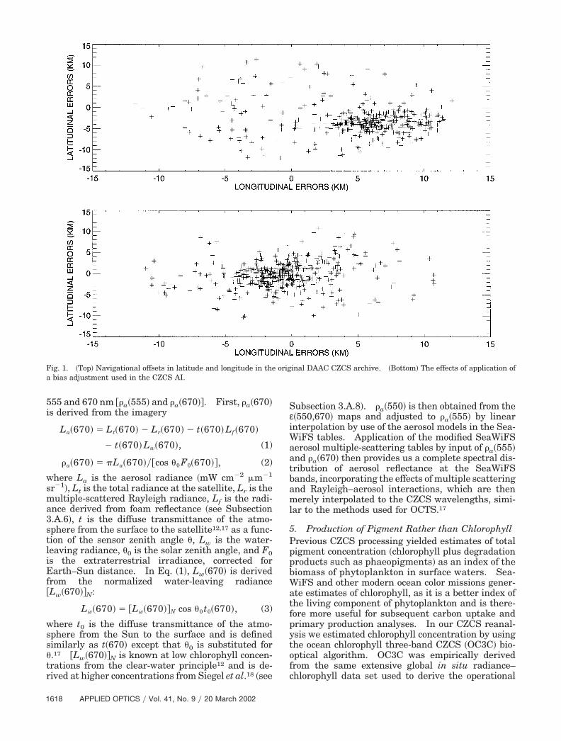
The method was adapted to use CZCS bands 1 �443nm� and 5 �750 nm� to avoid the saturation over landcommonly occurring in the middle CZCS wavelengths�520, 550, and 670 nm�. A Rayleigh-scattering cor-rection was applied to band 1, and both bands werenormalized to the solar zenith angle. We processeddata from two periods from the mission �February1980 and April 1982� to perform the initial analysis ofthe navigation errors. The results from both periodswere fairly consistent and showed errors that werenegative in latitude and positive in longitude. Theresults from April 1982 �Fig. 1� show a cluster ofpoints, centered on a latitudinal error of approxi-

mately �4 km and approximately 6 km in the longi-tudinal direction. The width of the cluster isapproximately �2 km in each direction. There are anumber of scattered points, mostly resulting fromisland mismatches or misclassified pixels.

We characterized these errors in terms of along-scan, along-track �orbit position�, and yaw �rotationabout nadir� offsets. We estimated the followingcorrections to navigation: 5.5 pixels along the scan,0.046 deg �5.9 km� along the track, and 0.18-deg yaw.We applied these corrections to the CZCS latitudesand longitudes and reprocessed the data from thesame periods. The results �Fig. 1� show that thetypical navigation errors are now close to zero, as canbe seen in the cluster points. The distribution ofpoints in the cluster is essentially the same and in-dicates some residual variation in the navigation er-rors. We processed other periods with thesecorrections and achieved similar results.

3. Constant Aerosol Type Representing Essentiallya Marine AerosolPrespecification of a constant aerosol type is one ofthe major deficiencies in the CZCS global dataset.10,11 However, it was a necessary deficiency be-cause variable aerosol types could be derived only byintensive supervised methods.12 We developed anunsupervised method to derive aerosol characteris-tics using standard meteorological techniques. Inour method, aerosol characteristics �defined by theaerosol reflectance ratio at 550 and 670 nm, orε�550,670�� are determined at every location in aCZCS image where clear-water conditions12 arevalid. Then the successive correction method13

�SCM� is used to extrapolate and interpolateε�550,670� values where the clear-water method isinvalid. Clear-water ε�550,670� values were ob-tained at local-area coverage resolution �approxi-mately 1 km� for each CZCS scene �an observationalsampling period, typically approximately 2 min oforbit time� for the mission life. We utilized local-area coverage processing to maximize the opportuni-ties for obtaining clear-water pixels. The ε�550,670�data were then assembled into daily representations,binned onto an 1800 � 900 equal-angle global grid,and the SCM was applied for each day. This pro-duced daily global maps of ε�550,670� values for theduration of the CZCS record with a resolution of ap-proximately 20 km.

4. Single-Scattering Approximations for Aerosolsand No Rayleigh–Aerosol InteractionAnother serious deficiency in the global CZCS dataset was the lack of a method to derive multiple-scattering aerosol reflectances and Rayleigh–aerosolinteraction.14,15 In the CZCS AI, we address thisdeficiency by utilizing the ε�550,670� global maps de-scribed above and modifying the SeaWiFS aerosolscattering tables16 to receive aerosol reflectance at


555 and 670 nm �a�555� and a�670��. First, a�670�is derived from the imagery

La�670� � Lt�670� � Lr�670� � t�670� Lf�670�

� t�670� Lw�670�, (1)

a�670� � La�670��cos �0 F0�670��, (2)

where La is the aerosol radiance �mW cm�2 �m�1

sr�1�, Lt is the total radiance at the satellite, Lr is themultiple-scattered Rayleigh radiance, Lf is the radi-ance derived from foam reflectance �see Subsection3.A.6�, t is the diffuse transmittance of the atmo-sphere from the surface to the satellite12,17 as a func-tion of the sensor zenith angle �, Lw is the water-leaving radiance, �0 is the solar zenith angle, and F0is the extraterrestrial irradiance, corrected forEarth–Sun distance. In Eq. �1�, Lw�670� is derivedfrom the normalized water-leaving radiance�Lw�670��N:

Lw�670� � �Lw�670��N cos �0 t0�670�, (3)

where t0 is the diffuse transmittance of the atmo-sphere from the Sun to the surface and is definedsimilarly as t�670� except that �0 is substituted for�.17 �Lw�670��N is known at low chlorophyll concen-trations from the clear-water principle12 and is de-rived at higher concentrations from Siegel et al.18 �see

Subsection 3.A.8�. a�550� is then obtained from theε�550,670� maps and adjusted to a�555� by linearinterpolation by use of the aerosol models in the Sea-WiFS tables. Application of the modified SeaWiFSaerosol multiple-scattering tables by input of a�555�and a�670� then provides us a complete spectral dis-tribution of aerosol reflectance at the SeaWiFSbands, incorporating the effects of multiple scatteringand Rayleigh–aerosol interactions, which are thenmerely interpolated to the CZCS wavelengths, simi-lar to the methods used for OCTS.17

5. Production of Pigment Rather than ChlorophyllPrevious CZCS processing yielded estimates of totalpigment concentration �chlorophyll plus degradationproducts such as phaeopigments� as an index of thebiomass of phytoplankton in surface waters. Sea-WiFS and other modern ocean color missions gener-ate estimates of chlorophyll, as it is a better index ofthe living component of phytoplankton and is there-fore more useful for subsequent carbon uptake andprimary production analyses. In our CZCS reanal-ysis we estimated chlorophyll concentration by usingthe ocean chlorophyll three-band CZCS �OC3C� bio-optical algorithm. OC3C was empirically derivedfrom the same extensive global in situ radiance–chlorophyll data set used to derive the operational

Fig. 1. �Top� Navigational offsets in latitude and longitude in the original DAAC CZCS archive. �Bottom� The effects of application ofa bias adjustment used in the CZCS AI.


SeaWiFS ocean chlorophyll four-band �OC4� algo-rithm.19 The equation for OC3C is

log C � 0.362 � 4.066R � 5.125R2 � 2.645R3

� 0.597R4, (4)

where C is the derived chlorophyll concentration �mgm�3� and R is the maximum reflectance ratio be-tween R1 and R2:

R1 ��Lw�N�443��F0�443�

�Lw�N�550��F0�550�, (5)

R2 ��Lw�N�520��F0�520�

�Lw�N�550��F0�550�. (6)

The equation for the SeaWiFS operational algo-rithm OC419 is

log C � 0.366 � 3.067R � 1.930R2 � 0.649R3

� 1.532 R4, (7)

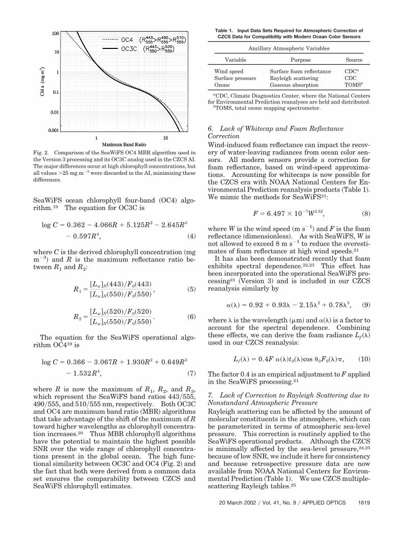
where R is now the maximum of R1, R2, and R3,which represent the SeaWiFS band ratios 443�555,490�555, and 510�555 nm, respectively. Both OC3Cand OC4 are maximum band ratio �MBR� algorithmsthat take advantage of the shift of the maximum of Rtoward higher wavelengths as chlorophyll concentra-tion increases.20 Thus MBR chlorophyll algorithmshave the potential to maintain the highest possibleSNR over the wide range of chlorophyll concentra-tions present in the global ocean. The high func-tional similarity between OC3C and OC4 �Fig. 2� andthe fact that both were derived from a common dataset ensures the comparability between CZCS andSeaWiFS chlorophyll estimates.

6. Lack of Whitecap and Foam ReflectanceCorrectionWind-induced foam reflectance can impact the recov-ery of water-leaving radiances from ocean color sen-sors. All modern sensors provide a correction forfoam reflectance, based on wind-speed approxima-tions. Accounting for whitecaps is now possible forthe CZCS era with NOAA National Centers for En-vironmental Prediction reanalysis products �Table 1�.We mimic the methods for SeaWiFS21:

F � 6.497 � 10�7W3.52, (8)

where W is the wind speed �m s�1� and F is the foamreflectance �dimensionless�. As with SeaWiFS, W isnot allowed to exceed 8 m s�1 to reduce the overesti-mates of foam reflectance at high wind speeds.21

It has also been demonstrated recently that foamexhibits spectral dependence.22,23 This effect hasbeen incorporated into the operational SeaWiFS pro-cessing21 �Version 3� and is included in our CZCSreanalysis similarly by

�� 0.92 � 0.93� � 2.15�2 � 0.78�3, (9)

where � is the wavelength ��m� and �� is a factor toaccount for the spectral dependence. Combiningthese effects, we can derive the foam radiance Lf ��used in our CZCS reanalysis:

Lf�� 0.4F ��t0��cos �0 F0��, (10)

The factor 0.4 is an empirical adjustment to F appliedin the SeaWiFS processing.21

7. Lack of Correction to Rayleigh Scattering due toNonstandard Atmospheric PressureRayleigh scattering can be affected by the amount ofmolecular constituents in the atmosphere, which canbe parameterized in terms of atmospheric sea-levelpressure. This correction is routinely applied to theSeaWiFS operational products. Although the CZCSis minimally affected by the sea-level pressure,24,25

because of low SNR, we include it here for consistencyand because retrospective pressure data are nowavailable from NOAA National Centers for Environ-mental Prediction �Table 1�. We use CZCS multiple-scattering Rayleigh tables.25

Fig. 2. Comparison of the SeaWiFS OC4 MBR algorithm used inthe Version 3 processing and its OC3C analog used in the CZCS AI.The major differences occur at high chlorophyll concentrations, butall values �25 mg m�3 were discarded in the AI, minimizing thesedifferences.

Table 1. Input Data Sets Required for Atmospheric Correction ofCZCS Data for Compatibility with Modern Ocean Color Sensors

Ancillary Atmospheric Variables

Variable Purpose Source

Wind speed Surface foam reflectance CDCa

Surface pressure Rayleigh scattering CDCOzone Gaseous absorption TOMSb

aCDC, Climate Diagnostics Center, where the National Centersfor Environmental Prediction reanalyses are held and distributed.

bTOMS, total ozone mapping spectrometer.


8. Lack of Accounting for Water-Leaving Radianceat 670 nm in High ChlorophyllAfter two years of SeaWiFS operations, it was discov-ered that where large chlorophyll concentrations ex-isted, substantial radiance in the near-infrared �NIR�bands �765 and 865 nm� left the water, violating theassumption of zero water-leaving radiance. Siegelet al.18 provided an iterative correction method toestimate the water-leaving radiance at these bandsand also at 670 nm for those who desired alternateatmospheric correction methods. The 670-nmmethod is directly applicable to the CZCS and is ap-plied in our reanalysis. Unlike SeaWiFS, however,the so-called NIR correction does not change the char-acterization of the aerosols in our CZCS reanalysis,just the amount. Aerosol characterization is derivedindependently from clear-water areas and is not af-fected by water-leaving radiance at 670 nm.

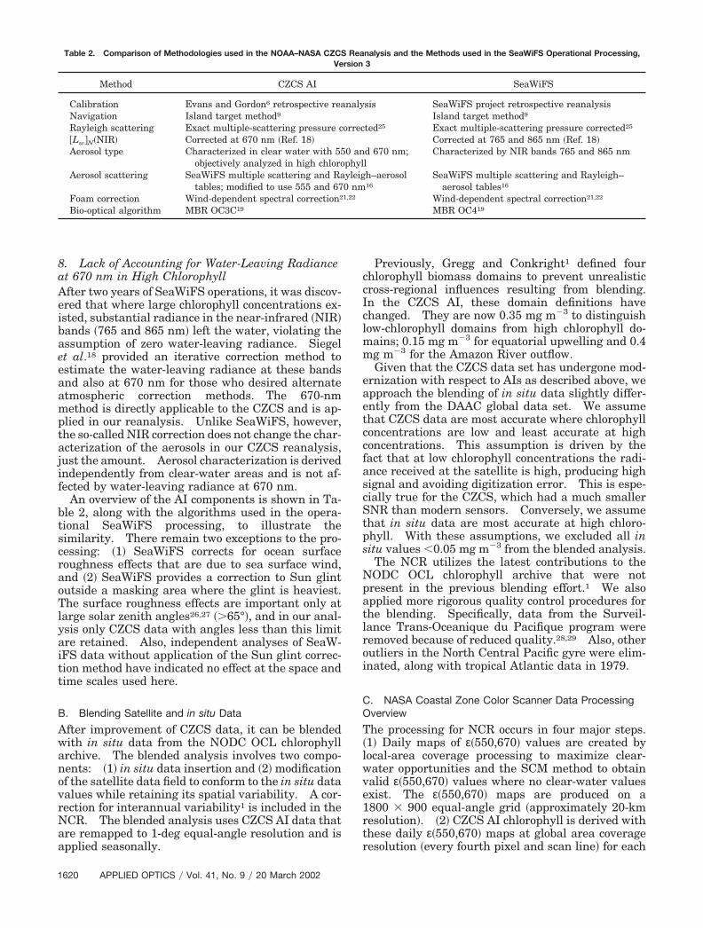
An overview of the AI components is shown in Ta-ble 2, along with the algorithms used in the opera-tional SeaWiFS processing, to illustrate thesimilarity. There remain two exceptions to the pro-cessing: �1� SeaWiFS corrects for ocean surfaceroughness effects that are due to sea surface wind,and �2� SeaWiFS provides a correction to Sun glintoutside a masking area where the glint is heaviest.The surface roughness effects are important only atlarge solar zenith angles26,27 ��65°�, and in our anal-ysis only CZCS data with angles less than this limitare retained. Also, independent analyses of SeaW-iFS data without application of the Sun glint correc-tion method have indicated no effect at the space andtime scales used here.

B. Blending Satellite and in situ Data

After improvement of CZCS data, it can be blendedwith in situ data from the NODC OCL chlorophyllarchive. The blended analysis involves two compo-nents: �1� in situ data insertion and �2� modificationof the satellite data field to conform to the in situ datavalues while retaining its spatial variability. A cor-rection for interannual variability1 is included in theNCR. The blended analysis uses CZCS AI data thatare remapped to 1-deg equal-angle resolution and isapplied seasonally.

Previously, Gregg and Conkright1 defined fourchlorophyll biomass domains to prevent unrealisticcross-regional influences resulting from blending.In the CZCS AI, these domain definitions havechanged. They are now 0.35 mg m�3 to distinguishlow-chlorophyll domains from high chlorophyll do-mains; 0.15 mg m�3 for equatorial upwelling and 0.4mg m�3 for the Amazon River outflow.

Given that the CZCS data set has undergone mod-ernization with respect to AIs as described above, weapproach the blending of in situ data slightly differ-ently from the DAAC global data set. We assumethat CZCS data are most accurate where chlorophyllconcentrations are low and least accurate at highconcentrations. This assumption is driven by thefact that at low chlorophyll concentrations the radi-ance received at the satellite is high, producing highsignal and avoiding digitization error. This is espe-cially true for the CZCS, which had a much smallerSNR than modern sensors. Conversely, we assumethat in situ data are most accurate at high chloro-phyll. With these assumptions, we excluded all insitu values �0.05 mg m�3 from the blended analysis.

The NCR utilizes the latest contributions to theNODC OCL chlorophyll archive that were notpresent in the previous blending effort.1 We alsoapplied more rigorous quality control procedures forthe blending. Specifically, data from the Surveil-lance Trans-Oceanique du Pacifique program wereremoved because of reduced quality.28,29 Also, otheroutliers in the North Central Pacific gyre were elim-inated, along with tropical Atlantic data in 1979.

C. NASA Coastal Zone Color Scanner Data ProcessingOverview

The processing for NCR occurs in four major steps.�1� Daily maps of ε�550,670� values are created bylocal-area coverage processing to maximize clear-water opportunities and the SCM method to obtainvalid ε�550,670� values where no clear-water valuesexist. The ε�550,670� maps are produced on a1800 � 900 equal-angle grid �approximately 20-kmresolution�. �2� CZCS AI chlorophyll is derived withthese daily ε�550,670� maps at global area coverageresolution �every fourth pixel and scan line� for each

Table 2. Comparison of Methodologies used in the NOAA–NASA CZCS Reanalysis and the Methods used in the SeaWiFS Operational Processing,Version 3

Method CZCS AI SeaWiFS

Calibration Evans and Gordon6 retrospective reanalysis SeaWiFS project retrospective reanalysisNavigation Island target method9 Island target method9

Rayleigh scattering Exact multiple-scattering pressure corrected25 Exact multiple-scattering pressure corrected25

�Lw�N�NIR� Corrected at 670 nm �Ref. 18� Corrected at 765 and 865 nm �Ref. 18�Aerosol type Characterized in clear water with 550 and 670 nm;

objectively analyzed in high chlorophyllCharacterized by NIR bands 765 and 865 nm

Aerosol scattering SeaWiFS multiple scattering and Rayleigh–aerosoltables; modified to use 555 and 670 nm16

SeaWiFS multiple scattering and Rayleigh–aerosol tables16

Foam correction Wind-dependent spectral correction21,22 Wind-dependent spectral correction21,22

Bio-optical algorithm MBR OC3C19 MBR OC419


scene of the mission lifetime �approximately 66,000scenes�. �3� CZCS AI global area coverage resolutionchlorophyll data are binned onto a 360 � 180 equal-angle grid �1-deg resolution� and into seasonal �3-month� temporal increments. This is performed foreach season and year for the CZCS record �1979–1986�. This coarse spatial and temporal resolutionenhances the effect of the blended analysis to correctresidual errors. �4� interannual variability correc-tions are derived, and then the blended analysis is

executed on seasonal climatologies. In addition,seasonal and yearly data are computed �no interan-nual variability correction is necessary� for each sea-son and year of the CZCS life.

We evaluate the results of the NCR by comparingthem with the 1989 CZCS data set available from theGES DAAC �called the DAAC CZCS�, where we con-verted pigment to chlorophyll using the algorithmsfrom O’Reilly et al.20 The NCR is also comparedwith a SeaWiFS seasonal climatology from launch

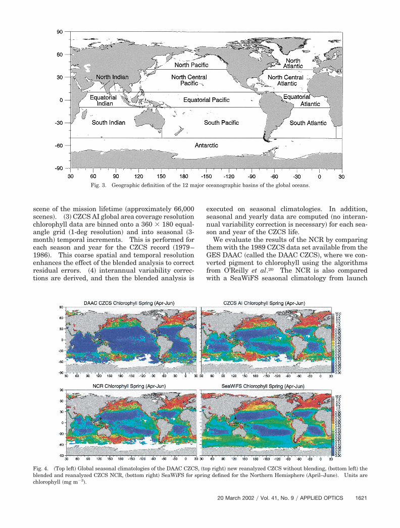
Fig. 3. Geographic definition of the 12 major oceanographic basins of the global oceans.

Fig. 4. �Top left� Global seasonal climatologies of the DAAC CZCS, �top right� new reanalyzed CZCS without blending, �bottom left� theblended and reanalyzed CZCS NCR, �bottom right� SeaWiFS for spring defined for the Northern Hemisphere �April–June�. Units arechlorophyll �mg m�3�.


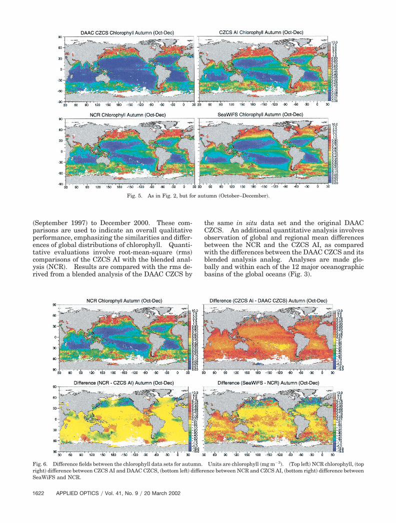
�September 1997� to December 2000. These com-parisons are used to indicate an overall qualitativeperformance, emphasizing the similarities and differ-ences of global distributions of chlorophyll. Quanti-tative evaluations involve root-mean-square �rms�comparisons of the CZCS AI with the blended anal-ysis �NCR�. Results are compared with the rms de-rived from a blended analysis of the DAAC CZCS by

the same in situ data set and the original DAACCZCS. An additional quantitative analysis involvesobservation of global and regional mean differencesbetween the NCR and the CZCS AI, as comparedwith the differences between the DAAC CZCS and itsblended analysis analog. Analyses are made glo-bally and within each of the 12 major oceanographicbasins of the global oceans �Fig. 3�.

Fig. 5. As in Fig. 2, but for autumn �October–December�.

Fig. 6. Difference fields between the chlorophyll data sets for autumn. Units are chlorophyll �mg m�3�. �Top left� NCR chlorophyll, �topright� difference between CZCS AI and DAAC CZCS, �bottom left� difference between NCR and CZCS AI, �bottom right� difference betweenSeaWiFS and NCR.


4. Results and Discussion

A. Comparison of the Coastal Zone Color ScannerAlgorithm Improvement and Reanalysis with SeaWiFS

Comparison of the CZCS AI and NCR chlorophyllwith SeaWiFS indicates a large degree of consis-tency �Figs. 4–6�. Seasons are defined accordingto the Northern Hemisphere convention: winter�January–March�, spring �April–June�, summer�July–September�, and autumn �October–December�.Sizes, shapes, and magnitudes of the mid-ocean gyresexhibit remarkable similarity. This is especially no-ticeable when compared with the DAAC CZCS pig-ment data converted to chlorophyll. The mid-oceangyres are particularly noteworthy—the DAAC CZCSgyres are vastly expanded relative to the CZCS re-analysis and SeaWiFS. These results suggest thatthe differences between the DAAC CZCS and Sea-WiFS are mostly due to algorithm differences and notto natural variability. The CZCS AI exhibits corre-spondence especially in the broad gyres. It is thislevel of correspondence that strongly indicates con-

sistency between these algorithms and the SeaWiFSalgorithms.

There are substantial differences between the NCRseasonal climatologies and SeaWiFS, such as thenorthern high latitudes in autumn and near NewZealand in spring. But the overall correspondencesuggests that these differences may be due to naturalvariability and not algorithms, which is the purposeof this effort.

We can obtain a quantitative understanding of theeffects of the NCR by determining the rms differencebetween the CZCS blended and the unblended fields�the AI in the case of the reanalyzed CZCS and theDAAC CZCS archive in the case of the historical ver-sion�. This analysis provides an index of the depar-ture of the blended fields from the original satellitefields and indicates how closely the two fields agree.A small rms difference indicates that the blendedanalysis made relatively minor adjustments to theoriginal satellite field and suggests agreement. Alarge rms indicates that the original satellite fielddeviates greatly from the in situ data and suggestspoor quality of the original satellite field.

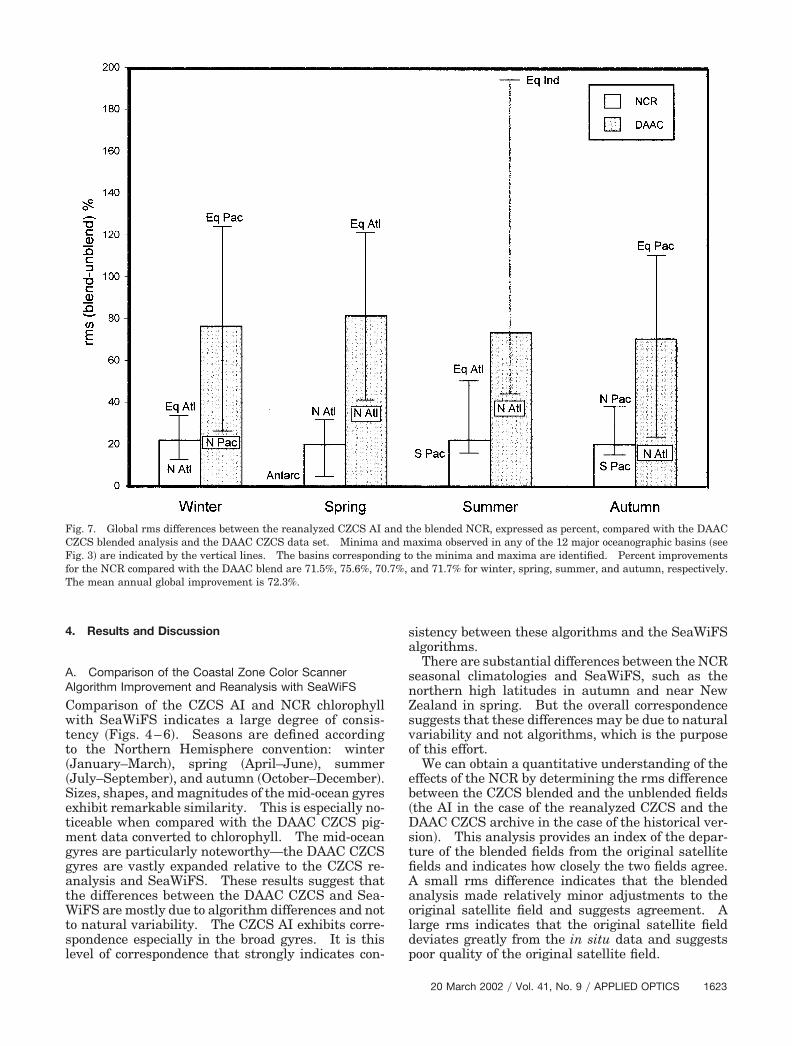
Fig. 7. Global rms differences between the reanalyzed CZCS AI and the blended NCR, expressed as percent, compared with the DAACCZCS blended analysis and the DAAC CZCS data set. Minima and maxima observed in any of the 12 major oceanographic basins �seeFig. 3� are indicated by the vertical lines. The basins corresponding to the minima and maxima are identified. Percent improvementsfor the NCR compared with the DAAC blend are 71.5%, 75.6%, 70.7%, and 71.7% for winter, spring, summer, and autumn, respectively.The mean annual global improvement is 72.3%.


The rms blended and unblended comparison indi-cates that the CZCS AI is a major improvement overthe DAAC CZCS �Fig. 7�. The previous DAAC CZCSblend represented a 70–81% change over the un-blended DAAC CZCS data. This compares with 20–22% for the change of the NCR to the CZCS AI. Thisstrongly suggests that blending of the CZCS AI doesnot introduce large deviations, and that it is thereforea higher quality and more accurate representation ofglobal ocean chlorophyll than the DAAC CZCS. Themoderate adjustments produced by the blending ofthe CZCS AI with in situ chlorophyll yield an overallimproved final product, which is the NCR.

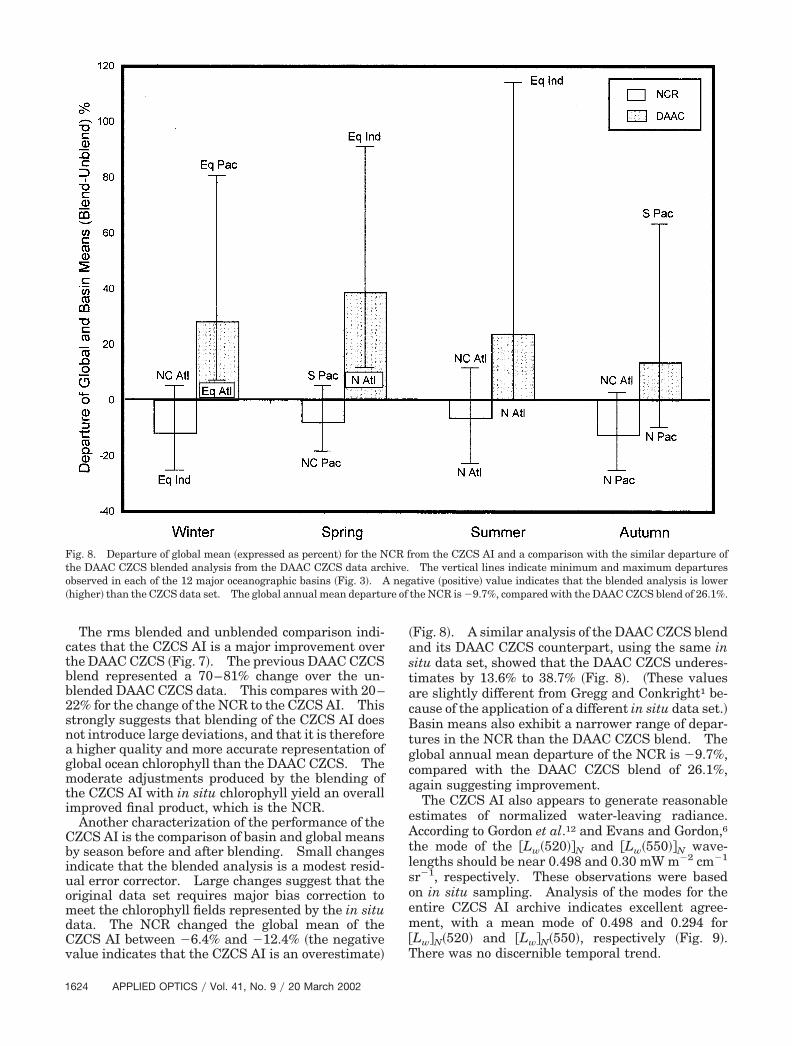
Another characterization of the performance of theCZCS AI is the comparison of basin and global meansby season before and after blending. Small changesindicate that the blended analysis is a modest resid-ual error corrector. Large changes suggest that theoriginal data set requires major bias correction tomeet the chlorophyll fields represented by the in situdata. The NCR changed the global mean of theCZCS AI between �6.4% and �12.4% �the negativevalue indicates that the CZCS AI is an overestimate�

�Fig. 8�. A similar analysis of the DAAC CZCS blendand its DAAC CZCS counterpart, using the same insitu data set, showed that the DAAC CZCS underes-timates by 13.6% to 38.7% �Fig. 8�. �These valuesare slightly different from Gregg and Conkright1 be-cause of the application of a different in situ data set.�Basin means also exhibit a narrower range of depar-tures in the NCR than the DAAC CZCS blend. Theglobal annual mean departure of the NCR is �9.7%,compared with the DAAC CZCS blend of 26.1%,again suggesting improvement.

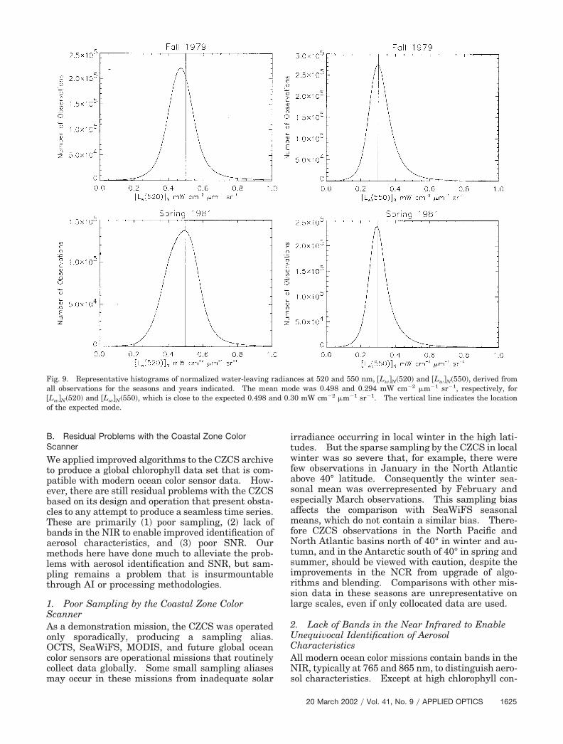
The CZCS AI also appears to generate reasonableestimates of normalized water-leaving radiance.According to Gordon et al.12 and Evans and Gordon,6the mode of the �Lw�520��N and �Lw�550��N wave-lengths should be near 0.498 and 0.30 mW m�2 cm�1

sr�1, respectively. These observations were basedon in situ sampling. Analysis of the modes for theentire CZCS AI archive indicates excellent agree-ment, with a mean mode of 0.498 and 0.294 for�Lw�N�520� and �Lw�N�550�, respectively �Fig. 9�.There was no discernible temporal trend.

Fig. 8. Departure of global mean �expressed as percent� for the NCR from the CZCS AI and a comparison with the similar departure ofthe DAAC CZCS blended analysis from the DAAC CZCS data archive. The vertical lines indicate minimum and maximum departuresobserved in each of the 12 major oceanographic basins �Fig. 3�. A negative �positive� value indicates that the blended analysis is lower�higher� than the CZCS data set. The global annual mean departure of the NCR is �9.7%, compared with the DAAC CZCS blend of 26.1%.


B. Residual Problems with the Coastal Zone ColorScanner

We applied improved algorithms to the CZCS archiveto produce a global chlorophyll data set that is com-patible with modern ocean color sensor data. How-ever, there are still residual problems with the CZCSbased on its design and operation that present obsta-cles to any attempt to produce a seamless time series.These are primarily �1� poor sampling, �2� lack ofbands in the NIR to enable improved identification ofaerosol characteristics, and �3� poor SNR. Ourmethods here have done much to alleviate the prob-lems with aerosol identification and SNR, but sam-pling remains a problem that is insurmountablethrough AI or processing methodologies.

1. Poor Sampling by the Coastal Zone ColorScannerAs a demonstration mission, the CZCS was operatedonly sporadically, producing a sampling alias.OCTS, SeaWiFS, MODIS, and future global oceancolor sensors are operational missions that routinelycollect data globally. Some small sampling aliasesmay occur in these missions from inadequate solar

irradiance occurring in local winter in the high lati-tudes. But the sparse sampling by the CZCS in localwinter was so severe that, for example, there werefew observations in January in the North Atlanticabove 40° latitude. Consequently the winter sea-sonal mean was overrepresented by February andespecially March observations. This sampling biasaffects the comparison with SeaWiFS seasonalmeans, which do not contain a similar bias. There-fore CZCS observations in the North Pacific andNorth Atlantic basins north of 40° in winter and au-tumn, and in the Antarctic south of 40° in spring andsummer, should be viewed with caution, despite theimprovements in the NCR from upgrade of algo-rithms and blending. Comparisons with other mis-sion data in these seasons are unrepresentative onlarge scales, even if only collocated data are used.

2. Lack of Bands in the Near Infrared to EnableUnequivocal Identification of AerosolCharacteristicsAll modern ocean color missions contain bands in theNIR, typically at 765 and 865 nm, to distinguish aero-sol characteristics. Except at high chlorophyll con-

Fig. 9. Representative histograms of normalized water-leaving radiances at 520 and 550 nm, �Lw�N�520� and �Lw�N�550�, derived fromall observations for the seasons and years indicated. The mean mode was 0.498 and 0.294 mW cm�2 �m�1 sr�1, respectively, for�Lw�N�520� and �Lw�N�550�, which is close to the expected 0.498 and 0.30 mW cm�2 �m�1 sr�1. The vertical line indicates the locationof the expected mode.


centrations,25 water is completely absorbing at thesewavelengths, and thus an unequivocal identificationof scattering aerosols is possible. �Absorbing aero-sols are difficult to identify with information only atthese NIR bands.� The CZCS had quantitativeocean-viewing bands at only 443, 520, 550, and 670nm, all of which are affected by chlorophyll. How-ever, at low chlorophyll concentrations, �Lw�520��N,�Lw�550��N, and �Lw�670��N are known.6,12 Ourmethod for deriving aerosol characteristics takes ad-vantage of the knowledge in these so-called clear-water areas and extrapolates to areas with highchlorophyll using standard methods developed formeteorology and applied to oceanographic prob-lems,30 called the SCM or also known as objectiveanalysis. The success of this methodology to repro-duce the spatial variability of aerosols depends on thenumber of observations over clear water. Occasion-ally individual CZCS scenes contained no valid oceanpixels other than high chlorophyll. For example,some scenes were mostly over land and containedonly a small fraction of high-chlorophyll coastal ar-eas. For this reason, we aggregate ε�550,670� over aday, so that there is the possibility of a preceding orsucceeding scene, or even a scene from a differentorbit, that can provide a clear-water ε�550,670� de-termination that is close enough to the high-chlorophyll pixels to be valid. Of course, it isimpossible for the SCM to detect aerosol fronts that

are located entirely within high chlorophyll. But ifthere are just a few clear water pixels within thehigh-chlorophyll regions and under the new aerosoltype, the SCM can resolve the front. Consideringthat the dynamics of ocean chlorophyll domains andaerosols are vastly different, it would seem an un-likely possibility that some detection of aerosol frontscannot be made, although it probably occurs occasion-ally.

To understand the sensitivity of the CZCS AI to theaerosol detection methodology, we prespecifiedε�520,670� and ε�550,670� to a fixed value of 1.0, rep-resenting a marine aerosol as in the DAAC CZCS.We applied our methodology otherwise identical tothe CZCS AI, including multiple-scattering aerosols.The global differences in spring and autumn wereonly 5.9% and 4.9%, respectively, compared with theAI with variable ε. The differences were only 2.5%and 3.3%, respectively, for spring and autumn, be-tween the blended results. These results illustratethe correction ability of the blended analysis. Thefixed ε experiment produced lower estimates of chlo-rophyll than the NCR, which is consistent with thealgorithm behavior and with the observations of un-derestimates in the DAAC CZCS.1

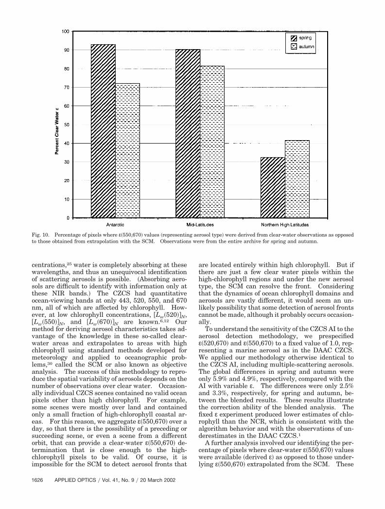
A further analysis involved our identifying the per-centage of pixels where clear-water ε�550,670� valueswere available �derived ε� as opposed to those under-lying ε�550,670� extrapolated from the SCM. These

Fig. 10. Percentage of pixels where ε�550,670� values �representing aerosol type� were derived from clear-water observations as opposedto those obtained from extrapolation with the SCM. Observations were from the entire archive for spring and autumn.


results indicate often high percentages of derived ε,especially in mid-latitudes �between �50° and 40°latitudes� �Fig. 10�. Reduced percentages of derivedε are observed in the northern high latitudes, buteven here, despite the massive spring bloom of highchlorophyll, there are still �30% of the chlorophyllpixels underlying derived ε values from low-chlorophyll �clear-water� regions. The Antarctic in-dicates generally good derived ε coverage.

3. Poor Signal-to-Noise RatiosThe CZCS SNRs, at approximately 200:1, are muchsmaller than modern sensors, with 500:1 or betternow common.3 This limits the dynamic range ofchlorophyll that the CZCS is able to detect, but moreimportantly may affect the quality of the derivedproducts. We minimize these effects by excludingall pixels where the water-leaving radiance diffuselytransmitted to the satellite �tLw��, where � � 443,520 and 550� is less than 2 digital counts. This en-sures sufficient signal in the data to exceed the noiselevel. In addition, the binning of ε�550,670� to a20-km grid involves averaging and thus reduces thesensitivity of the results to the low SNR.

5. Summary and Conclusions

We revised the CZCS global ocean chlorophyll ar-chive using compatible atmospheric correction andbio-optical algorithms with modern generation oceancolor sensors, such as OCTS, SeaWiFS, and MODIS.The revision involved two components: �1� AI,where CZCS processing algorithms were improved totake advantage of recent advances in atmosphericcorrection and bio-optical algorithms; and �2� blend-ing, where in situ data were incorporated into thefinal product to provide improvement of residual er-rors. The combination of the two components is re-ferred to as the NOAA–NASA CZCS reanalysis effort.The results of the NCR are compared with in situdata and indicate major improvement from the pre-viously available CZCS archive maintained by theNASA GES DAAC. Blending with in situ data pro-duced only a 21% adjustment to the CZCS AI field,compared with a 75% percent adjustment requiredfor the DAAC CZCS. This represented a 72% im-provement. Global annual means for the NCR sug-gested a small overestimate of 9.7% from the CZCSAI, compared with a mean 26% underestimate for theDAAC CZCS blend. Frequency distributions of nor-malized water-leaving radiances at 520 and 550 nmwere in close agreement with expected. Finally, ob-servations of global spatial and seasonal patterns in-dicated remarkable correspondence with SeaWiFS,suggesting data set compatibility.

This revision can permit a quantitative comparisonof the trends in global ocean chlorophyll from 1979–1986, when the CZCS sensor was active, to thepresent, beginning in 1996 with OCTS, SeaWiFS,and MODIS. The overall spatial and seasonal sim-ilarity of the data records of CZCS and SeaWiFSstrongly suggests that differences are due to naturalvariability, although some residual effects that are

due to CZCS sensor design or sampling may stillexist. We believe that this reanalysis of the CZCSarchives can enable identification of interannual andinterdecadal change. NCR CZCS data are availablethrough the GES DAAC.

We thank the NASA GES DAAC for the level-3SeaWiFS data, the level-1A CZCS data, and thelevel-3 CZCS archive data �in particular JamesAcker�, and the contributors of in situ data to theNOAA NODC archives. We also thank D. Antoinefor the revised decay function for CZCS band 4.H. R. Gordon and R. H. Evans are acknowledged foryears of analysis and characterization of the CZCSand whose research was fundamental to this revision.We also acknowledge the efforts of G. C. Feldman,W. E. Esaias, and C. R. McClain in the original globalprocessing of the CZCS archive. This research wassupported by NOAA’s Climate and Global ChangeProgram, NOAA–NASA Enhanced Data Sets Ele-ment, grant NOAA�RO#97-444�146-76-05 �W. W.Gregg and M. E. Conkright�, the NASA PathfinderData Set Research Program �M. E. Conkright, W. W.Gregg, J. E. O’Reilly, and J. A. Yoder�, and NASASensor Intercomparison and Merger for Biologicaland Interdisciplinary Oceanic Studies �SIMBIOS�grant NAS5-00203 �M. H. Wang�.

References1. W. W. Gregg and M. E. Conkright, “Global seasonal climatolo-

gies of ocean chlorophyll: blending in situ and satellite datafor the CZCS era,” J. Geophys. Res. 106, 2499–2515 �2001�.

2. International Ocean Color Coordinating Group, “Minimum re-quirements for an operational, ocean-color sensor for the openocean,” IOCCG Report 1. �IOCCG, Dartmouth, Nova Scotia,Canada, 1998�.

3. W. E. Esaias, M. R. Abbott, I. Barton, O. B. Brown, J. W.Campbell, K. L. Carder, D. K. Clark, R. H. Evans, F. E. Hoge,H. R. Gordon, W. M. Balch, R. Letelier, and P. J. Minnett, “Anoverview of MODIS capabilities for ocean science observa-tions,” IEEE Trans. Geosci. Remote Sens. 16, 1250–1265�1998�.

4. G. C. Feldman, N. Kuring, C. Ng, W. Esaias, C. R. McClain, J.Elrod, N. Maynard, D. Endres, R. Evans, J. Brown, S. Walsh,M. Carle, and G. Podesta, “Ocean color: availability of theglobal set,” Eos Trans. Am. Geophys. Union 70, 634–641�1989�.

5. R. W. Reynolds, “A real-time global sea surface temperatureanalysis,” J. Clim. 1, 75–86 �1988�.

6. R. H. Evans and H. R. Gordon, “Coastal Zone Color Scanner‘system calibration’: a retrospective examination,” J. Geo-phys. Res. 99, 7293–7307 �1994�.

7. R. H. Evans, Rosenstiel School of Marine and AtmosphericSciences, University of Miami, Miami, Fla. 33149 �personalcommunication, May 1999�.

8. D. Antoine, Laboratoire d’Oceanographie de Villefranche,06238 Villefranche sur Mer Cedex, France �personal commu-nication, January 2001�.

9. F. S. Patt, R. H. Woodward, and W. W. Gregg, “Automatednavigation assessment for Earth survey sensors using islandtargets,” Int. J. Remote Sens. 18, 3311–3336 �1997�.

10. H. R. Gordon and R. H. Evans, “Comment on ‘aerosol andRayleigh radiance contributions to Coastal Zone Colour Scan-ner images’ by Eckstein and Simpson,” Int. J. Remote Sens. 14,537–540 �1993�.

11. B. A. Eckstein and J. J. Simpson, “Aerosol and Rayleigh radi-


ance contributions to coastal zone colour scanner images,” Int.J. Remote Sens. 12, 135–168 �1991�.

12. H. R. Gordon, D. K. Clark, J. W. Brown, O. B. Brown, R. H.Evans, and W. W. Broenkow, “Phytoplankton pigment concen-trations in the Middle Atlantic Bight: comparison of shipdeterminations and CZCS estimates,” Appl. Opt. 22, 20–36�1983�.

13. R. Daley, Atmospheric Data Analysis �Cambridge U. Press,Cambridge, UK, 1991�.

14. D. L. Martin and M. J. Perry, “Minimizing systematic errorsfrom atmospheric multiple scattering and satellite viewinggeometry in coastal zone color scanner level IIA imagery,” J.Geophys. Res. 99, 7309–7322 �1994�.

15. H. R. Gordon and D. J. Castano, “Coastal Zone Color Scanneratmospheric correction algorithm: multiple scattering ef-fects,” Appl. Opt. 26, 2111–2122 �1987�.

16. H. R. Gordon and M. Wang, “Retrieval of water-leaving radi-ance and optical thickness over the oceans with SeaWiFS: apreliminary algorithm,” Appl. Opt. 33, 443–452 �1994�.

17. W. W. Gregg, F. S. Patt, and W. E. Esaias, “Initial analysis ofocean color data from OCTS. II. Geometric and radiometricanalysis,” Appl. Opt. 38, 5692–5702 �1999�.

18. D. A. Siegel, M. Wang, S. Maritorena, and W. Robinson, “At-mospheric correction of satellite ocean color imagery: theblack pixel assumption,” Appl. Opt. 39, 3582–3591 �2000�.

19. J. E. O’Reilly, S. Maritorena, D. A. Siegel, M. C. O’Brien, D.Toole, B. G. Mitchell, M. Kahru, F. P. Chavez, P. Strutton,G. F. Cota, S. B. Hooker, C. R. McClain, K. L. Carder, F.Muller-Karger, L. Harding, A. Magnuson, D. Phinney, G. F.Morre, J. Aiken, K. R. Arrigo, R. Letelier, and M. Culver,“Ocean color chlorophyll a algorithms for SeaWiFS, OC2 andOC4: Version 4,” in SeaWiFS Postlaunch Calibration andValidation Analyses, Part 3, NASA Tech. Memo. 2000-206892,Vol. 11, S. B. Hooker and E. R. Firestone, eds., �NASA GoddardSpace Flight Center, Greenbelt, Md., 2000�, pp. 8–22.

20. J. E. O’Reilly, S. Maritorena, B. G. Mitchell, D. A. Siegel, K. L.Carder, S. A. Garver, M. Kahru, and C. McClain, “Ocean colorchlorophyll algorithms for SeaWiFS,” J. Geophys. Res. 103,24937–24953 �1998�.

21. M. Wang, “The SeaWiFS atmospheric correction algorithm

updates,” in SeaWiFS Postlaunch Calibration and ValidationAnalyses, Part 1, NASA Tech. Memo. 2000-206892, Vol. 9, S. B.Hooker and E. R. Firestone, eds. �NASA Goddard Space FlightCenter, Greenbelt, Md., 2000�, pp. 57–63.

22. R. M. Frouin, M. Schwindling, and P. Y. Deschamps, “Spectralreflectance of sea foam in the visible and near infrared: insitu measurements and remote sensing implications,” J. Geo-phys. Res. 101, 14361–14371 �1996�.

23. K. R. Moore, K. J. Voss, and H. R. Gordon, “Spectral reflectanceof whitecaps: instrumentation, calibration, and performancein coastal waters,” J. Atmos. Oceanic Technol. 15, 496–509�1998�.

24. J.-M. Andre and A. Morel, “Simulated effects of barometricpressure and ozone content upon the estimate of marine phy-toplankton from space,” J. Geophys. Res. 94, 1029–1037�1989�.

25. H. R. Gordon, J. W. Brown, and R. H. Evans, “Exact Rayleighscattering calculations for use with the Nimbus-7 Coastal ZoneColor Scanner,” Appl. Opt. 27, 862–871 �1988�.

26. W. D. Robinson, G. M. Schmidt, C. R. McClain, and P. J.Werdell, “Changes made in the operational SeaWiFS process-ing,” in SeaWiFS Postlaunch Calibration and Validation Anal-yses, Part 3, NASA Tech. Memo. 2000-206892, Vol. 10., �NASAGoddard Space Flight Center, Greenbelt, Md., 2000�, pp. 12–28.

27. M. Wang, “The Rayleigh lookup tables for the SeaWiFS dataprocessing: accounting for the effects of ocean surface rough-ness,” Int. J. Remote Sens. �to be published�.

28. Y. Dandonneau, “A method for the rapid determination ofchlorophyll plus phaeopigments in samples collected by mer-chant ships,” Deep-Sea Res. 29, 647–654 �1982�.

29. Y. Dandonneau, “Surface chlorophyll concentration in thetropical Pacific Ocean: an analysis of data collected by mer-chant ships from 1978 to 1989,” J. Geophys. Res. 97, 3581–3591 �1992�.

30. M. E. Conkright, S. Levitus, T. O’Brien, T. P. Boyer, C. Ste-phens, D. Johnson, L. Stathoplos, O. Baranova, J. Antonov, R.Gelfeld, J. Burney, J. Rochester, and C. Forgy, “World oceandatabase 1998 CD-ROM data set documentation” �NationalOceanographic Data Center, Silver Spring, Md., 1998�.


Documents

NOAAŒNASA Coastal Zone Color Scanner Reanalysis Effort · NOAA–NASA Coastal Zone Color Scanner Reanalysis Effort ... November 1996–June 1997 , ... 5900 Princess Garden Parkway,