NOAA Technical Memorandum NOS NGS 24

DETERMINATION OF THE GEOPOTENTIAL FROM

SATELLITE-TO-SATELLITE TRACKING DATA

Rockville, Md January 1980

noaa NATIONAL OCEANIC AND ATMOSPHERIC ADMINISTRATION

/ National Ocean Survey

NOAA Technical Publications

National Ocean Survey/National Geodetic Survey subseries

The National Geodetic Survey (NGS) of the National Ocean Survey (NOS), NOAA, establishes and maintains the basic National horizontal and vertical networks of geodetic control and provides governmentwide leadership in the improvement of geodetic surveying methods and instrumentation, coordinates operations to assure network development, and provides specifications and criteria for survey operations by Federal, State, and other agencies.

NGS engages in research and development for the improvement of knowledge and its gravity field, and has the responsibility to procure geodetic data these data, and make them generally available to users through a central data

of the figure of the Earth from all sources, process base.

NOAA Technical Memorandums and some special NOAA publications are sold by the National Technical In­formation Service (NTIS) in paper copy and microfiche. Orders sho,uld be directed to NTIS, 5285 Port Royal Road, Springfield, VA 22161 (telephone: 703-557-4650). NTIS customer charge accounts are invited; some commercial charge accounts are accepted. When ordering, give the NTIS accession number (which begins with PB) shown in parentheses in the following citations.

Paper copies of NOAA Technical Reports, which are of general interest to the public, are sold by the Superintendent of Documents, U.S. Government Printing Office (GPO), Washington, DC 20402 (telephone: 202-783-3238). For prompt service, please furnish the GPO stock number with your order. If _a citation does not carry this number, then the publication is not sold by GPO. All NOAA Technical Reports may be purchased from NTIS in hard copy and microform. Prices for the same publication may vary between the two Government sales agents. Although both are nonprofit, GPO relies on some Federal support whereas NTIS is self-sustained.

An excellent reference source for Government publications is the National Depository Library program, a network of about 1,300 designated libraries. Requests for borrowing Depository Library material may be made through your local library. A free listing of libraries currently in this system is available from the Library Division, u.S. Government Printing Office, 5236 Eisenhower Ave., Alexandria, VA 22304 (telephone: 703-557-9013).

NOAA geodetic publications

Classification Standards of Accurac and General S ecifications of Geodetic Control Surve s. Federal Geodetic Control Committee, John O. Phillips Chairman), Department of Commerce, NOAA, NOS, 1974 reprinted annually, 12 pp (PB265442). National specifications and tables show the closures required and tolerances permitted for first-, second-, and third-order geodetic control surveys. (A single free copy can be obtained, upon request, from �he National Geodetic Survey, C13x4, NOS/NOAA, Rockville MD 20852.)

S ecifications To Su ort Classification Standards of Accurac and General S ecifications of Geodetic Control Surveys. Federal Geodetic Control Committee, John o. Phillips Chairman , Department of Com­merce, NOAA, NOS, 1975, reprinted annually, 30 pp (PB261037). This publication provides the rationale behind the original publication, "Classification, Standards of Accuracy, • • • 11 cited above. (A single free copy can be otained, upon request, from the National Geodetic Survey, C13x4, NOS/NOAA, Rockville MD 20852.)

Proceedings of the Second International Symposium on Problems Related to the Redefinition of North American Geodetic Networks. Sponsored by U.S. Department of Commerce; Department of Energy, Mines and Resources (Canada); and Danish Geodetic Institute; Arlington, Va., 1978, 658 pp. (GPO #003-017-0426-1). Fifty-four papers present the progress of the new adjustment of the North American Datum at mid­point, including reports by participating nations, software descriptions, nnd theoretical considera­tions.

NOS NGS-I

NOS NGS-2

NOAA Technical Memorandums, NOS/NGS subseries

Use of climatological and meteorological data in the planning and execution of National Geo­detic Survey field operations. Robert J. Leffler, December 1975, 30 pp (PB249677). Availa­bility, pertinence, uses. and procedures for using climatological and meteorological data are discussed as applicable to NGS field operations. Final report on responses to geodetic data questionnaire. John F. Spencer, Jr., March 1976, 39 pp (PB254641). Responses (20%) to a geodetic data questionnaire, mailed to 36,000 U.S. land surveyors, are analyzed for projecting future geodetic data needs.

(Continued at end of publication)

NOAA Technical Memorandum NOS NGS 24

DETERMINATION OF THE GEOPOTENTIAL FROM

SATELLITE-TO-SATELLITE TRACKING DATA

B. C. Douglas, C. C. Goad and F. F. Morrison

National Geodetic Survey Rockville, Md. January 1980

.-!l� UflTED STATES / NATIONAL OCEANIC AND / National Ocean A.'lr� DEPARTMENT Of COMMERCE ATMOSPHERIC ADMINISTRATION SUl'o'ey Il ....... M . ....... SlCfItIry Richard A. Frank. Administrator Herbert R. Lippold. Jr .• Director ( §

c:.�q,; .. �o)Y

Abstract

Introduction

CONTENTS

Representation of the Earth's gravity field

Simulation method

Simulation results

Discussion

Acknowledgment

References

1

1

2

6

14

. 24

27

28

DETERMINATION OF THE GEOPOTENTIAL FROM SATELLITE-TO-SATELLITE TRACKING DATA

Bruce C. Douglas Clyde C. Goad

F. Foster Morrison

National Geodetic Survey National Ocean Survey, NOAA

Rockville, Md. 20852

ABSTRACT. Simulations were made of the recovery of mean gravity anomalies from intersatellite Doppler measurements. A pair of surface-force compensated satellites was assumed to be in identical polar orbits, spaced by 3°, at an alti­tude of 200 km, taking intersatellite data with a preC1S1on of 0. 00 1 mm/ s . The results for a half-year mission indicate that 1°x 1° mean gravity anomalies can be obtained to a precision of a few milligals. A so-called high-low case, when one of the satellites is geosynchronous, appears to per­form about twice as well, but is probably imprac­tical to use because of the difficulty in obtain­ing the required data precision { 10-3 mm/s } with the long (-36,000 km) intersatellite distance involved. In contrast to previous analyses, our results are indicative of data obtainable from a global solution free of debatable a priori con­straints or assumptions about the geopotential. Thus a properly optimized mission using additional information, such as results from altimetry or mean surface anomalies, could improve upon the results presented here.

INTRODUCTION

The concept of using intersatellite measurements to determine the

geopotential is at least 10 years old (Wolff 1969). The advantage of this

scheme, compared to those based on ground-based observations, is continuous

global observation of orbital perturbations produced by the anomalous

geopotential.

2

The long wavelength variations of the geopotential, e. g. , n � 6, have been

determined satisfactorily from conventional satellite tracking data. Pro­

gress also has been made at very short wavelengths using GEOS-3 altimeter

data. Rapp (1979) reported lOxlo mean gravity anomalies from these data

precise to �7 mgal over most of the ocean surface. However, a global

determination of the gravity field to a higher precision would seem to

depend on a new satellite system.

For a believable simulation of the recovery of gravity field parameters,

the following conditions are necessary:

• The simulation should have a global character.

• The simulation should consider the effect of random and systematic

errors.

• The simulation should be independent of a priori information.

The last requirement may appear stringent, but adherence produces conserva­

tive conclusions.

REPRESENTATION OF THE EARTH'S GRAVITY FIELD

Spherical harmonics were unsuitable for our analyses because a complete

set of coefficients would have been required to model purely local effects.

A spherical harmonic model of degree and order 180 (l°x1° resolution ) would

require 32,400 coefficients. In addition, the computation of harmonics above

degree and order 70 requires special care (Chovitz et al. 1973). We chose

instead to represent lOxlo mean gravity anomalies by a surface layer of vari­

able density. In particular, we assumed the density X to be constant over a

small block, and represented the total field in terms of an aggregation of

such blocks.

Another representation, spherical harmonic sampling functions, has been

proposed by Giacaglia and Lundquist (1972). However, these have severe

computational problems. Sampling functions for a line, plane, or any

3

Cartesian Space R, can be generated by translation; i. e. , one needs only to

shift the argument by one division. For example, if we define

_ sin (2nx) So

(x) - 2nx

we can derive the remainder of the sampling functions from

Sk ex) = So

(x - k), k ±l, ±2, . . . .

Unfortunately, a simple symmetry condition does not exist for the spherical

domain, so one would have to invert 32,400 nonsparse matrices of dimension

32, 400 x 32,400 to obtain the functions, which would be represented by a

series with 32, 400 terms. Thus, technical and economic considerations

determined the use of a surface density model in these simulations. In ad­

dition, the ORAN (orbit analysis) computer program, described later, did not

have to be modified and retested extensively be fore using the density model

subroutines. The logic in Morrison's (1977) program was changed to accept

blocks o f arbitrary size (Morrison 1979). We did not use more sophisticated

means of analyzing the results, such as inversion theory (Kaula et al. 1978)

or collocation (Moritz 1978) because the project was designed to determine

the sensitivity and resolution unique to the proposed satellite-to-satellite

tracking systems.

The density o f a block is related to the usual mean gravity anomaly 6g

(Orlin 1959)

GX = � + l X N = �2n + 0.0368 N 2n 2 R

where G is the gravitational constant, y is global mean gravity, R is mean

Earth radius, N is geoid height (m), X is surface density, and 6g and GX are

in milligals • For most of the Earth, the approximation

6g ::: 2n G X

suffices for the purpose of error analysis.

4

Computing the acceleration o f a satellite resulting from a 10xlo density

layer block involves evaluation of a double integral. Some authors

approximate the solution of this integral by the attraction of one or more

point masses (Koch and Witte 1971). We used the solution of Morrison (1976,

1977). He evaluates one integral approximately analytically and the other

integral numerically. The advantage of this latter scheme is that the block

has no artificial "structure. " Unless a very large number of point masses

is used to approximate an individual density block, this structure creates

rapidly oscillating perturbations on a low altitude orbit, possibly leading

to erroneous conclusions.

The global rms (root mean square) mean gravity anomaly in 1° squares is

about 30 mgal. Because the uncertainty of 10xlo mean anomalies visible to

GEOS-3 over the ocean surface is less than 10 mgal, let us consider the

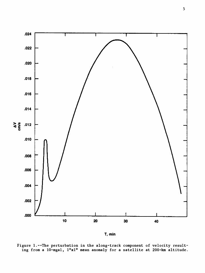
e ffect of a 10-mgal, 1 °xl 0 block on the speed of a near-Earth satellite.

Figure 1 shows the velocity perturbation in the along-track direction for a

satellite in a circular polar orbit passing directly over the block at an

altitude of 200 km.

Several interesting features appear in figure 1. First, note that the

block has two e ffects, a small high frequency perturbation of about

0. 006 cm/s, and a much larger low frequency (once/revolution) effect. This

latter e ffect comes from the overall perturbation vi the energy, and hence

period (Hotine and Morrison 1969). The effect does not contrib�te informa­

tion because every block will contain the effect and adjacent blocks cannot

be separable on this basis since the wavelength of the effect is vastly

greater than the dimensions of the blocks. The significant information about

a block appears in the sharp high frequency oscillation which occurs as the

satellite passes over a block. This oscillation persists, however, for a

considerable time (2-3 minutes) compared to the time required for a satel­

lite to traverse the 10xlo block (0. 25 minute). The fact that the perturba­

tion of a block persists over an along-track distance of about 10 times the

block size also means that adjacent 10xlo blocks will have a similar effect.

These will be hard to separate even when using the high frequency impulse.

It is also apparent that to maximize the relative along-track velocity per­

turbation between two satellites in identical low orbits the separation of

the satellites must be greater than 1°.

5

.024

.022

.020

.018

.016

.014

.010

.008

.006

.004

.002

.000 10 20 30 40

T,ml"

F igure l. --The perturbation in the along-track component of velocity result­ing from a lO-mgal, lOxlo mean anomaly for a satellite at 200-km altitude.

6

The magnitude of the velocity perturbation could be increased by choosing

a lower altitude, but 200 km is a reasonable height for a practical mission

after considering atmospheric drag forces. At this altitude the atmospheric

density scale height is only about 35 km, so the drag force is very sensi-

tive to small changes in altitude. In the discussion that follows, we

assume all satellites used surface-force compensation devices to eliminate

drag and radiation pressure effects.

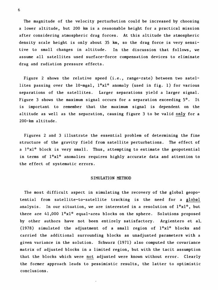
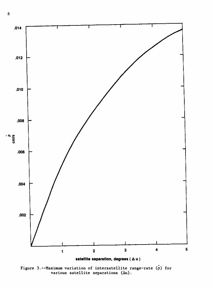
Figure 2 shows the relative speed (i. e. , range-rate) between two satel­

lites passing over the lO-mgal, 10xlo anomaly (used in fig. 1) for various

separations of the satellites. Larger separations yield a larger signal.

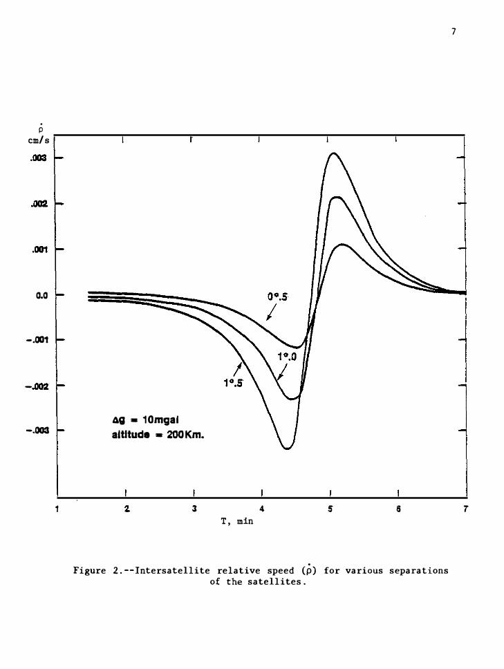
Figure 3 shows the maximum signal occurs for a separation exceeding 5°. It

is important to remember that the maximum signal is dependent on the

altitude as well as the separation, causing figure 3 to be valid only for a

200-km altitude.

Figures 2 and 3 illustrate the essential problem of determining the fine

structure of the gravity field from satellite perturbations. The effect of

a lOxlo block is very small. Thus, attempting to estimate the geopotential

in terms of 10xlo anomalies requires highly accurate data and attention to

the ef fect of systematic errors.

SIMULATION METHOD

The most di fficult aspect in simulating the recovery of the global geopo­

tential from satellite-to-satellite tracking is the need for a global

analysis. In our situation, we are interested in a resolution of 10xlo, but

there are 41,000 10xlo equal-area blocks on the sphere. Solutions proposed

by other authors have not been entirely satisfactory. Argientero et a1.

(1978) simulated the adjustment of a small region of 1 °xl ° blocks and

carried the additional surrounding blocks as unadjusted parameters with a

given variance in the solution. Schwarz (1971) also computed the covariance

matrix of adjusted blocks in a limited region, but with the tacit assumption

that the blocks which were not adjusted were known without error. Clearly

the former approach leads to pessimistic results, the latter to optimistic

conclusions.

·

p

cm/s

0.0

-.001

-.003

1

Ag - 10mgal

altitude - 200 Km.

3 T, min

4 s 6

Figure 2.--Intersatellite relative speed (p) for various separations of the satellites.

7

7

8

.014

.012

.010

.008

.006

.004

.002

1 2 3 4

satellite separation, degrees ( Au)

Figure 3.--Maximum variation of intersatellite range-rate (p) for various satellite separations (au).

5

9

Our approach for simulating a global solution was to simulate the recovery

of a region with dimensions large enough to allow the 10xlo anomalies near

the center of the region to be regarded as having essentially the same sta­

tistical properties in the solution that they would have possessed in a

global solution. Figure I shows the size of this region would have to be

substantial because the impulse-like perturbation of a 10xlo block persists

for a long time relative to the size of the block. We began our experiments

with a l5°xI5° region containing 225 I °xl ° mean gravity anomalies. To

verify that this region was large enough to ensure the central anomaly would

have the properties of a global solution, we simulated the recovery of a

larger 15°x25° region. Our results actually improved slightly for the

central region, giving us confidence that our conclusions would be

conservative.

Another problem in simulating the recovery of 10xlo gravity anomalies is

the tremendous amount of required orbital computations. In our example

using a region 15° widet many months of orbiting by polar satellites would

have been required to obtain dense overflights of the area. In addition, a

5-second numerical integration step size, with a multistep method is re­

quired because of the sharp, high frequency effect of lOx! ° anomalies. To

avoid this lengthy computation we considered independent orbital arcs only

over the region being considered. However, the initial conditions for each

arc were not adjusted. Our assumption was that the ephemerides of the two

satellites would be computed in long arc (a few days) solutions from ground

tracking.

The separation of the ephemeris computation from gravity anomaly

estimation requires justification, especially in relation to the effect of

systematic errors on the ephemerides. For example, the locations of ground

tracking stations are uncertain to some degree, and this error propagates

into the intersatellite range-rate measurement. Fortunately, this effect is

readily evaluated.

The usual least-squares solution relates observation residuals, 00, to

adjusted parameters, a, in the presence of data noise, e, by

10

<So = A oa + e (1)

where A is a matrix of partial derivatives of the measurements w ith respect

to the adjusted parameters. If unadjusted parameters with error, y, related

to the observations by a matrix of partials, K, are present, then the obser­

vation equation becomes

<So = A oa - K Y + e. (2)

If W -1 is the covariance matrix of the measurement noise, e, the minimum

variance solution oa, which ignores the error in the unadjusted parameters,

is biased by an amount

(3)

The effect of a unit value of the y parameters is given by

(4)

By using eq. (4), for example, we can predict in advance the effects of an

error in station location on any particular solution. This is important to

evaluate, especially in the present case, because of the smallness of the

perturbation of a lOxlo mean gravity anomaly.

Although eq. (4) is simple in principle, it is computationally complex.

For example, we can easily imagine a mission where 10 Doppler or laser

ground tracking stations would each observe two satellites for 6 months.

The partial derivative matrices A and K must be obtained by numerical inte­

gration of variational equations, and there are scores of these equations.

Many sources of potential systematic error can arise in orbit determina­

tion. The most prominent are geopotential and tracking station coordinate

errors. We did not consider geopotential error here because we have

assumed, of course, that the geopotential was being estim::tted. However,

tracking-station coordinate errors need to be considered.

11

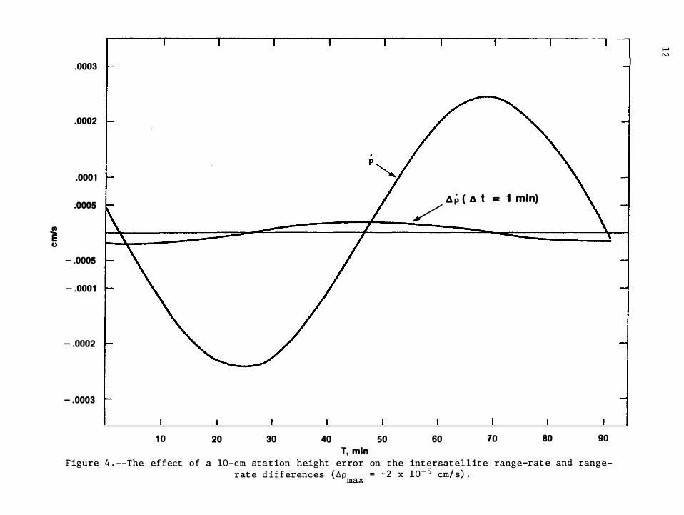
Using the computer program ORAN, which was developed around eq. (4), we

determined the effect of a 10-cm uncertainty in the height of one station

based on the initial conditions and the intersatellite range-rate measure­

ment, p, for two satellites spaced 30 apart in the same 200 -km altitude

polar orbit. The orbital arc length was 1 day with 15 Doppler tracking

sites well- distributed around the globe, using line-of-sight velocity

measurements of (J = 1 cm/s quality. The 10-cm value for the error of

station coordinates is realistic for the 1985 time frame. Figure 4 shows

the results.

Two significant aspects are apparent in figure 4. First, notice the long

period of the oscillation produced by the station coordinate error. This

effect, as noted before, occurs for orbital arcs more than a few revolutions

long and is caused by the dynamics of orbital motion. With modern instru­

ments, the timing error of observations is negligible, so that the orbital

period is extremely well -determined in long-arc solutions by repeated

passages over the tracking stations. Thus the satellite ephemeris can be in

error only periodically, as seen in figure 4. The effect of an error in the

location of an observing station is d ifferent from the effect of a localized

gravity anomaly, such as a 10xlo block, because the gravity anomaly causes a

distinct local change in the acceleration of the satellite.

The other important feature of figure 4 is the smallness of the effect of

the station coordinate error on the intersatellite range-rate. The ampli­

tude is 2.5 x 10-4 cm/s, about 5 percent of the impulse-like effect of a 10-

mgal, 1 °xl 0 anomaly block. Because the wavelength of the station-error

induced s ignal is more than 10 times the wavelength of the anomaly block

effect, one would anticipate little aliasing of one signal into the other.

But it is a simple matter to filter the intersatellite range-rate signal and

elim inate the error s ignal. To illustrate this, the low amplitude curve in

f igure 4 shows the effect of the station height error on the intersatellite

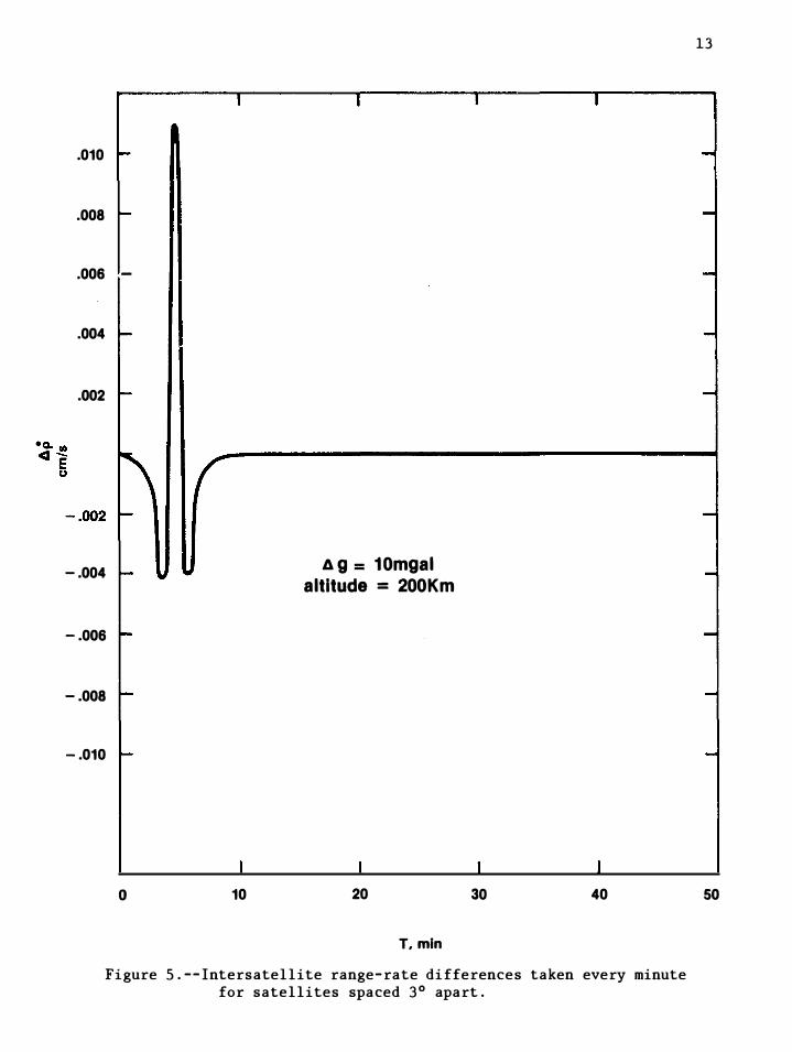
range-rate d ifference, llP taken over 1 minute. Figure 5 shows the corre­

sponding d ifferences of the range-rate oscillation produced by the 10-mgal,

1 °xl 0 block. As expected, the long wavelength signal is greatly reduced,

and the high frequency impulse-like s ignal is amplified. In terms of

II)

E u

.0003

.0002

.0001

.0005 Il. • ( / p Il. t = 1 min)

-.0005

-.0001

-.0002

-.0003

10 20 30 40 50 60 10 80 90 T, min

Figure 4. --The effect of a lO-cm station height error on the intersatellite range-rate and range-rate differences (�p = -2 x 10-5 cm/s).

max

.... N

I

.010 ....

.008 �

.006 -

.004 �

.002 -

-.004 �

-.006 �

-.008 �

-.010 �

I o 10

I

4g = 10mgal altitude = 200Km

I 20

T, min

I I

1 1 30 40

Figure 5. --Intersatellite range-rate differences taken every minute for satellites spaced 30 apart.

13

-

-

-

-

-

-

-

-

-

-

50

14

range-rate differences, the ratio of the lO-mgal, 1 °x1 ° block signal to a

station coordinate error signal is about 400. The conclusion reached from

this discussion is that we do not need to consider further the effect of

error in tracking station coordinates on our simulation of the recovery of

gravity anomalies. Such errors, including tracking-data systematic errors

that also produce long wavelength ephemeris errors, are readily filtered

from the basic data type, the intersatellite range-rate. Our simulations,

therefore, consider only the contribution of the statistical uncertainty of

the intersatellite range-rate data to the uncertainty of the estimated lOxlo

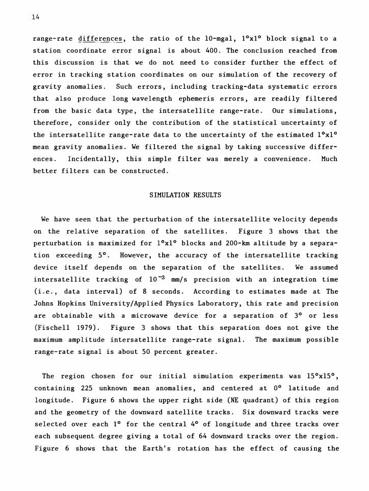
mean gravity anomalies. We filtered the signal by taking successive differ­

ences. Incidentally, this simple filter was merely a convenience. Much

better filters can be constructed.

SIMULATION RESULTS

We have seen that the perturbation of the intersatellite velocity depends

on the relative separation of the satellites. Figure 3 shows that the

perturbation is maximized for lOxlo blocks and 200-km altitude by a separa­

tion exceeding 5°. However, the accuracy of the intersatellite tracking

device itself depends on the separation of the satellites. We assumed

intersatellite tracking of lO -3 mm/s precision with an integration time

(i. e., data interval) of 8 seconds. According to estimates made at The

Johns Hopkins University/Applied Physics Laboratory, this rate and precision

are obtainable with a microwave device for a separation of 3° or less

(Fischell 1979). Figure 3 shows that this separation does not give the

maximum amplitude intersatellite range-rate signal.

range-rate signal is about 50 percent greater.

The maximum possible

The region chosen for our initial simulation experiments was l5°xl5°,

containing 225 unknown mean anomalies, and centered at 0° latitude and

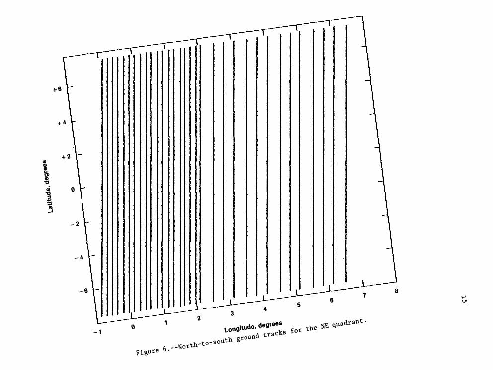
longitude. Figure 6 shows the upper right side (NE quadrant) of this region

and the geometry of the downward satellite tracks. Six downward tracks were

selected over each 1° for the central 4° of longitude and three tracks over

each subsequent degree giving a total of 64 downward tracks over the region.

Figure 6 shows that the Earth's rotation has the effect of causing the

+6

+4

+2 en Gl Gl .. � .., Ii 0 .., .a .,;:: j

-2

-4

-6 7

6

1 2 3

4 5

-1 o long\\ude. degrees

figure 6. __ North-to-south ground tracks for the NE quadrant.

8 l-" \}'I

16

ground tracks of the polar orbiting satellite to be slightly inclined to a

meridian. Note that the right edge of the region is carried away from the

tracks, resulting in poor sampling. This is one of the reasons our results

are valid only for the central area of the lSoxlSo region.

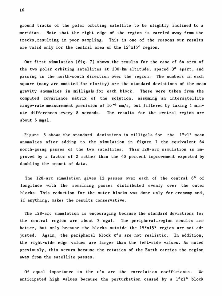
Our first simulation (fig. 7) shows the results for the case of 64 arcs of

the two polar orbiting satellites at 200-km altitude, spaced 3° apart, and

passing in the north-south direction over the region. The numbers in each

square (many are omitted for clarity) are the standard deviations of the mean

gravity anomalies in milligals for each block. These were taken from the

computed covariance matrix of the solution, assuming an intersatellite

range-rate measurement precision of 10-3 mm/s, but filtered by taking 1 min-

ute differences every 8 seconds.

about 6 mgal.

The results for the central region are

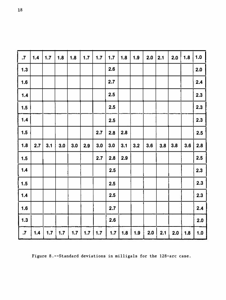
Figure 8 shows the standard deviations in mi11iga1s for the 1°x1° mean

anomalies after adding to the simulation in figure 7 the equivalent 64

north-going passes of the two satellites. This 128-arc simulation is im­

proved by a factor of 2 rather than the 40 percent improvement expected by

doubling the amount of data.

The l28-arc simulation gives 12 passes over each of the central 6° of

longitude with the remaining passes distributed evenly over the outer

blocks. This reduction for the outer blocks was done only for economy and,

i f anything, makes the results conservative.

The 128-arc simulation is encouraging because the standard deviations for

the central region are about 3 mgal. The peripheral-region results are

better, but only because the blocks outside the lSox15° region are not ad­

justed. Again, the peripheral block a's are not realistic. In addition,

the right-side edge values are larger than the left-side values. As noted

previously, this occurs because the rotation of the Earth carries the region

away from the satellite passes.

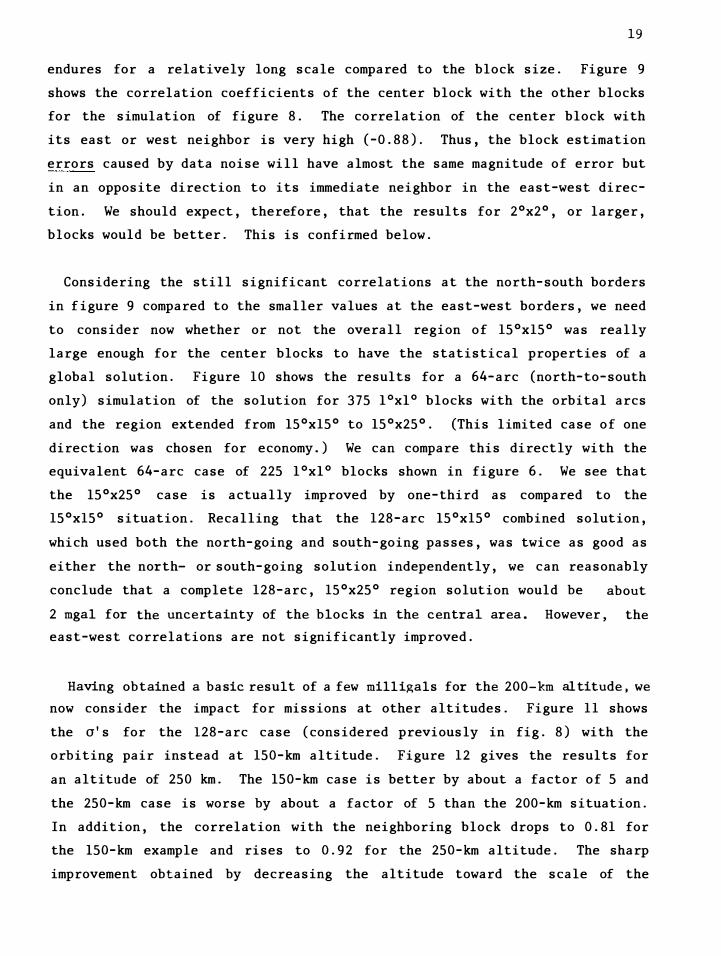
Of equal importance to the a's are the correlation coefficients. We

anticipated high values because the perturbation caused by a 1 °xl ° block

2.3 5.0 7.1 7.4 7.3 7.1 7.1 7.2 3.6 8.0 8.5 9.3 10.0 10.6

3.1 6.6

3.3 5.4

2.8 5.5

3.2 5.0

2.8 5.4 5.4 5.5 5.7 6.0

3.4 6.3 6.2 6.2 6.5 6.9

3.8 6.4 6.6 7.2 6.7 6.4 6.4 6.4 6.6 7.0 7.6 8.1 8.4 9.1

3.4 5.4 5.3 5.3 5.5 5.8

3.0 6.1 6.1 6.1 6.3 6.7

2.7 4.6

2.7 5.1

2.9 5.5

2.6 4.8

1.3 2.5 3.2 3.3 3.2 3.1 3.1 3.1 3.2 3.4 3.6 4.1 4.1 4.0

Figure 7. --Standard deviations in milligals for IOxlo mean anomalies with 64 north-to-south satellite tracks.

17

7.9

7.8

7.0

6 .3

6.6

6.1

7.4

7.7

6.3

7.2

5.2

6.2

6.4

4.6

2.8

18

.7 1.4 1.7 1.8 1.8 1.7 1.7 1.7 1.8 1.9 2.0 2.1 2.0 1.8 1.0

1.3 2.6 2.0

1.6 2.7 2.4

1.4 2.5 2.3

1.5 2.5 2.3

1.4 2.5 2.3

1.5 2.7 2.8 2.8 2.5

1.8 2.7 3.1 3.0 3.0 2.9 3.0 3.0 3.1 3.2 3.6 3.8 3.8 3.6 2.8

1.5 2.7 2.8 2.9 2.5

1.4 2.5 2.3

1.5 2.5 2.3

1.4 2.5 2.3

1.6 2.7 2.4

1.3 2.6 2.0

.7 1.4 1.7 1.7 1.7 1.7 1.7 1.7 1.8 1.9 2.0 2.1 2.0 1.8 1.0

Figure 8. --Standard deviations in milligals for the 128-arc case.

19

endures for a relatively long scale compared to the block size. Figure 9

shows the correlation coefficients of the center block with the other blocks

for the simulation of figure 8. The correlation of the center block with

its east or west neighbor is very high (-0. 88). Thus, the block estimation

errors caused by data noise will have almost the same magnitude of error but

in an opposite direction to its immediate neighbor in the east-west direc­

tion. We should expect, therefore, that the results for 2°x2°, or larger,

blocks would be better. This is confirmed below.

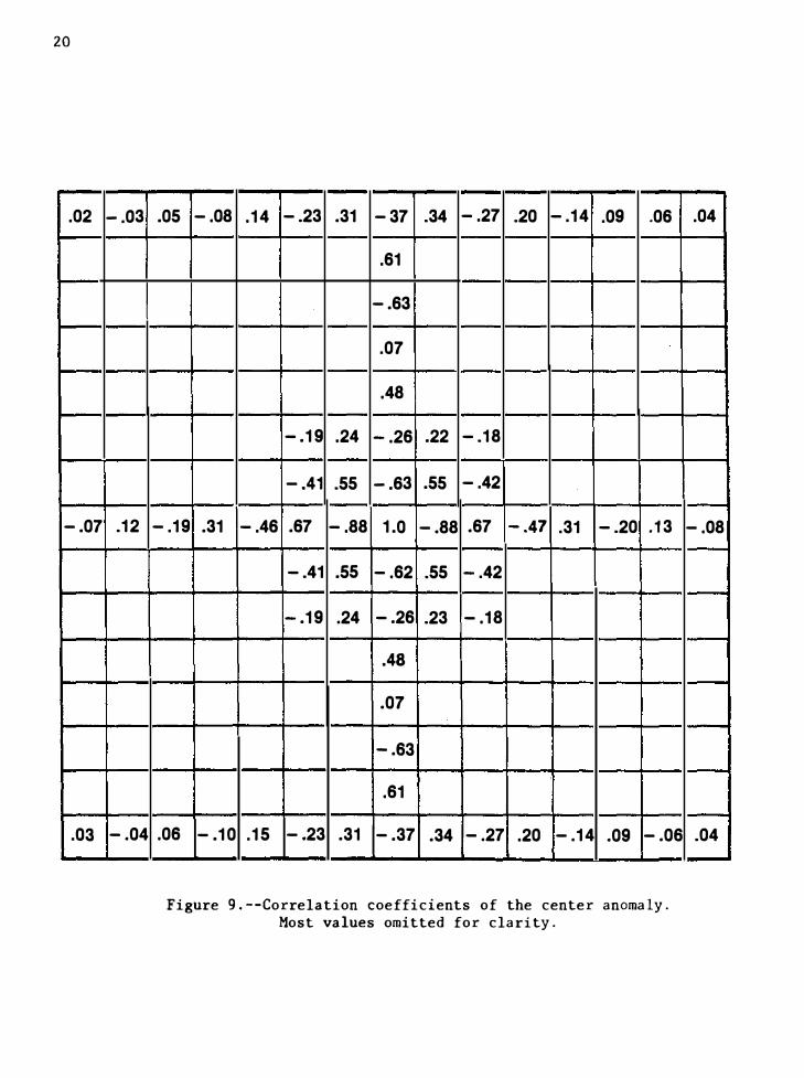
Considering the still significant correlations at the north-south borders

in figure 9 compared to the smaller values at the east-west borders, we need

to consider now whether or not the overall region of 15°x15° was really

large enough for the center blocks to have the statistical properties of a

global solution. Figure 10 shows the results for a 64-arc (north-to-south

only) simulation of the solution for 375 lOxlo blocks with the orbital arcs

and the region extended from l5°x15° to l5°x25°. (This limited case of one

direction was chosen for economy.) We can compare this directly with the

equivalent 64-arc case of 225 lOxlo blocks shown in figure 6. We see that

the l5°x25° case is actually improved by one-third as compared to the

15°x15° situation. Recalling that the 128-arc l5°x15° combined solution,

which used both the north-going and south-going passes, was twice as good as

ei ther the north- or south-going solution independently, we can reasonably

conclude that a complete 128-arc, 15°x25° region solution would be about

2 mgal for the uncertainty of the blocks in the central area. However, the

east-west correlations are not significantly improved.

Having obtained a basic result of a few milligals for the 200-km altitude, we

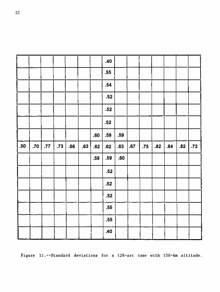
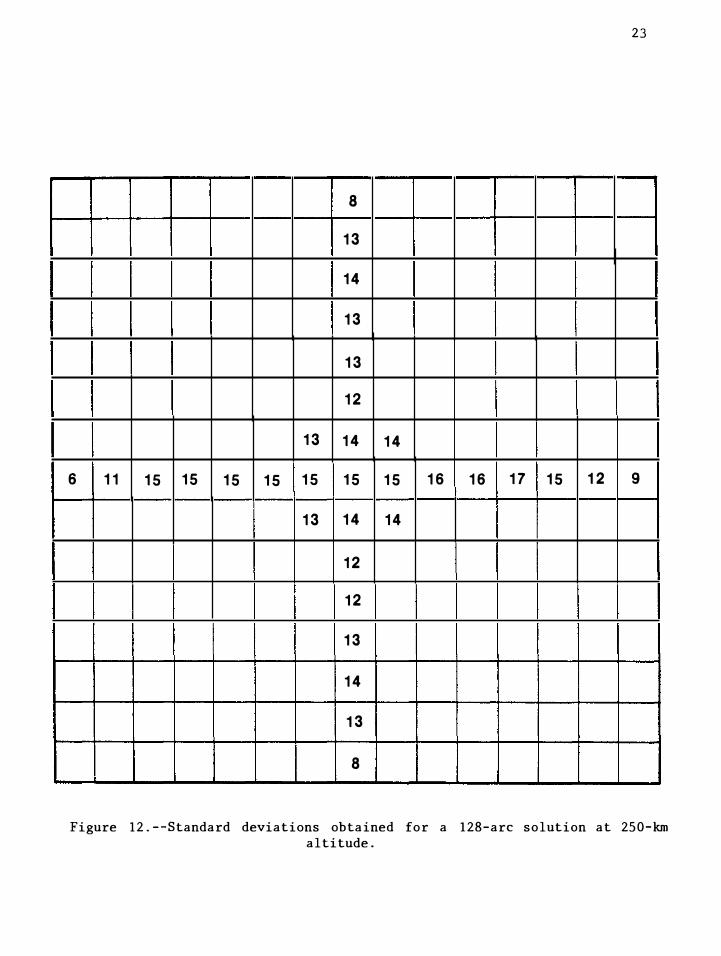
now consider the impact for missions at other altitudes. Figure 11 shows

the a's for the 128-arc case (considered previously in fig. 8) with the

orbiting pair instead at 150-km altitude. Figure 12 gives the results for

an altitude of 250 km. The l50-km case is better by about a factor of 5 and

the 250-km case is worse by about a factor of 5 than the 200-km situation.

In addition, the correlation with the neighboring block drops to 0. 81 for

the l50-km example and rises to 0. 92 for the 250-km altitude. The sharp

improvement obtained by decreasing the altitude toward the scale of the

20

.02 -.03 .05 -.08 .14 -.23 .31 -37 .34 -.27 .20 -.14 .09 .06 .04

.61

-.63

.07

.48

-.19 .24 -.26 .22 -.18

-.41 .55 -.63 .55 -.42

-.07 .12 -.19 .31 -.46 .67 -.88 1.0 -.88 .67 -.47 .31 -.20 .13 -.08

-.41 .55 -.62 .55 -.42

-.19 .24 -.26 .23 -.18

.48

.07

-.63

.61

.03 -.04 .06 -.10 .15 -.23 .31 -.37 .34 -.27 .20 -.14 .09 -.06 .04

Figure 9.--Correlation coefficients of the center anomaly. Most values omitted for clarity.

2.5

4.0

4.2

4.0

3.8

4.0

4.1

4.2

4.1

4.1

4.2

3.9 4.0 4.6

2.1 4.1 5.3 5.5 5.2 4.6 4.1 4.3 5.1 6.0 7.1 7.9 8.4 8 .5 7.1

4.1 4.2 4.9

4.2

4.2

4.3

4.5

4.7

4.0

3.8

4.3

4.2

4.3

2.9

Figure 10.--Standard deviations obtained for a 15°x25° solution with 64 north-south passes.

21

22

.40

.55

.54

.52

.52

.52

.60 .59 .59

.50 .70 .77 .73 .66 .63 .62 .62 .63 .67 .75 .82 .84 .82 .73

.59 .59 .60

.52

.52

.52

.55

.55

.40

Figure 1 1. --Standard deviations for a 128-arc case with ISO-km altitude.

23

8

13

14

13

13

12

13 14 14

6 11 15 15 15 15 15 15 15 16 16 17 15 12 9

13 14 14

12

12

13

14

13

8

Figure 12. --Standard deviations obtained for a 128-arc solution at 2S0-km altitude.

24

IOx IO blocks (-Ill km/deg at the surface) tends to confirm Schwarz's ( 1971)

rule that the horizontal resolution of the low-low satellite experiment is

approximately equal to the altitude of the orbiting pair.

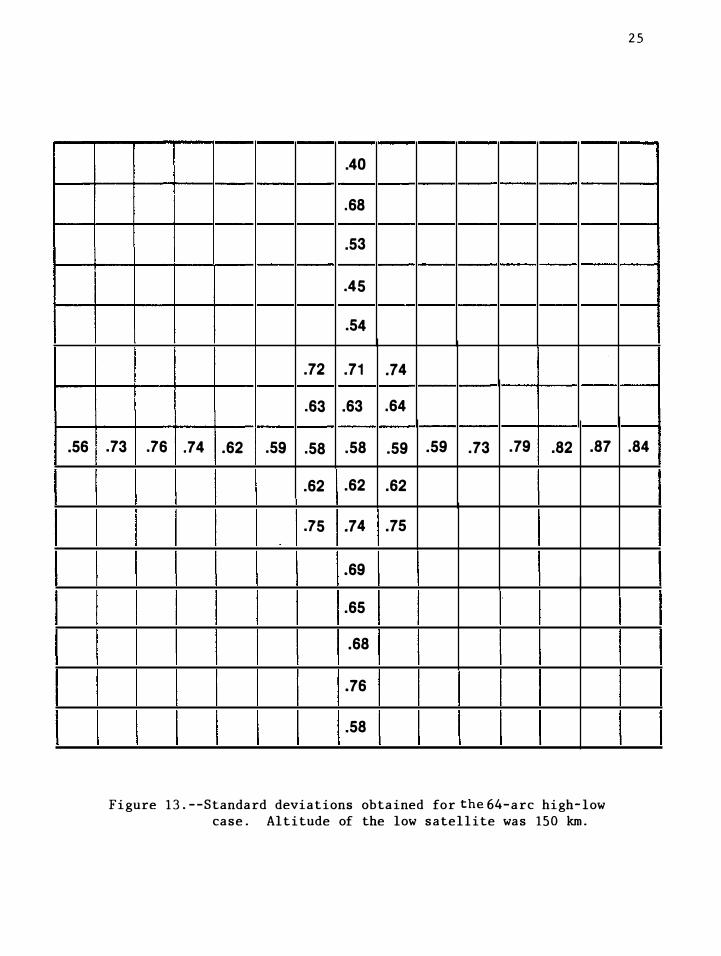
Our final consideration was the possible performance of a so-called

"high-low" system where one of the satellites is geosynchronous. Several

advantages of this method have been alleged. Indeed, for a given intersatel­

lite speed measurement specification, the high-low case should be superior

overall because, for blocks away from the Equator, both the horizontal and

vertical components of the intersatellite velocity perturbation are observed.

Figure 13 gives the results obtained for a 64-arc case (south-going passes

alone) with the geosynchronous member of the pair placed directly over the

center of the lSoxlSo region and the low satellite at lSO-km altitude. Com­

parison with figure 10 shows that this high-low configuration of 64-arcs is

as effective as a l2B-arc low-low experiment with all else being equal. But

we emphasize these results depend entirely on intersatellite range-rate

measurements of 10-3 mm/s precision. This precision appears to be obtainable

with laser interferometric or sophisticated microwave devices for satellites

orbiting close to each other, but probably further technological development

is required for observations to a geosynchronous satellite instead of an­

other near-Earth one.

It is interesting to compute the results obtainable when the block size is

changed to 2°x2°. I f the IOxlo block errors were uncorrelated, mean 2°x2°

anomalies would have a standard deviation of \ of the I °x I ° anomalies

comprising them. However, because of the large negative correlation of ad­

jacent blocks, 2°x2° mean anomalies have a precision of 0.29 mgal, an im­

provement of 10 compared to the 1 °xl ° case. Because the 200-km altitude

corresponds almost exactly to the dimension of a 2°x2° block, this result

provides another demonstration of Schwarz's rule.

DISCUSSION

It would be desirable to be able to give a firm number for the capability

of an intersatellite tracking mission to determine the geopotential, but our

.56

.40

.68

.53

.45

.54

.72 .71 .74

.63 .63 .64

.73 .76 .74 .62 .59 .58 .58 .59 .59 .73 .79 .82 .87

.62 .62 .62

.75 .74 .75

.69

.65

.68

.76

.58

Figure 13.--Standard deviations obtained for the 64-arc high-low case. Altitude of the low satellite was 150 km.

25

.84

26

study did not achieve this. However, from a conservative viewpoint we be­

lieve that we have answered an important question: Is the capability o f

satellite-to-satellite tracking for determining the geopotential at the

10xlo-resolution level near 10 mgal or 1 mgal? Our answer is the latter,

especially because our simulations were so conservative. For example, the

number of passes over the blocks in our simulation would be attained in a

real mission in about 4 months. Much longer missions are within the capa­

bility o f surface-force compensation systems, so better results could be

expected from longer missions. In addition, a somewhat lower altitude could

be chosen. Recall that dropping from 200 km to 150 km caused a five-fold

improvement. An intermediate altitude choice o f about 180 km, rather than

200 km, could result in a substantial improvement, but at the cost of a 50

percent increase in atmospheric drag force. Improvements are also possible

in intersatellite measurement capabilities. This would enable an increase

in the intersatellite separation and would improve the signal/ noise for the

experiment. Finally, a careful inclusion o f a priori information taken from

the vast store of existing geopotential data would improve the situation.

Thus, it seems apparent that a suitably optimized 1 year low-low satellite

mission could produce mean anomalies at the l-mgal level o f precision. The

high correlations in the east-west direction are unfortunately large, but

are tolerable because the a's are so small compared to the actual variation

o f gravity anomalies (about 30 mgal rms in lOxlo blocks).

Some remarks should be made on the significance of a global lOxlo precise

gravity field. Such a field does not necessarily produce an ocean geoid

suitable as a reference surface for satellite altimetry at the 1° wavelength.

Chovitz (1973) showed that Kaula' s (1966) rule-of-thumb 10-5/.£2 for the

degree variances o f geopotential coefficients implies unaccounted-for geoid

undulations of 64/.£ meters for a geoid computed to degree .£. For a lOxlo

solution, the undulations shorter than 1° could be about 30 cm. At wave­

lengths longer than 1°, the geoid obtained from lOxlo mean anomalies would

be highly accurate. In addition, the existence o f a geopotential field

accurate up to the lOxlo scale would effectively solve the problem of satel­

lite orbit determination. With such a field and a satellite equipped with a

27

surface-force compensation device, a satellite ephemeris accurate to better

than 10 cm could be obtained. Also, the computation of gravimetric geoids

such as the one by Marsh and Chang (1978 ) , now widely used as a reference

surface for satellite altimetry, could be improved because the effects o f

mean anomalies in regions distant from a geoid computation point would be

accurately known. Finally, a global 1 °xl 0 field would be of interest to

geophysicists.

ACKNOWLEDGMENT

This research was partially funded by the National Aeronautics and Space

Administration, Washington, D. C., under purchase order no. S59873B. The

The authors benefited from conversations with Prof. R. Rapp of Ohio State

University.

28

REFERENCES

Argentiero, P. and Lowrey, B. , 1978: A comparison of satellite systems for gravity field measurements, Geophysical Surveys, 3, 207-223.

Belousov, S. L. , 1962: Tables of Normalized Associated Legendre Polynomials. The Macmillan Company, New York, (translated from Russian by D. E. Brown), 1-14.

Chovitz, B. , 1973: Downward continuation of the potential from satellite altitudes, Boll. Geod. Sci. Affini, 32, 81-88.

Chovitz, B. , Lucas, J. , and Morrison, F. , 1973: Gravity gradients at satellite altitudes. NOAA Technical Report NOS 59, National Ocean Survey, National Oceanic and Atmospheric Administration, Rockville, Md. , 24 pp.

Fischell, R. (The John Hopkins University/Applied Physics Laboratory, Silver Spring, Md.), 1979 (personal communication).

Giacaglia, G. E. O. and Lundquist, C. A. , 1972: Sampling Functions for Geophysics. Smithsonian Astrophysical Observatory Special Report 344, Cambridge, Mass.

Hotine, M. and Morrison, F. , 1969: First integrals of the equations of satellite motion, Bulletin Geodes ique,No. 91, 41-45.

Kaula, W. M. , 1963: The investigation of the gravitational fields of the moon and planets with artificial satellites, Advan. Space Sci. Technol. , 5, 210-226.

Kaula, W. M. , Cherubim, G. , Burkhand, N. , and Jackson, D. D. , 1978: Application of inverse theory to new satellite systems for determination of the gravity field. Report No. AFGL-TR-78-0073, U. S. Air Force, Hanscomb Air Force Base, MA 01731.

Koch, K. R. and Witte, B. , 1971: Earth's gravity field represented by a simple layer potential from Doppler tracking of satellites, J. Geophys. Res. , 76, 8471-8479.

Marsh, J. G. and Chang, E. S. , 1976: Detailed gravimetric geoid confirma­tion of sea surface topography detected by the Skylab S-193 altimeter in the Atlantic Ocean, Bulletin Geodesique, No. 50, 29 1-299.

Moritz, H. , 1978: Least-squares collocation, Reviews of Geophysics and Space Physics, 16, 421-430.

Morrison, F. (National Geodetic Survey, NOS/NOAA, R k '11 Md ) 1979 oc V1 e, . (paper in preparation).

29

Morrison, F. , 1977: Algorithms for computing the geopotential using a simple-layer density model. NOAA Technical Report NOS 67 NGS 3. National Ocean Survey, National Oceanic and Atmospheric Administration, Rockville, Md. , 41 pp.

Morrison, F., 1976: Algorithms for computing the geopotentia1 using a simple layer density model, J. Geophys. Res., 81, 4933-4936.

Orlin, H. , 1959: The three components of the external anomalous gravity field, J. Geophys. Res. , 64, 2393-2399.

Rapp, R. H. , 1979: GEOS 3 data processing for the recovery of geoid undu­lations and gravity anomalies, J. Geophys. Res., 84, 3784-3792.

Schwarz, C. R., 1972: Refinement of the gravity field by satellite-to­satellite Doppler tracking, Geophysical Monograph, 15, American Geophysical Union, Washington, D. C.

Wolff, M. ,1969: Direct measurements of the Earth's gravitational potential using a satellite pair, J. Geophys. Res. , 74, 5295-5300.

<Continued from inside front cover)

NOS NGS-3 Adjustment of geodetic field data using a sequential method. Marvin C. Whiting and Allen J. Pope, Ma rch 1976, 11 pp (PB253967). A sequential adjustment is adopted for use by NGS field parties.

NOS NGS-4 Reducing the profile of sparse symmetric matrices. Richard A. Snay, June 1976, 24 pp (PB-258476). An algorithm for improving the profile of a sparse symmetric matrix is introduced and tested against the widely used reverse CUthill-McKee algorithm.

NOS NGS-5 National Geodetic Survey data: availability, explanation, and application. Joseph F . Dracup, June 1976, 4 5 p p (PB258475). The summary gives data and services available from from NGS. accuracy of surveys, and uses of specific data.

NOS NGS-6 Determination of North American Datum 1983 coordinates of map corners. T. Vincenty. October 1976, 8 pp (PB262442). Predictions of changes in coordinates of map corners are detailed.

NOS NGS-7 Recent elevation change in Southern California. S.R. Holdahl. February 1977, 19 pp (PB265-940). Velocities of elevation change were determined from Southern Calif. leveling data for 1906-62 and 1959-76 epochs.

NOS NGS-8 Establishment of calibration base lines. Joseph F. Dracup, Charles J. Fronczek, and Raymond W. Tomlinson, August 1977, 22 pp (PB277130). Specifications are given for establishing cali­bration base lines.

NOS NGS-9 National Geodetic Survey publications on surveying and geodesy 1976. September 1977, 17 pp (PB275l8l). Compilation lists publications authored by NGS staff in 1976, source availa­bility for out-of-print Coast and Geodetic Survey publications, and subscription information on the Geodetic Control Data Automatic Mailing List.

NOS NGS-IO Use of calibration base lines. Charles J. Fronczek, December 1977, 38 pp (PB279574). De­tailed explanation allows the user to evaluate electromagnetic distance measuring instru­ments.

NOS NGS-ll Applicability of array algebra. Richard A. Snay, February 1978, 22 pp (PB281196). Condi­tions required for the transformation from matrix equations into computationally more effi­cient array equations are considered.

NOS NGS-12 The TRAV-lO horizontal network adjustment program. Charles R. Schwarz, April 1978, 52 pp (PB283087). The design, objectives. and specifications of the horizontal control adjustment program are presented.

NOS NGS-13 Application of three-dimensional geodesy to adjustments of horizontal networks. T. Vincenty and B. R. Bowring. June 1978. 7 pp (PB286672). A method is given for adjusting measurements in three-dimensional space without reducing them to any computational surface.

NOS NGS-14 Solvability analysis of geodetic networks using logical geometry. Richard A. Snay, October 1978, 29 pp (PB291286). No algorithm based solely on logical geometry has been found that can unerringly distinguish between solvable and unsolvable horizontal networks. For leveling networks such an algorithm is well known.

NOS NGS-15 Goldstone validation survey - phase 1. William E. Carter and James E. Pettey, November 1978, 44 pp (PB2923l0). Results are given for a space system validation study conducted at the Goldstone, Calif., Deep Space Communication Complex.

NOS NGS-16 Determination of North American Datum 1983 coordinates of map corners (Second Prediction). T. Vincenty, April 1979, 6 pp (PB297245). New predictions of changes in coordinates of of map corners are given.

NOS NGS-17 The HAVAGO three-dimensional adjustment program. T. Vincenty. May 1979. 18 pp (PB297069). The HAVAGO computer program adjusts numerous kinds of geodetic observations for high preci­sion special surveys and ordinary surveys.

NOS NGS-18 Determination of astronomic positions for California-Nevada boundary monuments near Lake Tahoe. James E. Pettey, March. 1979. 22 pp (PB301264). Astronomic observations of the 120th meridian were made at the request of the Calif. State Lands Commission.

NOS NGS-19 HOACOS: A program for adjusting horizontal networks in three dimensions. T. Vincenty. July 1979, 18 pp (PB30l35l). Horizontal networks are adjusted simply and efficiently in the height-controlled spatial system without reducing observations to the ellipsoid.

NOS NGS-20 Geodetic leveling and the sea level slope along the California coast. Emery I. Balazs and Bruce C. Douglas, September 1979. 23 pp. Heights of four local mean sea levels for the 1941-59 epoch in California are determined and compared from five geodetic level lines observed (leveled) between 1968-78.

NOS NGS-2l Haystack-Westford Survey. W. E. Carter, C. J. Fronczek. and J. E. Pettey, September 1979, 57 pp. A special purpose survey-was conducted for VLBI test comparison.

NOS -NGS-22 Gravimetric tidal loading computed from integrated Green1s functions. C. C. Goad. October 1979. 15 pp. Tidal loading is computed using integrated Green1s functions.

NOS NGS-23 Use of auxiliary ellipsoids in height-controlled spatial adjustments. B. R. Bowring and T. Vincenty. November 1979. 6 pp. Auxiliary ellipsoids are used in adjustments of networks in the height-controlled three-dimensional system for controlling heights and simplifying transformation of coordinates.

<Continued on inside back cover)

�.s. GOVERNMENT PRINTING OFFICE: 198{l 3IH146/364 1-1

NOS 65 NGS

NOS 66 NGS 2

NOS 67 NGS 3

NOS 68 NGS 4

NOS 7U NGS ;

NOS 71 NGS 6

NOS 72 NGS 7

NOS 73 NGS 8

NOS 74 NGS 9

(Continued)

NOAA Technical Reports, NOS/NGS subseries

The statistics of residuals and the detection of outliers. Allen J. Pope, May 1976, 133 pp (PB2S8428). A criterion for rejection of bad geodetic data is derived on the basis of residuals from a simultaneous least-squares adjustment. Subroutine TAURE is included. Effect of Geoceiver observations upon the classical triangulation network. R. E. Moose and S. W. Henriksen, June 1976, 65 pp (PB260921). The use of Geoceiver observations is investigated as a means of improving triangulation network adjustment results. Algorithms for computing the geopotential using a simple-layer density model. Foster Morrison, March 1977, 41 pp {PB266967). Several algor1thms are developed for computing with high accuracy the gravitational attraction of a simple-density layer at arbitrary altitudes. Computer program is included. Test results of first-order class III leveling. Charles T. Whalen and Emery Balazs, No­vember 1976, 30 pp (GPO# 003-017-00393-1) (PB265421). Specifications for releveling the National vertical control net were tested and the results published. Selenocentric geodet1c reterence system. Frederick J. Doyle, Atef A. Elassal, and James R. Lucas, February 1977, 53 pp (PB266046). Reference system was established by simulta­neous adjustment of 1,233 metric-camera photographs of the lunar surface from which 2,662 terrain points were positioned. Application of digital filtering to satellite geodesy. C. C. Goad, May 1977, 73 pp (PB-270192). Variations in the orbit of GEOS-3 were analyzed for Mz tidal harmonic co­ettic1ent values which perturb the orbits of artificial satellites and the Moon. Systems for the determination of polar motion. Soren W. Henriksen, May 1977, 55 pp (PB274698). Methods for determining polar motion are described and their advantages and disadvantages compared. Control leveling. Charles T. Whalen, May 1978, 23 pp (GPO# 003-017-00422-8) (PB286838). The history of the National network of geodetic control, from its origin in 1878, is pre­sented in addition to the latest observational and computational procedures. Survey of the McDonald Observatory radial line scheme by relative lateration techniques. William E. Carter and T. Vincenty, June 1978, 33 pp (PB287427). Results of experimental application of the "ratio method" of electromagnetic distance measurements are given for high resolution crustal deformation studies in the vicinity of the McDonald Lunar Laser Ranging and Harvard Radio Astronomy Stations.

NOS 75 NGS 10 An algorithm to compute the eigenvectors of a symmetric matrix. E. Schmid, August 1978, 'pp (PB287923). Method describes computations tor eigenvalues and eigenvectors of a symmetric matrix.

NOS 76 NGS 11 The application of multiquadric equations and point mass anomaly models to crustal move­ment studies. Rolland L. Hardy, November 1978, 63 pp (PB293544). Multiquadric equa­tions, both harmonic and nonharmonic, are suitable as geometric prediction functions for surface deformation and have potentiality for usage in analysis of subsurface mass redis­tribution associated with crustal movements.

NOS 79 NGS 12 Optimization of horizontal control networks by nonlinear programing. Dennis G. Hilbert, August 1979, 44 pp. Several horizontal geodetic control networks are optimized at mini­mum cost while mainta1ning des1red accuracy standards.

NOS NGS

NOAA Manuals, NOS/NGS sub series

Geodetic bench marks. Lt. Richard P. Floyd, September 1978, 56 pp (GPO# 003-017-00442-2) (P8296427). Reference guide provides specifications for highly stable bench marks, including chapters on installation procedures, vertical instability, and site selection considerations.

u.s. DEPARTMENT OF COMMERCE National Oceanic and Atmospheric Administration National Ocean Survey National Geodetic Survey, C 1 3x4 Rockville, Maryland 20852

OFFICIAL BUSINESS

NOAA- -S!T 80- 26

POSTAGE AND FEES PAID � U.S DEPARTMENT OF COMMERCE �

COM-2 1 0 U.S.MAIL

PR I NTED MATTER ®