NOAA Technical Memorandum ERL PMEL-12

A SHALLOW WATER PRESSURE-TEMPERATURE GAGE (PTG):

DESIGN, CALIBRATION, AND OPERATION

Stanley P. HayesJohn GlennNancy N. Soriede

Pacific Marine Environmental LaboratorySeattle, WashingtonJune 1978

UNITED STATESDEPARTMENT OF COMMERCE

JUlnitl M. Kreps, Secretlry

NATIONAL OCEANIC ANDATMOSPHERIC ADMINISTRATION

Richard A. Frank, Administrator

Environmental Researchlaboratones

Wilmot N. Hess, Director

DISCLAIMER

The NOAA Environmental Research Laboratories does not approve, recom­mend, or endorse any proprietary product or proprietary material mentionedin this publication. No reference shall be made to the NOAA EnvironmentalResearch Laboratories, or to this publication furnished by the NOAA Envi­ronmental Research Laboratories, in any advertising or sales promotionwhich would indicate or imply that the NOAA Environmental Research Labora­tories approves, recommends, or endorses any proprietary product or propri­etary material mentioned herein, or which has as its purpose an intent tocause directly or indirectly the advertised product to be used or purchasedbecause of this NOAA Environmental Research Laboratories publication.

i i

CONTENTS

Page

LIST OF FIGURES iv

ABSTRACT 1

l. INTRODUCTION 1

2. INSTRUMENT DESIGN 3

3. CALIBRATION 8

4. DATA PROCESSING 19

5. SAMPLE RESULTS 21

6. REFERENCES 31

iii

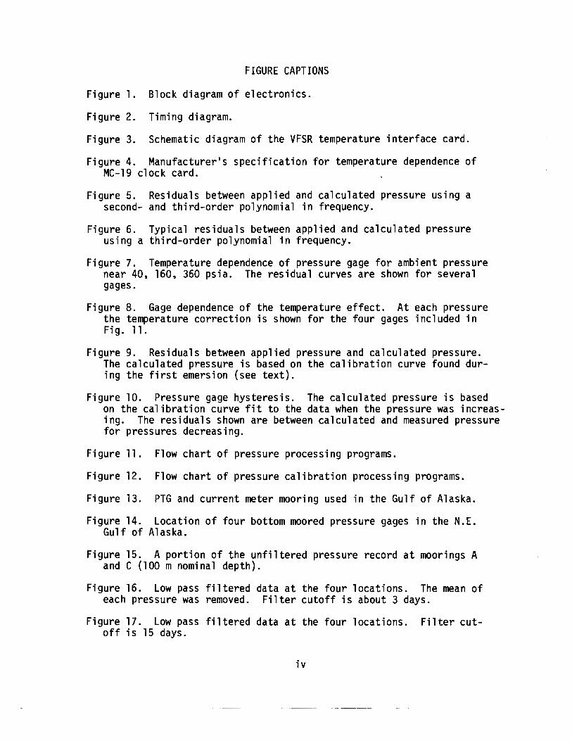
FIGURE CAPTIONS

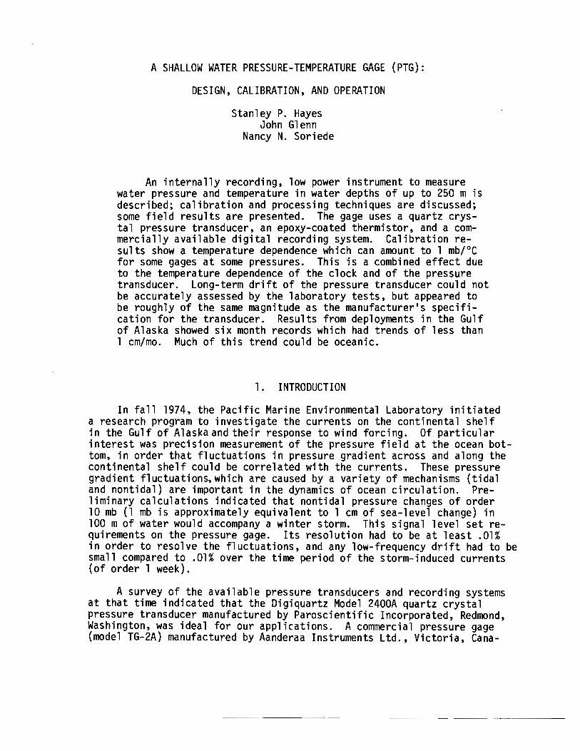
Figure 1. Block diagram of electronics.

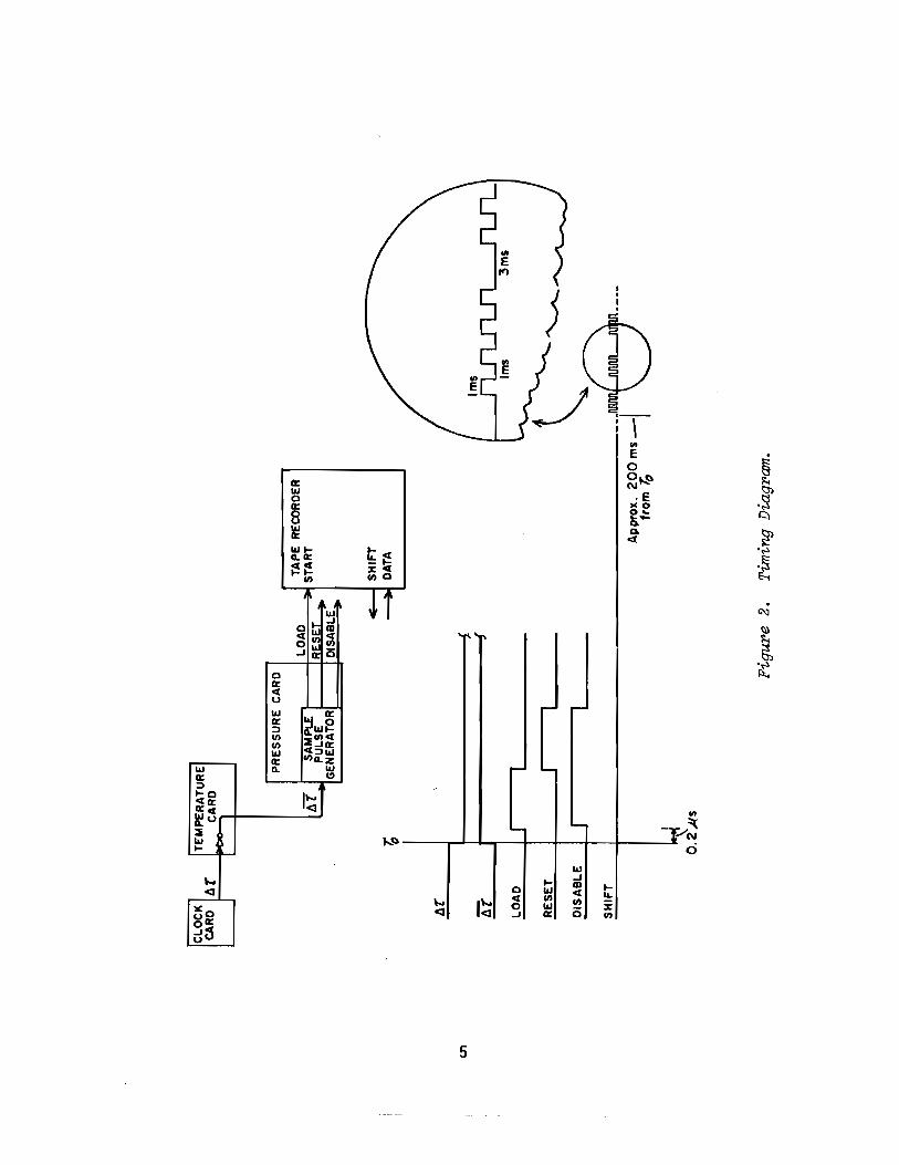
Figure 2. Timing diagram.

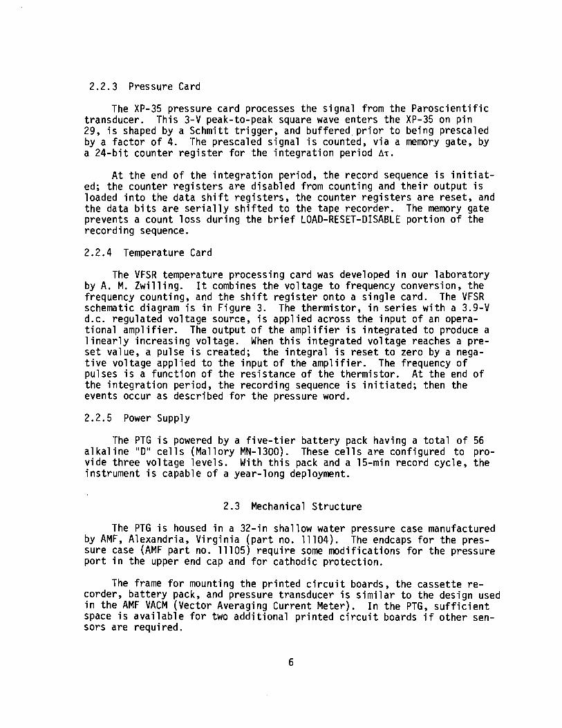
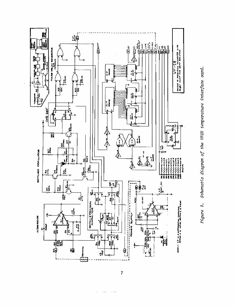
Figure 3. Schematic diagram of the VFSR temperature interface card.

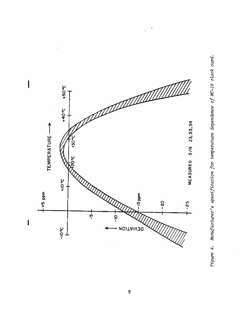
Figure 4. Manufacturer's specification for temperature dependence ofMC-19 clock card.

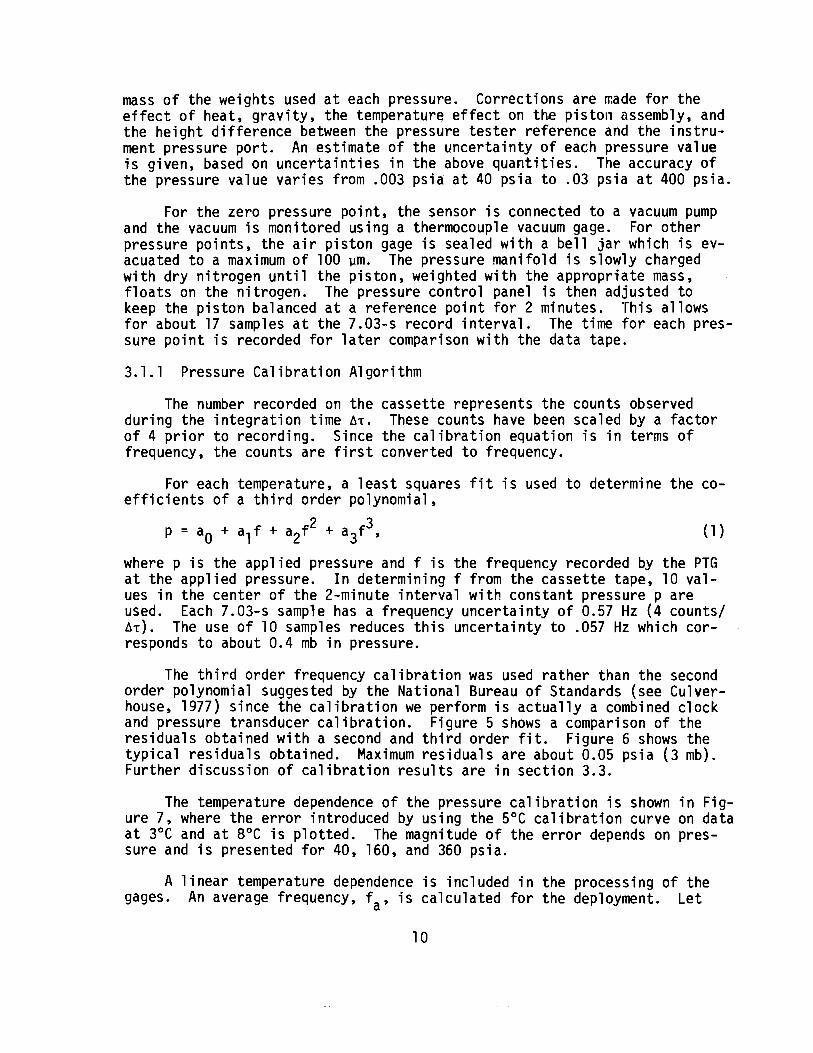
Figure 5. Residuals between applied and calculated pressure using asecond- and third-order polynomial in frequency.

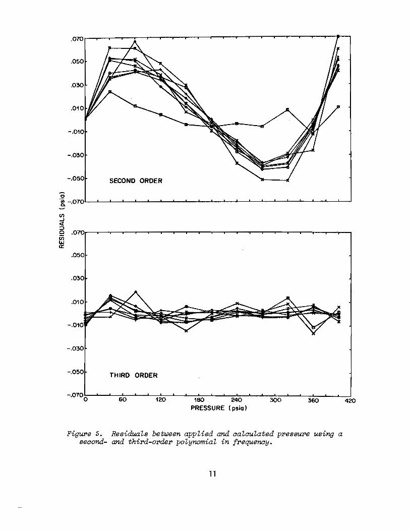
Figure 6. Typical residuals between applied and calculated pressureusing a third-order polynomial in frequency.

Figure 7. Temperature dependence of pressure gage for ambient pressurenear 40, 160, 360 psia. The residual curves are shown for severalgages.

Figure 8. Gage dependence of the temperature effect. At each pressurethe temperature correction is shown for the four gages included inFig. 11.

Figure 9. Residuals between applied pressure and calculated pressure.The calculated pressure is based on the calibration curve found dur­ing the first emersion (see text).

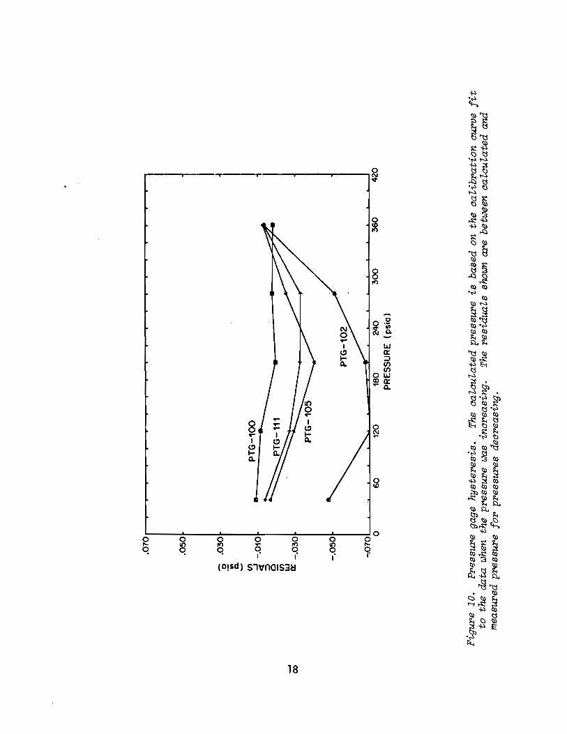
Figure 10. Pressure gage hysteresis. The calculated pressure is basedon the calibration curve fit to the data when the pressure was increas­ing. The residuals shown are between calculated and measured pressurefor pressures decreasing.

Figure 11. Flow chart of pressure processing programs.

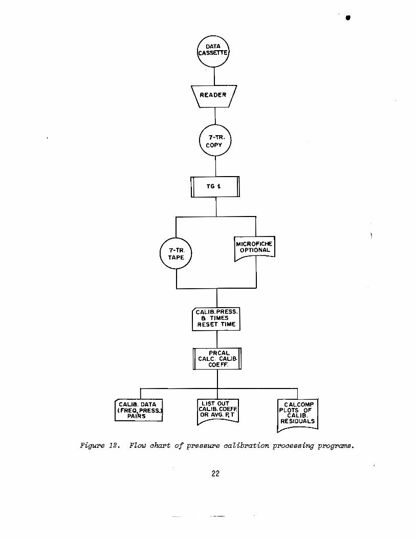
Figure 12. Flow chart of pressure calibration processing programs.

Figure 13. PTG and current meter mooring used in the Gulf of Alaska.

Figure 14. Location of four bottom moored pressure gages in the N.E.Gulf of Alaska.

Figure 15. A portion of the unfiltered pressure record at moorings Aand C (100 m nominal depth).

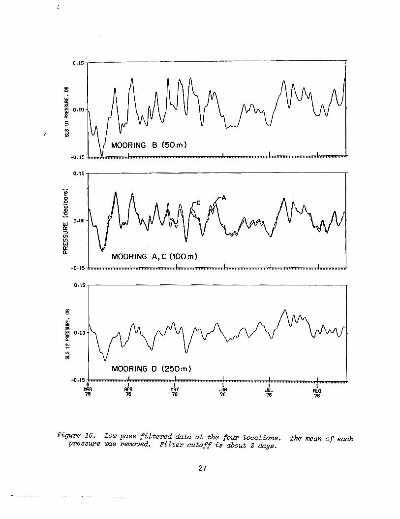
Figure 16. Low pass filtered data at the four locations. The mean ofeach pressure was removed. Filter cutoff is about 3 days.

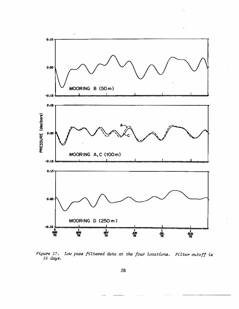
Figure 17. Low pass filtered data at the four locations. Filter cut­off is 15 days.

iv

A SHALLOW WATER PRESSURE-TEMPERATURE GAGE {PTG}:

DESIGN, CALIBRATION, AND OPERATION

Stanley P. HayesJohn Glenn

Nancy N. Soriede

An internally recording, low power instrument to measurewater pressure and temperature in water depths of up to 250 m isdescribed; calibration and processing techniques are discussed;some field results are presented. The gage uses a quartz crys­tal pressure transducer, an epoxy-coated thermistor, and a com­mercially available digital recording system. Calibration re­sults show a temperature dependence which can amount to 1 mb/oCfor some gages at some pressures. This is a combined effect dueto the temperature dependence of the clock and of the pressuretransducer. Long-term drift of the pressure transducer could notbe accurately assessed by the laboratory tests, but appeared tobe roughly of the same magnitude as the manufacturer's specifi­cation for the transducer. Results from deployments in the Gulfof Alaska showed six month records which had trends of less than1 cm/mo. Much of this trend could be oceanic.

1. INTRODUCTION

In fall 1974, the Pacific Marine Environmental Laboratory initiateda research program to investigate the currents on the continental shelfin the Gulf of Alaska and their response to wind forcing. Of particularinterest was precision measurement of the pressure field at the ocean bot­tom, in order that fluctuations in pressure gradient across and along thecontinental shelf could be correlated with the currents. These pressuregradient fluctuations,which are caused by a variety of mechanisms {tidaland nontidal} are important in the dynamics of ocean circulation. Pre­liminary calculations indicated that nontidal pressure changes of order10 mb {l mb is approximately equivalent to 1 cm of sea-level change} in100 mof water would accompany a winter storm. This signal level set re­quirements on the pressure gage. Its resolution had to be at least .01%in order to resolve the fluctuations, and any low-frequency drift had to besmall compared to .01% over the time period of the storm-induced currents{of order 1 week}.

A survey of the available pressure transducers and recording systemsat that time indicated that the Digiquartz Model 2400A quartz crystalpressure transducer manufactured by Paroscientific Incorporated, Redmond,Washington, was ideal for our applications. A commercial pressure gage{model TG-2A} manufactured by Aanderaa Instruments Ltd., Victoria, Cana-

----- ---- -------~----- -------- --

TEM

PERA

TURE

VF-

SRPR

ESSU

REX

P-35

CLO

CK

MC

-19

N

.,

,i§'LOA

OS

HIF

TLO

AD

SH

IFT

LOA

D

SH

IFT

RE

GIS

TE

RSI

DA

TAI

~SHIFT

RE

GIS

TE

RSI

...JS

HIF

TR

EG

ISTE

RSI

RE

ET

'121'

..-"

••1

20

RE

SE

TI 1

2--

---

--1

20

I'21

--

--

--

-12

0D

ATA

~C

OU

NT

ER

SI

~C

OU

NT

ER

SI

?C

OU

NT

ER

SI

II

7.5m

in

~~

SA

MP

LELO

AD

Ir-tD

IVID

ER

SI

PU

LS

E~DIVIDERS

IG

EN

~~

~rt'

RE

SE

T.....

..,...

.16

.384

tur.

j".

RE

G~

SH

AP

ER

ID

ISA

BLE

IOS

C.

I,....

.......,

II:

..:.

::;J

",,:-+

7.03

1ec

15m

inR

T~

DIG

IOU

AR

TZ

IT

RA

NS

DU

CE

RR

ES

ET

Lvcc

AT

SE

LEC

T1

TA

PE

RE

CO

RD

ER

SY

ST

EM

MO

DE

L61

0

DA

TA

i4-

SH

IFT

ST

AR

T

Fig

ure

1.B

Zoak

diag

l'CD

no

feZ

eatl

'oni

as.

da, which used the Digiquartz sensor was available in 1974. We chose notto utilize this gage since it did not record time or temperature on themagnetic tape. Instead, a pressure-temperature gage (PTG) was designedwhich utilized a Digiquartz pressure transducer, a thermistor bead, model44032, made by Yellow Springs Instrument Company, Yellow Springs, Ohio,and a Sea Data recording system manufactured by Sea Data Corporation,Newton, Massachusetts. Pressure measuring systems similar to the one dis­cussed here have been developed in several laboratories. A particularsystem has been described by Culverhouse (1977). Rather than repeat thedetails which can be found elsewhere, we will present the general operat­ing characteristics of the PTG with emphasis on its distinctive features.The system calibration, processing techniques, and several results willthen be discussed.

2. INSTRUMENT DESIGN

2.1 Sensors

2. 1.1 Pressure

The instrument utilizes the model 2400A Digiquartz pressure trans­ducer mounted "in a model 300 shock mount. Full information on this trans­ducer is available from the manufacturer and in the article by Paros(1976). In brief, the transducer is a quartz crystal oscillator with afrequency which varies with applied pressure. The nominal frequency rangeis 40 kHz (0 psia) to 36 kHz (400 psia). The transducer requires low power(about 800 ~A). The manufacturer specifies a long-term drift rate of bet­ter than .01% per year. The transducer is connected to the ocean via anoil-filled nylon tube. The tube and transducer are filled with Dow Corn­ing silicone oil using a vacuum technique. The oil is in direct contactwith the seawater.

2.1.2 Temperature

The temperature measurements are made with a YSI model 44032 beadthermistor. These thermistors are calibrated in order to yield a preci­sion of .01oC. The thermistor is mounted adjacent to the pressure trans­ducer shock mount inside the PTG pressure case.

2.2 Electronics

A block diagram of the PTG electronics is shown in Figure 1. Thereare six printed circuit cards (all but the VFSR card are manufactured bySea Data Corp.) The data is recorded by a Sea Data model 610 four-trackdigital recorder which consist$ of a model 64E tape transport, CR-12 motordriver card, CR-21 head driver card, and CR-30 cassette control card. TheXP-35 pressure card, the VFSR temperature card, and the MC-19 clock cardmake up the remainder of the electronics. These components are describedbelow.

3

2.2.1 Recording Sequence

The Sea Data digital cassette recording system records 18 charactersduring each recording sequence. The order of the data words on the tapeis: two header characters. five characters (20 bits) of TIME data. sixcharacters (24 bits) of PRESSURE data. and five characters (20 bits) ofTEMPERATURE data.

The length of time that the pressure and temperature data are inte­grated is the ~~. preselected presently to be 7.03 s for calibration and15 min during deployment. Therefore. during deployment the data are inte­grated (counts stored) for 15 minutes. The data are then recorded. Thecounts which may occur during the brief recording time are saved so thatno count loss occurs.

A level change from the MC-19 clock card occurring at ~~ is sent tothe XP-35 pressure card where the sample pulse generator generates threesignals: LOAD. RESET. and DISABLE (Fig. 2).

The LOAD signal goes to the CR-30 cassette control card where it isseen as a RECORD REQUEST (START) and initializes the tape recording sys­tem.

The LOAD pulse also goes to the shift registers in the pressure. tem­erature. and clock processors. These registers will continue to followthe asynchronous parallel data bit inputs until the time when the LOADpulse decays; then the inputs from the counter registers are jammed intothe shift registers. At this time. RESET is generated which goes to allthe count registers in the pressure and temperature processors. and theregisters are all reset to 0.

During this time. DISABLE inhibits any further counts from passingthrough the pressure and temperature memory gates.

SHIFT pulses generated by the CR-21 head driver card are then sent inparallel to all shift registers where the data bits are serially shiftedthrough the registers to the CR-21 head driver PCB for recording. Theserial bit train is configured into 4-bit parallel characters for record­ing. The most significant bits are recorded first.

2.2.2 Clock Card

The MC-19 clock card initiates the recording sequence at preset inter­vals. The oscillator output is adjusted to be 16.384 kHz (61.03516 ~s per­iod) at 6°C (the nominal deployment temperature). The MC-19 provides forseveral divisions of the basic clock frequency. In general we use 7.03-sand 900-s record intervals for calibration and deployment. respectively.The TIME word generated by the MC-19 was chosen to update every 7.5 min inorder to be compatible with other instruments used in the laboratory.

4

CLO

CK

TE

MP

ER

AT

UR

EC

AR

D~r

CA

RD

PR

ES

SU

RE

CA

RD

LO

AD

TA

PE

RE

CO

RD

ER

~S

AM

PI£

IR

ES

ET

ST

AR

TP

ULS

EG

EN

ER

AT

OR

ID

ISA

BLE +

-S

HIF

T

~~

DA

TA

I

Af

()"I

~r

LO

AD

!!!!

UD

ISA

BL

E

!':H

IFT

o.~~

s

Fig

ure

2.

Tim

ing

Dia

gram

.

2.2.3 Pressure Card

The XP-35 pressure card processes the signal from the Paroscientifictransducer. This 3-V peak-to-peak square wave enters the XP-35 on pin29, is shaped by a Schmitt trigger, and buffered prior to being prescaledby a factor of 4. The prescaled signal is counted, via a memory gate, bya 24-bit counter register for the integration period ~T.

At the end of the integration period, the record sequence is initiat­ed; the counter registers are disabled from counting and their output isloaded into the data shift registers, the counter registers are reset, andthe data bits are serially shifted to the tape recorder. The memory gateprevents a count loss during the brief LOAD-RESET-DISABLE portion of therecording sequence.

2.2.4 Temperature Card

The VFSR temperature processing card was developed in our laboratoryby A. M. Zwilling. It combines the voltage to frequency conversion, thefrequency counting, and the shift register onto a single card. The VFSRschematic diagram is in Figure 3. The thermistor, in series with a 3.9-Vd.c. regulated voltage source, is applied across the input of an opera­tional amplifier. The output of the amplifier is integrated to produce alinearly increasing voltage. When this integrated voltage reaches a pre­set value, a pulse is created; the integral is reset to zero by a nega­tive voltage applied to the input of the amplifier. The frequency ofpulses is a function of the resistance of the thermistor. At the end ofthe integration period, the recording sequence is initiated; then theevents occur as described for the pressure word.

2.2.5 Power Supply

The PTG is powered by a five-tier battery pack having a total of 56al kal ine "0" cell s (Mallory MN-1300). These cell s are configured to pro­vide three voltage levels. With this pack and a 15-min record cycle, theinstrument is capable of a year-long deployment.

2.3 Mechanical Structure

The PTG is housed in a 32-in shallow water pressure case manufacturedby AMF, Alexandria, Virginia (part no. 11104). The endcaps for the pres­sure case (AMF part no. 11105) require some modifications for the pressureport in the upper end cap and for cathodic protection.

The frame for mounting the printed circuit boards, the cassette re­corder, battery pack, and pressure transducer is similar to the design usedin the AMF VACM (Vector Averaging Current Meter). In the PTG, sufficientspace is available for two additional printed circuit boards if other sen­sors are required.

6

f_r

c......,

~..,

I I {

VF

-SR

yo~rA"~

.,.F"'4~.""C"1~.N.~/lrR

..,.

,..a.

~Ir

C.I

I_r

AN

DSJN~r~",

Jf"

'AJ

.

IUD ."

or·~

~

..~~:'.u_

I~1;';

:-'

..'~/"

_~

I~)&

....

....

..L '="

-..,...a 'a..~

•

~••

,.r'

t=m'M

'~..~

III

II

-rm:;.

~~:~

-...

.~--

flE]~....

..,.

~.:

ij"

T..:,.,

@.,

.~-

I

,...

J:-J

i>

I_

I

~'_."'

11:

10<

~II~

(1~'1~'

II

I'---

---1II

_'T

C-l

.I6

O0S

0C.l.

....

...1'

::lI

I.

F,.

.""

T

"'. UOIt ,"0

~"

r,

,,

O"'

Sv

.."4

.."7

"

-...c.

.zT

o_,J

!>"

____f

aI t

..",co

,

-..

".

,....T&Co_T~

•.,

..I

:c..,

,.A""""""'"

"CJI~4u".,

•.,

..,.I

,.,.

,,,.

.MJ

e,...,..

,~~,

N'.

.."r·_·~

•"ii

£..

.1I I I I · ·I I · ·o I I [I]r

..~.•

I J I I I I I I I I I I I I o . I I,.

m---------------.

~-~

-:::

.-:=

:::.

:::.

-------~:

---==--

---.:--

-::.---==:'-:--~l

~Cl

SU

".".

....

....

II

,...

-+

------'....

.,"-"v_~J:

It:'~",1~.J

0'

""-J

Fig

ure

3.S~hematicdiag~

of

the

VFSR

tem

pera

ture

inte

rfa

ceca

rd.

-!•\

t3. CALIBRATION

The PTG instruments are calibrated to obtain the conversion equationsfor pressure and temperature. Since both the clock and the pressure trans­ducers employ quartz crystal oscillators, we expect a temperature depend­ence to the calibration. Considering first the clock, the manufacturer(Sea Data Corp.) specifies a temperature dependence as shown in Figure 4for the MC-19. The dependence found by Culverhouse (1977) was somewhatgreater (approximately 16 ppm between 14°C and 4°C). For our work in theGulf of Alaska, ambient temperature is normally between 3°C and 10°C.Thus, if the clock were set at room temperature, we would expect time er­rors of order 15 ppm. This error would yield an apparent clock drift ofabout 10 minutes per year. In some applications, this drift might be sig­nificant. To reduce the drift, the clock period is set to be 61.02516 ~s

at 6°C. The temperature dependence (about 2 ppm/oC) is still present; how­ever, the net effect is reduced. Observed clock drifts based on pre- andpost-deployment clock checks are generally less than 2 minutes in 6 months.

The temperature dependence of the clock also affects the measuredpressure. Since the number recorded on the cassette tape is counts pertime interval, the varying clock period affects the recording interval and,hence, the apparent pressure. Assuming a 2 ppm/oC clock temperature de­pendence, the error in recorded pressure would be about 0.6 mb/oC. Thisclock-induced temperature dependence is in addition to the temperature de­pendence of the digiquartz transducer. From manufacturer specifications,the digiquartz pressure sensor temperature dependence varies with appliedpressure. A maximum temperature dependence of about 1 mb/oC is possible.If uncorrected, the total temperature dependence would seriously degradethe precision of the gage. Therefore, the gages were calibrated at threetemperatures, as described below. Since the entire gage was immersed inthe temperature bath, both the clock and the pressure sensor temperaturedependences are combined in the final calibration curves.

3.1 Pressure

The pressure response of the PTG is calibrated at Northwest RegionalCalibration Center (NWRCC), Bellevue, Washington. In most cases, severalgages are calibrated simultaneously; this provides a consistency check onthe pressure source. The gages are calibrated at three temperatures whichspan the temperature range expected during deployment. Nominally, 3°C,5°C, and 8°C are used for Alaskan deployments. Prior to calibration, therecording interval is set to 7.03 s, the clock reset time is carefullynoted, and the gages are packaged in the pressure cases. At NWRCC the PTGis immersed in a temperature bath and allowed to stabilize for at least 1hour.

All gages being calibrated are connected through a manifold to thepressure control panel of an air piston gage. Pressure is applied in nomi­nal 40 psia (1 psia = .689 mb) increments from 0 to 400 psia. The exactpressure at each point is determined by the calibrated piston area and the

8

--,.

1.0

-loG

e t

-5

+5

ppm

-15

pp

m

-20

-25

TE

MP

ER

AT

UR

E~

ME

AS

UR

ED

SIN

23

,33

,34

+50

OC

Fig

upe

4.

Ma

nu

fact

ure

r's

specif

ica

tio

nfo

rte

mpe

ratu

pede

pend

ence

of

MC

-19

clo

ckca

rd.

mass of the weights used at each pressure. Corrections are w.ade for theeffect of heat, gravity, the temperatur~ effect on the pistoll assembly, andthe height difference between the pressure tester reference and the instru­ment pressure port. An estimate of the uncertainty of each pressure valueis given, based on uncertainties in the above quantities. The accuracy ofthe pressure value varies from .003 psia at 40 psia to .03 psia at 400 psia.

For the zero pressure point, the sensor is connected to a vacuum pumpand the vacuum is monitored using a thermocouple vacuum gage. For otherpressure points, the air piston gage is sealed with a bell jar which is ev­acuated to a maximum of 100 ~m. The pressure manifold is slowly chargedwith dry nitrogen until the piston, weighted with the appropriate mass,floats on the nitrogen. The pressure control panel is then adjusted tokeep the piston balanced at a reference point for 2 minutes. This allowsfor about 17 samples at the 7.03-s record interval. The time for each pres­sure point is recorded for later comparison with the data tape.

3.1.1 Pressure Calibration Algorithm

The number recorded on the cassette represents the counts observedduring the integration time 6T. These counts have been scaled by a factorof 4 prior to recording. Since the calibration equation is in terms offrequency, the counts are first converted to frequency.

For each temperature, a least squares fit is used to determine the co­efficients of a third order polynomial,

_ 2 3p - aO + alf + a2f + a3f , (1)

where p is the applied pressure and f is the frequency recorded by the PTGat the applied pressure. In determining f from the cassette tape, 10 val­ues in the center of the 2-minute interval with constant pressure pareused. Each 7.03-s sample has a frequency uncertainty of 0.57 Hz (4 counts/6T). The use of 10 samples reduces this uncertainty to .057 Hz which cor­responds to about 0.4 mb in pressure.

The third order frequency calibration was used rather than the secondorder polynomial suggested by the National Bureau of Standards (see Culver­house, 1977) since the calibration we perform is actually a combined clockand pressure transducer calibration. Figure 5 shows a comparison of theresiduals obtained with a second and third order fit. Figure 6 shows thetypical residuals obtained. Maximum residuals are about 0.05 psia (3 mb).Further discussion of calibration results are in section 3.3.

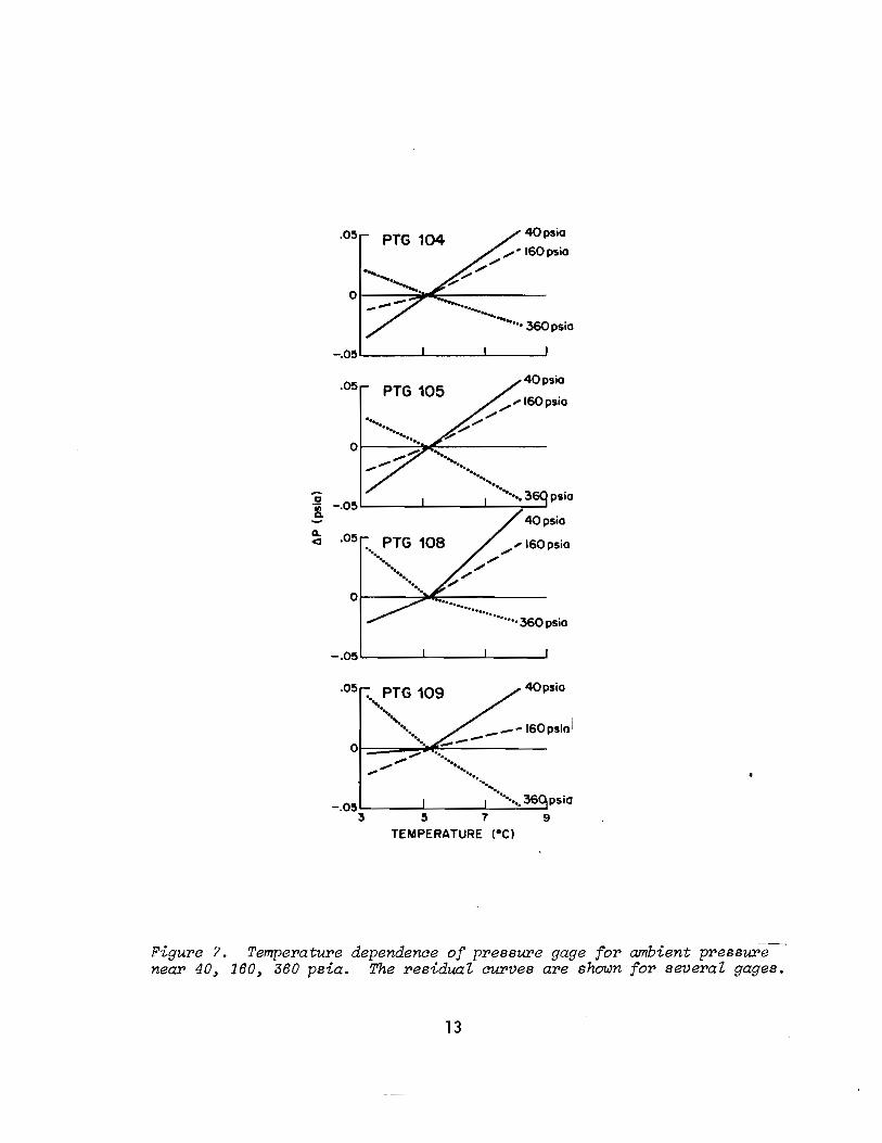
The temperature dependence of the pressure calibration is shown in Fig­ure 7, where the error introduced by using the SoC calibration curve on dataat 3°C and at BOC is plotted. The magnitude of the error depends on pres­sure and is presented for 40, 160, and 360 psia.

A linear temperature dependence is included in the processing of thegages. An average frequency, fa' is calculated for the deployment. Let

10

.050

.030

-.010

-.030

-.050 SECOND ORDER

.050

.030

-.030

-.050 THIRD ORDER

-.070o=---L..---''---=6o=-.........--&---:1-:!:2o::--....L---L----:'180=----'--~2::-:4~0=----"'--......L--:30=-=0:--'-...&--::3...L60- ..........--'--4--120

PRESSURE (psio)

FiguPe 5. Residuals between applied and calculated pressure using asecond- and third-order polynomial in frequency.

11

N

.02

5.

i,iii

iii

iii

Iii

Iii'

,•

I

.02

0

.01

5

o ·iii

0.

(J)

J ~ :::l

o en-

00

5w

·Q

:

-.0

10

-.0

15

-.0

20

-.0

25

1!

!!

!•

!!

!!

!!

!!

•!

!I

!I

,I

o6

012

018

02

40

30

03

60

42

0

PR

ES

SU

RE

(psia

)

Fig

ure

6.

Typ

ical

resi

du

als

betw

een

ap

pli

edan

dca

lcu

late

dp

ress

ure

usi

ng

ath

ird

-ord

erpo

lyno

mia

lin

freq

uenc

y.

40psia

",' 160psio

';.',,,,"PTG 104

0t--~:::iiiJ""::-------

.05

-.05'-------"----'-----J

40psia

",160psiO",

,,/."

PTG 105

psio'--__---' ---L_----,::--.....

Ol---......;.l~,------..........············360 psio

.05

0

-0-.05"&

Cl. .05<I

-.05 '-------'----'------'

40psio'. PTG 109.......

.......'.'.

Ol-==_~··~~-----,. ............

.05

-.05 ........---'-------'---''--.......3 5 7

TEMPERATURE (Oel

Figure 7. Temperature dependence of pressure gage for ambient pressurenear 40, 160, 360 psia. The residual curves are shown for several gages.

13

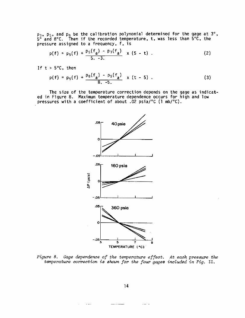
P3, Ps, and Pa be the calibration polynomial determined for the gage at 3°,5° and 8°C. Then if the recorded temperature, t, was less than 5°C, thepressure assigned to a frequency, f, is

p(f) = Ps(f) + Ps(fa) - P3(fa) x (5 - t) (2)5. -3.

If t > 5°C, then

p(f) = Ps(f) + Pa(fa) - Ps(fa) x (t - 5) .8. -5.

(3)

The size of the temperature correction depends on the gage as indicat­ed in Figure 8. Maximum temperature dependence occurs for high and lowpressures with a coefficient of about .02 psiajOC (1 mbjOC) .

•O!l 40psio

ot------::~-----

-.05 .....1-__....1-__....1

160psio

o'iiia.

Q.

<1

360 psio

01------""""--==------

-.05 '-----------JL-__L-~_J

3 5 7 9

TEMPERATURE (·e)

Figure 8. Gage depe'Y'.dence of the temperature effect. At each pressure thetemperature co!'!'ection is shown for the four gages included in Fig. U.

14

3.2 Temperature Calibration

The temperature calibration consists of calibrating the thermistors togive resistance as a function of temperature and calibrating the tempera­ture card (VFSR) to give output counts (frequency) as a function of resist­ance.

The thermistor calibration is performed at NWRCC. Calibration is atseven temperatures from O°C to 30°C in SoC increments. During most of thecalibration period, the thermistors are powered (3.9 V d.c.) to simulatenormal operating conditions with the accompanying self heating.

To measure the resistance, each thermistor is switched to a measuringbridge and the resistance is recorded. Temperature and resistance are re­lated by the Steinhart-Hart equation (Steinhart and Hart, 1968),

(4)

(5)

where T = temperature, oK; R = resistance, ohms; and A, B, C = coefficientsdetermined by a least squares fit to calibration data.

The temperature card (VFSR) is calibrated in the laboratory using aVishay ohmic standard. The VFSR card is adjusted to a signal output per­iod of 1820.4 ~s with an input resistance of 74.440 Kn. Measurements arethen made with seven different input resistors, which correspond to nomi­nal thermistor resistances for temperatures from O°C to 30°C in SoC in­crements. These resistances are 94.98, 74.44, 58.75, 46.67, 37.30, 30.00,and 24.27 Kn. The card calibration is then given by a least squares linearregression of the measured period with the input resistance,, .

R = ao + al ,T

where R is resistance, ohm; T is period, seconds; and ao , al are the re­gression coefficients.

3.3 Pr~ssure Calibration Tests

In addition to the standard calibration" procedures discussed in sec­tion 3.2, several of the ga~es have been subjected to special tests in or­der to study the effect of (a) long-term drift, (b) hysteresis, (c) flowpast the sensor. In this section these tests are discussed and the resultspresented. Although in some cases the results were inconclusive, the prob­lems observed may be of use to other investigators.

3.3.1 Long-term Drift

The drift rate of the Paroscientific transducer specified by the man­ufacturer is less than .01% of full scale per year. For the 400-psiatransducer which we use, this translates into about 3 mb per year. Thedrift rate was established on the basis of repeated comparison between the

15

transducer and a standard. Unfortunately, our newly developed gages wereimmediately deployed in a field experiment, without time for detailed in­tercomparisons of long-term effects. To study these problems we relied onpre- and post-deployment calibrations and on the structure of the fielddata itself. Early results indicated that the gages were stable in termsof relative pressure fluctuations. That is, the derivative of the cali­bration curve, dP/df, at a given pressure, was constant with time. Forthe two gages PTG-100 and PTG-102, which were calibrated in March 1976and February 1977, the change in Ap/Af was .01%. This small drift will notsignificantly affect the pressure determination.

To check for a slow drift in the absolute pressure measurement, pre­and post-deployment calibrations were considered. These did not yield aconsistent pattern for any gage. There are several possible reasons fordiscrepancies between calibrations: the gage height relative to the pres­sure source, the clock frequency drift, pressure transducer hysteresis,pressure transducer drift. To investigate the validity of the absolutepressure determinations, we calibrated a gage, completely disconnected thegage from the pressure tester, reconnected it, and calibrated the gageagain. The results shown in Figure 9 indicate that differences of order.025 psia (about 1.5 mb) occurred between the two tests. These differ­ences are comparable to the pre- and post-deployment differences. Thecause of the discrepancy has not been found, although pressure transducerhysteresis will contribute. At present we rely on the long-term trend ob­served in the data to set an upper limit on the transducer drift. Thisdata is discussed in section 5.1.

3.3.2 Pressure Transducer Hysteresis.

Pressure gage hysteresis has been measured for several units. Thecalibration was first performed from 40 psia to 360 psia and then from 360psia to 40 psia. Pressure to the gage was maintained while the weightswere being changed. ' Results in Figure 10 show maximum hysteresis of about.06 psia (4 mb). Since the gage is subjected to nearly constant pressure(~ 3 psia) when it is deployed, the hysteresis is not considered important.

3.3.3 Bernoulli Effect

A decrease in pressure may result from flow around the sensor port.This Qynamic pressure effect varies as

AP = ~plvl2 (6)A rough calculation predicts a pressure change of 5 mb for a 100 cm/s cur­rent. However, the geometry of the pressure port is important and the ef­fect could vary significantly with instrument orientation. To check theimportance of the Bernoulli effect, we towed a PTG in the U.S. Army Corpsof Engineers Bonneville Test Facility. The instrument was vertical andtowed horizontally (i.e. pressure port was perpendicular to flow) atspeeds of 20 cm/s and 100 cm/s. At the low speed the pressure response was

16

42

0

,,0

....

...,

...p

----

<)'

""0

~~

~

~PTG-108

cI~

~~

~~

cI~

~

~~

~

•/PT

G-l04

--./

'---

/0

-.0

16

-.0

12

.02

0

-.0

20

.012

.00

8

·02

41

II

II

II

II

II

II

I'~J

II

II

I

.016

~0

<[ ::> 9

-.0

04

(/) w 0::c .~

.00

4

--'

""oJ

Fig

ure

9.R

esid

ua

lsbe

twee

na

pp

lied

pre

ssu

rean

da

ala

ula

ted

pre

ssu

re.

The

aa

lau

late

dp

ress

ure

isba

sed

onth

ea

ali

bra

tio

nau

rve

foun

ddu

ring

the

firs

tem

ersi

on(s

eete

xt)

.

-

.07

01

',

,,

,•

,,iii

,,

,,Ii'

,i

I

.05

0

PT

G-1

00

-'" 00

,~.0

30

lit a. VI

.J-

01

0<l

:•

::> 9 VI

W Q:

-.0

30

-.0

50

1

..,07

01.

.,,

.,.

....

....

..,

,...-",.!

1iii

iI

o6

012

01

80

24

03

00

36

04

20

PR

ES

SU

RE

(ps

io)

Fig

ure

10.

Pr~ssure

gage

hys

tere

sis.

The

calc

ula

ted

pre

ssu

reis

base

don

the

cali

bra

tio

ncu

rve

fit

toth

ed

ata

whe

nth

ep

ress

ure

Was

incr

easi

ng

.Th

ere

sid

ual

ssh

own

are

betw

een

calc

ula

ted

and

mea

sure

dp

ress

ure

for

pre

ssu

res

decr

easi

ng.

negligible (i.e., < 0.5 mb). At 100 cm/s the pressure measurements werenoisy; however, an average change of 5 mb was observed.

The importance of this effect will depend upon the application of thePTG. For bottom measurements in the Gulf of Alaska the effect is not con­sidered important. Velocities 10 m from the bottom are generally less than30 cm/s. The velocity 1 m above the bottom (the approximate height of thepressure port) will be less than this. In tidal channels, large flows maybe observed and the effect might be important.

4. DATA PROCESSING

4.1 Processing of Data Taken at Sea

The gage writes a three-word record (clock, pressure, temperature)every 900 s onto a four-track cassette tape. The cassette records aretransferred to seven-track (computer-compatible) tape with a Sea Data model12 reader and a Digi-Data Corporation recorder. During this process, thelogical structure of the data and the parity are checked. Figure 11 is aflow chart describing the data processing system.

Program TG-1 buffers in seven-track tape record and unpack the bitsinto clock, pressure, and temperature words. If an error is encountered,its type is indicated by a coded error word. Temperature and pressurewords are converted to frequency (i.e., divided by the sample interval of900 s). Temperature and/or pressure calibration polynomials may be ap­plied if they are available. Program output is on seven-track tape andeither microfiche or line printer list. Each output record consists of:

(1) error word(2) c1oc k word(3) pressure frequency(4) temperature frequency(5) pressure (db) (if calibration coefficients used)(6) temperature (OC) (if calibration coefficients used)(7) 1ine count.

The clock word is checked (the clock should increment every 450 s),and records with an improper clock word are visually flagged on the outputlisting. The output also includes the total number of records encountered,with errors and improper clock words.

A GMT time and date is assigned to every record from the following:(1) pre-deployment clock reset time, (2) pre-deployment and/or post-re­covery "events" (i.e., pressure "pump-up" with a hand pump at a known time),and (3) deployment and recovery checkoff sheets.

With this information, basic statistics (mean, standard deviation,variance, skewness, kurtosis, extrema) can be calculated for pressure and

19

DATA PROCESSINGFOR

PRESSURE GAUGES

CALI BRATtONCOEFFICIENTS

TG 1

LISTINGMICROFICHE

TG 2-

LISTINGMICROFICHE

Figure 11. Flow ahart of preSSUl'e proaessing programs.20

temperature (either frequencies or actual values) during the period of de­ployment. (Values with bad error words are omitted from calculations.)If the pressure or temperature seems incorrect, the microfiche listing isvisually scanned or the data is plotted to locate" "bad" points. If theincorrect data are accompanied by error tags, they will be replaced auto­matically by Program TG2. If not, TG2 has options to permit insertion orreplacement of bad values. If many data values are bad, another computerprogram is used to display the bit patterns of the words in question. Ifnecessary, these patterns can be modified by rerunning program TGl withtemporary modifications.

Program TG2 applies time/date words to each record and replaces, bylinear interpolation, any record with an error tag. It has options for ed­iting: (1) inserting data values specified on input, (2) replacing datavalues specified on input, (3) replacing data records which have tempera­ture or pressure values outside specified limits; and for calibration:(1) applying calibration coefficients for temperature and/or pressure,(2) applying a correction for time dependence of the pressure calibration,and (3) applying a correction for temperature dependence.

Output includes the number of values replaced by editing options,the line count of values outside pressure or temperature windows, the cali­bration coefficients, and the last data record. The following output val­ues are written on seven-track tape and are optionally listed on microfiche:

(1) time/date (GMT)(2) pressure (db)(3) temperature (OC)(4) line count.

This magnetic tape is used for most of the subsequent plotting andtime series data analysis performed with standard programs in the PMEL pro­gram library.

4.2 Processing of Calibration Data

Figure 12 is a flow chart of the data processing system for calibra­tion of pressure gages. The cassette tape is translated to a seven-tracktape which is read by program TG1, as described in section 4.1.

Program PRCAL calculates the coefficients of the third-order calibra­tion polynomial by the least squares method. Input to this program con­sists of the seven-track tape generated by program TG1, the calibrationpressures applied at NWRCC, the times when they were applied, and the pres­sure gage clock reset time. PRCAL lists and punches the calibration data(NWRCC-applied pressures and average frequencies). It also plots the resi­duals of the curve fit and lists the least squares coefficients.

5. SAMPLE RESULTSAs examples of pressure measurements obtained with the PTG, records

from four locations in the Northeast Gulf of Alaska are presented. These

21

•

TG t.

CAUS. DATA(FREQ, PRESS.

PAIRS

MICROFICHEOPTIONAL

CALIB. PRESS.6 TIMES

RESET TIME

PRCALCALC. CALIa.

COEFF.

LIST OUTCALIB. COEFF.OR AVG. p,T

CALCOMPPLOTS OF

CALIB.RESIDUALS

Figure 12. Flow chart of pressu:t'e calibration processing programs.

22

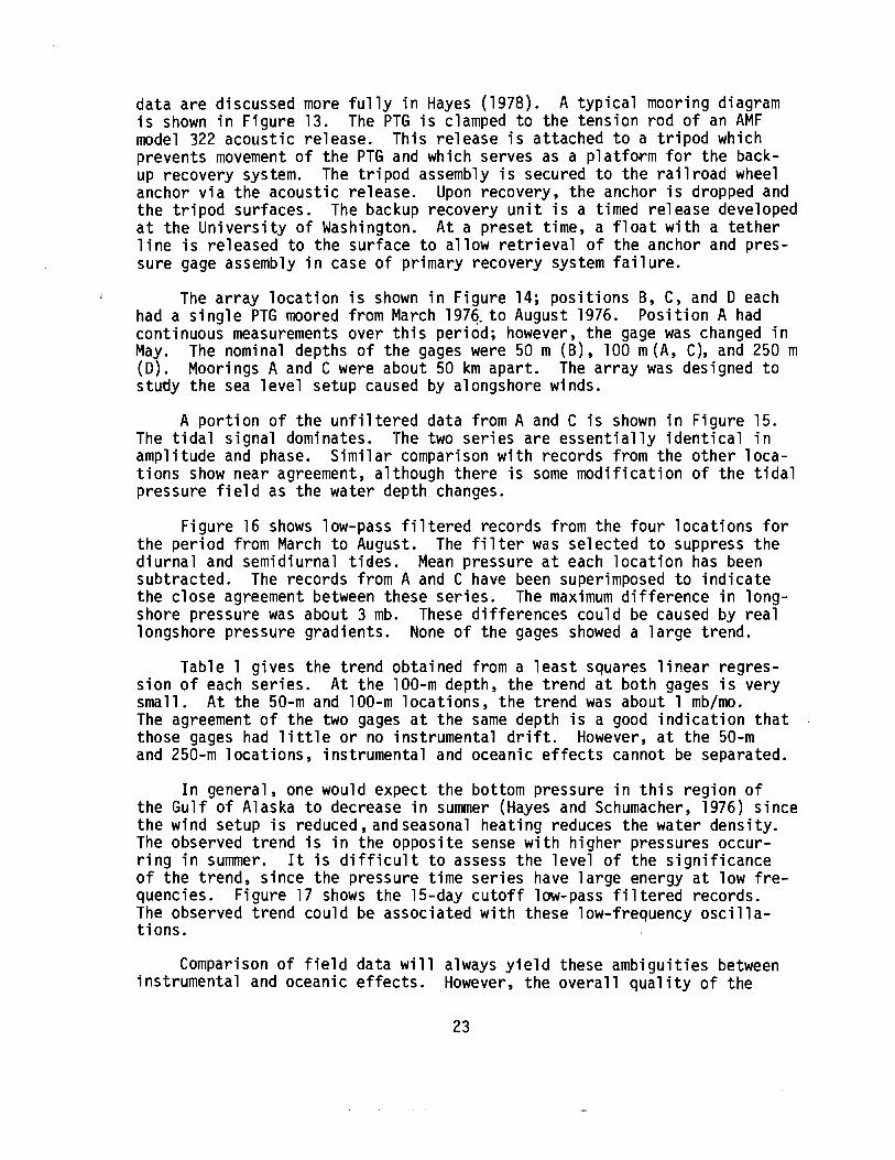
data are discussed more fully in Hayes (1978). A typical mooring diagramis shown in Figure 13. The PTG is clamped to the tension rod of an AMFmodel 322 acoustic release. This release is attached to a tripod whichprevents movement of the PTG and which serves as a platform for the back­up recovery system. The tripod assembly is secured to the railroad wheelanchor via the acoustic release. Upon recovery. the anchor is dropped andthe tripod surfaces. The backup recovery unit is a timed release developedat the University of Washington. At a preset time. a float with a tetherline is released to the surface to allow retrieval of the anchor and pres­sure gage assembly in case of primary recovery system failure.

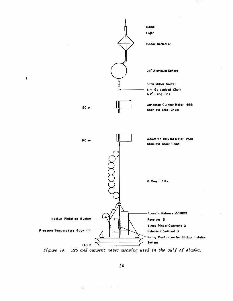
The array location is shown in Figure 14; positions B. C. and D eachhad a single PTG moored from March 197q. to August 1976. Position A hadcontinuous measurements over this period; however. the gage was changed inMay. The nominal depths of the gages were 50 m (B). 100 m(A. C). and 250 m(D). Moorings A and C were about 50 km apart. The array was designed tostudy the sea level setup caused by alongshore winds.

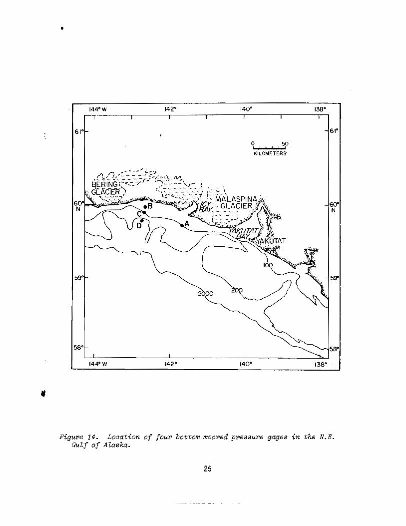
A portion of the unfiltered data from A and C is shown in Figure 15.The tidal signal dominates. The two series are essentially identical inamplitude and phase. Similar comparison with records from the other loca­tions show near agreement. although there is some modification of the tidalpressure field as the water depth changes.

Figure 16 shows low-pass filtered records from the four locations forthe period from March to August. The filter was selected to suppress thediurnal and semidiurnal tides. Mean pressure at each location has beensubtracted. The records from A and C have been superimposed to indicatethe close agreement between these series. The maximum difference in long­shore pressure was about 3 mb. These differences could be caused by reallongshore pressure gradients. None of the gages showed a large trend.

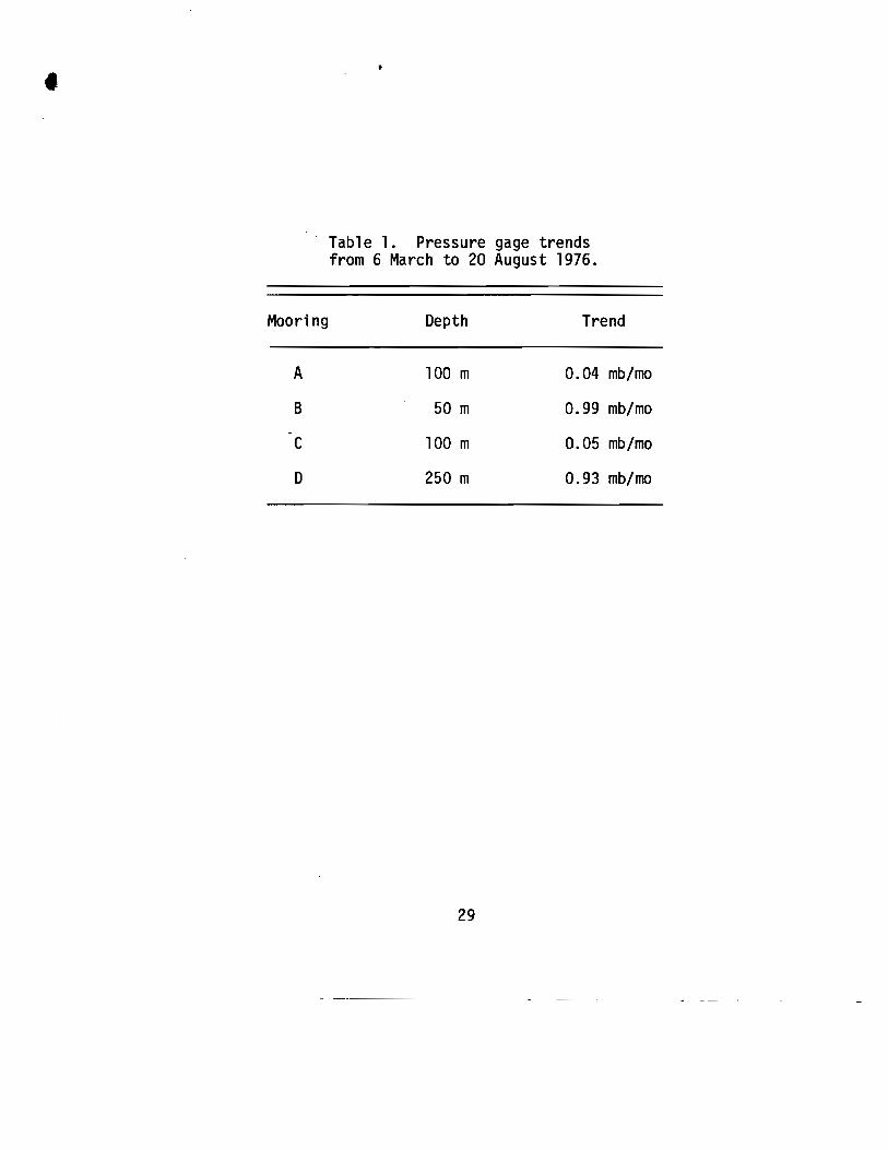
Table 1 gives the trend obtained from a least squares linear regres­sion of each series. At the 100-m depth. the trend at both gages is verysmall. At the 50-m and 100-m locations. the trend was about 1 mb/mo.The agreement of the two gages at the same depth is a good indication thatthose gages had little or no instrumental drift. However. at the 50-mand 250-m locations. instrumental and oceanic effects cannot be separated.

In general. one would expect the bottom pressure in this region ofthe Gulf of Alaska to decrease in summer (Hayes and Schumacher. 1976) sincethe wind setup is reduced. and seasonal heating reduces the water density.The observed trend is in the opposite sense with higher pressures occur­ring in summer. It is difficult to assess the level of the significanceof the trend, since the pressure time series have large energy at low fre­quencies. Figure 17 shows the 15-day cutoff low-pass filtered records.The observed trend could be associated with these low-frequency oscilla­tions.

Comparison of field data will always yield these ambiguities betweeninstrumental and oceanic effects. However, the overall quality of the

23

Radio

50 m DO

Radar Reflector

28" Aluminum Sphere

3 ton Miller Swivel

3 m Galvanized Chain1/2" Lono Link

Aanderaa Current Met.r 1833

Stainless St••1Chain

90 m [10 Aanderaa Current Met.r 2501

Stainles. Steel Chain

Firing Mechanism for Backup Flotation

System

Timed Pinoer Command 2

Release Command 3

Receiver 8

8 Viny Floats

I-----Acoustic Release 601829

110m

PTG and auI'roent metero mooroing used in the Gulf of Alaska.

Backup Flotat ion System----r

Figure 13.

Pressure Tempera tur. Gaoe 102 ---t---t--;........J.1~-=~

24

•

o 50, , t , , ,

KILOMETERS

Figure 14. Location of four bottom mooped ppessure gages in the N.E.Gulf of Alaska.

25

MOORING C

•

US,....-----------------~-------,

MOORING A

uo

--II)...8·0 lOS .J----r----r---.,...--'"'T"""--_r_--_r_---r---__--.,...---+CD'0....UJ

S 105......----------------------------.enf30:::4.

100

851+0---t"Tl--......,.12--~13:---"""":""t4:---"""""':'!tS::--"""7!18::--"""7!17;--"""7!t8;--~18::----:±20tilt?I

Figure 15. A porotion of the unfiZteroed proessure roeaom at mooroings A and C(100 m nominaZ depth).

26

:.--------------------~------0.15

0.t5 --------------------------------,

III..o.0UQ)'C

wcr::>V>V>Wcr0..

MOORING A,e (100m)

0.15 ------------------------------,

MOORING 0 (250m)

-0 .t5 -bmTTT"""mTTTrrrrlllmnTl'TTl"mTTTnrmnTTlTnjt'I'TTTTmm'I'TTTTmmTmT'":trmrTTTTTTTllTlTTTTTmmnltfnmmmrTTTTTmmrl'lTlT+""""rrmn..l-

JR APR I1RY JUN JUL FlUO76 76 76 76 75 76

Figu:r>e 16. Low pass fiZte:r>ed data at the four' locations. The mean of eachp:r>e88ur'e was :r>emoved. FiZte:r> cutoff is about 3 days.

27

0.15~---------------------------'T

0.00

MOORING B (50 m)

O.lS ........---;...-.------------------------T

-fcD.~

'0-

MOORING Ate (100m)

0.15-----------------------------....

0.00

MOORING 0 (250 m)

-G.151-""'"""'"-rr+--"""''''''''~.......,''''''''"''''"'''mnf'"'''mm'"'""""mnf"""mm'''"''mm-~rmm''''"''rd-8 1 1 1 1 1tIIR fI'I tIAY .... .u. II»'18 '18 '18 '18 '18 78

Figupe 1? Low pass fi Ztel'ed data at the foUl' loaations. Fi Ztel' autoff is15 days.

28

•

Table 1. Pressure gage trendsfrom 6 March to 20 August 1976.

Mooring

A

B

C

D

Depth

100 m

50 m

100 m

250 m

29

------

Trend

0.04 mb/mo

0.99 mb/mo

0.05 mb/mo

0.93 mb/mo

pressure series and the small trends observed compared to the signals ofinterest ( 2- to 10-day storm events) are encouraging. The PTG has proveda valuable research tool for studying ocean dynamics over continentalshelves. As additional data is accumulated, we expect to see the use of ~the gage extended, and new information on instrumental characteristicswill be available. •

AckncwZedgements. We wish to acknowledge the encouragement which D.Halpern gave in the development of this gage. Much of the early designwork and prototype development was done by A. M. Zwilling.

The development was supported in part by the Bureau of Land Managementthrough interagency agreement with the National Oceanic and Atmospheric Ad­ministration, under which a multi-year program responding to needs of petro­leum development of the Alaskan Continental Shelf is managed by the OuterContinental Shelf Environmental Assessment Program (OCSEAP) Office.

30

6. REFERENCES

Culverhouse, B. (1977): Self-contained digital tide measurement system.NOAA Tech. Memo. ERL AOML-24.

Hayes, S. P. (1978) Variability of current and bottom pressure acrossthe continental shelf in the northeast Gulf of Alaska. ~. Phys.Oceanogr. (in press).

Hayes, S. P. and J. D. Schumacher (1976): Description of wind, current,and bottom pressure variations on the continental shelf in the N.E.Gulf of Alaska from February to May 1975. ~. Geophys. Res., 18:6411-6419.

Paros, J. (1976): Digital pressure transducers. Meas. and Data, 10:74-79.

Steinhart, J. S., and S. R. Hart (1968): Calibration curves for thermis­tors. Deep-Sea Res., 15:497-503.

31