NOAA Holistic Climate and Earth System Model Strategy Phase I

1

NOAA Technical Report OAR CPO-3

NOAA Holistic Climateand Earth SystemModel StrategyPhase I: Current Statedoi:10.7289/V5Z31WKK

NOAA Technical Report OAR CPO-3NOAA Holistic Climate and Earth System Model StrategyPhase I: Current Statedoi:10.7289/V5Z31WKKClimate Program OfficeSilver Spring, MarylandMarch 2015

Report Team AuthorsDavid G. DeWitt1, Stanley G. Benjamin2, Brian D. Gross3, R. Wayne Higgins4, Monika Kopacz4, Arun Kumar1, Annarita Mariotti4 , Suranjana Saha5, Hendrik L. Tolman5

Affiliations1Climate Prediction Center, NOAA/NWS/NCEP, College Park, Maryland2NOAA/Earth System Research Laboratory, Boulder, Colorado3NOAA/Geophysical Fluid Dynamics Laboratory, Princeton, New Jersey4Climate Program Office, NOAA/OAR, Silver Spring, Maryland5Environmental Modeling Center, NOAA/NWS/NCEP, College Park, Maryland

United StatesDepartment of CommercePenny PritzkerSecretary

National Oceanic andAtmospheric AdministrationDr. Kathryn D. SullivanUndersecretary for Oceans andAtmospheres

Office of Oceanic andAtmospheric ResearchCraig McLeanAssistant Administrator

Notice from NOAAMention of a commercial company or product does not constitute an endorsement by NOAA/OAR. Use of information from this

publication concerning proprietary products or the tests of such products for publicity or advertising purposes is not authorized.

Any opinions, findings, and conclusions or recommendations expressed in this material are those of the authors and do not

necessarily reflect the views of the National Oceanic and Atmospheric Administration.

NOAA Holistic Climate and Earth System Model StrategyPhase I: Current State

3

AbstractThis report describes Phase I of a two-phase study proposed and organized by the NOAA Climate Program Office (CPO) in early 2014 for the development of a NOAA Holistic Climate and Earth System Modeling Strategy. Defining NOAA’s strategy for global climate and earth system modeling for research and operations allows NOAA’s investments in this area to be optimally targeted and leveraged, facilitates linkages with broader environmental modeling efforts within NOAA and outside of NOAA, and enhances NOAA’s participation in the interagency Earth System Prediction Capability initiative. A strategy also helps to identify gaps and opportunities to advance NOAA’s global climate and earth system models and identify resources and synergies needed to maximize the return on those investments. In addition, the 2012 National Research Council report on “A National Strategy for Advancing Climate Modeling” prompts a careful reconsideration of NOAA’s strategy in this area.

Phase I defines the current state of, and plans for, NOAA’s global climate and earth system models, developed at the Geophysical Fluid Dynamics Laboratory, the Earth System Research Laboratory, and the National Centers for Environmental Prediction Environmental Modeling Center. This report lays the necessary groundwork for the planned second phase of the CPO proposed study whose ultimate goal is to present potential future model development pathways contributing to the definition of a holistic strategy to advance NOAA global climate and earth system models for research and operations.

1. IntroductionThe National Oceanic and Atmospheric Administration (NOAA) climate and earth system modeling (NESM) enterprise is an essential science and technology capability for the successful execution of the NOAA Next-Generation Strategic Plan (NGSP). The development of these models occurs at the Geophysical Fluid Dynamics Laboratory (GFDL),

the Earth System Research Laboratory (ESRL), and the National Centers for Environmental Prediction (NCEP) Environmental Modeling Center (EMC). Key societally relevant outputs supported by these models include experimental and operational intraseasonal to interannual (ISI) climate predictions; decadal to centennial climate projections and attribution studies; experimental predictions and projections of biogeochemical processes on timescales from weeks to centuries; climate reanalysis and monitoring; and enhanced understanding of the earth system and its future evolution. The portfolio of model research and development work includes both lower-risk, incremental applied research and higher-risk, higher-reward exploratory research. This breadth of research and development supports improvements to the current operational systems and simultaneous exploration of promising areas for future model improvements, and is required in order to meet the current and future needs of NOAA stakeholders.

Vigorous and productive collaboration has occurred between the different centers of the NESM enterprise for several decades. An area of especially active collaboration is the development and application of climate models to the ISI forecast problem. In this area, collaboration has included both cross-center exchange of component models and development of multi-model ensemble (MME) forecast systems. In the former case, EMC has used various versions of the GFDL Modular Ocean Model (MOM) as the ocean component in its ISI forecast system since the mid-1990’s, while in the latter, both GFDL and EMC produce ISI forecasts for the North American Multi-Model Ensemble (NMME; Kirtman et al., 2014). MME forecasts typically have higher accuracy and increased reliability compared to the best individual model ensemble forecast system (Peng et al., 2002), and can be a cost-effective way to leverage existing activities at the different NOAA modeling centers. However, it should also be recognized that the MME approach does not replace the fundamental need for continual improvement of the individual models used

3

4

to construct the MME. The NMME is also an excellent example of the NESM enterprise working together with the research community to produce products that contribute to both research and operational modeling goals. In addition to the collaborative activities, each of the modeling centers makes unique contributions to NOAA’s mission. EMC produces the operational NOAA numerical guidance for timescales from hours to seasons, while GFDL produces the NOAA long-term climate projections that are used in the Coupled Model Intercomparison Project (CMIP) and the Intergovernmental Panel on Climate Change (IPCC) processes. GFDL also leads the NOAA earth system modeling effort and serves as the agency lead for evaluating the potential of decadal predictions. Previously, ESRL has focused on the short- to medium-range weather forecasting problem, but is now developing a coupled ocean-atmosphere model that will be applied to the ISI timescale.

This report presents a snapshot of the current NESM models used at GFDL, EMC, and ESRL. For the purposes of this report, climate and earth system models are defined as follows: Climate models simulate the physical system, and historically have included atmosphere, land, ocean, and sea-ice component models. Earth system models build on climate models by adding a global carbon cycle, and typically include prognostic models for atmospheric chemistry, terrestrial ecosystems, and ocean biogeochemistry. The focus of this report is on global coupled models used for research and operations for the subseasonal to centennial timescale. However, it is important to recognize that weather and climate processes interact and influence each other. Therefore, within NOAA, development of climate and weather models is done in a holistic way to ensure fidelity in simulation of the continuum of weather and climate variability. This report serves as a high-level single source of information that can inform scientists

interested in utilizing these models, and NOAA managers interested in learning about the current state of the NESM portfolio. It should be emphasized that by design this is a brief report, and, hence, can only present a sampling of the rich work being done within the NESM enterprise in support of the NGSP. The reader is encouraged to examine the more extensive documentation of research results and datasets referenced in the text and the appendix.

Section 2 describes the GFDL Coupled Model version 2.1 (CM2.1), version 2.5 (CM2.5), version 3 (CM3), and the Earth System Model version 2M (ESM2M). Section 3 describes the EMC Climate Forecast System version 2 (CFSV2). Section 4 describes the coupled ESRL Flow-following finite-volume Icosahedral Model (FIM) - icosahedral Hybrid Coordinate Ocean Model (iHYCOM). Section 5 presents a brief overview of previous and current NESM collaborative activities. Section 6 describes universal challenges facing the NESM enterprise, and Section 7 presents a brief summary of the report. The Appendix has a table that gives a high-level view of the models covered in the report. It also provides links to more comprehensive documentation available for the models, and the location of model code and data.

2. GFDL Climate and Earth System ModelsGFDL’s mission is to advance scientific understanding of climate and its natural and anthropogenic variations and impacts, and improve NOAA’s predictive capabilities, through the development and use of world-leading computer models of the earth system.

2.1 CM2.1

2.1a Model DescriptionCM2.1 was the first NOAA model used for both experimental seasonal to interannual prediction and centennial-scale climate change projections. Comprehensive documentation of the physical and dynamical formulations of CM2.1 is given in Anderson


5 5

et al. (2004), Delworth et al. (2006), and Gnanadesikan et al. (2006). The resolution of the atmospheric (AM2) and land (LM2) component models is 2° latitude by 2.5° longitude. The atmospheric model has 24 vertical layers with a top at 3.65 hPa. The shortwave radiation scheme follows Freidenreich and Ramaswamy (1999) and includes absorption by H2O, CO2, O3, and O2; molecular scattering; and absorption and scattering by aerosols and clouds. The longwave radiation scheme is that of Schwarzkopf and Ramaswamy (1999). Deep convection is modeled using the relaxed Arakawa-Schubert (RAS) scheme of Moorthi and Suarez (1992). Convective momentum transport is handled with a downgradient diffusion formulation. The cloud microphysics parameterization follows Rotstayn (1997), with an updated treatment of mixed phase clouds (Rotstayn et al., 2000). The cloud fraction is treated as a prognostic variable following Tiedtke (1993). Aerosol indirect effects are not modeled.

The CM2.1 Ocean Model (OM3.1) is based on MOM4 (Griffies et al., 2005) and has horizontal resolution of 1° in latitude and 1° in longitude with progressively increasing meridional resolution equatorward of 30° latitude. In the equatorial region, the meridional resolution is approximately 0.33° in order to resolve the equatorial waveguide and current systems. OM3.1 uses a tripolar grid (Murray, 1996) in order to avoid polar filtering over the Arctic. There are 50 vertical layers with 10 meter spacing in the upper 220 meters, and the bottom depth is 5.5 km. OM3.1 employs an explicit free surface with a freshwater flux boundary condition. Vertical mixing is modeled using the K-Profile Parameterization (KPP) mixed layer scheme of Large et al. (1994). Shortwave radiation absorption follows Morel and Antoine (1994) and includes the mean annual cycle of chlorophyll concentration. The horizontal advection scheme is based on the third-order upwind-biased approach of Hundsdorfer and Trompert (1994), including the Sweby (1994) flux limiters. Isoneutral mixing is handled following Griffies et al. (1998). Mesoscale eddies are parameterized

using the skew-flux approach of Griffies (1998), with a local treatment of the quasi-Stokes streamfunction (Gent and McWilliams, 1990; Gent et al., 1995). Lateral viscosity is treated using an anisotropic scheme in the tropics following Large et al. (2001). In this scheme, the background viscosity is large in the east-west direction, but small in the north-south direction except near the western boundaries. The background viscosity is isotropic in the extratropics.

The CM2.1 Land Model (LM2) is the Land Dynamics Model of Milly and Shmakin (2002), which includes a river routing scheme that transports runoff collected over the model’s drainage basins to river mouths, where it is treated as a freshwater source to the ocean model. The land cover type distribution is a combination of a potential natural vegetation-type distribution and a historical land use distribution dataset. The potential natural vegetation classification has 10 vegetation or land surface types (broadleaf evergreen, broadleaf deciduous, mixed forest, needle-leaf deciduous, needle-leaf evergreen, grassland, desert, tundra, agriculture, and glacial ice).

The sea ice component model is the Sea Ice Simulator (SIS; Winton, 2000). SIS is a dynamical model with two ice and one snow layer, and five ice thickness categories. Ice internal stresses are calculated using the elastic-viscous-plastic technique of Hunke and Duckowicz (1997), while the thermodynamics treatment is a modified Semtner (1976) three-layer scheme.

Coupling between the atmosphere, land, ocean, and ice models occurs every 2 hours in order to resolve the diurnal cycle.

2.1b Model Performance and Sample ApplicationsCM2.1 was one of two GFDL models that contributed to the CMIP version 3 (CMIP3) and the IPCC Assessment Report No. 4 (AR4). Independent comparison of IPCC AR4/CMIP3 models shows that CM2.1 produced one of the better ENSO simulations (van Oldenburgh et

6

al., 2005) and simulated the observed modern-era atmospheric circulation better than many of the other models (Reichler and Kim, 2008). CM2.1 seasonal forecasts are produced in real-time for the NMME project and are provided to the Climate Prediction Center (CPC) for use in generating its operational predictions. The skill of CM2.1 monthly and seasonal forecasts (Kirtman et al., 2014; Becker et al., 2014) is competitive with similar models from other forecast centers. Further, the CM2.1 skill is at least partially complementary to other models from US institutions such as the EMC CFSV2. CM2.1 participated in the CMIP5 experimental decadal hindcasts.

An ensemble coupled data assimilation (ECDA; Zhang et al., 2007) system based on CM2.1 was developed and used to initialize the GFDL CMIP5 decadal forecasts and GFDL’s contributions to the NMME. The ECDA system assimilates oceanic temperature, salinity, and sea surface temperature (SST), while constraining the atmospheric state using NCEP’s analysis. An ECDA-based ocean reanalysis is available for the period 1961 to 2012. A link to the ECDA re-analysis data is provided in the Appendix.

2.2 CM2.5

2.2a Model DescriptionThe CM2.5 atmospheric model dynamics and physics are nearly identical to those for CM2.1. The major difference in the atmospheric models is that the CM2.5 atmospheric model has increased horizontal resolution (50 km) and vertical resolution (32 layers) compared to CM2.1. Complete documentation of CM2.5 is given in Delworth et al. (2012).

Key differences between the ocean component models for CM2.1 and CM2.5 as documented in Delworth et al. (2012) include:

• CM2.5 has horizontal resolution of 0.25°.

• CM2.5 does not use a mesoscale eddy parameterization.

• CM2.5 uses a parameterization for the effects of sub-mesoscale, mixed layer eddies (Fox-Kemper et al., 2011).

• CM2.5 uses the piecewise parabolic method (PPM; Colella and Woodward, 1984; Huynh, 1996), which is a third-order finite volume advection scheme. PPM is more accurate and less dissipative than the advection scheme used in CM2.1.

• CM2.5 does not use explicit lateral diffusion or background vertical diffusion.

• Coastal tidal mixing uses the scheme of Lee et al. (2006).

• Internal tidal mixing uses the scheme of Simmons et al. (2004).

• CM2.5 uses MOM4.1 (Griffies, 2010) with a z* vertical coordinate (Griffies et al., 2011).

• CM2.5 has a very low horizontal viscosity. This is achieved by use of the Smagorinsky (1993) biharmonic formulation (Griffies and Hallberg, 2000) with a prescribed background viscosity that is enhanced next to western boundaries.

• CM2.5 explicitly models the flow between straits, such as the Atlantic and the Mediterranean.

• A version of CM2.5 with higher ocean resolution, denoted CM2.6, was developed. CM2.6 is identical to CM2.5 except that the ocean horizontal resolution is increased to 0.1° . The simulation of ocean eddy activity is very realistic in CM2.6 (Delworth et al., 2012). Comparison of CM2.5 and CM2.6 simulations, predictions, and projections contribute to our understanding of the role of ocean eddies in climate variability on different timescales.

New capabilities in the CM2.5 land model, the Land Model version 3 (LM3; Delworth et al., 2012; Milly et al., 2014a; Shevliakova et al., 2009) include:


7

• A multilayer model of snowpack above the soil.

• A continuous vertical representation of soil water that spans both the unsaturated and saturated zones.

• A frozen soil-water phase.

• A parameterization of water table height, saturated-area fraction, and groundwater discharge to streams derived from standard groundwater-hydraulic assumptions and surface topographic information.

• Finite velocity horizontal transport of runoff via rivers to the ocean.

• Lakes, lake ice, and lake-ice snow packs that exchange mass and energy with both the atmosphere and the rivers.

• Consistent, energy-conserving accounting of the sensible heat content of water in all of its phases.

• The carbon balance and determination of vegetation structure, phenology, and function follow Shevliakova et al. (2009).

Inclusion of these new capabilities in LM3 improves the representation of the physical system.

2.2b Model Performance and Sample ApplicationsKey improvements in the simulated climate compared to CM2.1 include a reduction in the double ITCZ in the tropical Pacific, an improved simulation of ENSO, and improvements to the regional precipitation features, including the Indian monsoon and Amazonian rainfall (Delworth et al., 2012). Kapnick and Delworth (2013) found significant improvements in the simulated CM2.5 snowfall magnitude and distribution compared to CM2.1. Knutti et al. (2013) showed that CM2.5 simulations of surface temperature and precipitation were among the best for CMIP5-class models, in terms of agreement with present day climate. Further information on performance and applications of CM2.5 are found in Delworth (2014), Kapnick (2014), Vecchi (2014a), and Wittenberg (2014).

2.3 CM2.5-Forecast-Oriented Low Ocean Resolution (FLOR)

2.3a Model DescriptionThe CM2.5-FLOR model is identical to CM2.5 except that it uses the lower-resolution CM2.1 Ocean Model (OM3.1). FLOR is computationally less expensive than CM2.5, and is used for climate forecasting on the intraseasonal to interannual timescale. Currently, it is being used for experimental seasonal hurricane forecasts, and forecasts of the statistics of extreme weather. The lower computational cost compared to CM2.5 enables the use of larger ensembles, which can help to identify the signal for phenomena such as extreme events that have a small signal-to-noise ratio. The larger ensembles will also allow better definition of the model probability distribution function and quantification of uncertainty.

2.3b Model Performance and Sample ApplicationsA number of studies have compared the simulation and forecast characteristics of FLOR with other versions of the GFDL coupled model. Extended simulations with FLOR show improved ENSO teleconnections, and reduced biases of surface temperature and precipitation compared to CM2.1 (Jia et al., 2015). Forecast skill of tropical Pacific SST associated with ENSO is improved for FLOR over CM2.1. ENSO teleconnections, and surface temperature and precipitation biases are very similar for FLOR and CM2.5 (Jia et al., 2015). In a groundbreaking study, Vecchi et al. (2014b) showed that FLOR produces skillful seasonal forecasts of the spatial distribution of tropical cyclone activity. Msadek et al. (2014) found that FLOR produces skillful forecasts of Northern Hemisphere summer sea ice extent out to 6 months lead. This level of skill was similar to that found for CM2.1. However, the FLOR forecasts were shown to have improved fidelity in simulating the climatological atmospheric circulation and sea ice mean state in the Arctic compared to CM2.1. FLOR seasonal forecasts are produced in real-time for the NMME

8

project and are provided to CPC for use in generating its operational predictions. Further information on performance and applications of FLOR are found in Vecchi (2014a), and Wittenberg (2014).

2.4 CM3

2.4a Model DescriptionCM3 was designed to address emerging issues in climate change, including aerosol-cloud interactions, chemistry-climate interactions, and coupling between the stratosphere and troposphere (Donner et al., 2011). The major changes from CM2.1 occurred in the atmospheric and land component models. The atmospheric component model evolved from AM2 to AM3 (Donner et al., 2011), while the land model evolved from LM2 to LM3 (Milly et al., 2014a; Shevliakova et al., 2009).

Major developments in the atmospheric and land component models compared to CM2.1 include:

• New deep cumulus convection scheme (Donner, 1993; Donner et al., 2001; Wilcox and Donner, 2007).

• New shallow cumulus convection scheme (Bretherton et al., 2004; modified as in Zhao et al., 2009).

• Increased vertical resolution from 24 to 48 layers and raising of model top from 35 to 86 km. The additional vertical layers are added in the upper troposphere and stratosphere. The increased resolution in the stratosphere allows a more comprehensive treatment of stratospheric processes.

• Cloud droplet activation by aerosols (aerosol indirect effect; Ming et al., 2006).

• Subgrid variability of stratiform vertical velocities for droplet activation (Ghan et al., 1997).

• Atmospheric chemistry and aerosols driven

by emissions with advective, convective, and turbulent transport. AM3 calculates the mass distribution and optical properties of aerosols based on their emission, chemical production, transport, and dry and wet removal (Donner et al., 2011; Naik et al., 2013).

• Implementation of a cubed-sphere finite-volume dynamical core that enhances the models parallel computing efficiency (Putman and Lin, 2007).

• New land model, Land Model 3 (LM3; Donner et al., 2011; Milly et al., 2014a; Shevliakova et al., 2009), for land water, energy, and carbon balance. LM3 improves the physical representations of the flow of heat and water through the land, and also includes a dynamic vegetation component. (See CM2.5 for enhanced features over the CM2.1 land model).

• Simulation of atmospheric concentration of 97 chemical species over the full depth of the atmosphere (Naik et al., 2013).

• Tropospheric chemistry is modeled using a modified version of the Model for Ozone and Related Tracers version 2 (MOZART-2; Horowitz et al., 2003; Horowitz et al., 2007).

• Stratospheric chemistry is modeled using the Atmospheric Model with Transport and Chemistry (AMTRAC; Austin and Wilson, 2010).

2.4b Model Performance and Sample Applications Several key differences exist between CM2.1 and CM3 climate simulations and projections. These include:

• The CM3 atmospheric component model (AM3) does a more realistic job simulating aerosol optical depths, scattering properties, and surface clear-sky downward shortwave radiation than the atmospheric component model (AM2) in CM2.1 (Donner et al., 2011).

• CM3 simulates Arctic sea ice with more fidelity and smaller biases than CM2.1. (Griffies et al., 2011).


9

• CM3 has a reduced dry bias over South America and reduced biases in surface clear-sky shortwave radiation (Donner et al., 2011).

• CM3 has a larger warm bias in the interior ocean (Griffies et al., 2011).

John et al. (2012) used CM3 simulations to evaluate the relative role of climate and emissions in determining methane lifetime against loss by the tropospheric hydroxyl radical. Austin et al. (2013) evaluated the ability of CM3 to simulate the variability of stratospheric ozone and temperature from 1860 to 2005. Experiments with CM3 showed that both local and remote aerosols are important for explaining the late twentieth century drying of the South Asian monsoon (Bollasina et al., 2014). Simulations with CM3 conducted by Bollasina et al. (2013) showed that the late twentieth century increase in anthropogenic aerosols contributes to an earlier onset of the Indian monsoon. CM3 was the workhorse GFDL climate model contribution to the CMIP5 and IPCC AR5. Additional applications of CM3 can be found on GFDL’s Climate Change web page (http://www.gfdl.noaa.gov/climate-change).

2.5 Earth System Model version 2 MOM (ESM2M)

2.5a Model DescriptionGFDL developed earth system models including the ESM2M (Dunne et al., 2012a; Dunne et al., 2013) to advance our understanding of how the Earth’s biogeochemical cycles, including human actions, interact with the climate system. ESM2M builds on the CM2.1 climate model. The atmospheric component model of ESM2M has only a few minor code updates from CM2.1.

The ESM2M ocean model differs from that in CM2.1 as follows:

• ESM2M uses a rescaled geopotential vertical coordinate (z*; Stacey et al., 1995; Adcroft and Campin, 2004).

• ESM2M employs the conservative, minimally diffusive, monotonic, multidimensional piecewise parabolic method (MDPP; Marshall et al., 1997).

• The quasi-Stokes streamfunction in the mesoscale eddy parameterization is computed as a boundary value problem over the full column (Ferrari et al., 2010).

• An updated version of the KPP vertical mixing scheme is used (Danabasoglu et al., 2006).

• ESM2M uses an isotropic Laplacian friction combined with western boundary enhanced biharmonic friction.

In ESM2M, atmospheric CO2 is treated as a prognostic tracer that is exchanged between the land, ocean, and atmosphere. The ESM2M land component model is LM3 (see description in section describing CM2.5). Treatment of ocean ecology and biogeochemistry is modeled using the Tracers of Ocean Phytoplankton with Allometric Zooplankton version 2.0 (TOPAZ2). TOPAZ2 uses 30 tracers to model the cycles of carbon, nitrogen, phosphorous, silicon, iron, oxygen, alkalinity, surface sediment calcite, and lithogenic material (Dunne et al., 2012b). Three explicit phytoplankton groups (small, large, and diazotrophic) are modeled using modified growth physiology following Geider et al. (1997).

In an alternative version of ESM2M, ESM2G, an independently developed isopycnal model using the Generalized Ocean Layer Dynamics (GOLD) code base was used. Comparison between these two models allows us to assess the sensitivity of the coupled climate-carbon system to our assumptions about ocean formulation (Winton et al., 2013).

10

2.5b Model Performance and Sample ApplicationsESM2M simulates the present-day climate with similar fidelity to CM2.1 (Dunne et al., 2012a). Polovina et al. (2011) used the ESM2M to define large oceanic biomes in the North Pacific Ocean and to describe their changes over the 21st century in response to IPCC AR4 Scenario A2. Experiments with ESM2M demonstrated that the dominant modes of biological and physical variability may change as the earth system is perturbed under greenhouse gas forcing (Rykaczewski and Dunne, 2010). That result demonstrates the limitations associated with use of historical empirical models to predict future changes. The response of primary production in the Arctic Ocean to future climate change was examined for ESMS2M/ESM2G and 9 other earth system models (Vancoppenolle et al., 2013). The causes and implications of persistent atmospheric carbon dioxide biases were studied in 15 earth system models including ESM2M (Hoffman et al., 2013). GFDL completed all of its integrations for CMIP5 (about 100 in total) with ESM2M and ESM2G. These ESMs have been used to examine the impact of climate change on marine life, ranging from plankton (Stock et al., 2014), to cod (Kristiansen et al., 2014), to endangered leatherback sea turtles (Saba and Stock, 2012). Application of dynamic vegetation in the ESM’s land model has shown that regrowing forests can sequester CO2 and offset the loss of carbon to land-use change (Shevliakova et al., 2009). Additional examples on the use of ESM2M including future plans can be found in Naik (2014), Stock (2014), and Dunne (2014). A broader set of applications using GFDL’s ESMs can be found on GFDL’s Earth System Science web page.

2.6 Future Plans for GFDL Climate and Earth System Modeling (Held, 2014) The next generation GFDL climate model is CM4, which will have a base configuration with a 0.5° atmosphere, and a 0.25° ocean. The goal for CM4 is to have a climate model suitable for projection of climate change up to several hundred years in the future, attribution of climate change over the past century, and prediction on seasonal to decadal timescales. Experience with the previous GFDL

modeling streams is informing development of CM4. The CM4 development process will seek both scientific innovation and incremental bias reduction. Additional information on current plans for CM4 can be found in Adcroft (2014), Golaz (2014), Dunne (2014), Milly (2014b), Shevliakova (2014) and Stock (2014). ESM4 will be based on CM4 and will include a new land model that incorporates comprehensive biogeochemistry (nitrogen, phosphorous, methane, etc.), prognostic aerosols (including dust and biomass burning), sub-grid-scale heterogeneity and a new vegetation succession scheme, enhanced representation of land-use management (fertilizers, water quality, etc.), and the Carbon, Ocean Biogeochemistry and Lower Trophics (COBALT) marine ecosystem model (Stock et al., 2014).

2.7 Software Infrastructure GFDL coupled and earth system models use the Flexible Modeling System (FMS). FMS can utilize the Earth System Modeling Framework (ESMF) wrappers to interchange component models with other centers. An example of this interoperability is the coupling of MOM5 to the EMC Global Forecast System (GFS) as a prototype for the CFSV3. FMS is designed for flexibility, modularity, and extensibility.

3. EMC Climate and Earth System ModelsEMC maintains, enhances and transitions-to-operations numerical forecast systems for weather, ocean, climate, land surface and hydrology, hurricanes, and air quality for the Nation and the global community; for the protection of life and property and the enhancement of the economy.

3.1 CFSV2

3.1a Model DescriptionThe current climate model at EMC is the Climate Forecast System version 2 (CFSV2; Saha et al., 2014). The CFSV2 atmospheric model is the Global Spectral Model (GSM). The GSM has a spectral dynamic core with a triangular truncation of T126, and an associated Gaussian grid with approximately 0.95° resolution.


11

The model is discretized with 64 layers in the vertical and has a model top of 0.3 hPa. Deep convection is treated using the Simplified Arakawa Schubert (SAS; Pan and Wu, 1995; Hong and Pan, 1998). Shallow convection is parameterized following Tiedtke (1993). Vertical diffusion is parameterized following Hong and Pan (1996), with a non-local scheme in the planetary boundary layer (PBL) and a local scheme above the PBL. Land-surface processes are modeled using the four-layer Noah model (Ek et al., 2003). Shortwave radiation is modeled using the Rapid Radiation Transfer Model for General Circulation Models (RRTMG-SW; Iacono et al., 2000; Clough et al., 2005), and longwave radiation is modeled using the RRTMG longwave (RRTM-LW; Mlawer et al., 1997). Interaction between the clouds and radiation is handled by the Monte Carlo independent column approximation (MCiCA; Barker et al., 2002; Pincus et al., 2003).

The CFSV2 ocean model is MOM4.0d (Griffies et al., 2004) and has horizontal resolution of 0.5° in latitude and longitude, with progressively increasing meridional resolution equatorward of 30°. Within 10° of the equator, the meridional resolution is 0.25° in order to resolve the equatorial waveguide and current systems. A tripolar grid (Murray, 1996) is employed in order to avoid polar filtering over the Arctic. There are 40 vertical layers with 10 meter spacing in the upper 220 meters, and the bottom depth is 4.5 km. Vertical mixing is modeled using the KPP mixed layer scheme of Large et al. (1994). The ocean surface boundary condition is computed as an explicit free surface with a freshwater flux boundary condition. Shortwave radiation absorption follows Morel and Antoine (1994) and includes the mean annual cycle of chlorophyll concentration. The horizontal advection scheme is based on the third-order upwind-biased approach of Hundsdorfer and Trompert (1994), including the Sweby (1994) flux limiters. Isoneutral mixing is handled following Griffies et al. (1998). Mesoscale eddies are parameterized using the skew-flux approach of Griffies (1998) with a local treatment of the quasi-Stokes streamfunction (Gent and McWilliams, 1990; Gent et al., 1995). Lateral viscosity

is treated using the nonlinear scheme of Smagorinsky (1993) following Griffies and Hallberg (2000).

The sea-ice component model is the Sea Ice Simulator (SIS; Winton, 2000). SIS is a dynamical model with two ice and one snow layer, and five ice thickness categories. Ice internal stresses are calculated using the elastic-viscous-plastic technique of Hunke and Duckowicz (1997), while the thermodynamics treatment is a modified Semtner (1976) three-layer scheme.

3.1b Model Performance and Sample ApplicationsThe CFSV2 is primarily used to produce operational intraseasonal to interannual forecasts of SST, surface temperature, and precipitation. These forecasts inform the operational prediction products at CPC. The skill of CFSV2 monthly and seasonal forecasts (Xue et al., 2013; Peng et al., 2013; Kirtman et al., 2014; Becker et al., 2014; Wang et al., 2014) is competitive with similar models from other forecast centers. Further, the CFSV2 skill is at least partially complementary to other models from US institutions such as the GFDL CM2.1. Therefore, there is benefit in continuing development of real-time multi-model ensemble (MME) forecast systems, such as the NMME, in order to inform seasonal prediction efforts at CPC.

CFSV2 is also used for diagnostic studies of climate variability from the intraseasonal to the decadal timescale. For instance, Wang et al. (2013) performed ensemble retrospective forecasts of Arctic sea ice with CFSV2. That study showed that CFSV2 has modest skill in predicting interannual variations of sea ice extent out to three months. In another study, Wang et al. (2014) showed that CFSV2 forecast skill of the Madden-Julian Oscillation (MJO) extends out to 20 days. Other studies have documented capabilities of CFSV2 in simulating and predicting various aspects of climate variability (Hoerling et al., 2013; Riddle et al., 2013; Weaver et al., 2014; Abhilesh et al., 2014; Hu et al., 2014). CFSV2 participated in the CMIP5 decadal forecast experiments. Finally, CFSV2 is the dynamical

12

model used in the CFS Reanalysis (CFSR; Saha et al., 2010). The CFSR is an ocean, land, atmosphere, and sea-ice analysis, which covers the period from 1979 to present.

3.2 Software InfrastructureCFSV2 does not use a major software infrastructure package. The next version of the model, CFSV3, will use the NOAA Environmental Modeling System (NEMS), which is an ESMF-based framework. EMC intends to support the CFSV3 effectively as an open source community model, in line with the general intended approach for all operational models maintained by EMC. The main reason for this approach is to create an environment where research can be done easily with operational models, which in turn will better leverage research for improvement in operational models.

3.3 Future Plans for EMC Climate and Earth System ModelingTesting of a prototype CFSV3 with GSM and MOM5 component models coupled under NEMS is underway. The Hybrid Coordinate Ocean Model (HYCOM) is also a candidate for the CFSV3 ocean model. EMC and CPC are working together to develop a draft plan for further development of CFSV3. The CFSV3 will seek incremental improvement over CFSV2 and will be developed in the context of the full operational prediction suite. Once the draft plan is developed, it will be discussed with key National Weather Service (NWS) stakeholders including other federal labs and the university research community.

4. ESRL Climate and Earth System ModelsESRL’s mission is to observe, understand and predict the earth system through research that advances NOAA’s environmental information and service from minutes to millennia on global-to-local scales.

4.1a Model Description ESRL is developing a coupled atmosphere-ocean

FIM-iHYCOM-chem model for application on timescales from days to seasons. The atmospheric component model is the FIM (Lee and MacDonald, 2009; Bleck et al., 2010; Bleck et al., 2015), while the oceanic component model is an icosahedral-grid version of HYCOM (Bleck, 2002) referred to as iHYCOM (Bleck and Sun, 2012). FIM has been tested extensively at horizontal resolutions from 10-120 km in atmospheric-only mode, usually with 64 hybrid-isentropic vertical layers (both horizontal and vertical resolutions adaptable via namelist settings). FIM uses atmospheric and land-surface physics using CFS options from the 2012 version of GFS physics (a later version of those described in Section 3 above for CFS), including deep/shallow cumulus convection but with McICA cloud-radiation interaction. ESRL is currently performing extensive testing of an alternative deep/shallow scale-aware convective parameterization (Grell and Freitas, 2014) in the coupled FIM-iHYCOM system using a shared icosahedral grid of 60 km resolution; 26 hybrid-isopycnic layers in the ocean; and 64 hybrid-isentropic vertical layers in the atmosphere. The vertical coordinate in FIM uses quasi-Lagrangian isentropic layers in the free atmosphere and terrain-following layers near the surface. Other than noted above, FIM uses NCEP’s GSM/GFS physical parameterization suite. iHYCOM follows the Navy-NOAA community HYCOM, but with horizontal discretization on the icosahedral grid, using transport and unstructured-grid parallelization adapted from FIM. The matched horizontal grid in the atmosphere and ocean model eliminates errors from horizontal interpolation of air-ocean fluxes and disparate coastlines. The coupled version of iHYCOM has been tested at a horizontal resolution of 120 km with 26 vertical layers. The number of vertical layers in iHYCOM is adaptable. iHYCOM uses an adaptive vertical coordinate with fixed-thickness layers in the upper ocean and constant potential density layers in the deeper ocean. The vertical advection scheme in both FIM and iHYCOM is the PPM (Colella and Woodward, 1984). iHYCOM


13

treats turbulence in the surface mixed layer using the KPP scheme of Large et al. (1994). Below the mixed layer, the treatment of diapycnal mixing follows the scheme of McDougall and Dewar (1998). Sea ice is treated using a one-layer “energy loan” model similar to that found in the appendix of Semtner (1976). FIM-iHYCOM also includes a full inline atmospheric chemistry option taken from Weather Research and Forecasting coupled with Chemistry (WRF-Chem), also incorporating the Goddard Chemistry Aerosol Radiation and Transport (GOCART) aerosol options, and seasonal forecast experiments are now being carried out with this FIM-iHYCOM-chem extended coupled model. FIM-iHYCOM-chem does not have any ocean chemistry at present.

4.1b Model Performance and Sample ApplicationsFIM-iHYCOM is a relatively new coupled model and work is ongoing to diagnose and reduce the systematic errors that arise due to coupling of the component models. Preliminary results indicate that the overall radiative balance is <1 W/m2, but regional biases in surface shortwave flux and precipitation are too large, commensurate with those in CFSV2 and improved in some geographic areas. The initial application of FIM-iHYCOM will be extended initialized forecasts of high-impact events such as droughts and floods. Plans are to base ocean initial conditions on the real-time data assimilation products distributed by the Naval Research Laboratory (Cummings, 2005). FIM-iHYCOM will also be tested for free coupled tests out to 30-year duration, and also with hindcasts for 4-week forecasts in early FY15, to be followed later by NMME hindcasts.

4.2 Software InfrastructureFIM-iHYCOM uses NEMS, which can be switched off or on via a namelist option. FIM-iHYCOM also uses a high-level optimization tool, the Scalable Modeling System (SMS; Govett, 2010) allowing use of fine-grain high-performance computing environments.

4.3 Future Plans for ESRL Climate and Earth System ModelingESRL will continue to develop the FIM-iHYCOM for use as a forecast tool on timescales from days to seasons. Key future work areas will include development, application, and testing of physics and chemistry options including collaboration with EMC and CPC as applicable. The model will be evaluated for its ability to predict blocking events, sea-ice variability, and tropical cyclone formation. Once a baseline version of the model is finalized, an extended set of retrospective seasonal forecasts will be generated in order to assess the value of adding FIM-iHYCOM to the NMME.

5. NOAA Climate and Earth System Modeling Collaborative and Synergistic ActivitiesThe NOAA centers have engaged in climate and earth system modeling collaborations that have leveraged the capabilities of the different centers, and which are consistent with the missions of the centers. For example, GFDL provided EMC with ocean data assimilation (Derber and Rosati, 1989) and ocean model software that was used to develop the CFSV2 (Saha et al., 2014). EMC and GFDL contribute real-time seasonal forecasts to the NMME (Kirtman et al., 2014; Becker et al., 2014), which CPC is currently using to produce operational monthly and seasonal predictions. The ESRL Physical Science Division (PSD) and EMC have co-developed a hybrid Ensemble Kalman Filter data assimilation system for the operational global atmospheric weather prediction model. This data assimilation system will likely be the starting point for development of NOAA’s next-generation climate reanalysis capability and for the coupled data assimilation system that will be developed for CFSV3. ESRL PSD has also completed an extended set of retrospective forecasts for the Global Ensemble Forecast System (GEFS) that enable improved post-processing and calibration of operational GEFS forecasts.

14

It is also important to note that the research and development activities at each of the centers benefit the whole NESM enterprise even though new developments from one center may not be immediately adopted by the other centers. For example, research at GFDL showed that chlorophyll-based solar penetration, use of surface currents in the oceanic surface stress calculation, and diurnal coupling lead to reduced systematic errors in tropical ocean simulations. EMC adopted these improvements when the operational forecast model was updated to CFSV2.

In addition to interaction between centers within the NESM enterprise, there is also significant interaction with other federal labs and programs with similar missions. For instance, GFDL is currently collaborating with the National Center for Atmospheric Research (NCAR) in a Climate Process Team (CPT) that examines the parameterization of diapycnal mixing due to internal wave breaking, and previously collaborated with NCAR in a CPT that examined low-latitude cloud feedbacks. EMC collaborates with the Navy on development of ocean and wave models. ESRL also collaborates with the Navy on ocean model development. NOAA Climate Program Office (CPO) research programs have fostered and enabled such types of collaborations within the NESM enterprise, and with the external community.

6. Challenges for the NOAA Climate and Earth System Modeling EnterpriseIt is widely recognized that interaction with the broader research community, including other federal labs and the academic research community, can be beneficial for NESM development. For example, NCAR provides robust support for their model, the Community Earth System Model (CESM). This support includes a user forum, an annual CESM workshop and workshops with training sessions on how to use the CESM, and extensive documentation that includes both scientific and user guides. The CESM community support effort is staffed by approximately seven full-time

employees (one for each component model plus one for software infrastructure).

Each of the NOAA climate and earth system models has similar complexity and scope of use as the CESM, yet community support for these models comes out of base budgets that are already too thinly stretched. If community support for the NOAA climate and earth system models is considered an enterprise priority, then additional sustained funding needs to be provided to develop such a capability. The Climate Program Office has been supporting community involvement in the development of NOAA’s operational climate prediction model and organizes a Climate Model Development Task Force to facilitate interactions across NOAA and with the broader research community. An important challenge here is the lack of adequate resources for this type of research-to-operations activity that greatly limits available infrastructure and funding.

The NESM enterprise is also under continuous pressure to increase model resolution, make models more comprehensive, and increase ensemble size to better detect and predict extreme events. These model improvements are necessary and ultimately result in improved products for NOAA stakeholders. However, they also require significant increases in high-performance computing (HPC) resources, including both computing cycles and disk and tape storage. NOAA has had recent success in increasing HPC budgets; however, a significant part of that has been associated with one-time funding injections such as that from the American Recovery and Reinvestment Act (ARRA) and the Disaster Recovery Act (DRA). These one-time funding injections are not guaranteed in the future. It is critical that the NESM enterprise receive sustained, continually growing HPC resources in order to ensure that it can meet the increasing demand from stakeholders for climate products and services.

A final challenge faced by the NESM enterprise is the limited capacity to disseminate data, which currently


15

falls far short of meeting the demand for such data from the climate and weather enterprise. This results in available datasets being truncated in terms of available fields, and spatial and temporal resolution. In order to ensure that NOAA maximizes the return on investment made to produce these data, it is imperative that a sufficient corresponding investment is made for disseminating the data needed by stakeholders. However, NOAA needs to simultaneously guard against the lose-lose situation that would result from cannibalizing the science budget in order to enable fuller data dissemination. Toward this end, NOAA is looking to the private industry to help make NOAA’s data available in a rapid, scalable manner to the public.

7. SummaryThis report provides a high-level overview of the current state and future plans of the NESM enterprise, with a focus on global coupled models used for research and operations for the subseasonal to centennial timescale. It is anticipated that this report will serve as a resource for scientists interested in utilizing these models and NOAA managers interested in learning about the current state of the NESM portfolio.

A description and discussion of performance and sample applications were provided for seven NOAA climate and earth system models, including five models developed by GFDL, one by NCEP EMC, and one by ESRL. Ongoing collaborative and synergistic activities among the NOAA modeling centers were described and an overview of some challenges facing the NOAA NESM enterprise were given.

This report constitutes the first phase of a two-phase study to develop a NOAA Climate and Earth System Modeling Strategy. The forthcoming Phase II of the study will present possible pathways for NOAA model development to support a holistic strategy to advance global climate and earth system models used for research and operations.

AcknowledgementsWe thank Fuqing Zhang (Penn State University), Mike Ek (NOAA/EMC) and two anonymous reviewers for their thoughtful and constructive comments on a previous version of this report. Thanks are also due to Richard Rivera (CPO) for designing and implementing the cover art and formatting of the report. This study was organized by the OAR/CPO Modeling, Analysis, Predictions and Projections (MAPP) Program. Heather Archambault (MAPP) coordinated the external review of the report, and she and Alison Stevens (MAPP) oversaw its formatting and publication.

16

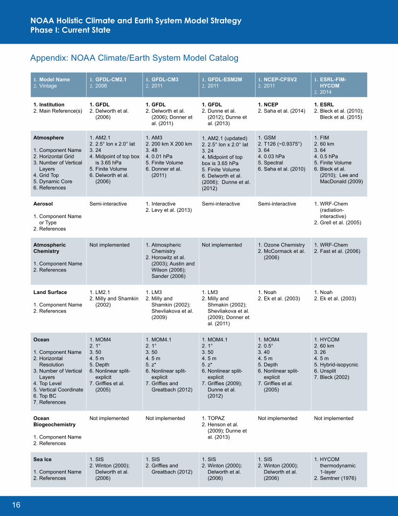
1. Model Name2. Vintage

1. GFDL-CM2.12. 2006

1. GFDL-CM32. 2011

1. GFDL-ESM2M2. 2011

1. NCEP-CFSV22. 2011

1. ESRL-FIM-HYCOM

2. 2014

1. Institution 2. Main Reference(s)

1. GFDL2. Delworth et al.

(2006)

1. GFDL2. Delworth et al.

(2006); Donner et al. (2011)

1. GFDL2. Dunne et al.

(2012); Dunne et al. (2013)

1. NCEP2. Saha et al. (2014)

1. ESRL2. Bleck et al. (2010);

Bleck et al. (2015)

Atmosphere

1. Component Name2. Horizontal Grid3. Number of Vertical

Layers4. Grid Top5. Dynamic Core6. References

1. AM2.12. 2.5° lon x 2.0° lat3. 244. Midpoint of top box

is 3.65 hPa5. Finite Volume6. Delworth et al.

(2006)

1. AM32. 200 km X 200 km3. 484. 0.01 hPa5. Finite Volume6. Donner et al.

(2011)

1. AM2.1 (updated)2. 2.5° lon x 2.0° lat3. 244. Midpoint of top box is 3.65 hPa5. Finite Volume6. Delworth et al. (2006); Dunne et al. (2012)

1. GSM2. T126 (~0.9375°)3. 644. 0.03 hPa5. Spectral6. Saha et al. (2010)

1. FIM2. 60 km3. 644. 0.5 hPa5. Finite Volume 6. Bleck et al.

(2010); Lee and MacDonald (2009)

Aerosol

1. Component Name or Type

2. References

Semi-interactive 1. Interactive2. Levy et al. (2013)

Semi-interactive Semi-interactive 1. WRF-Chem (radiation-interactive)

2. Grell et al. (2005)

Atmospheric Chemistry

1. Component Name2. References

Not implemented 1. Atmospheric Chemistry

2. Horowitz et al. (2003); Austin and Wilson (2006); Sander (2006)

Not implemented 1. Ozone Chemistry2. McCormack et al.

(2006)

1. WRF-Chem2. Fast et al. (2006)

Land Surface


1. LM2.12. Milly and Shamkin

(2002)

1. LM32. Milly and

Shamkin (2002); Shevliakova et al. (2009)

1. LM32. Milly and

Shmakin (2002); Shevliakova et al. (2009); Donner et al. (2011)

1. Noah2. Ek et al. (2003)

1. Noah2. Ek et al. (2003)

Ocean

1. Component Name2. Horizontal

Resolution3. Number of Vertical

Layers4. Top Level5. Vertical Coordinate6. Top BC7. References

1. MOM42. 1°3. 504. 5 m5. Depth6. Nonlinear split-

explicit7. Griffies et al.

(2005)

1. MOM4.12. 1°3. 504. 5 m5. z*6. Nonlinear split-

explicit7. Griffies and

Greatbach (2012)

1. MOM4.12. 1°3. 504. 5 m5. z*6. Nonlinear split-

explicit7. Griffies (2009);

Dunne et al. (2012)

1. MOM42. 0.5°3. 404. 5 m5. Depth6. Nonlinear split-

explicit7. Griffies et al.

(2005)

1. HYCOM2. 60 km3. 264. 5 m5. Hybrid-isopycnic6. Unsplit7. Bleck (2002)

Ocean Biogeochemistry


Not implemented Not implemented 1. TOPAZ2. Henson et al.

(2009); Dunne et al. (2013)

Not implemented Not implemented

Sea Ice


1. SIS2. Winton (2000);

Delworth et al. (2006)

1. SIS2. Griffies and

Greatbach (2012)

1. SIS2. Winton (2000);


1. SIS2. Winton (2000);


1. HYCOM thermodynamic 1-layer

2. Semtner (1976)


Appendix: NOAA Climate/Earth System Model Catalog

17

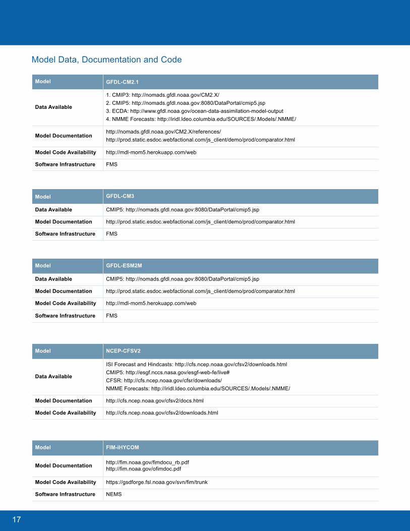
Model GFDL-CM2.1

Data Available

1. CMIP3: http://nomads.gfdl.noaa.gov/CM2.X/2. CMIP5: http://nomads.gfdl.noaa.gov:8080/DataPortal/cmip5.jsp3. ECDA: http://www.gfdl.noaa.gov/ocean-data-assimilation-model-output4. NMME Forecasts: http://iridl.ldeo.columbia.edu/SOURCES/.Models/.NMME/

Model Documentationhttp://nomads.gfdl.noaa.gov/CM2.X/references/http://prod.static.esdoc.webfactional.com/js_client/demo/prod/comparator.html

Model Code Availability http://mdl-mom5.herokuapp.com/web

Software Infrastructure FMS

Model GFDL-CM3

Data Available CMIP5: http://nomads.gfdl.noaa.gov:8080/DataPortal/cmip5.jsp

Model Documentation http://prod.static.esdoc.webfactional.com/js_client/demo/prod/comparator.html


Model GFDL-ESM2M

Data Available CMIP5: http://nomads.gfdl.noaa.gov:8080/DataPortal/cmip5.jsp

Model Documentation http://prod.static.esdoc.webfactional.com/js_client/demo/prod/comparator.html

Model Code Availability http://mdl-mom5.herokuapp.com/web


Model NCEP-CFSV2

Data Available

ISI Forecast and Hindcasts: http://cfs.ncep.noaa.gov/cfsv2/downloads.htmlCMIP5: http://esgf.nccs.nasa.gov/esgf-web-fe/live#CFSR: http://cfs.ncep.noaa.gov/cfsr/downloads/NMME Forecasts: http://iridl.ldeo.columbia.edu/SOURCES/.Models/.NMME/

Model Documentation http://cfs.ncep.noaa.gov/cfsv2/docs.html

Model Code Availability http://cfs.ncep.noaa.gov/cfsv2/downloads.html

Model FIM-iHYCOM

Model Documentation http://fim.noaa.gov/fimdocu_rb.pdf http://fim.noaa.gov/ofimdoc.pdf

Model Code Availability https://gsdforge.fsl.noaa.gov/svn/fim/trunk

Software Infrastructure NEMS

Model Data, Documentation and Code

https://gsdforge.fsl.noaa.gov/svn/fim/trunk

18

ReferencesAbhilash, S., and A. K. Sahai, S. Pattnaik, B. N. Goswami, and A. Kumar, 2014: Extended range prediction of active-break spells of Indian summer monsoon rainfall using an ensemble prediction system in NCEP Climate Forecast System. Int. J. Climatol., 34, 98–113. doi:10.1002/joc.3668

Adcroft, A., and J. M. Campin, 2004: Rescaled height coordinates for accurate representation of free-surface flows in ocean circulation models. Ocean Modell., 7, 269–284.

Adcroft, A., 2014: Next generation ocean and sea-ice models. GFDL 2014 Lab Review. [Available online at http://www.gfdl.noaa.gov/cms-filesystem-action/administrative/2014review/presentations/04.adcroft_review2014.pdf.].

Anderson, J. L., and Coauthors, 2004: The new GFDL atmosphere and land model AM2-LM2: Evaluation with prescribed SST simulations. J. Climate, 17, 4641–4673.

Austin, J., and R. J. Wilson, 2010: Sensitivity of polar ozone to sea surface temperature and halogen amounts. J. Geophys. Res., 115, D18303, doi:10.1029/2009JD013292.

Austin, J., D. M. Schwarzkopf, R. J. Wilson, and H. Levy II, 2013: Stratospheric ozone and temperature simulated from the preindustrial era to present day. J. Climate, 26, 3528–3543.

Barker, H. W., R. Pincus, and J.-J. Morcrette, 2002: The Monte Carlo independent column approximation. Extended Abstracts, GCSS-ARM Workshop on the Representation of Cloud Systems in Large-Scale Models, Kananaskis, AB, Canada, GEWEX, 1–10.

Becker, E., H. van den Dool, and Q. Zhang, 2014: Predictability and forecast skill in NMME. J. Climate, 27, 5891–5906.

Bleck, R., 2002: An oceanic general circulation model framed in hybrid isopycnic-Cartesian coordinates. Ocean Modell., 4, 55–88.

Bleck, R., S. Benjamin, J. Lee, and A. E. MacDonald, 2010: On the use of an adaptive, hybrid-isentropic vertical coordinate in global atmospheric modeling. Mon. Wea. Rev., 138, 2188–2210.

Bleck, R., J.-W. Bao, S.G. Benjamin, J.M. Brown, M. Fiorino, T. Henderson, J.-L. Lee, A.E. MacDonald, P. Madden, J. Middlecoff, J. Rosinski, T.G. Smirnova, S. Sun, N. Wang, 2015: A vertically flow-following, icosahedral-grid model for medium-range and seasonal prediction. Part 1: Model description. Mon. Wea. Rev., submitted.

Bleck, R., and S. Sun, 2012: iHYCOM Documentation. [Available online at http://fim.noaa.gov/ofimdoc.pdf.].

Bollasina, M. A., Y. Ming, and V. Ramaswamy, 2013: Earlier onset of the Indian monsoon in the late twentieth century. Geophys. Res. Lett., 40, 715–720.

Bollasina, M. A., Y. Ming, V. Ramaswamy, M. D. Schwarzkopf, and V. Naik, 2014: Contribution of local and remote anthropogenic aerosols to the twentieth century weakening of the South Asian Monsoon. Geophys. Res. Lett., 41, 680–687, doi:10.1002/2013GL058183.

Bretherton, C. S., J. R. McCaa, and H. Grenier, 2004: A new parameterization for shallow cumulus convection and its application to marine subtropical cloud-topped boundary layers. Part I: Description and 1D results. Mon. Wea. Rev., 132, 864–882.

Clough, S. A., and Coauthors, 2005: Atmospheric radiative transfer modeling: A summary of the AER codes. J. Quant. Spectrosc. Radiat. Transfer, 91, 233–244.

Collela, P., and P. R. Woodward, 1984: The Piecewise Parabolic Method (PPM) for gas-dynamical simulations. J. Comput. Phys., 54, 174–201.

Cummings, J. A., 2005: Operational multivariate ocean data assimilation. Q.J.R. Meteorol. Soc., 131, 3583–3604.

Danabasoglu, G., and Coauthors, 2006: Diurnal coupling in the tropical oceans of CCSM3. J. Climate, 19, 2347–2365.

Delworth, T. L., and Coauthors, 2006: GFDL’s CM2 global coupled climate models. Part I: Formulation and simulation characteristics. J. Climate, 19, 643–674.

Delworth, T. L., and Coauthors, 2012: Simulated climate and climate change in the GFDL CM2.5 high-resolution coupled climate model. J. Climate, 25, 2755–2781.

Delworth, 2014: Simulating regional hydroclimate variability and change on decadal scales. GFDL 2014 Lab Review. [Available online at http://www.gfdl.noaa.gov/cms-filesystem-action/administrative/2014review/presentations/09.delworth_session_5%282%29.pdf.]

Derber, J., and A. Rosati, 1989: A global oceanic data assimilation system. J. Phys. Oceanog., 19, 1333–1347.

Donner, L. J., 1993: A cumulus parameterization including mass fluxes, vertical momentum dynamics, and mesoscale effects. J. Atmos. Sci., 50, 889–906.

Donner, L. J., C. J. Seman, R. S. Hemler, and S. Fan, 2001: A cumulus parameterization including mass fluxes, convective vertical velocities, and mesoscale effects: Thermodynamic and hydrological aspects in a general circulation model. J. Climate, 14, 3444–3463.

Donner, L. J., and Coauthors, 2011: The dynamical core, physical parameterizations, and basic simulation characteristics of the atmospheric component AM3 of the GFDL coupled model CM3. J. Climate, 24, 3484–3519.

Dunne, J., and Coauthors, 2012a: GFDL’s ESM2 global coupled climate-carbon earth system models. Part I: Physical formulation and baseline simulation characteristics. J. Climate, 25, 6646–6665.

Dunne, J. P., J. R. Toggweiler, and B. Hales, 2012b: Global calcite cycling constrained by sediment preservation controls. Global Biogeochem. Cycles, 26, GB303, doi:10.1029/2010GB003935.

Dunne, J., and Coauthors, 2013: GFDL’s ESM2 global coupled climate-carbon earth system models. Part II: Carbon system formulation and baseline simulation characteristics. J. Climate, 26, 2247–2267.

Dunne, J., 2014: Chemistry, carbon, ecosystems, and climate: Coupled Carbon-climate Earth System Modeling. GFDL 2014 Lab Review. [Available from http://www.gfdl.noaa.gov/cms-filesystem-action/administrative/2014review/presentations/01.esm_jpd_20140508_final.pdf .].

Ek, M. B., and Coauthors, 2003: Implementation of Noah land surface model advances in the National Centers for Environmental Prediction operational mesoscale Eta model. J. Geophys. Res., 108, 8851, doi:1029/2002JD003296.

Ferrari, R., S. Griffith, A. Nurser, and G. Vallies, 2010: A boundary-value problem for the parameterized mesoscale eddy transport. Ocean Modell., 32, 143–156.

Fox-Kemper, B., and Coauthors, 2011: Parameterization of mixed layer eddies. III: Implementation and impact in global ocean climate simulations. Ocean Modell., 39, 61–78.

Freidenreich, S. M., and V. Ramaswamy, 1999: A new multiple-band solar radiative parameterization for general circulation models. J. Geophys. Res., 104, 389–409.

Geider, R. J., J. L. MacIntyre, and T. M. Kana, 1997: A dynamic model of phytoplankton growth and acclimation. Responses of the balanced growth rate and chlorophyll: Carbon ratio to light, nutrient-limitation, and temperature. Mar. Ecol. Prog. Ser., 148, 187–200.

Gent, P., and J. C. McWilliams, 1990: Isopycnal mixing in ocean circulation models. J. Phys. Oceanogr., 31, 2273–2279.

Gent, P. R., J. Willebrand, T. J. McDougall, and J. C. McWilliams, 1995: Parameterizing eddy-induced tracer transports in ocean circulation models. J. Phys. Oceanogr., 25, 463–474.

Ghan, S. J., L. R. Leung, R. C. Easter, and H. Abdul-Razzak, 1997: Prediction of cloud droplet number in a general circulation model. J. Geophys. Res., 102, 777–794.

Gnanadesikan, A., and Coauthors, 2006: GFDL’s global coupled climate models. Part II: The baseline ocean simulation. J. Climate, 19, 675–697.

Golaz, C., 2014: Towards the next generation GFDL global atmospheric model. GFDL 2014 Lab Review. [Available online at http://www.gfdl.noaa.gov/cms-filesystem-action/administrative/2014review/presentations/02.golaz_review2014.pdf]

Govett, M., 2010: The Scalable Modeling System – SMS. [Available online at http://www.esrl.noaa.gov/gsd/ab/ac/sms.html.].

Grell, G. A., and S. R. Freitas, 2014: A scale- and aerosol-aware stochastic convective parameterization for weather and air quality modeling. Adv. Comp. Phys., 14, 5233–5250.

Griffies, S. M., 1998: The Gent-McWilliams skew flux. J. Phys. Oceanogr., 28, 831–841.

Griffies, S. M., and Coauthors, 1998: Isoneutral diffusion in a z-coordinate ocean model. J. Phys. Oceanogr., 28, 805–830.

Griffies, S. M., and R. W. Hallberg, 2000: Biharmonic friction with a Smagorinsky-like viscosity for use in large-scale eddy-permitting ocean models. Mon. Wea. Rev., 128, 2935–2946.

Griffies, S. M., M. J. Harrison, R. C. Pacanowski, and A. Rosati, 2004: Technical guide to MOM4. GFDL Ocean Group Technical Report No 5, 337 pp. [Available online at http://www.gfdl.noaa.gov/~fms]

Griffies, and Coauthors, 2005: Formulation of an ocean model for global climate simulations. Ocean Sci., 1, 45–70.

Griffies, S. M., 2010: Elements of MOM4P1. GFDL Ocean Group Tech. Rep. 6, NOAA/Geophysical Fluid Dynamics Laboratory, 444 pp. [Available online at http://www.gfdl.noaa.gov/fms.].

Griffies, S. M., and Coauthors, 2011: The GFDL CM3 coupled climate model: Characteristics of the ocean and ice simulation. J. Climate, 24, 3520–3544.

Held, I., 2014: Model development for GFDL’s next generation climate and earth system models. GFDL 2014 Lab Review. [Available online at http://www.gfdl.noaa.gov/cms-filesystem-action/administrative/2014review/presentations/01.held_review2014.pdf]

Hoerling, M. P., and Co-authors, 2013: Anatomy of an extreme event. J. Climate, 26, 2811–2832.

Hoffman, F. M., and Coauthors, 2013: Causes and implications of persistent atmospheric carbon dioxide biases in Earth System Models. J. Geophys. Res. Biogeosci., 119, 141–162.

Hong, S.-Y., and H.-L. Pan, 1996: Nonlocal boundary layer vertical diffusion in a medium-range forecast model. Mon. Wea. Rev., 124, 2322–2339.

Hong, S.-Y., and H.-L. Pan, 1998: Convective trigger function for a mass-flux cumulus parameterization scheme. Mon. Wea. Rev., 126, 2599–2620.

Horowitz, L. W., and Coauthors, 2003: A global simulation of tropospheric ozone and related tracers: Description and evaluation of MOZART, version 2. J. Geophys. Res., 108, 4784, doi:10.1029/2002JD002853.

Horowitz, L. W., and Coauthors, 2007: Observational constraints on the chemistry of isoprene nitrates over the eastern United States. J. Geophys. Res., 112, D12508, doi:10.1029/2006JD007747.

Hu, Z., A. Kumar, B. Huang, J. Shu, and Y. Guan, 2014: Prediction skill of North Pacific variability in NCEP Climate Forecast System Version 2: Impact of ENSO and beyond. J. Climate, 27, 4263–4272.

Hundsdorfer, W., and R. Trompert, 1994: Method of lines and direct discretization: A comparison for linear advection. Appl. Numer. Math., 13, 469–490.

Hunke, E. C., and J. K. Duckowicz, 1997: An elastic-viscous-plastic model for sea ice dynamics. J. Phys. Oceanogr., 27, 1849–1867.

Hunyh, H. T., 1996: Schemes and constraints for advection. Fifteenth International Conference on Numerical Methods in Fluid Dynamics, P. Kutler, J. Flores, and J.-J. Chattor, Eds., Lecture Notes in Physics, 490, Springer, 498–503.

Iacona, M. J., E. J. Mlawer, S. A. Clough, and J.-J. Morcrette, 2000: Impact of an improved longwave radiation model, RRTM, on the energy budget and thermodynamic properties of the NCAR Community Climate Model, CCM3. J. Geophys. Res., 105, 873–890.

Jia, L., and Coauthors, 2015: Improved seasonal prediction of temperature and precipitation over land in a high-resolution GFDL climate model. J. Climate, 28, 2044–2062.

John, J. G., A. M. Fiore, V. Naik, L. Horowitz, and J. P. Dunne, 2012: Climate versus emission drivers of methane lifetime against loss by tropospheric OH from 1860–2100. Atmos. Chem. Phys., 12, 21–36.


19

Kapnick, S. B., and T. L. Delworth, 2013: Controls of global snow under a changed climate. J. Climate, 26, 5537–5562.

Kapnick, S. B., 2014: Prediction of Regional Hydrology and Snowpack. GFDL 2014 Lab Review. [Available online at http://www.gfdl.noaa.gov/cms-filesystem-action/administrative/2014review/presentations/04.kapnick_theme_5.pdf]

Kirtman, B. P., and Coauthors, 2014: The North American Multi-model Ensemble. Phase-I: Seasonal-to-interannual prediction; Phase-2: Toward developing intraseasonal prediction. Bull. Amer. Meteor. Soc., 95, 585–601.

Knutti, R., D. Masson, and A. Gettelman, 2013: Climate model genealogy: Generation CMIP5 and how we got there. Geophys. Res. Lett., 40, 1194–1199.

Kristiansen, T., C. Stock, K. F. Drinkwater, and E. N. Curchitser, 2014: Mechanistic insights into the effects of climate change on larval cod. Global Change Biology, 20, 1559–1584. doi:10.1111/gcb.12489.

Large, W. G., J. C. McWilliams, and S. C. Doney, 1994: Oceanic vertical mixing: A review and a model with a nonlocal boundary mixing parameterization. Rev. Geophys., 32, 363–403.

Large, W. G., G. Danabasoglu, J. C. McWilliams, P. R. Gent, and F. O. Bryan, 2001: Equatorial circulation of a global ocean climate model with anisotropic horizontal viscosity. J. Phys. Oceanogr., 31, 518–536.

Lee, H.-C., A. Rosati, and M. J. Spelman, 2006: Barotropic tidal mixing effects in a coupled climate model: Oceanic conditions in the North Atlantic. Ocean Modell., 11, 467–477.

Lee, J. L., and A. E. MacDonald, 2009: A finite-volume icosahedral shallow-water model on a local coordinate. Mon. Wea. Rev., 137, 1422–1437.

Marshall, J., C. Hill, L. Perelman, and A. Adcroft, 1997: Hydrostatic, quasi-hydrostatic, and non-hydrostatic ocean modeling. J. Geophys. Res., 102 (C3), 5733–5752.

McDougall, T. J., and W. K. Dewar, 1998: Vertical mixing and cabbeling in layered models. J. Phys. Oceanogr., 28, 1458–1480.

Milly, P. C. D., and A. B. Shmakin, 2002: Global modeling of land water and energy balances. Part I: The land dynamics (LaD) model. J. Hydrometeor., 3, 283–299.

Milly, P. C. D., and Coauthors, 2014a: An enhanced model of land water and energy for global hydrological and earth-system studies. J. Hydrometeor., 15, 1739–1761.

Milly, P. C. D., 2014b: Hydrology. GFDL 2014 Lab Review. [Available online at http://www.gfdl.noaa.gov/cms-filesystem-action/administrative/2014review/presentations/05.milly%20upload%202.pdf.].

Ming, Y., V. Ramaswamy, L. J. Donner, and V. T. J. Phillips, 2006: A robust parameterization of cloud droplet activation. J. Atmos. Sci., 63, 1348–1356.

Mlawer, E. J., S. J. Taubman, P. D. Brown, M. J. Iacono, and S. A. Clough, 1997: Radiative transfer for inhomogeneous atmosphere: RRTM, a validated correlated-k model for the longwave. J. Geophys. Res., 102 (D14), 663–682.

Moorthi, S., and M. J. Suarez, 1992: Relaxed Arakawa-Schubert: A parameterization of moist convection for general circulation models. Mon. Wea. Rev., 120, 978–1002.

Morel, A., and D. Antoine, 1994: Heating rate within the upper ocean in relation to its bio-optical state. J. Phys. Oceanogr., 24, 1652–1665.

Msadek, R., G. A. Vecchi, M. Winton, and R. Gudgel, 2014: Importance of initial conditions in seasonal predictions of Arctic sea ice extent. Geophys. Res. Lett., 41, 5208–5215,

Murray, R. J., 1996: Explicit generation of orthogonal grids for ocean models. J. Comput. Phys., 126, 251–273.

Naik, V., and Coauthors, 2013: Impact of preindustrial to present-day changes in short-lived pollutant emissions on atmospheric composition and climate forcing. J. Geophys. Res., 118, 86–110.

Naik, V., 2014: Chemistry-Climate Interactions. GFDL 2014 Lab Review. [Available online at http://www.gfdl.noaa.gov/cms-filesystem-action/administrative/2014review/presentations/02.van.gfdl_review2014_uploaded.pdf.].

National Research Council, 2012. A National Strategy for Advancing Climate Modeling. Washington, DC. National Academy Press. [Available on line at http://www.nap.edu/catalog.php?record_id=13430.]

Pan, J.-L., and W.-S. Wu, 1995: Implementing a mass flux convective parameterization package for the NMC medium range forecast model. NMC Office Note 409, 40 pp. [Available online at www.emc.ncep.noaa.gov/officenotes/FullTOC.html#1990].

Peng, P., A. Kumar, H. van den Dool, and A. G. Barnston, 2002: An analysis of multi-model ensemble predictions for seasonal climate anomalies. J. Geophys. Res., 107, D24, 10.1029/2002JD002712.

Peng, P., A. G., Barnston, and A. Kumar, 2013: A comparison of skill among two versions of NCEP climate forecast system (CFS) and CPC’s operational short-lead seasonal outlooks. Wea. Forecasting, 28, 445–462.

Pincus, R., H. W. Barker, and J.-J. Morcrette, 2003: A fast, flexible, approximate technique for computing radiative transfer in inhomogeneous cloud fields. J. Geophys. Res., 108, 4376, doi:10.1029/2002JD003322.

Polovina, J. J., J. P. Dunne, P. A. Woodworth, and E. A. Howell, 2011: Projected expansion of the subtropical biome and contraction of the temperate and equatorial upwelling biomes in the North Pacific under global warming. ICES. J. Mar. Sci., 68, 986–995.

Putnam, W. M., and S. J. Lin, 2007: Finite-volume transport on various cubed-sphere grid. J. Comput. Phys., 227, 55–79.

Reichler, T., and J. Kim, 2008: How well do coupled models simulate today’s climate?. Bull. Amer. Meteor. Soc., 89, 303–311. doi:10.1175/BAMS-89-3-303.

Riddle, E., A. H. Butler, J. Furtado, J. L. Cohen, and A. Kumar, 2013: CFSv2 ensemble prediction of the wintertime arctic oscillation. Clim. Dyn., 41, 1099–1116. doi:10.1007/s00382-013-1850-5.

Rotstayn, L. D., 1997: A physically based scheme for the treatment of stratiform clouds and precipitation in large-scale models. I: Description and evaluation of microphysical processes. Quart. J. Roy. Meteorol. Soc., 123, 1227–1282.

Rotstayn, L. D., B. F. Ryan, and J. Katzfey, 2000: A scheme for calculation of the liquid fraction in mixed-phase clouds in large-scale models. Mon. Wea. Rev., 128, 1070–1088.

aczewski, R. R., and J. P. Dunne, 2010: Enhanced nutrient supply to the California Current Ecosystem with global warming and increased stratification in an earth system model. Geophys. Res. Lett., 37, L21606, doi:10.1029/2010GL045019.

Saba, V. S., and C. A. Stock, 2012: Projected response of an endangered marine turtle population to climate change. Nature Climate Change, 2, doi:10.1038/nclimate1582.

Saha, S., and Coauthors, 2010: The NCEP Climate Forecast System Reanalysis. Bull. Amer. Meteor. Soc., 91, 1015–1057.

Saha, S., and Coauthors, 2014: The NCEP climate forecast system version 2. J. Climate, 27, 2185–2208.

Schwarzkopf, M. D., and V. Ramaswamy, 1999: Radiative effects of CH4, N2O, halocarbons, and the foreign-broadened H2O continuum: A GCM experiment. J. Geophys. Res., 104, 467–488.

Semtner, A. J., 1976: A model for the thermodynamic growth of sea ice in numerical investigations of climate. J. Phys. Oceanogr., 6, 27–37.

Shevliakova, E., and Coauthors, 2009: Carbon cycling under 300 years of land use change: Importance of the secondary vegetation sink. Global Biogeochem. Cycles, 23, GB2022, doi:10.1029/2007GB003176.

Shevliakova, E., 2014: Land Ecosystems-Climate Interactions. GFDL 2014 Lab Review. [Available online at http://www.gfdl.noaa.gov/cms-filesystem-action/administrative/2014review/presentations/05.shevliakova_review_v3.pdf.].

Simmons, H. L., S. R. Jayne, L. C. St. Laurent, and A. J. Weaver, 2004: Tidally driven mixing in a numerical model of the ocean general circulation. Ocean Modell., 6, 245–263.

Smagorinsky, J., 1993: Some historical remarks on the use of non-linear viscosities. Large Eddy Simulation of Complex Engineering and Geophysical Flows, B. Galperin and S. A. Orszag, Eds., Cambridge University Press, 3–36.Stacey, M., W. S. Pond, and Z. P. Nowak, 1995: A numerical model of the circulation in Knight Inlet, British Columbia, Canada. J. Phys. Oceanogr., 25, 1037–1062.

Stock, C. A., J. P. Dunne, and J. John, 2014: Global-scale carbon and energy flows through the marine food web: an analysis with a coupled physical-biological mode. Progress in Oceanography, 120, doi:10.1016/j.pocean.2013.07.001.

Stock, C., 2014: Connecting climate and marine ecosystems. GFDL 2014 Lab Review. [Available from http://www.gfdl.noaa.gov/cms-filesystem-action/administrative/2014review/presentations/06.stock_review_final.pdf.].

Sweby, P., 1994: High-resolution schemes using the flux limiters for hyperbolic conservation laws. SIAM J. Numer. Anal., 21, 995–1101.

Tiedtke, M., 1993: Representation of clouds in large-scale models. Mon. Wea. Rev., 121, 3040–3061.

van Oldenburgh, G., S. Y. Phillip, and M. Collins, 2005: El Nino in a changing climate: A multi-model study. Ocean Sci., 1, 85–95.

Vancoppenolle, M. L., and Coauthors, 2013: Future Arctic Ocean primary productivity from CMIP5 simulations: Uncertain outcome, but consistent mechanisms. Glob. BioGeo. Cyc., 27, 605–619.

Vecchi, G. A., 2014a: Understanding and predicting regional water and extremes. GFDL 2014 Lab Review. [Available from http://www.gfdl.noaa.gov/cms-filesystem-action/administrative/2014review/presentations/01.vecchi_intro_prediction_final.pdf.].

Vecchi, G. A., and Coauthors, 2014b: On the seasonal forecasting of regional tropical cyclone activity. J. Climate, 27, 7994–8016.

Wang, W., M. Chen, and A. Kumar, 2013: Seasonal prediction of Arctic sea ice extent from a coupled dynamical forecast system. Clim. Dyn., 41, 1375–1394.

Wang, W., M.-P. Hung, S. J. Weaver, A. Kumar, and X. Fu, 2014: MJO prediction in the NCEP Climate Forecast System version 2. Clim. Dyn., 42, 2509–2520.

Weaver, S., A. Kumar, and M. Chen, 2014: Recent increases in extreme temperature occurrence over land. Geophys. Res. Lett., doi:10.1002/2014GL060300.

Wilcox, E. M., and L. J. Donner, 2007: The frequency of extreme rain events in satellite rain-rate estimates and an atmospheric general circulation model. J. Climate, 20, 53–69.

Winton, M., 2000: A reformulated three-layer sea ice model. J. Atmos. Oceanic. Technol., 17, 525–531.

Winton, M., A. Adcroft, S. M. Griffies, R. W. Hallberg, L. W. Horowitz, and R. J. Stouffer, 2013: Influence of ocean and atmosphere components on simulated climate sensitivities. J. Climate, 26, doi:10.1175/JCLI-D-12-00121.1.

Wittenberg, A. T., 2014: ENSO predictability and dynamics. GFDL 2014 Lab Review. [Available online at http://www.gfdl.noaa.gov/cms-filesystem-action/administrative/2014review/presentations/08.wittenberg_enso_session_5_presentation.pdf.].

Xue, Y., M. Chen, A. Kumar, Z.-Z. Hu, and W. Wang, 2013: Prediction skill and bias of tropical Pacific sea surface temperature in the NCEP Climate Forecast System Version 2. J. Climate, 26, 5358–5378.

Zhang, S., M. J. Harrison, A. Rosati, and A. T. Wittenberg, 2007: System design and evaluation of coupled ensemble data assimilation for global oceanic climate studies. Mon. Wea. Rev., 138, 3905–3931.

Zhao, M., I. M. Held, S.-J. Lin, and G. A. Vecchi, 2009: Simulations of global hurricane climatology, interannual variability, and response to global warming using a 50-km resolution GCM. J. Climate, 22, 6653–6678.

20

NOAA Technical Report OAR CPO-3

NOAA Holistic Climateand Earth SystemModel StrategyPhase I: Current Statedoi:10.7289/V5Z31WKK

Documents

NOAA Holistic Climate and Earth System Model Strategy Phase I