Embed Size (px)
Citation preview

ee.sharif.edu/~dip
E. Fatemizadeh, Sharif University of Technology, 2011
1
Digital Image Processing
Image Compression
1
• Goal:
– Reducing the amount of data required to represent a digital image.
• Transmission
• Archiving
– Mathematical Definition: • Transforming a 2-D pixel array into a statistically uncorrelated data
set.

ee.sharif.edu/~dip
E. Fatemizadeh, Sharif University of Technology, 2011
2
Digital Image Processing
Image Compression
2
• Two Main Category:
– Lossless: TIFF (LZW,ZIP)
– Lossy: JPEG and JPEG2000
ee.sharif.edu/~dip
E. Fatemizadeh, Sharif University of Technology, 2011
3
Digital Image Processing
Image Compression
3
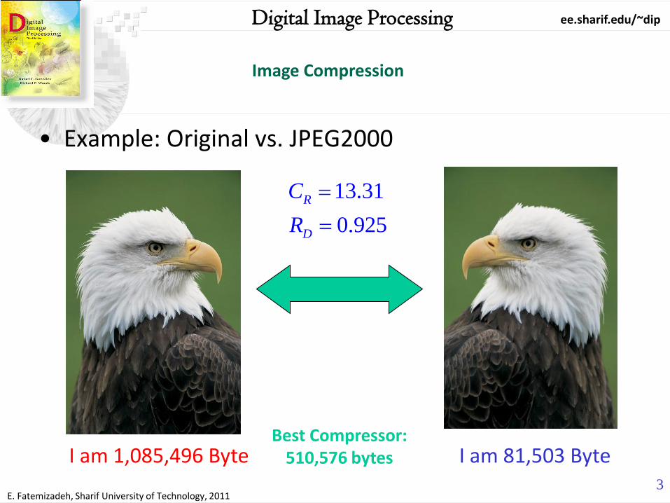
• Example: Original vs. JPEG2000
I am 1,085,496 Byte I am 81,503 Byte
13.31
0.925
R
D
C
R
Best Compressor: 510,576 bytes

ee.sharif.edu/~dip
E. Fatemizadeh, Sharif University of Technology, 2011
4
Digital Image Processing
Image Compression
4
• Fundamentals:
– Raw image: A set of n1bits
– Compressed image: A set of n2 bits.
– Compression ratio:
– Relative Data Redundancy in A:
– Example: n1= 100KB and n2 = 10Kb, then C0 = 10 , and RD = 90%
• Special cases: 1) n1>>n2 → CR ≈ ∞, RD ≈ 1
• 2) n1 ≈ n2 → CR ≈ 1, RD ≈ 0
• 3) n1 << n2 → CR ≈ 0, RD ≈ -∞
1
2
R
nC
n
11D
R
RC

ee.sharif.edu/~dip
E. Fatemizadeh, Sharif University of Technology, 2011
5
Digital Image Processing
Image Compression
5
• Three basic data redundancies:
– Coding redundancy
– Spatial/Temporal (Inter-Pixel) redundancy,
– Irrelevant/Psycho-Visual redundancy.

ee.sharif.edu/~dip
E. Fatemizadeh, Sharif University of Technology, 2011
6
Digital Image Processing
Image Compression
6
• Coding redundancy:
– Type of coding (# of bits for each gray level)
– Image histogram: • rk: Represents the gray levels of an image
• pr(rk): Probability of occurrence of rk
• l(rk): Number of bits used to represent each rk.
• Lavg: Average # of bits required to represent each pixel:
( ) 0,1,2,..., 1kr k
np r k L
n
1
0
( ) ( )L
avg k r k
k
L l r p r

ee.sharif.edu/~dip
E. Fatemizadeh, Sharif University of Technology, 2011
7
Digital Image Processing
Image Compression
7
• Example (1): Variable Length Coding
1
2
= 0.25(2)+0.47(1)+0.25(3)+0.03(3)=1.81 bits
Code 2: 256 256 8 8 14.42 1 0.774 77.4%
256 256 1.81 1.81 4.42
avg
R D
L
nC R
n

ee.sharif.edu/~dip
E. Fatemizadeh, Sharif University of Technology, 2011
8
Digital Image Processing
Image Compression
8
• Example (2): Spatial Redundancy
– Uniform intensity
– Highly correlated in horizontal direction
– No correlation in vertical direction
– Coding using run-length pairs:
1 1 2 2, , , ,g RL g RL

ee.sharif.edu/~dip
E. Fatemizadeh, Sharif University of Technology, 2011
9
Digital Image Processing
Image Compression
9
• Irrelevant/Psychovisual Redundancy:
– Human perception of images: • Normally does NOT involve quantitative analysis of every pixel
value.
– Quantization eliminates psychovisual redundancy

ee.sharif.edu/~dip
E. Fatemizadeh, Sharif University of Technology, 2011
10
Digital Image Processing
Image Compression
10
• Image Compression using Psychovisual Redundancy:
– A Simple method: Discard lower order bits (4)
– IGS (Improved Gray Scale) Quantization: • Eye sensitivity to edges.
• Add a pseudo random number (lower order bits of neighbors) to central pixel and then discard lower order bits.
169 ÷ 16 = 10.56
167 ÷ 16 = 10.43
11
10
11 × 16 = 176
10 × 16 = 160
Rounded
values

ee.sharif.edu/~dip
E. Fatemizadeh, Sharif University of Technology, 2011
11
Digital Image Processing
Image Compression
11
Pixel Gray Level SUM IGC
i-1 N/A 0000 0000 N/A
i 0110 1100 0110 1100 0110
i+1 1000 1011 1001 0111 1001
i+2 1000 0111 1000 1110 1000
i+3 1111 0100 1111 0100 1111
• IGS Example:

ee.sharif.edu/~dip
E. Fatemizadeh, Sharif University of Technology, 2011
12
Digital Image Processing
Image Compression
12
• Sample Results: Original Simple Discard IGS

ee.sharif.edu/~dip
E. Fatemizadeh, Sharif University of Technology, 2011
13
Digital Image Processing
Image Compression
13
• Image information Measure:
– Self Information
1log log : m-ary units
2 for bit expression ( 0.5 1)
mI E P EP E
m P E I E

ee.sharif.edu/~dip
E. Fatemizadeh, Sharif University of Technology, 2011
14
Digital Image Processing
Image Compression
14
• Information Channel:
– A Source of statistically independent random events
– Discrete possible events with associated probability:
– Average information per source output (Entropy):
– For “zero-memory” (intensity source) imaging system: • Using Histogram
• This lower band of bits-length
1 2, , , Ja a a
1 2, , , JP a P a P a
1
logJ
j j
j
H P a P a
1
2
0
log /L
r k k k
k
H p r p r bits pixel

ee.sharif.edu/~dip
E. Fatemizadeh, Sharif University of Technology, 2011
15
Digital Image Processing
Image Compression
15
• Example:
1.6614 bits/pixelH

ee.sharif.edu/~dip
E. Fatemizadeh, Sharif University of Technology, 2011
16
Digital Image Processing
Image Compression
16
• Shannon First Theorem (Noiseless Coding Theorem):
– For a n-symbol group with Lavg, n average number of code symbol:
,
limavg n
n
LH
n

ee.sharif.edu/~dip
E. Fatemizadeh, Sharif University of Technology, 2011
17
Digital Image Processing
Image Compression
17
• Fidelity Criteria:
– Objective (Quantitative)
• A number (vector) is calculated
– Subjective (Qualitative)
• Judgment of different subject is used in limited level.

ee.sharif.edu/~dip
E. Fatemizadeh, Sharif University of Technology, 2011
18
Digital Image Processing
Image Compression
18
• Objective Criteria:
– :input image
– : approximated image
1 1
0 0
1 21 1 2
0 0
1 1 2
0 0
1 1 2
0 0
ˆ, , ,
1 ˆ , ,
1 ˆ , ,
ˆ ,
ˆ , ,
M N
abs
x y
M N
rms
x y
M N
x y
ms M N
x y
e x y f x y f x y
E f x y f x yMN
E f x y f x yMN
f x y
SNR
f x y f x y
ˆ ,f x y
,f x y

ee.sharif.edu/~dip
E. Fatemizadeh, Sharif University of Technology, 2011
19
Digital Image Processing
Image Compression
19
• Objective Criteria:
– PSNR: Peak SNR
2
10 1 1 2
0 0
10log1 ˆ , ,
: Maximum level of images (255 for 8bits)
M N
x y
LPSNR
f x y f x yMN
L

ee.sharif.edu/~dip
E. Fatemizadeh, Sharif University of Technology, 2011
20
Digital Image Processing
Image Compression
20
• Subjective Test

ee.sharif.edu/~dip
E. Fatemizadeh, Sharif University of Technology, 2011
21
Digital Image Processing
Image Compression
21
• Example:
– Original and three approximation. Erms=5.17
Erms=15.67
Erms=14.17

ee.sharif.edu/~dip
E. Fatemizadeh, Sharif University of Technology, 2011
22
Digital Image Processing
Image Compression
22
• Image Compression Model:
– Encoder: Create a set of symbols from image date.
• Source Encoder: Reduce input redundancy.
• Channel Encoder*: Increase noise immunity (noise robustness)
– Decoder: Construct output image from transmitted symbols
• Source Decoder: Reverse of Source encoder
• Channel Decoder*: Error detection/correction.
ee.sharif.edu/~dip
E. Fatemizadeh, Sharif University of Technology, 2011
23
Digital Image Processing
Image Compression
23
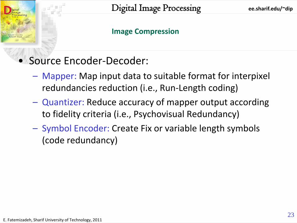
• Source Encoder-Decoder:
– Mapper: Map input data to suitable format for interpixel redundancies reduction (i.e., Run-Length coding)
– Quantizer: Reduce accuracy of mapper output according to fidelity criteria (i.e., Psychovisual Redundancy)
– Symbol Encoder: Create Fix or variable length symbols (code redundancy)

ee.sharif.edu/~dip
E. Fatemizadeh, Sharif University of Technology, 2011
24
Digital Image Processing
Image Compression
24
• Channel Encoder-Decoder*:
– Add controlled redundancy to source encoded data
– Increase noise robustness.
– Hamming (7-4) as an example:
3 2 1 0
4 2 1 4 2 1
1 3 2 1
7 6 5 3 0 1
1 1 3 5 7
2 3 1 0 2 2 3 6 7
4
2 3
4 5 6 74 2 1 0
4 bit binary input data:
7 bit binary output data:
Parity bits, Error check:
b b b b
h h h h h h
h b b b c h h h h
h b b b c h h h h
h h h h b b
c h h h hh b
b b
b b

ee.sharif.edu/~dip
E. Fatemizadeh, Sharif University of Technology, 2011
25
Digital Image Processing
Image Compression
25
• Image Compression Standards
• See Tables 8.3 and 8.4 for more details

ee.sharif.edu/~dip
E. Fatemizadeh, Sharif University of Technology, 2011
26
Digital Image Processing
Image Compression
26
• Error-Free Compression:
– ZIP, RAR, TIFF(LZW/ZIP)
• Compression Ratio: 2-10
– Steps:
• Alternative representation to reduce interpixel redundancy
• Coding the representation to reduce coding redundancy

ee.sharif.edu/~dip
E. Fatemizadeh, Sharif University of Technology, 2011
27
Digital Image Processing
Image Compression
27
• Variable-Length Coding:
– Variable-Length Coding
• Assign variable bit length to symbols based on its probability:
• Low probability (high information) more bits
• High Probability (low information) less bits

ee.sharif.edu/~dip
E. Fatemizadeh, Sharif University of Technology, 2011
28
Digital Image Processing
Image Compression
28
• Huffman Coding:
– Uses frequencies (Probability) of symbols in a string to build a variable rate prefix code.
– Each symbol is mapped to a binary string.
– More frequent symbols have shorter codes.
– No code is a prefix of another. (Uniquely decodable)
– It is optimum!
– CCITT, JBIG2, JPEG MPEG (1, 2, 4), H261-4

ee.sharif.edu/~dip
E. Fatemizadeh, Sharif University of Technology, 2011
29
Digital Image Processing
Image Compression
29
• Huffman Coding:
– Example:
• We have three symbols a, b, c, and c.

ee.sharif.edu/~dip
E. Fatemizadeh, Sharif University of Technology, 2011
30
Digital Image Processing
Image Compression
30
• Huffman Coding:
– A source string: aabddcaa
• Fixed Length Coding: 16 bits (ordinary coding)
– 00 00 01 11 11 10 00 00
• Variable length coding: 14bits (Huffman coding)
– 0 0 100 11 11 101 0 0
• Uniquely Decodable:
0 0 1 0 0 1 1 1 1 1 0 1 0 0
a a b d d c a a
ee.sharif.edu/~dip
E. Fatemizadeh, Sharif University of Technology, 2011
31
Digital Image Processing
Image Compression
31
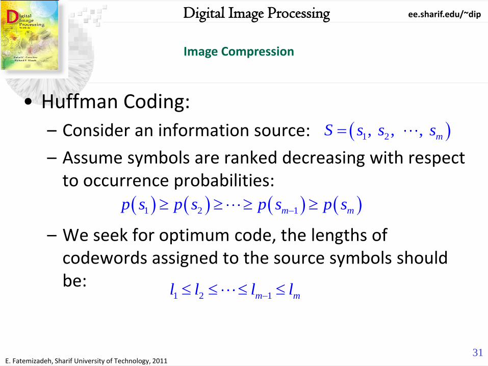
• Huffman Coding:
– Consider an information source:
– Assume symbols are ranked decreasing with respect to occurrence probabilities:
– We seek for optimum code, the lengths of codewords assigned to the source symbols should be:
1 2, , , mS s s s
1 2 1m mp s p s p s p s
1 2 1m ml l l l

ee.sharif.edu/~dip
E. Fatemizadeh, Sharif University of Technology, 2011
32
Digital Image Processing
Image Compression
32
• Huffman Coding: – Huffman (1951) Derived the following rules:
• Two least probable source symbols have equal-length codewords.
• These two codewords are identical except for the last bits, with binary 0 and 1, respectively.
• These source can be combined to form a new symbol. – Its occurrence probability is
– Its codeword is common prefix of order lm-1of the two codewords assigned to Sm and Sm-1 , respectively.
1 2 1m ml l l l
1m mP s P s

ee.sharif.edu/~dip
E. Fatemizadeh, Sharif University of Technology, 2011
33
Digital Image Processing
Image Compression
33
• Huffman Coding: – The new set of source symbols thus generated is referred to as the first
auxiliary source alphabet, which is one source symbol less than the original source alphabet.
– In the first auxiliary source alphabet, we can rearrange the source symbols according to a nonincreasing order of their occurrence probabilities.
– The same procedure can be applied to this newly created source alphabet.
– The second auxiliary source alphabet will again have one source symbol less than the first auxiliary source alphabet.
– This is repeated until we form a single source symbol with a probability of 1.
– Start from the source symbol in the last auxiliary source alphabet and trace back to each source symbol in original source alphabet to find the codewords.

ee.sharif.edu/~dip
E. Fatemizadeh, Sharif University of Technology, 2011
34
Digital Image Processing
Image Compression
34
• Huffman Coding:
– Source Reduction sequence.

ee.sharif.edu/~dip
E. Fatemizadeh, Sharif University of Technology, 2011
35
Digital Image Processing
Image Compression
35
g0.05
a b c d e f0.05 0.1 0.2 0.3 0.2 0.1
g0.05
a b c d e f0.05 0.1 0.2 0.3 0.2 0.1
0.1
g0.05
a b c d e f0.05 0.1 0.2 0.3 0.2 0.1
0.1 0.3
0.2 0.6
0.4
1.0
0
0
0
0
0
0
1
1
1
1
1
1
• More Illustration: Symbol Probability Codeword
a 0.05 0000
b 0.05 0001
c 0.1 001
d 0.2 01
e 0.3 10
f 0.2 110
g 0.1 111

ee.sharif.edu/~dip
E. Fatemizadeh, Sharif University of Technology, 2011
36
Digital Image Processing
Image Compression
36
2.2 bits/symbolavgL
• Example:

ee.sharif.edu/~dip
E. Fatemizadeh, Sharif University of Technology, 2011
37
Digital Image Processing
Image Compression
37
• Example:
– 8bits monochrome • Estimated Entropy: 7.3838 bits/pixel
– Huffman’s Coding: • MATLAB: 7.428 bits/pixel, CR = 1.077, RD = 0.0715

ee.sharif.edu/~dip
E. Fatemizadeh, Sharif University of Technology, 2011
38
Digital Image Processing
Image Compression
38
• Near Optimal

ee.sharif.edu/~dip
E. Fatemizadeh, Sharif University of Technology, 2011
39
Digital Image Processing
Image Compression
39
• Huffman drawbacks: – For large number symbols, construction of
optimal Huffman code is nontrivial.
– Huffman is block coding: • That is, some codeword having an integral number of
bits is assigned to a source symbol.
• A message may be encoded by cascading the relevant codewords. It is the block-based approach that is responsible for the limitations of Huffman codes.
• Computationally not efficient for a message with all possible symbols.

ee.sharif.edu/~dip
E. Fatemizadeh, Sharif University of Technology, 2011
40
Digital Image Processing
Image Compression
40
• Golomb Coding (1):
– Non-negative integer inputs
– Exponentially decaying probability distribution
– Inputs may be near optimal codes (simple than Huffman)
– JPEG-LS and AVS
– Notation: : Largest integer less than or equal to ,
:Smallest integer greater than or equal to ,
x x Floor
x x Ceil

ee.sharif.edu/~dip
E. Fatemizadeh, Sharif University of Technology, 2011
41
Digital Image Processing
Image Compression
41
• Golomb Coding (2):
– Goal: • Golomb Coding of n (Non-Negative) with respect to m>0:Gm(n)
– Combination of unary coding quotient and binary representation of remainder “n mod m”
– Unary coding of integer q is: q “1s” followed by a “0”
n m

ee.sharif.edu/~dip
E. Fatemizadeh, Sharif University of Technology, 2011
42
Digital Image Processing
Image Compression
42
• Golomb Coding (3):
– Steps: • Form unary coding of
• With compute truncated remainder:
• Concatenate the results of two steps
n m
2log , 2 , modkk m c m r n m
truncated to -1 bits 0
truncated to bits o.w.
r k r cr
r c k
ee.sharif.edu/~dip
E. Fatemizadeh, Sharif University of Technology, 2011
43
Digital Image Processing
Image Compression
43
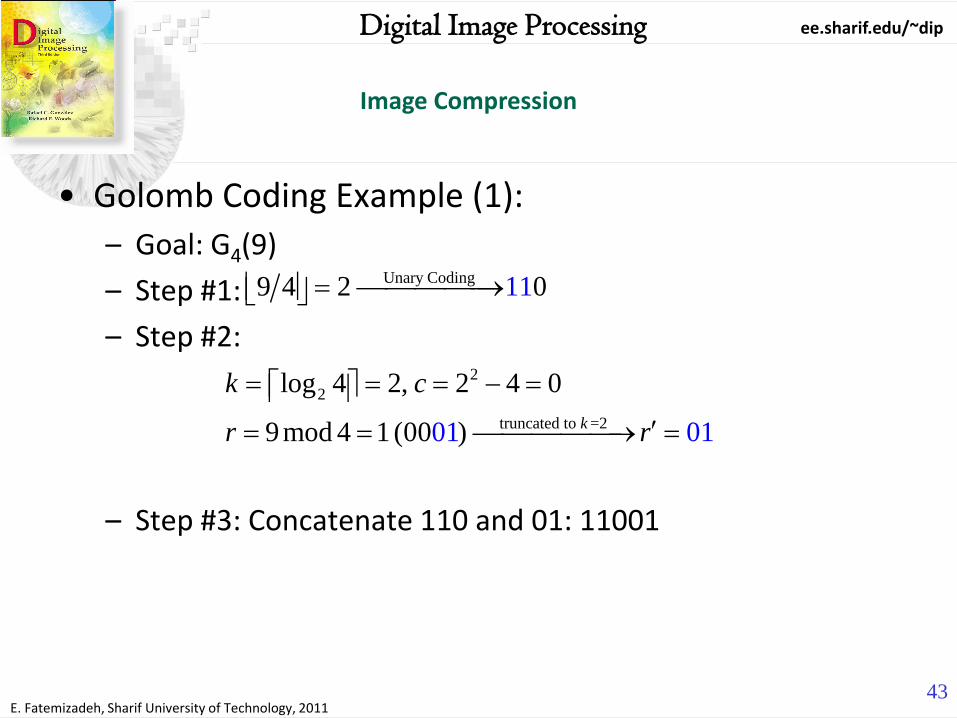
• Golomb Coding Example (1):
– Goal: G4(9)
– Step #1:
– Step #2:
– Step #3: Concatenate 110 and 01: 11001
Unary Coding9 4 0112
2
2
truncated to =2
log 4 2, 2 4 0
9mod 4 1(0 010 ) 01k
k c
r r

ee.sharif.edu/~dip
E. Fatemizadeh, Sharif University of Technology, 2011
44
Digital Image Processing
Image Compression
44
• Golomb Coding Example (2):
ee.sharif.edu/~dip
E. Fatemizadeh, Sharif University of Technology, 2011
45
Digital Image Processing
Image Compression
45
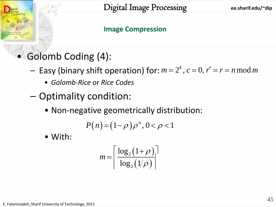
• Golomb Coding (4):
– Easy (binary shift operation) for: • Golomb-Rice or Rice Codes
– Optimality condition:
• Non-negative geometrically distribution:
• With:
2 , 0, modkm c r r n m
1 , 0 1nP n
2
2
log 1
log 1m

ee.sharif.edu/~dip
E. Fatemizadeh, Sharif University of Technology, 2011
46
Digital Image Processing
Image Compression
46
• Usability (1): – Intensity image distribution are NOT geometrical.
– Difference images are.
• How handle negative value: – Map to Odd and even non-negative integer:
2 0
2 1 0
n nM n
n n

ee.sharif.edu/~dip
E. Fatemizadeh, Sharif University of Technology, 2011
47
Digital Image Processing
Image Compression
47
• Usability (2):
– Geometrically distribution(s)
– Difference image histogram
– Mapped histogram

ee.sharif.edu/~dip
E. Fatemizadeh, Sharif University of Technology, 2011
48
Digital Image Processing
Image Compression
48
• Use Golomb Coding in image:
– Consider P(n-μ) instead of P(n), μ: mean intensity
– Map the negative image.
– Code using Gm(n)

ee.sharif.edu/~dip
E. Fatemizadeh, Sharif University of Technology, 2011
49
Digital Image Processing
Image Compression
49
• Golomb Image Coding Example (1):
Map
pin
g

ee.sharif.edu/~dip
E. Fatemizadeh, Sharif University of Technology, 2011
50
Digital Image Processing
Image Compression
50
• Golomb Image Coding Results (1):
– G1(n)
• C=4.5
• 88% of theoretical compression ratio (4.5/5.1)
• 96% of Huffman coding compression (Both in MATLAB) – Less computational efforts

ee.sharif.edu/~dip
E. Fatemizadeh, Sharif University of Technology, 2011
51
Digital Image Processing
Image Compression
51
• Golomb Image Coding Example (2):
– G1(n) • C=0.0922!!!
• Data Expansion
– Golomb is model based

ee.sharif.edu/~dip
E. Fatemizadeh, Sharif University of Technology, 2011
52
Digital Image Processing
Image Compression
52
• Golomb Exponential Coding of order k:
– Step #1: Find non-negative integer i such that:
• And form unary coding of i.
– Step #2: Truncate the following binary representation to k+I (LSB)
– Step #3: Concatenate results of step #1 and #2
– k=0 is known as Elias-gamma code
1
0 0
2 2i i
j k j k
j j
n
1
0
2i
j k
j
n

ee.sharif.edu/~dip
E. Fatemizadeh, Sharif University of Technology, 2011
53
Digital Image Processing
Image Compression
53
• Example:
– Let’d compute: • Step #1:
• Step #2:
• Step #3: 1110001
0
exp 8G
Unary Coding
20 log 9 3 1110k i
3 1Unary Coding Trunc. to 3+0
0
8 2 8 1 2 4 1 0 000 101j k
j

ee.sharif.edu/~dip
E. Fatemizadeh, Sharif University of Technology, 2011
54
Digital Image Processing
Image Compression
54
• Arithmetic Coding:
– Stream-based (A string of source symbols is encoded as a string of code symbols):
– Free of the integer number of bits/symbol restriction and more efficient.
– Arithmetic coding may reach the theoretical bound of coding efficiency specified in the noiseless source coding theorem for any information source.
– JBIG1, JBIG2, JPEG-2000, H264, MPEG-4 AVC

ee.sharif.edu/~dip
E. Fatemizadeh, Sharif University of Technology, 2011
55
Digital Image Processing
Image Compression
55
• Arithmetic Coding, Basic idea:
– With n bits, a code interval of [0,1] divided to 2n parts with
length of 2-n.
– Vise versa A=2-n can be coded using –log2A.
000 001 010 011 100 101 110 111
00 01 10 11
0 1
0 0.125 0.250 0.375 0.500 0.625 0.750 0.875 1

ee.sharif.edu/~dip
E. Fatemizadeh, Sharif University of Technology, 2011
56
Digital Image Processing
Image Compression
56
• Arithmetic Coding-Basic Idea:
– Represent the entire input stream as a small interval between the range [0,1].
– 1. Divide interval ([0,1]) to subintervals according to probability distribution.
– The first symbol interval is taken and again divide to sub interval with length of relative to probabilities.
– Now take second symbol interval and continue …

ee.sharif.edu/~dip
E. Fatemizadeh, Sharif University of Technology, 2011
57
Digital Image Processing
Image Compression
57
• Arithmetic Encoding By Example:
– Stream is baca
Si Pi Range
a 0.5 [0.0-0.5)
b 0.25 [0.5-0.75)
c 0.25 [0.75-1.0)
Range
[0.5-0.625)
[0.625-0.6875)
[0.6875-0.75)
Range
[0.5-0.5625)
[0.5625-0.59375)
[0.59375-0.625)
Range
[0.59375-0.609375)
[0.609375-0.6171875)
[0.6171875-0.625)

ee.sharif.edu/~dip
E. Fatemizadeh, Sharif University of Technology, 2011
58
Digital Image Processing
Image Compression
58
• Arithmetic Decoding By Example:
– Code is 0.59375
• 0.5<0.59375<0.75 b (b section of main interval)
• 0.5<0.59375<0.625 a (a section of subinterval b)
• 0.59375<0.59375<0.625 c (c section of subinterval a)
• 0.59375<0.59375<0.609375 a (a section of suninterval c)
– Loop. For all the symbols.
• Range = high_range of the symbol - low_range of the symbol
• Number = number - low_range of the symbol
• Number = number / range
• Stop for Number = 0

ee.sharif.edu/~dip
E. Fatemizadeh, Sharif University of Technology, 2011
59
Digital Image Processing
Image Compression
59
• Implementation:
– Change [0,1] to [0000H,FFFFH]
– Change Probabilities value

ee.sharif.edu/~dip
E. Fatemizadeh, Sharif University of Technology, 2011
60
Digital Image Processing
Image Compression
60
• Arithmetic Coding
ee.sharif.edu/~dip
E. Fatemizadeh, Sharif University of Technology, 2011
61
Digital Image Processing
Image Compression
61
• Lempel-Ziv-Welch (LZW) Coding
– Reduce Spatial-Coding redundancy
– Assign fixed-length codewords to variable-length sequences of source symbols.
– No priori knowledge about intensity probability
– GIF, TIFF, PNG, PDF

ee.sharif.edu/~dip
E. Fatemizadeh, Sharif University of Technology, 2011
62
Digital Image Processing
Image Compression
62
• Introductory Example:
• First Order Entropy:
21 21 21 95 169 243 243 243
21 21 21 95 169 243 243 243
21 21 21 95 169 243 243 243
21 21 21 95 169 243 243 243
Gray level Count Probability
21 12 0.375
95 4 0.125
169 4 0.125
243 12 0.375
1.81 bits/pixel

ee.sharif.edu/~dip
E. Fatemizadeh, Sharif University of Technology, 2011
63
Digital Image Processing
Image Compression
63
• Introductory Example: – Second Order Entropy:
1.25 bits/pixel
Gray level
pair Count Probability
(21, 21) 8 0.250
(21, 95) 4 0.125
(95, 169) 4 0.125
(169, 243) 4 0.125
(243, 243) 8 0.25
(243, 21) 4 0.125

ee.sharif.edu/~dip
E. Fatemizadeh, Sharif University of Technology, 2011
64
Digital Image Processing
Image Compression
64
• Meta AlgorithmWikipedia:
– Initialize the dictionary to contain all strings of length one.
– Find the longest string W in the dictionary that matches the current input.
– Emit the dictionary index for W to output and remove W from the input.
– Add W followed by the next symbol in the input to the dictionary.
– Go to Step 2.

ee.sharif.edu/~dip
E. Fatemizadeh, Sharif University of Technology, 2011
65
Digital Image Processing
Image Compression
65
• ExampleWikipedia:
– String to be code: TOBEORNOTTOBEORTOBEORNOT#
– 1) Initial Dictionary:
Symbol Code Symbol Code Symbol Code
# 0 I 9 R 18
A 1 J 10 S 19
B 2 K 11 U 20
C 3 L 12 V 21
D 4 M 13 W 22
E 5 N 14 X 23
F 6 O 15 Y 24
G 7 P 16 Z 25
H 8 Q 17 # 26

ee.sharif.edu/~dip
E. Fatemizadeh, Sharif University of Technology, 2011
66
Digital Image Processing
Image Compression
66
• Example: TOBEORNOTTOBEORTOBEORNOT# Input
Code Output Sequence
New Dictionary Entry
Full Conjecture
20 T 27: T?
15 O 27: TO 28: O?
2 B 28: OB 29: B?
5 E 29: BE 30: E?
15 O 30: EO 31: O?
18 R 31: OR 32: R?
14 N 32: RN 33: N?
15 O 33: NO 34: O?
20 T 34: OT 35: T?
27 TO 35: TT 36: TO?
29 BE 36: TOB 37: BE?
31 OR 37: BEO 38: OR?
36 TOB 38: ORT 39: TOB?
30 EO 39: TOBE 40: EO?
32 RN 40: EOR 41: RN?
34 OT 41: RNO 42: OT?
0 #
ee.sharif.edu/~dip
E. Fatemizadeh, Sharif University of Technology, 2011
67
Digital Image Processing
Image Compression
67
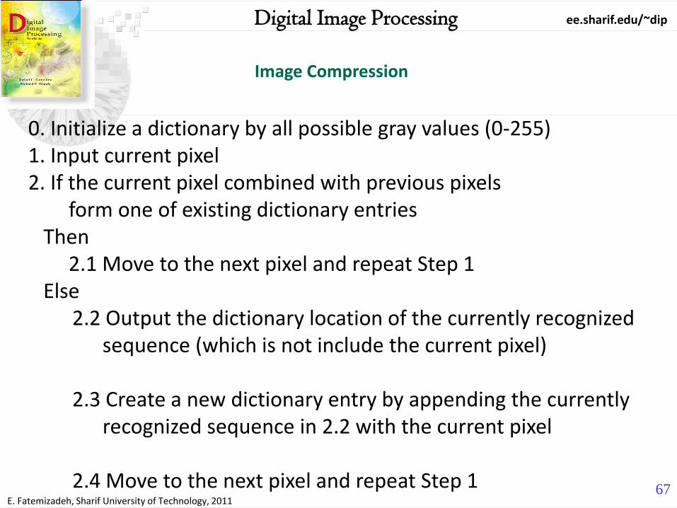
0. Initialize a dictionary by all possible gray values (0-255) 1. Input current pixel 2. If the current pixel combined with previous pixels form one of existing dictionary entries Then 2.1 Move to the next pixel and repeat Step 1 Else
2.2 Output the dictionary location of the currently recognized sequence (which is not include the current pixel) 2.3 Create a new dictionary entry by appending the currently recognized sequence in 2.2 with the current pixel 2.4 Move to the next pixel and repeat Step 1

ee.sharif.edu/~dip
E. Fatemizadeh, Sharif University of Technology, 2011
68
Digital Image Processing
Image Compression
68
• LZW for Image coding:
– Initialize a dictionary by all possible gray values (0-255)
– (1) Input current pixel
– (2) If the (current pixel concatenate previous pixels) exists in dictionary, then
• (2-1) Move to the next pixel and repeat Step 1
– Else • (2-2) Output the dictionary location of the currently recognized
sequence (which is not include the current pixel)
• (2-3) Create a new dictionary entry by appending the currently recognized sequence in (2-2) with the current pixel
• (2-4) Move to the next pixel and repeat Step 1

ee.sharif.edu/~dip
E. Fatemizadeh, Sharif University of Technology, 2011
69
Digital Image Processing
Image Compression
69
Input
39
39
126
126
39
39
126
126
39
39
126
126
Dictionary
0 0
1 1
… …
255 255
256 39-39
257 39-126
258 126-126
259 126-39
260 39-39-126
261 126-126-39
262 39-39-126-126
Encoded
Output (9 bits)
39
39
126
126
256
258
260
Sequences
39
39
126
126
39
39-39
126
126-126
39
39-39
39-39-126
126

ee.sharif.edu/~dip
E. Fatemizadeh, Sharif University of Technology, 2011
70
Digital Image Processing
Image Compression
70
• Binary image compression:
– A very simple approach: 8 pixels to one byte (code redundancy)
– Constant Area Coding (CAC):
• Image is divided to blocks (p×q): – White, Black, and Mixed
• Coding: – Most Probable (W/B/M) will code by one bit (0)
– Two others will code by two bits(10/11)
– Mixed code is prefix of its data

ee.sharif.edu/~dip
E. Fatemizadeh, Sharif University of Technology, 2011
71
Digital Image Processing
Image Compression
71
• Binary image compression:
– White Block Skipping (WBS):
• 0 for whole white blocks
• 1 is used as prefix for mixed or whole black (less probable)
– Symbol-based (Token-based) Coding:
• Image modeled as a collection of frequently occurred sub-images (symbols or tokens)
• (xi,yi,ti):(xi,yi) are position of symbols and ti position of symbol in dictionary
– JBIG2 (Text Halftone, Generic region), Page: 561-2

ee.sharif.edu/~dip
E. Fatemizadeh, Sharif University of Technology, 2011
72
Digital Image Processing
Image Compression
72
• Symbol-based (Token-based) Coding:
– Image modeled as a collection of frequently occurred sub-images (symbols or tokens)
– (xi,yi,ti):(xi,yi) are position of symbols and ti position of symbol in dictionary

ee.sharif.edu/~dip
E. Fatemizadeh, Sharif University of Technology, 2011
73
Digital Image Processing
Image Compression
73
• One dimensional Run Length Coding (RLE):
– Basic idea:
• Code each cluster of white (1) and Black (0) pixel by its length (Or cluster of constant gray level).
• Two Approach: – Specify value of first run of each row.
– Assume each row begin with white (its length may be zero)
– We may use variable length coding for each length of black or white.
– Facsimile (FAX) and BMP

ee.sharif.edu/~dip
E. Fatemizadeh, Sharif University of Technology, 2011
74
Digital Image Processing
Image Compression
74
• Run-Length Coding Implementation:
– One-dimensional CCITT
– Two-Dimensional CCITT • Coding Black-to-white and white-to-black transition
– Read pages 555-559
ee.sharif.edu/~dip
E. Fatemizadeh, Sharif University of Technology, 2011
75
Digital Image Processing
Image Compression
75
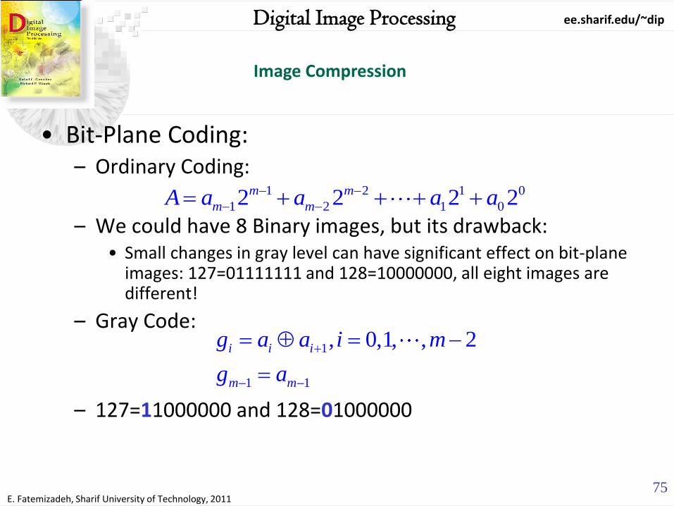
• Bit-Plane Coding: – Ordinary Coding:
– We could have 8 Binary images, but its drawback: • Small changes in gray level can have significant effect on bit-plane
images: 127=01111111 and 128=10000000, all eight images are different!
– Gray Code:
– 127=11000000 and 128=01000000
1 2 1 0
1 2 1 02 2 2 2m m
m mA a a a a
1
1 1
, 0,1, , 2i i i
m m
g a a i m
g a
ee.sharif.edu/~dip
E. Fatemizadeh, Sharif University of Technology, 2011
76
Digital Image Processing
Image Compression
76
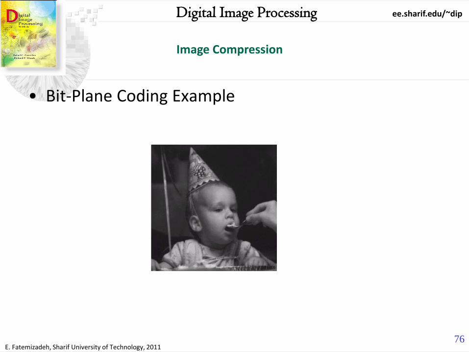
• Bit-Plane Coding Example

ee.sharif.edu/~dip
E. Fatemizadeh, Sharif University of Technology, 2011
77
Digital Image Processing
Image Compression
77
Gray Binary
Bit 7
Bit 6
Bit 5
Bit 4
Gray Images are less complex
• Example:
– Bit-Planes (7-4)

ee.sharif.edu/~dip
E. Fatemizadeh, Sharif University of Technology, 2011
78
Digital Image Processing
Image Compression
78
• Example:
– Bit-Planes (3-0)
Gray Binary
Bit 3
Bit 2
Bit 1
Bit 0
Gray Images are less complex

ee.sharif.edu/~dip
E. Fatemizadeh, Sharif University of Technology, 2011
79
Digital Image Processing
Image Compression
79
• JBIG2 Results:

ee.sharif.edu/~dip
E. Fatemizadeh, Sharif University of Technology, 2011
80
Digital Image Processing
Image Compression
80
• Block Transform Coding:
– A Reversible- Linear transform maps the image to a set of coefficients.
– These coefficients then quantized and coded. (Local/Global)

ee.sharif.edu/~dip
E. Fatemizadeh, Sharif University of Technology, 2011
81
Digital Image Processing
Image Compression
81
• Transform Selection:
– Compression is done during quantization NOT transforming.
– Type of transformation relate to Compression ratio.
– Separable Transform:
– Symmetric Transform:
1 1
0 0
1 1
0 0
, , , ; ,
, , , ; ,
n n
x y
n n
u v
T u v g x y r x y u v
g x y T u v s x y u v
1 2, ; , , ,r x y u v r x u r y v
1 1, ; , , ,r x y u v r x u r y v
ee.sharif.edu/~dip
E. Fatemizadeh, Sharif University of Technology, 2011
82
Digital Image Processing
Image Compression
82
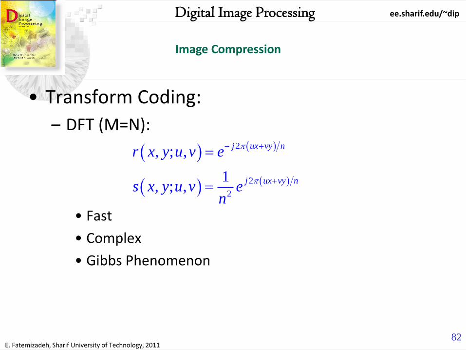
• Transform Coding:
– DFT (M=N):
• Fast
• Complex
• Gibbs Phenomenon
2
2
2
, ; ,
1, ; ,
j ux vy n
j ux vy n
r x y u v e
s x y u v en

ee.sharif.edu/~dip
E. Fatemizadeh, Sharif University of Technology, 2011
83
Digital Image Processing
Image Compression
83
• DFT Basis Function:
ee.sharif.edu/~dip
E. Fatemizadeh, Sharif University of Technology, 2011
84
Digital Image Processing
Image Compression
84
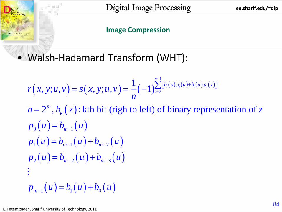
• Walsh-Hadamard Transform (WHT):
1
0
0 1
1 1 2
2 2 3
1 1 0
1, ; , , ; , 1
2 , : kth bit (righ to left) of binary representation of
m
i i i i
i
b x p u b u p v
m
k
m
m m
m m
m
r x y u v s x y u vn
n b z z
p u b u
p u b u b u
p u b u b u
p u b u b u

ee.sharif.edu/~dip
E. Fatemizadeh, Sharif University of Technology, 2011
85
Digital Image Processing
Image Compression
85
• Walsh-Hadamard Basis Function:

ee.sharif.edu/~dip
E. Fatemizadeh, Sharif University of Technology, 2011
86
Digital Image Processing
Image Compression
86
• Discrete Cosine Transform (DCT):
, ; , , ; ,
2 1 2 1cos cos
2 2
10
21,2, , 1
r x y u v s x y u v
x u y vu v
n n
un
u
u nn

ee.sharif.edu/~dip
E. Fatemizadeh, Sharif University of Technology, 2011
87
Digital Image Processing
Image Compression
87
• DCT Basis Function:

ee.sharif.edu/~dip
E. Fatemizadeh, Sharif University of Technology, 2011
88
Digital Image Processing
Image Compression
88
• Example:
– n=8,
– Truncating 50% of coefficients
DFT (2.32) WHT (1.78) DCT (1.13)

ee.sharif.edu/~dip
E. Fatemizadeh, Sharif University of Technology, 2011
89
Digital Image Processing
Image Compression
89
• Transform Coding Details:
– Consider a sub-image (block-wise processing):
1 1
0 0
1 1
0 0
, 1, 1
, 0,0
, , , ; ,
,
Matrix Formulation:
, ; ,
u v
uv
u v
i j n n
uv i j
g x y T u v s x y u v
T u v
s h i j u v
G S
S
n n
n n

ee.sharif.edu/~dip
E. Fatemizadeh, Sharif University of Technology, 2011
90
Digital Image Processing
Image Compression
90
• Transform Coding Details:
– Transform Masking Function:
1 1
0 0
0 , in a predefined region,
1 o.w.
ˆ , , Compressed Imageuv
u v
T u vu v
u v T u v
G Sn n

ee.sharif.edu/~dip
E. Fatemizadeh, Sharif University of Technology, 2011
91
Digital Image Processing
Image Compression
91
• Transform Coding Details:
– Error Analysis:
22
21 1 1 1
0 0 0 0
21 1
0 0
1 12
, 20 0
ˆ
, , ,
, 1 ,
Orthonormality of Transform Coeffs1 , :
N 0,
ms
uv uv
u v u v
uv
u v
T u vu v
e E
E T u v u v T u v
E T u v u v
u v
G G
S S
S
G
n n n n
n n
n n
ee.sharif.edu/~dip
E. Fatemizadeh, Sharif University of Technology, 2011
92
Digital Image Processing
Image Compression
92
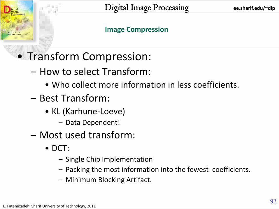
• Transform Compression: – How to select Transform:
• Who collect more information in less coefficients.
– Best Transform: • KL (Karhune-Loeve)
– Data Dependent!
– Most used transform: • DCT:
– Single Chip Implementation
– Packing the most information into the fewest coefficients.
– Minimum Blocking Artifact.

ee.sharif.edu/~dip
E. Fatemizadeh, Sharif University of Technology, 2011
93
Digital Image Processing
Image Compression
93
• Periodicity Implicit DFT and DCT
– Gibbs phenomenon causes erroneous boundary • Blocking artifacts
DFT
DCT

ee.sharif.edu/~dip
E. Fatemizadeh, Sharif University of Technology, 2011
94
Digital Image Processing
Image Compression
94
• Block size effect:
– Small Blocks: • Faster
• More blocking effect (correlation between neighboring pixels)
• Low compression ratio
– Large Block: • Slower
• Better compression in “flat” regions.
• Lower Blocking Effect
– Power of 2, for fast implementation.

ee.sharif.edu/~dip
E. Fatemizadeh, Sharif University of Technology, 2011
95
Digital Image Processing
Image Compression
95
• Block-Size and Transform Effects:

ee.sharif.edu/~dip
E. Fatemizadeh, Sharif University of Technology, 2011
96
Digital Image Processing
Image Compression
96
• Block Size effect for DCT:
– Reconstruct using 25% of the DCT coefficients
Original 2×2 4×4 8×8

ee.sharif.edu/~dip
E. Fatemizadeh, Sharif University of Technology, 2011
97
Digital Image Processing
Image Compression
97
• Bit Allocation:
– Bio Allocation: Truncation-Quantization-Coding
– How to select retained coefficients. • Maximum Magnitude (Threshold Coding)
• Maximum Variance (Zonal Coding)
– Threshold Coding: • Keeping P-largest coefficients.
– Zonal Coding: • DCT Coeffs. are considered as RV’s , all statistics computed using
ensemble of transformed subimages.
• Keeping P-largest variances (same -P (u,v)’s for all subimages.)

ee.sharif.edu/~dip
E. Fatemizadeh, Sharif University of Technology, 2011
98
Digital Image Processing
Image Compression
98
• Threshold vs. Zonal Coding:
– Keep coefficients 8 out of 64
RMS=4.5
RMS=6.5

ee.sharif.edu/~dip
E. Fatemizadeh, Sharif University of Technology, 2011
99
Digital Image Processing
Image Compression
99
• Zonal Coding Implementation:
– Ensemble average over MN/n2 subimages transforms and select non zero χ(u,v) , Zonal Masking. (High variances)
• 1 or 0 for each position in transform domain, Zonal Mask
• Number of bits used to code each coefficients, Zonal bit allocation
– Quantization of the retained coefficients: • Fixed Length (Uniformly Quantized)
• Optimal Quantizer:
– A model for DCT coefficients:
» Rayleigh for DC component. ( A positive RV’s)
» Laplacian or Gaussian for others (CLT theorem)

ee.sharif.edu/~dip
E. Fatemizadeh, Sharif University of Technology, 2011
100
Digital Image Processing
Image Compression
100
Z-Coding # of bits
• Zonal Coding Example:

ee.sharif.edu/~dip
E. Fatemizadeh, Sharif University of Technology, 2011
101
Digital Image Processing
Image Compression
101
• Threshold Coding Implementation:
– An Adaptive mask selection of non-zero χ(u,v)
– Location of maximum magnitude vary from one sub-image to another.
• Re-order 2D DCT to a 1D (Run Length Coded Sequence) in a zigzag arrangement.

ee.sharif.edu/~dip
E. Fatemizadeh, Sharif University of Technology, 2011
102
Digital Image Processing
Image Compression
102
• Why zigzag arrangement:
– This is done so that the coefficients are in order of increasing frequency.
– This improves the compression of run-length encoding.

ee.sharif.edu/~dip
E. Fatemizadeh, Sharif University of Technology, 2011
103
Digital Image Processing
Image Compression
103
T-Coding Zigzag tracing
• Threshold Coding Example:

ee.sharif.edu/~dip
E. Fatemizadeh, Sharif University of Technology, 2011
104
Digital Image Processing
Image Compression
104
• Thresholding:
– A single global threshold for all subimages.
• Different CR from image to image
– A different threshold for each subimages.
• N-Largest coding (same number of images are discarded)
• Same CR for all images.
– A variable threshold as a function of location.
• Different CR from image to image.
• Combined Quantization and Thresholding.

ee.sharif.edu/~dip
E. Fatemizadeh, Sharif University of Technology, 2011
105
Digital Image Processing
Image Compression
105
• Location Variant Thresholding:
,ˆ ,,
, : Elements of Transform Normalization
ˆ, , ,
:
,
:
inv
Compression
Decompression
T u vT u v round
Z u v
Z u v
T u v Z u v T u v f x y

ee.sharif.edu/~dip
E. Fatemizadeh, Sharif University of Technology, 2011
106
Digital Image Processing
Image Compression
106
Curve Normalization Matrix
,ˆ ,,
T u vT u v round
Z u v
ˆ , , ,2 2
,ˆ , 0, ,2
c cT u v k kc T u v kc
Z u vT u v T u v
• Thresholding-Quantization:
– Left for specific Z(u,v)=c
– Map of Z(u,v)

ee.sharif.edu/~dip
E. Fatemizadeh, Sharif University of Technology, 2011
107
Digital Image Processing
Image Compression
107
• Quantization Effect:
Z(u,v) 2Z(u,v) 4Z(u,v)
8Z(u,v) 16Z(u,v) 32Z(u,v)

ee.sharif.edu/~dip
E. Fatemizadeh, Sharif University of Technology, 2011
108
Digital Image Processing
Image Compression
108
• JPEG – Based on the Text Book
– Three different coding systems: • Lossy baseline coding system (most application)
• Greater Compression/Progressive reconstruction (Web)
• Lossles independent coding (reversible compression)

ee.sharif.edu/~dip
E. Fatemizadeh, Sharif University of Technology, 2011
109
Digital Image Processing
Image Compression
109
• Baseline system (Sequential baseline system):
– Input and Output precision: 8 bits
– Quantized DCT coefficients precision: 11 bits
– Performs in three steps: DCT, Quantization, VL coding
• Preprocessing:
– Level shifting (2k-1, k bit depth)
• Coding:
– Different VLS coding for nonzero AC and DC components.

ee.sharif.edu/~dip
E. Fatemizadeh, Sharif University of Technology, 2011
110
Digital Image Processing
Image Compression
110
• Sample subimages (8*8)

ee.sharif.edu/~dip
E. Fatemizadeh, Sharif University of Technology, 2011
111
Digital Image Processing
Image Compression
111
• Level shifting (-128)

ee.sharif.edu/~dip
E. Fatemizadeh, Sharif University of Technology, 2011
112
Digital Image Processing
Image Compression
112
• Forward DCT Transoform:
ee.sharif.edu/~dip
E. Fatemizadeh, Sharif University of Technology, 2011
113
Digital Image Processing
Image Compression
113
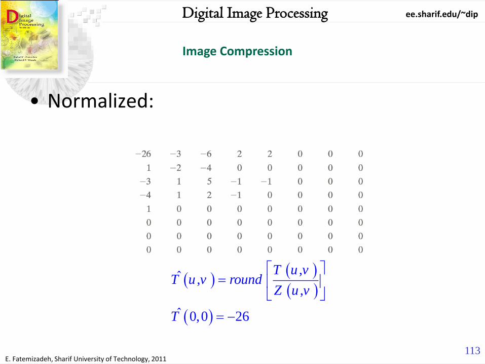
• Normalized:
,ˆ ,,
ˆ 0,0 26
T u vT u v round
Z u v
T

ee.sharif.edu/~dip
E. Fatemizadeh, Sharif University of Technology, 2011
114
Digital Image Processing
Image Compression
114
• Zig-Zag Scanning:
• Two different Coding for DC and AC
– See Tables A-3, A-4, A-5 for codebook

ee.sharif.edu/~dip
E. Fatemizadeh, Sharif University of Technology, 2011
115
Digital Image Processing
Image Compression
115
• Quantized Coefficients:

ee.sharif.edu/~dip
E. Fatemizadeh, Sharif University of Technology, 2011
116
Digital Image Processing
Image Compression
116
• Denormalization:
ˆ, , ,
0,0 416
0,0 415
T u v Z u v T u v
T
T

ee.sharif.edu/~dip
E. Fatemizadeh, Sharif University of Technology, 2011
117
Digital Image Processing
Image Compression
117
• Inverse DCT Transform:

ee.sharif.edu/~dip
E. Fatemizadeh, Sharif University of Technology, 2011
118
Digital Image Processing
Image Compression
118
• Level Shifting (+128):

ee.sharif.edu/~dip
E. Fatemizadeh, Sharif University of Technology, 2011
119
Digital Image Processing
Image Compression
119
• Difference Image:

ee.sharif.edu/~dip
E. Fatemizadeh, Sharif University of Technology, 2011
120
Digital Image Processing
Image Compression
120
• Example:
1:25
1:52

ee.sharif.edu/~dip
E. Fatemizadeh, Sharif University of Technology, 2011
121
Digital Image Processing
Image Compression
121
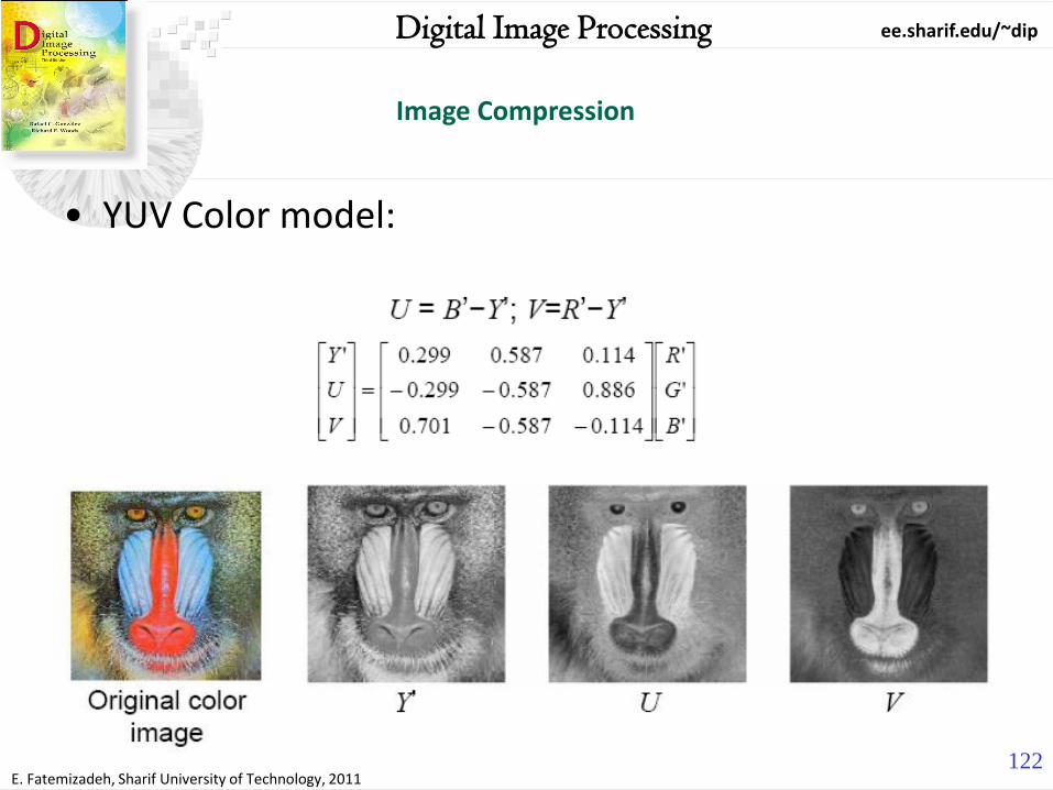
• JPEG (Joint Photographic Expert Group)
– Color Models
– Image Subsampling
– Coding (DC and AC)
ee.sharif.edu/~dip
E. Fatemizadeh, Sharif University of Technology, 2011
122
Digital Image Processing
Image Compression
122
• YUV Color model:

ee.sharif.edu/~dip
E. Fatemizadeh, Sharif University of Technology, 2011
123
Digital Image Processing
Image Compression
123
• YIQ Color Model:

ee.sharif.edu/~dip
E. Fatemizadeh, Sharif University of Technology, 2011
124
Digital Image Processing
Image Compression
124
• Chromatic components subsampling:

ee.sharif.edu/~dip
E. Fatemizadeh, Sharif University of Technology, 2011
125
Digital Image Processing
Image Compression
125
• Chrominance Decimation of eye:

ee.sharif.edu/~dip
E. Fatemizadeh, Sharif University of Technology, 2011
126
Digital Image Processing
Image Compression
126
• Compression Block Diagram

ee.sharif.edu/~dip
E. Fatemizadeh, Sharif University of Technology, 2011
127
Digital Image Processing
Image Compression
127
• Decompression Block Diagram

ee.sharif.edu/~dip
E. Fatemizadeh, Sharif University of Technology, 2011
128
Digital Image Processing
Image Compression
128
• DCT on Image block
– Each image is divided into 8×8 blocks. The 2D DCT is applied to each block image f(i, j), with output being the DCT coefficients F(u,v) for each block.

ee.sharif.edu/~dip
E. Fatemizadeh, Sharif University of Technology, 2011
129
Digital Image Processing
Image Compression
129
• Quantization:
– F(u,v) represents a DCT coefficient, Q(u,v) is a “quantization matrix” entry, and F(u,v) represents the quantized DCT coefficients which JPEG will use in the succeeding entropy coding.
• The quantization step is the main source for loss in JPEG compression.
• The entries of Q(u,v) tend to have larger values towards the lower right corner. This aims to introduce more loss at the higher spatial frequencies

ee.sharif.edu/~dip
E. Fatemizadeh, Sharif University of Technology, 2011
130
Digital Image Processing
Image Compression
130
• Quantization Table:
– Default Q(u,v) values obtained from psychophysical studies with the goal of maximizing the compression ratio while minimizing perceptual losses in JPEG images.

ee.sharif.edu/~dip
E. Fatemizadeh, Sharif University of Technology, 2011
131
Digital Image Processing
Image Compression
131
• DCT + Quantization:
Encoder
Decoder

ee.sharif.edu/~dip
E. Fatemizadeh, Sharif University of Technology, 2011
132
Digital Image Processing
Image Compression
132
• DPCM: Differential Pulse Code Modulation
– Used for DC components compression: • DC coefficient is unlikely to change drastically within a short
distance so we expect DPCM codes to have small magnitude and variance.
– Entropy coding of DC components: • Huffman
150 155 149 152 144 150 5 6 3 8

ee.sharif.edu/~dip
E. Fatemizadeh, Sharif University of Technology, 2011
133
Digital Image Processing
Image Compression
133
• RLC: Run Length Coding – Used for AC components compression:
• RLC is effective if the information source has the property that symbols tend to form continuous groups. In this case, the quantized DCT coefficients tend to form continuous groups of 0s.
– Used in Conjunction with zig-zag scan
– Entropy coding of DC components: • Huffman

ee.sharif.edu/~dip
E. Fatemizadeh, Sharif University of Technology, 2011
134
Digital Image Processing
Image Compression
134
• RLC: Run Length Coding

ee.sharif.edu/~dip
E. Fatemizadeh, Sharif University of Technology, 2011
135
Digital Image Processing
Image Compression
135
• Lossless Predictive Coding:
– Code only new information in each pixel.
– New Information: Difference between two successive pixel.
– en is coded with a variable-length coding (symbol Encoder)
: New incoming pixel value.
ˆ : Prediction of based on a limited range history
n
n n
f
f f
ˆn n ne f f

ee.sharif.edu/~dip
E. Fatemizadeh, Sharif University of Technology, 2011
136
Digital Image Processing
Image Compression
136
• Prediction:
– An optimal (local/global) and adaptive predictor:
– A nearest integer operator is needed
1-D
1 1
ˆ ˆ , ,m m
n i i
i i
f round f n i f x y round f x y i

ee.sharif.edu/~dip
E. Fatemizadeh, Sharif University of Technology, 2011
137
Digital Image Processing
Image Compression
137
• Coder and Decoder:

ee.sharif.edu/~dip
E. Fatemizadeh, Sharif University of Technology, 2011
138
Digital Image Processing
Image Compression
138
• Lossless Predictive Coding:
– For 2D images:
– Example:
• Zero difference is code with 128
• Negative/Positive error are coded with dark light region.
ˆ , ,m m
i
i m j m
f x y round f x i y j
ˆ , 1nf round f x y

ee.sharif.edu/~dip
E. Fatemizadeh, Sharif University of Technology, 2011
139
Digital Image Processing
Image Compression
139
• Example:
– Prediction residual
– α=1
– CR = 8/3.99 = 2
– Residual PDF
ˆ, , ,e x y f x y f x y
2
1
2
e
e
e
e
P e e

ee.sharif.edu/~dip
E. Fatemizadeh, Sharif University of Technology, 2011
140
Digital Image Processing
Image Compression
140
• Example (Temporal Redundancy):
ˆ , , , , 1 , 1
ˆ, , , , , , 1
f x y t round f x y t
e x y t f x y t f x y t

ee.sharif.edu/~dip
E. Fatemizadeh, Sharif University of Technology, 2011
141
Digital Image Processing
Image Compression
141
• Motion Compensated Prediction Residuals
– Self study (589-596)

ee.sharif.edu/~dip
E. Fatemizadeh, Sharif University of Technology, 2011
142
Digital Image Processing
Image Compression
142
• Lossy Compression:
– JPEG, JPEG2000, GIF
– 1:10 to 1:50

ee.sharif.edu/~dip
E. Fatemizadeh, Sharif University of Technology, 2011
143
Digital Image Processing
Image Compression
143
• Lossy Predictive Coding:
– Map prediction error into a limited range of outputs (control compression ratio)
ˆn n nf e f

ee.sharif.edu/~dip
E. Fatemizadeh, Sharif University of Technology, 2011
144
Digital Image Processing
Image Compression
144
• Delta Modulation:
1ˆ 1
0
O.W.
Singel bit code (1bit/pixel)
n n
n
n
f f
ee

ee.sharif.edu/~dip
E. Fatemizadeh, Sharif University of Technology, 2011
145
Digital Image Processing
Image Compression
145
• Optimal Prediction:
22
1
2
2
1
, 1
2 2
11
ˆ ˆ ˆ,
ˆ
: Image Autocorrelation Matrix, ,
n n n n n n n n n
m
n i n i
i
m
n n i n i
i
m
n i n j i j
mm
n n k e i n n iki
E e E f f f e f e f f
f f
E e E f f
i j E f f
k E f f E f f
-1α = R r
R R
r

ee.sharif.edu/~dip
E. Fatemizadeh, Sharif University of Technology, 2011
146
Digital Image Processing
Image Compression
146
• Optimal Prediction:
– Computation for image by image is hard.
– Global coefficient is computed by assuming a simple image model.
2
1 2 3 4
1 2 3 4
m
i
i=1
, ,
ˆ , , 1 1, 1 1, 1, 1
, , , 0
and : Horizontal and Vertical correlation coefficient
Dynamic Range Const.: 1
i j
v h
h h v v
h v
E f x y f x i y i
f x y f x y f x y f x y f x y
ee.sharif.edu/~dip
E. Fatemizadeh, Sharif University of Technology, 2011
147
Digital Image Processing
Image Compression
147
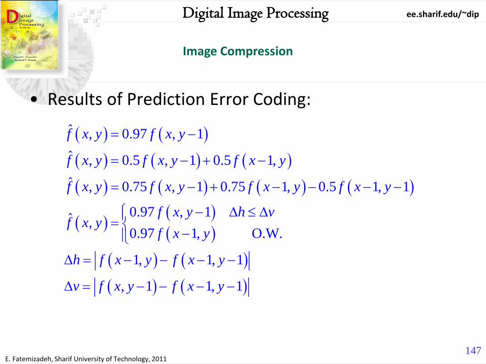
• Results of Prediction Error Coding:
ˆ , 0.97 , 1
ˆ , 0.5 , 1 0.5 1,
ˆ , 0.75 , 1 0.75 1, 0.5 1, 1
0.97 , 1ˆ ,0.97 1, O.W.
1, 1, 1
, 1 1, 1
f x y f x y
f x y f x y f x y
f x y f x y f x y f x y
f x y h vf x y
f x y
h f x y f x y
v f x y f x y

ee.sharif.edu/~dip
E. Fatemizadeh, Sharif University of Technology, 2011
148
Digital Image Processing
Image Compression
148
• Example:
– Prediction Errors
rms = 11.1 rms = 9.8
rms = 9.1 rms = 9.7

ee.sharif.edu/~dip
E. Fatemizadeh, Sharif University of Technology, 2011
149
Digital Image Processing
Image Compression
149
• Optimal Quantizer:
– t=q(s)
– q(s)=-q(-s)
– Map s in (si,si+1] to ti
– What is best si and ti

ee.sharif.edu/~dip
E. Fatemizadeh, Sharif University of Technology, 2011
150
Digital Image Processing
Image Compression
150
• Lloyd-Max Quantizer
– For even p(s), E{(si-ti)2}will minimize with these
conditions:
1
, 1, 2, ,2
0 0
11, 2, , 1
2 2
2
,
i
i
s
i
s
ii
i i i i
Ls t p s ds i
i
t ti Ls i
Li
s s t t

ee.sharif.edu/~dip
E. Fatemizadeh, Sharif University of Technology, 2011
151
Digital Image Processing
Image Compression
151
• Lloyd-Max Quantizer
– L=2, 4, 8
– Laplacian pdf (σ=1)
– ti-ti-1= si-si-1=θ

ee.sharif.edu/~dip
E. Fatemizadeh, Sharif University of Technology, 2011
152
Digital Image Processing
Image Compression
152
• Wavelet Coding

ee.sharif.edu/~dip
E. Fatemizadeh, Sharif University of Technology, 2011
153
Digital Image Processing
Image Compression
153
• Wavelet Selection: Haar Daubechies
Symlet Cohen

ee.sharif.edu/~dip
E. Fatemizadeh, Sharif University of Technology, 2011
154
Digital Image Processing
Image Compression
154
• Wavelet Selection:
– Truncating the transforms below 1.5:

ee.sharif.edu/~dip
E. Fatemizadeh, Sharif University of Technology, 2011
155
Digital Image Processing
Image Compression
155
• Decomposition Level Selection:
– More scales More computational efforts
– An Experiments:
• Biorthogonal wavelet;
• Fixed global threshold (25);
• Truncate only details

ee.sharif.edu/~dip
E. Fatemizadeh, Sharif University of Technology, 2011
156
Digital Image Processing
Image Compression
156
• Jpeg 2000 (607-614)
– DC Level shift
– Convert using color video transform (RGB YCbCr)
– Convert the whole image to tile components
– Using different filter for lossy or loss-free compression
– Quantized the coefficients
– Arithmetic Coding

ee.sharif.edu/~dip
E. Fatemizadeh, Sharif University of Technology, 2011
157
Digital Image Processing
Image Compression
157
• Example:
– C=25, 52, 75, 105.

ee.sharif.edu/~dip
E. Fatemizadeh, Sharif University of Technology, 2011
158
Digital Image Processing
Image Compression
158
• Image Watermarking
– Skipped

ee.sharif.edu/~dip
E. Fatemizadeh, Sharif University of Technology, 2011
159
Digital Image Processing
Image Compression
159
• Matlab Command
– Huffmandeco, huffmandict, huffmanenco
– Arithdeco, arithenco
– Dpcmdeco, dpcmenco
– Lloyds, quantiz
– wcompress (wavelet image compression)