CFDLaboratory

“Four Decades of Weak Form CFD”

A. J. Baker, PhD, PE Professor Emeritus

The Computational Engineering Sciences UT Academic Program

Graduate education (1978 – 2007):16 (+ 2) PhD, 17 MSc degree completions70 archival journal articles138 conference proceedings3 (+ 1) textbooks, 9 monograph chapters4 Internet - enabled graduate courses

CFD Laboratory Track Record

Professional service:academic outreachGraduate CFD Certificatecommercial industry interaction

Funded research projects (1975 – 2010):DOD, NSF, DOE, FAA, NIOSH, . . ~ $7.3 (+ 1) M70 research contract reports

Academic Internet Outreach

Internet archived online courses:• Finite Element Analysis• Computational Engineering Sciences• Computational Fluid-Thermal Sciences• Advanced Topics in Turbulence

Towards: optimal modified continuous Galerkin CFDJ. Numerical Methods Fluids or Engineering:

Sahu(2007) “A modified conservation principles theory for an optimal Galerkin CFD algorithm”Wong(2002) “A 3-D incompressible Navier-Stokes velocity-vorticity weak form finite element algorithm”Chaffin(1995) “On Taylor weak statement finite element methods for CFD”Iannelli(1992) “A nonlinearly stable implicit FE algorithm for hypersonic aerodynamics”Baker(1973) “Finite element solution algorithm for viscous incompressible fluid dynamics”

J. Computer Methods Applied Mechanics & Engineering:Kim(1987) “A Taylor weak statement algorithm for hyperbolic conservations laws”Baker +(1984) “Review: a FE penalty parabolic Navier-Stokes algorithm for turbulent 3-D flows” Soliman(1981) “Accuracy and convergence of an FE algorithm for turbulent boundary layer flow”Baker +(1974) “Finite element solution theory for 3-D boundary region flows”

J. Computational Physics:Grubert(2010?) “A diagnostic analytic LES weak form CFD algorithm”Kolesnikov(2001) “An efficient high order Taylor weak statement for the Navier-Stokes equations”Soliman(1979) “Utility of a finite element algorithm for initial-value problems”Baker +(1976) “An implicit finite element algorithm for the boundary layer equations”

J. Numerical Heat Transfer: Part B, Fundamentals:Roy(1998) “A nonlinear subgrid-embedded FE basis for steady monotone CFD solutions”Williams(1996) “Incompressible CFD and the continuity constraint method for the 3-D Navier-Stokes equations”

CFD Lab Pivotal Research Pubs.

COMCO contributions: Paul Manhardt & Joe Orzechowski

1983 1991 2006

CFD Lab: Research ⇒ Academics

2010 (underway)

CFD Lab: Research ⇒ Academics

CONTENTS1 INTRODUCTION 2 CONCEPTS, TERMINOLOGY, METHODOLOGY3 AERODYNAMICS: potential flow,

GWSh theory exposition,transonic shock capturing

4 AERODYNAMICS: boundary layers, turbulence closure modeling, parabolic Navier-Stokes

5 THE NAVIER-STOKES EQUATIONS: theoretical fundamentals, constraints,spectral analyses, optimal GWSh + θTS

6 VECTOR FIELD THEORY IMPLEMENTATIONS:vorticity, streamfunction, velocity

7 PHYSICAL VARIABLES IMPLEMENTATIONS:NS and RaNS optimal weak forms

8 LARGE EDDY SIMULATION IMPLEMENTATIONS:SGS tensor, legacy modeling, rational LES,

optimal diagnostic analytic LES

APPENDIX: hypersonic aerodynamics PNS weak form algorithm

Fluid Dynamics in the FleshNavier-Stokes PDEs valid ∀ Re !

Re < 1000, single scale laminar Re > 5000, multi-scale “turbulent”

Turbulent flow generates too much information ⇒ filter it !

Can discrete CFD be truly predictive ∀ Re ? !

time-averaged⇐

left over⇒

NS PDE Filtering ⇔ Turbulent CFD

time-averaged state variable dynamics lost by averaging RaNS PDEs closure issues

generates 1 stress tensoreddy viscosity, νt, k-ε, k-ωlow Ret wall modelsdissipation is modeledRet stress tensor transport

numerical diffusion always non-uniform, unstructured mesh

non-conforming steady solutions compute fast !!

~ E08 node meshes

space filtered state variable dynamics retained in filtering LES PDEs closure issues

generates 4 stress tensorsconvection not resolved scalecross-stress tensor pairunresolved scale dissipation

SFS tensornumerical diffusion never

dense mesh for energy resolutionfilter measure δ ≥ 2h

time accurate unsteady solutions compute intensive !!

RaNS LES

Navier-Stokes Conservation Principles

( ) 00u jx j

ρ∂

= =∂

L

( ) 1 €g 02Re

u ui iu Pi ij it x xju uj i

jδ

∂ ∂ ∂ = + + − + Θ =∂ ∂ ∂

GrRe

L

( ) Ec1 0ReRe

u jt x xj j

∂Θ ∂ ∂Θ Θ = + Θ − − Φ =∂ ∂ ∂ Pr

L

( ) 1 0Re

Y YY u Y sjt x xj j

∂ ∂ ∂α α = + − − =α α α∂ ∂ ∂ ScL

DM:

DP:

DE:

DMα:

α

Flowfields parameterized by Re, Gr, Pr, Sc

Time-averaging NS PDEs ⇒ RaNS

State variable resolution:

NS convection term time-average:

Deviatoric eddy viscosity closure model:

( ) ( ) ( ), , , , j j ju t u u t Y Y Y′ ′ ′≡ + Θ ⇒ Θ + Θ ⇒ +x x x

) / 3j i j j i i j k k i jiD

j i u u u u u uu u ′ ′= + ≡ + τ + (τ δ

2i jD

i jt Sυτ ≡ −

1

2i jji

j i

uu

x xS

∂∂≡ +

∂ ∂

, .j j ju u u etc′ ′Θ = Θ + Θ

2 / , , . . . , Pr , Sct tt C k k withµυ ≡ ε ω

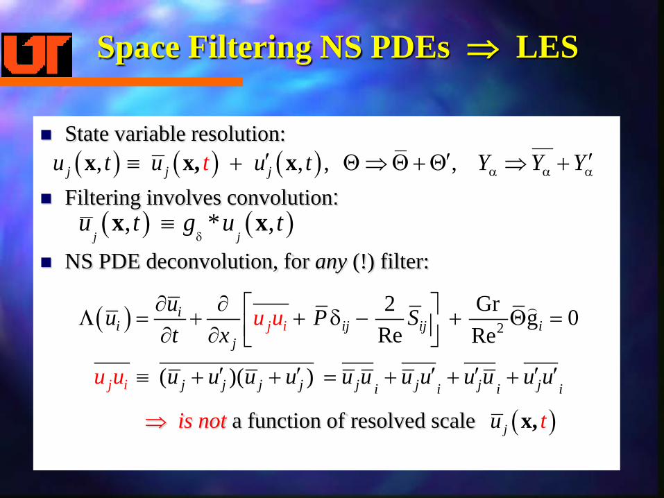
Space Filtering NS PDEs ⇒ LES

State variable resolution:

Filtering involves convolution:

NS PDE deconvolution, for any (!) filter:

⇒ is not a function of resolved scale

( ) 22 Gr g 0

Re Re

( )( )

ii ij ij i

j

j j j j j j j ji i i i

j i

j i

uu P St x

u u u u u u u u u uu u u

u u

u

∂ ∂ = + + δ − + Θ = ∂ ∂

′ ′ ′ ′ ′ ′≡ + + = + + +

L

( ) ( ) ( ), , , , j j ju t u u t Y Yt Yα α α′ ′ ′≡ + Θ ⇒ Θ + Θ ⇒ +x x, x

( ) ( ), * ,j j

u t g u tδ

≡x x

( )ju tx,

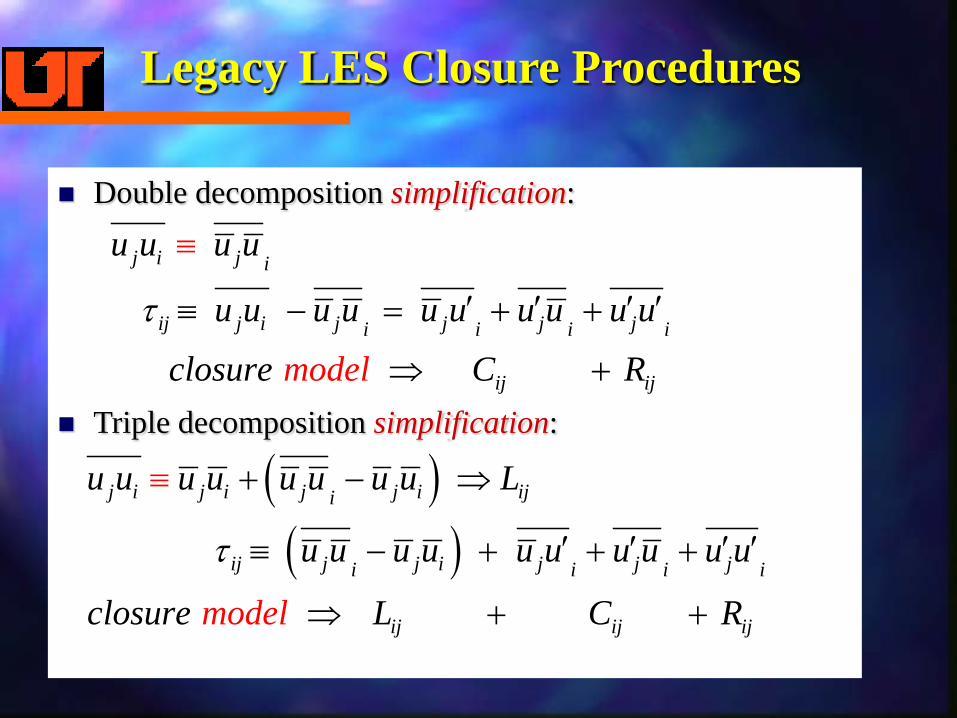
Legacy LES Closure Procedures

Double decomposition simplification:

Triple decomposition simplification:

( )( )

j i j i j j i iji

ij j j i j j ji i i i

ij ij ij

u u u u u u u u L

u u u u u u u u u u

closure L Cmodel R

τ

+ − ⇒

′ ′ ′ ′≡ − + + +

⇒ + +

≡

j i j i

ij j i j j j ji i i i

ij ij

u u u u

u u u u u u u u u u

closur modele C R

τ ′ ′ ′ ′≡ − = + +

⇒ +

≡

Legacy LES Eddy Viscosity Closure

Legacy LES and RaNS PDEs are identical ! !

Subgrid scale (SGS) tensor model requirement:

Deviatoric eddy viscosity model, normal stress ⇒ pressure:

( )SC ,i j i ji j i j

i j i j i j

C Rf f t S S

L Ci Rjτ 2+ ≅ ⇒ ( ), , ( ) + +

δ

x, u

2S

13 2 , Ci j i j k k i j i j i j i

D Dj

t tS Sτ τ + τ δ ⇒ τ − υ≡ δυ =≡

( ) 22 Gr g 0

Re Rej ii

i

jij i j ii j

uu u u P S

t xτ

∂ ∂ = + + δ − + + Θ = ∂ ∂ L

Rational LES Wavenumber Asymptotics

Gaussian filter: ( ) ( ) ( )/ 2 22 2, , exp / 2/n

g δ γ = γ π δ −γ δ δ x x

Polynomial approximations in wavenumber space

O(δ2) rational Pade′O(δ2) Taylor series O(δ4) rational Pade′

Convolution Exact in Rational LES

Space filtered convection nonlinearity, any filter:

Filter via convolution: Rational LES enables Fourier transforms:

j j j ji ii ij iu u u u u u u u u u′ ′ ′ ′= + + +

( ) ( ) ( ), , , ,i iu t g u tδ≡ δ γ ∗x x x

( ) ( ) ( )

( ) ( ) ( )

( ) ( ) ( ) ( ) ( )

( ) ( ) ( ) ( ) ( )

1 1 ,

1 1

1 1

j j ii

i i i i i

j j ii

j j ii

F u u F g F u u

F u F u fro mu u uF g

F u u F g F u F uF g

F u u F g F u F uF g

δ

δ

δδ

δδ

=

′ ′= − ≡ +

′ = ∗ −

′ = − ∗

Rational LES Deconvolution

O(δ2) Taylor series:

O(δ2) rational Pade′:

O(δ4) rational Pade′:

( )2 42

1

4j i

j j i j j ii il l

u uu u u u u u u u I Ox x

2 2 ∂ δ δ ∂′ ′+ + ⇒ + − ∇ + δ γ γ ∂ ∂

−

( )2

j ij j j j ii i

l li

u uu u u u u u u u Ox x

2 ∂ ∂δ 4′ ′+ + ⇒ + + δ γ ∂ ∂

( )

4

22 2

2 4 32

. .16

1j j j j ii i i

j ji i

j i

l l k k

u u u u u u u u I

u uu uu u Ox x x x

2 2 42

2

4

2

δ δ δ′ ′+ + ⇒ + − ∇ + ∇ × γ γ γ ∂ ∂ ∂ δ ∂∇ 6− ∇ ∇ + + δ ∂ ∂ ∂ ∂

−

γ

O( δ4) rLES Cross-Stress Tensor Pair

rLES deconvolution precisely extracts to O(δ2)

Clearing inverse ⇒ cross-stress tensor pair harmonic PDEs

DE, DMα cross-vector pair harmonic PDEs ⇒ NO Prt, Sct !

22

4 2u uC Cx x

∂ γ ∂− ∇ + = δ ∂ ∂

j ii j i j

l l

22

4 2 jj j

l l

uC C

x xΘ Θ ∂ γ ∂Θ

− ∇ + = δ ∂ ∂

22

4 2 jY Yj j

l l

u YC Cx x

α∂ γ ∂− ∇ + = δ ∂ ∂

2

1

2 4

u uC I

x x

2 2 ∂ ∂δ δ− ∇

γ γ≡

∂

−

∂

j ii j

l l

j i i ju u C+

Analytic rLES O(δ4) PDE System

rLES transport PDEs

rLES Poisson PDEs

definitions

( ) ( )vj j

jt x∂ ∂

= + − − =∂ ∂qq f f s 0L

( ) ( )2 , , 0P P P Ps −2= − ∇ − =δq q q qL

( ) ( )

2Re

1, , Re Pr

1 'ReSc

S u uij ju u P ij i ijui vu uj jj j

Cij

x jY

u Yj Y u Yj

C jYC j

x j

αα α α

′ ′− + δ + ∂Θ ′ ′≡ Θ = Θ + = − Θ

∂ + ∂ ′− ∂

Θ

q qq f f

2 €, , Gr / Re g , Ec/ Re, , , ( ) P PT TP YC C Cij j j si

Θ= φ = Θ Φ δq s

O(δ4) rLES Theory SFS Tensor rLES sub-filter scale (SFS) tensor is negligible !!

mimic NS viscous dissipation at unresolved scale threshold λ⇒ λ ~ δ ≥ 2h

RaNS experience: λ scale energy is O(2h) dispersion error !

⇒ via dispersion errorannihilation!

12 2 2 ( )

16 4j i j iu u I u u O

−26

2

δ ′ ′ = − ∇ ∇ ∇ + δ γ γ

4δ

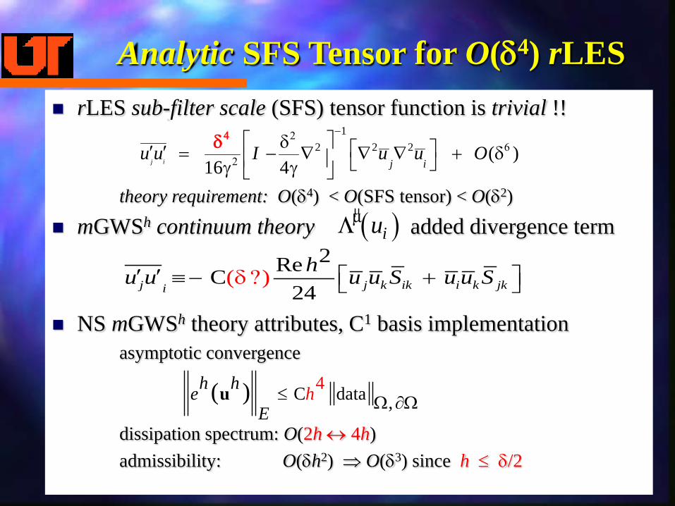
Analytic SFS Tensor for O(δ4) rLES rLES sub-filter scale (SFS) tensor function is trivial !!

theory requirement: O(δ4) < O(SFS tensor) < O(δ2)

mGWSh continuum theory added divergence term

NS mGWSh theory attributes, C1 basis implementationasymptotic convergence

dissipation spectrum: O(2h ↔ 4h)admissibility: O(δh2) ⇒ O(δ3) since h ≤ δ/2

C dat4 a ,( ) hh heE

≤ Ω ∂Ωu

2ReC24

( )j j k ik i k jki

hu u u u S u u Sδ ′ ′ ≡ − ? +

12 2 2 ( )

16 4j i j iu u I u u O

−26

2

δ ′ ′ = − ∇ ∇ ∇ + δ γ γ

4δ

( )iummL

Analytic Diagnostic rLES Closure

analytic diagnostic rLES transport PDE system

Dissipative flux vector, NS viscous + SFS terms, C ~ O(1)

( )2

2 C ReRe 24

1 C Re PrRe Pr 12

1 C Re ScRe S

2

2

2

2

c 1

S u u S u u Sij j k ik i k jk

v u uk jj x x

h

hh

h

j k

Y Yu uk jx xj kα α

+ + ∂Θ ∂Θ

= + ∂ ∂

∂ ∂

+

δ

δδ,

δ∂ ∂

q,f

( ) ( )( ) ( )vj j

jt xδ

∂ ∂= + − − =

∂ ∂δ

qq f f s 0L

optimal Modified Continuous Galerkin

analytic diagnostic state variable continuum approximation:

modified continuous Galerkin weak form extrema:

( ) ( ) ( ) ( ) 1

, ,N

Ni i ix t x t diag x t

β =β

≈ ≡ Ψ

∑q q Q

( ) ( ) ( ) ( ) 1

, ,N

NP i P i i Px t x t diag x tβ

β =

≈ ≡ Ψ

∑q q Q

( ) ( )GWS( ) d , 1mN Nim x for NτβΩ

≡ Ψ = ≤ β ≤∫q q 0mL

( ) ( )GWS( ) d 0, 1mN NP i Pm x for NτβΩ

≡ Ψ = ≤ β ≤∫q qm

mL

mGWSh O(h4, κh3, ∆t2) PDE System

optimal mGWSh transport mPDE:

optimal mGWSh Poisson mPDE:

for:

( ) ( )M[ ]m m m vj j

jt x∂ ∂

= + − − =∂ ∂qq f f s 0mL

( ) ( ) ( )22 21 , ,/12 0mP P P Ph s∇= − ∇ − + δ =q q q qmL

( ) ( )

11 2Re

11 , Re Pr

11ReS

2 2Re6 6

2 2Re Pr6 6

2 2R6c

eSc6

u u P C S u uj i ij ij ij j i

mv

h h

m u C uj jj

t t

j j x j

Yu Y Cj j

h ht t

h ht tα

′ ′+ + δ + + −

∂ΘΘ ′ ′= + Θ + = + − Θ ∂

+ + +

∆

∆

∆

∆

∆

∆

q qf f

'Y u Yjx jα α

∂ ′−

∂

1

2

6t u uj kx xj k

diag γ∆ ∂ ∂

= +

∂ ∂ M

mGWSh Analytic Diagnostic LES Test

8 × 1 Thermal CavityAttributes:

1. single- to multi-scale flowsperiodic, mirror-symmetricexperimentally validated

2. strict Ra, Re control3. laminar Re

unaltered by rLES4. transitional Re

measurable differencesstate variable balancesconvection dominancequantify C(δ) ⇒ Cδ

5. turbulent Retotally distinctstate variable balancesSFS tensor significance

Laminar Re, NS-LES Solutions Essencea posteriori data: 119 ≤ Re ≤ 1190, E04 ≤ Ra ≤ E06

Re = 119, steady Re = 375, steady Re = 1190, unsteadyRe = 375, steadycomparison

lam. greenaRLES red

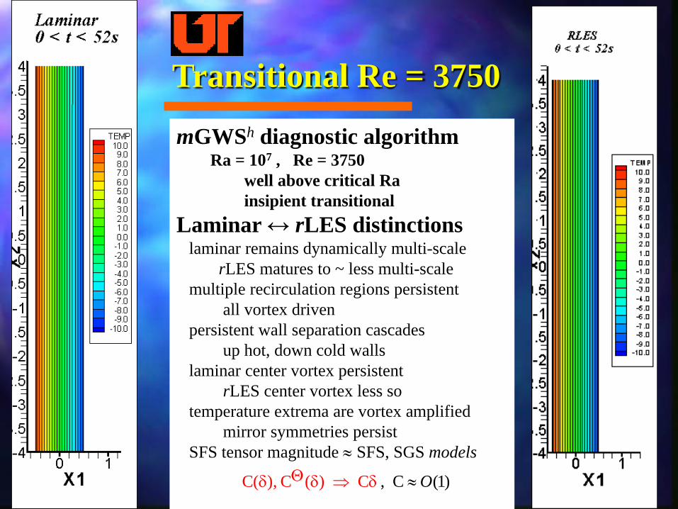
Transitional Re = 3750

mGWSh diagnostic algorithmRa = 107 , Re = 3750

well above critical Ra insipient transitional

Laminar ↔ rLES distinctionslaminar remains dynamically multi-scale

rLES matures to ~ less multi-scalemultiple recirculation regions persistent

all vortex drivenpersistent wall separation cascades

up hot, down cold wallslaminar center vortex persistent

rLES center vortex less sotemperature extrema are vortex amplified

mirror symmetries persist SFS tensor magnitude ≈ SFS, SGS models

, C (C( ), C ( ) 1C )OΘδ δ ⇒ ≈δ

Diagnostics, Transitional Re = 3750

Streamfunction, to scale Streamfunction with velocity vectors, 1×1 scale

rLES PDE System EBV ChallengerLES theory: filter δ permeates PDEs

filter cannot extend beyond a wallδ must be uniform (commutation error)

⇒ BCs for wall bounded flows ? !

Legacy LES closure: filter δ not in PDEsSGS models define: δ ⇒ δ(x, t)

Dual-filter resolution: gaussian + compactenergetic eddies do not touch wallsgaussian everywhere for |x - x(∂Ω)| > δ/2 ≈ h

Cij, CjΘ BCs vanishing Neumann @ |x| ~ δ/2

compact filter in wall layers |x - x(∂Ω)| < δ/2δ not in PDEs ⇒ wall-graded meshingvelocity BC is no slip wallSGS tensor closure required !

Vectors on vorticity

Gauss-compact filter interface

←h→

← δ →

Laminar ⇔ rLES Diagnostic, Re = 3750

Temperature Vorticity VorticityTemperature

State Variable Diagnostics, Re = 3750

Convection nonlinearity Stokes tensor Cross-stress tensor pair SFS tensor

State Variable Diagnostics, Re =3750

Convection + P Stokes tensor Cross-stress tensor pair SFS tensor

Turbulent Re = 11,900

mGWSh diagnosticsRa = 108

Re = 11,900well above critical Ra turbulent effects to dominate?

(not forced, comparison)Multi-scale flow evolution:

wall vortex rolls ⇒ wall jetwall jet layers unsteadytranslating thermal plumes

large eddies no longer existcenter region ⇒ homogeneous

essentially isothermalSFS tensor role more significant

Diagnostics, Turbulent Re = 11,900

Streamfunction, to scale Temperature with velocity vectors, 1×1 scale

mGWSh Diagnostics: Re = 3750, 11,900

Temperature, Ra=E7 Vorticity , Ra=E7 Vorticity, Ra=E8Temperature, Ra=E8

Analytic Diagnostics, Re Dependence

Wall-adjacent thermal transport velocity vector fields

Transitional Re = 3750:wall vortex rolls continuallycascade up/down vertical walls

Turbulent Re = 11,900:unsteady wall jets withtranslating thermal plumes

State Variable Diagnostics as f(Re)Cross-stress tensor pair spectral content distributions

Laminar ↔ rLESRe = 375

LaminarRe = 3750

TransitionalRe = 3750

TurbulentRe = 11,900

State Variable Diagnostics as f(Re)Convection shear

Re = 3750|ext| = 0.18

Re = 3750|ext| = 0.013

Re = 11,900|ext| = 1.40

Re = 11,900|ext| = 0.040

Cross-stress tensor pair shear

State Variable Diagnostics as f(Re)Stokes tensor viscous shear

Re = 3750|ext| = 0.015

Re = 3750|ext| = 0.0053

Re = 11,900|ext| = 0.033

Re = 11,900|ext| = 0.050

SFS tensor shear

Laminar, Re = 6850, 1500 time-steps @ ∆t = 0.02 sec (Sahu & Baker, 2007)

mGWSh optimal O(κh3) Validation

Analytic Diagnostic LES mGWSh

Analytic rLES theory: wavenumber asymptotics + deconvolutiongaussian filter measure δ permeates the rLES PDE system

resolved velocity solutions directly scaled by filter size ! ! convolution/deconvolution mathematically exact

analytic cross-stress tensor pair, symmetric, O(δ2) non-deviatoric, realizable, translation/Galilean invariantlinear harmonic PDEs, elliptic BCs ? ! modulo kinetic flux vector, not a priori dissipative !

O(δ4) sub-filter scale tensor function is trivialmust dissipate energy at unresolved scale threshold

analytic theory extents to thermal, mass transport ∀ Re without Prt, Sct

Analytic nonlinear SFS tensor closureSFS tensor theory is analytic in the continuum ! !

meets O(δ3) significance requirementsingle scalar coefficient O(1)dissipation spectrum ranges O(2h – 4h) ~ O(δ)

symmetric, nonlinear, non-positive definiteadmits backscatter ? !

laminar flow predictions unaffecteddoes not laminarize transitional Re flowturbulent Re ⇒ added significance !

Research Topics, Analytic rLES Theory

filter cannot extend beyond a wallfilter δ required uniform (commutation error)dual filter appears a resolution !

compact filter region requires SGS closureneed span only O(δ/2)

compact filter span ≤ δ/2

rLES theory PDE(δ) constraint

mGWSh rLES algorithm requires validationdecay of isotropic turbulence, of course ! !aerodynamic Reynolds tensor is not isotropic ! !

boundary layer/step wallwakes, trailing edges, cascadesduct flow transverse vortex structures

GPU-amenable 3-D mGWSh analytic rLES codeCFD Lab, JICS, NICS, USC, Trideum, Inc: S&T collaboration about to start !

Four Decades of Weak Form CFD⇒ Optimal Modified Continuous

Galerkin Diagnostic Analytic LES

Contributing UT CFD Lab dissertations:Osama Soliman (1978) Jin Kim (1987)Wilbert Noronha (1988) Joe Iannelli (1991)Jim Freels (1992) Paul Williams (1993)Subrata Roy (1994) Kwai Wong (1995)Jing Zhang (1995) David Chaffin (1997)Alexy Kolesnikov (2000) Sunil Sahu (2006)Marcel Grubert (2006) Next ( 2010 + ? )

+ COMCO contributors: Joe and Paul

THANK YOU ALL ! !