Confocal microscopyZeiss LSM 510 and Zeiss LSM 510 META

Visualisation of biological structures in 3D

Confocal Microscope

Features above and below the plane of focus fall outside the pinhole and appear black - producing a true optical section.

Upright Zeiss LSM 510 confocal microscope

Inverted Zeiss LSM 510 confocal microscope

Upright Zeiss LSM 510 META confocal microscope

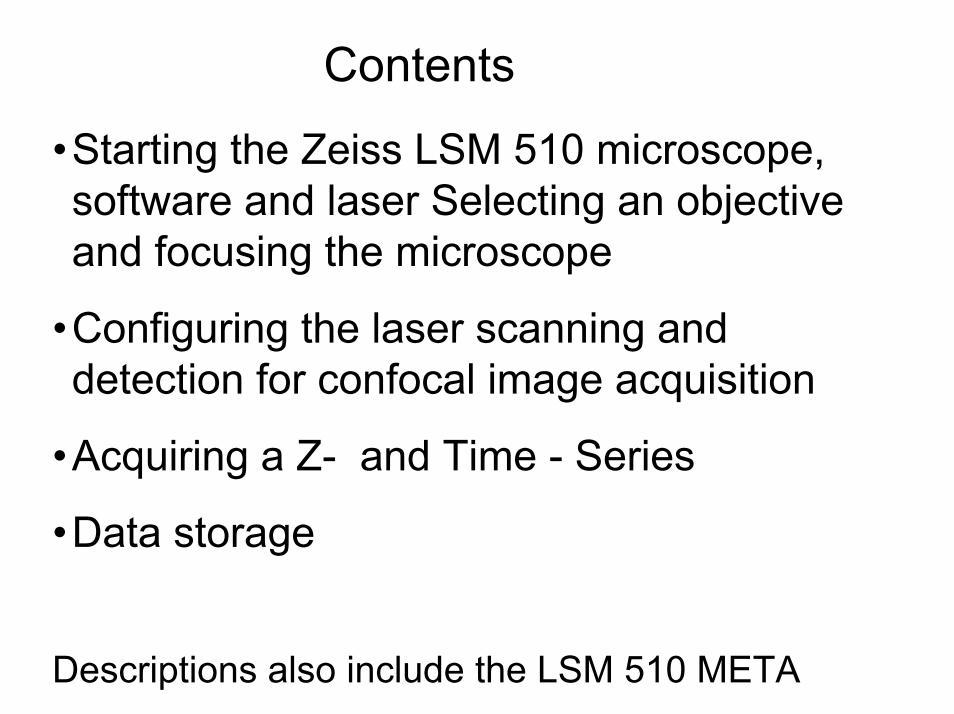
Contents

•Starting the Zeiss LSM 510 microscope, software and laser Selecting an objective and focusing the microscope

•Configuring the laser scanning and detection for confocal image acquisition

•Acquiring a Z- and Time - Series

•Data storage

Descriptions also include the LSM 510 META

Contents

•Starting the Zeiss LSM 510 microscope, software and laser

•Selecting an objective and focusing the microscope

•Configuring the laser scanning and detection for confocal image acquisition

•Acquiring a Z- and Time - Series

•Data storage

Start the Zeiss LSM 510 Confocal Microscope

1) First switch on the mercury lamp

2) Turn on the remote control switch

3) Wait for the computer to boot up and Login by simultaneously pressing the Ctrl, Alt and Delete keys

Starting the LSM 510 software

1) Double click the LSM 510 icon

2) Select “Scan New Images”

3) Select “Start Expert Mode”

Creating a database for acquired images

1) In the main menu File select New database

2) Select drive C or D: from pull down menu

3) Create a new directory for each session

1) Select Acquire

3) Switch required laser/s to Standby or On

Argon power should be set to about 60%

Turning on the lasers

2) Select Laser

For direct observationof transmitted light and fluorescence:

Set slider to “VIS” (push it in)

Change between direct observation and laser scanning

Upright Microscopes: Axioplan 2 imaging and Axioskop 2 FS

For laser scanningimage acquisition:

Set slider to “LSM” (pull slider out)

Change between direct observation and laser scanning

Inverted Microscope: Axiovert 200 M

Toggle between Vis and LSM button in main menu, automatic switching between direct observation and laser scanning (no slider)

Contents

•Starting the Zeiss LSM 510 microscope, software and laser

•Selecting an objective and focusing the microscope

•Configuring the laser scanning and detection for confocal image acquisition

•Acquiring a Z and Time -Series

•Data storage

Selecting an objective and focusing the microscope

1) Select Micro (Main menu: Acquire)(For Axioskop 2 FS these settings have to be adjusted manually)

3) Objective lens can be selected from a pull down menu by clicking onto the Objective button

2) Microscope settings can be stored and up to 8 buttons assigned for fast retrieval and adjustment

Focusing the microscope in fluorescence mode

Click onto Reflected Light to open the shutter of the HBO lamp

Fluorescence is observed by selecting the appropriate filter set in the pull down menu of Reflector

Focusing the microscope in transmitted mode

Click onto Transmitted Lightand move the slider to set the intensity of the HAL illumination

Use no reflector cube in the reflector turret, chose None

Contents

•Starting the Zeiss LSM 510 microscope, software and laser

•Selecting an objective and focusing the microscope

•Configuring the laser scanning and detection for confocal image acquisition

•Acquiring a Z- and Time - Series

•Data storage

Choosing the configuration

SINGLE TRACK MULTI TRACK

Simultaneous scanning only

Use for single, double and triple labelling

Use for double or triple labelling

Sequential scanning, line by line or frame by frame

When one track is active, only one detector and one laser is switched on. This dramatically reduces crosstalk.

ADVANTAGESFaster image acquisition

ADVANTAGES

DISADVANTAGES DISADVANTAGESSlower image acquisitionCross talk between channels

Configuration of the filters and storage of the track configurationsSINGLE TRACK - lasers scan simultaneously

1) Select Config in the Acquire menu

2) SelectSingle Track

3) Select the appropriate filters and activate the Channels

4) The Config button opens the pull down menu to load/store Track configurations

3) Click Excitation to select the laser and attenuation

Transmitted light image can also be generated. Transmission channel is usually set to white colour.

Applying a stored configuration and checking the settings

If you select Store by mistake, software will ask you, if you want to overwrite the configuration. ANSWER NO!

Each new login loads a predefined set of correct configurations.

5) Chose a configuration in the Track Configuration menu. Select Apply

The Spectra button opens a window to display the activated laser lines for excitation (colored vertical lines) and channels (colored horizontal bars)

6) To check for correct settings, click the Spectra button

Multi Track Configuration

3) Select a stored track from the pull down menu, click on Apply

This button stores only the highlighted single track or applies a single track.

1) Select Multi Track for sequential scanning

2) Select Config

Cy5-Cy3-FITC Multi TrackThree laser lines and channels activated sequentially

Excitation Detection

633 nm, using the META detector in Channel mode

543 nm

488 nm

Setting the parameters for scanning

1) Select Scan

3) Select the Frame Sizeas predefined number of pixels or enter your own values (e.g 300 x 600). Use Optimal for calculation of appropriate number of pixels depending on N.A. and λ.

The number of pixels influences the image resolution!

2) Select Mode

Setting the parameters for scanning

Note: When using a Axioskop 2 FS, indicate the Objective that is in use in the Scan Control window. This ensures correct calculation of pinhole, z-stack optimization etc.

Adjusting the scan speed

Adjust the scan speed - a higher speed with averaging results in the best signal to noise ratio. Scan speed 8 usually produces good results. Use 6 or 7 for superior images.

Choosing the Dynamic Range (8/12 Bit per pixel)

Select the dynamic range - 8 bit will give 256 gray levels, 12 Bit will give 4096 levels. Photoshop 5 will import 12 and 16 Bit images.

Publication quality images should be acquired using 12 Bit.

Channel Settings - Adjusting the Pinhole

Pinhole size = 1 Airy unit

0.8 “Airy units” produces the best signal : noise ratio

Pinhole adjustment changes the “Optical slice”.

When collecting multi channel images, adjust the pinholes so that each channel has the same “Optical Slice”.

This is important for colocalization studies.

2) Select Fast XYfor continuous fast scanning - useful for finding and changing the focus

Image Acquisition

1) Findautomatically pre-adjusts detector sensitivity

3) Stop blanks the laser beam and stops the scanning mirrors

Minimal Pixel Size determined by Nyquist Sampling

× NA

5

10

20

40

63

100

0.15

0.3

0.5

1.3 (oil)

1.4 (oil)

1.4 (oil)

1.03 µm

PIXEL SIZE

0.51 µm

0.31 µm

0.12 µm

0.11 µm

0.11 µm

Adjusting the field size (“XY”) to 56 µm with the 63× lens, would produce a pixel size of 0.1 µm

Brightness of image = Magnification2/NA2

Values are for scan zoom = 1.0

Field size can be adjusted by changing the objective magnification, or by optical zooming. Changing from 63 × to 100 × will reduce the field size, but will also reduce the amount of light available.

Optical Zooming

The image can also be rotated by selecting and dragging the bars

The level of zoom can be changed either by using the Zoom, Rotation & Offsetcontrol in Mode menu of the Scan Control, or by selecting Crop in the image menu.

Selecting gain and offset – Choosing a lookup table

1) Select Palette

2) Select Range Indicator

Red = Saturation (maximum)

Blue = Zero (minimum)

Scan Control – Setting Gain and Offset

Detector gain determines the sensitivity of the detector by setting the maximum limit

Amplifier Offset determines the minimum intensity limit

Amplifier Gain determines signal amplification

Saturation at the maximum →reduce Detector Gain

Saturation at the minimum increase Amplifier Offset

Gain set correctly

Offset set correctly

Gain

Offset

Amplifier Gain increases the whole signal, and the Amplifier Offset will need to be decreased.

Saturation of Signal Intensity with Laser Power

2% 4% 6% 8%Argon laser 488 nm % transmission

Sign

al In

tens

ity

Photobleaching is linear!

•Fluorophore saturates at 6% laser transmission

•Photobleaching is linear

Laser transmission should not be set higher than the saturation level.

Adjusting the Laser Intensity

1) Set Pinhole to 1 Airy unit

2) Set Detector Gain high

3) When the image is saturated, reduce AOTF transmission in the Excitation panel to reduce the intensity of the laser light at the specimen

Adjusting Gain and Offset

Both Detector Gain and Amplifier Offsetsaturated

1) Increase the Amplifier Offset until all blue pixels disappear, and then make it slightly positive.

2) Reduce the Detector Gain until the red pixels only just disappear.

Adjusting the Laser, Gain and Offset using aMulti Track Configuration

Each channel is selected independently by clicking on the colour button indicating the channel i.e. Ch2-T1 (Channel 2, Track 1). The laser power and all other parameters are optimised as described in the previous slides for each selected channel.

For accurate colocalisation, adjust each Pinhole so that each channel has the same Optical Slice

0.8 Airy units gives the best signal:noise ratio

Setting up Gain and Offset - Multi Track

1) Select Split XY in the Image window

2) In Palette, select Range indicator

3) Select each channel separately under Channels in the Scan control window and adjust the Laser intensity, Detector Gain, and Amplifier Offset as described previously.

Split

Line Averaging

2) Select Number for averaging. The more the better for the signal to noise ratio (max 16) in this case, each line will be scanned 4 times. But: Averaging increases the exposure time of the sample!!

Averaging improves the image by increasing the signal : noise ratio

Averaging can be achieved line by line, or frame by frame

1) Select Line or Frame under Mode in Scan Average within the Mode panel of the Scan Control window

Frame Averaging1) Select Frame

2) Select the Number for averaging - The more the better for signal to noise ratio (max 16). Continuous averaging is possible in this mode.

Frame averaging helps reduce photobleaching, but does not give quite such a smooth image. There is also a longer delay between each track when using “Multi Track”.

Continuous averaging has a Finish button which allows the scan currently in progress to be completed before stopping

Collecting an Averaged Image

In the Channels panel of the Scan Control window select Single. An averaged image will be collected.

Range indicator set to No Palette

1) Under Scan Average select the Number for the average.

Contents

•Starting the Zeiss LSM 510 microscope, software and laser

•Selecting an objective and focusing the microscope

•Configuring the laser scanning and detection for confocal image acquisition

•Acquiring a Z- and Time - Series

•Data storage

Scanning a Z-Series using Mark First/Last

NOTEFocusing can be achieved manually (preferred), or using Stage in the LSM menu if there is a motorized scanning table.

Focus

Increment

1) Select Z Stack

2) Start scanning using Fast XY or XY cont

3) Keep your eye on the image and move the focus to the beginning of the Z-Series, then select Mark First

4) Move the focus back in the opposite direction to the end of the Z-Series, then select Mark Last

5) X:Y:Z = 1:1:1 sets the Z-interval so that the voxel has identical dimensions in X, Y, and Z.

6) Start will initiate the acquisition of the Z-Stack. The acquisition can be stopped at any time.

Using Auto Z Brightness Correction

Auto Z provides an automatic gradual adjustment of Detector Gain, Amplifier Offset, Amplifier Gain, and Laser intensity setting between the first and last optical slice of a Z Stack.

1) After defining the Z position of the first and last optical slice activate Auto Z.

2) Move to the First Slice and adjust the parameter for the image acquisition in the Channels panel for each used channel as described in the previous slides. Then click on Set A to store the values.

3) Repeat the procedure after moving to the LastSlice. Click on Set B to store the parameters for the last slice.

4) The parameters for image acquisition will be gradually and linearly adjusted between the first and last slice of the Z Stack. Thus signal intensity and image quality is comparable throughout the Z Stack.

Confocal Z Sectioning Number of Sections for correct sampling

Optical thickness d depends on:

• Wavelength λ• Objective lens, N.A.• Refractive index n• Pinhole diameter P

d ~ P n λ / (N.A)2

~ 0.5 µm @ 63x1.4

Optimal: (no missing information @ minimal number of sections)

Slices overlap by the half of their thickness

„Nyquist-“ or Sampling- Theorem

Z Stack – Number of Slices and Increment

1) Select Z slice - the window Optical Slice will appear

2) Select Optimal interval the computer will calculate the optimum number of sections

3) Select Start

For more or less sections -adjust Num Slices

Z - Series using Z Sectioning

1) Select Z Stack

2) Select Z Sectioning

3) Select Line Sel

4) Select the large arrow button and position the XZ cut line

Z Sectioning – Setting Range

1) Decide whether to Keep Interval (number of slices will change) or Keep Slice (Intervalbetween slices will be adjusted)

2) Select Range and position bars to decide where the Z - Series begins and ends

3) Select Start for image acquisition

Vertical section of sample

Set limits for Z-Series

Viewing a Z - Series

In the image window

1) Select xy

2) Select Slice

3) Use scroll bar to view individual sections

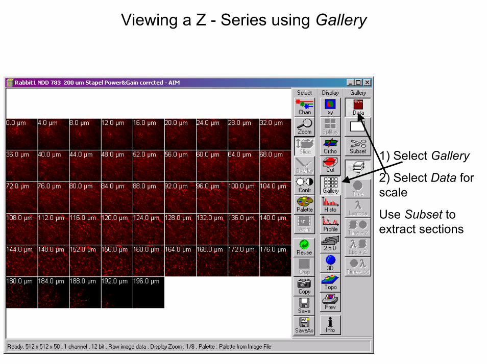
Viewing a Z - Series using Gallery

1) Select Gallery

2) Select Data for scale

Use Subset to extract sections

Viewing a Z- Series using Orthogonal Sections

1) Select Ortho

2) Select mouse (Select)

3) Using the mouse, position the cut lines.

To save orthogonal sections, select Export and save as contents of image window.

Selecting and Saving a Region of Interest (ROI)

1) Select Overlay and define shape of ROI

2) Extract region creates a Z-Stack from the ROI

3) Save data

Using a ROI for faster image acquisition and data saving1) Select EditROI from the LSM menu bar

2) Select Fit Frame Size to bounding Rectangle

3) Choose shape of ROI

4) Position and size the ROI in the image with the mouse

5) Start Scan

To remove ROI and overlay select blue bin or deactivate ROI. Closing the window only removes overlay, ROI is still active. Deactivate Use ROI in the LSM menu.

Multiple Regions of Interest1) Un-select Fit Frame Size to bounding Rectangle, Choose shapes of ROIs

4) Position and size the ROIs with mouse

5) Start ScanTo remove ROIs and overlay select blue bin or deactivate ROIs. Closing the window only removes overlay, ROIs are still active. Deactivate Use ROI in the LSM menu.

Time Series

1)Set up scanning parameters for image acquisition as described in previous slides

2)Select TimeSeries from the LSM menu

3)Enter the Number of cycles

4)For a Time Delay between image acquisition select min, sec or ms and set time with the slider

5)Select Start T to start image acquisitionStart and Stop of the Time Series using Time as trigger uses the system time!

Viewing a Time Series of a Z StackZ Sections for any time

Time points for any Z Section

Both Z sections and time series

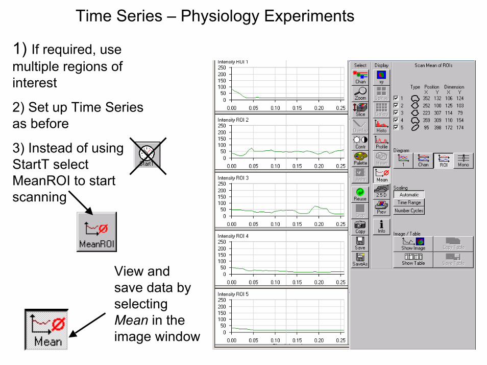
Time Series – Physiology Experiments

1) If required, use multiple regions of interest

2) Set up Time Series as before

3) Instead of using StartT select MeanROI to start scanning

View and save data by selecting Mean in the image window

Imaging a large area using Tile Scan

This function is only available with a motorized stage

1)Select Stage on LSM menu

2) Enter the Tile Numbers

3) Select Start

The maximum size is 4096 x4096 pixels

Any position can then be marked and a single image acquired by selecting Move to and then single

Tiled Image

Contents

•Starting the Zeiss LSM 510 microscope, software and laser

•Selecting an objective and focusing the microscope

•Configuring the laser scanning and detection for confocal image acquisition

•Acquiring a Z- and Time - Series

•Data storage

Saving Data - Using Database

1) Select Save or Save as on image window or LSM menu bar

2) Enter file name and notes if required

3) Select OK

Saving Data – Using Export

1) Select File from LSM menu

2) Select Export

3) Select Image type

4) Select Single image with raw data (No overlay or Look up table etc. is saved), Series with raw data, or Contents of the image window (Saves the image as shown on the screen)

5) Select Save as type

“Tif - Tagged image File” is OK for 8 bit - use “Tiff -16 bit” for 12 bit acquired images (Most other software will not recognize 12 bit)

Shut Down Procedure

1. Go to: Acquire in the LSM menu - Laser – and deactivate all Lasers by clicking Off to switch off Lasers

2. Go to File - Exit to leave LSM 510 program3. Shut down the computer 4. Turn off the remote control box5. Switch off the mercury vapour lamp.

This guided tour is based on work done by

Peter JordanICRF

LondonUnited Kingdom

edited and complemented byEva Simbürger and Solveig Hehl

Carl Zeiss Jena GmbH