No-reference image blur assessment using …live.ece.utexas.edu/publications/2011/Chen_eurasip_2011.pdfRESEARCH Open Access No-reference image blur assessment using multiscale gradient

RESEARCH Open Access

No-reference image blur assessment usingmultiscale gradientMing-Jun Chen* and Alan C Bovik

Abstract

The increasing number of demanding consumer video applications, as exemplified by cell phone and other low-cost digital cameras, has boosted interest in no-reference objective image and video quality assessment (QA)algorithms. In this paper, we focus on no-reference image and video blur assessment. We consider natural scenesstatistics models combined with multi-resolution decomposition methods to extract reliable features for QA. Thealgorithm is composed of three steps. First, a probabilistic support vector machine (SVM) is applied as a roughimage quality evaluator. Then the detail image is used to refine the blur measurements. Finally, the blurinformation is pooled to predict the blur quality of images. The algorithm is tested on the LIVE Image QualityDatabase and the Real Blur Image Database; the results show that the algorithm has high correlation with humanjudgments when assessing blur distortion of images.

Keywords: No-reference blur metric, Gradient histogram, Multi-resolution analysis, Information pooling

1. IntroductionWith the rapid and massive dissemination of digitalimages and videos, people live in an era replete withdigitized visual information. Since many of these imagesare of low quality, effective systems for automatic imagequality differentiation are needed. Although there are avariety of effective full-reference (FR) quality assessment(QA) models, such as the PSNR, the structural similarity(SSIM) index [1,2], the visual information fidelity index[3], and the visual signal-to-noise ratio (VSNR) [4],models for no-reference (NR) QA have not yet achievedperformance that is competitive with top performing FRQA models. As such, research in the area of blind orNR QA remains quite vital.There are many artifacts that may occur in a distorted

image, such as blocking, ringing, noise, and blur. UnlikeFR QA, where a reference is available to test against anydistortion, NR QA approaches generally seek to captureone or a few distortions. Here we are mainly concernedwith NR blur assessment, which remains an importantproblem in many applications. Generally, humans tendto conclude that images with more detail are of higherquality. Of course, the question is not so simple, since

blur can be space-variant, may depend on depth-of-field(hence effect foreground and background objects differ-ently), and may depend on what is being blurred in theimage.A number of NR blur indices have been developed,

the majority of which are based on the analyzing lumi-nance edges. For example, the sharpness measurementindex proposed by Caviedes and Gurbuz [5] is based onlocal edge kurtosis. The blur measurement metric pro-posed by Marziliano et al. [6] is based on analyzing ofthe width or spread of edges in an image, while theirother work is based on an analysis of edges and adjacentregions in an image [7]. Chuang et al. [8] evaluate blurby fitting the image gradient magnitude to a normal dis-tribution, while Karam et al. develop a series of blurmetrics based on the different types of analysis appliedto edges [9-13].Other researchers have studied blur assessment by fre-

quency domain analysis of local DCT coefficients [14],and of image wavelet coefficients [15-17]. These meth-ods generally rely on a single feature to accomplish blurassessment. While some of these algorithms deploy sim-ple perceptual models in their design [7,9,11,12,17], atheme that we extend in our approach. Specifically, weuse a model of neural pooling of the responses of corre-lated neuronal populations in the primary visual cortex

* Correspondence: [email protected] of Electrical & Computer Engineering, Laboratory for Image andVideo Engineering, The University of Texas at Austin, Austin, TX, USA

Chen and Bovik EURASIP Journal on Image and Video Processing 2011, 2011:3http://jivp.eurasipjournals.com/content/2011/1/3

© 2011 Chen and Bovik; licensee Springer. This is an Open Access article distributed under the terms of the Creative CommonsAttribution License (http://creativecommons.org/licenses/by/2.0), which permits unrestricted use, distribution, and reproduction inany medium, provided the original work is properly cited.

mailto:[email protected]

http://creativecommons.org/licenses/by/2.0

[18]. The use of multiple features combined usingmachine learning methods has also been studied [19,20].We are also inspired by recent progress on utilizing

natural scene statistics (NSS) to improve image proces-sing algorithms. Natural images obey specific statisticallaws that, in principle, might be used to distinguish nat-ural images from artificially distorted images [21]. Inthis regard, images that are blurred beyond a norm (e.g.,more than the band limit provided by the normalhuman lens at optical center) may measurably departfrom statistical “naturalness.” By this philosophy, wemay anticipate that NR blur indices can be designedthat analysis image statistics. Indeed, Sheikh et al. suc-cessfully used NSS for NR QA of JPEG-2000 distortedimages [22]. In their work, specific NSS features drawnfrom the gradient histogram were used.Here we develop a new blur assessment index that

operates in a coarse-to-fine manner. First, a coarse blurmeasurement using gradient histogram features isdeployed that relies on training a probabilistic supportvector machine (SVM). A multi-resolution analysis isthen used to improve the blur assessment, deploying amodel of neural pooling in cortical area V1 [18]. Theoverall algorithm is shown to agree well with humansubjectivity.The rest of the paper is organized as follows: Section 2

describes the way in which NSS are used. Section 3describes the coarse-scale NR blur index. Section 4extends the metric using multi-resolution analysis. Sec-tion 5 explains the use of the neural pooling model. Theoverall NR blur index is evaluated in Section 6, and con-cluding remarks are given in Section 7.

2. Natural image statisticsRecent research on natural image statistics have shownthat natural scenes belong to a small set in the space ofall possible image signals [23]. One example of a naturalscene property is the greater prevalence of strong imagegradients along the cardinal (horizontal and vertical)orientations, in images projected from both indoor andoutdoor scenes. A number of researchers have devel-oped statistical models that describe generic naturalimages [19] (including images of man-made scenes).Although images of real-world scenes vary greatly in

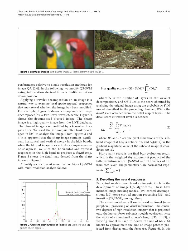
their absolute color distributions, image gradients gener-ally have heavy tailed distributions [24]. Natural imagegradient magnitudes are mostly small, yet take largevalues significantly more often than a Gaussian distribu-tion. This corresponds to the intuition that images oftencontain large sections of smoothly varying intensities,interrupted by occasional abrupt changes at edges orocclusive boundaries. Blurred images do not have sharpedges, so the gradient magnitude distribution shouldhave greater relative mass at small or zero values. By

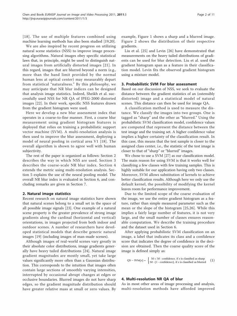
example, Figure 1 shows a sharp and a blurred image.Figure 2 shows the distribution of their respectivegradients.Liu et al. [25] and Levin [26] have demonstrated that

measurements on the heavy tailed distributions of gradi-ents can be used for blur detection. Liu et al. used thegradient histogram span as a feature in their classifica-tion model. Levin fits the observed gradient histogramusing a mixture model.

3. Probabilistic SVM For blur assessmentBased on our discussion of NSS, we seek to evaluate thedistance between the gradient statistics of an (ostensiblydistorted) image and a statistical model of naturalscenes. This distance can then be used for image QA.A classification method is used to measure the dis-

tance. We classify the images into two groups. One istagged as “sharp” and the other as “blurred.” Using theprobabilistic SVM classification model, confidence valuesare computed that represent the distance between thetest image and the training set. A higher confidence valueimplies a higher certainty of the classification result. Inthis case, this means that the test sample is closer to theassigned class center, i.e., the statistic of the test image iscloser to that of “sharp” or “blurred” images.We chose to use a SVM [27] as our classification model.

The main reason for using SVM is that it works well forclassifying a few classes with few training samples. This ishighly suitable for our application having only two classes.Moreover, SVM allows substitution of kernels to achievebetter classification results. Although here we only use thedefault kernel, the possibility of modifying the kernelleaves room for performance improvement.Due to the limited scope of the coarse evaluation of

the image, we use the entire gradient histogram as a fea-ture, rather than simple measured parameter such as themean or the slope of the histogram [25,26]. While thisimplies a fairly large number of features, it is not verylarge, and the small number of classes ensures reason-able computation. We describe the training procedureand the dataset used in Section 6.After applying probabilistic SVM classification on an

image, a label that indicates its class and a confidencescore that indicates the degree of confidence in the deci-sion are obtained. Then the coarse quality score of theimage is defined simply as:

QS − SVM(x) ={

50 + 50 · confidence, if x is classified as sharp50 · (1 - confidence), if x is classified as blurred (1)

4. Multi-resolution NR QA of blurAs in most other areas of image processing and analysis,multi-resolution methods have afforded improved


Page 2 of 11

performance relative to single-resolution methods forimage QA [2,4]. In the following, we modify QS-SVMusing information derived from a multi-resolutiondecomposition.Applying a wavelet decomposition on an image is a

natural way to examine local spatio-spectral propertiesthat may reveal whether the image has been modified.For example, Figure 3 shows a sharp natural imagedecomposed by a two-level wavelet, while Figure 4shows the decomposed blurred image. The sharpimage is a high-quality image from the LIVE database.The blurred image was modified by a Gaussian low-pass filter. We used the 2D analysis filter bank devel-oped in [28] to analyze the image. From Figures 3 and4, it is apparent that the sharp image contains signifi-cant horizontal and vertical energy in the high bands,while the blurred image does not. As a simple measureof sharpness, we sum the horizontal and verticalresponses in the high band to produce a detail map.Figure 5 shows the detail map derived from the sharpimage in Figure 3.A quality (or sharpness) score that combines QS-SVM

with multi-resolution analysis follows:

Blur quality score = (QS - SVM)r0

N∏i=1

(DSi)ri (2)

where N is the number of layers in the waveletdecomposition, and QS-SVM is the score obtained byanalyzing the original image using the probabilistic SVMmodel described in the preceding. Further, DSi is thedetail score obtained from the detail map of layer i. Thedetail score at wavelet level i is defined:

DSi =

Wi∑m=1

Hi∑n=1

∇i(m, n)

Wi · Hi

(3)

where Wi and Hi are the pixel dimensions of the sub-band image that DSi is defined on, and ∇i(m, n) is thegradient magnitude value of the subband image at coor-dinate (m, n).Blur quality score is the final blur evaluation result,

which is the weighted (by exponents) product of thefull-resolution score QS-SVM and the values of DSfrom each layer. The parameters ri are normalized expo-

nents:∑N

i=0ri = 1 .

5. Decoding the neural responsesPerceptual models have played an important role in thedevelopment of image QA algorithms. These haveincluded image masking models [29], cortical decompo-sitions [30], extra-cortical motion processing [31], andfoveation [29,32-34], among others.The visual model we will use is based on foveal (non-

peripheral) processing of visual information. The centraltwo degrees of high-resolution imagery that is projectedonto the human fovea subtends roughly equivalent twicethe width of a thumbnail at arm’s length [35]. In [9], aviewing model is used to derive the use of 64 × 64blocks to approximate the size of image patches pro-jected from display onto the fovea (see Figure 6). In this

Figure 1 Exemplar images. Left: blurred image A. Right: Bottom: Sharp image B.

Figure 2 Gradient distributions of images. (a) Solid line and (b)dashed line in Figure 1.


Page 3 of 11

viewing model, a subject is assumed to be sitting infront of a 24” × 18” LCD screen with a resolution of1680 × 1050 pixels. The width of foveal vision at arm’slength is assumed to be about 1.2”, while the viewingdistance is assumed to fall in the range 36-54”

(approximately 2-3 times the screen height). The armlength of the viewer is assumed to be 33 in.. Then, thewidth of span of foveal vision on the screen fallsbetween 76 (1050/18 × 1.31) and 116 (1050/18 × 2)pixels.

Figure 3 Wavelet decomposition of natural image. Top left: low band response. Top right: horizontal high band response. Bottom left:vertical high band response. Bottom right: high band response.

Figure 4 Wavelet decomposition of blurred image. Top left: low band response. Top right: horizontal high band response. Bottom left:vertical high band response. Bottom right: high band response.


Page 4 of 11

Since a block size of 2n along each dimension facilitatesoptimization and allows better memory management(aligned memory allocation), the choice of a 64 × 64 blocksize is a decent approximation. We then apply the blur QAmethod described in Section 4 on each of these blocks.When a human observer studies an image, thus arriv-

ing at a sense of its quality, she/he engages in a processof eye movement, where visual saccades place fixations atdiscrete points on the image. Image quality is largely

decided by information that is collected from these fovealregions, with perhaps, additional information drawn fromextra-foveal information. The overall perception of qual-ity drawn from these fixated regions might be describedas “attentional pooling,” by analogy with the aggregationof information from spatially distributed neurons. Weutilize the results of a study conducted by Chen et al.[18] to formulate such an attentional pooling strategy. Inthis study, the authors examined the efficacy of differentpatch pooling strategies in a primate undergoing a visual(Gabor) target detection task.The authors of [18] used voltage sensitive dyed images to

measure the population responses in primary visual cortexof monkeys performing a demanding visual target detectiontask. Then, they evaluated the effects of different decodingstrategies in predicting the target pattern from measuredneural responses in primary visual cortex. The pooling pro-cess they considered used a linear summation model:

Xpooled =n∑

i=1

wixi (4)

where wi is the weight applied to the neuronal ampli-tude response xi.The pooling rules they studied are as follows:

1. Maximum average amplitude: wi ≠ 0 only for thepatch having maximum average neuronal responseamplitude.

Figure 5 Detail map computed from image in Figure 3.

Figure 6 The setting of the viewing model.


Page 5 of 11

2. Maximum d’: wi ≠ 0 only for the patch havingmaximum d’3. Maximum amplitude: wi ≠ 0 only for the site withmaximum amplitude in a given trial4. Mean amplitude: wi = 1/n5. Weighted average amplitude: wi is proportional tothe average amplitude response of xi6. Weighted d’: wi is proportional to d’7. Optimal

where d’ is the SNR of the neuronal responses acrosstrials:

d′ = |ES − EN|/√

σS2 + σN

2

2(5)

where ES is the mean response amplitude in targetpresent trials (signal trials), EN is the mean amplitude ofthe response in target-absent trials (noise trials) and sS

and sN are the corresponding standard deviations. The“optimal” pooling 7 is obtained under the assumptionthat the neuronal response at each site is Gaussian dis-tributed and independent across trials (although notacross space and time within a trial). The optimal set ofweights is defined as the product of the inverse of theresponse covariance matrix the vector of mean differ-ences in response between the signal and noise trials.Their experimental result is shown in Figure 7.From Figure 7, we can see that the maximal average

pooling rules (Rules 1 and 2) perform better than thetrial maximum (Rule 3), average pooling rules (Rule 4)and weighted pooling rules (Rules 5 and 6). Whenapplying analogous pooling rules to the image blurassessment problem, we observe that since distinct sig-nal and noise trials do not exist in our case (and in any

case the Gaussian assumption is questionable), so wecannot apply the optimal pooling rule (Rule 7). Further,the SNR d’ is not available as required by Rules 2 and 6.Hence, we choose the maximum average amplitude asour pooling rule. The slight difference here is that witha single (algorithmic) “trial” an average amplitude valueis not available, while the maximum amplitude (Rule 3)is unreliable. Instead, we use the average of the maxi-mum p% of responses as a pooling strategy. The poolingstrategy was applied only on activated neurons; hencewe applied the pooling only on activated blocks, where ablock was taken to be activated if the mean of the lumi-nance values in the block is higher than 20. Therefore,the final blur quality score is calculated as

Blur quality score = (QS − SVM)r0 ∗N∏

i=1

(Pool(DSi)

)ri (6)

where

Pool(DSi) =∑n

k=1wkiDSki (7)

where DSki is the detail response of block k from layeri, and wki = 1/p if the detail responses of block k inlayer i belong to the largest 10% of detail responses ofall activated blocks in the layer; otherwise wki = 0. Here,p is nominally set to 10. The blocking analysis and pool-ing are only applied on the multi-resolution part, sincethe NSS mentioned in Section 2 are based on the statis-tics of whole images.

6. Experiments and resultsThe LIVE image quality database [36] and the real blurimage Database [37] were used to evaluate the perfor-mance of our algorithm. The experiments in Sections6.1-6.3 were conducted on the LIVE database to gaininsights into the performance of algorithms that com-bine different blur assessment factors. The performancesare also compared to the performance of multi-scaleSSIM (or MS-SSIM, a popular and effect FR QAmethod).Then in Section 6.4, the Real blur database (586

Images) is used as a challenging test by which we com-pare our results with other NR QA blur metrics. TheLIVE image database includes DMOS subjective scoresfor each image and several types of distortions. Theexperiment was performed only on the blur images (174images). All of the images in the LIVE database areblurred globally. Samples of these images are shown inFigure 8. A total of 760 images were used for testing.

6.1. Performance of SVM ClassificationTo train the coarse SVM classifier, we used 240 trainingsamples which were marked as “sharp” or “blurred.” The

Figure 7 Comparison of detection sensitivity of candidatepooling rules. Asterisks indicate rules with performancesignificantly different from the optimal (bootstrap test, p < 0.05).


Page 6 of 11

training samples were randomly chosen and some ofthem are out-of-focus images. Due to the unbalancedquality of the natural training samples (there were moresharp images than naturally blurred images), we applieda gaussian blur to some of the sharp samples to gener-ate additional blurred samples. The final training setincluded 125 sharp samples and 115 blurred samples.The training and test sets do not share content.When tagging samples, if an original image’s quality

was mediocre, the image was duplicated; one copymarked as “blurred” and the other marked as “sharp,”with both images used for training. This procedure pre-vents misclassifications arising from marking mediocreimage as “sharp” or “blurred.” This duplication wasapplied to lower the confidence when classifying med-iocre samples.Note that DMOS scores of these images we are not

required to train the SVM. Images were simply taggedas “blurred” or “sharp” to train the SVM. Likewise, theoutput of the probabilistic SVM model is a class type("blurred” or “sharp”) and a confidence level. The classtype and confidence level are used to predict the imagequality score.The algorithm was evaluated against the LIVE DMOS

scores using the Spearman rank order correlation coeffi-cient (SROCC). The results are shown in Table 1.

In Table 1, QS-SVM means blind blur QA usingprobabilistic SVM, PSNR means peak signal to noiseratio, and MS-SSIM means multi-scale structure similar-ity index. To obtain an objective evaluation result, wecompared our method to FR methods tested on thesame database as in [4,38].As can be seen, the coarse algorithm QS-SVM deliv-

ered lower SROCC scores than the FR indices, althoughthe results are promising. Of course, QS-SVM is nottrained on DMOS scores, hence does not fully capturethe perceptual elements of blur assessment.

6.2. Performance with multi-resolution decompositionWe began by estimating which layers of the waveletdecomposition achieve the best QA result on the LIVEdatabase. We found the correlations between the DS

Figure 8 Sample images from the LIVE image quality database. From top-left to bottom-right, increasing Gaussian blur is applied.

Table 1 Comparison of the performance of VQAalgorithms

Prediction model SROCC

QS-SVM 0.6136

PSNR (FR) 0.7729

VSNR (FR) 0.932

MS-SSIM (FR) 0.9425


Page 7 of 11

scores and human subjectivity for each layer. The per-formance numbers are shown in Table 2.In Table 2, DS0 is the detail score computed from the

original image. The experiment shows the SROCC scoreof DS1 to be significantly higher than for the otherlayers. The detail map at this middle scale appears todeliver a high correlation with human impression ofimage quality.Next we combined the QA measurement in different

layers, omitting level 3 because of its poor performance.Table 3 shows the results of several combinations ofalgorithms. The parameters ri of each combination weredetermined by regression on the training samples.Table 3 shows that, except for combination with QS-

SVM, all other combinations with DS1 did not achievehigher performance than using only DS1. This result isconsistent with our other work in FR QA, where wehave found that mid-band QA scores tend to scorehigher than low-band or high-band scores. Adding morelayers did not improve performance here. The highestperformance occurs by combining DS1 with QS-SVM(r0 = 0.610, r1 = 0.390), yielding an impressive SROCCscore of 0.9105. Combination QS-SVM with DS2 (r0 =0.683, r2 = 0.317) also improved performance relative toDS2, suggesting that QS-SVM and the DS scores offercomplementary measurements.

6.3. Performance with pooling strategyWe studied the performance of different pooling rules inour system. The system is described by (6), using maxi-mum p% pooling, average pooling (Rule 4 in Section 5),and weighted pooling (Rule 5 in Section 5), applied toQS-SVM·DS1. Using tenfold cross-validation with fixedparameters r0 = 0.610 and r1 = 0.390, the performanceattained is given in Table 4. Table 4 shows that the

performance of using different pooling rules in our sys-tem is consistent with the results found in [18]. Themaximum p% pooling method improves the perfor-mance (the SROCC score is increased from 0.9004 to0.9248).All parameters in our system were kept fixed (p = 10,

r0 = 0.610 and r1 = 0.390) to enable fair comparisonswith other algorithms. The number p came from cross-validation across two databases. Table 5 illustrates thefinal performance of our algorithm as compared toother NR and FR blur metrics. The performance of ouralgorithm is better than PSNR and very close to CPBD[10] and to FR QA models when conducted on theblurred image portion of the LIVE Image Quality Data-base The plot of predicted objective quality (followinglogistic regression) against DMOS scores from the LIVEImage Quality Database is shown in Figure 9.

6.4. Challenging blur databaseOur foregoing experiments on the LIVE database wereby way of algorithm design and tuning, and not perfor-mance verification. To verify the performance of ouralgorithm, we conducted an experiment on a realblurred image database. The database contains 585images with resolutions ranging from 1280 × 960 to2272 × 1704 pixels.The images in this database were taken by consumer

cameras and are classified into five classes as“Unblurred” (204 images), “Out-of-focus” (142 images),“Simple Motion” (57 images), “Complex Motion” (63images) and “Other” (119 images). The images in the

Table 2 QA performance using different layers


QS-SVM 0.6136

DS0 0.6583

DS1 0.8884

DS2 0.7733

DS3 0.5587

Table 3 QA performance using different combinations oflayers


DS0·DS1 0.8884

DS1·DS2 0.8884

QS-SVM·DS1 0.9105

QS-SVM·DS1·DS2 0.9105

QS-SVM·DS2 0.8428

Table 4 QA performance numbers by tenfold cross-validation

Pooling rule SROCC

Maximum p% 0.9248

Average 0.9004

Weighted 0.9080

Different pooling rules were applied on the blurred image portion of the LIVEImage Quality Database

Table 5 Summary of QA performance of differentalgorithms on the blurred image portion of the LIVEImage Quality Database


QS-SVM 0.6136

PSNR (FR) 0.7729

QS-SVM·DS1 0.9105

QS-SVM·Pool(DS1) 0.9352

VSNR (FR) 0.932

MS-SSIM (FR) 0.9425

CPBD 0.9430


Page 8 of 11

“Out-of-focus” (142 images), “Simple Motion” (57images), “Complex Motion” (63 images) and “Other”(119 images). The images in the “Out-of-focus” class areglobal out-of-focus images. The “Simple Motion” classhas images that are blurred because of close-to-linearcamera movements and the “Complex Motion” class has

images which are blurred because of the more complexmotion paths. Finally, the “Other” class includes anyother types of degradation. It may include any combina-tion of the main classes. For instance, the image withlocalized out-of-focus blur (mixed “Unblurred” and“Out-of-focus”) was classified into the “Other” class.Sample images are shown in Figure 10. The raw MOSscores of the database are provided. We eliminated 20%(maximum 10% and minimum 10%) of the grades oneach image as outliers, so that the average (trimmedmean) of the 80% grades was used as the MOS score ofeach image.We used tenfold cross-validation and report the

SROCC numbers from applying several different poolingrules. As shown in Table 6, the maximum p% poolingmethod yields the best performance (0.5858). Althoughthe improvement is not significantly large, this methodshowed the best performance on both databases.By examining the experimental results from the LIVE

Image Quality Database and the Real Blur Image Data-base, we found that there is a significant performancedifference of the models on these two databases. TheLIVE database includes synthetically and globallyblurred sample images. The task of performing QA on aglobally blurred image is less complex and harder torelate to perceptual models. On LIVE, our proposed

Figure 9 Plot of predicted objective scores versus DMOS fromlive image quality database.

Figure 10 Sample images from the real blur database. Top left: Out-of-focus image. Top right: Simple motion blur. Bottom left: Complexmotion blur. Bottom right: Others (partial blur case).


Page 9 of 11

method of pooling showed significant improvement(from 0.9 to 0.925). However, on the Real Blur Database,where the blurs are more complex, possibly nonlinear,and spatially variant, blur perception is more complexand probably more correlated with content (e.g., what isblurred in the image?). By example, in the partiallyblurred image shown in Figure 10 (bottom right), therating is likely highly affected by image content, objectpositioning, probable viewer fixation, and so on.When comparing the performance of our proposed

algorithm with other blur assessment algorithms, werefer to the work conducted by Ciancio et al. [20]. Inthis work, they provided performance levels several algo-rithms, including a frequency-domain blur index [14], awavelet-based blur index [15], a perceptually motivatedblur index [7], a blur index using a human visual system(HVS) model [11], a local phase coherence blur metric[16], and their own Multi-Features Neural NetworkClassifier (MFNNC) blur metric [20]. The performanceof CPBD [10] is also included. The performance resultsare shown in Table 7.Table 7 shows that our proposed blur QA model deli-

vers the best performance amongst the algorithms com-pared. Although the improvement does not achievestatistical significance as compared with other top-per-forming models, it consistently shows better perfor-mance across a large number of images and acrossdatabases. A scatter plot of the scores delivered by ourmodel (following logistic regression) against the MOSscores from the Real Blur Database is shown in Figure11 showing very good general agreement. Many of theimages, such as Figure 12, contain difficult high level

content whose interpretation may depend on the obser-vers’ preferences regarding composition (and that of thephotographer).

7. ConclusionThe main contributions of this work are as follows.First, we found that the statistics of the image gradienthistogram and a detail map from the image waveletdecomposition can be combined to yield good NR blurQA performance. Second, our results discuss that a per-ceptually motivated pooling strategy can be used toimprove the NR blur index on assessing the blur images.Performance was demonstrated on the LIVE Image

Quality Database and the Real Blur Image Database. As

Table 6 Blur QA performance of applying differentpooling rules on real blur database

Pooling rule SROCC

Maximum p% 0.5858

Average 0.5604

Weighted 0.5542

Table 7 Blur QA performance of different algorithms onreal blur database

Algorithm SROCC

Frequency domain metric* 0.494

Wavelet-based metric* 0.524

Perceptual metric* 0.336

HVS based metric* 0.474

Local phase coherence metric* 0.523

MFNNC metric* 0.564

Proposed algorithm 0.586

CPBD 0.501

Algorithms marked by asterisk indicates their performance was reported in[20]

Figure 11 Plot of predicted objective score versus MOS scoreof real blur image database.

Figure 12 Subjects give higher quality to this image MOS is3.98 (scale from 0 (worst) to 5 (best)), but our algorithm giveslow objective score to this image.


Page 10 of 11

compared with other NR blur metrics, our methodyields competitive performance with reasonablecomplexity.

AbbreviationsQA: quality assessment; SVM: support vector machine; FR: full-reference;SSIM: structural similarity; VSNR: visual signal-to-noise ratio; NSS: naturalscene statistics; SROCC: Spearman rank order correlation coefficient; HVS:human visual system; MFNNC: multi-features neural network classifier.

Competing interestsThe authors declare that they have no competing interests.

Received: 15 September 2010 Accepted: 19 July 2011Published: 19 July 2011

References1. Wang Z, Bovik AC, Sheikh HR, Simoncelli EP: Image quality assessment:

from error visibility to structural similarity. IEEE Trans Image Process 2004,13(4):600-612.

2. Wang Z, Simoncelli EP, Bovik AC: Multi-scale structural similarity for imagequality assessment. IEEE Asilomar Conf. Signals, Systems, and Computers2003, 1398-1402.

3. Sheikh HR, Bovik AC: Image information and visual quality. IEEE TransImage Process 2006, 15(2):430-444.

4. Chandler DM, Hemami SS: VSNR: a wavelet-based visual signal-to-noiseratio for natural images. IEEE Trans Image Process 2007, 16(9):2284-2298.

5. Caviedes JE, Gurbuz S: No-reference sharpness metric based on localedge kurtosis. IEEE International Conference on Image Processing, Rochester,NY 2002.

6. Marziliano P, Dufaux F, Winkler S, Ebrahimi T: A no-reference perceptualblur metric. International Conference on Image Processing, Rochester, NY2002.

7. Marziliano P, Dufaux F, Winkler S, Ebrahimi T: Perceptual blur and ringingmetrics: application to JPEG2000. Signal Process Image Commun 2004,19(2):163-172.

8. Chung Y, Wang J, Bailey R, Chen S, Chang S: A nonparametric blurmeasure based on edge analysis for image processing applications. IEEEConf Cybern Intell Syst 2004, 1:356-360.

9. Narvekar ND, Karam LJ: A no-reference perceptual image sharpnessmetric based on a cumulative probability of blur detection. InternationalWorkshop on Quality of Multimedia Experience 2009.

10. Narvekar ND, Karam LJ: A no-reference image blur metric based on thecumulative probability of blur detection (CPBD). IEEE Trans Image Process2011.

11. Ferzli R, Karam LJ: A human visual system based no-reference objectiveimage sharpness metric. IEEE International Conference on Image Processing,Atlanta, GA 2006.

12. Ferzli R, Karam LJ: A no-reference objective mage sharpness metric basedon just-noticeable blur and probability summation. IEEE InternationalConference on Image Processing, San Antonio, TX 2007.

13. Varadarajan S, Karam LJ: An improved perception-based no-referenceobjective image sharpness metric using iterative edge refinement. IEEEInternational Conference on Image Processing, Chicago, IL 1998.

14. Marichal X, Ma WY, Zhang H: Blur determination in the compresseddomain using DCT information. IEEE International Conference on ImageProcessing, Kobe, Japan 1999.

15. Tong H, Li M, Zhang H, Zhang C: Blur detection for digital images usingwavelet transform. IEEE International Conference on Multimedia and EXPO2004, 1:17-20.

16. Ciancio A, Targino AN, da Silva EAB, Said A, Obrador P, Samadani R:Objective no-reference image quality metric based on local phasecoherence. IET Electron Lett 2009, 45(23):1162-1163.

17. Wang Z, Simoncelli EP: Local phase coherence and the perception ofblur. Advances in Neural Information Processing Systems MIT Press,Cambridge; 2004, 786-792.

18. Chen Y, Geisler WS, Seidemann E: Optimal decoding of correlated neuralpopulation responses in the primate visual cortex. Nat. Neurosci 2006,9:1412-1420.

19. Narwaria M, Lin W: Objective image quality assessment based on supportvector regression. IEEE Trans Neural Netw 2010, 21(3):515-519.

20. Ciancio A, Targino da Costa ALN, da Silva EAB, Said A, Samadani R,Obrador P: No-reference blur assessment of digital pictures based onmulti-feature classifiers. IEEE Trans Image Process 2011, 20(1):64-75.

21. Simoncelli EP: Statistical models for images: compression, restoration andsynthesis. Proceeding of the IEEE Asilomar Conference on Signals, Systems,and Computers 1997.

22. Sheikh HR, Bovik AC, Cormack LK: No-reference quality assessment usingnatural scene statistics: JPEG2000. IEEE Trans Image Process 2005,14(11):1918-1927.

23. Ruderman DL: The statistics of natural images. Netw Comput Neural Syst1994, 5(4):517-548.

24. Field D: What is the goal of sensory coding? Neural Comput 1994,6:559-601.

25. Liu R, Li Z, Jia J: Image partial blur detection and classification. IEEEInternational Conference on Computer Vision Pattern Recognition 2008, 1-8.

26. Levin A: Blind motion deblurring using image statistics. NeuralInformation Processing Systems (NIPS) 2006, 841-848.

27. LIBSVM:[http://www.csie.ntu.edu.tw/~cjlin/libsvm/].28. Abdelnour AF, Selesnick IW: Nearly symmetric orthogonal wavelet bases.

IEEE International Conference on Acoustic, Speech, Signal Processing (ICASSP)2001.

29. Teo PC, Heeger DJ: Perceptual image distortion. IEEE InternationalConference on Image Processing, Austin, TX 1994.

30. Taylor CC, Pizlo Z, Allebach JP, Bouman CA: Image quality assessmentwith a Gabor pyramid model of the human visual system. SPIEConference on Human Vision and Electronic Imaging, San Jose, CA 1997.

31. Seshadrinathan K, Bovik AC: Motion tuned spatio-temporal qualityassessment of natural videos. IEEE Trans Image Process 2010, 19(2):335-350.

32. Lee S, Pattichis MS, Bovik AC: Foveated video quality assessment. IEEETrans Multimedia 2002, 4(1):129-132.

33. Wang Z, Bovik AC, Lu L, Kouloheris J: Foveated wavelet image qualityindex. SPIE’s 46th Annual Meeting, Proceedings of SPIE, Application of digitalimage processing 2001, XXIV:4472.

34. Cormack LK: Computational models of early human vision. In TheHandbook of Image and Video Processing. Edited by: Bovik AC. AcademicPress; 2000:.

35. Mark F: Color Appearance Models Addison-Wesley, Boston; 1998, 7.36. Sheikh HR, Wang Z, Cormack LK, Bovik AC: LIVE image quality assessment

database. Release 2 [http://live.ece.utexas.edu/research/quality/subjective.htm].

37. BID–blurred image database. [http://www.lps.ufrj.br/profs/eduardo/ImageDatabase.htm].

38. Wang Z, Wu G, Sheikh HR, Simoncelli EP, Yang EH, Bovik AC: Quality-awareimages. IEEE Trans Image Process 2006, 15(5):1680-1689.

doi:10.1186/1687-5281-2011-3Cite this article as: Chen and Bovik: No-reference image blurassessment using multiscale gradient. EURASIP Journal on Image andVideo Processing 2011 2011:3.

Submit your manuscript to a journal and benefi t from:

7 Convenient online submission

7 Rigorous peer review

7 Immediate publication on acceptance

7 Open access: articles freely available online

7 High visibility within the fi eld

7 Retaining the copyright to your article

Submit your next manuscript at 7 springeropen.com


Page 11 of 11

http://www.ncbi.nlm.nih.gov/pubmed/15376593?dopt=Abstract











http://www.csie.ntu.edu.tw/~cjlin/libsvm/





http://live.ece.utexas.edu/research/quality/subjective.htm

http://live.ece.utexas.edu/research/quality/subjective.htm

http://www.lps.ufrj.br/profs/eduardo/ImageDatabase.htm

http://www.lps.ufrj.br/profs/eduardo/ImageDatabase.htm



http://www.springeropen.com/

http://www.springeropen.com/

Documents

No-reference image blur assessment using …live.ece.utexas.edu/publications/2011/Chen_eurasip_2011.pdfRESEARCH Open Access No-reference image blur assessment using multiscale gradient