No. CDOT-2013-4 Final R

Report Final R

IMPLMECDESI JagannLeslie TSuri SaBiplab MichaeHarold July 20 COLORDTD A

No. CDOReport

LEMENCHANIIGN GU

nath MalleTitus-Glovadasivam Bhattacha

el Darter d Von Quin

013

RADO DEAPPLIED R

OT-2013-4

NTATISTIC-EUIDE F

ela ver

arya

ntus

EPARTMRESEARC

ION OFEMPIRFOR C

ENT OF TCH AND I

F THE RICAL OLOR

TRANSPOINNOVAT

AASHPAVE

RADO

ORTATIOTION BR

HTO MENT

ON RANCH

T

The contents of this report reflect the views of the

author(s), who is(are) responsible for the facts and

accuracy of the data presented herein. The contents

do not necessarily reflect the official views of the

Colorado Department of Transportation or the

Federal Highway Administration. This report does

not constitute a standard, specification, or

regulation.

Technical Report Documentation Page 1. Report No. CDOT-2013-4

2. Government Accession No. 3. Recipient's Catalog No.

4. Title and Subtitle IMPLEMENTATION OF THE AASHTO MECHANISTIC-EMPIRICAL PAVEMENT DESIGN GUIDE FOR COLORADO

5. Report Date July 2013 6. Performing Organization Code

7. Author(s) Jagannath Mallela, Leslie Titus-Glover, Suri Sadasivam, Biplab Bhattacharya, Michael Darter, and Harold Von Quintus

8. Performing Organization Report No. CDOT-2013-4

9. Performing Organization Name and Address Applied Research Associates, Inc. 100 Trade Centre Dr., Suite 200 Champaign, IL 61820-7233

10. Work Unit No. (TRAIS)

11. Contract or Grant No.

12. Sponsoring Agency Name and Address Colorado Department of Transportation - Research 4201 E. Arkansas Ave Denver, CO 80222

13. Type of Report and Period Covered Final Report 14. Sponsoring Agency Code

15. Supplementary Notes Contracting Officer’s Technical Representative (COTR): Jay Goldbaum 16. Abstract The objective of this project was to integrate the American Association of State Highway and Transportation Officials (AASHTO) Mechanistic-Empirical Pavement Design Guide, Interim Edition: A Manual of Practice and its accompanying software into the daily pavement design, evaluation, rehabilitation, management, and forensic analysis practices and operations of the Colorado Department of Transportation (CDOT). The Pavement ME Design software (formerly DARWin-ME) is a state-of-the-practice analysis tool for evaluating new, reconstructed, and rehabilitated flexible, rigid, and semi-rigid pavement structures based on mechanistic-empirical principles. Using project specific traffic, climate, and materials data, Pavement ME Design estimates and accumulates pavement damage and other forms of deterioration over a specified design/analysis period and then applied transfer functions to transform damage/deterioration into distress and smoothness. The pavement designer then determines the adequacy of a desired pavement section by evaluating predicted distress and smoothness at a given reliability level at the end of the design period. As a forensic analysis tool, Pavement ME Design can be used to model a pavement structure, simulate the combined effect of application of traffic load and climate cycles, and determine the performance (or lack of) for a specified time period. Implementation The implementation of Pavement ME Design as a CDOT standard required modifications in some aspects of CDOT pavement design practices (materials testing, testing equipment, traffic data reporting, software/database integration, development of statewide defaults for key inputs, policy regarding design output interpretation, and others). Also, implementation required validation (and sometimes calibration) of the software’s “global” pavement distress and smoothness prediction models for Colorado conditions. This was accomplished using data from Long Term Pavement Performance (LTPP) projects located in Colorado and CDOT pavement management system sections. Default key data inputs were also developed, as was guidance for using the Pavement ME Design procedure for pavement design in Colorado. 17. Key Words mechanistic-empirical design, MEPDG, hot-mix asphalt (HMA), portland cement concrete (PCC), rehabilitation, field testing, laboratory testing, local calibration

18. Distribution Statement This document is available on CDOT’s Research Report website http://www.coloradodot.info/programs/research/pdfs

19. Security Classifi. (of this report) Unclassified

20. Security Classif. (of this page) Unclassified

21. No. of Pages 209

22. Price

Form DOT F 1700.7 (8-72) Reproduction of completed page authorized

IMPLE

LEMENEMPIR

NTATIORICAL P

JagannLeslie Suri Sa

Biplab BMichael DHarold Vo

A

Colo

UF

ColoDTD A

ON OF TPAVEM

COL

nath MallelaTitus-Glove

adasivam, PhBhattacharyaDarter, Ph.D.,

on Quintus,

Report N

Pr

Applied Rese100 Trade C

ChampaigPhone:

Fax: (2

Sponorado Depar

In CoopU.S. DepartmFederal High

J

orado DeparApplied Resea

4201 E.Denv

(303

ii

THE AAENT DE

LORAD

by a, Principal Cer, Principal h.D., Senior a, P.E., Senio, P.E., PrinciP.E., Princip

No. CDOT-20

repared by

earch AssociCentre Dr., Sgn, IL 61820(217) 356-4217) 356-30

nsored by thertment of Traperation withment of Transhway Admin

July 2013

rtment of Traarch and Inn. Arkansas A

ver, CO 80223) 757-9506

ASHTOESIGN

DO

Civil EngineCivil EnginCivil Engin

or Civil Engiipal Civil Enpal Civil Eng

013-4

iates, Inc.

Suite 200 0-7233 4500 088

e ansportationh the sportation nistration

ansportationnovation BraAve. 22 6

MECHAGUIDE

eer eer

neer ineer ngineer gineer

n

n anch

ANISTIE FOR

IC-

iii

ACKNOWLEDGEMENTS The authors would like to thank CDOT’s research and pavement management offices for their support on this research. Special thanks are due to Jay Goldbaum for his invaluable support and guidance throughout the study. The authors also wish to thank all project panel members for their availability and contributions at various stages of the research: Bill Schiebel, Robert Locander, John Kacisnki, Masoud Ghalie, Craig Wieden, Rex Goodrich, Gary DeWitt, and Mike Coggins.

iv

EXECUTIVE SUMMARY The objective of this project was to integrate the American Association of State Highway and Transportation Officials (AASHTO) Mechanistic-Empirical Pavement Design Guide (MEPDG), Interim Edition: A Manual of Practice and its accompanying software ME Pavement Design into the daily pavement design, evaluation, rehabilitation, management, and forensic analysis practices and operations of the Colorado Department of Transportation (CDOT). Implementing the MEPDG in Colorado involved several major efforts to provide assurance to CDOT that the MEPDG pavement design procedure as a whole and key aspects/components of it (i.e., data inputs, prediction models, reliability, etc.) are compatible with Colorado experience. Implementation comprised of the following major tasks:

Verification, validation, and calibration of the MEPDG “global” models with Colorado pavement projects to (if necessary) remove bias (consistent over- or under-prediction) and improve accuracy of prediction.

Design comparisons and sensitivity studies to establish confidence in the pavement design results achieved when using the MEPDG.

Development of Colorado MEPDG Pavement Design Guide that provides guidance to CDOT engineers and staff on (1) obtaining proper inputs, (2) running the MEPDG, and (3) interpretation of results for the design of new, reconstructed, and rehabilitated pavement structures.

Thus MEPDG implementation comprised of conducting research to (1) verify the MEPDG design procedure (sources of required traffic, climate, materials, design, construction input data, characterization of default inputs, performance criteria and reliability, distress/smoothness prediction, and so on), (2) calibrate the MEPDG procedure to local Colorado conditions if needed, and (3) develop CDOT MEPDG pavement design manual and engineers training materials. Identification of MEPDG input data sources and characterization of default inputs comprised of (1) traffic, climate, and other pertinent data records assembly and review, (2) materials testing in the lab to determine strength, modulus, and other properties, and (3) field surveys, destructive testing, and non-destructive testing of in-service pavements to assess condition and strength among others. The outcome of this effort was the development of a project database with all key MEPDG input data required for the design and analysis of new and rehabilitated flexible and rigid pavements. One hundred twenty-six new HMA, new JPCP, HMA/JPCP, and unbonded JPCP over JPCP rehabilitated pavement projects located throughout Colorado were used to populate the project database. Collectively the 126 pavement projects represented the design, construction, and performance of Colorado pavements over many years. The assembled data was used to develop statewide defaults of key MEPDG traffic, materials, design, and climate inputs and for distress/smoothness prediction models verification and calibration. The outcome of the prediction models verification and calibration effort was as follows:

v

New and rehabilitated flexible pavements.

o All four flexible pavement “global” performance models (alligator cracking, rutting, transverse cracking and smoothness (IRI)) were recalibrated for local Colorado conditions.

o The recalibrated models showed significant improvement in goodness of fit and bias.

New and rehabilitated jointed plain concrete pavement (JPCP). o All three JPCP “global” performance models (transverse cracking, transverse joint

faulting, and smoothness (IRI)) were found to be adequate and required no further calibration for local Colorado conditions.

o The MEPDG “global” models exhibited adequate levels of goodness of fit and bias.

Mathematical equations and algorithms used by the MEPDG to characterize variability in predicted distress and smoothness were also evaluated and revised as needed. Note that variability in predicted distress and smoothness is used as the basis for characterizing the reliability of pavement designs by the MEPDG With the various MEPDG prediction models verified/calibrated, the next step was to integrate the local Colorado models into the MEPDG design procedure as assess designs produced for reasonableness. This was done by (1) conducting a comprehensive sensitivity analysis of the performance models and (2) performing design comparisons. The outcome of both of these indicated a reasonable set of distress and smoothness prediction models along with the design procedure that produced as expected trends in distress/smoothness predictions and reasonable pavement designs. Using the outcome of the validation/calibration effort, the research team updated the current CDOT pavement design manual. The updated pavement design manual provides pavement designers and engineers with all the information required for pavement design and analysis using the MEPDG. It also provides guidance on how to develop MEPDG input files, run simulations and analysis, and interpret results. The research team also set up several databases with default CDOT materials, traffic, and climate data for use by CDOT staff in pavement design. The use of the MEPDG pavement design procedure in Colorado will make it possible to design a pavement with the desired reliability at the optimum cost. Implementation of the Research Findings The work effort expended to complete this study has laid the groundwork for changing the pavement design paradigm within CDOT. The work products include this final report and the revised CDOT pavement design manual based on the MEPDG. The following next steps are recommended to advance the implementation of the MEPDG and the AASHTO ME Pavement Design software within CDOT:

vi

Establish an enterprise-level database of CDOT default inputs to cover performance criteria, reliability, traffic, climate, materials, and soils.

Conduct 6 to 12 training sessions to train CDOT regions and consultants on the use of the AASHTO Pavement ME Design software in conjunction with the established CDOT inputs database and CDOT’s revised pavement design manual.

Another significant activity that is recommended is to use the CDOT’s locally calibrated MEPDG procedure to conduct real world pavement designs for approximately one year to (1) identify any issues with the design guidance provided and to complete the necessary revisions (2) advance the Departmental capability maturity with regard to the new procedure, e.g., in troubleshooting problems during the design phase and (3) develop a wider and acceptance of the procedure within the agency.

vii

TABLE OF CONTENTS CHAPTER 1. INTRODUCTION ................................................................................................ 1

Background ................................................................................................................................. 1 Overview of the AASHTO’s Pavement ME Design .................................................................. 6 MEPDG Implementation in Colorado ........................................................................................ 9 Objective of Study ...................................................................................................................... 9 Scope of Study ............................................................................................................................ 9 Organization of Report ............................................................................................................. 10

CHAPTER 2. FRAMEWORK FOR LOCAL CALIBRATION OF THE MEPDG IN COLORADO ............................................................................................................................... 11

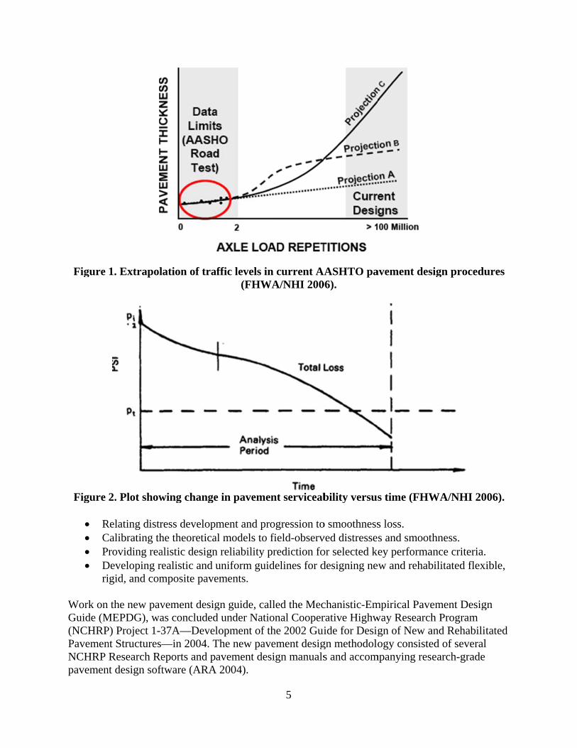
Step 1: Selection of Hierarchical Input Level for Each Input Parameter ................................. 11 Step 2: Develop Local Experimental Plan and Sampling Template ......................................... 12 Step 3: Estimate Sample Size for Specific Distress/IRI Prediction Models ............................. 12 Step 4: Select Pavement Projects .............................................................................................. 12 Step 5: Extract and Evaluate Distress and Project Data ........................................................... 13 Step 6: Conduct Field and Forensic Investigations ................................................................... 15 Step 7: Assess Local Bias—Validation of Global Calibration Values to Local Conditions, Policies, and Materials .............................................................................................................. 15 Step 8: Eliminate Local Bias of Distress and IRI Prediction Models ....................................... 17 Step 9: Assess the Standard Error of the Estimate .................................................................... 19 Step 10: Reduce Standard Error of the Estimate ...................................................................... 19 Step 11: Interpretation of Results, Deciding Adequacy of Calibration Parameters ................. 19

CHAPTER 3. DEVELOPMENT OF EXPERIMENTAL AND SAMPLING PLAN FOR COLORADO MEPDG MODELS VALIDATION/CALIBRATION .................................... 20

Select Hierarchical Input Level for Each Input Parameter ....................................................... 20 Develop Local Experimental Plan and Sampling Template ..................................................... 20 Identify Pavement Projects for Filling Sampling/Experimental Template ............................... 24 Estimate Sample Size for Specific Distress/IRI Prediction Models ......................................... 24

CHAPTER 4. PROJECTS SELECTION AND DEVELOPMENT OF CLIMATE AND TRAFFIC DATABASE TO VALIDATE/CALIBRATE MEPDG MODELS ...................... 27

Identification and Selection of Pavement Projects ................................................................... 27 Extracting, Assembling, and Evaluating Project Data (Project Database Development) ......... 48 Estimating Missing Data ........................................................................................................... 55

CHAPTER 5. DEVELOPMENT OF MATERIALS DATABASE FOR MEPDG MODEL VALIDATION/CALIBRATION ............................................................................................... 78

Construction Records and CDOT Pavement Projects QA/QC Data Review ........................... 79 Laboratory/Field Testing .......................................................................................................... 79 Laboratory Testing .................................................................................................................... 93

viii

CHAPTER 6. VERIFICATION AND CALIBRATION OF FLEXIBLE PAVEMENTS . 117

Alligator Cracking .................................................................................................................. 118 Total Rutting ........................................................................................................................... 125 Transverse “Thermal” Cracking ............................................................................................. 131 Smoothness ............................................................................................................................. 138 Estimating Design Reliability for New HMA and HMA Overlay Pavement Distress Models................................................................................................................................................. 142

CHAPTER 7. VERIFICATION AND CALIBRATION OF RIGID PAVEMENTS ......... 144

New JPCP and Unbonded JPCP Smoothness ......................................................................... 156 Estimating Design Reliability for New JPCP and Unbonded JPCP Overlay Distress Models................................................................................................................................................. 158

CHAPTER 8. INTERPRETATION OF RESULTS—DECIDING ADEQUACY OF CALIBRATION PARAMETERS ........................................................................................... 160

Verification of Colorado MEPDG Models (Sensitivity Analysis) ......................................... 160 Validation of Colorado MEPDG Models (Design Comparisons) .......................................... 172

CHAPTER 9. SUMMARY AND CONCLUSIONS ............................................................... 176

REFERENCES .......................................................................................................................... 177

APPENDIX A. NEW HMA AND NEW JPCP PERFORMANCE PREDICTION MODELS..................................................................................................................................................... A-1

New and Reconstructed HMA Pavements .............................................................................. A-1 New JPCP ............................................................................................................................... A-7

ix

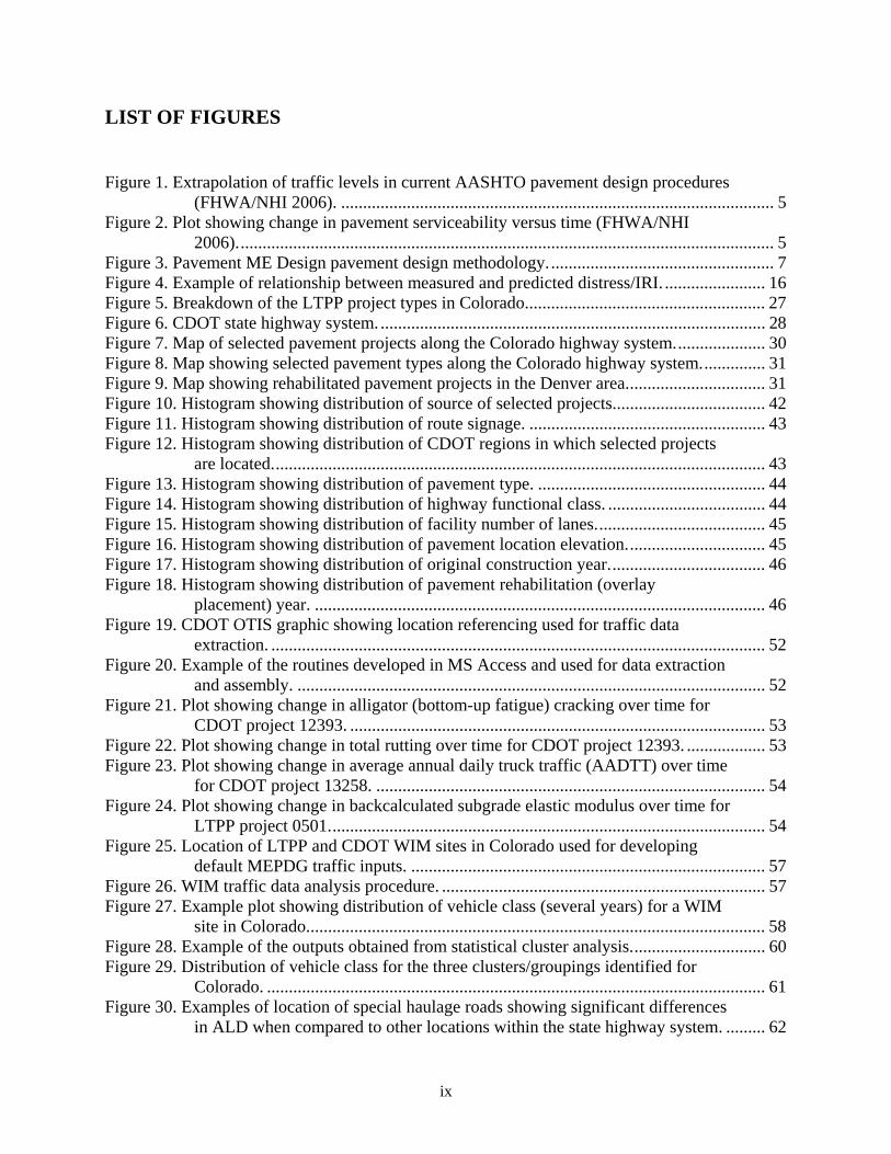
LIST OF FIGURES Figure 1. Extrapolation of traffic levels in current AASHTO pavement design procedures

(FHWA/NHI 2006). ................................................................................................... 5 Figure 2. Plot showing change in pavement serviceability versus time (FHWA/NHI

2006). .......................................................................................................................... 5 Figure 3. Pavement ME Design pavement design methodology. ................................................... 7 Figure 4. Example of relationship between measured and predicted distress/IRI. ....................... 16 Figure 5. Breakdown of the LTPP project types in Colorado. ...................................................... 27 Figure 6. CDOT state highway system. ........................................................................................ 28 Figure 7. Map of selected pavement projects along the Colorado highway system. .................... 30 Figure 8. Map showing selected pavement types along the Colorado highway system. .............. 31 Figure 9. Map showing rehabilitated pavement projects in the Denver area. ............................... 31 Figure 10. Histogram showing distribution of source of selected projects. .................................. 42 Figure 11. Histogram showing distribution of route signage. ...................................................... 43 Figure 12. Histogram showing distribution of CDOT regions in which selected projects

are located. ................................................................................................................ 43 Figure 13. Histogram showing distribution of pavement type. .................................................... 44 Figure 14. Histogram showing distribution of highway functional class. .................................... 44 Figure 15. Histogram showing distribution of facility number of lanes. ...................................... 45 Figure 16. Histogram showing distribution of pavement location elevation. ............................... 45 Figure 17. Histogram showing distribution of original construction year. ................................... 46 Figure 18. Histogram showing distribution of pavement rehabilitation (overlay

placement) year. ....................................................................................................... 46 Figure 19. CDOT OTIS graphic showing location referencing used for traffic data

extraction. ................................................................................................................. 52 Figure 20. Example of the routines developed in MS Access and used for data extraction

and assembly. ........................................................................................................... 52 Figure 21. Plot showing change in alligator (bottom-up fatigue) cracking over time for

CDOT project 12393. ............................................................................................... 53 Figure 22. Plot showing change in total rutting over time for CDOT project 12393. .................. 53 Figure 23. Plot showing change in average annual daily truck traffic (AADTT) over time

for CDOT project 13258. ......................................................................................... 54 Figure 24. Plot showing change in backcalculated subgrade elastic modulus over time for

LTPP project 0501. ................................................................................................... 54 Figure 25. Location of LTPP and CDOT WIM sites in Colorado used for developing

default MEPDG traffic inputs. ................................................................................. 57 Figure 26. WIM traffic data analysis procedure. .......................................................................... 57 Figure 27. Example plot showing distribution of vehicle class (several years) for a WIM

site in Colorado. ........................................................................................................ 58 Figure 28. Example of the outputs obtained from statistical cluster analysis. .............................. 60 Figure 29. Distribution of vehicle class for the three clusters/groupings identified for

Colorado. .................................................................................................................. 61 Figure 30. Examples of location of special haulage roads showing significant differences

in ALD when compared to other locations within the state highway system. ......... 62

x

Figure 31. Statewide and national ALD for single axles of class 5 and 9 trucks. ........................ 62 Figure 32. Statewide and national ALD for tandem axles of class 6 and 9. ................................. 63 Figure 33. CDOT statewide average, MEPDG, and Site 8-00008 ALD for tandem axles. ......... 63 Figure 34. Statewide and national ALD for tridem axles. ............................................................ 64 Figure 35. Statewide and national MEPDG averages for axle per trucks. ................................... 65 Figure 36. Statewide averages and default MAFs for class 5 and 9 trucks. ................................. 66 Figure 37. CDOT statewide averages and MEPDG default hourly truck volume

distribution. ............................................................................................................... 66 Figure 38. Locations of Colorado weather stations included in the MEPDG. ............................. 68 Figure 39. Locations of Colorado weather stations included in the MEPDG and NWS

cooperative stations. ................................................................................................. 69 Figure 40. Map showing location of MEPDG and CDOT weather stations. ............................... 71 Figure 41. Plot showing reported (blue dot) and estimated (red star) temperature data for

HCD file 31013 in Colorado. ................................................................................... 72 Figure 42. Plot showing reported (blue dot) and estimated (red star) wind speed data for

HCD file 31013 in Colorado. ................................................................................... 73 Figure 43. Plot showing reported (blue dot) and estimated (red star) percent cloud cover

data for HCD file 31013 in Colorado. ...................................................................... 74 Figure 44. Plot showing reported (blue dot) and estimated (red star) rainfall data for HCD

file 31013 in Colorado. ............................................................................................. 75 Figure 45. Plot showing reported (blue dot) and estimated (red star) relative humidity

data for HCD file 31013 in Colorado. ...................................................................... 76 Figure 46. Map of the locations of the 40 projects selected for field testing. ............................... 80 Figure 47. Schematic showing the outline of the field testing plan for each selected

project, along with coring patterns. .......................................................................... 80 Figure 48. Sampling section layout, core locations, and sample of extracted HMA core. ........... 82 Figure 49. Pavement coring rig used for materials extraction. ..................................................... 82 Figure 50. Example of field logging of extracted cores. ............................................................... 83 Figure 51. Distribution of as-placed HMA air voids estimated from field cores. ........................ 85 Figure 52. Distribution of as-placed volumetric binder content estimated from field cores. ....... 85 Figure 53. Sawing and lifting of surface HMA layer during the trenching operation. ................. 86 Figure 54. Lifting of the surface HMA layer during the trenching operation. ............................. 87 Figure 55. Inside of the completed trench (not the HMA and aggregate base layers). ................ 87 Figure 56. Plots of layer profile and rut depth across the 12-ft lane width. .................................. 88 Figure 57. Plots showing relationship between backcalculated k-value and MEPDG input

subgrade resilient modulus Mr at optimum moisture for month of FWD testing. ...................................................................................................................... 93

Figure 58. Comparison of HMA dynamic modulus E* for different binder grades. .................... 97 Figure 59. Comparison of HMA dynamic modulus E* for Superpave and SMA mixes. ............ 98 Figure 60. Comparison of HMA dynamic modulus E* for Level 1 and Level 3 estimates

(Mix FS-1938 (PG 64-22 & SX)). ............................................................................ 98 Figure 61. Comparison of HMA dynamic modulus E* for Level 1 and Level 3 estimates

(Mix FS-1918 (PG 58-28 & SX)). ............................................................................ 99 Figure 62. Comparison of HMA dynamic modulus E* for Level 1 and Level 3 estimates

(Mix FS-1939 (PG 76-28 & SX)). ............................................................................ 99

xi

Figure 63. Comparison of HMA dynamic modulus E* for Level 1 and Level 3 estimates (Mix FS-1919 (PG 76-28 & SMA)). ...................................................................... 100

Figure 64. Laboratory-measured creep compliance versus loading time. .................................. 103 Figure 65. Progression of HMA rutting with repeated load application obtained from

repeated load permanent deformation testing. ........................................................ 105 Figure 66. Example plot of permanent deformation vs. number of loading repetitions

obtained from HWT testing. ................................................................................... 106 Figure 67. Plot showing slope (m) and intercept (Is) computed from the secondary rutting

portion of plot of permanent strain vs. load repetitions. ......................................... 106 Figure 68. Plot of intercept (Is) vs. repeated load permanent deformation test temperature. ..... 107 Figure 69. Plot of compressive strength gain versus pavement age for CDOT PCC mixes....... 110 Figure 70. Plot of flexural strength gain versus pavement age for CDOT PCC mixes. ............. 111 Figure 71. Plot of laboratory-measured MR vs. CDOT statewide MR equation and

MEPDG global equation-predicted MR. ................................................................ 112 Figure 72. Plot of elastic modulus gain versus pavement age for CDOT PCC mixes. .............. 113 Figure 73. Plot of laboratory-measured EPCC vs. CDOT and MEPDG predicted EPCC. ........ 114 Figure 74. Example of distress map used for visual distress surveys. ........................................ 116 Figure 75. Verification of the HMA alligator cracking and fatigue damage models with

MEPDG global coefficients, using Colorado new HMA pavement projects only. ........................................................................................................................ 119

Figure 76. Plot showing predicted HMA alligator cracking versus computed fatigue damage developed using MEPDG models with CDOT local coefficients (for new HMA pavements only). ................................................................................... 122

Figure 77. Plot showing progression of reflection cracking with HMA overlay age for different HMA overlay thicknesses. ....................................................................... 123

Figure 78. Plot of predicted alligator cracking versus age for LTPP project 7783 (new HMA pavement). .................................................................................................... 123

Figure 79. Plot of predicted alligator cracking versus age for LTPP project 6002 (HMA overlaid HMA pavement). ...................................................................................... 124

Figure 80. Plot of predicted alligator cracking versus age for LTPP project 1029 (new HMA pavement). .................................................................................................... 124

Figure 81. Plot of predicted alligator cracking versus age for CDOT pavement management system project 13325. ....................................................................... 125

Figure 82. Plot showing MEPDG global model predicted rutting versus measured rutting (HMA, unbound aggregate base, and subgrade). ................................................... 126

Figure 83. Plot showing predicted using MEPDG submodels with CDOT local coefficients (for all pavements) versus field-measured total rutting. ..................... 129

Figure 84. Plot showing high variation of measured rutting over time for CDOT pavement management system project 13435. ....................................................... 129



Figure 87. Plot showing high variation of measured rutting over time for LTPP project 0503 (original construction). .................................................................................. 131

xii

Figure 88. Plot showing high variation of measured rutting over time for LTPP project 0503 (with HMA overlay). ..................................................................................... 131

Figure 89. Predicted versus measured transverse cracking using global coefficients and Colorado pavement sections with Level 1 inputs. .................................................. 133

Figure 90. Plot showing predicted versus measured transverse cracking developed using the MEPDG model with CDOT local coefficients and HMA transverse cracking distress from project field testing. ........................................................... 134

Figure 91. Plot showing predicted versus measured transverse cracking developed using MEPDG model with CDOT local coefficients and measured HMA transverse cracking distress. ................................................................................... 135

Figure 92. Plot showing predicted and measured transverse cracking versus pavement age for CDOT pavement management system project 13131. ..................................... 136






Figure 98. Predicted versus measured IRI using global MEPDG HMA IRI model and Colorado HMA pavement performance data. ........................................................ 139

Figure 99. Plot of measured and predicted IRI for new HMA and HMA-overlaid HMA pavements developed using the locally calibrated CDOT HMA IRI model. ......... 141

Figure 100. Plot showing measured and predicted IRI versus time for CDOT project 12448. ..................................................................................................................... 141



Figure 103. Histogram showing distribution of measured JPCP transverse “slab” cracking for CDOT and LTPP projects included in the analysis. ......................................... 146

Figure 104. Plot showing measured and predicted transverse “slab” cracking versus pavement age for JPCP projects using MEPDG global transverse cracking model coefficients. ................................................................................................. 147

Figure 105. Plot showing distribution of residuals (predicted – measured percent slab with transverse cracking) for all 246 observations included in the analysis. ......... 148

Figure 106. Plot of predicted and measured transverse cracking versus fatigue damage for LTPP 4_0213 (using global calibration factors and recommended loss of slab/aggregate base friction age). ........................................................................... 150

Figure 107. Plot of predicted and measured transverse cracking versus fatigue damage for LTPP 4_0217 (using global calibration factors and recommended loss of slab/lean concrete base friction age). ...................................................................... 150

xiii

Figure 108. Plot of predicted and measured transverse cracking versus fatigue damage for Colorado JPCP 54-11546 (using global calibration factors and recommended loss of slab/aggregate base friction age). ................................................................ 151

Figure 109. Histogram showing distribution of measured JPCP transverse joint faulting for CDOT pavement management system and LTPP projects included in the analysis. .................................................................................................................. 152

Figure 110. Plot showing distribution of residuals (predicted – measured faulting) for all 163 data points included in the analysis. ................................................................ 153

Figure 111. Predicted (using global calibration factors) and measured transverse joint faulting for Colorado JPCP 4_0213 (SPS-2) with dense graded aggregate base, dowel diameter = 1.5 in. ................................................................................ 154

Figure 112. Predicted (using global calibration factors) and measured transverse joint faulting for Colorado JPCP 4_0217 (SPS-2) with lean concrete base dowel diameter = 1.5 in. .................................................................................................... 155

Figure 113. Predicted (using global calibration factors) and measured transverse joint faulting for Colorado JPCP 4_0222 (SPS-2) with permeable asphalt treated base dowel diameter = 1.5 in. ................................................................................. 155

Figure 114. Predicted (using global calibration factors) and measured transverse joint faulting for Colorado JPCP 4_7776 (GPS-3) with dense graded aggregate base dowel diameter = 1.5 in. ................................................................................. 156

Figure 115. Predicted JPCP IRI versus measured Colorado JPCP with global calibration coefficients. ............................................................................................................ 156

Figure 116. Predicted and measured JPCP IRI for Colorado LTPP section 0216 over time. ........................................................................................................................ 157



Figure 119. Sensitivity summary for HMA pavement alligator cracking. Note the red line represents predicted alligator cracking for the baseline project in Table 75. ......... 162

Figure 120. Sensitivity summary for HMA pavement total (HMA, granular base, and subgrade) rutting. Note the red line represents predicted rut depth for the baseline project in Table 75. ................................................................................... 163

Figure 121. Sensitivity summary for HMA pavement transverse “thermal” cracking. Note the red line represents predicted transverse cracking for the baseline project in Table 75. ............................................................................................................. 164

Figure 122. Sensitivity summary for HMA pavement IRI. Note the red line represents predicted IRI for the baseline project in Table 75. ................................................. 165

Figure 123. Sensitivity summary for JPCP transverse “slab” cracking. Note the red line represents predicted percent slabs cracked for the baseline project in Table 76. ........................................................................................................................... 166

Figure 124. Sensitivity summary for JPCP transverse joint faulting. Note the red line represents predicted mean transverse joint faulting for the baseline project in Table 76. ................................................................................................................. 167

Figure 125. Sensitivity summary for JPCP IRI. Note the red line represents predicted IRI for the baseline project in Table 76. ....................................................................... 168

xiv

Figure 126. AASHTO 1993 HMA design thickness vs. AASHTO DARWin-ME HMA design thickness. ..................................................................................................... 173

Figure 127. AASHTO 1993 PCC design thickness vs. AASHTO DARWin-ME PCC design thickness ...................................................................................................... 175

xv

LIST OF TABLES Table 1. Summary of identified weaknesses in the 1961 through 1998 AASHTO

pavement design procedures (ARA 2004, FHWA/NHI 2006). ................................. 2 Table 2. Summary of distress/IRI thresholds (AASHTO 2008). .................................................. 14 Table 3. Process for minimizing bias in MEPDG predicted distress/IRI. .................................... 18 Table 4. Recommendations for modifying MEPDG flexible pavement distress/IRI models

global/local coefficients to eliminate bias. ............................................................... 18 Table 5. Recommendations for modifying MEPDG JPCP distress/IRI models global/local

coefficients to eliminate bias. ................................................................................... 18 Table 6. Summary of MEPDG global models statistics. .............................................................. 19 Table 7. Recommended hierarchical input levels for MEPDG models

validation/calibration in Colorado. ........................................................................... 21 Table 8. Sampling template for new HMA and HMA overlaid existing HMA pavements. ........ 23 Table 9. Sampling template for new JPCP, JPCP overlays of existing flexible pavements,

and unbonded JPCP of existing JPCP. ..................................................................... 24 Table 10. Description of Colorado environmental zone. .............................................................. 24 Table 11. Summary of distress/IRI thresholds and MEPDG nationally calibrated model

SEE (obtained from AASHTO 2008). ...................................................................... 25 Table 12. Minimum number of pavement projects required for the validation and local

calibration (AASHTO 2010). ................................................................................... 26 Table 13. Inventory information (highway type, route, & direction) for selected projects. ......... 32 Table 14. Inventory information (CDOT region, county, highway functional class, & no.

of lanes) for selected projects. .................................................................................. 35 Table 15. Inventory information (construction/rehab date, long/lat & elevation) for

selected projects. ....................................................................................................... 38 Table 16. Experimental template populated with new HMA and HMA-overlaid HMA

pavement projects for use in MEPDG flexible pavement model calibration/validation in Colorado. ........................................................................... 47

Table 17. Experimental template populated with new JPCP, JPCP overlays of flexible pavements, and unbonded JPCP of JPCP projects for use in MEPDG JPCP model calibration/validation in Colorado. ................................................................ 48

Table 18. LTPP sources of MEPDG input data for development of CDOT MEPDG calibration/validation database. ................................................................................ 49

Table 19. CDOT sources of MEPDG input data for development of CDOT MEPDG calibration/validation database. ................................................................................ 50

Table 20. Example of multiple project location references used for data extraction and assembly. .................................................................................................................. 51

Table 21. Summary of data availability for MEPDG models validation/calibration. .................. 56 Table 22. Examples of records availability for WIM/ATR sites in Colorado. ............................. 58 Table 23. Summary list of weather stations included in the MEPDG for Colorado. ................... 67 Table 24. Typical climate data ranges used in conducting QA/QC checks. ................................. 71 Table 25. Baseline time stamp for MEPDG HCD file development. ........................................... 71 Table 26. CDOT and MEPDG weather stations included in the MEPDG for Colorado.............. 77 Table 27. Summary of data availability for MEPDG models validation/calibration. .................. 78

xvi

Table 28. Summary of extracted HMA cores air voids and binder content test results. .............. 83 Table 29. Distribution of total rutting (percentage within layer) within the pavement

structure. ................................................................................................................... 88 Table 30. C1 values to convert calculated layer modulus values to an equivalent resilient

modulus measured in the laboratory. ........................................................................ 90 Table 31. Summary of HMA pavement backcalculated subgrade elastic modulus (ESG)

and subgrade lab Mr at optimum moisture content estimated from the backcalculated ESG.................................................................................................... 90

Table 32. Summary of rigid pavement backcalculated subgrade k-value and subgrade lab Mr at optimum moisture content estimated from the backcalculated subgrade k-value. ..................................................................................................................... 92

Table 33. CDOT mixes tested in the laboratory to develop MEPDG default inputs. ................... 94 Table 34. Volumetric properties and gradation of the selected typical CDOT HMA mixes. ....... 94 Table 35. Dynamic modulus values of typical CDOT HMA mixtures. ....................................... 95 Table 36. HMA dynamic modulus master curve parameters for typical CDOT HMA

mixtures. ................................................................................................................... 97 Table 37. Creep compliance values of typical CDOT HMA mixtures. ...................................... 101 Table 38. Indirect tensile strength values of typical CDOT HMA mixtures. ............................. 102 Table 39. Statistical comparison of Level 1 laboratory-tested and Level 3 MEPDG

computed creep compliance for the selected CDOT HMA mixtures. .................... 103 Table 40. Statistical comparison of Level 1 laboratory-tested and Level 3 MEPDG

computed indirect tensile strength for the selected CDOT HMA mixtures. .......... 104 Table 41. Estimates of HMA rutting model k1, k2, and k3 parameters for the selected

CDOT HMA mixtures using the repeated load permanent deformation test procedure (Von Quintus et al. 2012). ..................................................................... 107

Table 42. Estimates of HMA rutting model k1, k2, and k3 parameters for the selected CDOT HMA mixtures using the HWT test procedure. .......................................... 108

Table 43. Properties of typical CDOT PCC mixtures. ................................................................ 109 Table 44. Materials and sources used in typical CDOT PCC mixtures. ..................................... 109 Table 45. Compressive strength of typical CDOT PCC mixtures. ............................................. 110 Table 46. Flexural strength of typical CDOT PCC mixtures. ..................................................... 111 Table 47. Static elastic modulus and Poisson’s ratio of typical CDOT PCC mixtures. ............. 113 Table 48. CTE values of typical CDOT PCC mixtures. ............................................................. 115 Table 49. Criteria for determining global models adequacy for Colorado conditions. .............. 117 Table 50. MEPDG flexible pavement global models evaluated for Colorado local

conditions. .............................................................................................................. 118 Table 51. Results of statistical goodness of fit and bias evaluation of the MEPDG

alligator cracking global model for Colorado conditions. ...................................... 119 Table 52. Description of HMA fatigue damage, HMA alligator cracking, and reflection

“alligator” cracking models. ................................................................................... 120 Table 53. Summary of MEPDG global and CDOT local calibration coefficients for HMA

alligator cracking and HMA fatigue damage models. ............................................ 121 Table 54. Results of statistical evaluation of MEPDG alligator cracking and fatigue

damage local models for Colorado conditions. ...................................................... 121 Table 55. Local calibration coefficients for HMA overlay reflection cracking model

developed using new HMA and HMA overlaid HMA pavement projects. ........... 121

xvii

Table 56. Results of statistical bias evaluation of MEPDG reflection “alligator” cracking local model for Colorado conditions. ..................................................................... 121

Table 57. Results of statistical evaluation of MEPDG total rutting global submodels for Colorado conditions. ............................................................................................... 126

Table 58. Description of total rutting prediction submodels. ..................................................... 127 Table 59. Local calibration coefficients for HMA, unbound base, and subgrade soil

rutting submodels. .................................................................................................. 128 Table 60. Results of statistical evaluation of MEPDG alligator cracking and fatigue

damage local models for Colorado conditions. ...................................................... 129 Table 61. Colorado environmental zones. .................................................................................. 132 Table 62. Results of statistical evaluation of MEPDG transverse cracking global model

for Colorado conditions. ......................................................................................... 133 Table 63. Local calibration coefficients for transverse cracking. ............................................... 134 Table 64. Results of statistical evaluation of MEPDG transverse cracking local model for

Colorado conditions. ............................................................................................... 135 Table 65. Results of statistical evaluation of MEPDG transverse cracking local model for

Colorado conditions using measured HMA transverse cracking data. ................... 135 Table 66. Results of statistical evaluation of MEPDG HMA IRI global model for

Colorado conditions. ............................................................................................... 139 Table 67. Local calibration coefficients for HMA smoothness (IRI) model. ............................. 140 Table 68. Results of statistical evaluation of MEPDG HMA IRI local model for Colorado

conditions. .............................................................................................................. 140 Table 69. Criteria for determining global models adequacy for Colorado conditions. .............. 144 Table 70. MEPDG rigid pavement global models evaluated for Colorado local

conditions. .............................................................................................................. 145 Table 71. Comparison of measured and predicted transverse cracking (percentage of all

measurements). ....................................................................................................... 147 Table 72. Frequency distributions of measured transverse cracking data. ................................. 149 Table 73. Comparison of measured and predicted transverse joint faulting (percentage of

all measurements). .................................................................................................. 152 Table 74. Goodness of fit and bias test statistics for final Colorado calibrated JPCP IRI

model (based on 100 percent of all selected projects). ........................................... 157 Table 75. Mean (baseline) and range of key inputs used for sensitivity analysis of new

HMA pavements. .................................................................................................... 161 Table 76. Mean (baseline) and range of key inputs used for sensitivity analysis of new

JPCP. ...................................................................................................................... 161 Table 77. Summary of sensitivity analysis of new HMA pavements results. ............................ 171 Table 78. Summary of sensitivity analysis of new JPCP results. ............................................... 171 Table 79. Description of key inputs used for design comparisons. ............................................ 172 Table 80. Summary of the results from the new HMA design projects. .................................... 173 Table 81. New HMA pavement goodness of fit and bias test for final local CDOT

MEPDG and 1993/1998 AASHTO Pavement Design Guide design thicknesses. ............................................................................................................. 174

Table 82. Summary of the results from the new JPCP design projects. ..................................... 175 Table 83. New JPCP goodness of fit and bias test for final local CDOT MEPDG and

1993/1998 AASHTO Pavement Design Guide design thicknesses. ...................... 175

xviii

LIST OF ABBREVIATIONS AADTT Average annual daily truck traffic AASHTO American Association of State Highway and Transportation Officials AC Asphalt concrete ALD Axle load distribution ATB Asphalt treated base ATLAS Advanced Traffic Loading Analysis System ATR Automated traffic recorder CAPA Colorado Asphalt Pavement Association CCC Cubic clustering criterion CDOT Colorado Department of Transportation CPR Concrete pavement restoration CRCP Continuously reinforced concrete pavement CTB Cement treated base CTE Coefficient of thermal expansion DGAB Dense graded asphalt base ESAL Equivalent single axle load FHWA Federal Highway Administration FWD Falling Weight Deflectometer HMA Hot-mix asphalt HWT Hamburg Wheel Tracking IDT Indirect tensile IRI International Roughness Index JPCP Jointed plain concrete pavement JTCP Joint Technical Committee on Pavements LCB Lean concrete base LTPP Long Term Pavement Performance MAF Monthly adjustment factor MEPDG Mechanistic-Empirical Pavement Design Guide NCDC National Climatic Data Center NCHRP National Cooperative Highway Research Program NRCS National Resources Conservation Service NWS National Weather Service OTIS Online Transportation Information System PATB Permeable asphalt treated base PCC Portland cement concrete PMA Polymer modified asphalt PSF Pseudo F PSI Present serviceability index PST2 Pseudo t2 QA Quality assurance QC Quality control R2 Coefficient of determination RLPD Repeated load permanent deformation

xix

SEE Standard error of estimate SMA Stone matrix asphalt SSURGO Soil Survey Geographic (database) USDA United States Department of Agriculture VAR Variance Vbeff Volumetric moisture content VFA Voids filled with asphalt VMA Voids in mineral aggregate WIM Weigh-in-motion

1

CHAPTER 1. INTRODUCTION Background For many years, the Colorado Department of Transportation (CDOT) has used the 1993 American Association of State Highway and Transportation Officials (AASHTO) Guide for Design of Pavement Structures and the 1998 supplement to design new and rehabilitated flexible and rigid pavements (AASHTO 1993, AASHTO 1998). The 1993 AASHTO Pavement Design Guide originated from empirical pavement design equations developed in the late 1950s using pavement performance data collected under a national research program known as the AASHO Road Test (HRB 1962). Over the years, several editions of the AASHTO design guide have been published (AASHTO 1961, AASHTO 1972, AASHTO 1986, AASHTO 1993, AASHTO 1998). The original empirical pavement design equations were improved over the years to address, as much as possible, identified weaknesses in the design procedure. Table 1 summarizes these identified weaknesses, such as (1) the absence of sophisticated materials and traffic loading characterizations algorithms and (2) the lack of algorithms that relate applied truck axle load with pavement mechanical responses that lead to the development and progression of damage, distresses, and smoothness loss. Although these design guides have served as the primary tool for pavement design in the U.S. and beyond for many decades, and they have been used successfully to design many types of pavements, the inherent weaknesses of the design procedure have resulted in designs of many pavement structures that have under-performed or have failed prematurely. In 1996, the AASHTO Joint Technical Committee on Pavements (JTCP) proposed a shift from empirical-based to mechanistic-based pavement design. This was to be done through the development of a new pavement design guide based on mechanistic principles for the design of new and rehabilitated pavement structures. Key aspects of mechanistic principles to be included in the new pavement design technology included (ARA 2004):

Mechanistically characterizing paving materials properties (asphalt concrete, portland cement concrete, chemically stabilized unbound granular and soil materials) accurately and in real time.

Simulating ambient temperature and moisture conditions and their interaction with pavement material properties.

Simulating truck traffic loading and forecasting growth.Mechanistically calculating pavement response (i.e., stresses, strains, and deflections) due to traffic loadings for various environmental conditions.

Relating pavement response to incremental damage and deterioration. Accumulating incremental pavement damage over time and relating accumulated

pavement damage empirically to distress development and progression (cracking, rutting, faulting, punchouts, etc.).

2

Table 1. Summary of identified weaknesses in the 1961 through 1998 AASHTO pavement design procedures (ARA 2004, FHWA/NHI 2006).

Identified Weakness Description & Remedial Action

Traffic characterization

(1) Description: a. Equivalent 18-kip single axle load (ESAL) was used to characterize the traffic loading. It is doubtful that the equivalency factors

developed at the AASHO Road Test are applicable to today’s traffic stream (combination of axle load levels and types of axles). b. Heavy truck traffic levels have increased tremendously since the 1960s. Interstate pavements were designed in the 1960s for 5 to

10 million ESALs, while the AASHO Road Test pavements carried approximately 1 million axle load applications. Today, interstate pavements are designed for 50 to 200 million axle loads or more. Thus, it is not realistic to expect the original empirical pavement design models to design for today’s level of traffic without extrapolating the design methodology far beyond the original traffic inference space. Highly trafficked projects are thus likely to be under- or over-designed (see Figure 1)

(2) Remedial action: None

Design

(1) Description: a. Shoulder type/edge support for rigid pavements: Gravel shoulders were used at the AASHO Road Test, so full-width paving

effects are not adequately considered. b. Pavement subdrainage: Original flexible pavements were built in a “bathtub,” resulting in a very poor subdrainage condition that

was reflected in the pavement design models. c. Joint deterioration: For jointed rigid pavements, joint deterioration (characterized mostly in terms of load transfer efficiency

(LTE)) and its impact on future pavement performance was not directly considered d. Rehabilitation: The AASHO Road Test included only new flexible and rigid pavements. Rehabilitated pavement was not

considered. (2) Remedial action:

a. The 1986 Pavement Design Guide introduced guidance for the design of subsurface drainage systems and modified the flexible and rigid pavement design equations to take advantage of improvements in performance due to good drainage. The benefits of drainage were incorporated into the structural number via the empirical drainage coefficients m and Cd.

b. The 1986 Pavement Design Guide introduced a methodology for assessing the effects of environment on pavement performance. Specific emphasis is given to frost heave, thaw-weakening, and swelling of subgrade soils.

c. The 1986 Pavement Design Guide introduced the J-factor representing joint load transfer. d. The 1993 Pavement Design Guide included a methodology for rehabilitation designs for flexible and rigid pavement systems

using overlays. e. The 1998 supplement to the 1993 Pavement Design Guide provided an improved method for rigid pavement design.

3

Table 1. Summary of identified weaknesses in the 1961 through 1998 AASHTO pavement design procedures, continued (ARA 2004, FHWA/NHI 2006).

Identified Weakness

Description & Remedial Action

Materials characterization

(1) Description: a. Asphalt concrete: New, improved asphalt mixtures such as SuperPave, stone matrix asphalt, polymer-modified asphalt, etc., are

not directly incorporated into the empirical design model. b. Base/subbase layers: A dense crushed unbound limestone aggregate base was used at the AASHO Road Test. The subbase layer

was uncrushed and unbound gravel/sand. The unbound aggregate base/subbase produced a generally impervious granular “bathtub” that experienced significant loss of support during spring thaw, resulting in greater deterioration rates than typical.

c. Durability: There were few material durability problems (such as asphalt stripping and corrosion of steel in concrete) over the 2-year AASHO Road Test period. Thus, the effect of long-term material durability on performance was not considered.

(2) Remedial action: a. The 1972 Pavement Design Guide presented guidance for estimating structural layer coefficients a1, a2, and a3 for materials

other than those at the AASHO Road Test. These guidelines were based primarily on a survey of state highway agencies regarding the values for the layer coefficients that they were currently using in design for various materials. The 1972 Pavement Design Guide recommends that, “because of widely varying environments, traffic, and construction practices, it is suggested that each design agency establish layer coefficients applicable to its own experience.”

b. The 1986 Pavement Design Guide introduced the resilient modulus for determining the structural layer coefficients for both stabilized and unstabilized unbound materials in flexible pavements.

Foundation characterization

(1) Description: Pavements at the AASHO Road Test site were constructed over a single silty-clay (AASHTO A-6) subgrade. The effect of this single subgrade was “built into” the empirical design models.

(2) Remedial action: a. The 1972 Pavement Design Guide included an empirical soil support scale to reflect the influence of local foundation soil

conditions for flexible pavements. This scale ranged from 1 to 10, with a soil support value Si of 3 corresponding to the silty clay foundation soils at the AASHO Road Test site and the upper value of 10 corresponding to crushed rock base materials. All other points on the scale were assumed from experience, with some limited checking through theoretical computations.

b. For rigid pavements, the use of the Spangler/Westergaard theory for stress distributions in rigid slabs to incorporate the effects of local foundation soil conditions was added to the 1972 Pavement Design Guide to extend the rigid pavement design methodology to soil conditions other than those at the AASHO Road Test. Foundation soil conditions were characterized by the overall modulus of subgrade reaction, k, which is a measure of the stiffness of the foundation soil.

c. The 1986 Pavement Design Guide introduced the use of the resilient modulus, Mr, as a stiffness parameter for characterizing the soil support provided by the subgrade. Mr is a measure of the resilient modulus of the soil recognizing certain nonlinear characteristics.

d. The 1986 Pavement Design Guide introduced the use of nondestructive deflection testing for evaluating existing pavement and backcalculation of layer moduli.

4

Table 1. Summary of identified weaknesses in the 1961 through 1998 AASHTO pavement design procedures, continued (ARA 2004, FHWA/NHI 2006).

Identified Weakness

Description & Remedial Action

Empirical nature of pavement design equations

(1) Description: A combination of graphical techniques and least squares regression was used to develop the empirical pavement equations using approximately 2 years of pavement performance data. The original models have been “extended” over time based on empirical concepts, most of which have not been verified with field data. The procedure cannot solve for the required thickness of hot-mix asphalt (HMA), only structural number, which can lead to serious design deficiencies.


Functional form of empirical pavement models

(1) Description: The form of the mathematical models used to fit the performance data collected at the AASHO Road Test (i.e., 2 years of gradually sloping downward serviceability trends) does not appear to fit the shape of the long-term performance trends of many in-service pavements that have demonstrated the opposite shape (i.e., they show more rapid loss of serviceability in the initial years, before leveling off)—see Figure 2.


Climate

(1) Description: The pavement design models were developed over a 2-year period at the AASHO Road Test site in northern Illinois; thus, they have been calibrated for just one climatic condition and 2 years of climatic cycles, both of which are serious limitations of the procedure.

(2) Remedial action: a. In 1972, an empirical regional factor, R, was introduced to provide an adjustment to the flexible pavement structural number for

local environmental and other considerations. Values for the regional factor were estimated from serviceability reduction rates in the AASHO Road Test. These estimates varied between 0.1 and 4.8, with an annual average value of about 1.0. The regional factor was not recommended for special conditions, such as serious frost conditions, or other local problems.

b. The ability to adjust for other climates was included in the original models through the addition of a drainage coefficient in 1986. The drainage coefficient, however, includes only a portion of the effect of climate (i.e., moisture, not temperature or freeze-thaw cycles). Highways loaded in other climates would have different rates of deterioration.

Figure

Figure

R C P D

ri Work onGuide (M(NCHRPPavemenNCHRP pavemen

1. Extrapol

2. Plot show

Relating distrCalibrating th

roviding reaDeveloping reigid, and com

the new pavMEPDG), waP) Project 1-3nt Structures—Research Re

nt design soft

lation of tra

wing change

ress developmhe theoreticaalistic designealistic and umposite pave

vement desigas concluded37A—Devel—in 2004. Teports and p

ftware (ARA

affic levels in(FHW

e in paveme

ment and pral models to n reliability puniform guidements.

gn guide, cald under Natiolopment of tThe new pavavement des

A 2004).

5

n current AWA/NHI 200

ent serviceab

ogression tofield-observprediction fodelines for d

lled the Meconal Cooperthe 2002 Guivement desigsign manuals

AASHTO pa06).

bility versus

o smoothnessved distresseor selected kedesigning ne

chanistic-Emrative Highwide for Desig

gn methodolos and accom

avement des

s time (FHW

s loss. s and smootey performa

ew and rehab

mpirical Paveway Researchgn of New aogy consiste

mpanying res

sign procedu

WA/NHI 20

thness. ance criteria.bilitated flex

ement Desigh Program and Rehabilited of severalearch-grade

ures

006).

ible,

gn

tated l

6

The 2004 version of the MEPDG has undergone several independent reviews and refinements since initial completion. AASHTO adopted the revised MEPDG in 2007 as an interim standard for pavement design in the U.S. The following professional versions of the research products have since been developed (AASHTO 2008, AASHTO 2013):

Mechanistic-Empirical Pavement Design Guide, Interim Edition: A Manual of Practice. AASHTOWare Pavement ME Design.

Pavement ME Design uses state-of-the-practice mechanistic-based pavement analysis and distress prediction algorithms. The distress prediction models were calibrated using field-observed distress and International Roughness Index (IRI) data from several hundred experimental flexible, rigid, and composite in-service pavements located throughout the U.S. as part of the Federal Highway Administration (FHWA) Long Term Pavement Performance (LTPP) database and other national databases (e.g., MnROAD). These models are hence termed “global” calibrated models. Overview of the AASHTO’s Pavement ME Design Pavement ME Design can be used to design or perform forensic analysis of 17 new and rehabilitated pavement types, namely (AASHTO 2008):

New or reconstructed HMA pavement. New or reconstructed jointed plain concrete pavement (JPCP) and continuously

reinforced concrete pavement (CRCP). Rehabilitation with HMA—HMA overlay on existing HMA, JPCP, or CRCP. Rehabilitation with portland cement concrete (PCC)—Bonded or unbonded JPCP

overlay of existing JPCP, CRCP, and flexible pavement. Rehabilitation with PCC—Bonded or unbonded CRCP overlay of existing JPCP or

CRCP. Rehabilitation with PCC—JPCP or CRCP overlay of existing HMA. JPCP rehabilitation—Concrete pavement restoration (CPR) and diamond grinding.

The Pavement ME Design approach is presented in Figure 3.

7

Figure 3. Pavement ME Design pavement design methodology.

Foundation Analysis

REHABILITATIONEvaluate Existing

Pavement

DrainageVolume Changes

Frost Heave

NEW PAVEMENTSSubgrade Analysis

ENVIRONMENTTemperature

Moisture

PAVEMENT MATERIALSProperties as functions of loading

rate, temperature, & moisture

TRAFFICAxle Loads

ClassificationForecasting

RELIABILITY

Modify StrategySelect Trial

Pavement Strategies

Pavement Response Models

Pavement PerformanceModels

Doesperformance

meetcriteria?

EngineeringAnalysis

ViableAlternatives

Life CycleCost Analysis

SelectStrategy

STAGE 1 -- EVALUATION

STAGE 2 -- ANALYSIS

STAGE 3 – STRATEGY SELECTION

No

Yes

Other Considerations

Foundation Analysis

REHABILITATIONEvaluate Existing

Pavement

DrainageVolume Changes

Frost Heave

NEW PAVEMENTSSubgrade Analysis

ENVIRONMENTTemperature

Moisture

PAVEMENT MATERIALSProperties as functions of loading

rate, temperature, & moisture

TRAFFICAxle Loads

ClassificationForecasting

RELIABILITY

Modify StrategySelect Trial

Pavement Strategies

Pavement Response Models

Pavement PerformanceModels

Doesperformance

meetcriteria?

EngineeringAnalysis

ViableAlternatives

Life CycleCost Analysis

SelectStrategy

STAGE 1 -- EVALUATION

STAGE 2 -- ANALYSIS

STAGE 3 – STRATEGY SELECTION

No

Yes

Other Considerations

8

The Pavement ME Design approach involves the following (AASHTO 2008):

Development of input values. For the analysis, establishment of performance criteria (not-to-exceed distress thresholds) and associated design reliability levels for each criterion.

Structural/performance analysis. The analysis approach is an iterative one that begins with the selection of an initial trial design. The trial section is analyzed incrementally over time using the pavement response and distress models, and the outputs of the analysis are accumulated damage (the expected amount of distress and smoothness over time). If the trial design does not meet the performance criteria, modifications are made and the analysis re-run until a satisfactory result is obtained. An optimization routine is available to solve for adequate thickness of the HMA and PCC layers and other factors.

Activities required for evaluating structurally viable design alternatives. These activities include an engineering analysis and life cycle cost analysis of the alternatives.

Pavement ME Design provides a uniform and comprehensive set of procedures for the design of new and rehabilitated flexible and rigid pavements. It employs common design parameters for traffic, subgrade, climate, and reliability for all pavement types. Recommendations are provided for the structure (layer materials and thickness) of new and rehabilitated pavements, including procedures to select pavement layer thickness, rehabilitation treatments, subsurface drainage, foundation improvement strategies, and other design features. The procedures can be used to develop alternate designs using a variety of materials and construction procedures. The benefits of Pavement ME Design are many, and they will impact all levels of pavement operation, from planning through design and construction, to ongoing maintenance and rehabilitation, to eventual reconstruction. The major benefits are summarized as follows (AASHTO 2008):

Ability to assess the impact of new and innovative pavement materials (asphalt binders, recycled aggregates, etc.) on pavement performance.

Ability to assess the impact of aging and long-term durability of materials on performance.

Distress/IRI prediction models far superior to current empirical serviceability prediction models.

Design reliability approach is sound at low and high traffic levels. More cost-effective designs (through better handling of reliability and better handling

of the interactions between materials and site factors). Fewer premature pavement failures caused by deficient design and materials (the

MEPDG allows the user to analyze “what if” scenarios to quantify the impact of design assumptions of pavement life).

Less likelihood of very thick over-design for heavy traffic (currently caused by deficient empirical equations based on a few million trucks at the AASHO Road Test).

Improved tool for innovative contracting, assessing effects of substandard quality of construction, etc.

9

Improved tool for highway cost allocation studies, pavement management, etc. Improved tool for specialized designs (impacts of special truck loadings, cold

temperatures, high groundwater table, etc.). MEPDG Implementation in Colorado CDOT has been preparing for the implementation of the MEPDG since 2001, when CDOT and the Colorado Asphalt Pavement Association (CAPA) initiated a project to develop a road map for implementing the MEPDG flexible pavement design and analysis procedure in Colorado. The road map was developed from a series of facilitated meetings between CDOT, CAPA, and industry representatives. An analogous rigid pavement design road map also was also developed in 2001. These road maps were updated and refined in 2007 and served as a guide for implementing version 1.0 of the MEPDG. Objective of Study The objective of this study is to provide all information and documents necessary for CDOT and industry to use the latest MEPDG software (Pavement ME Design) on a day-to-day basis for the design and analysis of new and rehabilitated pavement structures in Colorado. Scope of Study The following activities and products were developed during the course of the project to achieve the study objective:

1. Identify resources needed to implement the MEPDG. 2. Validate and calibrate version 1.0 of the MEPDG specific to Colorado site conditions,

materials, and typical design features used to construct new pavements and rehabilitate existing pavements.

a. Confirm or adjust input default values for Colorado conditions. b. Confirm or adjust the calibration coefficients to avoid biased designs. c. Recommend any changes in policy and procedure that will be needed.

3. Prepare a design manual and other documents to establish consistent use of the MEPDG and resulting designs.

4. Recommend design reliability levels and performance criteria levels for design of various highway classes.

5. Establish traffic and materials libraries that are representative of the truck traffic and paving materials found in Colorado. These libraries will facilitate the use of consistent inputs and provide ease of use by importing specific inputs into the MEPDG that are representative of Colorado roadways.

6. Provide training on the use of the verified and calibrated MEDPG, along with training materials that CDOT can continue to use and update for future reference.

10

Organization of Report This report documents work done under this project, specifically the tasks listed below, that resulted in implementation of the MEPDG in Colorado:

Task 0 – Project kick-off meeting and coordination task. Task 1 – Database development. Task 2 – Field investigations and laboratory materials testing. Task 3 – Verification of current MEPDG. Task 4 – Local calibration and validation of performance models. Task 5 – Development of CDOT MEPDG design manual. Task 6 – Deployment of concurrent designs during transition to MEPDG method. Task 7 – Development of default input libraries. Task 8 – Training program delivery. Task 9 – Preparation and submittal of the draft final and final reports.

Chapter 2 describes the framework utilized for MEPDG global models validation and local calibration (if needed) for Colorado conditions. The framework was adapted after the guidelines presented in the AASHTO Guide for the Local Calibration of the Mechanistic-Empirical Pavement Design Guide (AASHTO 2010). Chapter 3 describes the development of experimental and sampling plan for Colorado MEPDG models validation/calibration, while chapter 4 describes project selection and development of the validation/calibration database. Chapter 4 also provides a full and detailed description of CDOT traffic, climate, and materials test data used to develop default libraries, along with records review, data assembly and cleansing, and laboratory/field testing done as part of the database development effort. Chapter 5 presents a detailed description of the statistical analysis performed to validate and calibrate the MEPDG models and design procedure for Colorado conditions. Chapter 6 presents work done to validate the new local MEPDG models and design procedure for Colorado (sensitivity analysis and design comparisons). Chapter 7 summarizes the work done under this project and the outcomes. Recommendations for future work are also presented in this chapter. Appendix A presents details of the MEPDG distress and IRI models for the pavement types of relevance to this project.

11

CHAPTER 2. FRAMEWORK FOR LOCAL CALIBRATION OF THE MEPDG IN COLORADO This chapter presents a framework for local calibration of the MEPDG. It is adapted after the AASHTO Guide for the Local Calibration of the Mechanistic-Empirical Pavement Design Guide (AASHTO 2010). In all, model validation and local calibration consists of the 11 steps described in this chapter. Step 1: Selection of Hierarchical Input Level for Each Input Parameter The AASHTO MEPDG Manual of Practice describes hierarchical input levels as follows (AASHTO 2008):

Level 1 inputs provide for the highest level of accuracy and, thus, would have the lowest level of uncertainty or error. Level 1 material inputs require laboratory or field testing, such as the dynamic modulus testing of HMA, site-specific axle load spectra data collections, or nondestructive deflection testing.

Level 2 inputs provide an intermediate level of accuracy and would be closest to the typical procedures used with earlier editions of the AASHTO Pavement Design Guide. Level 2 inputs typically would be user-selected, possibly from an agency database, could be derived from a limited testing program, or could be estimated through correlations such as using R-value to estimate resilient modulus.

Level 3 inputs provide the lowest level of accuracy. Inputs typically would be user-selected values based on national averages, engineering experience, or typical averages of an input for the region or state.

For MEPDG model validation and local calibration, the AASHTO local calibration guide recommends selecting an appropriate mix of MEPDG hierarchical input levels (1 through 3) consistent with the agency’s day-to-day practices for characterizing pavement inputs for design. If good Level 3 and Level 2 procedures and recommendations are developed during local calibration, these inputs should provide reasonable designs. Of course, the more Level 1 inputs, the better. In addition, inputs found to have a major impact on MEPDG distress/IRI predictions must be characterized as accurately as possible using the highest possible hierarchical input level. This is because the mix of hierarchical input levels used for models calibration ultimately has a major impact on predicted distress/IRI standard error or deviation. Predicted distress/IRI standard error is a key component of the variability terms used in calculating design reliability. The models’ standard error was derived using inputs derived from all three levels; however, there was a considerable proportion of Level 1 and 2 inputs for all of the projects used in calibration.

12

Step 2: Develop Local Experimental Plan and Sampling Template A detailed, statistically sound experimental plan/sampling template is required for use in identifying and selecting Colorado pavement projects for use in MEPDG model validation and local calibration. The experimental plan was designed to ensure the following:

Determine bias in MEPDG distress/IRI predictions (using national coefficients). Establish cause of bias, if present. Determine local calibration coefficients for each distress/IRI model with identified bias.

The new model local calibration coefficients must be established to reduce bias and maximize accuracy.

A key aspect of the experimental/sampling template was to ensure that it could be used to obtain a mix of pavement projects that reflect current and future CDOT pavement types, design features, material types, and site conditions. Key factors used in defining the sampling template are:

Pavement type. Surface layer thickness. Climate zone. Base and subgrade type. Asphalt concrete (AC) mix binder type. Rigid pavement design features (load transfer mechanism, edge support, etc.). Truck traffic applications level.

Once the sampling template was defined, attempts were made to obtain an adequate number of pavement projects to populate each cell within the sampling template (i.e., a full factorial balanced factorial with replicate pavement projects within each populated cell). Where this was not possible, a fractional balanced factorial was adopted and used, as it was too costly to fully populate all cells with projects. Step 3: Estimate Sample Size for Specific Distress/IRI Prediction Models Under this step the minimum number of projects required to validate/calibrate the MEPDG global models was determined. The minimum sample size in theory was to be determined separately for each distress/IRI prediction model. However, in practice the maximum number of projects required for each pavement type is adopted. The AASHTO Guide for the Local Calibration of the MEPDG provides recommendations for determining sample size and this was adopted for this project. Step 4: Select Pavement Projects Once the required minimum number of projects for local calibration/validation is determined the next step is to identify local projects to populate the sampling template. Potential of sources of pavement projects are presented as follows:

13

National and local research/experimental test pavements. Pavement management sections in general.

The candidate projects must be reviewed for selection based on criteria described in steps 1 through 3, including:

Historical distress/IRI of selected projects should cover the reasonable range of values typical for Colorado (including the threshold values).

As much as possible, they must be representative of current and future CDOT pavement design and construction practices.

They must be representative of Colorado site (traffic, climate, and subgrade) conditions. In general, the selected projects must have the fewest number of structural layers. For rehabilitated pavements, projects with detailed historical distress/IRI data before and after rehabilitation must be given a higher priority. Projects with unconventional designs and material types must be selected only if they represent anticipated future designs. Step 5: Extract and Evaluate Distress and Project Data This step involves the following four activities:

1. Extract, review, and convert historical measured distress/IRI data for each identified project into the units predicted by the MEPDG. This involves assembling relevant historical measured distress and smoothness data for the selected projects from agency pavement management system data tables, research reports, research-type experimental projects databases, and so on. The assembled data are then reviewed for accuracy, reasonableness, and consistency. As needed, the raw distress/IRI data as measured and reported are converted into the MEPDG reporting units for each performance indicator. Note that the MEPDG distress and smoothness predictions are defined according the LTPP Distress Identification Manual (Miller & Bellinger 2003).

2. Compare performance indicator magnitudes to the design threshold values (see Table 2). a. This involves a comparison of the magnitudes of the design threshold values and

historical distress/IRI measurements from the selected projects. The goal is to determine whether measured distress/IRI to be used in calibration/validation cover the agency’s design threshold values. Using projects with historical measured distress/IRI values close to the design threshold values ensures that the models are calibrated/validated to predict distress/IRI accurately within the range of distress/IRI of greatest importance to the agency.

b. Each project was assigned the same weight during statistical analysis (calibration/validation). Assigning the same weight implies that repeated distress/IRI measures of each project will be approximately the same. A key step is to determine the number of distress/IRI records available for each selected project. Once this is done, possible significant differences in the number of records available must be noted for corrective action to be taken as part of statistical analysis.

14

3. Evaluate the distress data to identify anomalies and outliers. Bivariate plots of distress and IRI versus pavement age must be developed for each project and distress/IRI performance indicator. Each plot is then reviewed and evaluated. The review is limited to visual inspection of time series plots showing the progression of distress and IRI to (1) determine if observed trends in distress/IRI progression are reasonable, (2) identify potential anomalies (e.g., significant decrease in distress/IRI magnitude indicating an occurrence of significant rehabilitation or maintenance event), and (3) identify potential outliers. The results of this exercise serve to:

a. Identify projects exhibiting unreasonable trends in distress/IRI progression and correct the anomalies identified, if possible. Otherwise, the project is removed from the project database for the given anomalous performance indicator. It must be noted that each distress type and IRI were treated separately; thus, removal of a project from, say, the rutting database does not imply that it was also removed from the transverse cracking database.

b. Individual distress/IRI observations identified as outliers or erroneous are removed. Examples include zero measurements that could represent non-entry values and significantly high or low distress/IRI values deemed unreasonable.

c. Individual distress/IRI observations measured after the performance of a significant maintenance or rehabilitation event that altered the design of the pavement or condition of the pavement significantly were removed.

4. Extract, review, and assemble all MEPDG inputs required for project distress/IRI predictions. The MEPDG requires several categories of input data. For this project, data were obtained primarily from two sources: the LTPP database and CDOT databases (e.g., traffic, materials, performance). Additional data to complement these data sources were obtained from the MEPDG, National Climatic Data Center (NCDC), and the United States Department of Agriculture (USDA) Natural Resources Conservation Service (NRCS) Soil Survey Geographic (SSURGO) database. Following the data assembly, review, and cleanup effort, the final selection of projects with adequate detailed information for validation and local calibration is completed.

Table 2. Summary of distress/IRI thresholds (AASHTO 2008).

Pavement Type Performance Indicator Performance Indicator Threshold (@ 90

Percent Reliability) ()

New HMA and HMA-overlaid

HMA

Alligator cracking =< 20 percent lane area Transverse “thermal”

cracking Crack spacing =< 100 ft of 630 ft/mi

Rutting =< 0.4 in IRI =< 169 in/mi

New JPCP and CPR

Faulting =< 0.15 in Transverse cracking =< 10 percent slabs

IRI =< 169 in/mi

15

Step 6: Conduct Field and Forensic Investigations Field and forensic investigations are done to obtain additional information on the selected pavement projects as needed to complete the project database. Key information typically acquired from field and forensic investigations includes (1) subgrade/foundation strength and modulus, (2) visual distresses present at the pavement surface and nature of these distresses (top-down vs. bottom-up cracking and distribution of rutting with the pavement layers), (3) layer thicknesses, and (4) AC/PCC material properties. Field investigation mostly includes pavement visual condition survey, nondestructive pavement deflection testing, laboratory analyses of cored/bulk material, and review of a pertinent geotechnical exploration report conducted independently by others. These data typically are augmented with laboratory evaluation of material samples obtained from cores and bulk specimens to document and characterize surface and subsurface materials and load-bearing conditions beneath and within the pavements and trenches. Note that if data inputs obtained from the various databases along with default MEPDG and CDOT inputs are deemed reasonable and adequate, field or forensic investigation will not be required. Field and forensic investigations typically comprise the following:

Development of materials sampling and testing plan to obtain missing data or validate/confirm existing data. This plan typically is developed after a thorough review to determine what types of data are available and of good quality, data available of dubious quality, and data not available. Once this is established, the material plan is developed to obtain all missing data and performing limited amounts of testing to determine the accuracy and reasonableness of data of dubious origins.

Determination of whether forensic investigations are required. Forensic investigations typically are conducted to determine problems with the pavement substructure (cracking type present, rutting in subgrade, materials failure, and so on). Pavements with suspected substructure issues are candidates for forensic investigations; otherwise, this step is not required. Regardless of individual project issues, there generally is a need to perform a few such investigations to test MEPDG assumptions, such as the percentage of rutting that occurs in each pavement layer (surface AC, base, and subgrade) or whether AC transverse cracking are thermal cracks or otherwise (e.g., shrinkage or reflected cracks).

Step 7: Assess Local Bias—Validation of Global Calibration Values to Local Conditions, Policies, and Materials This step involves:

1. Developing MEPDG input files for each of the selected projects. 2. Developing measured distress, IRI, and corresponding pavement age for each of the

selected projects. 3. Executing the MEPDG for each selected project and predicting pavement distresses and

IRI (at 50 percent reliability) over the life of the project.

16

4. Extracting predicted distress and IRI data from the MEPDG outputs that match measured distress and IRI (step 2).

5. Performing statistical analysis to validate the model. Bias is defined as the consistent under- or over-prediction of distress/IRI. The presence or absence of bias between measured and predicted distress/IRI was determined by performing linear regression, hypothesis tests, and a paired t-test using a significance level of 0.05 or 5 percent, as described below:

Develop a linear regression model to define the relationship between the dependent variable, MEPDG-predicted distress/IRI (Y variable), and the explanatory variable, measured distress/IRI (X variable), as shown in Figure 4.

Yi = b0 + m(Xi) (1)

Hypothesis 1: Determine whether the linear regression model developed using measured and MEPDG predicted distress/IRI has an intercept (b0) of zero:

a. Using the results of the linear regression analysis, test the following null and alternative hypotheses to determine if the fitted linear regression model has an intercept (b0) of zero:

i. H0: b0 = 0. ii. HA: b0 ≠ 0.

A rejection of the null hypothesis (p-value < 0.05) would imply the linear model had an intercept significantly different from zero at the 5 percent significant level. This indicates that using the distress/IRI model within the range of very low measured distress/IRI values will produce biased predictions.

Figure 4. Example of relationship between measured and predicted distress/IRI.

Measured Distress/IRI

Pre

dict

ed D

istr

ess/

IRI

Yi = b0 + m(Xi)

17

Hypothesis 2: Determine whether the linear regression model developed using measured and MEPDG predicted distress/IRI has a slope (m) of 1.0:

a. Using the results of the linear regression analysis, test the following null and alternative hypothesis to determine if the fitted linear regression model has an slope (m) of 1.0:

i. H0: m = 1.0. ii. HA: m ≠ 1.0.

A rejection of the null hypothesis (p-value < 0.05) would imply that the linear model has a slope significantly different from 1.0 at the 5 percent significant level. This indicates that using the distress/IRI model outside the range of measured distress/IRI used for analysis will produce biased predictions.

A third hypothesis test (Hypothesis 3: Paired t-test) was done to determine whether the measured and MEPDG predicted distress/IRI represented the same population of distress/IRI. The paired t-test was performed as follows:

a. Perform a paired t-test to test the following null and alternative hypothesis: i. H0: Mean measured distress/IRI - mean predicted distress/IRI = 0.

ii. HA: Mean measured distress/IRI - mean predicted distress/IRI ≠ 0. A rejection of the null hypothesis (p-value < 0.05) would imply the measured and MEPDG distress/IRI are from different populations. This indicates that, for the range of distress/IRI used in analysis, the MEPDG model will produce biased predictions.

A rejection of any of the three null hypotheses indicates some form of bias in predicted distress/IRI. Models that successfully passed all three tests were deemed to be unbiased. The presence of bias does not necessarily imply that the prediction model is inadequate and cannot be deployed for use in analysis. It only means that there is some bias present along the range of possible distress/IRI predictions. For example, the IRI models may produce unbiased predictions for the typical IRI range of 30 to 250 in/mi. The same model may, however, produce biased predictions for measured IRI values close to zero. Such a model can be used without modifications through local calibration. Step 8: Eliminate Local Bias of Distress and IRI Prediction Models The process to eliminate significant bias resulting from the use of the MEPDG global models begins with attempting to find the cause of bias. In general, this is done by performing the steps presented in Table 3. The MEPDG model global/local calibration coefficients that can be modified to reduce bias are presented in Tables 4 and 5.

18

Table 3. Process for minimizing bias in MEPDG predicted distress/IRI. Step Identification of Cause of Bias Remedial Action

1

Examine predicted versus measured distress/IRI plot for each individual project and identify projects for which predicted and measured distress/IRI varies significantly.

If these projects are less than, say, 10 percent of the total, examine them thoroughly for erroneous inputs and assumptions. Erroneous inputs and assumptions may be the cause of erroneous predictions of distress/IRI leading to significant bias. Once these are identified and corrected, repeat the process and check if significant bias is still present. If bias is eliminated, adopt the global coefficients for use. Otherwise, modify global/local coefficients as needed to eliminate significant bias.

2

Identify key input variables that impact each distress type and IRI and develop a plot of residuals (i.e., predicted – measured distress or IRI) versus the given key input variable. Check the plots for trends. The presence of trends (e.g., increase in residuals corresponds to increase in PCC thickness) is an indicator of over or under prediction of distress or IRI with change in PCC thickness.

Identify the global/local coefficients that most impact the key inputs that relate to bias. Modify the global/local coefficients as needed to eliminate significant bias.

3 Determine if bias is just random and cause cannot be assigned.

Modify global/local coefficients as needed to eliminate significant bias.

Table 4. Recommendations for modifying MEPDG flexible pavement distress/IRI models

global/local coefficients to eliminate bias.

Distress Eliminate Bias Reduce Standard Error Alligator cracking C2, kf1 C1 and kf2, kf3 Rutting (all layers) kr1, βs1, βr1 kr2, kr3 and βr2, βr3 Transverse cracking βf3 βf3 IRI C4 C1, C2, C3 Table 5. Recommendations for modifying MEPDG JPCP distress/IRI models global/local

coefficients to eliminate bias.

Distress Eliminate Bias Reduce Standard Error Faulting C1 through C7 C1 through C7 Transverse cracking C1, C2 C1, C2 IRI C1 through C4 C1 through C4

19

Step 9: Assess the Standard Error of the Estimate

After significant bias is eliminated, models coefficient of determination (R2) and standard error of the estimate (SEE) is computed using the local calibration coefficients to evaluate new calibrated models goodness of fit. The new model’s R2 and SEE is then compared to the MEPDG global calibration R2 and SEE (see Table 6). Engineering judgment is then used to determine the reasonableness of both diagnostic statistics. Models exhibiting a poor R2 (i.e., R2 less than 50 percent) or excessive SEE (significantly higher than the values presented in Table 5) are deemed as having a poor goodness of fit.

Table 6. Summary of MEPDG global models statistics.

Pavement Type

Performance Model

Model Statistics Coefficient of

Determination, R2

Standard Error of

Estimate, SEE

Number of Data Points, N

New HMA

Alligator cracking 0.275 5.01 percent 405

Transverse “thermal” cracking

Level 1*: 0.344 Level 2*: 0.218 Level 3*: 0.057

— —

Rutting 0.58 0.107 in 334 IRI 0.56 18.9 in/mi 1926

New JPCP

Transverse “slab” cracking**

0.91 4.93 percent 1676

Transverse joint faulting**

0.54 0.031 in 1198

IRI 0.60 17.1 in/mi 163 *Level of inputs used for calibration. **Obtained from NCHRP 20-07(288) calibration of JPCP and CRCP distress models.

Step 10: Reduce Standard Error of the Estimate Models deemed as having a poor goodness of fit will require further adjustments to the global/local coefficients. Improvements can be made by removing errors in inputs for individual projects, which is often the cause of poor prediction. In addition, improvements must be made using statistical tools to optimize coefficients to maximize R2, minimize SEE, and eliminate significant bias. Statistical optimization tools and software will most likely be needed to complete this step. Step 11: Interpretation of Results, Deciding Adequacy of Calibration Parameters A limited sensitivity analysis of the locally calibrated models must be conducted to determine the reasonableness of predictions and how predictions differ with the MEPDG nationally calibrated models. Based on this sensitivity analysis, adjustments can be made to the locally calibrated models as needed.

20

CHAPTER 3. DEVELOPMENT OF EXPERIMENTAL AND SAMPLING PLAN FOR COLORADO MEPDG MODELS VALIDATION/CALIBRATION Select Hierarchical Input Level for Each Input Parameter The hierarchical input levels of key inputs are determined from sensitivity analysis and agency practices (i.e., the greater the sensitivity of an input, the higher the hierarchical input level required). Table 7 presents a summary of recommended hierarchical input levels determined through national sensitivity analysis of the MEPDG models as part of NCHRP Projects 1-37A and 1-40D. The hierarchical input levels presented in Table 7 are recommended for Colorado. Develop Local Experimental Plan and Sampling Template The main goal for selecting roadway segments was to identify pavement sections with design and site features most representative of Colorado conditions (design, materials, and site) for use in validating/calibrating MEPDG models. Some of the criteria considered, adapted from the AASHTO Guide for the Local Calibration of the MEPDG, are listed below (AASHTO 2010):

Amount of distress/IRI data: Distress/IRI data from at least three condition surveys must be available for each roadway segment to estimate the incremental increase in distress over time. It is also suggested that at least one of the distress measurements be made when the pavement is more than 10 years old, to ensure the following:

o Pavement condition reflects the effect of traffic load applications, climate/seasonal cyclic changes in materials condition, and changes in time-dependent material properties (increased strength, degradation, fatigue, etc.).

o Proper characterization of occurrence of distress (early construction or materials failure versus fatigue) for use in the determination of any bias and SEE.

o Repeat condition surveys to reduce the inherent variability of distress measurements and estimate the measurement error for a particular distress.

Consistency of distress measurements: It is imperative that a consistent definition and measurement of the surface distresses be used throughout the calibration and validation process. The distresses should be measured in accordance with the LTPP Distress Identification Guide, or information provided to convert those distress measurements into values equivalent to the LTPP Distress Identification Manual (Miller & Bellinger 2003). All data used to establish the inputs for the models (including, material test results, climatic data, and traffic data) and performance monitoring should be collected or measured in accordance with standard procedures (e.g., AASHTO, ASTM, CDOT). Roadway segments must be selected with the fewest number of structural layers and materials (e.g., one PCC layer, one or two HMA layers, one unbound base layer, and one subbase layer) to reduce the amount of testing and input required for material characterization. These roadway segments need to include the types of new construction and rehabilitation strategies typically used or specified by the agency. In other words, the roadway segments used to define SEE should include the range of materials and soils that are common to an area or region and the physical condition of those materials and soils.

21

Table 7. Recommended hierarchical input levels for MEPDG models validation/calibration

in Colorado.

Input Group Input Parameter Validation Input Level Used

Truck Traffic

Axle load distributions (single, tandem, tridem, and quad)

Level 1 (field measured from WIM stations)

Truck volume distribution Level 1 (field measured from WIM stations)

Lane & directional truck distributions Level 3 (MEPDG defaults) unless urban with complicated lane and exit situation then Level 1

Truck wheel base percentages Level 1 (average determined for CDOT) Tire pressure Level 3 (MEPDG defaults) Axle configuration, tire spacing Level 3 (MEPDG defaults) Truck wander Level 3 (MEPDG defaults)

Climate Temperature, wind speed, cloud cover, precipitation, relative humidity

Level 2 (Virtual weather stations created using NCDC climate data embedded in the MEPDG)

Material Properties

Unbound Layers & Subgrade

Resilient modulus – subgrade Level 2; FWD deflection measurements & backcalculation of subgrade moduli and modulus of subgrade reaction

Resilient modulus – unbound granular and chemically treated base/subbase layers

Level 3 (MEPDG defaults)

Unbound base/ subgrade soil classification

Level 1 (lab test data)

Moisture-density relationships & other volumetric properties

Level 2 (Computed from gradation and Atterberg limits data)

Soil-water characteristic relationships Level 3 (MEPDG defaults)

Saturated hydraulic conductivity Level 2 (Computed from gradation and Atterberg limits data)

HMA

HMA dynamic modulus Level 2 (Computed using material gradation, air void, binder type, etc. data)

HMA creep compliance & indirect tensile strength

Level 2 (Computed using material gradation, air void, binder type, etc. data)

Volumetric properties Level 3 (CDOT defaults) HMA coefficient of thermal contraction Level 3 (MEPDG defaults)

PCC

PCC elastic modulus Level 1 (lab test data) Level 2 (computed from PCC compressive strength)

PCC flexural strength Level 1 (lab test data) Level 2 (computed from PCC compressive strength)

PCC coefficient of thermal expansion Level 1 (lab test data) Level 2 (determined based on coarse aggregate geological type)

All Materials

Unit weight Level 3 (MEPDG defaults) Poisson’s ratio Level 3 (MEPDG defaults) Other thermal properties; conductivity, heat capacity, surface absorptivity

Level 3 (MEPDG defaults)

FWD = Falling Weight Deflectometer

22

Roadway segments with and without overlays are needed for the validation/calibration sampling template. Those segments that have detailed time-history distress data before and after rehabilitation should be given a higher priority for use in the experiment because these segments can serve in dual roles as both new construction and rehabilitated pavements, and the condition of a given section prior to overlay is key to post-overlay distress development and progression. Roadway segments with HMA overlays should be limited to one HMA overlay during the monitoring period.

Roadway segments that include non-conventional mixtures or layers should be included in the experimental sampling matrix to ensure that the model forms and calibration factors are representative of these mixtures. Non-conventional mixtures can include stone matrix asphalt (SMA), polymer modified asphalt (PMA), open-graded drainage layers, cement-aggregate mixtures, and high-strength PCC mixtures. Many of the LTPP test sections used to develop the global models were built with conventional HMA and PCC mixtures. The flexible sections excluded open-graded drainage, SMA, and PMA layers. There were numerous sections with open-graded mixtures in the JPCP sections.

Traffic data or the number of trucks using the roadway for each truck classification need to be well defined. In other words, Level 1 traffic inputs, normalized truck volume values, are required.

HMA volumetric properties, gradation, and asphalt content need to be available from construction or project records. The initial air voids, if not available, can be determined by backcasting from current/available air void levels.

Level 1 or 2 PCC thickness, strength, moduli, and coefficient of thermal expansion (CTE) are required inputs.

Tables 8 and 9 present simplified sampling templates that were used as the basis for identifying roadway segments for local calibration for new HMA and HMA overlays and new JPCP and unbonded JPCP overlays, respectively. For the new and rehabilitated pavement types of interest, the following factors were considered in developing the sampling template:

New HMA pavement and HMA overlay of existing HMA and rigid pavements: o Soil type (coarse-grained, fine-grained soil, non-expansive [PI <20], and fine-

grained, expansive [PI>20]). o New HMA or overlay thickness (< 4-in, 4- to 8-in, and > 8-in). o Binder type (neat, modified) o Climate zone (hot, moderate, cool, and very cool). o Surface type (conventional, deep-strength, and full-depth HMA). o Base type (aggregate base [class 6 or other classes], asphalt treated materials). o Existing pavement type

i. HMA overlay of flexible pavement including Superpave, SMA, or PMA mix types.

ii. JPCP. New JPCP, JPCP overlay over existing HMA pavement, and unbonded JPCP overlay

over existing JPCP. o New PCC or unbonded PCC slab thickness (< 10-in, 10- to 11-in, and > 11-in). o Base type (no base layer, aggregate material, cement treated base [CTB]/lean

concrete base [LCB], permeable asphalt treated base [PATB]).

23

o Doweled/nondoweled PCC. o Edge support (standard slab width or widened slab) or (HMA/untied PCC

shoulder or tied PCC shoulder). o Existing pavement condition (good, fair, poor), for unbonded overlay only.

Colorado defines four environmental/climate zones based on the highest 7-day average maximum air temperature or pavement location elevation. These climate zones are described in Table 10.

Table 8. Sampling template for new HMA and HMA overlaid existing HMA pavements.

HMA Thickness

Binder Type

Climate Zone1

Subgrade Type Fine-Grained Soil Coarse-Grained Soil

Conv. HMA2 Full-Depth

HMA3 Conv. HMA1

Full-Depth HMA3

< 4-in

Neat Hot/Moderate

Cool Very Cool

Modified Hot/Moderate

Cool Very Cool

4- to 8-in

Neat Hot/Moderate

Cool Very Cool


Cool Very Cool

> 8-in

Neat Hot/Moderate

Cool Very Cool


Cool Very Cool

1. See Table 10. 2. Conventional HMA is typically and HMA layer placed over thick dense graded aggregate base (DGAB) over the prepared subgrade. Conventional HMA could also include surface treatments (chip seal, fog seal, slurry seal or crack seal) on conventional HMA. 3. Full-depth HMA is typically HMA over asphalt treated base (dense or drainable) over a prepared subgrade.

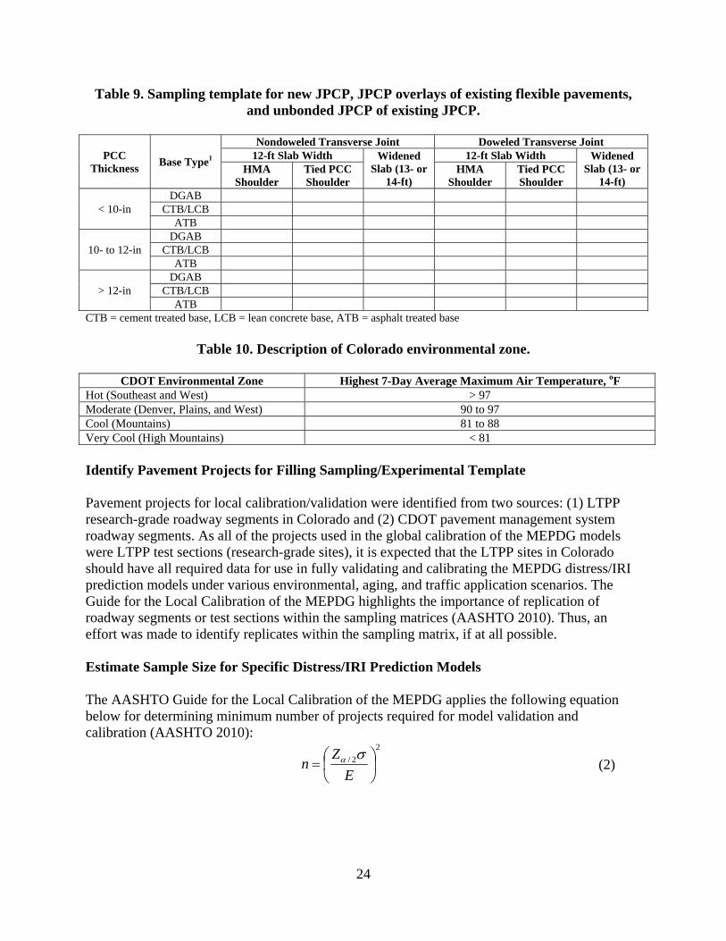
24

Table 9. Sampling template for new JPCP, JPCP overlays of existing flexible pavements, and unbonded JPCP of existing JPCP.

PCC Thickness

Base Type1

Nondoweled Transverse Joint Doweled Transverse Joint 12-ft Slab Width Widened

Slab (13- or 14-ft)

12-ft Slab Width Widened Slab (13- or

14-ft) HMA

Shoulder Tied PCC Shoulder

HMA Shoulder

Tied PCC Shoulder

< 10-in DGAB

CTB/LCB ATB

10- to 12-in DGAB

CTB/LCB ATB

> 12-in DGAB

CTB/LCB ATB

CTB = cement treated base, LCB = lean concrete base, ATB = asphalt treated base

Table 10. Description of Colorado environmental zone.

CDOT Environmental Zone Highest 7-Day Average Maximum Air Temperature, oF Hot (Southeast and West) > 97 Moderate (Denver, Plains, and West) 90 to 97 Cool (Mountains) 81 to 88 Very Cool (High Mountains) < 81 Identify Pavement Projects for Filling Sampling/Experimental Template Pavement projects for local calibration/validation were identified from two sources: (1) LTPP research-grade roadway segments in Colorado and (2) CDOT pavement management system roadway segments. As all of the projects used in the global calibration of the MEPDG models were LTPP test sections (research-grade sites), it is expected that the LTPP sites in Colorado should have all required data for use in fully validating and calibrating the MEPDG distress/IRI prediction models under various environmental, aging, and traffic application scenarios. The Guide for the Local Calibration of the MEPDG highlights the importance of replication of roadway segments or test sections within the sampling matrices (AASHTO 2010). Thus, an effort was made to identify replicates within the sampling matrix, if at all possible. Estimate Sample Size for Specific Distress/IRI Prediction Models The AASHTO Guide for the Local Calibration of the MEPDG applies the following equation below for determining minimum number of projects required for model validation and calibration (AASHTO 2010):

2

2/

E

Zn

(2)

25

where

2/Z = the score for having α percent of the data in the tails, i.e., P(|Z| > z) = α

for a 90 percent confidence interval 2/Z = 1.601

σ = performance indicator threshold (i.e., design threshold limit, see Table 11) E = tolerable bias at 90 percent reliability = 2/Z *SEE

SEE = distress/IRI models standard error of the estimate (see Table 11) For this project, design reliability and confidence interval were both assumed to be 90 percent. Table 11 presents a summary of distress/IRI thresholds and MEPDG nationally calibrated model SEE. Regardless of the minimum number of projects determined, the AASHTO Guide for the Local Calibration of the MEPDG recommends the minimum number of projects presented in Table 12 (AASHTO 2010).

Table 11. Summary of distress/IRI thresholds and MEPDG nationally calibrated model

SEE (obtained from AASHTO 2008).

Pavement Type

Performance Indicator

Performance Indicator Threshold (at 90%

Reliability) () SEE

Minimum No. of Projects Required for Validation & Local Calibration

New HMA and HMA-

overlaid HMA

Alligator cracking

20 percent lane area 5.01 percent 16

Transverse “thermal” cracking

Crack spacing > 100 ft. of 630 ft/mi

150 ft/mi 18

Rutting 0.4 in 0.107 in 14 IRI 169 in / mi 18.9 in/mi 80

New JPCP and JPCP subjected to CPR1

Faulting < 0.15 in 0.033 in 21 Transverse cracking

< 10 percent slabs 4.52 percent 5

IRI 169 in/mi 17.1 in/mi 98 1. CPR = concrete pavement repair or restoration.

26

Table 12. Minimum number of pavement projects required for the validation and local calibration (AASHTO 2010).

Pavement

Type Performance

Indicator Distress Classification

Minimum Number of Projects

Flexible

Alligator cracking Load-related cracking 30 Transverse “thermal”

cracking Non-load-related

cracking 30

Rutting Distortion 20 IRI Not applicable Not provided

Rigid

Faulting Distortion 20 Transverse cracking Load-related cracking 30

Punchouts Load-related cracking 30 IRI Not applicable Not provided

Composite HMA-

overlaid PCC

Reflection “transverse” cracking

Not classified 26

IRI Not applicable Not provided

27

CHAPTER 4. PROJECTS SELECTION AND DEVELOPMENT OF CLIMATE AND TRAFFIC DATABASE TO VALIDATE/CALIBRATE MEPDG MODELS The MEPDG implementation process involved developing a sampling template for project identification and calibration/validation database population. The two sources of data were the CDOT pavement management system and the LTPP database. This chapter describes work done to identify and select candidate projects for inclusion into the project calibration/validation database, as well as the development of the database. Identification and Selection of Pavement Projects Project Identification The LTPP database contained 72 research-type new HMA, HMA-overlaid existing HMA and JPCP, new JPCP, and unbonded JPCP overlay of JPCP projects in Colorado. A breakdown of the project types is presented in Figure 5. Note that some projects were double or triple counted, as they belonged to different pavement type categories at different time periods due to rehabilitation done over the course of their service life.

Figure 5. Breakdown of the LTPP project types in Colorado.

4

2 2

8

2 2

13

9

17

11

2

0

2

4

6

8

10

12

14

16

18

20

No. of Projects

The CDO9,954 misystem wlength ofpresented

Criteria f Pavemen

R

OT state highles are HMA

was divided if 0.1 miles (ad in Figure 6

for Pavemen

nt projects w

Research-grao Resea

globalo Thus,

analyso The so

databao The p

projec

hway systemA pavementsinto 112,009approximate6.

Figu

nt Projects Se

were selected

de pavemenarch-grade Ll models. they contain

sis. ole criterion ase is whethavement typcts in Colora

m consists of s, and 1,225 9 individual ply 500 ft). A

ure 6. CDOT

election

for the deve

t projects. TPP project

n at least at L

for inclusioer they repre

pe informatioado may be i

28

f 11,192 lanemiles are PCpavement m

A map showi

T state high

elopment of

s were used

Level 3 all in

on into the CDesent a pavemon presentedncluded in th

e miles of paCC pavemen

management sing the CDO

hway system

the project d

to develop a

nput data req

DOT local cment type of

d in Figure 5he project da

avement. Apnts. The entirsections with

OT state high

m.

database as f

and calibrate

quired for lo

calibration/vf interest. shows that atabase.

proximatelyre state highh an averagehway system

follows:

e the MEPD

ocal calibrati

validation

all 72 LTPP

y hway e

m is

G

ion

P

29

Pavement management system projects. o Must have available distress/IRI data from at least three condition surveys

collected within the past 7 to 10 years. This will ensure that all time-dependent inputs (i.e., material properties, traffic growth and accumulation, cyclic change in climate, cyclic change in groundwater and foundation properties) are properly taken into account in validation/calibration of the models.

o Consistency of distress/IRI measurements with MEPDG: Available distress/IRI data must be consistent in terms of both definition and precision with the MEPDG and, thus, LTPP protocols. This means that distress/IRI must be measured in accordance with the LTPP Distress Identification Manual (Miller & Bellinger 2003) or it should be possible to convert the reported distress/IRI into values equivalent to LTPP measurements.

o Consistency of materials, traffic, climate, and other measurements with MEPDG: All data used to establish the inputs for the models (including, material test results, climatic data, and traffic data) should be collected or measured in accordance with MEPDG standard procedures. Otherwise, it should be possible to convert as needed to be compatible with the MEPDG/LTPP.

o Roadway segments should be selected with the fewest number of structural layers and materials (e.g., one PCC layer, one or two HMA layers, one unbound base layer, and one subbase layer) to reduce the amount of testing and input required for material characterization.

o Roadway segments selected should as much as possible reflect CDOT construction and rehabilitation strategies. In other words, the roadway segments used to define SEE should include the range of construction practices (PCC curing, joint sawing, tack coat placement, bonding at layer interface, initial IRI, etc.) and rehabilitation practices (grinding equipment and specifications, joint repairs and dowel retrofit, joint sealant types applied for resealing, etc.).

o Roadway segments with and without HMA and PCC overlays are needed for the validation/calibration sampling template. Those segments that have detailed time-history distress data before and after rehabilitation should be given a higher priority for inclusion into the project database, as the proper characterization of the existing pavement prior to rehabilitation is key to developing accurate prediction models.

o Roadway segments or projects with HMA overlays should be limited to one HMA overlay during the monitoring period.

o Roadway segments that include non-conventional mixtures or layers should be included in the experimental sampling matrix to ensure that the model forms and calibration factors are representative of these mixtures. Non-conventional mixtures can include SMA, PMA, open-graded drainage layers, cement-aggregate mixtures, and high-strength PCC mixtures.

o Traffic data need to be well defined. Level 1 traffic inputs, normalized truck volume values, are required.

o HMA as-placed volumetric properties, gradation, and asphalt content need to be available from construction or project records. If not available, there should be information available to backcast initial air voids.

Descripti Based onwere selenoted thaHoweverthe requi Figures 7projects. projects. features o

Fig

ion of Select

n the selectioected from that not all of tr, such projered informat

7 through 9 sTables 13 thFigures 10 t

of the selecte

gure 7. Map

ted Projects

on criteria prhe LTPP andthe CDOT pacts were seletion can be a

show maps ohrough 15 prthrough 18 ped projects.

of selected

resented, a tod CDOT pavavement maected for incassembled th

of Colorado,resent basic present histo

pavement p

30

otal of 127 nvement manaanagement syclusion in thehrough field

along withdescriptive igrams show

projects alo

new and rehaagement sysystem projece project datand laborato

the locationinformation

wing the distr

ong the Colo

abilitated pavtem databas

cts had all thtabase on theory testing.

s of the selefor the selec

ribution of k

orado highw

vement projees. It must b

he required de assumption

cted pavemected paveme

key descriptiv

way system.

ects be data. n that

ent ent ve

Figur

F

re 8. Map sh

Figure 9. M

howing sele

Map showing

ected pavem

g rehabilitat

31

ment types al

ted pavemen

long the Co

nt projects

olorado high

in the Denv

hway system

ver area.

m.

32

Table 13. Inventory information (highway type, route, & direction) for selected projects.

Project Type

ARA ID

CDOT/LTPP ID

Project Name Highway

Type Route

No. Route ID Direction

CDOT 1 11328 IM 0704-178 Interstate 70 070A WB CDOT 2 11327 IM 0704-177 Interstate 70 070A WB CDOT 3 88452 IR(CX) 70-4(153) Interstate 70 070A EB CDOT 4 91044 FC-NH(CX) 024-3(036) U. S. 24 024G EB CDOT 5 12441 STA 0711-013 State 71 071D NB CDOT 6 91022 ACIM 070-5(53) Interstate 70 070A WB CDOT 7 13817 NH 0405-029 U. S. 40 040H EB CDOT 8 12685 NH 0505-033 U. S. 50 050B EB CDOT 9 13936 STA 1604-007 U. S. 160 160C EB CDOT 10 12393 BR 0251-150 Interstate 25 025A SB CDOT 11 12529 NH 0503-056 U. S. 50 050A EB CDOT 12 13390 IM 0252-342 Interstate 25 025A SB CDOT 13 10175 C 0243-042 U. S. 24 024G EB CDOT 14 13131 NH 0242-031 U. S. 24 024A EB CDOT 15 11959 STA 0242-026 U. S. 24 024A EB CDOT 16 13440 NH 0242-033 U. S. 24 024A EB CDOT 17 13932 IM 0252-358 Interstate 25 025A SB CDOT 18 12187 NHS 0831-076 State 83 083A NB CDOT 19 92021 NH(CX) 225-4(39) Interstate 225 225A NB CDOT 20 13353 STA 2254-063 Interstate 255 225A NB CDOT 21 91094 MU-STU 0030(006) State 30 030A EB CDOT 22 12297 NH 0061-066 U. S. 6 006G EB CDOT 23 11918 SP 0253-150 U. S. 36 036B WB CDOT 24 13356 STA 0704-199 Interstate 70 070A EB CDOT 25 10326 NH 2873-071 U. S. 287 287C NB CDOT 26 93216 NH(CX) 160-1(029) U. S. 160 160A EB CDOT 27 13959 STA 1191-017 State 119 119A WB CDOT 28 11865 NH 0341-046 U. S. 34 034A WB CDOT 29 89168 IR(CX) 076-1(150) Interstate 76 076A EB CDOT 30 11979 C 0761-170 Interstate 76 076A EB CDOT 31 13258 C 0403-043 U. S. 40 040B EB CDOT 32 12448 STA 006A-030 U. S. 6 006F WB CDOT 33 13435 STA 0061-069 State 9 009D SB CDOT 34 13513 NH 0242-034 U. S. 24 024A EB CDOT 35 13087 STR 135A-019 State 135 135A SB CDOT 36 13880 PLH 149A-020 State 149 149A SB CDOT 37 92976 NH(CX) 160-2(049) U. S. 160 160A EB CDOT 38 13505 STA 1602-084 U. S. 160 160A WB CDOT 39 11970 NH 1601-046 U. S. 160 160A WB CDOT 41 13325 NH 0501-045 U. S. 50 050A EB CDOT 42 12153 NH 0501-038 U. S. 50 050A EB CDOT 43 13085 PLH 139A-026 State 139 139A SB CDOT 44 11213 PLH 139A-023 State 139 139A NB CDOT 45 13106 STA 0641-011 State 64 064A WB CDOT 46 00000 I70-1(44) 89 Interstate 70 070A WB CDOT 47 12018 STR 131A-024 State 131 131B SB

33


Project Type

ARA ID

CDOT/LTPP ID


Type Route


CDOT 48 13866 STA 131A-028 State 131 131B NB CDOT 49 13864 STA 0821-063 State 82 082A WB CDOT 50 11780 HB 0821-047 State 82 082A EB CDOT 51 12271 SP 0821-053 State 82 082A WB CDOT 52 12321 STA 079A-009 State 79 079B NB CDOT

53 84076

FCUNH(CX)CY287-3(37)

U. S. 287 287C

NB

CDOT 54 11546 NH 2854-063 U. S. 285 285D NB CDOT 55 93015 NH(CX) 285-4(48) U. S. 285 285D NB LTPP 56 8_0213_1 LTPP Interstate 76 N/A EB LTPP 57 8_0214_1 LTPP Interstate 76 N/A EB LTPP 58 8_0215_1 LTPP Interstate 76 N/A EB LTPP 59 8_0216_1 LTPP Interstate 76 N/A EB LTPP 60 8_0217_1 LTPP Interstate 76 N/A EB LTPP 61 8_0218_1 LTPP Interstate 76 N/A EB LTPP 62 8_0219_1 LTPP Interstate 76 N/A EB LTPP 63 8_0220_1 LTPP Interstate 76 N/A EB LTPP 64 8_0221_1 LTPP Interstate 76 N/A EB LTPP 65 8_0222_1 LTPP Interstate 76 N/A EB LTPP 66 8_0223_1 LTPP Interstate 76 N/A EB LTPP 67 8_0224_1 LTPP Interstate 76 N/A EB LTPP 68 8_0259_1 LTPP Interstate 76 N/A EB LTPP 69 8_0501_1 LTPP Interstate 70 N/A EB LTPP 70 8_0501_2 LTPP Interstate 70 N/A EB LTPP 71 8_0502_1 LTPP Interstate 70 N/A EB LTPP 72 8_0502_2 LTPP Interstate 70 N/A EB LTPP 73 8_0503_1 LTPP Interstate 70 N/A EB LTPP 74 8_0503_2 LTPP Interstate 70 N/A EB LTPP 75 8_0504_1 LTPP Interstate 70 N/A EB LTPP 76 8_0504_2 LTPP Interstate 70 N/A EB LTPP 77 8_0505_1 LTPP Interstate 70 N/A EB LTPP 78 8_0505_2 LTPP Interstate 70 N/A EB LTPP 79 8_0506_1 LTPP Interstate 70 N/A EB LTPP 80 8_0506_2 LTPP Interstate 70 N/A EB LTPP 81 8_0507_1 LTPP Interstate 70 N/A EB LTPP 82 8_0507_2 LTPP Interstate 70 N/A EB LTPP 83 8_0508_1 LTPP Interstate 70 N/A EB LTPP 84 8_0508_2 LTPP Interstate 70 N/A EB LTPP 85 8_0509_1 LTPP Interstate 70 N/A EB LTPP 86 8_0509_2 LTPP Interstate 70 N/A EB LTPP 87 8_0559_1 LTPP Interstate 70 N/A EB LTPP 88 8_0559_2 LTPP Interstate 70 N/A EB LTPP 89 8_0560_1 LTPP Interstate 70 N/A EB LTPP 90 8_0560_2 LTPP Interstate 70 N/A EB LTPP 91 8_0811_1 LTPP Ramp N/A EB LTPP 92 8_0812_1 LTPP Ramp N/A EB

34


Project Type

ARA ID

CDOT/LTPP ID


Type Route


LTPP 93 8_1029_1 LTPP U. S. 40 N/A WB LTPP 94 8_1029_5 LTPP U. S. 40 N/A WB LTPP 95 8_1047_1 LTPP State 64 N/A WB LTPP 96 8_1047_2 LTPP State 64 N/A WB LTPP 97 8_1053_1 LTPP U. S. 50 N/A NB LTPP 98 8_1053_2 LTPP U. S. 50 N/A NB LTPP 99 8_1057_1 LTPP State 141B N/A SB LTPP 100 8_2008_1 LTPP U. S. 50 N/A WB LTPP 101 8_3032_1 LTPP Interstate 70 N/A EB LTPP 102 8_6002_1 LTPP Interstate 25 N/A NB LTPP 103 8_6002_2 LTPP Interstate 25 N/A NB LTPP 104 8_6013_1 LTPP U. S. 14 N/A EB LTPP 105 8_7035_1 LTPP Interstate 70 N/A EB LTPP 106 8_7035_2 LTPP Interstate 70 N/A EB LTPP 107 8_7036_1 LTPP Interstate 70 N/A EB LTPP 108 8_7776_1 LTPP Interstate 70 N/A EB LTPP 109 8_7780_1 LTPP U. S. 24 N/A WB LTPP 110 8_7780_2 LTPP U. S. 24 N/A WB LTPP 111 8_7781_1 LTPP U. S. 50 N/A WB LTPP 112 8_7781_2 LTPP U. S. 50 N/A WB LTPP 113 8_7783_1 LTPP Interstate 70 N/A EB LTPP 114 8_7783_3 LTPP Interstate 70 N/A EB LTPP 115 8_9019_1 LTPP Interstate 25 N/A NB LTPP 116 8_9020_1 LTPP Interstate 25 N/A SB LTPP 117 8_A310_1 LTPP U. S. 50 N/A NB LTPP 118 8_A310_2 LTPP U. S. 50 N/A NB LTPP 119 8_A320_1 LTPP U. S. 50 N/A NB LTPP 120 8_A330_1 LTPP U. S. 50 N/A NB LTPP 121 8_A340_1 LTPP U. S. 50 N/A NB LTPP 122 8_A350_1 LTPP U. S. 50 N/A NB LTPP 123 8_B310_1 LTPP U. S. 50 N/A WB LTPP 124 8_B310_2 LTPP U. S. 50 N/A WB LTPP 125 8_B320_1 LTPP U. S. 50 N/A WB LTPP 126 8_B330_1 LTPP U. S. 50 N/A WB LTPP 127 8_B350_1 LTPP U. S. 50 N/A WB

35

Table 14. Inventory information (CDOT region, county, highway functional class, & no. of lanes) for selected projects.

Project Type

ARA ID

CDOT/LTPP ID

Begin MP CDOT Region

County Highway Functional Class

CDOT 1 11328 309.00 1 Adams Rural principal arterial-Interstate CDOT 2 11327 312.00 1 Arapahoe Rural principal arterial-Interstate CDOT 3 88452 330.00 1 Arapahoe Rural principal arterial-Interstate CDOT 4 91044 375.80 1 Elbert Rural major collector CDOT 5 12441 107.00 1 Lincoln Rural minor collector CDOT 6 91022 440.00 1 Kit Carson Rural principal arterial-Interstate CDOT 7 13817 471.00 1 Cheyenne Rural major collector CDOT 8 12685 442.00 2 Prowers Rural major collector CDOT 9 13936 350.00 2 Las Animas Rural minor collector CDOT 10 12393 47.10 2 Huerfano Rural principal arterial-Interstate CDOT 11 12529 299.00 2 Pueblo Rural Major Collector CDOT 12 13390 139.50 2 El Paso Urban principal arterial-Interstate CDOT 13 10175 309.10 2 El Paso Urban principal arterial-other CDOT 14 13131 280.00 2 Teller Rural major collector CDOT 15 11959 283.30 2 Teller Rural major collector CDOT 16 13440 288.00 2 Teller Rural major collector CDOT 17 13932 155.00 2 El Paso Rural principal arterial-Interstate CDOT 18 12187 67.30 6 Arapahoe Urban principal arterial-other CDOT 19 92021 11.10 6 Adams Urban principal arterial-Interstate CDOT 20 13353 6.00 6 Arapahoe Urban principal arterial-Interstate CDOT 21 91094 11.40 6 Arapahoe Urban major collector CDOT 22 12297 284.30 6 Denver Urban major collector CDOT 23 11918 56.70 6 Adams Urban principal arterial-other CDOT 24 13356 281.00 6 Denver Urban principal arterial-Interstate CDOT 25 10326 301.40 4 Boulder Urban principal arterial-other CDOT 26 93216 38.95 5 Montezuma Urban principal arterial-other CDOT 27 13959 40.00 4 Boulder Rural principal arterial-other CDOT 28 11865 139.00 4 Weld Rural major collector CDOT 29 89168 61.00 4 Morgan Rural principal arterial-Interstate CDOT 30 11979 86.00 4 Morgan Rural principal arterial-Interstate CDOT 31 13258 272.20 1 Jefferson Rural major collector CDOT 32 12448 229.00 1 Clear Creek Rural minor collector CDOT 33 13435 103.20 1 Summit Urban major collector CDOT 34 13513 245.00 1 Park Rural major collector CDOT 35 13087 16.70 3 Gunnison Rural minor collector CDOT 36 13880 4.00 5 Rio Grande Rural minor collector CDOT 37 92976 182.80 5 Rio Grande Rural major collector CDOT 38 13505 96.00 5 La Plata Rural major collector CDOT 39 11970 72.00 5 La Plata Rural major collector CDOT 41 13325 73.00 3 Delta Urban major collector CDOT 42 12153 47.00 3 Mesa Rural major collector CDOT 43 13085 57.00 3 Rio Blanco Rural minor collector CDOT 44 11213 60.00 3 Rio Blanco Rural minor collector CDOT 45 13106 43.50 3 Rio Blanco Rural minor collector CDOT 46 00000 93.00 3 Garfield Rural principal arterial-Interstate

36


Project Type

ARA ID

CDOT/LTPP ID



CDOT 47 12018 66.00 3 Routt Rural Minor Collector CDOT 48 13866 33.00 3 Routt Rural Minor Collector CDOT 49 13864 4.50 3 Garfield Rural principal arterial-other CDOT 50 11780 26.10 3 Pitkin Rural principal arterial-other CDOT 51 12271 38.00 3 Pitkin Rural principal arterial-other CDOT 52 12321 7.50 1 Adams Rural major collector CDOT 53 84076 298.50 6 Broomfield Urban principal arterial-other CDOT 54 11546 242.00 1 Jefferson Rural principal arterial-other CDOT 55 93015 245.00 1 Jefferson Rural principal arterial-other

LTPP 56 8_0213_1 18.46 6 Adams Rural principal arterial-Interstate LTPP 57 8_0214_1 18.46 6 Adams Rural principal arterial-Interstate LTPP 58 8_0215_1 18.46 6 Adams Rural principal arterial-Interstate LTPP 59 8_0216_1 18.46 6 Adams Rural principal arterial-Interstate LTPP 60 8_0217_1 18.46 6 Adams Rural principal arterial-Interstate LTPP 61 8_0218_1 18.46 6 Adams Rural principal arterial-Interstate LTPP 62 8_0219_1 18.46 6 Adams Rural principal arterial-Interstate LTPP 63 8_0220_1 18.46 6 Adams Rural principal arterial-Interstate LTPP 64 8_0221_1 18.46 6 Adams Rural principal arterial-Interstate LTPP 65 8_0222_1 18.46 6 Adams Rural principal arterial-Interstate LTPP 66 8_0223_1 18.46 6 Adams Rural principal arterial-Interstate LTPP 67 8_0224_1 18.46 6 Adams Rural principal arterial-Interstate LTPP 68 8_0259_1 18.46 6 Adams Rural principal arterial-Interstate LTPP 69 8_0501_1 386.45 1 Lincoln Rural principal arterial-Interstate LTPP 70 8_0501_2 386.45 1 Lincoln Rural principal arterial-Interstate LTPP 71 8_0502_1 386.45 1 Lincoln Rural principal arterial-Interstate LTPP 72 8_0502_2 386.45 1 Lincoln Rural principal arterial-Interstate LTPP 73 8_0503_1 386.45 1 Lincoln Rural principal arterial-Interstate LTPP 74 8_0503_2 386.45 1 Lincoln Rural principal arterial-Interstate LTPP 75 8_0504_1 386.45 1 Lincoln Rural principal arterial-Interstate LTPP 76 8_0504_2 386.45 1 Lincoln Rural principal arterial-Interstate LTPP 77 8_0505_1 386.45 1 Lincoln Rural principal arterial-Interstate LTPP 78 8_0505_2 386.45 1 Lincoln Rural principal arterial-Interstate LTPP 79 8_0506_1 386.45 1 Lincoln Rural principal arterial-Interstate LTPP 80 8_0506_2 386.45 1 Lincoln Rural principal arterial-Interstate LTPP 81 8_0507_1 386.45 1 Lincoln Rural principal arterial-Interstate LTPP 82 8_0507_2 386.45 1 Lincoln Rural principal arterial-Interstate LTPP 83 8_0508_1 386.45 1 Lincoln Rural principal arterial-Interstate LTPP 84 8_0508_2 386.45 1 Lincoln Rural principal arterial-Interstate LTPP 85 8_0509_1 386.45 1 Lincoln Rural principal arterial-Interstate LTPP 86 8_0509_2 386.45 1 Lincoln Rural principal arterial-Interstate LTPP 87 8_0559_1 386.45 1 Lincoln Rural principal arterial-Interstate LTPP 88 8_0559_2 386.45 1 Lincoln Rural principal arterial-Interstate LTPP 89 8_0560_1 386.45 1 Lincoln Rural principal arterial-Interstate LTPP 90 8_0560_2 386.45 1 Lincoln Rural principal arterial-Interstate LTPP 91 8_0811_1 6 Adams Rural local collector

37


Project Type

ARA ID

CDOT/LTPP ID



LTPP 92 8_0812_1 6 Adams Rural local collector LTPP 93 8_1029_1 69.75 3 Moffat Rural principal arterial-other LTPP 94 8_1029_5 69.75 3 Moffat Rural principal arterial-other LTPP 95 8_1047_1 16.6 3 Rio Blanco Rural major collector LTPP 96 8_1047_2 16.6 3 Rio Blanco Rural major collector LTPP 97 8_1053_1 75.3 3 Delta Rural principal arterial-other LTPP 98 8_1053_2 75.3 3 Delta Rural principal arterial-other LTPP 99 8_1057_1 160.65 3 Mesa Urban principal arterial - other LTPP 100 8_2008_1 401.93 2 Bent Rural principal arterial-other LTPP 101 8_3032_1 95.75 3 Garfield Rural principal arterial-Interstate LTPP 102 8_6002_1 106.35 2 Pueblo Rural principal arterial-Interstate LTPP 103 8_6002_2 106.35 2 Pueblo Rural principal arterial-Interstate LTPP 104 8_6013_1 235.4 4 Logan Urban principal arterial-other LTPP 105 8_7035_1 286.25 1 Adams Rural principal arterial-Interstate LTPP 106 8_7035_2 286.25 1 Adams Rural principal arterial-Interstate LTPP 107 8_7036_1 308.55 1 Arapahoe Rural principal arterial-Interstate LTPP 108 8_7776_1 290.3 1 Adams Rural principal arterial-Interstate LTPP 109 8_7780_1 291.26 2 El Paso Rural principal arterial-other LTPP 110 8_7780_2 291.26 2 El Paso Rural principal arterial-other LTPP 111 8_7781_1 402.18 2 Bent Rural principal arterial-other LTPP 112 8_7781_2 402.18 2 Bent Rural principal arterial-other LTPP 113 8_7783_1 67.66 3 Garfield Rural principal arterial-Interstate LTPP 114 8_7783_3 67.66 3 Garfield Rural principal arterial-Interstate LTPP 115 8_9019_1 246.5 4 Weld Rural principal arterial-Interstate LTPP 116 8_9020_1 256.4 4 Larimer Rural principal arterial-Interstate LTPP 117 8_A310_1 75.3 3 Delta Rural principal arterial-other LTPP 118 8_A310_2 75.3 3 Delta Rural principal arterial-other LTPP 119 8_A320_1 75.3 3 Delta Rural principal arterial-other LTPP 120 8_A330_1 75.3 3 Delta Rural principal arterial-other LTPP 121 8_A340_1 75.3 3 Delta Rural principal arterial-other LTPP 122 8_A350_1 75.3 3 Delta Rural principal arterial-other LTPP 123 8_B310_1 401.93 2 Bent Rural principal arterial-other LTPP 124 8_B310_2 401.93 2 Bent Rural principal arterial-other LTPP 125 8_B320_1 401.93 2 Bent Rural principal arterial-other LTPP 126 8_B330_1 401.93 2 Bent Rural principal arterial-other LTPP 127 8_B350_1 401.93 2 Bent Rural principal arterial-other

38

Table 15. Inventory information (construction/rehab date, long/lat & elevation) for selected projects.

Project Type

ARA ID

CDOT/LTPP ID

Pavement Type Const. Year

Rehab Year

Latitude, deg

Longitude, deg.

Elev., ft

CDOT 1

11328 Unbonded JPCP overlay

over existing JPCP 1963 1998 39.7 -104.4 5406

CDOT 2



CDOT 3



CDOT 4 91044 New HMA 1998 39.3 -103.7 5421 CDOT

5 12441

HMA overlay (cold in place recycle) over existing HMA

1977 2000 39.3 -103.7 5517

CDOT 6

91022 JPCP overlay over existing

HMA 1969 1995 39.3 -102.2 4091

CDOT 7

13817 HMA overlay (cold in place recycle) over existing HMA

1966 2002 38.8 -102.3 4223

CDOT 8

12685 Superpave HMA overlay

over existing HMA 1973 2001 38.1 -102.5 3577

CDOT 9



CDOT 10 12393 New HMA 2001 37.6 -104.7 6245 CDOT

11 12529

HMA overlay (hot in place recycle) over existing HMA

1973 1999 38.4 -104.9 5191

CDOT 12 13390 New HMA 2001 38.8 -104.8 5930 CDOT 13 10175 New JPCP 1996 38.8 -104.7 6084 CDOT 14 13131 New HMA 2002 39.0 -105.1 9082 CDOT 15 11959 New HMA 2002 39.0 -105.1 8710 CDOT

16 13440

Superpave HMA overlay over existing HMA

1975 2001 39.0 -105.0 8060

CDOT 17

13932 HMA overlay (hot in place recycle) over existing HMA

1953 2002 39.0 -104.8 6618

CDOT 18

12187 HMA overlay of existing

JPCP 1984 1999 39.6 -104.8 5689

CDOT 19 92021 New JPCP 1994 39.8 -104.8 5355 CDOT

20 13353

AC overlay over existing JPCP

1971 2002 39.7 -104.8 5600

CDOT 21 91094 New HMA 1999 39.7 -104.8 5475 CDOT

22 12297

SMA overlay over existing HMA

1980 2000 39.7 -105.0 5273

CDOT 23 11918 New HMA 2001 39.8 -105.0 5272 CDOT

24 13356

HMA overlay of existing JPCP

1963 2002 39.8 -104.9 5325

CDOT 25 10326 New JPCP 1996 40.0 -105.1 5218 CDOT 26 93216 New JPCP 1994 37.3 -108.6 6180 CDOT

27 13959


1969 2002 40.0 -105.3 5627

CDOT 28 11865 New HMA 2001 40.3 -104.2 4486 CDOT 29 89168 Unbonded JPCP overlay of 1959 1992 40.2 -104.1 4570

39


Project Type

ARA ID

CDOT/LTPP ID


Rehab Year

Latitude, deg

Longitude, deg.

Elev., ft

existing JPCP

CDOT 30

11979 HMA overlay of existing

JPCP 1962 1998 40.3 -103.7 4262

CDOT 31



CDOT 32


1986 1999 39.7 -105.9 10869

CDOT 33



CDOT 34


1969 2003 39.0 -105.7 8911

CDOT 35 13087 New HMA 2001 38.8 -106.9 8448 CDOT

36 13880


1953 2002 37.7 -106.7 8264

CDOT 37 92976 New HMA 1999 37.6 -106.7 8468 CDOT

38 13505


1975 2001 37.2 -107.7 6874

CDOT 39

11970 HMA overlay (cold in place recycle) over existing HMA

1971 2001 37.3 -108.1 8232

CDOT 41


1936 2001 38.7 -108.0 5091

CDOT 42 12153 New HMA 2002 38.9 -108.4 4967 CDOT 43 13085 New HMA 2002 39.9 -108.7 5858 CDOT 44 11213 New HMA 2000 39.9 -108.7 5750 CDOT

45 13106


1962 2001 40.2 -108.4 5545

CDOT 46 00000 New JPCP 1976 39.5 -107.7 5350 CDOT 47 12018 New HMA 2002 40.4 -106.8 6866 CDOT

48 13866


1962 2002 40.1 -106.8 8338

CDOT 49


1955 2002 39.5 -107.3 5988

CDOT 50 11780 New HMA 2000 39.3 -107.0 6852 CDOT 51 12271 New HMA 2002 39.2 -106.9 7825 CDOT

52 12321


1983 1999 39.8 -104.4 5310

CDOT 53 84076 New JPCP 1995 39.9 -105.1 5460 CDOT 54 11546 New JPCP 1999 39.6 -105.2 7436 CDOT 55 93015 New JPCP 1997 39.6 -105.2 6966

LTPP 56 8_0213_1 New JPCP 1993 39.9 -104.8 5077

LTPP 57 8_0214_1 New JPCP 1993 39.9 -104.8 5077

LTPP 58 8_0215_1 New JPCP 1993 39.9 -104.8 5077

LTPP 59 8_0216_1 New JPCP 1993 39.9 -104.8 5077

40


Project Type

ARA ID

CDOT/LTPP ID


Rehab Year

Latitude, deg

Longitude, deg.

Elev., ft

LTPP 60 8_0217_1 New JPCP 1993 39.9 -104.8 5077

LTPP 61 8_0218_1 New JPCP 1993 39.9 -104.8 5077

LTPP 62 8_0219_1 New JPCP 1993 39.9 -104.8 5077

LTPP 63 8_0220_1 New JPCP 1993 39.9 -104.8 5077

LTPP 64 8_0221_1 New JPCP 1993 39.9 -104.8 5077

LTPP 65 8_0222_1 New JPCP 1993 39.9 -104.8 5077

LTPP 66 8_0223_1 New JPCP 1993 40.0 -104.8 5077

LTPP 67 8_0224_1 New JPCP 1993 39.9 -104.8 5077

LTPP 68 8_0259_1 New JPCP 1993 40.0 -104.8 5077

LTPP 69 8_0501_1 New HMA 1974 39.3 -103.2 5128

LTPP 70 8_0501_2

HMA overlay of existing HMA 1974 1991

39.3 -103.2 5128

LTPP 71 8_0502_1 New HMA 1974 39.3 -103.2 5128

LTPP 72 8_0502_2


39.3 -103.2 5128

LTPP 73 8_0503_1 New HMA 1974 39.3 -103.2 5128

LTPP 74 8_0503_2


39.3 -103.2 5128

LTPP 75 8_0504_1 New HMA 1974 39.3 -103.2 5128

LTPP 76 8_0504_2


39.3 -103.2 5128

LTPP 77 8_0505_1 New HMA 1974 39.3 -103.2 5128

LTPP 78 8_0505_2


39.3 -103.2 5128

LTPP 79 8_0506_1 New HMA 1974 39.3 -103.2 5128

LTPP 80 8_0506_2


39.3 -103.2 5128

LTPP 81 8_0507_1 New HMA 1974 39.3 -103.2 5128

LTPP 82 8_0507_2


39.3 -103.2 5128

LTPP 83 8_0508_1 New HMA 1974 39.3 -103.2 5128

LTPP 84 8_0508_2


39.3 -103.2 5128

LTPP 85 8_0509_1 New HMA 1974 39.3 -103.2 5128

LTPP 86 8_0509_2


39.3 -103.2 5128

LTPP 87 8_0559_1 New HMA 1974 39.3 -103.2 5128

LTPP 88 8_0559_2


39.3 -103.2 5128

LTPP 89 8_0560_1 New HMA 1974 39.3 -103.2 5128

LTPP 90 8_0560_2


39.3 -103.2 5128

41


Project Type

ARA ID

CDOT/LTPP ID


Rehab Year

Latitude, deg

Longitude, deg.

Elev., ft

LTPP 91 8_0811_1 New JPCP 1993 39.9 -104.8 5095

LTPP 92 8_0812_1 New JPCP 1993 39.9 -104.8 5095

LTPP 93 8_1029_1 New HMA 1972 40.5 -107.9 5920

LTPP 94 8_1029_5


40.5 -107.9 5920

LTPP 95 8_1047_1 New HMA 1983 40.1 -108.8 5260

LTPP 96 8_1047_2


40.1 -108.8 5260

LTPP 97 8_1053_1 New HMA 1984 38.7 -108.0 5140

LTPP 98 8_1053_2


38.7 -108.0 5140

LTPP 99 8_1057_1 New HMA 1985 39.1 -108.5 4586

LTPP 100 8_2008_1 New HMA 1972 38.1 -103.2 3894

LTPP 101 8_3032_1 New JPCP 1977 39.5 -107.7 5345

LTPP 102 8_6002_1 New HMA 1958 38.4 -104.6 4904

LTPP 103 8_6002_2


38.4 -104.6 4904

LTPP 104 8_6013_1 New HMA 1965 40.6 -103.2 3935

LTPP 105 8_7035_1

HMA overlay of JPCP (New) 1965

39.8 -104.8 5500

LTPP 106 8_7035_2

HMA overlay of existing JPCP 1965 1994

39.8 -104.8 5500

LTPP 107 8_7036_1

HMA overlay of JPCP (New) 1961

39.7 -104.3 5380

LTPP 108 8_7776_1 New JPCP 1988 39.7 -104.7 5280

LTPP 109 8_7780_1 New HMA 1973 38.9 -105.0 7400

LTPP 110 8_7780_2


38.9 -105.0 7400

LTPP 111 8_7781_1 New HMA 1972 38.1 -103.2 3894

LTPP 112 8_7781_2


38.1 -103.2 3894

LTPP 113 8_7783_1 New HMA 1984 39.4 -108.1 5000

LTPP 114 8_7783_3


39.4 -108.1 5000

LTPP 115 8_9019_1

Unbonded JPCP overlay of existing JPCP 1966

40.2 -105.0 4970

LTPP 116 8_9020_1

Unbonded JPCP overlay of existing JPCP 1962

40.4 -105.0 4550

LTPP 117 8_A310_1 New HMA 1984 38.7 -108.0

LTPP 118 8_A310_2


38.7 -108.0

LTPP 119 8_A320_1 New HMA 1984 38.7 -108.0

LTPP 120 8_A330_1 New HMA 1984 38.7 -108.0

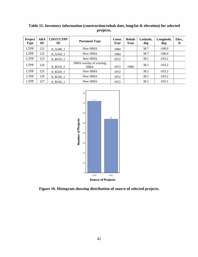
Table

Project Type

LTPP

LTPP

LTPP

LTPP

LTPP

LTPP

LTPP

e 15. Invent

ARA ID

CDO

121 8_A122 8_A123 8_B

124 8_B

125 8_B126 8_B127 8_B

Figure 10.

tory informa

OT/LTPP ID

A340_1

A350_1

B310_1

B310_2 H

B320_1

B330_1

B350_1

. Histogram

ation (const

Pavement

New HM

New HM

New HMHMA overlay

HMANew HM

New HM

New HM

m showing di

42

truction/rehprojects.

t Type

MA

MA

MA of existing

A MA

MA

MA

istribution o

hab date, lon.

Const. Year

ReYe

1984

1984

1972

1972 19

1972

1972

1972

of source of

ng/lat & ele

ehab ear

Latitudeg

38.7

38.7

38.1

990 38.1

38.1

38.1

38.1

f selected pr

evation) for

de, g

Longitudeg.

7 -108.

7 -108.

1 -103.

1 -103.

1 -103.

1 -103.

1 -103.

rojects.

selected

ude, .

Elev., ft

0

0

2

2

2

2

2

Figure 1

Figu

12. Histogra

ure 11. Hist

am showing

togram show

distributio

43

wing distrib

n of CDOTlocated.

bution of rou

regions in w

ute signage.

which selec

.

cted projectss are

Figu

Figure 14

ure 13. Histo

4. Histogram

ogram show

m showing d

44

wing distribu

distribution

ution of pav

of highway

vement type

y functional

e.

l class.

Figure 15

Figure 16. H

5. Histogram

Histogram

m showing d

showing dis

45

distribution

stribution o

n of facility n

of pavement

number of l

t location ele

lanes.

evation.

Figure 1

Pavemendefine ininformatitypes of itemplatesall possibfactorial adequaterepresentconstruct

Figure 17.

18. Histogra

nt design and detail the prion was usedinterest for us are presentble high, aveexperimenta to meet the ted Coloradotion practice

. Histogram

am showing

d inventory droject type, sd to populateuse in MEPDted in Tableserage, low coal design). Hgoals for m

o pavement des.

m showing di

g distributio

data were obstructure, laye the samplinDG model vas 16 and 17.ombinations

However, theodel validatidesign pract

46

istribution o

on of pavem

year.

btained from yer types andng templatesalidation/calThere were of all the sa

e partial expeion/calibratioices, materia

of original c

ment rehabili

LTPP data td materials, s developed libration. Thnot enough

ampling temperimental deon, and the pals propertie

construction

itation (ove

tables and Clocation, etcto identify ae populated projects sele

plates input sign obtaineprojects sele

es, site condi

n year.

rlay placem

CDOT recordc. The assemand select prsampling ected to achfactors (i.e.,

ed was deemected collectiitions, and

ment)

ds to mbled roject

ieve , full

med ively

47

Table 16. Experimental template populated with new HMA and HMA-overlaid HMA pavement projects for use in MEPDG flexible pavement model calibration/validation in

Colorado.

HMA Thickness

Binder Type

Climate Zone3

Subgrade Type Fine-Grained Soil Coarse-Grained Soil

Conv. HMA1 Full-

Depth HMA2

Conv. HMA1 Full-

Depth HMA2

< 4-in

Neat Hot/Moderate

1047_1, 1057_1, 2008_1, 7781_1, B310_1, B320_1 B350_1, 0501_2, 0505_2, 0506_2, A310_2, 1047_2 6002_1, 7781_2, 7783_3,

9-13936, 22-12297

0502_2, 0509_2 7780_1, 7-13817

Cool 38-13505 31-13258, 34-13513 Very Cool 33-13435


41-13325, 45-13106 48-13866

49-13864

Cool 44-11213 Very Cool 36-13880 32-12448

4- to 8-in

Neat Hot/Moderate

0501_1, 0504_1, 0505_1, 0506_1, 0507_1, 0559_1 1053_1, 7783_1, A310_1, A320_1, A330_1, A340-1 A350_1, B330_1, 0504_2, 0507_2, 0559_2, B310_2

1053_2, 5-12441, 8-12685, 11-12529

0502_1, 0503_1 0508_1, 0509_1 0560_1, 1029_1 1029_5, 0503_2 0508_2, 0560_2

Cool 50-11780 Very Cool 15-11959, 39-11970 16-13440 14-13131


47-12018 6002_2, 52-12321

4-91044 43-13085, 27-13959

Cool 51-12271, 17-13932 Very Cool 37-92976, 35-13087

> 8-in

Neat Hot/Moderate 12-13390 21-91094

Cool Very Cool

Modified Hot/Moderate 10-12393 42-12153, 28-11865 23-11918

Cool Very Cool

1. Conventional HMA is typically and HMA layer placed over thick dense graded aggregate base (DGAB) over the prepared subgrade. Conventional HMA could also include surface treatments (chip seal, fog seal, slurry seal or crack seal) on conventional HMA. 2. Full-depth HMA is typically HMA over asphalt treated base (dense or drainable) over a prepared subgrade. 3. See Table 10.

48

Table 17. Experimental template populated with new JPCP, JPCP overlays of flexible pavements, and unbonded JPCP of JPCP projects for use in MEPDG JPCP model

calibration/validation in Colorado.

PCC Thickness

Base Type1

Nondoweled Transverse Joint Dowelled Transverse Joint 12-ft Slab Width Widened

Slab (13- or 14-ft)

12-ft Slab Width Widened Slab (13- or

14-ft) HMA

Shoulder Tied PCC Shoulder

HMA Shoulder

Tied PCC Shoulder

< 10-in

DGAB 13-10175

CTB/LCB 26-93216 0213, 0214

0811 55-93015 54-11546 25-10326

ATB 90192 90202

3032 29-891682

0217, 0218 0219

53-84076

10 to 12-in

DGAB 18-121873 0221, 0222 CTB/LCB 0259

ATB 7776, 0215

0216, 0812 19-92021

> 12-in DGAB 0220 3-884522

CTB/LCB 0223, 0224 6-910223 ATB

1. CTB = cement treated base, LCB = lean concrete base, ATB = asphalt treated base 2. Unbonded JPCP 3. JPCP over existing HMA Extracting, Assembling, and Evaluating Project Data (Project Database Development) The MEPDG requires input data in several categories. For this implementation project, pavement data were obtained primarily from the following sources:

LTPP inventory, traffic, climate, materials, maintenance/rehabilitation databases. LTPP construction guidelines and reports. CDOT Online Transportation Information System (OTIS) (data from over 120 permanent

automated traffic recorder [ATR] and 13 continuous weigh-in-motion [WIM] sites). CDOT pavement management system data tables. CDOT design/construction reports. CDOT construction quality assurance (QA) testing databases. CDOT pavement research and forensic examination reports. Field testing/surveys and laboratory testing of extracted materials. Colorado Climate Center. NCDC database and the USDA NRCS SSURGO database.

Details of data sources are presented in Tables 18 and 19.

49

Table 18. LTPP sources of MEPDG input data for development of CDOT MEPDG calibration/validation database.

Data Category Source of Information (LTPP Data Tables)

Inventory

INV_GENERAL, INV_AGE, INV_ID, SPS_GENERAL, SPS _ID, SPS2_PCC_PLACEMENT_DATA SPS8_PCC_PLACEMENT_DATA SPS5_OVERLAY, SECTION_COORDINATES

Structure definition TST_L05B

Traffic

TRF_HIST_EST_ESAL, TRF_MON_EST_ESAL TRF_MEPDG_AADTT_LTPP_LN, TRF_MEPDG_AX_DIST_ANL TRF_MEPDG_AX_PER_TRUCK, TRF_MEPDG_HOURLY_DIST TRF_MEPDG_MONTH_ADJ_FACTR, TRF_MEPDG_VEH_CLASS_DIST TRF_MONITOR_AXLE_DISTRIB, TRF_MONITOR_LTPP_LN

Mat

eria

ls

Layer type and materials description

TST_L05B

In situ FWD deflection testing

MON_DEFL_DEV_CONFIG, MON_DEFL_LOC_INFO MON_DEFL_TEMP_VALUES, FWD_Drop_Data_States_AL_ID

Asphalt INV_PMA_ASPHALT, TST_AG04, RHB_ACO_PROP, RHB_HMRAP_NEW_AC_PROP

PCC INV_PCC_MIXTURE, TST_PC01, TST_PC02, TST_PC03, TST_PC04, TST_PC09, SPS Experiment Guidelines

Chemically stabilized TST_TB02 Unbound aggregate & subgrade soils

TST_SS01_UG01_UG02, TST_UG04_SS03

Climate NCDC & Colorado Climate Center

Design INV_PCC_JOINT, SPS Experiment Guidelines, SPS-1, -2, -5, -6 construction reports, INV_GENERAL, SPS_GENERAL

Construction SPS-1, -2, -3, -5, -6, -9 Construction reports

Per

form

ance

HMA alligator cracking MON_DIS_AC_REV HMA transverse “thermal” cracking

MON_DIS_AC_REV

Total rutting MON_T_PROF_INDEX_SECTION JPCP transverse “slab” cracking

MON_DIS_JPCC_REV

JPCP transverse joint faulting

MON_DIS_JPCC_FAULT_SECT

IRI MON_PROFILE_MASTER

50

Table 19. CDOT sources of MEPDG input data for development of CDOT MEPDG calibration/validation database.

Data Category Source of Information (CDOT Data Tables)

Inventory CDOT data libraries

Structure definition CDOT data libraries, construction QA records/database, Resident Materials Engineer files

Traffic CDOT OTIS, WIM/ATR data

Mat

eria

ls

Layer type and materials description

CDOT data libraries, construction QA records/database, Resident Materials Engineer files

Asphalt Laboratory testing PCC Laboratory testing Chemically stabilized

Insitu FWD deflection testing and characterization of materials properties, MEPDG defaults

Unbound aggregate & subgrade soils

Insitu FWD deflection testing and characterization of materials properties

Climate NCDC & CDOT weather stations climate data files

Design CDOT data libraries, construction QA records/database, Resident Materials Engineer files

Construction CDOT data libraries, construction QA records/database, Resident Materials Engineer files

Per

form

ance

HMA alligator cracking Manual visual distress surveys, coring and examination of cores, CDOT pavement management system

HMA transverse “thermal” cracking

Manual visual distress surveys, coring and examination of cores, CDOT pavement management system

Total rutting Manual visual distress surveys & trenching, CDOT pavement management system JPCP transverse “slab” cracking

Manual visual distress surveys, coring and examination of cores, CDOT pavement management system

JPCP transverse joint faulting

Manual visual distress surveys, CDOT pavement management system

IRI Profile measurements and computation of smoothness (IRI), CDOT pavement management system

Extraction and Assembly of Pertinent Data The first step in developing the project database for model validation/calibration was to extract relevant information from the various data sources identified in Tables 18 and 19. As the identified data/information came in various formats and standards (electronic and hard copies), a wide variety of software tools and methods was applied to extract pertinent data in an orderly and efficient manner. Data extraction basically consisted of the following steps:

1. For each selected project, define location references that many be used to extract data from the many sources identified in Tables 18 and 19. Examples of project location references used data extraction and assembly are as follows:

a. LTPP: SHRPID, STATE_CODE, CONSTRUCTION_NO (see Table 20). b. CDOT OTIS: ROUTE_NO, BEGIN MILEPOST, END MILEPOST (see Figure

19). c. NCDC & Colorado Climate Center: LATITUDE, LONGITUDE.

51

d. CDOT pavement management system: CDOT PMS ID, CDOT REGION, ROUTE_SIGN, ROUTE_NO, DIRECTION, BEGIN MILEPOST, END MILEPOST.

Note that multiple location references are required to extract data from different sources. 2. Develop basic database with as many location references as needed for each selected

project (see example in Table 20). 3. For each data source (in electronic or hard copy format) identify pertinent data (e.g.,

LTPP table TST_L05B contains information on pavement structure, layer thicknesses, and material description) and applicable location reference system.

4. Develop appropriate algorithms and routines as needed using database software tools (e.g., MS Access, MS Excel, SAS) for extracting pertinent data. Note that data in paper format (hard copy) was manually converted into electronic form before extraction and assembly in the project database. An example of the routines developed in MS Access and used for data extraction and assembly is presented in Figure 20.

Table 20. Example of multiple project location references used for data extraction and assembly.

CDOT

ID SHRP

ID CONST.

No. ROUTE

SIGN ROUTE

No. HWY DIRECTION

BEGIN MP

END MP

CDOT REGION

11328 N/A N/A Interstate 70 70A WB 309 308.8 1 11327 N/A N/A Interstate 70 70A WB 312 311.8 1 88452 N/A N/A Interstate 70 70A EB 330 330.2 1 91022 N/A N/A Interstate 70 70A WB 440 439.8 1 12393 N/A N/A Interstate 25 25A SB 47.1 46.9 2 13390 N/A N/A Interstate 25 25A SB 139.5 139.3 2 13932 N/A N/A Interstate 25 25A SB 155 154.8 2 92021 N/A N/A Interstate 255 255A NB 11.1 11.3 6 N/A 3032 1 Interstate 70 70 EB 95.75 3 N/A 6002 1 Interstate 25 25 NB 106.35 2 N/A 6002 2 Interstate 25 25 NB 106.35 2 N/A 1029 1 U.S. 40 40 WB 69.75 3 N/A 1029 5 U.S. 40 40 WB 69.75 3 N/A 1053 1 U.S. 50 50 NB 75.3 3 N/A 1053 2 U.S. 50 50 NB 75.3 3 N/A 2008 1 U.S. 50 50 WB 401.93 2 N/A

1057 1 State Route

141B 141B SB 160.65

3

N/A 6013 1 U.S. 14 14 EB 235.4 4

Figu

Figure

ure 19. CDO

e 20. Examp

OT OTIS gr

ple of the rou

raphic showex

utines develand

52

wing locationxtraction.

loped in MSd assembly.

n referencin

S Access and

ng used for

d used for d

traffic data

data extract

a

tion

53

Evaluation of Assembled Project Data and Final Project Database Development The assembled project database was reviewed and evaluated to determine the following:

Data deemed to be reasonable and accurate. Data deemed to be potentially anomalous, erroneous, or outliers. Missing data.

This was done using a variety of techniques, including:

Computing basic statistics (mean, max., min, standard deviation) for use in identifying outliers and erroneous data elements. In general, inputs that fell outside the range of mean + 3σ were deemed outliers.

Comparison of input data with engineering expectations (i.e., layer thickness must be greater than zero).

Developing time based plots of key variables to determine reasonableness of magnitudes and change in magnitude over time (see Figures 21 through 24).

Figure 21. Plot showing change in alligator (bottom-up fatigue) cracking over time for

CDOT project 12393.

Figure 22. Plot showing change in total rutting over time for CDOT project 12393.

BU C

rack

ing, %

Ln A

rea

0102030405060708090

100

Age, months

0 24 48 72 96 120 144 168 192 216 240

PTYPE=NewAC SHRPID=10-12393

PLOTTOTAL BUONLYREFLECT LTPP AC

Rut Depth, in

0.0

0.1

0.2

0.3

0.4

0.5

0.6

0.7

0.8

Age, mo

0 24 48 72 96 120 144 168 192 216 240

SHRPID=10-12393_calib

54

Figure 23. Plot showing change in average annual daily truck traffic (AADTT) over time for CDOT project 13258.

Figure 24. Plot showing change in backcalculated subgrade elastic modulus over time for

LTPP project 0501.

Data inputs deemed as outliers or erroneous were flagged and remedial action was taken, in the form of (1) replacing with more reasonable information from other sources or (2) removal from the project database without replacement, leaving only accurate and reasonable data in the project database. Thus, for each project, data elements not available in the project database were deemed missing and not available. Although agencies invest significant resources to compile and maintain vast amounts of data for use in pavement management, research, etc., for most situations it is virtually impossible to maintain a database that is complete with all records populated with reasonable, accurate data. Also, because of the complexity of the MEPDG, most agencies do not regularly maintain all the types of information required as inputs.

AADTT

40

60

80

100

120

140

160

180

Age, years

0 1 2 3 4 5 6 7 8 9

16,000

18,000

20,000

22,000

24,000

26,000

28,000

6/15/1994 10/28/1995 3/11/1997 7/24/1998 12/6/1999 4/19/2001 9/1/2002 1/14/2004

Backcalculated Subgrad

e Elastic M

odulus, psi

Test Date

55

Estimating Missing Data Evaluation of the assembled project database revealed considerable gaps in data required for MEPDG model validation/calibration. A summary of data availability is presented in Table 21. There are several methods of resolving gaps/missing data in a database. Below is a summary of some of the commonly applied strategies to resolve such situations:

Discarding Projects with Missing Data: Discarding projects with incomplete records/missing data is practical only when (1) the number of projects is very small compared to the total number of projects (say, less than 5 percent of projects), (2) the missing data for a given project are very expensive (e.g., 80 percent of all required data), or (3) the missing data are fundamental for successfully conducting analysis (e.g., definition of pavement structure is missing or traffic volume data). For this project, discarding projects with missing data was not a feasible option since none of the projects selected met any of the criteria described.

Estimation of Missing Data Element: Estimating missing data elements using correlations with other data elements (e.g., relating PCC flexural strength with compressive strength) is a very common practice for replacing missing data. The MEPDG provides several relationships for making such estimates and provides “national” defaults where the use of such relationships is not feasible.

Forensic Examination: Missing data elements for a given project can be obtained through forensic examination of the project (e.g., coring, extraction, of cores, and examination and testing to determine pavement structure, layer thicknesses, material types, etc.). Estimates of the missing data can also be obtained through constitution of similar materials in the laboratory and testing for the required properties/inputs.

The estimation of missing data and forensic examinations options were utilized as needed to acquire missing data. Work done to acquire missing data is presented in the following sections. Estimating Missing Traffic Data A full list of missing traffic data elements is provided in Table 21. Default Colorado estimates of the missing data were developed using traffic data from LTPP and CDOT WIM sites (see Figure 25) and CDOT ATR sites. WIM and ATR data for each site were analyzed using the MS-ATLAS (Advanced Traffic Loading Analysis System) software as follows (see Figure 26):

Assemble raw WIM/ATR traffic data (CDOT WIM and processed LTPP WIM data). Perform quality assessment of the raw and processed traffic data to verify data accuracy

and reasonableness. Data cleansing was done based on data availability by site and year as follows (see Table 22 and Figure 27 for examples):

o Data availability: More than 200 days of WIM/ATR data available: Included in analysis to

determine defaults. Between 100 & 200 days of WIM/ATR data available: Eliminated if

nonconforming to national distributions and expected trends. Less than 100 days of WIM/ATR data available: Not included.

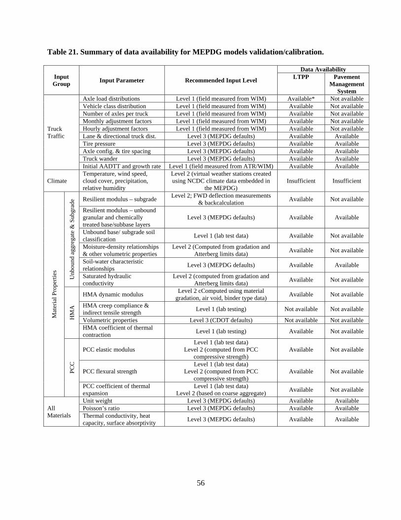
56

Table 21. Summary of data availability for MEPDG models validation/calibration.

Input Group

Input Parameter Recommended Input Level

Data Availability LTPP Pavement

Management System

Truck Traffic

Axle load distributions Level 1 (field measured from WIM) Available* Not available Vehicle class distribution Level 1 (field measured from WIM) Available Not available Number of axles per truck Level 1 (field measured from WIM) Available Not available Monthly adjustment factors Level 1 (field measured from WIM) Available Not available Hourly adjustment factors Level 1 (field measured from WIM) Available Not available Lane & directional truck dist. Level 3 (MEPDG defaults) Available Available Tire pressure Level 3 (MEPDG defaults) Available Available Axle config. & tire spacing Level 3 (MEPDG defaults) Available Available Truck wander Level 3 (MEPDG defaults) Available Available Initial AADTT and growth rate Level 1 (field measured from ATR/WIM) Available Available

Climate Temperature, wind speed, cloud cover, precipitation, relative humidity

Level 2 (virtual weather stations created using NCDC climate data embedded in

the MEPDG) Insufficient Insufficient

Mat

eria

l Pro

pert

ies

Unb

ound

agg

rega

te &

Sub

grad

e Resilient modulus – subgrade Level 2; FWD deflection measurements

& backcalculation Available Not available

Resilient modulus – unbound granular and chemically treated base/subbase layers

Level 3 (MEPDG defaults) Available Available

Unbound base/ subgrade soil classification

Level 1 (lab test data) Available Not available



Available Not available

Soil-water characteristic relationships


Saturated hydraulic conductivity

Level 2 (computed from gradation and Atterberg limits data)


HM

A

HMA dynamic modulus Level 2 cComputed using material

gradation, air void, binder type data) Available Not available


Level 1 (lab testing) Not available Not available

Volumetric properties Level 3 (CDOT defaults) Not available Not available HMA coefficient of thermal contraction

Level 1 (lab testing) Available Not available

PC

C

PCC elastic modulus Level 1 (lab test data)

Level 2 (computed from PCC compressive strength)


PCC flexural strength Level 1 (lab test data)



PCC coefficient of thermal expansion

Level 1 (lab test data) Level 2 (based on coarse aggregate)


All Materials

Unit weight Level 3 (MEPDG defaults) Available Available Poisson’s ratio Level 3 (MEPDG defaults) Available Available Thermal conductivity, heat capacity, surface absorptivity


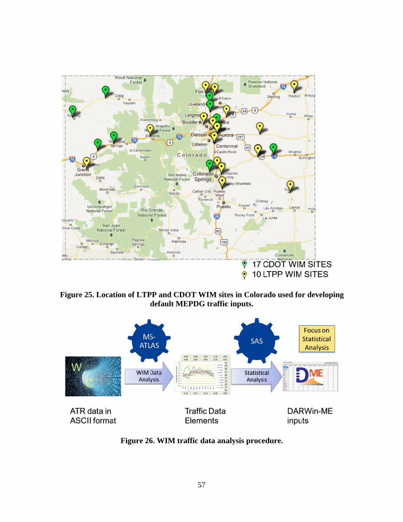
Figu

re 25. Locattion of LTPd

Figure 26

PP and CDOdefault ME

6. WIM traf

57

OT WIM sitPDG traffic

ffic data ana

tes in Colorac inputs.

alysis proce

ado used fo

edure.

r developin

ng

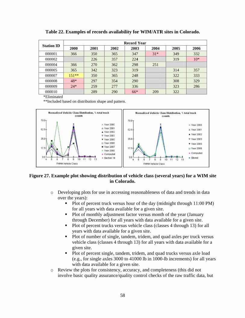
T

St

00000000

*E**

Figure 2

Table 22. E

ation ID

000001 000002 000004 000005 000007 000008 000009 000010 Eliminated *Included base

27. Example

o Develover t

o Revieinvolv

xamples of

2000 2366 3

2366 2365 3

151** 348* 224* 2

2

ed on distributi

e plot showin

loping plots the years):

Plot of perfor all yearPlot of mothrough DPlot of peryears withPlot of numvehicle clagiven site.Plot of per(e.g., for swith data a

w the plots fve basic qual

records ava

2001 20350 36226 35270 36342 32350 36297 35259 27289 29

ion shape and p

ng distributin

for use in ac

rcent truck vrs with data

onthly adjustecember) forcent trucks h data availabmber of singass (classes 4 rcent single, ingle axles 3available forfor consistenlity assuranc

58

ailability for Record Y

02 200365 34757 22462 29823 31965 24854 29077 33690 66*

pattern.

tion of vehicColorado.

ccessing reas

versus hour oavailable fo

tment factor r all years wversus vehicble for a givegle, tandem, 4 through 13

tandem, trid3000 to 4100r a given sitency, accuracce/quality co

r WIM/ATR

Year 3 20047 31*4 8 2519 8 0 6 * 209

cle class (se

sonableness

of the day (mor a given sit

versus montwith data avacle class (claen site. tridem, and

3) for all yea

dem, and qua00 lb in 1000e. y, and comp

ontrol checks

R sites in Co

2005 349 319

314 322 308 323 322

veral years)

of data and

midnight throte. th of the yea

ailable for a gasses 4 throu

quad axles pars with data

ad trucks ve0-lb increme

pleteness (this of the raw

olorado.

2006 332 10*

357 333 329 286

) for a WIM

trends in dat

ough 11:00 P

ar (January given site.

ugh 13) for a

per truck vera available fo

rsus axle loaents) for all y

is did not traffic data,

M site

ta

PM)

all

rsus or a

ad years

but

59

rather a check of MEPDG computed traffic inputs). Examples of the checks that were done are as follows: Whether hourly truck distribution factors add up to 100 percent or if

monthly adjustment factors add up to 12. Occurrences of long zero or “flat” periods in the monthly adjustment or

hourly distribution data (several months or hours with no data). Whether plots of axle loads versus percentage of all axles display distinct

peaks as expected, and whether the percentage of all axles of a given axle type adds up to 100.

Was there consistency in trends over the years with data? Process the raw data using MS-ATLAS to obtain normalized vehicle class distribution,

normalized axle load spectra by class, axle per class coefficients, base year truck volume and annual growth, monthly truck volume adjustment coefficients, and hourly truck volume distribution.

Develop default MEPDG traffic inputs for Colorado sites by identifying natural groupings or clusters for various traffic data elements through statistical cluster analysis—across highway functional class (interstates or U.S. routes), highway location (urban or rural), geographic regions, and so on. Compare Colorado traffic with the MEPDG national defaults and finalize default inputs.

The main objective of traffic data analysis was to (1) determine how representative available traffic data are for pavement design in Colorado using the MEPDG, (2) detect natural groupings or clusters within the available traffic data, and (3) develop defaults for Level 2/3 MEPDG traffic inputs for pavement design. Satisfying the project objectives required performing statistical analysis to determine natural clusters within the traffic and the optimum number of clusters. Natural clusters within the large Colorado traffic data assembled were determined using statistical multivariate hierarchical cluster analysis. Multivariate hierarchical cluster analysis is a statistical procedure used to group “like” observations together when the underlying structure of the data is unknown. Hierarchical cluster analysis consists of either a series of successive divisions of the assembled traffic data set, which is for analysis considered a single cluster, or a merger of data from individual sites to form a single cluster. The divisions or mergers are done according to their similarities in the individual data sets. The similarities are based on distances between individual data sets of clusters within the larger database. Thus, cluster analysis begins with grouping individual sites with the smallest distances between them to form the first set of clusters. Next, the individual sites with the next smallest distances between them and the clusters are added to the original set of clusters. This continues until all individual observations and clusters end up together in one large group. Although clusters can be developed using a variety of different methods, all the methods available apply some measure of distance between observations as a basis for creating clusters. Since the cluster analysis methodology does not require prior knowledge of the number of clusters with a given set of data, it is critical that a procedure be applied to determine the optimum number of clusters within the database being analyzed. There is no clear-cut method for determining the optimum number of clusters within a data set. Thus, analysts must depend on a combination of diagnostic statistics to determine the optimum number of clusters. Although

several suin determpartial sq(PSF), an

Vehicle C Figure 28CDOT ve

Cfo

Cru

Ctwur

Vehicle c

F

uch statisticsmining optimquared multipnd pseudo t2

Class Distrib

8 presents anehicle class

Cluster 1: Priour-lane rura

Cluster 2: Priural principa

Cluster 3: Twwo-lane rurarban princip

class distribu

Figure 28. E

s are availabmum number

ple correlati(PST2).

bution

n example ofdistributions

imary peak fal principal aimary peak fal arterial-Intwo distinct peal major collepal arterial.

utions of the

Example of

ble, for this sof clusters: on (R2), eige

f the outputss belong to t

for class 5. Sarterial-otherfor class 9. Sterstate. eaks for clasectors, two-l

e three CDOT

the outputs

60

study, five dicubic clusteenvalue and

s obtained frhree groupin

Smaller peakr.

Smaller peak

sses 5 and 9. lane rural pri

T clusters ar

s obtained fr

iagnostic staering criterio

associated v

rom statisticangs that can

ks for class 8

ks for class 5

Smaller pearincipal arter

re presented

rom statisti

atistics were on (CCC), cuvariance (VA

al cluster anabe described

8 & class 9. P

. Primarily f

aks for classrial-other, an

in Figure 29

cal cluster a

selected forumulative anAR), pseudo

alysis. The d as follows

Primarily for

for four-lane

8. Primarilynd four-lane

9.

analysis.

r use nd F

:

r

e

y for

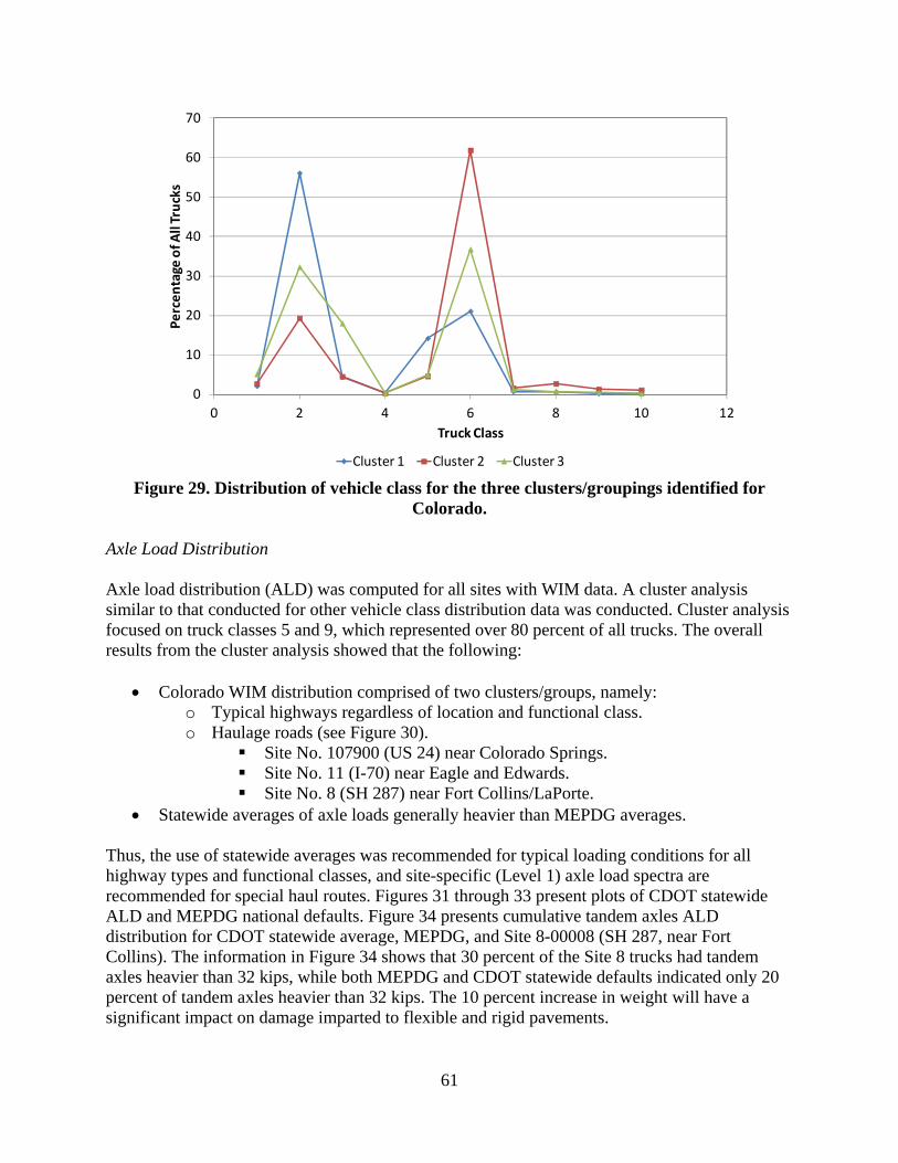
61

Figure 29. Distribution of vehicle class for the three clusters/groupings identified for

Colorado. Axle Load Distribution Axle load distribution (ALD) was computed for all sites with WIM data. A cluster analysis similar to that conducted for other vehicle class distribution data was conducted. Cluster analysis focused on truck classes 5 and 9, which represented over 80 percent of all trucks. The overall results from the cluster analysis showed that the following:

Colorado WIM distribution comprised of two clusters/groups, namely: o Typical highways regardless of location and functional class. o Haulage roads (see Figure 30).

Site No. 107900 (US 24) near Colorado Springs. Site No. 11 (I-70) near Eagle and Edwards. Site No. 8 (SH 287) near Fort Collins/LaPorte.

Statewide averages of axle loads generally heavier than MEPDG averages. Thus, the use of statewide averages was recommended for typical loading conditions for all highway types and functional classes, and site-specific (Level 1) axle load spectra are recommended for special haul routes. Figures 31 through 33 present plots of CDOT statewide ALD and MEPDG national defaults. Figure 34 presents cumulative tandem axles ALD distribution for CDOT statewide average, MEPDG, and Site 8-00008 (SH 287, near Fort Collins). The information in Figure 34 shows that 30 percent of the Site 8 trucks had tandem axles heavier than 32 kips, while both MEPDG and CDOT statewide defaults indicated only 20 percent of tandem axles heavier than 32 kips. The 10 percent increase in weight will have a significant impact on damage imparted to flexible and rigid pavements.

0

10

20

30

40

50

60

70

0 2 4 6 8 10 12

Percentage of A

ll Trucks

Truck Class

Cluster 1 Cluster 2 Cluster 3

Figure 3

F

FractionofSingleAxles

inaLoadGroup

30. ExampleALD when

igure 31. St

0

2

4

6

8

10

12

14

16

18

20

Fraction of Single Axles in

a Load Group

es of location compared

tatewide and

on of speciald to other lo

d national A

62

l haulage rocations with

ALD for sin

Axle load,

oads showinhin the state

ngle axles of

Ibs

C

C

D

D

ng significane highway s

f class 5 and

DOT Class 5

DOT Class 9

DARWin‐ME C

DARWin‐MEC

nt differencesystem.

d 9 trucks.

Class 5

Class 9

es in

Figure

FractionofTandem

Axles

inaLoad

Group

Figure 32.

e 33. CDOT

0

2

4

6

8

10

12

14

Fraction of Tandem Axles in a Load

Group

Statewide a

T statewide a

and nationa

average, ME

63

al ALD for t

EPDG, and

Axle Load,

tandem axle

d Site 8-0000

, Ibs

CDOT

CDOT

DARW

DARW

es of class 6

08 ALD for

T Class 6

T Class 9

Win‐ME Clas

Win‐ME Clas

6 and 9.

tandem axl

ss 6

ss 9

les.

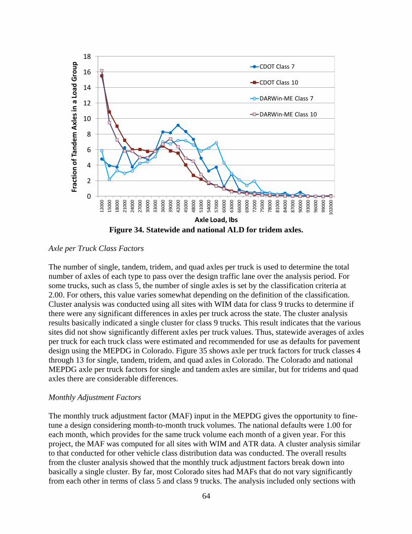
64

Figure 34. Statewide and national ALD for tridem axles.

Axle per Truck Class Factors The number of single, tandem, tridem, and quad axles per truck is used to determine the total number of axles of each type to pass over the design traffic lane over the analysis period. For some trucks, such as class 5, the number of single axles is set by the classification criteria at 2.00. For others, this value varies somewhat depending on the definition of the classification. Cluster analysis was conducted using all sites with WIM data for class 9 trucks to determine if there were any significant differences in axles per truck across the state. The cluster analysis results basically indicated a single cluster for class 9 trucks. This result indicates that the various sites did not show significantly different axles per truck values. Thus, statewide averages of axles per truck for each truck class were estimated and recommended for use as defaults for pavement design using the MEPDG in Colorado. Figure 35 shows axle per truck factors for truck classes 4 through 13 for single, tandem, tridem, and quad axles in Colorado. The Colorado and national MEPDG axle per truck factors for single and tandem axles are similar, but for tridems and quad axles there are considerable differences. Monthly Adjustment Factors The monthly truck adjustment factor (MAF) input in the MEPDG gives the opportunity to fine-tune a design considering month-to-month truck volumes. The national defaults were 1.00 for each month, which provides for the same truck volume each month of a given year. For this project, the MAF was computed for all sites with WIM and ATR data. A cluster analysis similar to that conducted for other vehicle class distribution data was conducted. The overall results from the cluster analysis showed that the monthly truck adjustment factors break down into basically a single cluster. By far, most Colorado sites had MAFs that do not vary significantly from each other in terms of class 5 and class 9 trucks. The analysis included only sections with

0

2

4

6

8

10

12

14

16

18

12000

15000

18000

21000

24000

27000

30000

33000

36000

39000

42000

45000

48000

51000

54000

57000

60000

63000

66000

69000

72000

75000

78000

81000

84000

87000

90000

93000

96000

99000

102000

Fraction of Tandem

Axles in a Load

Group

Axle Load, Ibs

CDOT Class 7

CDOT Class 10

DARWin‐ME Class 7

DARWin‐ME Class 10

65

all 12 months MAF. Thus, MAFs from all sites were used to develop statewide averages and defaults. The default MAFs for class 5 and 9 trucks are presented in Figure 36. Hourly Truck Volume Distribution Hourly truck distribution data over 24 hours are available for most of the ATR and WIM sites. Cluster analysis was performed to determine whether the hourly truck distributions from the sites located throughout the state belonged to a single or multiple grouping. Potential groupings were investigated by geographical location, functional class, and so on. The results of the analysis showed a single grouping for the entire state, as location, functional class, etc., had no significant impact on the distributions. Thus, a single statewide default hourly truck volume distribution was developed; see Figure 37. The CDOT default hourly truck volume distribution was similar to the MEPDG national default.

Figure 35. Statewide and national MEPDG averages for axle per trucks.

0.0

0.5

1.0

1.5

2.0

2.5

3.0

3.5

4.0

4.5

5.0

VC4

VC5

VC6

VC7

VC8

VC9

VC10

VC11

VC12

VC13

Number of A

xles Per Truck

Single Axle

0.0

0.5

1.0

1.5

2.0

2.5

VC4

VC5

VC6

VC7

VC8

VC9

VC10

VC11

VC12

VC13

Number of A

xles Per Truck

Tandem Axle

0.0

0.1

0.2

0.3

0.4

0.5

0.6

0.7

0.8

0.9

1.0

VC4

VC5

VC6

VC7

VC8

VC9

VC10

VC11

VC12

VC13

Tridem Axle

0.000

0.005

0.010

0.015

0.020

0.025

0.030

0.035

0.040

0.045

VC4

VC5

VC6

VC7

VC8

VC9

VC10

VC11

VC12

VC13

Quad Axle

66

Figure 36. Statewide averages and default MAFs for class 5 and 9 trucks.

Figure 37. CDOT statewide averages and MEPDG default hourly truck volume

distribution.

0

0.2

0.4

0.6

0.8

1

1.2

1.4

0 2 4 6 8 10 12 14

Truck Class

Class 5 Class 9

0.0

1.0

2.0

3.0

4.0

5.0

6.0

7.0

8.0

12:00 AM

1:00 AM

2:00 AM

3:00 AM

4:00 AM

5:00 AM

6:00 AM

7:00 AM

8:00 AM

9:00 AM

10:00 AM

11:00 AM

12:00 PM

1:00 PM

2:00 PM

3:00 PM

4:00 PM

5:00 PM

6:00 PM

7:00 PM

8:00 PM

9:00 PM

10:00 PM

11:00 PM

Fraction of Trucks in a given

Hour of the Day

67

Estimating Missing Climate Data Assessing Climate Data Availability The MEPDG contained 20 Colorado weather stations for use in developing virtual pavement location/site specific climate data for design and analysis. Another 8 to 10 weather stations in neighboring states (Utah, Wyoming, Nebraska, Kansas, Oklahoma, New Mexico, Arizona) could be used in creating virtual weather stations in Colorado’s border regions. Table 23 contains a summary list of the weather stations included in the MEPDG for Colorado, and Figure 38 shows their locations across the state. A review of the MEPDG default Colorado weather stations indicated the following:

On average, the weather stations contained 10 years of data. There was considerable distance between the weather stations. Increasing the distance

between weather stations does negatively impact the accuracy of virtual weather stations created for pavement design.

Thirteen of the 20 weather stations were located in elevations < 6000 ft. Only one weather station was located in a region with elevation greater than 8500 ft. The remaining weather stations were located in regions with elevation between 6000 and 8500 ft. This implied that higher elevations (very cold and cold climate zones) were under-represented.

Some of the weather stations reported gaps in available data.

Table 23. Summary list of weather stations included in the MEPDG for Colorado.

City Airport Longitude, deg Latitude, deg Elevation, ft Akron Colorado Plains Regional Airport 40.1 -103.14 4664

Alamosa San Luis Valley Regional Airport 37.26 -105.52 7536 Aspen Aspen-Pitkin County Airport 39.13 -106.52 7725

Burlington Kit Carson County Airport 39.14 -102.17 4198 Colorado Springs

City of Colorado Springs Municipal Airport 38.49 -104.43 6183

Cortez Cortez Municipal Airport 37.18 -108.38 5899 Craig Craig-Moffat Airport 40.3 -107.31 6192

Denver Denver International Airport 39.5 -104.4 5382 Denver Centennial Airport 39.34 -104.51 5827

Durango Dura-La Plata County Airport 37.08 -107.46 6677 Grand Junction Walker Field Airport 39.08 -108.32 4826

La Junta La Junta Municipal Airport 38.03 -103.32 4193 Lamar Lamar Municipal Airport 38.04 -102.41 3675

Leadville Leadville/Lake County Airport 39.14 -106.19 9938 Limon Limon Municipal Airport 39.11 -103.43 5350 Meeker Meeker Airport 40.03 -107.53 6333

Montrose Montrose Regional Airport 38.31 -107.54 5753 Pueblo Pueblo Memorial Airport 38.17 -104.3 4655 Rifle Garfield County Regional Airport 39.32 -107.44 5506

Trinidad Perry Stokes Airport 37.16 -104.2 5749

F Thereforminimum

A Q

d A

co Identifica Updatingin the staidentifiedFigure 39stations aprecipitatcooperatichecks.

Figure 38. L

e, it was necm:

Additional daQuality assur

ata/trends anAdditional weonditions.

ation of Add

g and augmeate with the dd all signific9 shows the are mostly option. The Naive stations d

Locations of

cessary to up

ata as availabrance/qualitynd to fill ideneather statio

ditional Weat

nting Coloradata types reant weather locations of perated by loational Weatdata sets and

f Colorado w

pdate and aug

ble (i.e., misy control (QAntified gaps ns to better c

ther Stations

ado MEPDGequired for th

stations in thf selected cooocal observether Service d subjects th

68

weather sta

gment the C

sing years).A/QC) on avin data. characterize

s

G climate dathe MEPDG. he state, incloperative staers and repor(NWS) inclue data to ext

ations includ

Colorado wea

vailable data

e and represe

ta began by This was doluding coopations in Colrt maximumudes other ptensive autom

ded in the M

ather station

a to assure re

ent Colorado

identifying wone through erative weatlorado. Thes

m/minimum tepertinent infomated and m

MEPDG.

s to include,

easonablenes

o climate

weather statiCDOT, whi

ther stations.se weather emperaturesormation in

manual QC

, as a

ss of

ions ich .

s and

Figur

Criteria ffollows:

Mp

M M M

An efficiclimate dstations cleading toreview ofof data. Ainto the Midentified Developm The finaldetailed rrequired raw data,

re 39. Locat

for selecting

Must contain ercent cloud

Must contain Must be locatMust contain

ient and consdata files. Thclimate data o the selectiof data contaiAll weather sMEPDG. Bad for use in d

ment of MEP

l step in updreview of allby the MEP, filling gaps

tions of Colo

additional w

all climate dd cover, prec

a minimumted in an unrgood quality

sistent methohe methodolofrom CDOTon of projecined in the cstations with

ased on the cdeveloping v

PDG Climate

ating and aul selected we

PDG (i.e., HCs in the data,

orado weathcooper

weather stati

data elementipitation, wi

m of 5 years orepresented ry data (in ter

odology wasogy began wT. The locatits located inlimate data s

h reasonable criteria presevirtual weath

e Files for A

ugmenting theather stationCD file form and transfor

69

her stationsrative statio

ons to augm

ts required bind speed). of data. region/area.rms of both

s designed towith obtainin

ons of the Nn regions/aresets to determdata availab

ented above, her stations i

Additional Co

he CDOT MEns’ climate d

mat). Transforming data i

s included inons.

ment the MEP

by the MEPD

data elemen

o update the ng selected CNWS coopera

as of interesmine the avable were flagan additiona

in Colorado.

olorado Wea

EPDG climadata and tran

ormation of dinto the units

n the MEPD

PDG default

DG (tempera

nt magnitude

Colorado wColorado NWative stationst. Next was ailability andgged for posal 22 weathe

ather Station

ate data was nsform the ddata includeds of measure

DG and NW

ts were as

ature, humid

e and trends)

weather statioWS cooperatins were revie

a preliminard reasonablesible inclusier stations w

ns

to conduct adata into the d cleaning upement requir

WS

dity,

).

on ive ewed, ry eness ion

were

a form

up the red

70

by the MEPDG. The procedure utilized for data transformation and creation of HCD files is as follows:

1. Import raw climate data into project climate databases in MS Access format. Note that climate data were reported hourly. The raw data included the following variables as a minimum, reported on an hourly basis:

a. Time stamp (comprised of Year|Month|Day|Hr presented as a string). b. Ambient temperature in degrees F. c. Wind speed, in miles per hour. d. Percent sunshine or cloud cover (percentage). e. Precipitation in inches. f. Humidity as a percentage.

2. Conduct basic QC of raw climate data. The QC checks were to ensure that the raw climate data fell within the typical ranges provided in Table 24. Raw data that fell outside the typical range was either removed from the data set or had its value capped at the extreme value of the range.

3. Transform time stamp to Year|Month|Day|Hr into a unique date/hour. 4. Round reported time to the nearest hour (e.g., 9:57 AM becomes 10:00HRS and 9:57 PM

becomes 22:00HRS) and then transform to MEPDG format for hours (e.g., 10:00 becomes 10 while 22:00 becomes 22).

5. Determine mean hourly climate values on an annual basis (i.e., for each combination of Month|Day|Hr, determine average temperature, wind speed, percent sunshine, precipitation, and humidity).

6. Determine earliest reporting date/time (e.g., 10:00 January 16, 1957). 7. Determine latest reporting date/time (e.g., 16:34 June 26, 2007). 8. Establish climate file start/end (e.g., 00:00 January 1, 1957, to 23:00 December 31,

2007). 9. Generate hourly time stamp for the period between the start and end dates established in

step 8. Call this the baseline HCD file. See example below in Table 25. 10. Using the hourly time stamp for the period between the start and end dates established in

step 9 as reference, determine all the hours within the start and end dates with and without climate data. For hours with data, assume the data values reported in the climate data sets have undergone QA/QC checks. For all hours with missing data, assume the mean values computed in step 5.

11. Recheck the hourly time stamp for the period between the start and end dates established in step 9 to determine if there are still hours with missing data (i.e., hours for which average values are not available). For this situation, apply statistical algorithms (interpolation/extrapolation based on assumed distribution of climate data variable [e.g., normal, beta, and log-normal]) to determine best estimate of missing data.

12. Use the climate data set developed in steps 9 through 11 to develop HCD files. 13. Update MEPDG station.dat file to enable MEPDG to read in new HCD files 14. Test HCD files using MEPDG interface to determine reasonableness of data entries

(MEPDG will flag outliers and erroneous data inputs). 15. Revise HCD files as needed based on MEPDG outcomes 16. Prepare final files and include in MEPDG database for Colorado.

Dat

195701957019570

20072007

The da Figure 40Colorado.methodoloincluded tMEPDG f

Table 24. T

Climate

TemperWind spPercent

PrecipRelative

Table 2

te/Hr T

010100 010101 010102

123122 123123 ate and hour ha

shows the lo. Figures 41 thogy presentedto replace misfor Colorado.

Figure 40.

Typical clim

Variable

rature, °F eed, mph sunshine

pitation humidity

25. Baseline

Temp, °F W

ave been merge

ocations of MEhrough 45 pred above. The ssing data. Ta.

Map showin

mate data ra

e time stamp

Wind Speed, m

ed to provide r

EPDG and CDesent plots ofplots show cl

able 26 presen

ng location

71

anges used i

Minimum-100

0 0 0 0

p for MEPD

mph Sunsperc

reference date/h

DOT climate f MEPDG climlearly the orignts a summary

of MEPDG

in conductin

Ranm

DG HCD file

shine, cent

Pre

hr in column 1

stations inclumate data varginal climate y of weather

G and CDOT

ng QA/QC c

nge M

e developme

ecipitation, in

1.

uded in the Mriables develodata availablestations inclu

T weather s

checks.

Maximum 150 100 100 10 100

ent.

Humidipercen

MEPDG for oped using thee and estimat

uded in the

tations.

ity, nt

e tes

72

Figure 41. Plot showing reported (blue ddot) and estima

ated (red star) t

temperature daata for HCD fille 31013 in Col

lorado.

73

Figure 42. Plot showing rreported (blue dot) and estim

ated (red star)

wind speed daata for HCD filee 31013 in Colo

orado.

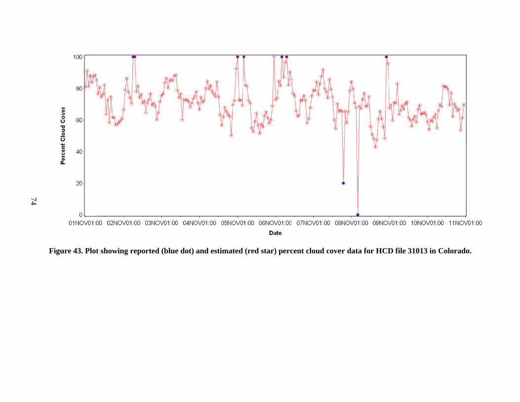
74

Figure 43. Plott showing reporrted (blue dot) and estimated

(red star) perccent cloud coveer data for HCDD file 31013 in

Colorado.

75

Figure 444. Plot showingg reported (bluue dot) and estim

mated (red star

r) rainfall dataa for HCD file 331013 in Colora

ado.

76

Figure 45. Ploot showing reported (blue dott) and estimated

d (red star) rellative humidityy data for HCDD file 31013 in C

Colorado.

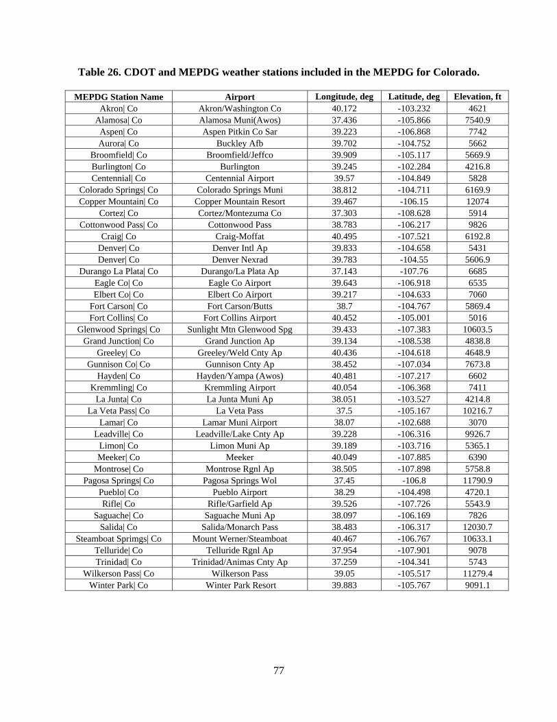
77

Table 26. CDOT and MEPDG weather stations included in the MEPDG for Colorado.

MEPDG Station Name Airport Longitude, deg Latitude, deg Elevation, ft Akron| Co Akron/Washington Co 40.172 -103.232 4621

Alamosa| Co Alamosa Muni(Awos) 37.436 -105.866 7540.9 Aspen| Co Aspen Pitkin Co Sar 39.223 -106.868 7742 Aurora| Co Buckley Afb 39.702 -104.752 5662

Broomfield| Co Broomfield/Jeffco 39.909 -105.117 5669.9 Burlington| Co Burlington 39.245 -102.284 4216.8 Centennial| Co Centennial Airport 39.57 -104.849 5828

Colorado Springs| Co Colorado Springs Muni 38.812 -104.711 6169.9 Copper Mountain| Co Copper Mountain Resort 39.467 -106.15 12074

Cortez| Co Cortez/Montezuma Co 37.303 -108.628 5914 Cottonwood Pass| Co Cottonwood Pass 38.783 -106.217 9826

Craig| Co Craig-Moffat 40.495 -107.521 6192.8 Denver| Co Denver Intl Ap 39.833 -104.658 5431 Denver| Co Denver Nexrad 39.783 -104.55 5606.9

Durango La Plata| Co Durango/La Plata Ap 37.143 -107.76 6685 Eagle Co| Co Eagle Co Airport 39.643 -106.918 6535 Elbert Co| Co Elbert Co Airport 39.217 -104.633 7060

Fort Carson| Co Fort Carson/Butts 38.7 -104.767 5869.4 Fort Collins| Co Fort Collins Airport 40.452 -105.001 5016

Glenwood Springs| Co Sunlight Mtn Glenwood Spg 39.433 -107.383 10603.5 Grand Junction| Co Grand Junction Ap 39.134 -108.538 4838.8

Greeley| Co Greeley/Weld Cnty Ap 40.436 -104.618 4648.9 Gunnison Co| Co Gunnison Cnty Ap 38.452 -107.034 7673.8

Hayden| Co Hayden/Yampa (Awos) 40.481 -107.217 6602 Kremmling| Co Kremmling Airport 40.054 -106.368 7411

La Junta| Co La Junta Muni Ap 38.051 -103.527 4214.8 La Veta Pass| Co La Veta Pass 37.5 -105.167 10216.7

Lamar| Co Lamar Muni Airport 38.07 -102.688 3070 Leadville| Co Leadville/Lake Cnty Ap 39.228 -106.316 9926.7

Limon| Co Limon Muni Ap 39.189 -103.716 5365.1 Meeker| Co Meeker 40.049 -107.885 6390

Montrose| Co Montrose Rgnl Ap 38.505 -107.898 5758.8 Pagosa Springs| Co Pagosa Springs Wol 37.45 -106.8 11790.9

Pueblo| Co Pueblo Airport 38.29 -104.498 4720.1 Rifle| Co Rifle/Garfield Ap 39.526 -107.726 5543.9

Saguache| Co Saguache Muni Ap 38.097 -106.169 7826 Salida| Co Salida/Monarch Pass 38.483 -106.317 12030.7

Steamboat Sprimgs| Co Mount Werner/Steamboat 40.467 -106.767 10633.1 Telluride| Co Telluride Rgnl Ap 37.954 -107.901 9078 Trinidad| Co Trinidad/Animas Cnty Ap 37.259 -104.341 5743

Wilkerson Pass| Co Wilkerson Pass 39.05 -105.517 11279.4 Winter Park| Co Winter Park Resort 39.883 -105.767 9091.1

78

CHAPTER 5. DEVELOPMENT OF MATERIALS DATABASE FOR MEPDG MODEL VALIDATION/CALIBRATION This chapter describes work done to develop a materials database for use in MEPDG model calibration/validation. Developing the CDOT MEPDG materials input database began with a detailed description of all required MEPDG materials data inputs, along with a summary of data availability (see Table 27). Table 27 shows a significant lack of HMA, PCC, and unbound aggregate materials input data for most CDOT pavement management system projects and some LTPP projects. This was as expected, as projects in pavement management system databases typically do not contain such detailed information.

Table 27. Summary of data availability for MEPDG models validation/calibration.

Input Group

Input Parameter Recommended Input Level Data Availability

LTPP CDOT

Mat

eria

l Pro

pert

ies

Unb

ound

agg

rega

te

& S

ubgr

ade

Resilient modulus – subgrade Level 2 (FWD deflection measurements

& backcalculation) Available Not available

Unbound base/subgrade soil classification

Level 1 (lab test data) Available Not available




Saturated hydraulic conductivity



HM

A

HMA dynamic modulus Level 1 (Testing for a range of

temperatures and load frequencies) Not available Not available


Level 1 (Testing for a range of temperatures and load frequencies)

Not available Not available

Volumetric properties Level 3 (CDOT defaults) Not available Not available HMA coefficient of thermal contraction

Level 1 (lab testing) Not available Not available

PC

C

PCC elastic modulus Level 1 (lab test data)



PCC flexural strength Level 1 (lab test data)



PCC CTE Level 1 (lab test data)

Level 2 (based on coarse aggregate) Available Not available

Next, the project team reviewed CDOT pavement design and construction records to determine material data available in CDOT QA/QC databases for use in developing default material inputs. Note that default material inputs are not project-specific material property values but rather Level 3 statewide defaults estimated from tests conducted on similar materials with similar property values. The outcome of the data availability checks and records review was used as the basis for developing a comprehensive field/laboratory forensic evaluation, laboratory testing, and

79

construction records and QA/QC data review program. The program consisted of the following steps:

1. Construction records and CDOT pavement project QA/QC data review. o Identification of typical CDOT paving materials.

HMA and asphalt treated material. PCC. Chemically treated materials. Unbound granular (base/subbase) materials. Subgrade soils.

o Identification of pertinent materials data available in QA/QC databases. Gradation. Strength. Modulus. Asphalt binder type, content, and volumetrics. PCC CTE.

2. Refinement of data needs (revise information in Table 27 to reflect data available in CDOT materials QA/QC databases) and development of list of missing project specific or statewide (Level 3) data.

3. Development of field/laboratory test program to acquire missing data. o Identification of material sources (laboratory or field destructive/nondestructive

testing locations). o Identification of test protocols and equipment needs. o Development of testing schedule.

4. Performance of field/laboratory testing and development of test database. 5. Evaluation of test data for accuracy and reasonableness. 6. Development of default MEPDG inputs.

The research team implemented this plan with assistance from CDOT. The following sections present a detailed description of the plan implementation and outcomes. Construction Records and CDOT Pavement Projects QA/QC Data Review For the identified missing data, only as-placed HMA air voids and binder content data were available in the CDOT QA/QC databases. These data were extracted and assembled for inclusion in the project materials database. Laboratory/Field Testing With the review of CDOT materials databases completed, the only feasible means of obtaining the remaining missing data was through laboratory/field testing. Details are presented in the following sections.

Extractio Forty pavperformepavemenprojects sthe field

Figure 4

on, Examinat

vement projeed on the 16 nt project siteselected for testing layou

Figure 46.

47. Schemat

Start 0 ft

200''

A

tion, and Lab

ects were idenew HMA p

es, and 3 HMfield testing ut for each s

Map of the

tic showing

Station:

Right Wheelp

G

A

MATEFLEXIBL

Number of C

boratory Tes

entified for fpavement pr

MA overlay oare presente

selected proj

locations of

the outline along with

Location of Cores over ALongitudinal cracks in t Locations of Cores for HSamples for Moisture CClassification of Unbou Locations of Cores for H

Location of Cores for Hfrom the Left Wheelpath

400'

ath

B

Left Wheelpath

ERIALS SAMPLINLE PAVEMENTS

Sampling and F

Cores = 6 (8 if wheelpat

80

sting of Core

field testing.roject sites, 2over existinged in Figure ect.

f the 40 pro

of the field h coring pat

Alligator or he Wheelpath (located as n

HMA Air Void & other HMontent Tests of Unbound Mnd and Soil Materials

HMA Air Void & other HM

HMA Rut Depth Determinath)

60

H

E

NG & FIELD TESS PROJECTS – NO

Field Testing Pla

th longitudinal cracking

es

. Specifically21 HMA oveg JPCP proje46. Figure 4

ojects selecte

d testing plantterns.

eeded in either wheelpath).

MA Laboratory Tests and AuMaterials and Soils and Visu

MA Laboratory Tests

ion (one from the Right and

00'

Between Wheelp

F

C

STING PLAN FORON-LTPP SECTIO

an Layout

g or alligator cracking e

y, field testinerlay over exect sites. The47 presents a

ed for field

n for each s

uger ual

d one

End Station: 1,000 ft

800'

paths

D

R ONS

exists)

ng was xisting HMAe locations oa schematic

testing.

selected pro

A of the of

ject,

81

Field testing essentially consisted of HMA coring and extraction of HMA/PCC cores and unbound aggregate base and subgrade soil samples. The extracted cores were examined and tested for basic volumetric, strength, thickness, and durability properties. Other laboratory/field testing performed included layer thickness measurements, trenching, distress surveys, and rut depth measurements. A photographic journal of the extracted cores was created and used throughout the project as a visual identification of the pavement and material condition. Photos were also taken to document the condition of the pavement in the area of sampling, and the location of the sampling with reference to the lane and wheel path. Photos of the coring process and core extraction was kept for use in interpreting laboratory results. The key elements of the field/laboratory test program were as follows:

Identification and marking of the 1000-ft sampling area within each project site. Identification and marking coring of locations and extraction of cores.

o Between wheel paths (lane center). Four 6-in-diameter HMA cores were extracted. Hand augers were used at the four core locations to extract base/subgrade materials. The sampled material was sealed in plastic bags and labeled.

o Within 12-in left/right wheel path. Four 6-in-diameter HMA cores were extracted. o The extracted cores were labeled, photographed, and logged in the field. Core

holes were patched with either cold patch mix or rapid set mortar to match pavement type.

Examination and laboratory testing of extracted cores. o All cores were checked for debonding from the original pavement and signs of

stripping, moisture damage, etc. o The 6-in HMA cores extracted from the lane center were tested to determine

HMA layer thickness and to determine as-placed HMA air voids, volumetric binder content, gradation, bulk specific gravity, and maximum theoretical specific gravity (“Rice” density).

o Atterberg limits, sieve analysis (gradation), and in situ moisture content tests were determined for the extracted unbound aggregate and subgrade soil materials. Results were used to determine base/subgrade materials type (i.e., AASHTO soil class) and in situ moisture content.

o The four HMA cores extracted from within the wheel path were examined to determine the amount of rutting within HMA layers and to determine whether longitudinal wheel path cracks were top-down fatigue (longitudinal) or bottom-up fatigue (alligator) cracking.

Figures 48 through 50 present photos/schematics of various aspects of the field testing program. Table 28 presents a summary of information derived from the coring effort (HMA air voids and volumetric binder content), and Figures 51 and 52 show the distribution of HMA air voids and volumetric binder content, respectively.

Figuree 48. Sampl

Figu

ling section

ure 49. Pave

layout, core

ement coring

82

e locations,

g rig used fo

and sample

or materials

e of extracte

s extraction

ed HMA cor

n.

re.

Tab

Sectio

04-9105-1205-1207-1307-1308-1209-1310-1211-1212-1314-1315-1116-1317-1320-1321-91

F

ble 28. Summ

on ID C

1044 2441 2441 D3817 A3817 2685 3969 2393 2529 3390 3131 1959 3440 3932 3353 1094

Figure 50. E

mary of extr

Core ID

F D-top

D-bottom A-bottom

A-top E B F F B C C A F C A

Example of f

racted HMA

Binder

PG 58-40AC-20

Pen 85-100Pen 85-100PG 64-28PG 64-22PG 64-22PG 64-28PG 64-22PG 64-22PG 58-28PG 58-28PG 64-22PG 64-28PG 76-28PG 64-22

83

field logging

A cores air v

As-consVoid

0 0

g of extracte

voids and b

structed Airs, percent 7.5 5.8 8.6

11.6 5.3 8.0 6.0 5.5 6.5 5.3 6.2 8.0 6.8 6.8 4.5 7.2

ed cores.

binder conte

r As-coBinder

ent test resu

onstructed VContent, p

9.5 11.0 16.1 14.7 12.5 6.3 8.5

17.0 9.6

12.5 13.4 12.4 9.2 9.6

14.6 10.1

ults.

Vol. ercent

84

Table 28. Summary of extracted HMA cores air voids and binder content test results.

Section ID Core ID Binder As-constructed Air

Voids, percent As-constructed Vol.

Binder Content, percent 22-12297 A PG 76-28 8.2 13.5 23-11918 D PG 76-28 6.2 10.6 24-13356 E PG 76-28 6.4 8.6 27-13959 E-middle PG 58-28 3.7 11.4 27-13959 B-top PG 58-34 7.5 7.0 28-11865 B PG 58-28 3.9 9.2 30-11979 C AC-20 5.5 9.0 31-13258 F PG 58-28 5.8 11.2 32-12448 F AC-20 4.4 12.2 33-13435 F PG 58-28 6.8 10.3 34-13513 C PG 58-28 3.2 13.8 35-13087 F PG 58-28 6.5 11.9 36-13880 E PG 58-34 4.5 16.4 37-92976 A PG 58-40 4.5 16.6 38-13505 E PG 58-28 4.8 11.7 39-11970 E PG 58-28 8.2 11.4 41-13325 F PG 76-28 7.4 11.1 42-12153 A PG 76-28 6.6 8.9 43-13085 F PG 58-28 4.1 11.5 44-11213 F PG 58-28 5.9 9.6 45-13106 D PG 64-28 6.2 7.9 47-12018 C PG 58-34 6.5 7.0 48-13866 F PG 64-28 7.8 5.9 49-13864 B PG 64-28 7.9 9.2 50-11780 F PG 58-28 9.8 8.6 51-12271 C PG 58-28 6.6 10.1 52-12321 F PG 64-22 6.9 7.5

MEAN 6.4 10.9

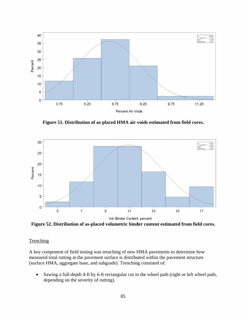
Fi

Figure

Trenchin A key comeasured(surface H

Sd

igure 51. Di

52. Distribu

ng

omponent of d total ruttinHMA, aggre

awing a fullepending on

istribution o

ution of as-p

field testingg at the paveegate base, a

l-depth 4-ft bn the severity

of as-placed

placed volum

g was trenchiement surfacand subgrade

by 6-ft rectany of rutting).

85

d HMA air v

metric bind

ing of new Hce is distribue). Trenching

ngular cut in

voids estima

der content e

HMA pavemuted within thg consisted o

n the wheel p

ated from fi

estimated fr

ments to deterhe pavementof:

path (right or

ield cores.

rom field co

rmine how t structure

r left wheel

ores.

path,

Dd

R P C P

th

B TrenchinGlenwooaspects odistributipresentedpredicted

Figu

Double cuttinamage when

Removal of thartial excava

Complete baslacement of

he straightedo Deptho Measuo Measu

Backfilling of

ng for this prod Springs, aof the trenchiion of total rd in Table 29d total rutting

ure 53. Sawi

ng the trenchn excavated. he sawcut paation of the use excavationf a straighteddge to each ph to each layeurements recurements takf trench and

roject was doand on Coloring operationrutting within9. This inforg within the

ing and liftin

h along the tr

avement. unbound basn by hand an

dge atop the tpavement layer measuredcorded everyken from botplacement o

one at three lrado Boulevans and outcon the pavemrmation will pavement st

ng of surfac

86

ransverse sid

se material.nd cleaning ttrench face ayer as followd from a straiy 3 inches alth sides of thof HMA patc

locations: I-2ard in Denveome in termsent structurebe used in rutructure.

ce HMA lay

des to protec

the trench faand measure

ws: ightedge plaong trench f

he trench forch.

25 near Coloer. Figures 5s of layer proe for the threrutting mode

yer during t

ct the trench

ace. ement of the

aced across toface. r comparison

orado Spring53 through 5ofiles and ruee projects exel calibration

he trenchin

face from

distance fro

op of trench

n.

gs, SH 82 ne6 show vario

ut depth. Thexamined is

n to apportion

ng operation

om

h.

ear ous

e

n

n.

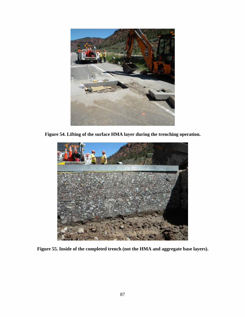
F

Figu

Figure 54. L

ure 55. Insid

Lifting of th

de of the com

e surface H

mpleted tren

87

HMA layer d

nch (not the

during the tr

e HMA and

renching op

aggregate b

peration.

base layers)).

88

Figure 56. Plots of layer profile and rut depth across the 12-ft lane width.

Table 29. Distribution of total rutting (percentage within layer) within the pavement structure.

Layer Type/Material

Projects Mean I-25 (near Colorado

Springs)Glenwood Springs

(SH 82)Colorado

Blvd* HMA surface 70 63 55 63 Aggregate base/subbase

5 9 20 11

Subgrade (top 12 in) 25 28 25 26 *Includes subbase. Nondestructive Deflection Testing CDOT performed FWD testing in a separate effort to obtain deflection test data for use in backcalculating pavement layer moduli and modulus of subgrade reaction for PCC and composite pavements. For all the HMA pavement projects selected, FWD testing was performed in 25-ft intervals. For PCC pavements, FWD testing was performed at slab centers, at transverse joints (to determine load transfer efficiency), and at the slab corners to determine maximum joint deflections.

0

2

4

6

8

10

12

0 6 12 18 24 30 36 42 48 54 60 66 72

Dep

th fr

om S

urf

ace,

in

Horizontal Distance from Outer Edge of Lane, in

Datum Surface 2 3 4 5 6

West Face of Trench

HMA Surface Course

Granular Base

HMA Course

HMA Course

Granular Subgrade

Edge Stripe Lane Center

HMA Course

89

The deflection data were used to estimate the following through backcalculation using the EVERCALC software:

HMA layer modulus (damage in situ modulus). Base layer elastic modulus (for unbound and treated base materials). Subgrade elastic modulus ESG (at in situ moisture) for HMA pavements and modulus of

subgrade reaction (k-value) at in situ moisture for PCC pavements. As the MEPDG requires “lab tested” Mr at optimum moisture for subgrade soils under HMA pavements, the backcalculated ESG (at in situ moisture) was transformed into an equivalent “lab” Mr at optimum moisture as follows:

1. Convert in situ moisture ESG to lab Mr (at in situ moisture) using conversion factors (C value) presented in Table 30.

2. Adjust lab Mr (in situ moisture) to lab Mr (opt moisture) by applying a moisture correction factor using the iterative procedure described below:

a. Run MEPDG using national default subgrade Mr at optimum moisture as input. Note that national default subgrade Mr at optimum moisture is available in the AASHTO Interim MEPDG Manual of Practice for each AASHTO soil class.

b. Extract monthly MEPDG estimates of in situ Mr for the subgrade layer. Note that the MEPDG transforms the input lab Mr at optimum moisture to lab Mr at in situ moisture.

c. Determine MEPDG in situ Mr for the month of FWD testing from the Mr data extracted in step b.

d. Compare MEPDG in situ Mr for the month of FWD testing to lab Mr (in situ moisture) (see Step 1).

i. If the difference in MEPDG in situ Mr and lab Mr (in situ moisture) is less than 10 percent then the national default subgrade Mr at optimum moisture is assumed to be the same as the projects default subgrade Mr at optimum moisture.

ii. Otherwise, adjust default subgrade Mr at optimum moisture as needed and run MEPDG and follow steps b, c, and d(i) until a reasonable project default subgrade Mr at optimum moisture is obtained (i.e., difference < 10 percent).

e. Determine subgrade Mr (at in situ moisture) to subgrade Mr (at optimum moisture) adjustment factor. Call this Mr/Mr(opt) Ratio.

f. Apply the correction factor (Mr/Mr(opt) Ratio) to convert lab Mr (in situ moisture) obtained in step 1 to an equivalent lab Mr (at optimum moisture). See equation 3.

Equivalent “Lab” Mr = ESG * C * Mr/Mr(opt) Ratio (3)

Table 31 presents a summary of backcalculated subgrade elastic modulus (ESG) and subgrade lab Mr at optimum moisture content estimated from the backcalculated ESG, along with subgrade AASHTO soil classification.

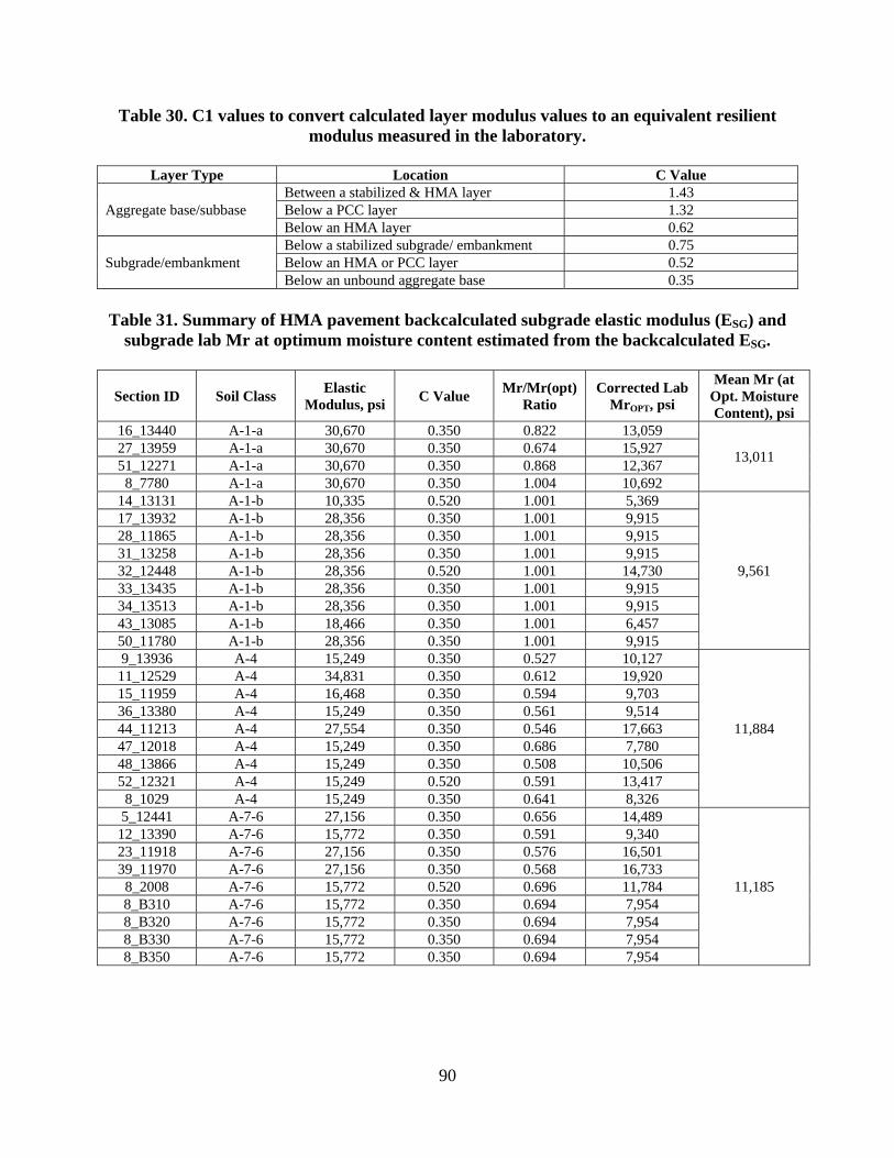
90

Table 30. C1 values to convert calculated layer modulus values to an equivalent resilient modulus measured in the laboratory.

Layer Type Location C Value

Aggregate base/subbase Between a stabilized & HMA layer 1.43 Below a PCC layer 1.32 Below an HMA layer 0.62

Subgrade/embankment Below a stabilized subgrade/ embankment 0.75 Below an HMA or PCC layer 0.52 Below an unbound aggregate base 0.35

Table 31. Summary of HMA pavement backcalculated subgrade elastic modulus (ESG) and

subgrade lab Mr at optimum moisture content estimated from the backcalculated ESG.

Section ID Soil Class Elastic

Modulus, psi C Value

Mr/Mr(opt) Ratio

Corrected Lab MrOPT, psi

Mean Mr (at Opt. Moisture Content), psi

16_13440 A-1-a 30,670 0.350 0.822 13,059

13,011 27_13959 A-1-a 30,670 0.350 0.674 15,927 51_12271 A-1-a 30,670 0.350 0.868 12,367 8_7780 A-1-a 30,670 0.350 1.004 10,692

14_13131 A-1-b 10,335 0.520 1.001 5,369

9,561

17_13932 A-1-b 28,356 0.350 1.001 9,915 28_11865 A-1-b 28,356 0.350 1.001 9,915 31_13258 A-1-b 28,356 0.350 1.001 9,915 32_12448 A-1-b 28,356 0.520 1.001 14,730 33_13435 A-1-b 28,356 0.350 1.001 9,915 34_13513 A-1-b 28,356 0.350 1.001 9,915 43_13085 A-1-b 18,466 0.350 1.001 6,457 50_11780 A-1-b 28,356 0.350 1.001 9,915 9_13936 A-4 15,249 0.350 0.527 10,127

11,884

11_12529 A-4 34,831 0.350 0.612 19,920 15_11959 A-4 16,468 0.350 0.594 9,703 36_13380 A-4 15,249 0.350 0.561 9,514 44_11213 A-4 27,554 0.350 0.546 17,663 47_12018 A-4 15,249 0.350 0.686 7,780 48_13866 A-4 15,249 0.350 0.508 10,506 52_12321 A-4 15,249 0.520 0.591 13,417 8_1029 A-4 15,249 0.350 0.641 8,326 5_12441 A-7-6 27,156 0.350 0.656 14,489

11,185

12_13390 A-7-6 15,772 0.350 0.591 9,340 23_11918 A-7-6 27,156 0.350 0.576 16,501 39_11970 A-7-6 27,156 0.350 0.568 16,733 8_2008 A-7-6 15,772 0.520 0.696 11,784 8_B310 A-7-6 15,772 0.350 0.694 7,954 8_B320 A-7-6 15,772 0.350 0.694 7,954 8_B330 A-7-6 15,772 0.350 0.694 7,954 8_B350 A-7-6 15,772 0.350 0.694 7,954

91

Table 31. Summary of backcalculated subgrade elastic modulus (ESG) and subgrade lab Mr at optimum moisture content estimated from the backcalculated ESG, continued.

Section ID Soil Class Elastic

Modulus, psi C Value

Mr/Mr(opt) Ratio

Corrected Lab MrOPT,

psi


35_13087 A-2 27,461 0.350 1.001 9,602

8,732

4_91044 A-2-4 22,460 0.520 1.001 11,668 7_13817 A-2-4 22,460 0.350 1.001 7,853

42_12153 A-2-4 19,198 0.350 1.002 6,706 49_13864 A-2-4 22,460 0.350 1.001 7,853 8_6013 A-2-4 24,443 0.350 1.001 8,547

37_92976 A-2-5 25,439 0.350 1.001 8,895 8_12685 A-6 16,020 0.350 0.582 9,634

15,932

10_12393 A-6 21,921 0.350 0.642 11,951 21_91094 A-6 26,858 0.520 0.646 21,619 22_12297 A-6 22,128 0.350 0.561 13,805 38_13505 A-6 16,020 0.350 0.589 9,520 41_13325 A-6 16,020 0.350 0.734 7,639 45_13106 A-6 16,020 0.350 0.628 8,928 8_0501 A-6 23,014 0.520 0.628 19,056 8_0502 A-6 29,762 0.520 0.627 24,683 8_0503 A-6 32,029 0.520 0.627 26,563 8_0504 A-6 27,983 0.520 0.627 23,208 8_0505 A-6 22,614 0.520 0.628 18,725 8_0506 A-6 23,249 0.520 0.628 19,251 8_0507 A-6 23,083 0.520 0.627 19,144 8_0508 A-6 25,123 0.520 0.627 20,836 8_0509 A-6 34,171 0.520 0.628 28,294 8_0559 A-6 29,635 0.520 0.626 24,617 8_0560 A-6 24,780 0.520 0.627 20,551 8_1047 A-6 22,185 0.350 0.678 11,452 8_1053 A-6 23,181 0.350 0.641 12,657 8_1057 A-6 15,769 0.350 0.674 8,189 8_6002 A-6 16,020 0.350 0.641 8,747 8_7781 A-6 19,843 0.350 0.671 10,350 8_7783 A-6 36,028 0.350 0.646 19,520 8_A310 A-6 23,181 0.350 0.643 12,618 8_A320 A-6 23,181 0.350 0.643 12,618 8_A330 A-6 23,181 0.350 0.643 12,618 8_A340 A-6 23,181 0.350 0.643 12,618 8_A350 A-6 23,181 0.350 0.643 12,618

For new JPCP projects, equivalent subgrade Mr (at optimum moisture) was estimated iteratively using the MEPDG as follows:

1. Obtain backcalculated modulus of subgrade reaction (k-value) at in situ moisture content through backcalculation.

2. Run MEPDG using default subgrade Mr for given soil class. Obtain monthly in situ (predicted) k-value for the subgrade layer and MEPDG estimated in situ moisture.

3. Compare MEPDG estimates of k-value and in situ moisture with backcalculated k-value and field-measured in situ moisture content values.

92

4. If there are significant differences between the two k-values (> 10 percent), adjust the default subgrade Mr for the given soil class and repeat steps 2 and 3 until the difference is less than 10 percent and obtain default subgrade Mr for the given project.

Table 32 presents a summary of backcalculated subgrade k-value and subgrade lab Mr at optimum moisture content estimated from the backcalculated subgrade k-value, along with subgrade soil AASHTO classification. Table 32. Summary of rigid pavement backcalculated subgrade k-value and subgrade lab

Mr at optimum moisture content estimated from the backcalculated subgrade k-value.

Section ID AASHTO Soil Class

Backcalculated Dynamic k-Value, psi/in

Backcalculated Elastic Modulus, in


18-12187 A-1-a 376 18,000

14,900 54-11546 A-1-a 240 15,500 55-93015 A-1-a 170 10,000 8_3032 A-1-a 250 13,000

13-10175 A-1-b 270 18,000 19-92021 A-2-4 260 16,500

13,808

8_0213 A-2-4 190 12,000 8_0215 A-2-4 286 22,000 8_0216 A-2-4 190 12,500 8_0218 A-2-4 154 8,000 8_0219 A-2-4 170 9,000 8_0220 A-2-4 195 10,500 8_0222 A-2-4 198 13,000 8_0223 A-2-4 165 10,000 8_0259 A-2-4 228 16,500 8_9019 A-2-4 271 16,500 8_0214 A-2-6 218 16,000 8_7776 A-2-6 240 17,000

29-89168 A-3 180 8,000 8,000 26-93216 A-4 206 18,000

18,200 46-00000 A-4 216 15,000 2-11327 A-4 400 24,000 3-88452 A-4 334 20,000 8_9020 A-4 260 14,000 6-91022 A-6 124 6,300

12,860 8_0217 A-6 160 9,000 8_0221 A-6 212 17,000 8_0224 A-6 181 11,000 1-11328 A-6 444 21,000

25-10326 A-7-6 190 13,000 12,000

53-84076 A-7-6 165 11,000 On average, multiplying ESG by a factor of 0.39 for coarse-grained soils and 0.64 for fine-grained subgrade soils provides an approximate value for subgrade resilient modulus Mr at optimum moisture content. For PCC pavements, MEPDG input subgrade resilient modulus Mr at optimum moisture can be obtained by using the relationship below (also see Figure 57):

Mr(opt)= 60.754*k-value (4)

93

Figure 57. Plots showing relationship between backcalculated k-value and MEPDG input

subgrade resilient modulus Mr at optimum moisture for month of FWD testing.

Laboratory Testing Laboratory-prepared HMA and PCC specimens were tested and characterized using CDOT, AASHTO, and ASTM test protocols as well as nonstandardized test methods to obtain properties required for computing default CDOT MEPDG material inputs. In total, several replicates of nine typical CDOT HMA mixtures were develop along with standard CDOT PCC mixtures with different coarse aggregate types. The following laboratory tests were conducted:

HMA. o Dynamic modulus test. o Indirect tensile strength and creep compliance test. o Repeated load deformation test. o Rut testing using the Hamburg Wheel Tracking (HWT) test.

PCC. o Fresh concrete and mix properties (e.g., slump). o Compressive strength. o Flexural strength. o CTE. o Elastic modulus.

y = 60.754xR² = 0.6876

5,000

10,000

15,000

20,000

25,000

30,000

100 150 200 250 300 350 400 450 500

MEPDG Input Mr (opt)

Backcalculated Subgrade k‐value. psi/in

94

The following sections present a detailed description of the laboratory testing and outcomes (default MEPDG materials inputs). HMA Mixtures Characterization Description of HMA Mixtures Laboratory testing was conducted on nine HMA samples and field cores—four conventional HMA, three HMA with PMA, and two SMA. The goal was to determine default HMA inputs such as dynamic modulus, creep compliance, indirect tensile strength, and in-place air voids and volumetric binder content. Tables 33 and 34 describe the nine CDOT mixes.

Table 33. CDOT mixes tested in the laboratory to develop MEPDG default inputs.

Mix ID Sample No. Mix Type Binder Grade Mix ID Gradation

FS1918-9 United 58-28-2 Conv HMA PG 58-28 FS1918-9 SX FS1919-2 #181603 SMA PG 76-28 FS1919-2 SMA FS1920-3 #183476 Conv HMA PG 58-28 FS1920-3 SX FS1938-1 #16967C Conv HMA PG 64-22 FS1938-1 SX FS1939-5 #194140 PMA PG 76-28 FS1939-5 SX FS1940-5 #17144B Conv HMA PG 58-28 FS1940-5 SX FS1958-5 Wolf Creek Pass PMA PG 58-34 FS1958-5 SX

FS1959-8 I70 Gypsum to

Eagle PMA PG 64-28 FS1959-8 SX

FS1960-2 I25 N of SH34 SMA PG 76-28 FS1960-2 SMA

Table 34. Volumetric properties and gradation of the selected typical CDOT HMA mixes.

ID & Properties Mix ID

FS1918-9 FS1920-3 FS1938-1 FS1940-5

Sample no. United 58-28-2 #183476 #16967C #17144B

Binder grade PG 58-28 PG 58-28 PG 64-22 PG 58-28

Gradation SX SX SX SX

Passing ¾” sieve 100 100 100 100

Passing ⅜” sieve 83 88 89 82

Passing No 4 sieve 53 62 69 56

Passing No. 200 sieve 6.5 7.1 6.8 5.9

Mix AC binder 5 5.6 5.4 5.5

Voids in mineral aggregate (VMA) (%)

16.2 17 16.3 17.2

Voids filled with asphalt (VFA) (%)

65.9 64.1 68.5 68.2

Air voids (%) 5.5 6.1 5.1 5.5

Effective volumetric moisture content (Vbeff) (%)

10.7 10.9 11.2 11.7

95

Table 34. Volumetric properties and gradation of the 9 selected typical CDOT HMA mixes, continued.

ID & Properties Mix ID

FS1958-5 FS1959-8 FS1919-2 FS1939-5 FS1960-2

Sample no. Wolf Creek

Pass I70 Gypsum to

Eagle #181603 #194140 I25 N of SH34

Binder grade PG 58-34 PG 64-28 PG 76-28 PG 76-28 PG 76-28

Gradation SX SX SMA SX SMA

Passing ¾” sieve 100 95 95 100 100

Passing ⅜” sieve 81 87 46 87 69

Passing No 4 sieve 54 65 22 62 25

Passing No. 200 sieve 5 7.1 8 6.6 8.1

Mix AC binder 7 5.4 6.2 5.4 6.5

VMA (%) 19.6 16.4 16.9 16.3 17.1

VFA (%) 73.4 65.5 72 68.2 76.8

Air voids (%) 5.2 5.7 4.7 5.2 4.0

Vbeff (%) 14.4 10.7 12.2 11.1 13.1

HMA Dynamic Modulus Testing The dynamic modulus values were measured in accordance with AASHTO TP 62, Standard Method of Test for Determining Dynamic Modulus of Hot Mix Asphalt (HMA), for a combination of five test temperatures and five test frequencies, as required for MEPDG Level 1. The results are presented in Table 35.

Table 35. Dynamic modulus values of typical CDOT HMA mixtures.

Mix ID Temperature

(°F) Testing Frequency

25 Hz 10 Hz 1 Hz 0.5 Hz

FS1918 (PG 58-28,

Gradation SX)

14 2,900,099 2,818,038 2,537,265 2,428,970 40 2,257,965 2,075,896 1,549,873 1,381,660 70 1,112,586 906,142 484,540 390,933 100 323,971 239,391 111,912 90,140 130 86,719 66,421 37,785 32,918

FS1919 (PG 76-28,

Gradation SMA)

14 2,758,515 2,662,007 2,351,059 2,237,401 40 2,045,581 1,865,812 1,378,519 1,230,679 70 980,835 809,521 464,947 387,592 100 323,623 252,537 137,906 116,443 130 110,901 90,227 58,256 52,283

FS1920 (PG 58-28,

Gradation SX)

14 2,788,941 2,698,644 2,397,288 2,283,742 40 2,100,335 1,914,978 1,397,712 1,237,621 70 978,820 791,037 418,926 338,214 100 277,921 206,455 98,884 80,365 130 76,798 59,571 34,858 30,574

96

Table 35. Dynamic modulus values of typical CDOT HMA mixtures.

Mix ID Temperature

(°F) Testing Frequency

25 Hz 10 Hz 1 Hz 0.5 Hz

FS1938 (PG 64-22,

Gradation SX)

14 2,950,163 2,887,740 2,680,448 2,601,704 40 2,417,122 2,276,774 1,860,432 1,720,558 70 1,391,643 1,198,776 753,641 639,073 100 496,933 385,970 194,405 157,140 130 135,576 102,799 53,830 45,192

FS1939 (PG 76-28,

Gradation SX)

14 2,776,809 2,674,640 2,339,581 2,215,718 40 2,037,766 1,843,321 1,317,308 1,159,645 70 930,020 750,969 404,138 330,013 100 281,928 214,540 111,276 92,946 130 91,132 73,216 46,546 41,736

FS1940 (PG 58-28,

Gradation SX)

14 2,849,460 2,764,473 2,473,915 2,362,175 40 2,156,745 1,967,527 1,433,170 1,266,797 70 971,195 779,370 407,026 328,213 100 260,831 194,792 97,113 80,429 130 75,318 60,298 38,496 34,650

FS1958 (PG 58-34,

Gradation SX)

14 2,436,678 2,299,130 1,871,731 1,723,419 40 1,567,260 1,358,215 854,152 721,055 70 575,990 443,437 217,831 175,189 100 157,715 119,392 63,837 54,320 130 55,485 45,673 31,101 28,460

FS1959 (PG 64-28,

Gradation SX)

14 2,645,996 2,535,875 2,190,535 2,067,626 40 1,867,004 1,680,477 1,194,431 1,052,657 70 822,141 666,566 366,356 301,596 100 249,892 192,068 101,355 84,788 130 80,788 64,960 40,838 36,386

FS1960 (PG 76-28,

Gradation SMA)

14 2,773,716 2,674,443 2,352,150 2,233,847 40 2,077,688 1,893,732 1,393,018 1,241,085 70 1,031,593 852,589 491,260 410,107 100 362,392 283,780 156,557 132,697 130 132,036 107,672 70,033 63,020

The dynamic moduli of the laboratory-tested HMA mixes were evaluated to determine reasonableness and how they compared with MEPDG Level 3 “global” defaults. To check for reasonableness, the researchers evaluted trends in the measured HMA dynamic modulus with increasing test temperature and increasing loading frequency. As expected, HMA dynamic modulus increased with increasing loading frequency and decreased with increased test temperature. Next was to compare the test and Level 3 global dynamic modulus estimates. This was done by fitting the CDOT test data to the MEPDG dynamic modulus master curve (by developing master curve parameters for each mix type) and comparing trends in the CDOT laboratory-determined and MEPDG master curves for each mix type. The HMA dynamic modulus master curve equation is presented below: (5)

r

a

TT

Ef

e

E11

14714.19log

1

*log

97

where = log (Emin) = log (Emax) - log (Emin) f = frequency, Hz T = temperature of interest, ˚K Tr = reference temperature, ˚K Ea = activation parameter = shape parameters

The fitted master curve parameters are presented in Table 36. Comparisons of HMA dynamic modulus E* for different binder grades, mix types (Superpave vs. SMA), and hierarchal level of estimation (Level 1 vs. Level 3) are presented in Figures 58 through 63.

Table 36. HMA dynamic modulus master curve parameters for typical CDOT HMA mixtures.

Mix ID Ea

FS1918-9 4.110062 2.403987 -0.6423 -0.5568 205347.9 FS1919-2 4.366954 2.146171 -0.4303 -0.5050 209368.3 FS1920-3 4.087468 2.419617 -0.5505 -0.5393 206824.9 FS1938-1 3.952260 2.562730 -1.1046 -0.4794 223377.0 FS1939-5 4.297267 2.217203 -0.3660 -0.5384 202863.5 FS1940-5 4.250315 2.258170 -0.4136 -0.5653 211738.7 FS1958-5 4.211077 2.284814 0.0269 -0.5522 194062.3 FS1959-8 4.174802 2.337297 -0.3819 -0.4919 208726.3 FS1960-2 4.470080 2.044498 -0.3943 -0.5227 199965.8

Figure 58. Comparison of HMA dynamic modulus E* for different binder grades.

0

500000

1000000

1500000

2000000

2500000

3000000

3500000

0.00001 0.001 0.1 10 1000 100000 10000000

Dynamic M

odulus, psi

Reduced Frequency, Hz

PG 58‐28 SX

PG64‐22 SX

PG 76‐28 SX

98

Figure 59. Comparison of HMA dynamic modulus E* for Superpave and SMA mixes.

Figure 60. Comparison of HMA dynamic modulus E* for Level 1 and Level 3 estimates (Mix FS-1938 (PG 64-22 & SX)).

0

500000

1000000

1500000

2000000

2500000

3000000

0.00001 0.001 0.1 10 1000 100000 10000000

Dynamic M

odulus, psi


PG 76‐28 SX

PG 76‐28 SMA

0

500000

1000000

1500000

2000000

2500000

3000000

3500000

4000000

4500000

5000000

0.00001 0.001 0.1 10 1000 100000 10000000

Dynamic M

odulus, psi


DARWin‐ME Defaults

Lab Measured

99



0

500000

1000000

1500000

2000000

2500000

3000000

3500000

4000000

0.00001 0.001 0.1 10 1000 100000 10000000

Dynamic M

odulus, psi



Lab Measured

0

500000

1000000

1500000

2000000

2500000

3000000

3500000

4000000

0.00001 0.001 0.1 10 1000 100000 10000000

Dynamic M

odulus, psi



Lab Measured

100

Figure 63. Comparison of HMA dynamic modulus E* for Level 1 and Level 3 estimates (Mix FS-1919 (PG 76-28 & SMA)).

The following were observed from the comparisons:

Binder type had a significant impact on E* for loading frequencies ranging from 0.1 to 10,000 Hz.

Superpave and SMA mixes produced similar estimates of E* for the frequency range tested.

The MEPDG global E* model significantly overestimated E* for higher test frequencies (> 1000 Hz) for SMA and PMA mixes.

Thus, it was recommended that the CDOT HMA dynamic modulus values presented in Table 35 be adopted for use as default statewide (Level 2/3) inputs in lieu of actual project-specific dynamic test values (Level 1). HMA Creep Compliance and Indirect Tensile Strength HMA creep compliance—D(t)—is the ratio of time-dependent strain response to a constant stress input at controlled temperature/loading, and it is a required input for the MEPDG HMA transverse “thermal” cracking model (TCMODEL). Laboratory testing for D(t) was done using AASHTO TP 322, Standard Method of Test for Determining the Creep Compliance and Strength of Hot-Mix Asphalt (HMA) Using the Indirect Tensile Test Device. Testing was done for all nine selected CDOT mixes at three low test temperatures (-4 oF, 14 oF, and 32 oF) and 7 loading times (1 sec, 2 sec, 5 sec, 10 sec, 20 sec, 50 sec, and 100 sec). The test results are presented in Table 37. HMA indirect tensile strength (IDT)—the strength of the HMA sample when subjected to indirect tension (by applying compressive load diametrically)—is also a key input required by the MEPDG TCMODEL. IDT testing was done according to AASHTO TP 322. The reference test temperature was 14 °F. The test results are presented in Table 38.

0

500000

1000000

1500000

2000000

2500000

3000000

3500000

0.00001 0.001 0.1 10 1000 100000 10000000

Dynamic M

odulus, psi



Lab Measured

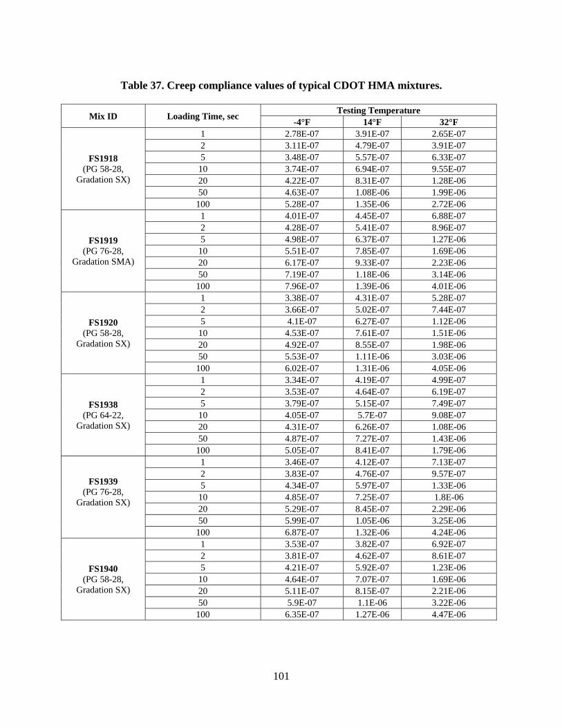
101

Table 37. Creep compliance values of typical CDOT HMA mixtures.

Mix ID Loading Time, sec Testing Temperature

-4°F 14°F 32°F

FS1918 (PG 58-28,

Gradation SX)

1 2.78E-07 3.91E-07 2.65E-07 2 3.11E-07 4.79E-07 3.91E-07 5 3.48E-07 5.57E-07 6.33E-07

10 3.74E-07 6.94E-07 9.55E-07 20 4.22E-07 8.31E-07 1.28E-06 50 4.63E-07 1.08E-06 1.99E-06

100 5.28E-07 1.35E-06 2.72E-06

FS1919 (PG 76-28,

Gradation SMA)

1 4.01E-07 4.45E-07 6.88E-07 2 4.28E-07 5.41E-07 8.96E-07 5 4.98E-07 6.37E-07 1.27E-06

10 5.51E-07 7.85E-07 1.69E-06 20 6.17E-07 9.33E-07 2.23E-06 50 7.19E-07 1.18E-06 3.14E-06

100 7.96E-07 1.39E-06 4.01E-06

FS1920 (PG 58-28,

Gradation SX)

1 3.38E-07 4.31E-07 5.28E-07 2 3.66E-07 5.02E-07 7.44E-07 5 4.1E-07 6.27E-07 1.12E-06

10 4.53E-07 7.61E-07 1.51E-06 20 4.92E-07 8.55E-07 1.98E-06 50 5.53E-07 1.11E-06 3.03E-06

100 6.02E-07 1.31E-06 4.05E-06

FS1938 (PG 64-22,

Gradation SX)

1 3.34E-07 4.19E-07 4.99E-07 2 3.53E-07 4.64E-07 6.19E-07 5 3.79E-07 5.15E-07 7.49E-07

10 4.05E-07 5.7E-07 9.08E-07 20 4.31E-07 6.26E-07 1.08E-06 50 4.87E-07 7.27E-07 1.43E-06

100 5.05E-07 8.41E-07 1.79E-06

FS1939 (PG 76-28,

Gradation SX)

1 3.46E-07 4.12E-07 7.13E-07 2 3.83E-07 4.76E-07 9.57E-07 5 4.34E-07 5.97E-07 1.33E-06

10 4.85E-07 7.25E-07 1.8E-06 20 5.29E-07 8.45E-07 2.29E-06 50 5.99E-07 1.05E-06 3.25E-06

100 6.87E-07 1.32E-06 4.24E-06

FS1940 (PG 58-28,

Gradation SX)

1 3.53E-07 3.82E-07 6.92E-07 2 3.81E-07 4.62E-07 8.61E-07 5 4.21E-07 5.92E-07 1.23E-06

10 4.64E-07 7.07E-07 1.69E-06 20 5.11E-07 8.15E-07 2.21E-06 50 5.9E-07 1.1E-06 3.22E-06

100 6.35E-07 1.27E-06 4.47E-06

102

Table 37. Creep compliance values of typical CDOT HMA mixtures, continued.

Mix ID Loading Time, sec Testing Temperature

-4°F 14°F 32°F

FS1958 (PG 58-34,

Gradation SX)

1 4.82E-07 5.95E-07 9.61E-07 2 5.30E-07 8.18E-07 1.48E-06 5 6.05E-07 1.05E-06 2.18E-06

10 6.85E-07 1.35E-06 3.14E-06 20 7.71E-07 1.62E-06 4.19E-06 50 8.72E-07 2.12E-06 6.23E-06

100 1.00E-06 2.63E-06 8.74E-06

FS1959 (PG 64-28,

Gradation SX)

1 3.61E-07 4.73E-07 7.12E-07 2 4.04E-07 5.74E-07 9.97E-07 5 4.51E-07 7.35E-07 1.52E-06

10 5.11E-07 8.78E-07 1.99E-06 20 5.67E-07 1.04E-06 2.59E-06 50 6.57E-07 1.37E-06 3.75E-06

100 7.68E-07 1.66E-06 4.66E-06

FS1960 (PG 76-28,

Gradation SMA)

1 3.64E-07 4.64E-07 7.35E-07 2 4.05E-07 5.70E-07 1.04E-06 5 4.43E-07 7.15E-07 1.51E-06

10 5.06E-07 8.79E-07 2.04E-06 20 5.48E-07 1.03E-06 2.61E-06 50 6.40E-07 1.31E-06 3.61E-06

100 7.44E-07 1.70E-06 4.69E-06

Table 38. Indirect tensile strength values of typical CDOT HMA mixtures.

Mix ID Indirect Tensile Strength at 14˚F

FS1918 (PG 58-28, Gradation SX) 555.9 FS1919 (PG 76-28, Gradation SMA) 515.0 FS1920 (PG 58-28, Gradation SX) 519.0 FS1938 (PG 64-22, Gradation SX) 451.0 FS1939 (PG 76-28, Gradation SX) 595.0 FS1940 (PG 58-28, Gradation SX) 451.0 FS1958 (PG 58-34, Gradation SX) 446.0 FS1959 (PG 64-28, Gradation SX) 519.0

FS1960 (PG 76-28, Gradation SMA) 566.0 Plots of creep compliance versus loading time were generated and evaluated to assess the reasonableness of the laboratory test values (see Figure 64). The observed trends (increasing creep compliance with increase time) were deemed reasonable. The Level 1 laboratory-measured and Level 3 MEPDG “global” model estimates of creep compliance and indirect tensile strength were compared statistically to determine whether the two sets of estimates were significantly different. A summary of the results is presented in Tables 39 and 40.

103

Figure 64. Laboratory-measured creep compliance versus loading time.

Table 39. Statistical comparison of Level 1 laboratory-tested and Level 3 MEPDG computed creep compliance for the selected CDOT HMA mixtures.

Mix ID Mix Type Binder Grade

Student t-testt-critical

at 95% CI Result

FS1918-9 Conv HMA PG 58-28 3.166 2.086 Significant FS1919-2 SMA PG 76-28 0.140 2.086 Not Significant FS1920-3 Conv HMA PG 58-28 6.006 2.086 Significant FS1938-1 Conv HMA PG 64-22 0.730 2.086 Not Significant FS1939-5 PMA PG 76-28 14.08 2.086 Significant FS1940-5 Conv HMA PG 58-28 0.183 2.086 Not Significant FS1958-5 PMA PG 58-34 0.941 2.086 Not Significant FS1959-8 PMA PG 64-28 2.719 2.086 Significant FS1960-2 SMA PG 76-28 1.281 2.086 Not Significant

1.0E‐07

1.0E‐06

1.0E‐05

1.0E‐04

1.0E‐03

1.0E+00 1.0E+02 1.0E+04 1.0E+06 1.0E+08

Creep

Complian

ce, 1/psi

Reduced Time, s (at ref temp ‐4 ˚F)

PG 64‐22 SX

PG 76‐28 SX

PG 58‐28 SX

PG 76‐28 SMA

104

Table 40. Statistical comparison of Level 1 laboratory-tested and Level 3 MEPDG computed indirect tensile strength for the selected CDOT HMA mixtures.

Mix ID Mix Type Binder Grade

Indirect Tensile Strength Result Level 1

Measured Level 3

Predicted FS1918-9 Conv HMA PG 58-28 555.9 420.3 Significant FS1919-2 SMA PG 76-28 515.0 453.2 Significant FS1920-3 Conv HMA PG 58-28 519.0 377.5 Significant FS1938-1 Conv HMA PG 64-22 451.0 376.3 Significant FS1939-5 PMA PG 76-28 595.0 431.3 Significant FS1940-5 Conv HMA PG 58-28 451.0 382.0 Significant FS1958-5 PMA PG 58-34 446.0 397.5 Significant FS1959-8 PMA PG 64-28 519.0 424.6 Significant FS1960-2 SMA PG 76-28 566.0 445.8 Significant

The statistical evaluation showed no consensus that Level 3 predictive equations provide statistically similar values to those of Level 1 measurements. Thus, the Level 1 creep compliance estimates were deemed more representative of CDOT HMA materials. For IDT, Level 3 predictive equations consistently underestimated IDT strength values. Thus, the Level 1 IDT estimates were deemed more representative of CDOT HMA materials. HMA Repeated Load Permanent Deformation Test & Hamburg Wheel Tracking Test The MEPDG rutting model uses three main parameters—k1, k2, and k3—to characterize the nature and rate of progression of rutting in the HMA layer. The MEPDG models only the “primary” and “secondary” portions of rutting, shown in Figure 65, using equation 6: (6) where

p = plastic strain r = resilient strain kz = depth confinement factor

k1 = intercept term k2 = exponent of T (i.e. temperature) k3 = exponent of N (i.e. load repetitions)

r1, r2

, r3 = local calibration factors T = layer temperature (˚F) N = number of load repetitions

33221

1

** **10** rr kkkrz

r

p NTk

Figur

For this pdetermin

R H

For both permanenA plot ofrelationshprogressiHMA mirutting,” From botrutting m

Pte

Pru

Dp

P F

ob D

re 65. Progr

project, laboned using the

Repeated loadHWT test.

tests, samplnt deformatif permanent hip betweenion in the HMix “primary rand then the

th the RLPDmodel k1, k2,

erform repeaemperatures.lot permaneutting for the

Determine theermanent strlot interceptit the non-linbtain non-lin

Determine mi

ression of Hrepeated

ratory estime following t

d permanent

les of HMA ion is observdeformation the two evaMA layer berutting,” folle stripping/d

D and HWT t, and k3 as fo

ated load pe. nt strain vere given HMAe slope (m) arain versus lot computed Inear equationear model pix-specific k

HMA ruttingd load perm

mates of the Hests:

t deformation

are repeatedved and measn versus numaluated. As segins with anlowed by a s

disintegration

tests, informfollows:

rmanent def

rsus load repA mix. and intercepoad repetitioIs versus teston Is = d*(T)parameters dk1, k2, and k3

105

g with repea

manent defor

HMA rutting

n (RLPD) te

dly loaded insured along

mber of loadihown in Fig

n initial, almslow rate of n of the HMA

mation was ob

formation tes

etitions and

pt (Is) for theons curve (set temperature)n to the comd and n (see F3 rutting mod

ated load aprmation tes

g model para

est (Von Qui

n a controlledwith the num

ing repetitiongure 66, rutti

most instantancreeping of A “tertiary r

btained to es

st/HWT test

define prim

e secondary ree Figure 67e.

mputed Is andFigure 68).del paramete

pplication obsting.

ameters k1, k

intus et al. 2

d environmember of loadns is then deing developmneous compathe HMA m

rutting.”

stimate MEP

for a range

mary, seconda

rutting porti7).

d test temper

ers:

btained from

k2, and k3 we

012).

ent while ding repetitioeveloped andment and action of the

mix “seconda

PDG HMA

of test

ary, and terti

on of the

rature data an

m

ere

ons. d the

e ary

iary

nd

Figur

Figure

o k1 = loo k2 = no k3 = m

re 66. Exam

67. Plot shop

og(d). n (exponent om (average m

mple plot of p

owing slope ortion of pl

of Is = d*(T)m for the rang

permanent obtained fr

(m) and intlot of perma

106

)n model). ge of test tem

deformatiorom HWT t

tercept (Is) canent strain

mperatures).

on vs. numbtesting.

computed fn vs. load rep

ber of loadin

from the secpetitions.

ng repetition

condary rut

ns

tting

107

Figure 68. Plot of intercept (Is) vs. repeated load permanent deformation test temperature.

For this project, RLPD tests were conducted on the selected CDOT HMA mixes for up to 10,000 repeated load cycles, 3 test temperatures (20, 35, and 50 ˚C), HMA confinement pressure of 10 psi, and applied deviator stress of 70 psi. Three replicates of each of the HMA mixtures were tested. The HWT test was conducted on the selected CDOT HMA mixes at a test temperature of 55 ˚C for up to 10,000 loading cycles. Results from the two tests are presented in Tables 41 and 42. A comparison of k1, k2, and k3 parameters from the RLPD and HWT tests showed no direct relationship. Table 41. Estimates of HMA rutting model k1, k2, and k3 parameters for the selected CDOT

HMA mixtures using the repeated load permanent deformation test procedure (Von Quintus et al. 2012).

Mix ID Binder Grade Gradation m-slope, k3 n-slope, k2 log(d), k1

FS1918-9 PG 58-28 SX 0.137 2.068 -2.58 FS1919-2 PG 76-28 SMA 0.179 2.395 -3.159 FS1920-3 PG 58-28 SX 0.164 0.525 -1.169 FS1938-1 PG 64-22 SX 0.17 2.758 -3.506 FS1939-5 PG 76-28 SX 0.136 2.79 -3.357 FS1940-5 PG 58-28 SX 0.178 1.25 -1.892 FS1958-5 PG 58-34 SX 0.15 1.132 -1.582 FS1959-8 PG 64-28 SX 0.132 1.647 -2.214 FS1960-2 PG 76-28 SMA 0.185 0.952 -1.818

Mean 0.16 1.72 -2.36

y = 0.0033x1.2755

R² = 0.9815

0.00

0.10

0.20

0.30

0.40

0.50

0.60

0 20 40 60

Intercept , Is

Test Temp ˚C

Test Temp vs Intercept

108

Table 42. Estimates of HMA rutting model k1, k2, and k3 parameters for the selected CDOT HMA mixtures using the HWT test procedure.

Mix ID Binder Grade Gradation Max Rut Depth mm Intercept Slope

FS1918-9 PG 58-28 SX 2.02 0.1197 0.294 FS1919-2 PG 76-28 SMA N.A. N.A. N.A. FS1920-3 PG 58-28 SX 2.06 0.1533 0.284 FS1938-1 PG 64-22 SX 1.98 0.1111 0.314 FS1939-5 PG 76-28 SX 2.65 0.1641 0.291 FS1940-5 PG 58-28 SX 3.36 0.1437 0.334 FS1958-5 PG 58-34 SX 3.85 0.0374 0.512 FS1959-8 PG 64-28 SX N.A. N.A. N.A. FS1960-2 PG 76-28 SMA 2.46 N.A. N.A.

PCC Mixtures Characterization Description of PCC Mixtures Four PCC mix types were prepared in the laboratory and tested. The PCC mixtures were prepared following CDOT guidance for PCC mixtures to be used as paving materials. Table 43 presents mix proportions and fresh concrete properties of the selected typical CDOT PCC mixtures (including slump, air content, and unit weight). The following test protocols were used in ensuring that the PCC mixes (constituent proportions and fresh concrete properties) were in accordance with CDOT guidelines:

PCC slump: ASTM C143, Standard Test Method for Slump of Portland Cement Concrete.

PCC air content: ASTM C231, Standard Test Method for Air Content of Freshly Mixed Concrete by the Pressure Method.

PCC unit weight: ASTM C138, Standard Test Method for Unit Weight, Yield, and Air Content (Gravimetric) of Concrete.

The sources of aggregate and cement materials used in developing the PCC mixtures in the laboratory are presented in Table 44. The sources were selected to be as representative of Colorado aggregates used for pavement construction as much as possible, as aggregate type and source significantly impact PCC thermal properties. Laboratory specimens (standard 4-in-diameter by 8-in-high cylinders) of the typical mixtures were prepared and tested as described in the following sections.

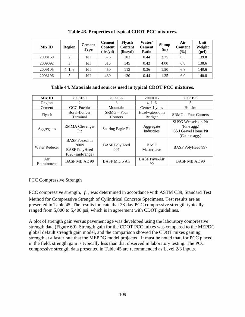
109

Table 43. Properties of typical CDOT PCC mixtures.

Mix ID Region Cement

Type

Cement Content (lbs/yd)

Flyash Content (lbs/yd)

Water/ Cement

Ratio

Slump (in)

Air Content

(%)

Unit Weight

(pcf) 2008160 2 I/II 575 102 0.44 3.75 6.3 139.8

2009092 3 I/II 515 145 0.42 4.00 6.8 138.6

2009105 4, 1, 6 I/II 450 113 0.36 1.50 6.8 140.6

2008196 5 I/II 480 120 0.44 1.25 6.0 140.8

Table 44. Materials and sources used in typical CDOT PCC mixtures.

Mix ID 2008160 2009092 2009105 2008196 Region 2 3 4, 1, 6 5 Cement GCC-Pueblo Mountain Cemex-Lyons Holsim

Flyash Boral-Denver

Terminal SRMG – Four

Corners Headwaters-Jim

Bridger SRMG – Four Corners

Aggregates RMMA Clevenger

Pit Soaring Eagle Pit

Aggregate Industries

SUSG Weaselskin Pit (Fine agg.)

C&J Gravel Home Pit (Coarse agg.)

Water Reducer

BASF Pozzolith 200N

BASF PolyHeed 1020 (mid-range)

BASF PolyHeed 997

BASF Masterpave

BASF PolyHeed 997

Air Entrainment

BASF MB AE 90 BASF Micro Air BASF Pave-Air

90 BASF MB AE 90

PCC Compressive Strength

PCC compressive strength, 'cf , was determined in accordance with ASTM C39, Standard Test

Method for Compressive Strength of Cylindrical Concrete Specimens. Test results are as presented in Table 45. The results indicate that 28-day PCC compressive strength typically ranged from 5,000 to 5,400 psi, which is in agreement with CDOT guidelines. A plot of strength gain versus pavement age was developed using the laboratory compressive strength data (Figure 69). Strength gain for the CDOT PCC mixes was compared to the MEPDG global default strength gain model, and the comparison showed the CDOT mixes gaining strength at a faster rate that the MEPDG model projected. It must be noted that, for PCC placed in the field, strength gain is typically less than that observed in laboratory testing. The PCC compressive strength data presented in Table 45 are recommended as Level 2/3 inputs.

110

Table 45. Compressive strength of typical CDOT PCC mixtures.

Mix Design ID

Region Compressive Strength, psi

7-day 14-day 28-day 90-day 365-day 2008160 2 4290 4720 5300 6590 6820 2009092 3 3740 4250 5020 5960 7140 2009105 4, 1, 6 3780 4330 5370 5560 6390 2008196 5 4110 4440 5340 5730 5990

Figure 69. Plot of compressive strength gain versus pavement age for CDOT PCC mixes.

PCC Flexural Strength PCC flexural strength MR was determined in accordance with ASTM C79, Standard Test Method for Flexural Strength of Concrete. The flexural strength test results are as presented in Table 46. The results indicate that 28-day PCC MR typically ranged from 700 to 900 psi, which is in agreement with CDOT guidelines. A plot of strength gain versus pavement age was developed using the laboratory-measured MR data (Figure 70). Strength gain for the CDOT PCC mixes was compared to the MEPDG global default strength gain model, and it showed the CDOT mixes initially gaining strength at a faster rate that the MEPDG predicted. At about 1 year, however, the rate of strength gain is similar. The PCC MR data presented in Table 46 are recommended as Level 2/3 inputs.

CDOTy = ‐0.0868x2 + 0.3424x + 0.9828

R² = 0.8759

0.6

0.7

0.8

0.9

1

1.1

1.2

1.3

1.4

1.5

‐0.8 ‐0.6 ‐0.4 ‐0.2 0 0.2 0.4 0.6 0.8 1 1.2 1.4

Strength Ratio (Given Age/28‐day)

Log (AGE/0.0767) (AGE in years)

CDOT MEPDG Log. (CDOT) Poly. (MEPDG)

111

Table 46. Flexural strength of typical CDOT PCC mixtures.

Mix Design ID

Region Flexural Strength, psi

7-day 14-day 28-day 90-day 365-day 2008160 2 660 760 900 935 940 2009092 3 570 645 730 810 850 2009105 4, 1, 6 560 620 710 730 735 2008196 5 640 705 905 965 970

Figure 70. Plot of flexural strength gain versus pavement age for CDOT PCC mixes.

The laboratory-tested PCC compressive strength ( '

cf ) and flexural strength (MR) data were used

to evaluate the reasonableness of the MEPDG “global” compressive strength and flexural strength relationship (see equation 7) by performing a paired t-test between the measured and MEPDG global equation-predicted MR. The paired t-test produced a p-value of 0.0006, which implied that there was a significant difference in the laboratory-measured and MEPDG “global” equation predicted MR at the 95 percent significant level. A review of the plot of laboratory-measured vs. MEPDG global equation-predicted MR indicated a good correlation between the two estimated of MR (R2 = 0.63) but with the MEPDG global equation underestimating MR for higher measured MR values.

5.0'5.9 cfMR (7)

Using the laboratory-measured 'cf and MR values, the project team performed further statistical

analysis to revise the MEPDG global MR equation parameter to remove the observed bias. The new CDOT statewide MR equation is presented as equation 8.

y = ‐0.1655x2 + 0.279x + 0.972R² = 0.9073

0

0.2

0.4

0.6

0.8

1

1.2

1.4

‐0.8 ‐0.6 ‐0.4 ‐0.2 0 0.2 0.4 0.6 0.8 1 1.2 1.4

Strength Ratio (Given Age/28‐day)

Log (AGE/0.0767)) (AGE in years)

CDOT MEPDG Poly. (CDOT) Poly. (MEPDG)

A paired value of percent sCDOT ststatewide

data. Not

Figu

PCC Elas PCC elasC469, StCompres28-day Eagreemen A plot ofdata (Figdefault stthe MEP

t-test betwe0.8613, whic

significant letatewide MRe equation is

te that this eq

ure 71. Plot

stic Modulu

stic modulusandard Test

ssion. The EP

EPCC typicallynt with CDO

f modulus gagure 72). Motrength gain DG predicte

een the measch implied th

evel. Figure 7R equation ans recommend

quation is va

of laboratoMEP

s and Poisso

s (EPCC) and Method for

PCC and PR ty ranged from

OT guideline

ain versus padulus gain fmodel, and

ed (for the pe

0MR

ured and CDhat there wa71 shows thend the MEPDded for estim

alid for 'cf r

ory-measurePDG global e

on’s Ratio

Poisson’s raStatic Modu

test results arm 3.5 to 4.3

es.

avement agefor the CDOTit showed th

eriod of 7 to

112

85.0'53.0 cf

DOT statewias no significe laboratory-DG global e

mating MR fr

ranging from

ed MR vs. Cequation-pr

atio (PR) werulus of Elastre as present million psi

was developT PCC mixehe CDOT mi

365 days).

de equation-cant differen-measured M

equation-predfrom measure

m 3,000 to 5,

CDOT statewredicted MR

re determineticity and Poted in Table and PR aver

ped using thes was compixes gaining

-predicted Mnce between MR plotted adicted MR. Ted compress

000 psi.

wide MR eqR.

ed in accordoisson’s Rati

47. The resuraged 0.2, w

he laboratorypared to the Mg strength at

(8

MR producedthe two at th

against the The new CDsive strength

quation and

ance with Aio of Concretults indicate

which is in

y-measured EMEPDG gloa faster rate

)

d a p-he 95

DOT h

d

ASTM te in

e that

EPCC obal

that

113

Table 47. Static elastic modulus and Poisson’s ratio of typical CDOT PCC mixtures.

Mix Design ID

Region Elastic Modulus, ksi Poisson’s

Ratio 7-day 14-day 28-day 90-day 365-day 2008160 2 3140 3260 3550 3970 4240 0.21 2009092 3 3560 3860 4300 4550 4980 0.2 2009105 4, 1, 6 3230 3500 4030 4240 4970 0.2 2008196 5 3280 3510 3930 4170 4210 0.21

Figure 72. Plot of elastic modulus gain versus pavement age for CDOT PCC mixes.

The laboratory-tested PCC 'cf and EPCC data were used to evaluate the reasonableness of the

MEPDG global 'cf and flexural strength relationship (see equation 9) by performing a paired t-

test between the measured and MEPDG global equation-predicted EPCC.

5.0'57000 cPCC fE (9)

The paired t-test produced a p-value of 0.0178, which implied that there was a significant difference between the laboratory-measured EPCC and MEPDG global equation-predicted EPCC at the 95 percent significant level. A review of the plot of laboratory-measured EPCC vs. MEPDG

y = ‐0.0501x2 + 0.2183x + 0.9818R² = 0.9173

0.6

0.7

0.8

0.9

1

1.1

1.2

1.3

‐0.8 ‐0.6 ‐0.4 ‐0.2 0 0.2 0.4 0.6 0.8 1 1.2 1.4

Modulus Ratio (Given Age/28‐day)

Log (AGE/0.0767) (AGE in years)

MEPDG CDOT Poly. (MEPDG) Poly. (CDOT)

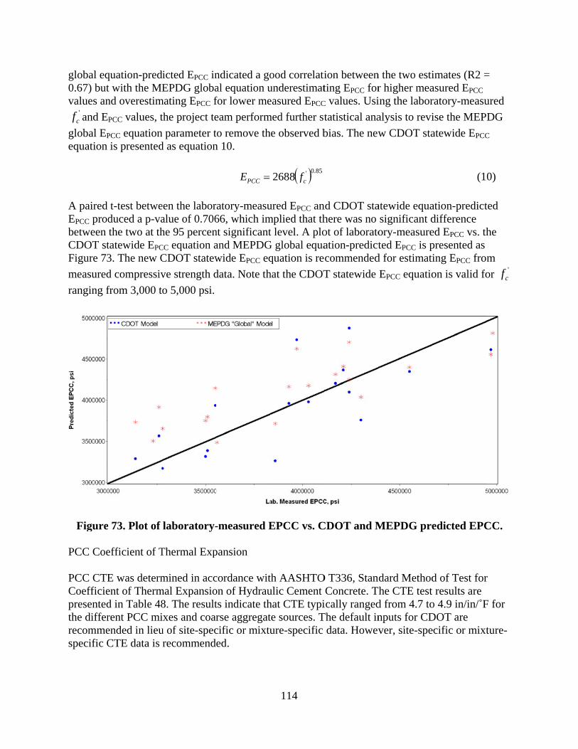
global eq0.67) butvalues an

'cf and E

global EP

equation

A paired EPCC prodbetween CDOT stFigure 73

measured

ranging f

Figure PCC Coe PCC CTECoefficiepresentedthe differrecommespecific C

quation-predt with the MEnd overestim

PCC values, t

PCC equationis presented

t-test betweduced a p-vathe two at thtatewide EPC

3. The new C

d compressiv

from 3,000 t

e 73. Plot of

efficient of T

E was determent of Thermd in Table 48rent PCC miended in lieuCTE data is

dicted EPCC inEPDG globa

mating EPCC f

the project te

n parameter td as equation

een the laboralue of 0.706he 95 percenCC equation aCDOT statew

ve strength d

o 5,000 psi.

laboratory-

Thermal Exp

mined in accmal Expansio8. The resultixes and coaru of site-specrecommend

ndicated a goal equation ufor lower me

eam perform

to remove thn 10.

PCCE

ratory-measu66, which imnt significantand MEPDGwide EPCC eq

data. Note th

-measured E

pansion

cordance witon of Hydrauts indicate thrse aggregatcific or mixtued.

114

ood correlatiunderestimateasured EPCC

med further st

he observed b

85.0'2688 cf

ured EPCC anmplied that tht level. A plo

G global equaquation is re

hat the CDOT

EPCC vs. C

th AASHTOulic Cement hat CTE typite sources. Ture-specific

ion betweenting EPCC for

C values. Usi

tatistical ana

bias. The new

nd CDOT stahere was no ot of laboratoation-predictcommended

T statewide

CDOT and M

O T336, StanConcrete. T

ically rangedThe default in

data. Howev

n the two estir higher meaing the labor

alysis to revi

w CDOT sta

atewide equasignificant dory-measureted EPCC is p

d for estimati

EPCC equatio

MEPDG pre

dard Methodhe CTE test

d from 4.7 tonputs for CDver, site-spe

imates (R2 =asured EPCC ratory-measu

ise the MEP

atewide EPCC

(1

ation-predictdifference ed EPCC vs. thpresented as ing EPCC fro

on is valid fo

edicted EPC

d of Test forresults are

o 4.9 in/in/˚FDOT are ecific or mixt

=

ured

DG

C

0)

ted

he

m

or 'cf

CC.

r

F for

ture-

115

Table 48. CTE values of typical CDOT PCC mixtures.

Mix ID Sample CTE in/in./˚C CTE in/in./˚F

2008160 1 8.5 4.72 2 8.5 4.72

2009092 1 8.8 4.89 2 8.6 4.78

2009105 1 8.8 4.89 2 8.7 4.83

2008196 1 8.8 4.89 2 8.6 4.78

Visual Distress Surveys Visual distress surveys were performed in accordance with the LTPP Distress Identification Manual to identify, measure, and record visual distresses (Miller & Bellinger, 2003). Other pertinent information collected included pavement details such as lane and slab width, joint spacing, ambient temperature during survey and FWD testing, and so on. Total rutting for flexible and composite (HMA-surfaced) pavements was measured using the straightedge method, while JPCP faulting was measured using the Georgia Digital Faultmeter. Figure 74 presents a sample of the distress survey maps used in recording identified distress present at the pavement surface. Once the survey was completed, the information on the distress maps and other paper records was transferred into an MS Access database that contained all key information regarding project location and type, survey date, surveyor name, section ID, and so on. Visual distress surveys were conducted only for the projects identified from the CDOT pavement management system, not the LTPP project sites. As possible, the cracking, rutting, faulting, and other data collected during the visual surveys were compared to the distress data available in the CDOT pavement management system database. This was only possible where the distress data were in a format compatible with LTPP and MEPDG. The comparisons were used to develop adjustment factors for correcting the CDOT pavement management system data to make them comparable to measured LTPP distress. This enabled the project team to include the CDOT pavement management system distress data in the project validation/calibration database, to the greatest extent possible.

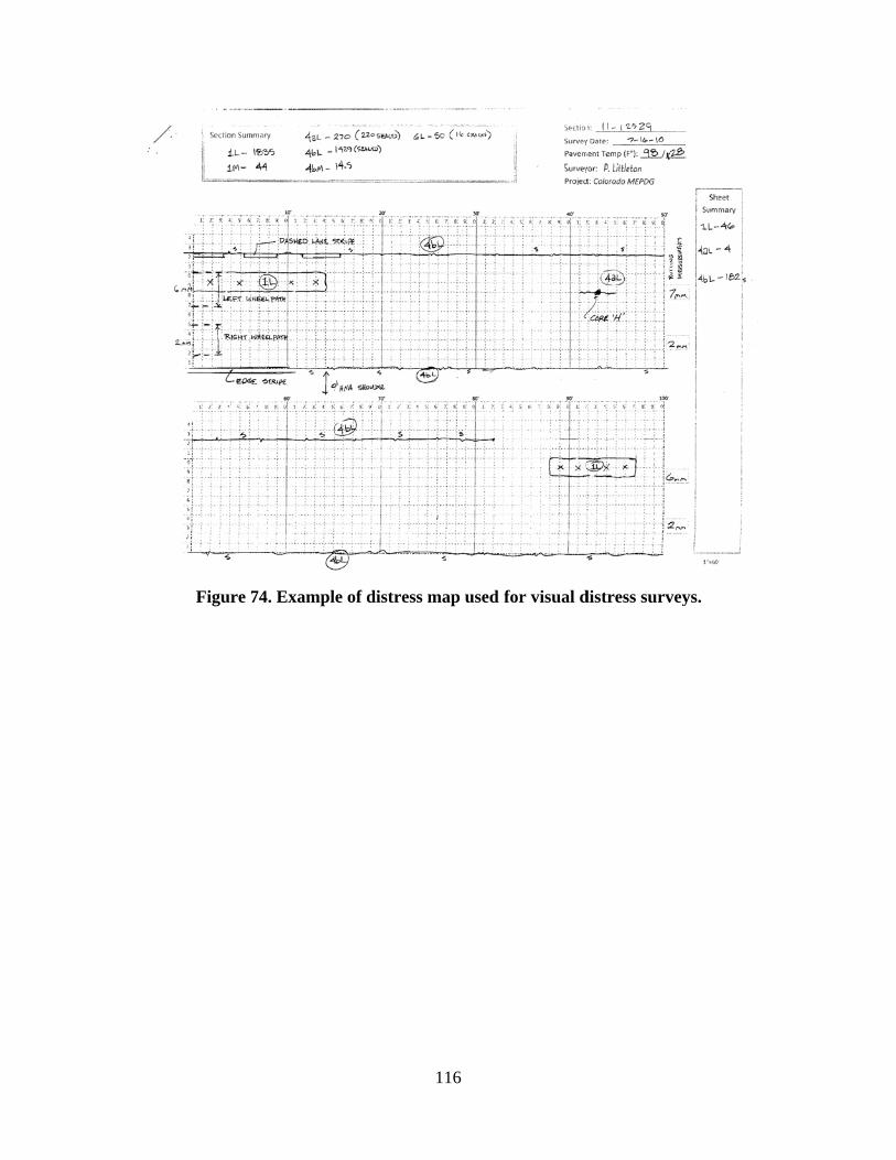
Figure 774. Example of distress

116

s map used for visual ddistress survveys.

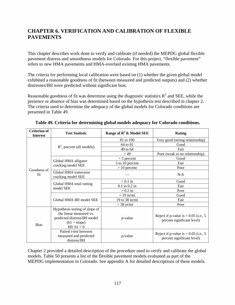
117

CHAPTER 6. VERIFICATION AND CALIBRATION OF FLEXIBLE PAVEMENTS This chapter describes work done to verify and calibrate (if needed) the MEPDG global flexible pavement distress and smoothness models for Colorado. For this project, “flexible pavement” refers to new HMA pavements and HMA-overlaid existing HMA pavements. The criteria for performing local calibration were based on (1) whether the given global model exhibited a reasonable goodness of fit (between measured and predicted outputs) and (2) whether distresses/IRI were predicted without significant bias. Reasonable goodness of fit was determine using the diagnostic statistics R2 and SEE, while the presence or absence of bias was determined based on the hypothesis test described in chapter 2. The criteria used to determine the adequacy of the global models for Colorado conditions are presented in Table 49.

Table 49. Criteria for determining global models adequacy for Colorado conditions.

Criterion of Interest

Test Statistic Range of R2 & Model SEE Rating

Goodness of fit

R2, percent (all models)

81 to 100 Very good (strong relationship) 64 to 81 Good 49 to 64 Fair

< 49 Poor (weak or no relationship)

Global HMA alligator cracking model SEE

< 5 percent Good 5 to 10 percent Fair > 10 percent Poor

Global HMA transverse cracking model SEE

— N/A

Global HMA total rutting model SEE

< 0.1 in Good 0.1 to 0.2 in Fair

> 0.2 in Poor

Global HMA IRI model SEE < 19 in/mi Good

19 to 38 in/mi Fair > 38 in/mi Poor

Bias

Hypothesis testing of slope of the linear measured vs.

predicted distress/IRI model (b1 = slope) H0: b1 = 0

p-value Reject if p-value is < 0.05 (i.e., 5

percent significant level)

Paired t-test between measured and predicted

distress/IRI p-value

Reject if p-value is < 0.05 (i.e., 5 percent significant level)

Chapter 2 provided a detailed description of the procedure used to verify and calibrate the global models. Table 50 presents a list of the flexible pavement models evaluated as part of the MEPDG implementation in Colorado. See appendix A for detailed descriptions of these models.

118

Table 50. MEPDG flexible pavement global models evaluated for Colorado local conditions.

Pavement Type

MEPDG Global Models Evaluated

HMA Alligator Cracking

HMA Transverse Cracking

Total Rutting

New HMA &

HMA/HMA IRI

HMA/HMA Reflected Alligator Cracking

New HMA HMA-overlaid existing HMA

Alligator Cracking Global MEDPG Alligator Cracking Model Verification Verification of the MEPDG global alligator cracking models for Colorado conditions consisted of the running the MEPDG with the global coefficients for all selected projects and evaluating goodness of fit and bias. Figure 75 shows a plot of cumulative fatigue damage versus alligator cracking for all Colorado HMA sections. Measured and MEPDG-predicted alligator cracking data were evaluated to determine model goodness of fit and bias in predicted alligator cracking. The results are presented in Table 51 and show the following:

Goodness of fit was generally poor, with an R2 < 40 percent, which implies a weak relationship between the MEPDG global model alligator cracking predictions and field-measured/observed cracking.

Both the paired t-test and predicted versus measured cracking slope p-value indicated the presence of bias in predicted alligator cracking (p-value < 0.05).

The plot presented in Figure 75 shows that the model consistently under-predicted alligator cracking with increasing levels of HMA fatigue damage, another indication of bias.

It was concluded that the MEPDG global alligator cracking model did not adequately predict alligator cracking for Colorado conditions. Local calibration of the MEPDG global alligator cracking model for Colorado was thus recommended.

FigureM

Table 5

R

Local Ca Descripti Local calHMA ancracking,

1. D2. A

norpr

3. AcaHcawn

4. Dm

e 75. VerificMEPDG glob

51. Results o

GoodR2, % 17.5

alibration of

ion of Local

libration of td HMA-ove, and reflecti

Determine theAdjust the M

eeded basedr eliminate brojects.

After determialibration co

HMA projectalibration co

while the locaeeded to imp

Details of spemodels coeffi

a. HMA

cation of thebal coefficien

of statisticalcracking

dness of Fit

0.175

the MEDPG

Calibration

the MEPDGerlaid existinion cracking

e cause of poEPDG HMA

d on informatbias. This ste

ining the locoefficient adjts) for only thoefficients foal calibrationprove overalecific HMA icients adjus

A fatigue mod

e HMA allignts, using C

l goodness og global mod

Statistica

SEE 5% lane area

G Alligator C

n Procedure

G alligator crang HMA pavg models. Ca

oor goodnesA fatigue andtion derived ep was done

cal calibratiojustments ushe reflection

or the fatiguen coefficientll goodness ofatigue crack

sted are presedel (allowab

119

gator crackColorado new

of fit and biadel for Colo

al Analysis

p-valua

Cracking Mo

acking modevement and thalibration con

ss of fit and bd alligator crfrom step 1using data f

on coefficiensing all projen cracking me cracking ants of the refleof fit and redking, alligatoented belowle number o

king and fatiw HMA pav

as evaluatioorado condit

Type

ue (paired t0.0059

odel for Colo

el was done the MEPDG nsisted of th

bias produceracking mod to improve from only th

nts in step 2, ects (new HM

model. In othnd alligator ection crackduce bias. or cracking,

w (see equatioof axle load a

igue damagvement proj

on of the MEtions.

Bias t-test) p

orado

simultaneouHMA fatigu

he following

ed by the glodel calibratio

goodness ofhe new HMA

perform a seMA and HMher words, thcracking mo

king model w

and reflections in Tableapplications,

ge models wijects only.

EPDG alliga

p-value (slop< 0.0001

usly for bothue, alligator steps:

obal models.on coefficienf fit and redu

A pavement

econd roundMA-overlaid he local odels were fiwere adjusted

ion cracking e 52). , N equation

ith

ator

pe)

h new

nts as uce

d of

ixed d as

n):

120

i. Global calibration coefficients (kf1, kf2, kf3). ii. Local calibration coefficients (βf1, βf2, βf3).

b. Alligator cracking model. i. Local/Global calibration coefficients (C1, C2, C3).

c. Reflected alligator cracking model. i. Global calibration coefficients (c, d).

5. Perform a final round of calibration coefficient adjustments, if needed, using all the local calibration estimates obtained in steps 2 through 4 as seed values. Adjustments to the calibration coefficients determined in steps 2 through 4 were constrained to ensure reasonableness of the final set of model coefficients.

A detailed description of the equations in Table 52 is presented in Appendix A.

Table 52. Description of HMA fatigue damage, HMA alligator cracking, and reflection “alligator” cracking models.

Model Type Model Description*

HMA fatigue damage 3322

11ffff k

HMAk

tfHfHMAf ECCkN

HMA alligator cracking

))((

4*22

*11160

1BottomDILogCCCCBottom

e

CFC

HMA reflection “alligator” cracking bdtaceRC

1

100

Summary of Alligator Cracking Model Local Calibration Results The researchers investigated the possible causes of poor goodness of fit and bias, and no obvious reasons were found (such as erroneous inputs). Thus, local calibration proceeded as previously described. Calibration of the MEPDG global models using CDOT input data was done using nonlinear model optimization tools available in the SAS statistical software. Adjusted HMA fatigue damage and alligator cracking global model coefficients are presented in Table 53 and shows that four of the nine global coefficients were adjusted. The goodness of fit and bias statistics are presented in Table 54 and show an adequate goodness of fit with minimal bias for the locally calibrated alligator cracking and fatigue damage models developed using new HMA projects only.

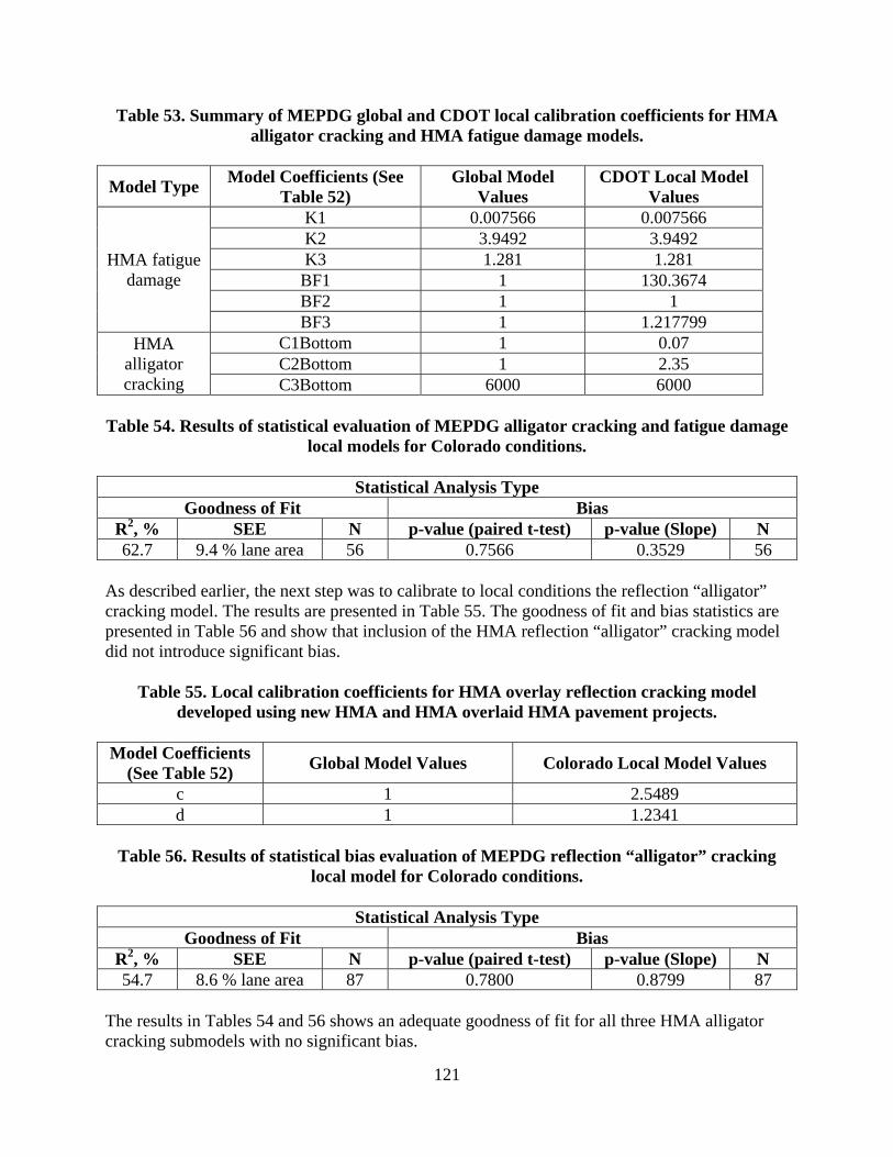
121

Table 53. Summary of MEPDG global and CDOT local calibration coefficients for HMA alligator cracking and HMA fatigue damage models.

Model Type Model Coefficients (See

Table 52) Global Model

ValuesCDOT Local Model

Values

HMA fatigue damage

K1 0.007566 0.007566 K2 3.9492 3.9492 K3 1.281 1.281

BF1 1 130.3674 BF2 1 1 BF3 1 1.217799

HMA alligator cracking

C1Bottom 1 0.07 C2Bottom 1 2.35 C3Bottom 6000 6000

Table 54. Results of statistical evaluation of MEPDG alligator cracking and fatigue damage

local models for Colorado conditions.

Statistical Analysis Type Goodness of Fit Bias

R2, % SEE N p-value (paired t-test) p-value (Slope) N 62.7 9.4 % lane area 56 0.7566 0.3529 56

As described earlier, the next step was to calibrate to local conditions the reflection “alligator” cracking model. The results are presented in Table 55. The goodness of fit and bias statistics are presented in Table 56 and show that inclusion of the HMA reflection “alligator” cracking model did not introduce significant bias.

Table 55. Local calibration coefficients for HMA overlay reflection cracking model developed using new HMA and HMA overlaid HMA pavement projects.

Model Coefficients

(See Table 52) Global Model Values Colorado Local Model Values

c 1 2.5489 d 1 1.2341

Table 56. Results of statistical bias evaluation of MEPDG reflection “alligator” cracking

local model for Colorado conditions.

Statistical Analysis Type Goodness of Fit Bias

R2, % SEE N p-value (paired t-test) p-value (Slope) N 54.7 8.6 % lane area 87 0.7800 0.8799 87

The results in Tables 54 and 56 shows an adequate goodness of fit for all three HMA alligator cracking submodels with no significant bias.

Figure 76alligator cracking 77. Figurnew HM Local calmodels paccuracyglobal m The new bias and HMA pa

Figu

dama

6 presents a cracking mowith HMA

res 78 througA pavement

libration of tproduced CDy and minimaodels to 52.5

models willwill producevement desi

ure 76. Plot ge develope

R2 = 62.7 pSEE = 9.4N = 56

plot of HMAodel predicteoverlay age gh 81 illustrat and HMA-o

the HMA fatDOT-specifical bias. Good5 percent, w

l increase thee for CDOT gns at the de

showing pred using ME

percent % lane area

A fatigue damed cracking. for different

ate the CDOoverlaid HM

tigue, alligatc models thadness of fit c

while SEE inc

e accuracy omore accura

esired design

edicted HMEPDG mode

pave

a

122

mage versusA plot showt HMA over

OT local modMA pavemen

tor cracking,at predict allicharacterizedcreased from

of alligator crate and optimn reliability.

MA alligatorels with CDements only)

s field-measuwing the progrlay thicknesdel predictionnt.

, and reflectiigator crackid using R2 in

m 5 to 17.1 p

racking predmum (lower

r cracking vOT local co).

ured and CDgression of rsses is presenn of alligato

ion “alligatoing distress wncreased fromercent lane a

dictions whilcost) new an

versus compoefficients (f

DOT local reflection nted in Figur

or cracking fo

or” cracking with adequatm 17.5 for tharea.

le minimizinnd overlaid

puted fatigufor new HM

re for

te he

ng

e MA

Figur

Figur

BU C

rack

ing, %

Ln A

rea

1

Alligator Cracking, % Lan

e Area

re 77. Plot s

re 78. Plot o

0102030405060708090

100

0

showing prodif

of predicted

36 72

PRREToRe

ogression of fferent HMA

alligator crHMA

A

2 108 1

SHRPID=

REDICTREFLECTotaleflected

123

f reflection cA overlay th

racking versA pavement

Age, mo

144 180

D=8_7783_1_

BULTPreMe

cracking wihicknesses.

sus age for Lt).

months

0 216 2

_calib

UONLYTPP ACedicted (OL easured

ith HMA ov

LTPP proje

252 288

PLOTLayer) Only

verlay age fo

ect 7783 (ne

8 324 3

y

or

ew

360

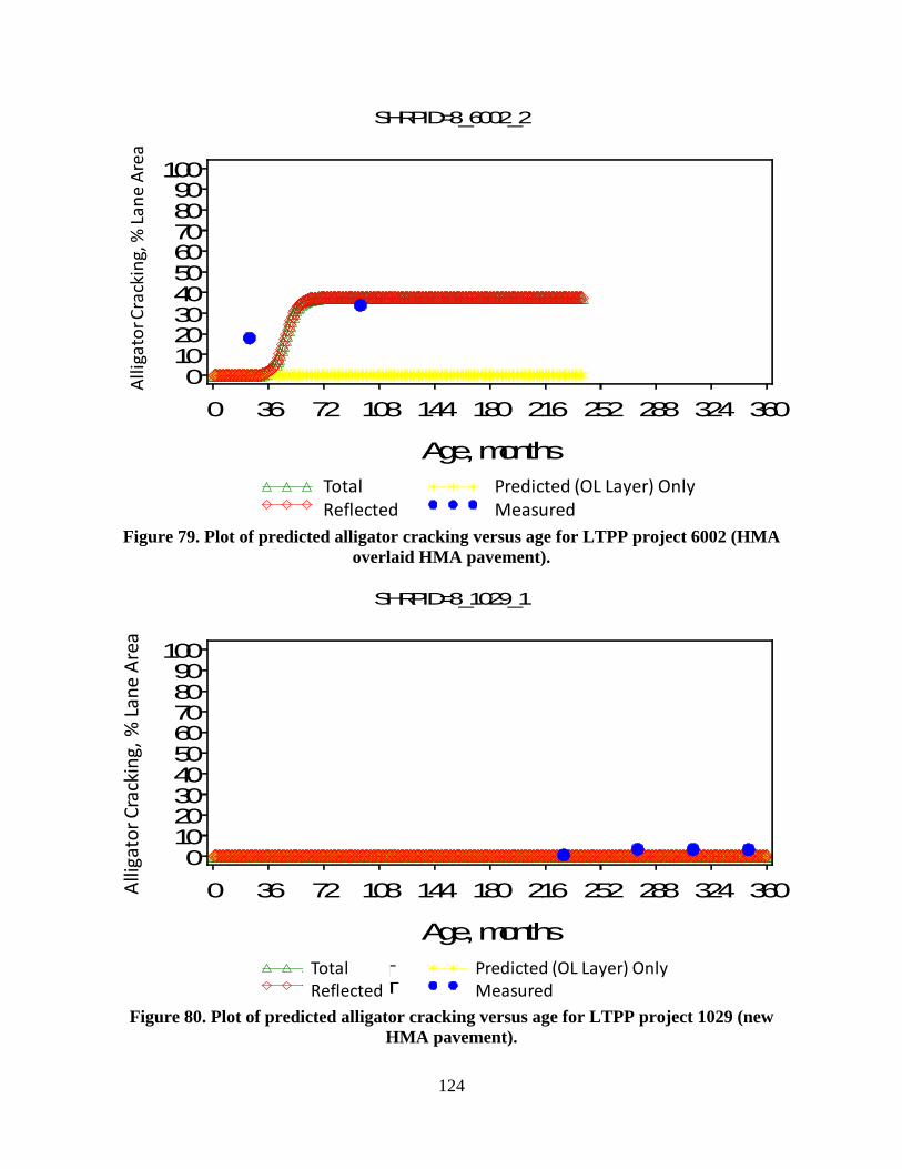
124

Figure 79. Plot of predicted alligator cracking versus age for LTPP project 6002 (HMA

overlaid HMA pavement).

Figure 80. Plot of predicted alligator cracking versus age for LTPP project 1029 (new

HMA pavement).

BU C

rack

ing, %

Ln A

rea

0102030405060708090

100

Age, months

0 36 72 108 144 180 216 252 288 324 360

SHRPID=8_6002_2

PLOTPREDICT BUONLYREFLECT LTPP AC

Predicted (OL Layer) OnlyMeasured

TotalReflected

Alligator Cracking, % Lan

e Area

BU C

rack

ing, %

Ln A

rea

0102030405060708090

100

Age, months

0 36 72 108 144 180 216 252 288 324 360

SHRPID=8_1029_1



TotalReflected

Alligator Cracking, % Lane Area

125

Figure 81. Plot of predicted alligator cracking versus age for CDOT pavement

management system project 13325.

Total Rutting Global MEDPG Total Rutting Model Verification The MEPDG predicts HMA pavement total rutting using separate submodels for the surface HMA, unbound aggregate base, and subgrade soil. The same three submodels are utilized for HMA-overlaid HMA pavement, with modifications as needed to reflect the existing pavement material properties and permanent strain (existing rutting) present in all three layers. Verification of the MEPDG global total rutting model consisted of the following steps:

1. Run the three MEPDG rutting submodels using global coefficients for all new HMA pavement and HMA-overlaid HMA pavement projects to obtain estimates of total rutting.

2. Perform statistical analysis to determine goodness of fit with field-measured total rutting and bias in estimated total rutting.

3. Evaluate goodness of fit and bias statistics and determine any need for local calibration to Colorado conditions.

Figure 82 shows a plot of the MEPDG global model predicted rutting versus field-measured rutting for all Colorado new HMA pavement and HMA-overlaid HMA pavement projects. Goodness of fit and bias statistics computed from the data are presented in Table 57.

BU C

rack

ing, %

Ln A

rea

0102030405060708090

100

Age, months

0 36 72 108 144 180 216 252 288 324 360

SHRPID=41-13325



TotalReflected

Alligator Cracking, % Lane Area

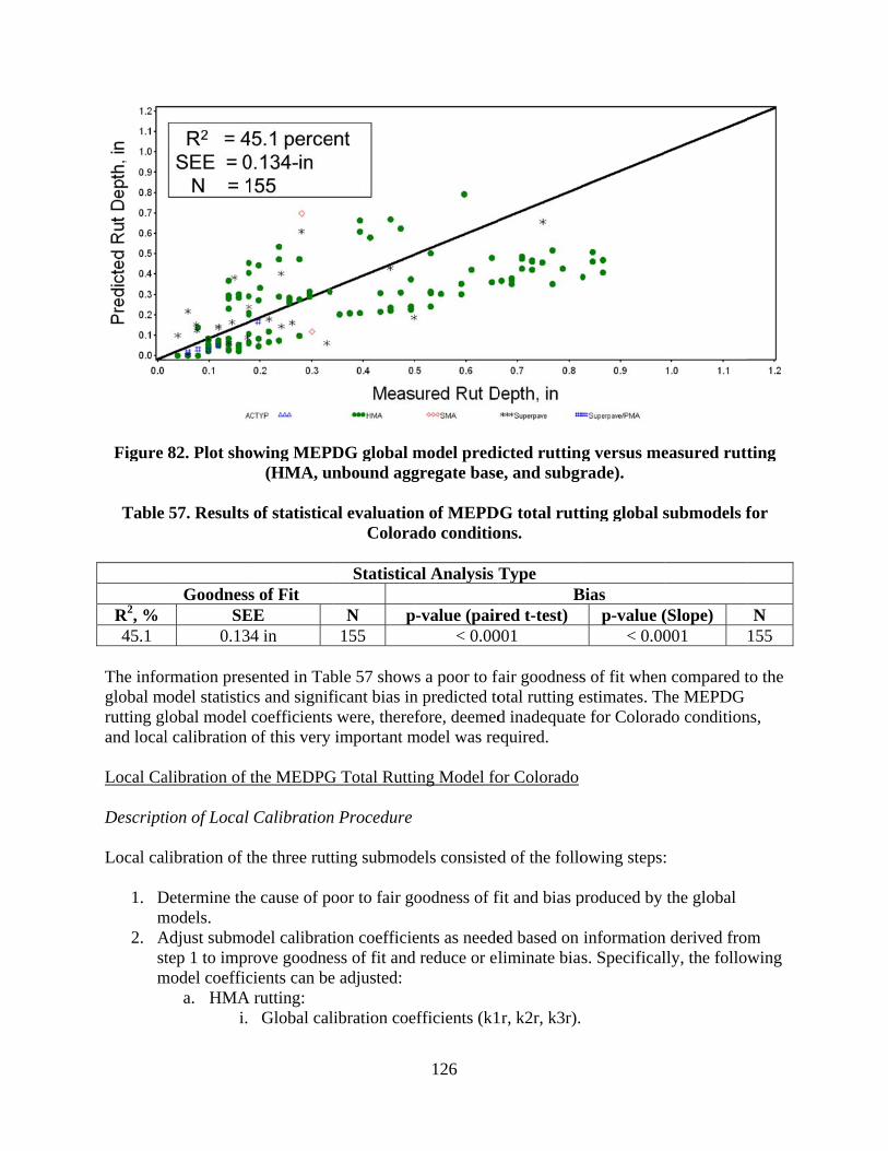
Figure

Table

R2, % 45.1

The inforglobal mrutting gland local Local Ca Descripti Local cal

1. Dm

2. Astm

82. Plot sho

57. Results

GoodnessSE

0.13

rmation presodel statisticlobal model l calibration

alibration of

ion of Local

libration of t

Determine themodels. Adjust submotep 1 to impr

model coeffica. HMA

i.

owing MEPD(HMA, u

of statistica

s of Fit EE

4 in

sented in Tabcs and signifcoefficientsof this very

the MEDPG

Calibration

the three rutt

e cause of po

odel calibratrove goodnecients can be

A rutting: Global cal

DG global mnbound agg

al evaluatioColora

Statistica

N p155

ble 57 showsficant bias in were, therefimportant m

G Total Rutti

n Procedure

ting submod

oor to fair go

ion coefficieess of fit ande adjusted:

libration coe

126

model predigregate base

n of MEPD

ado conditio

al Analysis

-value (pair< 0.00

s a poor to fan predicted tofore, deemed

model was re

ing Model fo

dels consisted

oodness of f

ents as needed reduce or el

efficients (k1

icted ruttine, and subgr

DG total ruttons.

Type B

red t-test) 001

fair goodnessotal rutting ed inadequateequired.

or Colorado

d of the follo

fit and bias p

ed based on liminate bia

1r, k2r, k3r).

g versus merade).

ting global s

Bias p-value (

< 0.00

s of fit whenestimates. The for Colorad

owing steps:

produced by

informations. Specifical

easured rutt

submodels f

(Slope) 001

n compared the MEPDG do condition

:

the global

n derived fromlly, the follow

ting

for

N 155

to the

ns,

m wing

127

ii. Local calibration coefficients (β1r, β2r, β3r). b. Granular base rutting model.

i. Local/global calibration coefficients (ks1). c. Subgrade rutting model.

i. Local/global calibration coefficients (ks1). In adjusting the three rutting submodels, the researchers considered information obtained through laboratory testing (repeated load permanent deformation and HWT tests) on the nature and rate of primary and secondary rutting development and from field trenching of new HMA pavements to determine the distribution of rutting within the pavement structure. This was done by (1) applying laboratory-derived HMA rutting submodel coefficients k1r, k2r, and k3r as seed values and constraining the new local models to be as close as possible to the seed values without compromising goodness of fit and bias and (2) ensuring that the contribution of each submodel to total rutting was close to the field trenching estimates without compromising goodness of fit and bias. A summary of laboratory-measured HMA rutting model coefficients k1r, k2r, and k3r and total rutting distribution is presented as follows:

Laboratory-measured HMA rutting model coefficients: o k1r = -2.36. o k2r = 1.72. o k3r = 0.16.

Total rutting distribution: o HMA surface = 63 percent. o Aggregate base/subbase = 11 percent. o Subgrade (top 12 in) = 26 percent.

Local calibration was done simultaneously for new HMA pavements and HMA-overlaid HMA pavements. Summary descriptions of the three rutting submodels are presented in Table 58. A detailed description of MEPDG rutting submodels is presented in Appendix A.

Table 58. Description of total rutting prediction submodels.

Model Type Model Description*

HMA rrrrr kkkHMArzrHMAHMApHMAp Tnkh 3322110)(1)()(

Unbound aggregate base

n

r

osoilvsssoilp ehk 11)(

Subgrade soils

n

r

osoilvsssoilp ehk 11)(

Summary of Total Rutting Model Local Calibration Results The researchers investigated the possible causes of poor goodness of fit and bias, and they found no obvious reasons (such as erroneous inputs). Thus, local calibration proceeded as previously described. Calibration of the MEPDG global models using CDOT input data was done using

128

nonlinear model optimization tools available in the SAS statistical software. Adjusted HMA rutting, unbound aggregate base rutting, and subgrade rutting global model coefficients obtained from step 2 are presented in Table 59 and show that three of the eight global coefficients were adjusted. The goodness of fit and bias statistics are presented in Table 60. A plot of field-measured versus CDOT-calibrated total rutting is presented in Figure 83. The goodness of fit and bias test results indicate an adequate goodness of fit with minimal bias not significant at the 5 percent significance level for the locally calibrated total rutting submodels. The results presented Table 60 also show no appreciable change in the goodness of fit between the global models and the Colorado calibrated models (i.e., R2 changed from 45.1 to 41.7 and SEE changed from 0.134 to 0.147 inches) with local calibration. Both the global and locally calibrated models goodness of fit was characterized as fair. The slight increase in SEE was attributed to high variability exhibited in field measurements of pavement rutting that contributes to lowering R2 and increasing SEE. The results presented Table 60 also show that the significant bias produced by the global models in Colorado had been eliminated through local calibration. This improvement increases overall rutting prediction accuracy and reliability of pavement designs. Thus, new HMA pavement and HMA-overlaid HMA pavement designs in Colorado will be much more accurate and optimum (lower cost) at the selected level of design reliability with the application of the locally calibrated total rutting model. Figures 84 through 88 present plots of measured and predicted rutting for several projects in Colorado. The plots show reasonable predictions of rutting using the locally calibrated models. Table 59. Local calibration coefficients for HMA, unbound base, and subgrade soil rutting

submodels.

Model Model

Coefficients Global Model

ValuesCDOT Local Model Values

HMA rutting submodel

Kr1 -3.35412 -3.35412 Kr2 1.5606 1.5606 Kr3 0.4791 0.4791 r1 1 1.34 r2 1 1 r3 1 1

Granular base rutting submodel

ks1 1 0.4

Subbase rutting submodel

ks1 1 0.84

Table 60

R2, % 41.7

Figure

Figure 8

RSN

0. Results of

GoodnessSE

0.14

83. Plot sho(f

84. Plot show

Rut Depth, in

0.0

0.1

0.2

0.3

0.4

0.5

0.6

0.7

0.8

0

R2 = 41.7 perSEE = 0.147N = 137

f statistical eloca

s of Fit EE 47 in

owing predicfor all pavem

wing high vma

0 24 4

rcent 7 in

evaluation oal models fo

Statistica

N p137

cted using Mments) vers

variation of anagement s

48 72

SHR

129

of MEPDG r Colorado

al Analysis

-value (pair0.430

MEPDG subsus field-me

measured rsystem proj

Age, mo

96 120

RPID=33-13435

alligator crconditions.

Type B

red t-test) 06

bmodels witasured tota

rutting overject 13435.

mo

144 168

5

racking and.

Bias p-value (

0.08

th CDOT loal rutting.

r time for C

192 216

d fatigue dam

(Slope) 98

ocal coeffici

DOT pavem

240

mage

N 137

ients

ment

130

Figure 85. Plot showing high variation of measured rutting over time for CDOT pavement


Figure 86. Plot showing high variation of measured rutting over time for CDOT pavement


Rut Depth, in

0.0

0.1

0.2

0.3

0.4

0.5

0.6

0.7

0.8

Age, mo

0 24 48 72 96 120 144 168 192 216 240

SHRPID=38-13505

Rut Depth, in

0.0

0.1

0.2

0.3

0.4

0.5

0.6

0.7

0.8

Age, mo

0 24 48 72 96 120 144 168 192 216 240

SHRPID=39-11970

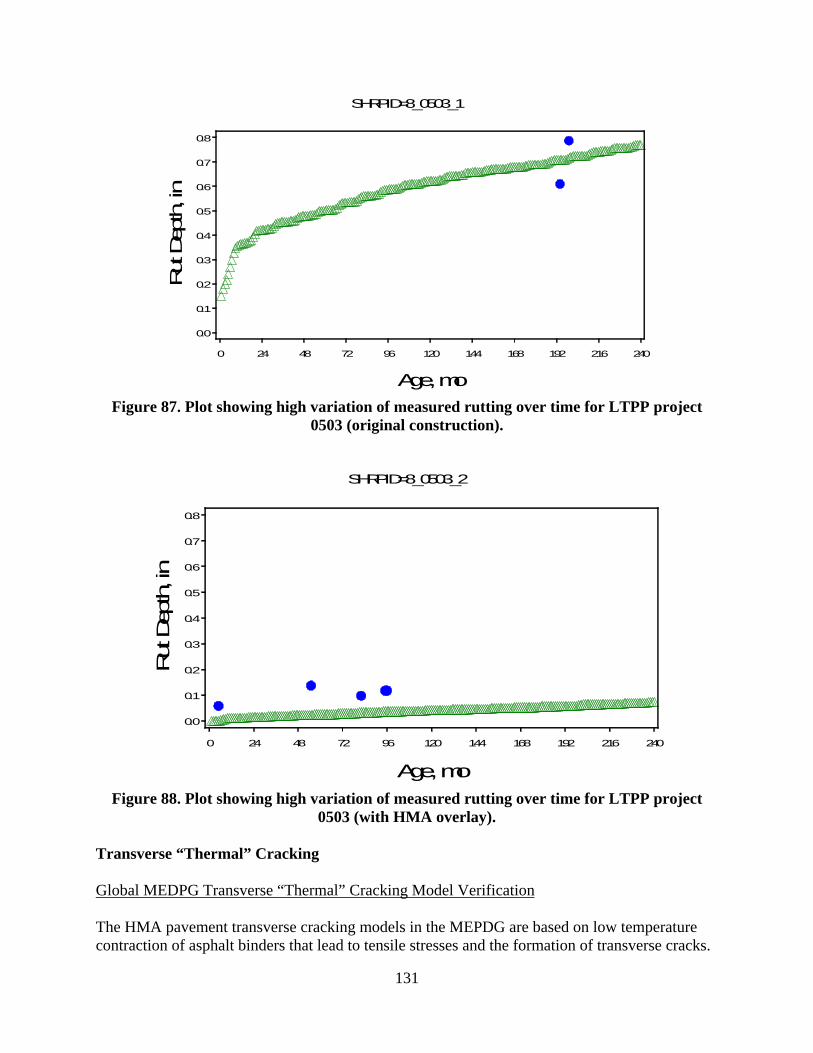
131

Figure 87. Plot showing high variation of measured rutting over time for LTPP project

0503 (original construction).

Figure 88. Plot showing high variation of measured rutting over time for LTPP project

0503 (with HMA overlay).

Transverse “Thermal” Cracking Global MEDPG Transverse “Thermal” Cracking Model Verification The HMA pavement transverse cracking models in the MEPDG are based on low temperature contraction of asphalt binders that lead to tensile stresses and the formation of transverse cracks.

Rut Depth, in

0.0

0.1

0.2

0.3

0.4

0.5

0.6

0.7

0.8

Age, mo

0 24 48 72 96 120 144 168 192 216 240

SHRPID=8_0503_1

Rut Depth, in

0.0

0.1

0.2

0.3

0.4

0.5

0.6

0.7

0.8

Age, mo

0 24 48 72 96 120 144 168 192 216 240

SHRPID=8_0503_2

132

In general, transverse cracking is expected to be more severe in very cool climate zones than in warmer areas. Colorado’s climate is segmented into four zones (see Table 61) ranging from the very cool high elevations (> 8500 ft) to the moderate to hot lower elevations (< 6000 ft).

Table 61. Colorado environmental zones.

CDOT Environmental Zone Highest 7-Day Average Maximum Air Temperature, °F Hot (Southeast and West) > 97

Moderate (Denver, Plains, and West) 90 to 97 Cool (Mountains) 81 to 88

Very cool (High Mountains) < 81 The MEPDG HMA transverse cracking models is presented below:

HMA

d

d H

CLogNKTC

1

(11)

Key inputs required by the MEPDG HMA transverse cracking model include HMA creep compliance and indirect tensile strength. The key inputs can be measured at Level 1 or estimated based on HMA mixture volumetrics and aggregate properties (Level 3). Because of the sensitivity of the MEPDG HMA transverse cracking model to these inputs, it is recommended that only Level 1 HMA creep compliance and indirect tensile strength inputs be used for local calibration. Thus, the following MEPDG HMA transverse cracking model verification was done using only projects with Level 1 data:

1. Identify HMA projects with Level 1 HMA creep compliance and indirect tensile strength data. Twelve projects were used for verification, and they exhibited a wide range of transverse cracking after approximately 10 years in service.

2. Run the MEPDG with the global coefficients for all 12 projects. 3. Perform statistical analysis to characterize goodness of fit and bias. 4. Evaluate goodness of fit and bias, summarize the outcome, and develop

recommendations for local calibration.

The outcome of the MEPDG runs for all of the HMA sections using the global calibration coefficients for Level 1 (e.g., K = 1.5) is presented in Table 62. Figure 89 shows a plot of the MEPDG global transverse cracking model-predicted transverse cracking versus field-measured transverse cracking. This information shows that using the MEPDG global transverse cracking model in Colorado produces biased estimates (under-prediction) and a poor goodness of fit. Thus, there was the need for local calibration of the MEPDG global transverse cracking model.

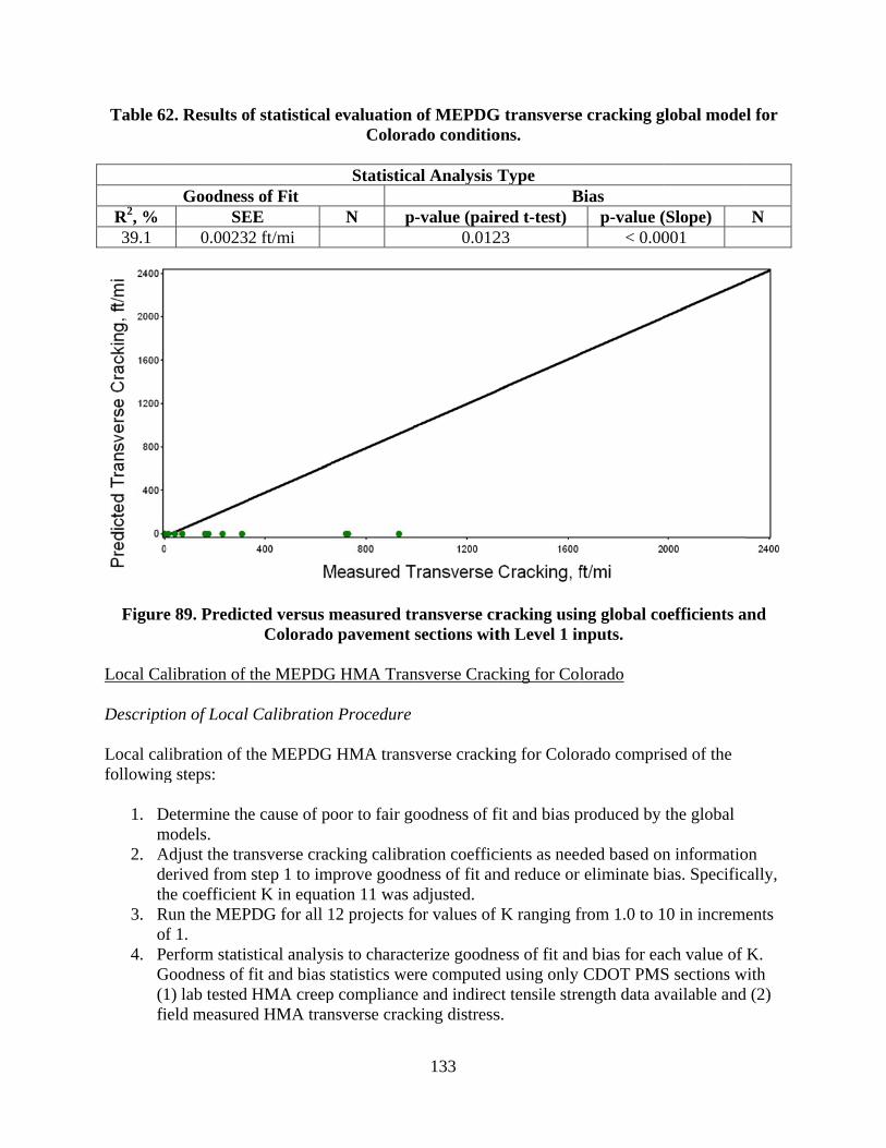
Table 6

R2, % 39.1

Figure

Local Ca Descripti Local calfollowing

1. Dm

2. Adth

3. Ro

4. PG(1fi

2. Results o

GoodnessSE

0.0023

e 89. Predic

alibration of

ion of Local

libration of tg steps:

Determine themodels. Adjust the tra

erived from he coefficien

Run the MEPf 1. erform statis

Goodness of 1) lab tested ield measure

of statistical

s of Fit EE 2 ft/mi

cted versus mColorado

the MEPDG

Calibration

the MEPDG

e cause of po

ansverse cracstep 1 to im

nt K in equatPDG for all 1

stical analysfit and bias sHMA creep

ed HMA tran

evaluation Colora

Statistica

N p

measured tro pavement

G HMA Tran

n Procedure

G HMA trans

oor to fair go

cking calibramprove goodn

tion 11 was a12 projects fo

is to charactstatistics wer

p compliancensverse crack

133

of MEPDGado conditio

al Analysis

-value (pair0.012

ransverse crsections wit

nsverse Crac

sverse cracki

oodness of f

ation coefficness of fit anadjusted.

for values of

terize goodnre computede and indirecking distress

G transverseons.

Type B

red t-test) 23

racking usinth Level 1 in

cking for Col

ing for Color

fit and bias p

cients as neednd reduce or

f K ranging f

ness of fit andd using only ct tensile stres.

e cracking g

Bias p-value (

< 0.00

ng global conputs.

lorado

rado compri

produced by

ded based oneliminate bi

from 1.0 to 1

d bias for eaCDOT PMS

ength data av

global mode

(Slope) 001

oefficients a

ised of the

the global

n informatioias. Specific

10 in increm

ach value of S sections wvailable and

l for

N

and

on cally,

ents

K. with d (2)

5. Eg

Summary Coefficiecracking cracking cracking CDOT logoodnessat the 5 presults prbetween to 43.1 pSEE for b

Mo

HMA tracrack

Figurethe ME

Evaluate goodoodness of f

y of HMA Tr

ent K = 7.5 pgenerally mK coefficienfor all 12 C

ocally calibras of fit and bpercent signiresented Tabthe global mercent). Eveboth the glob

Table

odel C

ansverse king

e 90. Plot shEPDG mode

dness of fit afit and least b

ransverse Cr

produced thematched field

nts are preseDOT PMS sated model g

bias test resuificance leveble 64 also inmodel when aen though SEbal and loca

e 63. Local c

Model Coefficients

K

owing predel with CDO

and bias andbias.

racking Mod

e best goodnd-measured vented in Tablsections usedgoodness of lts indicates

el for the locandicates conapplied in C

EE increasedlly calibrated

calibration c

s Global M

icted versusOT local coe

from pro

134

d select the v

del Local Ca

ess of fit andvalues). The le 63. A plotd in local calfit and bias an adequate

ally calibratesiderable imolorado and

d for 0.002 ftd models we

coefficients

Model Value

1.5

s measured efficients an

oject field te

value of K va

alibration Re

d minimal biglobal and l

t of predictedlibration is pstatistics are

e goodness oed transvers

mprovement id the locally ct/mi to 194 fere character

for transve

e CDOT

transverse nd HMA traesting.

alue that pro

esults

ias (i.e., predlocally calibd versus meapresented in e presented iof fit with ine cracking min the goodncalibrated mft/mi with lorized as adeq

erse crackin

T Local Mo

7.5

cracking deansverse cra

oduces the be

dicted transvrated transveasured transFigure 90. T

in Table 64. significant b

model. The ness of fit

model (i.e., 39cal calibratioquate.

ng.

del Value

eveloped usacking distr

est

verse erse verse

The The

bias

9.1 on,

sing ress

Table 6

R2, % 43.1

The CDOmeasuredpredictedpresentedresults pr

FigureMEPD

Table 6

R2, % 44.4

The resulmodels htransversFigures 9projects ilocally ca

64. Results o

GoodnessSE

194 f

OT locally cad HMA transd versus mead in Figure 9resented wer

e 91. Plot shDG model w

65. Results oColorad

GoodnessSE

178 f

lts presentedhad been elimse cracking p92 through 9in Colorado.alibrated mo

of statistical

s of Fit EE ft/mi

alibrated HMsverse crackasured transv91, and goodre deemed re

owing predwith CDOT

of statisticaldo condition

s of Fit EE ft/mi

d in Table 64minated throuprediction ac97 present plo. The plots shodels.

l evaluationColora

Statistica

N p12

MA transversking data avaverse crackindness of fit aneasonable.

icted versuslocal coeffi

d

l evaluations using mea

Statistica

N p37

4 and 65 shough local ca

ccuracy and rots of measuhow reasona

135

n of MEPDGado conditio

al Analysis

-value (pair0.529

se cracking mailable in theng for all 12 nd bias stati

s measured cients and mdistress.

n of MEPDGasured HMA

al Analysis

-value (pair0.698

ow that the sialibration. Threliability ofured and preable predicti

G transversons.

Type B

red t-test) 90

model was fe CDOT PM

sections usestics are pre

transverse measured H

G transversA transvers

Type B

red t-test) 82

ignificant bihis improvemf HMA pavedicted transv

ions of transv

e cracking l

Bias p-value (

0.33

further validaS database. ed in local casented in Ta

cracking deHMA transv

e cracking lse cracking d

Bias p-value (

0.26

as producedment increasement designverse crackinverse crackin

local model

(Slope) 90

ated using A plot of alibration is able 65. The

eveloped usverse cracki

local model data.

(Slope) 60

d by the globses overall ns in Coloradng for severang using the

for

N 12

sing ng

for

N 37

bal

do. al

e

Figure 9

Figure 9

92. Plot shofo

93. Plot shofo

wing predicr CDOT pa


cted and meavement ma


136

easured trananagement s


nsverse cracsystem proje


cking versuect 13131.


us pavement

us pavement

t age

t age

Figure 9

Figure 9

94. Plot shofo

95. Plot shofo





137







us pavement

us pavement

t age

t age

Figure 9

Figure 9

Smoothn Global M Verificatmodel foall projecmeasuredshown in

96. Plot shofo

97. Plot shofo

ness

MEDPG HM

tion of the Mor Colorado ccts and evalud IRI for all n Table 66.



MA Smoothne

MEPDG globconditions couating goodnrelevant pav



ess Model V

bal new HMAonsisted of rness of fit anvement proje

138



Verification

A pavement running the Mnd bias. Figuects. Goodne



and HMA-oMEPDG wit

ure 98 showsess of fit stat



overlaid HMth the globals a plot of pretistics and bi

us pavement

us pavement

MA pavemenl coefficientsedicted versias statistics

t age

t age

t IRI s for us are

Figur

Table 6

R2, % 35.5

The goodpredictiocalibratio

Local Ca Descripti Local cal

1. Dm

2. Afradeqloel

re 98. Predic

6. Results o

GoodnessSEE, 15.9 i

dness of fit sns are biased

on of this ver

alibration of

ion of Local

libration of t

Determine themodels. Adjust the glorom step 1 todjusting the quation 12) uocal calibratiliminates bia

cted versus Colorad

of statistical

s of Fit in/mi in/mi

statistics are d (the modelry important

the MEPDG

Calibration

the MEPDG

e cause of po

obal model co improve goMEPDG HMusing nonlinion coefficieas.

measured Ido HMA pa

evaluation co

Statistica

N p343

poor, and thl overpredictt model was

G HMA Smo

n Procedure

G HMA IRI m

oor to fair go

calibration coodness of fiMA IRI modnear optimizaents that max

139

IRI using glavement per

of MEPDG

onditions.

al Analysis

-value (pair0.553

he hypothesists IRI for higrequired.

oothness Mo

model for Co

oodness of f

oefficients afit and reducedel global caation algoritximizes good

lobal MEPDrformance d

G HMA IRI

Type B

red t-test) 30

s test resultsgher measur

odel for Colo

olorado cons

fit and bias p

as needed bae or eliminat

alibration coethms in SASdness of fit a

DG HMA IRdata.

global mod

Bias p-value (

< 0.00

s indicate thered IRI value

orado

sisted of the

produced by

ased on inforte bias. Thisefficients (C

S to produce and significa

RI model an

del for Color

(Slope) 001 3

e global modes). Thus, lo

following st

the global

rmation derivs involved C1 through C

a new set ofantly reduces

nd

rado

N 343

del cal

teps:

ved

C4 in f s or

140

3. Perform statistical analysis (using SAS) to characterize goodness of fit and bias for the new local coefficients.

4. Evaluate goodness of fit and bias and summarize outcome. 5. Repeat steps 2 to 4 as needed until goodness of fit and bias are acceptable.

RDCTCCFCCSFCIRIIRI Totalo 4321 (12)

Where all inputs are as already defined. Summary of HMA Smoothness Model Local Calibration Results

The new local calibration coefficients for the HMA smoothness model for Colorado are presented in Table 67. Goodness of fit and bias statistics for the locally calibrated HMA smoothness model are presented in Table 68. A plot of measured and predicted IRI for new HMA pavements and HMA-overlaid existing HMA pavements is presented in Figure 99. The information presented in Table 68 indicates a large improvement in the goodness of fit between the global HMA smoothness model and the Colorado locally calibrated HMA smoothness model (i.e., R2 after calibration was 64.4 percent, compared to a pre-calibration value of 35.5 percent). SEE increased marginally from 15.9 to 17.2 in/mile, which was considered fair. Hypothesis testing to determine the presence or absence of significant bias indicated that the locally calibrated model predictions were not significantly biased (at the 5 percent significance level). Thus, the significant bias present in the global model IRI predictions for Colorado has been eliminated.

Table 67. Local calibration coefficients for HMA smoothness (IRI) model.

Model Coefficients CDOT Local Model Values

Global Model Values

C1 (for rutting) 35 Yes

C2 (for alligator cracking) 0.3 Yes

C3 (for transverse cracking) 0.02 Yes

C4 (for site factor) 0.019 Yes

Table 68. Results of statistical evaluation of MEPDG HMA IRI local model for Colorado conditions.

Statistical Analysis Type

Goodness of Fit Bias R2, % SEE, in/mi N p-value (paired t-test) p-value (Slope) N 64.4 17.2 343 0.1076 0.3571 343

Figure

Figure 10impact ofpavemenaccurate

Figure 1

e 99. Plot ofpavements

00 through 1f local calibr

nt designs baand optimum

00. Plot sho

IRI, in

/mi

0

24

48

72

96

120

144

168

192

216

240

f measured developed

102 illustrateration is mos

ased in part om (lower cos

owing measu

0 36

and predictusing the lo

e the model Ist significanton HMA pavst) at the sele

ured and pr

72 108

SHRPID

141

ted IRI for nocally calibr

IRI predictiot in removin

vement IRI inected level o

redicted IRI

Age, mon

144 180

D=32-12448_ca

new HMA arated CDOT

on for typicang the large un Colorado w

of design reli

I versus tim

nths

216 252

calib

and HMA-oT HMA IRI

al HMA paveunder-predicwill thus be iability.

me for CDOT

288 324

overlaid HMI model.

ements. Thection bias. Hmuch more

T project 12

360

MA

e HMA

2448.

142

Figure 101. Plot showing measured and predicted IRI versus time for CDOT project 13435.

Figure 102. Plot showing measured and predicted IRI versus time for CDOT project 12685. Estimating Design Reliability for New HMA and HMA Overlay Pavement Distress Models The MEPDG estimates pavement design reliability using estimates of distress and IRI standard deviation for any given level of predicted distress or IRI. Thus, for each of the 3 HMA pavement distress models, there was a need to develop a relationship between predicted distress and the predictions standard error. Predicted distress standard error prediction equations were developed as follows:

1. Divided predicted distress into 3 or more intervals.

IRI, in

/mi

0

24

48

72

96

120

144

168

192

216

240

Age, months

0 36 72 108 144 180 216 252 288 324 360

SHRPID=33-13435

IRI, in

/mi

0

24

48

72

96

120

144

168

192

216

240

Age, months

0 36 72 108 144 180 216 252 288 324 360

SHRPID=8-12685

143

2. For each interval, determine mean predicted distress and standard error (i.e., standard variation of predicted – measured distress for all the predicted distress that falls within the given interval).

3. Develop a non linear model to fit mean predicted distress and standard error for each interval.

The resulting standard error of the estimated distress models developed using the locally calibrated CDOT HMA distress models are presented below:

)log10(DAM)*2.4656--1.6673(1

151)(

eGATORSEE

(12)

001.0*2052.0)( 4.0 ACRUTACRUTSEE (13)

001.0*2472.0)( 67.0 BASERUTBASERUTSEE (14)

001.0*1822.0)( 5.0 SUBRUTSUBRUTSEE (15)

027.65*1468.0)( TRANSTRANSSEE (16)

where

SEE(GATOR) = alligator cracking standard deviation, percent lane area SEE(TRANS) = transverse cracking standard deviation, ft/mi SEE(ACRUT) = HMA layer rutting standard deviation, in SEE(BASERUT) = base layer rutting standard deviation, in SEE(SUBRUT) = subgrade layer rutting standard deviation, in DAM = alligator cracking fatigue “bottom-up” damage TRANS = predicted HMA transverse cracking, ft/mi ACRUT = predicted HMA layer rutting, in BASERUT = predicted base layer rutting, in SUBRUT = predicted subgrade layer rutting, in

Note that smoothness (IRI) standard error is estimated internally by the MEPDG.

144

CHAPTER 7. VERIFICATION AND CALIBRATION OF RIGID PAVEMENTS This chapter describes work done to verify and calibrate, if needed, the MEPDG global rigid pavement distress and smoothness models for Colorado. For this project, rigid pavements include new JPCP and unbonded JPCP overlay over existing JPCP. The criteria for performing local calibration were based on whether the given global model exhibited a reasonable goodness of fit (between measured and predicted outputs) and whether distresses/IRI were predicted without significant bias. Reasonable goodness of fit was determine using R2 and SEE, while the presence or absence of bias was determined based on the hypothesis test described in chapter 3. The general criteria used to determine global model adequacy for Colorado conditions are presented in Table 69. Table 70 lists the rigid pavement models evaluated as part of the MEPDG implementation in Colorado. Detailed descriptions of these models are presented in Appendix A.

Table 69. Criteria for determining global models adequacy for Colorado conditions.

Criterion of Interest

Test Statistic Range of R2, percent

& SEE of Models Rating

Goodness of fit

Coefficient of determination (R2), percent (all models)

81 to 100 Very good (strong relationship) 64 to 81 Good 49 to 64 Fair

< 49 Poor (weak or no relationship)

Global JPCP transverse cracking model SEE

< 4.5 percent Good 4.5 to 9 percent Fair

> 9 percent Poor

Global JPCP transverse joint faulting model SEE

< 0.033 in Good 0.033 to 0.066 in Fair

> 0.066 in Poor

Global JPCP IRI model SEE < 17 in/mi Good

17 to 34 in/mi Fair > 34 in/mi Poor

Bias

Hypothesis testing of slope of the linear measured vs.

predicted distress/IRI model (b1 = slope) H0: b1 = 0

p-value Reject if p-value is < 0.05 (i.e., 5

percent significant level)

Paired t-test between measured and predicted

distress/IRI p-value

Reject if p-value is < 0.05 (i.e., 5 percent significant level)

145

Table 70. MEPDG rigid pavement global models evaluated for Colorado local conditions.

Pavement Type MEPDG “Global” Models Evaluated

JPCP Transverse Cracking

JPCP Transverse Joint Faulting

New JPCP IRI

New JPCP Unbonded overlay over existing JPCP

New JPCP and Unbonded JPCP Overlays Transverse Cracking Model Global MEDPG JPCP Transverse “Mid-Panel Slab” Cracking Model Verification Figure 103 presents a histogram of all measured (including time series) transverse “mid-panel slab” cracking for the CDOT pavement management system and LTPP projects included in the analysis. The figure shows a limited distribution of transverse cracking data, with most of the measured cracking being zero. Thus, commonly applied statistical procedures could not be used to characterize the model’s goodness of fit and bias under Colorado conditions. The project team, therefore, applied a mostly non-statistical analysis procedure to verify the suitability of the MEPDG global transverse cracking model for Colorado conditions. The non-statistical goodness of fit and bias characterization procedure consisted of the following:

Comparison of grouping of measured and predicted transverse cracking (grouped using engineering judgment into as many groupings as needed) to determine how often measured and predicted transverse cracking remained in the same group. Measured and predicted transverse cracking remaining in the same group implied reasonable goodness of fit and insignificant bias, while measured and predicted transverse cracking residing in different groups suggested otherwise.

Comparison of distribution of residual (predicted – measured transverse cracking) to determine reasonableness of predictions. Basically, predicted transverse cracking that falls with 2 standard deviations of measured transverse cracking is deemed reasonable (i.e., predicted transverse cracking must fall within measured transverse cracking + 2*SEE). A significant majority of data falling within the range of measured transverse cracking + 1*SEE indicates very little bias.

Apply the non-parametric Chi-square (χ2) test to characterize and evaluate goodness of fit and bias between observed and predicted transverse cracking data.

Verification of the MEPDG global JPCP transverse cracking model for Colorado conditions began by running the MEPDG analysis for all JPCP projects. For this analysis, the NCHRP Project 20-07(288) JPCP MEPDG global model coefficients were applied, since these coefficients are compatible with CDOT and LTPP revised PCC CTE data used in transverse cracking predictions. The outcomes of the analyses are presented in the following sections.

Figure 1

Summary Compari For this cTable 71in the samdata avai71 showe

Aan

Tm

Fpr

Figure 10age for JPin agreem

103. Histogrfo

y of JPCP Tr

son of Meas

comparison, . The goal wme groupingilable and used the follow

Approximatend predicted

Three percentmeasured gro

or the remairedictions fe

04 shows a pPCP project

ment with the

ram showinor CDOT a

ransverse Cr

sured and Pre

transverse “was to determg. The range sing engineerwing:

ly 87 percend alligator crat of the data

ouping 2 to 5ining two daell into predi

plot of measus using MEPe trends repo

ng distributind LTPP pr

racking Veri

edicted Tran

“slab” crackimine how oft

of each grouring judgme

nt of all data acking grouppoints (23 o

5 against preata points, foicted groupin

ured and prePDG global torted in Tabl

146

ion of measurojects inclu

ification Res

nsverse Crac

ing was cateten measuredup was deternt. A review

points (218ping (0 to 2

of 249) fell wdicted groupr measured gngs 0 to 2.

edicted transtransverse crle 71.

ured JPCP uded in the

sults

cking Groupi

egorized intod and predicrmined based

w of the infor

of 249) fell percent crac

within an adjping 0 to 2).groupings 5

sverse “slab”racking mod

transverse analysis.

ings

o four groupscted transverd on the distrmation pres

within the scking). jacent group

to 10, the M

” cracking vedel coefficien

“slab” crac

s, as shown irse cracking tribution of tsented in Tab

same measur

ping (i.e.,

MEPDG

ersus pavemnts. The plot

cking

in fell the ble

red

ment t is

Table 7

Meas

C

Figu

pav

Evaluatio Figure 10cracking)all the repoints wethe predi

71. Compar

ured TransveCracking, perc

0-2 2-5

5-10 > 10

ure 104. Plotvement age

on of Distrib

05 shows a d) for all 246 siduals fell were all withinctions from

rison of mea

rse Slab cent

t showing mfor JPCP p

bution of Res

distribution odata points

within 1 SEEn 2 SEE of tactual measu

asured and mea

MEP0-2 218 23 8 0

measured anrojects usin

co

siduals

of residuals included in tE of the meathe measuredured transve

147

predicted trasurements)

PDG Predicted2-50 0 0 0

nd predictedng MEPDG oefficients.

(predicted –the analysis.

asured transvd transverse erse cracking

ransverse c).

d Transverse

d transverseglobal tran

– measured p. The plot shverse crackincracking val

g were deem

racking (pe

Slab Cracking5-10

0 0 0 0

e “slab” cransverse crac

percent slab whows that ovng value. Thlue. Thus, de

med good or f

ercentage of

g, percent>10

0 0 0 0

cking versuking model

with transveer 90 percen

he remaining eviations of fair.

f all

us

erse nt of

data all

Figure 1

Statistica Statisticasample opredictedcracking percent). A hypothcracking will fall i

1. D2. F3. P

4. Enu0

The resul

Dfrdo

105. Plot shtransver

al Chi-square

al χ2 testing wof measured td transverse into several

hesis was forfall in the 0

in the same b

Determine meormulate hyerform analy

a. Calcub. Determc. Comp

Evaluate statiull hypothes.05, represen

lts of the χ2 t

Determine therequency disividing the rccurrences i

owing distrrse cracking

e Testing to

was performtransverse slslab crackinl bins (e.g., th

rmulated andto 2 percent

bin. The χ2 s

easured tranypothesis. ysis.

ulate the χ2 temine test de

pare the χ2 teistical test resis is rejectednting a 95 pe

test are prese

e frequency stribution of range of trann the given b

ribution of rg) for all 246

Characterize

med to test thelab crackingg were similhree bins wi

d tested that t bin, then a statistical ana

nsverse crack

est statistic.grees of free

est statistic toesults and ded only whenercent signif

ented as foll

distribution the measure

nsverse crackbins. Becaus

148

residuals (pr6 observatio

e Goodness

e hypothesisg (246 data plar. This wasith transvers

states that ifsimilar percalysis proced

king frequen

edom. o the criticaletermine when p-value is leficance level

lows:

of measureded transverseking values ise of the ske

redicted – mons included

of Fit and B

s that the disoints) and ths done by die cracking v

f X percent ocentage of prdure consist

ncy distributi

l χ2 value to ether to rejecess than pre-l.

d transverse e cracking dainto bins andewed distribu

measured ped in the ana

Bias

stribution of he distributioividing measvalues 0 to 2

of measuredredicted tranted of the fol

ion.

estimate p-vct the null hy-determined

cracking daata was deted correspondution of the m

ercent slab walysis.

the random on of MEPDsured transve, 2 to 4, and

d transverse nsverse crackllowing step

value. ypothesis. T

d level, usual

ata. The ermined by ding number measured

with

DG erse > 4

king s:

he lly

r of

149

transverse cracking data, the data could practically only be divided into two bins (zero and non-zero transverse cracking measurements). The distribution of measured transverse cracking into the two bins is presented in Table 72.

Formulate hypothesis. The hypothesis assumed for statistical testing is presented below: o H0: The percentages of predicted transverse cracking for the bins described in

Table 72 is similar to that observed for measured transverse cracking (Bin A: 84%, Bin B: 16%).

o HA: The percentages of predicted transverse cracking for the bins described in Table 72 is NOT similar to that observed for measured transverse cracking (Bin A: 84%, Bin B: 16%).

Perform analysis. The results of the χ2 testing are presented below: o χ2 = 0.0211, degrees of freedom = 1, and sample size = 249. o p-value (Pr > χ2) = 0.8845.

Evaluate statistical test results and determine whether to reject the null hypothesis. At the 95 percent significant level, the statistical χ2 results indicate no significant difference in measured and predicted transverse cracking data. Thus, the null hypothesis was accepted. This implies that the global MEPDG transverse “slab” cracking model performed reasonably well for Colorado conditions and local calibration was not warranted at this stage. However, because this evaluation was done using projects in relatively good condition with little or no cracking, it will be necessary to observe this model in the future to determine how well it predicts cracking once the JPCP projects used in the analysis start deteriorating. This can be done through continuous monitoring of the selected projects.

Table 72. Frequency distributions of measured transverse cracking data.

Bins Frequency Percent Cumulative Frequency

Cumulative Percent

A (0 to 0.2 percent)

209 84 209 84

B (> 0.2 percent)

40 16 249 100

Figures 106 through 108 illustrate the transverse fatigue cracking model for selected projects.

Figure 1LTPP

Figure 1LTPP 4_

106. Plot of 4_0213 (us

107. Plot of _0217 (usin

predicted aing global c

predicted ang global cal

and measurecalibration f

base

and measurelibration fac

base

150

ed transverfactors and friction age

ed transverctors and refriction age

rse crackingrecommend

e).

rse crackingecommendee).

g versus fatided loss of s

g versus fatied loss of sla

gue damageslab/aggrega

gue damageab/lean conc

e for ate

e for crete

Figure 1Colo

New JPC Global M Figure 10for the Cinformatifaulting djoint faulevaluate as describtransvers Verificatconsistedall selectmodel corevised Pare prese

108. Plot of orado JPCP

CP and Unb

MEDPG JPC

09 presents aDOT pavemion provideddata, with mlting was mogoodness ofbed for JPCP

se joint faulti

tion of the Md of the runned projects.

oefficients wPCC CTE daented in the f

predicted aP 54-11546 (u

sl

bonded JPC

P Transvers

a histogram ment managed in the figur

most of the mostly zero, cof fit and biasP transverse ing model fo

MEPDG globning the MEP

For this anawere applied, ata used in trfollowing sec

and measureusing globalab/aggrega

CP Overlays

e Joint Fault

of all measument systemre shows a lieasured faulommonly ap. The projeccracking to

or local Colo

bal JPCP tranPDG analysialysis, the NC

since these ansverse joinctions.

151

ed transveral calibrationate base frict

s Transverse

ting Model V

ured (includim and LTPP imited distriblting being zpplied statistict team thus a

verify the suorado conditi

nsverse jointis with the gCHRP Projecoefficients nt faulting p

rse crackingn factors antion age).

e Joint Faul

Verification

ng time seriprojects inclbution of me

zero. Becausical proceduapplied the suitability of ions. The pr

t faulting molobal transvect 20-07(288are compati

predictions. T

g versus fatind recomme

lting Model

es) transversluded in the easured transe the measur

ures could nosame non-stathe MEPDG

rocedures are

odel for Coloerse joint fau8) JPCP MEible with CDThe outcome

gue damageended loss o

l

se joint faultanalysis. Th

sverse joint red transversot be used toatistical met

G global e as follows:

orado conditulting model

EPDG globalDOT and LTes of the ana

e for of

ting he

se o thods

:

tions l for l

TPP alyses

Figure 1

CDO Summary Compari For this cThe goalgroupingand using

Table 7

Mea

Jo

A review

Aan

Sgr

FM

109. HistogrOT paveme

y of JPCP Tr

son of Meas

comparison, was to deter

g. The range g engineerin

73. Compari

asured Tranoint Faulting

0 to 0.03 0.03 to 0.0

> 0.06

w of the infor

Approximatend predictedix percent orouping 0.03or the remai

MEPDG pred

ram showingent managem

ransverse Fa

sured and Pre

transverse frmine how oof each grou

ng judgment.

ison of mea

nsverse g, in

6

rmation pres

ly 92 percend transverse jf the data po3 to 0.06 againing 2 percedictions fell i

g distributioment system

aulting Verif

edicted Tran

faulting was often measurup was deter

sured and pall me

MEPD0 to 0.03

151 9 3

sented in Tab

nt of all data joint faultingoints (9 of 16ainst predicteent of data pin predicted

152

on of measum and LTPP

fication Resu

nsverse Fault

categorized red and predrmined based

predicted treasurements

DG Predicte3

ble 73 showe

points (151g grouping (63) fell withied grouping oints belonggrouping 0

ured JPCP tP projects in

ults

ting Groupin

d into four grdicted transvd on the dist

ransverse jos).

ed Transver0.33 to 0.0

0 0 0

ed the follow

of 163) fell (0 to 0.03 in in an adjacen0 to 2).

ging to measto 0.03.

transverse jncluded in t

ngs

roups, as shoerse faultingtribution of t

oint faulting

rse Joint Fau06

wing:

within the sfaulting). nt grouping

sured groupin

joint faultinthe analysis.

own in Tableg fell in the sthe data avai

g (percentag

ulting, in> 0.06

0 0 0

same measur

(i.e., measur

ng > 0.06,

ng for .

e 73. same ilable

ge of

red

red

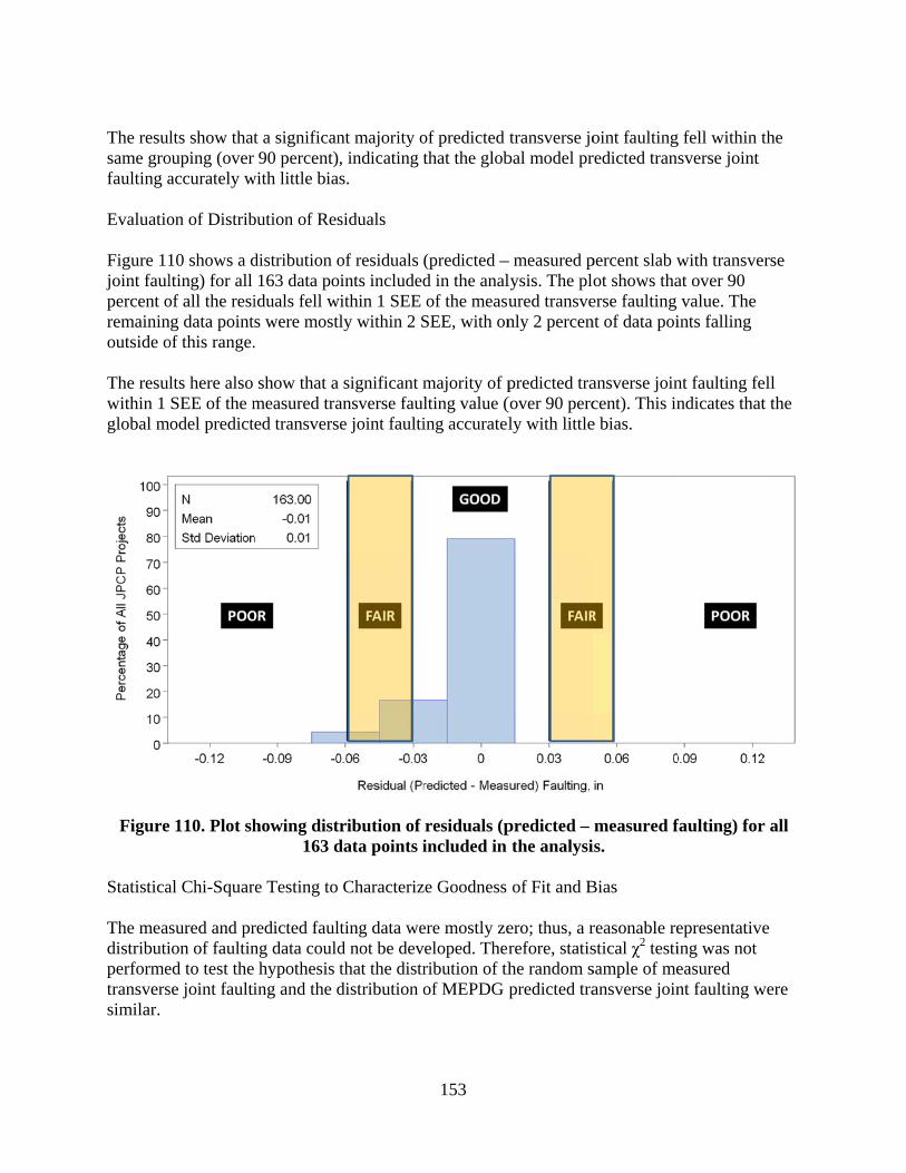
The resulsame grofaulting a Evaluatio Figure 11joint faulpercent oremaininoutside o The resulwithin 1 global m

Figure

Statistica The measdistributiperformetransverssimilar.

lts show thatouping (over accurately w

on of Distrib

10 shows a dlting) for all of all the resing data pointof this range.

lts here also SEE of the model predict

110. Plot sh

al Chi-Squar

sured and prion of faultined to test these joint faulti

t a significan90 percent)

with little bia

bution of Res

distribution o163 data po

iduals fell ws were most.

show that a measured traed transvers

howing dist163 d

re Testing to

redicted faulng data could hypothesis ing and the d

nt majority o, indicating ts.

siduals

of residuals oints includedwithin 1 SEE

ly within 2 S

significant mansverse faule joint faulti

ribution of data points i

Characteriz

lting data wed not be devthat the distrdistribution o

153

of predicted that the glob

(predicted –d in the analof the measu

SEE, with on

majority of plting value (ing accuratel

residuals (pincluded in

ze Goodness

ere mostly zeveloped. Therribution of thof MEPDG p

transverse jobal model pr

– measured plysis. The ploured transvenly 2 percen

predicted tra(over 90 percly with little

predicted –the analysi

of Fit and B

ero; thus, a rrefore, statishe random spredicted tra

oint faultingredicted tran

percent slab wot shows tha

erse faulting nt of data poi

ansverse joincent). This ine bias.

measured fis.

Bias

reasonable restical χ2 testisample of meansverse join

g fell within tsverse joint

with transveat over 90 value. The

ints falling

nt faulting fendicates that

faulting) for

epresentativeing was not easured nt faulting w

the

erse

ell t the

r all

e

were

154

The non-statistical procedures applied to determine goodness of fit and bias indicated that the MEPDG global transverse joint faulting model predicted transverse joint faulting reasonably well, with no significant bias in Colorado. Therefore, there was no need for local calibration of the global transverse joint faulting model at this stage. However, the model should be evaluated in the future to determine how well it predicts significant levels of faulting (non-zero values). This can be done through continuous monitoring of the selected JPCP projects used in this analysis. Figures 111 through 114 illustrate the transverse joint faulting predictions using the global MEPDG model for selected projects.

Figure 111. Predicted (using global calibration factors) and measured transverse joint faulting for Colorado JPCP 4_0213 (SPS-2) with dense graded aggregate base, dowel

diameter = 1.5 in.

Fau

lting

, in

0.00

0.05

0.10

0.15

0.20

0.25

0.30

0.35

0.40

Age, month

0 40 80 120 160 200 240

SHRPID=8_0213

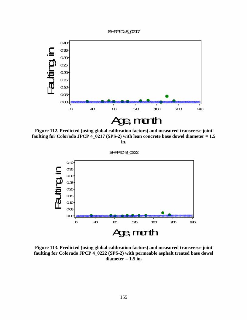
155

Figure 112. Predicted (using global calibration factors) and measured transverse joint

faulting for Colorado JPCP 4_0217 (SPS-2) with lean concrete base dowel diameter = 1.5 in.

Figure 113. Predicted (using global calibration factors) and measured transverse joint faulting for Colorado JPCP 4_0222 (SPS-2) with permeable asphalt treated base dowel

diameter = 1.5 in.

Fau

lting

, in

0.00

0.05

0.10

0.15

0.20

0.25

0.30

0.35

0.40

Age, month

0 40 80 120 160 200 240

SHRPID=8_0217

Fau

lting

, in

0.00

0.05

0.10

0.15

0.20

0.25

0.30

0.35

0.40

Age, month

0 40 80 120 160 200 240

SHRPID=8_0222

Figurfaulti

New JPC Global M Verificatthe MEPpredictedfull detaipresented

Figure

re 114. Preding for Colo

CP and Unb

MEDPG JPC

tion of the MDG analysis

d versus meails of the outd in Table 74

115. Predic

Fau

lting

, in

R2 = 81SEE = 7N = 182

dicted (usingorado JPCP

bonded JPC

P Smoothne

MEPDG globs for all selecasured IRI ustcome of stat4.

cted JPCP I

0.00

0.05

0.10

0.15

0.20

0.25

0.30

0.35

0.40

0

1 percent 7.7 in/mile 2

g global caliP 4_7776 (G

diam

CP Smoothn

ess Model V

bal JPCP IRIcted projectssing the seletistical analy

RI versus mco

A

40 8

SHR

156

ibration factGPS-3) with meter = 1.5 in

ness

erification

I model for Cs and evaluatected Coloradysis to charac

measured Cooefficients.

Age, mo

80 120

HRPID=8_7776

tors) and mdense graden.

Colorado conting goodnedo projects icterized goo

olorado JPC

month

160

measured traed aggregat

nditions conss of fit and is shown in F

odness of fit

CP with glo

200 2

ansverse joite base dow

nsisted of runbias. A plot

Figure 115,and bias are

obal calibrat

240

int el

nning t of and

e

tion

157

Table 74. Goodness of fit and bias test statistics for final Colorado calibrated JPCP IRI

model (based on 100 percent of all selected projects).

Analysis Type Diagnostic Statistics Results

Goodness of Fit R2 80.9 percent SEE 9.85 in/mi N 279

Bias H0: Slope = 1.0 p-value = 0.6458 H0: Predicted - measured IRI = 0 (paired t-test)

p-value = 0.2760

These results indicate that goodness of fit was very good, and predicted IRI exhibited no significant bias. Based on the outcome of the global model verification analysis, there was no need for local calibration. Figures 116 through 118 illustrate the global JPCP IRI model prediction for various Colorado JPCP projects over time. The predictions show a good fit of predicted and measured IRI. JPCP designs based in part on IRI in Colorado will be more accurate and optimum (lower cost) at the selected level of design reliability when done with this model.

Figure 116. Predicted and measured JPCP IRI for Colorado LTPP section 0216 over time.

IRI, in

/mi

40

80

120

160

200

Age, months

0 24 48 72 96 120 144 168 192 216 240

SHRPID=8_0216

158



Estimating Design Reliability for New JPCP and Unbonded JPCP Overlay Distress Models JPCP standard error of the estimated distress models was adopted from NCHRP 20-07(288) and are presented as follows (Mallela et al., 2011):

IRI, in

/mi

40

80

120

160

200

Age, months

0 24 48 72 96 120 144 168 192 216 240

SHRPID=8_0259

IRI, in

/mi

40

80

120

160

200

Age, months

0 24 48 72 96 120 144 168 192 216 240

SHRPID=8_7776

159

Stdev(CRK) = 1.5+(57.08*PCRK)0.33 (17) Stdev(FLT) = 0.0831*(PFLT0.3426)+0.00521 (18)

where

Stdev(CRK) = transverse fatigue crack standard deviation, percent slabs PCRK = predicted transverse fatigue cracking, percent slabs Stdev(FLT) = faulting standard deviation, in PFLT = predicted joint faulting

Smoothness IRI standard error is estimated internally by the MEPDG.

160

CHAPTER 8. INTERPRETATION OF RESULTS—DECIDING ADEQUACY OF CALIBRATION PARAMETERS Verification of Colorado MEPDG Models (Sensitivity Analysis) The researchers performed a comprehensive sensitivity study as the first step in validating the local CDOT MEPDG calibrated models. This was accomplished as follows:

Selection of an analysis period of 20 years. Development of baseline new pavement designs (HMA and JPCP) with inputs that

represent typical CDOT site conditions (climate, traffic, and subgrade), design and construction practices, and pavement materials:

o For HMA pavement, inputs included AADTT, HMA thickness, asphalt binder type, AC air voids content, AC volumetric binder content, climate, granular base thickness, and granular subbase thickness.

o For new JPCP, inputs included AADTT, base type and thickness, base erodibility index, loss of bond age at the PCC/base interface, joint spacing, PCC thickness, PCC 28-day flexural strength, shoulder type, transverse joint load transfer mechanism, PCC slab width, climate, and PCC CTE.

Key inputs were varied one at a time (except where two inputs have known correlations, such as PCC modulus of rupture and elastic modulus) across the range of typical values.

Predicted outcomes (distresses and IRI) were then plotted input by input to illustrate their impact on distress and IRI.

The impact on key performance outputs was assessed. The baseline designs are detailed in Tables 75 and 76. The range of the key inputs used for sensitivity analysis is also presented in the tables. Figures 119 through 125 present sensitivity plots for HMA pavements and JPCP distresses and smoothness (IRI). The plots shows for each key pavement input of interest the levels of distress/IRI exhibited after 20 years in service. Cumulative traffic applied over the 20-year period was 9.3 million and 9.8 million for new HMA pavements and new JPCP, respectively.

161

Table 75. Mean (baseline) and range of key inputs used for sensitivity analysis of new HMA pavements.

Input Parameter Values

Lower End Mean (Baseline) Upper End Conventional HMA thickness, in 5 in 7 in 11 Granular base thickness, in 0 in 6 in 12 in Granular subbase thickness, in 0 in 18 in 36 in Air voids, percent 3% 7% 9% Volumetric binder content, percent 7% 11% 13% Binder type (Superpave) PG 58-28 PG 64-22 PG 76-28 Initial AADTT 500 2000 5000 Cumulative trucks (after 20 years in service) Climate (weather stations)* Very cool Cool Moderate *See Table 10.

Table 76. Mean (baseline) and range of key inputs used for sensitivity analysis of new JPCP.

Input Parameter Values

Lower End Mean (Baseline) Upper End PCC Thickness, in 8-in 9-in 10-in

CTE, in/in/oF 4.5 in/in/deg. F 5 in/in/deg. F 5.5 in/in/deg. F Base type/thickness No base 4-in DGAB ATB/CTB

Dowel diameter, in (used PCC thickness/8 rule)

No dowel (0-in) 1.25-in 1.5-in

Joint spacing 12-ft 15-ft 18-ft Flexural strength, psi 600 psi 650 psi 750 psi

Shoulder type AC shoulder Tied PCC shoulder with

40% LTE Tied PCC shoulder with

70% LTE

Climate (weather stations)*

Lamar (Moderate) Approximate 7-day

highest temperature = 90.6 oF, elevation =

3,070 ft

Denver (Moderate) Approximate 7-day

highest temperature = 94.2 oF, elevation =

5,607 ft

Elbert (Very cool) Approximate 7-day

highest temperature = 79.7 oF, elevation = 7,060

ft *See Table 10.

162

Figure 119.. Sensitivity summmary for HM

craMA pavement aacking for the b

lligator crackinbaseline project

ng. Note the ret in Table 75.

ed line represennts predicted al

lligator

163

Figure 120. Sensitivity summmary for HMA

represents preA pavement totedicted rut dep

tal (HMA, granpth for the base

nular base, andeline project in

d subgrade) rutTable 75.

tting. Note the red line

164

Figure 121. SSensitivity summmary for HMAtransver

A pavement trarse cracking for

nsverse “thermr the baseline p

mal” cracking. Nproject in Table

Note the red line 75.

ne represents p

predicted

165

FFigure 122. Sennsitivity summary for HMA ppavement IRI.

Note the red linTable 75.

ne represents ppredicted IRI f

for the baseline

e project in

166

Figure 123. SSensitivity summary for JPCPcra

P transverse “sacked for the b

lab” cracking.

baseline project

Note the red lit in Table 76.

ine represents p

predicted perce

ent slabs

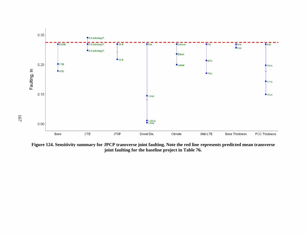
167

Figure 124. SSensitivity summmary for JPCPjoint

P transverse joifaulting for the

int faulting. Noe baseline proj

ote the red line ect in Table 76

represents pre6.

edicted mean tr

ransverse

168

Figure 125. Sensitivity summmary for JPCP IIRI. Note the r

ed line represe

ents predicted IIRI for the baseeline project in

n Table 76.

169

HMA Pavements Alligator Cracking The sensitivity results for HMA alligator cracking show HMA thickness was the most sensitive of the input variables analyzed. A change in HMA thickness from 5 to 11 inches resulted in a significant reduction in alligator cracking from approximately 90 to 0 percent lane area after 20 years in service and cumulative application of 9.3 million trucks. A similar trend was observed for full-depth HMA pavements. Base thickness, AC air void content, volumetric binder content, and the number of cumulative truck applications were the next most significant input variables, with an approximately 20 to 30 percent lane area change in alligator cracking with changes in these inputs from the lower to upper end values. Asphalt binder type, subbase thickness, and climate were the least sensitive of the inputs evaluated, showing approximately 10 percent lane area change in alligator cracking with changes in these inputs from the lower to upper end values. The sensitivity analysis trends for alligator cracking were reasonable. The magnitude of change in alligator cracking and direction of change as the input values changed were also assessed to be reasonable. The information assembled will be valuable in helping pavement design engineers optimize designs by modifying inputs as needed. Total Rutting The sensitivity results for total rutting (HMA, granular base, and subgrade) shows AADTT, HMA thickness, climate, and asphalt binder type as the most sensitive of the input variables analyzed. This implies that pavements with significant cumulative truck traffic applications over their design life (i.e., highly trafficked interstates) will experience significant levels of rutting if remedies such as thicker HMA layers and appropriate asphalt binder type are not considered in the design. The rutting sensitivity analysis results also show that HMA pavements located in hotter climate zones exhibit significantly higher levels of rutting than comparable designs in cooler climates. The HMA mix properties (percent air voids, binder content, and binder type) also had a considerable impact on rutting, although they are not the most significant. Thus, choosing and applying the right HMA mix for a given climate would help mitigate the development and progression of total rutting.

170

HMA Transverse “Thermal” Cracking The three inputs with the most impact on HMA transverse “thermal” cracking were binder type, climate, and HMA thickness. Basically, the sensitivity analysis results showed that HMA pavement located in cooler climate zones are more likely to experience significant levels of transverse cracking. Pavements with thinner HMA layers also exhibited considerably highly cracking levels than thicker HMA sections. Finally, as expected, asphalt binders with lower pavement temperature rating (-22 versus -28 °C) were more resistant to low temperature cracking. Other key HMA mix properties (binder content and air voids) had minimal impact on transverse cracking development and progression. New HMA IRI The sensitivity analysis results show that, in general, the pavement design and material properties that had a significant impact on distress development and progression (alligator cracking, rutting, transverse cracking) also affect smoothness (IRI). This is as expected, as smoothness deterioration is mostly due to distress development and future deterioration rates (severity). Key inputs that had the most significant impact on IRI included HMA air voids, binder type, AADTT, climate zone, and HMA thickness. JPCP Transverse “Slab” Cracking The sensitivity analysis results show that PCC flexural strength, PCC slab length (i.e., joint spacing), climate, PCC thickness, edge support (shoulder type and lane to shoulder load transfer efficiency), and base type had the most impact on transverse “slab” cracking development and progression. Designers can modify these inputs as needed to optimize JPCP designs. The sensitivity analysis results also show that the two site factors with the greatest impact on transverse cracking are truck traffic applications and climate (climate zone in which the pavement is located). JPCP subjected to high truck traffic applications or located in very cold climates (higher elevations) exhibited significantly higher levels of cracking. Transverse Joint Faulting Sensitivity analysis results show that the transverse joint load transfer mechanism (aggregate interlock versus dowels) and dowel diameter had the greatest impact on transverse joint faulting. Next were climate and PCC thickness. CTE, joint spacing, and edge support followed as the third group of sensitive inputs. Trends observed for all of these inputs were found to be reasonable. Designers can modify these inputs as needed to optimize JPCP designs. JPCP IRI The sensitivity analysis results show that, in general, the pavement design and material properties that had a significant impact on distress development and progression (transverse cracking and transverse joint faulting) also affected smoothness (IRI). This is as expected, as

171

smoothness deterioration is mostly due to distress development and future deterioration rates (severity). Key inputs that had the most significant impact on IRI included dowel diameter, climate, edge support, and PCC thickness. Summary of Sensitivity Analysis Results The sensitivity analysis results showed that the MEPDG design models calibrated/verified for Colorado conditions predict reasonable estimates of distress and IRI for HMA pavements and JPCP. The models also are sensitive to pavement design, materials, and site inputs, as expected. The levels of sensitivity observed were found to be reasonable, and it was determined that sensitivity was significant enough to enable pavement designers to modify inputs as needed to optimize pavement designs. A summary of the sensitivity analysis results is presented in Tables 77 and 78.

Table 77. Summary of sensitivity analysis of new HMA pavements results.

Input Parameter Distress Types and Smoothness

Alligator Cracking

Rutting Transverse Cracking

IRI

Conventional HMA thickness H H H MGranular base thickness M M L LGranular subbase thickness L L L LAir voids M M M MVolumetric binder content M M M MBinder type (Superpave) L M H MInitial AADTT M H M MClimate (weather stations) L H H MH = high, M = moderate, and L = None to low.

Table 78. Summary of sensitivity analysis of new JPCP results.

Input Parameter Distress Types and Smoothness

Transverse Cracking

Transverse Joint Faulting

IRI

PCC thickness H M M CTE M M M

Base type/thickness L M LDowel diameter, in (used PCC

thickness/8 rule) L H

M

Joint spacing H M MFlexural strength H L L

Shoulder type H H MClimate (weather stations) M M M

H = high, M = moderate, and L = None to low.

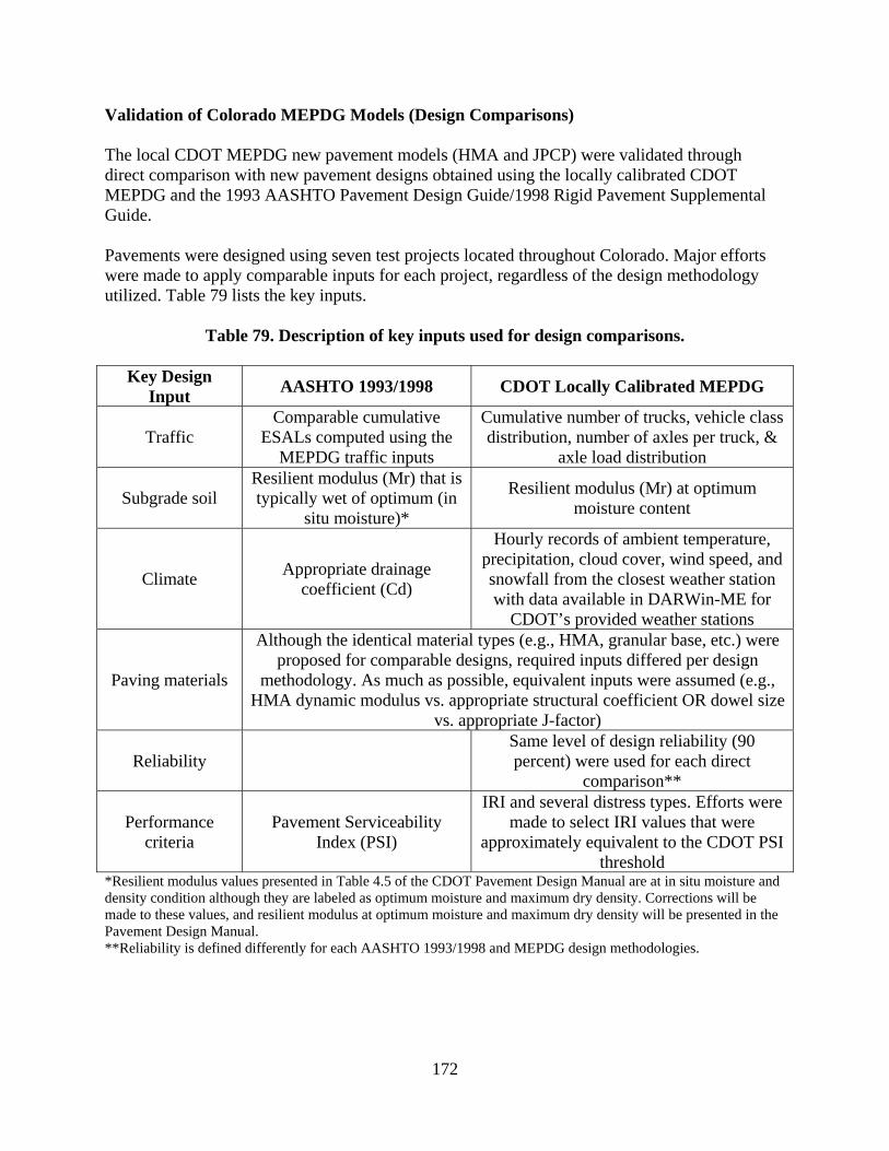
172

Validation of Colorado MEPDG Models (Design Comparisons) The local CDOT MEPDG new pavement models (HMA and JPCP) were validated through direct comparison with new pavement designs obtained using the locally calibrated CDOT MEPDG and the 1993 AASHTO Pavement Design Guide/1998 Rigid Pavement Supplemental Guide. Pavements were designed using seven test projects located throughout Colorado. Major efforts were made to apply comparable inputs for each project, regardless of the design methodology utilized. Table 79 lists the key inputs.

Table 79. Description of key inputs used for design comparisons.

Key Design Input

AASHTO 1993/1998 CDOT Locally Calibrated MEPDG

Traffic Comparable cumulative

ESALs computed using the MEPDG traffic inputs

Cumulative number of trucks, vehicle class distribution, number of axles per truck, &

axle load distribution

Subgrade soil Resilient modulus (Mr) that is typically wet of optimum (in

situ moisture)*

Resilient modulus (Mr) at optimum moisture content

Climate Appropriate drainage

coefficient (Cd)

Hourly records of ambient temperature, precipitation, cloud cover, wind speed, and snowfall from the closest weather station with data available in DARWin-ME for

CDOT’s provided weather stations

Paving materials

Although the identical material types (e.g., HMA, granular base, etc.) were proposed for comparable designs, required inputs differed per design

methodology. As much as possible, equivalent inputs were assumed (e.g., HMA dynamic modulus vs. appropriate structural coefficient OR dowel size

vs. appropriate J-factor)

Reliability Same level of design reliability (90 percent) were used for each direct

comparison**

Performance criteria

Pavement Serviceability Index (PSI)

IRI and several distress types. Efforts were made to select IRI values that were

approximately equivalent to the CDOT PSI threshold

*Resilient modulus values presented in Table 4.5 of the CDOT Pavement Design Manual are at in situ moisture and density condition although they are labeled as optimum moisture and maximum dry density. Corrections will be made to these values, and resilient modulus at optimum moisture and maximum dry density will be presented in the Pavement Design Manual. **Reliability is defined differently for each AASHTO 1993/1998 and MEPDG design methodologies.

New HM Table 80Figure 12using thepossible between procedur

I-25

Figur

MA Pavemen

shows a sum26 shows a de two design bias in desigthe AASHT

re for both re

Table 80

Proje

US 285 HamI-70 E o

Denver (ReconI-25 D

(HMA OverUS 50

(HMA OverUS 50

(PCC OverlUS 85 A

re 126. AAS

R2 = 95.3 pSEE = 0.44N = 5

nt Design Co

mmary of thdirect compamethodolog

gn HMA thicTO 1993 HMeconstruction

0. Summary

ct Site

mpden Ave. of Mack nstruction 20 y

Denver rlay 10 years) 0 East rlay 10 years) 0 East lay 30 years)

Ault/Nunn

SHTO 1993

percent 4 in

omparisons

e results fromarison of HMgies. Table 8ckness result

MA design prn and overla

of the resu

(N7

years) 1

6

HMA desigdesig

173

m the new HMA thickness81 shows thets. The resulrocedure andays.

lts from the

Traffic No. of Trucks)7.07 million 6.5 million 2.8 million

1.26 million

2.8 million

9.0 million

6.62 million

gn thicknessgn thickness

HMA designses achieved

e results of telts show veryd the AASHT

e new HMA

HMAAASHT

7.7564

4

No D

6.2

s vs. AASHTs.

ns at seven prd for all projests performy good 1-to-TO DARWi

A design pro

A Design ThicTO 1993 D75 .5 .5 .0

.0

Design

25

TO DARW

roject sites. ect comparised to identif-1 comparison-ME design

ojects.

ckness (in) DARWin-ME

8.5 6.0 7.5 4.0

4.0

No Design

6.00

Win-ME HM

sons fy on n

E

A

174

Table 81. New HMA pavement goodness of fit and bias test for final local CDOT MEPDG and 1993/1998 AASHTO Pavement Design Guide design thicknesses.

Analysis Type Diagnostic Statistics Results

Goodness of Fit R2 95.3 percent SEE 0.44 in N 5

Bias H0: Intercept = 0 p-value = 0.3684 H0: Slope = 1.0 p-value = 0.0856 H0: Predicted - measured thickness = 0 (paired t-test) p-value = 0.1576

New JPCP Design Comparisons Table 82 shows a summary of the results from the new JPCP designs at seven project sites. Figure 127 shows a direct comparison of PCC thicknesses achieved for all project comparisons. Table 83 shows the results of tests performed to identify possible bias in design PCC thickness results. The results show very good 1-to-1 comparison between the AASHTO 1998 PCC design procedure and the AASHTO DARWin-ME design procedure for both reconstruction and overlays. A direct correlation of all the PCC thickness results was shown in Figure 127. The intercept and slope of the linear curve developed using thicknesses from the two design procedures shows an approximate intercept of 0.0 and slope of 1.0, as confirmed to the 95 significance level through statistical hypothesis testing. A paired t-test of the two sets of design HMA and PCC thicknesses also indicated no significant differences. The outcomes indicate a good correlation between the CDOT MEPDG and the earlier AASHTO pavement design procedures for basic designs. Thus, the use of the CDOT MEPDG in general must yield basic designs comparable to current CDOT pavement designs. Using the superior analytical procedures of the MEPDG, however, CDOT engineers must be capable of optimizing the basic designs by selecting more appropriate materials and design inputs to produce more cost-effective pavement designs. It is noted that all of these projects are at locations that experience relative lower truck traffic. For heavier truck traffic, there may be significant differences, with the MEPDG showing slightly lower thickness than the 1993/1998 AASHTO procedure.

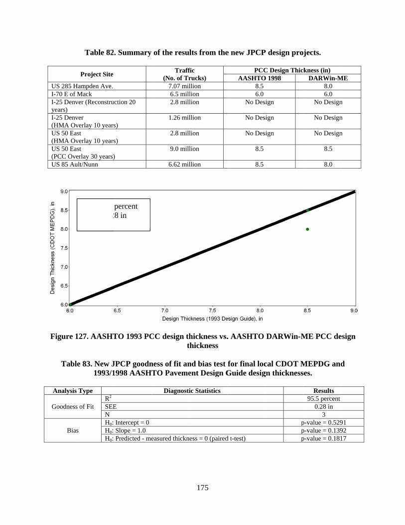
US 285 HI-70 E of I-25 Denvyears) I-25 Denv(HMA OvUS 50 Ea(HMA OvUS 50 Ea(PCC OvUS 85 Au

Figure 1

Tabl

Analysis

Goodness

Bia

Table 82

Project Site

Hampden Ave. f Mack ver (Reconstru

ver verlay 10 yearast verlay 10 yearast erlay 30 years)ult/Nunn

127. AASHT

le 83. New J1993/1

s Type

s of Fit R2 SEEN

as H0:H0:H0:

R2 = 95.5 SEE = 0.2N = 3

. Summary

uction 20

s)

s)

)

TO 1993 PC

JPCP goodn1998 AASH

E

Intercept = 0 Slope = 1.0 Predicted - me

percent 28 in

of the resu

Traff(No. of Tr

7.07 mil6.5 mill2.8 mill

1.26 mil

2.8 mill

9.0 mill

6.62 mil

CC design tht

ness of fit anTO Paveme

Diagnosti

easured thickn

175

lts from the

fic rucks) llion lion lion

llion

lion

lion

llion

hickness vs.thickness

nd bias test ent Design G

ic Statistics

ess = 0 (paired

e new JPCP

PCCAASHTO

8.56.0

No Des

No Des

No Des

8.5

8.5

. AASHTO

for final locGuide desig

d t-test)

P design pro

C Design ThicO 1998

sign

sign

sign

DARWin-M

cal CDOT Mgn thickness

ppp

ojects.

ckness (in) DARWin-M

8.0 6.0

No Design

No Design

No Design

8.5

8.0

ME PCC de

MEPDG andses.

Results 95.5 percent

0.28 in 3

p-value = 0.529p-value = 0.139p-value = 0.181

ME

n

n

n

esign

d

91 92 17

176

CHAPTER 9. SUMMARY AND CONCLUSIONS The MEPDG is based on mechanistic-empirical design concepts. This means that the design procedure calculates pavement responses such as stresses, strains, and deflections under axle loads and climatic conditions and then accumulates the damage over the design analysis period. The procedure then empirically relates calculated damage over time to pavement distresses and smoothness based on performance of actual projects. Implementing the MEPDG in Colorado has involved several major efforts to provide assurance to CDOT that the MEPDG models will predict distresses and IRI that match Colorado experience:

Development of Colorado procedures for proper inputs for using the MEPDG to design new, reconstructed, and rehabilitated pavement structures. This was accomplished through the development of a Colorado MEPDG User’s Guide that provides guidance on obtaining proper design inputs.

Verification, validation, and calibration with Colorado performance data of the MEPDG models (if necessary) to remove bias (consistent over- or under-prediction) and improve accuracy of prediction. This was accomplished through the verification, validation, and recalibration of Colorado calibration coefficients. In nearly all cases, this resulted in improved accuracy of the distress and IRI models and the removal of bias.

Design comparisons and sensitivity studies that help to establish confidence in the pavement design results achieved when using the MEPDG.

The various MEPDG prediction models have been verified, validated, and if necessary, recalibrated using Colorado LTPP and pavement management system sections. One hundred twenty-six new HMA, new JPCP, HMA/JPCP, and unbonded JPCP over JPCP rehabilitated pavements were included in a valuable database that represents the performance of Colorado pavements over many years. The model verification and calibration effort was successful and provides CDOT with validated distress and IRI models. This database was used in the verification, validation, and recalibration process to modify the prediction models to make them more accurate and unbiased (neither over- nor under-prediction). They were also used to establish Colorado design inputs and the appropriate standard deviation or error of each model for use in reliability design. This will make it possible to design a pavement in Colorado with the desired reliability at the optimum cost.

177

REFERENCES AASHTO. (1961). Interim Guide for Design of Pavement Structures. American Association of State Highway and Transportation Officials, Washington, D.C. AASHTO. (1972). Interim Guide for Design of Pavement Structures. American Association of State Highway and Transportation Officials, Washington, D.C. AASHTO. (1986). Guide for Design of Pavement Structures. American Association of State Highway and Transportation Officials, Washington, D.C. AASHTO. (1993). Guide for Design of Pavement Structures. American Association of State Highway and Transportation Officials, Washington, D.C. AASHTO. (1998). Supplement to the AASHTO Guide for Design of Pavement Structures, Part II-Rigid Pavement Design and Rigid Pavement Joint Design. American Association of State Highway and Transportation Officials, Washington, D.C. AASHTO. (2008). Mechanistic-Empirical Pavement Design Guide, Interim Edition: A Manual of Practice. American Association of State Highway and Transportation Officials, Washington, D.C. AASHTO. (2010). Guide for the Local Calibration of the Mechanistic-Empirical Pavement Design Guide. American Association of State Highway and Transportation Officials, Washington, D.C. AASHTO. (2013). AASHTOWare® Pavement ME Design™ software (formerly AASHTOWare® DARWin-ME™. American Association of State Highway and Transportation Officials, Washington, D.C. ARA. (2004). “NCHRP Guide for Mechanistic-Empirical Design of New and Rehabilitated Pavement Structures.” Final Report (Volumes 1, 2 & 3), NCHRP Project 1-37A. Applied Research Associates, Inc., Champaign, IL. FHWA/NHI. (2006). “Geotechnical Aspects of Pavements.” NHI Course No. 132040, National Highway Institute, Arlington, VA. Highway Research Board. (1962). “AASHO Road Test Report 5—Pavement Research,” Special Report 61E, Washington, D.C. Mallela, J., Titus-Glover, L., Darter, M.I., Rao, C., and Bhattacharya, B., “Recalibration of M-EPDG Rigid Pavement National Models Based on Corrected CTE Values”, Final Report #20-07/Task 288, National Cooperative Highway Research Program, Transportation Research Board of National Academics, Washington, D.C., October 2011.

178

Miller, J.S., and W.Y. Bellinger. (2003). Distress Identification Manual for the Long-Term Pavement Performance Program. Report No. FHWA-RD-03-031, Federal Highway Administration, McLean, VA. Miner, M. A. (1945). “Cumulative Damage in Fatigue,” Journal of Applied Mechanics, Vol. 12, Transactions of the American Society of Mechanical Engineers. Von Quintus, H.L., J. Mallela, R. Bonaquist, C.W. Schwartz, and R.L. Carvalho. (2012). Calibration of Rutting Models for Structural and Mix Design. NCHRP Report 719, Transportation Research Board, Washington, D.C.

A-1

APPENDIX A. NEW HMA AND NEW JPCP PERFORMANCE PREDICTION MODELS This appendix describes the MEPDG models used to predict performance. Additional information is available in several other publications (AASHTO 2008, ARA 2004). New and Reconstructed HMA Pavements Alligator Cracking Alligator cracking initiates at the bottom of the HMA layers and propagates to the surface with repeated application of heavy truck axles. Alligator cracking prediction in the MEPDG begins with the computation incrementally of HMA bottom-up fatigue damage. This is done using a grid pattern throughout the HMA layers at critical depths to determine the location within the HMA layer subjected to the highest amount of horizontal tensile strain—the mechanistic parameters used to relate applied loading to fatigue damage. An incremental damage index, DI, is calculated by dividing the actual number of axle loads by the allowable number of axle loads (note that computation of damage is based on Miner’s hypothesis) within a specific time increment and axle load interval for each axle type (Miner 1945). The cumulative damage index for each critical location is determined by summing the incremental damage over time and traffic using equation A-1 (AASHTO 2008):

TplmjHMAfTplmj N

nDIDI

,,,,

,,,, (A-1)

where n = actual number of axle load applications within a specific time period j = axle load interval m = axle load type (single, tandem, tridem, quad, or special axle configuration) l = truck type using the truck classification groups included in the MEPDG p = month T = median temperature for the five temperature intervals or quintiles used to subdivide each month, °F Nf-HMA = allowable number of axle load applications for a flexible pavement and

HMA overlays to fatigue cracking The allowable number of axle load applications needed for the incremental damage index computation is shown in equation A-2 (AASHTO 2008). 3322

11ffff k

HMAk

tfHfHMAf ECCkN (A-2)

where

Nf-HMA = allowable number of axle load applications for a flexible pavement and HMA overlays to fatigue cracking

εt = tensile strain at critical locations and calculated by the structural response

A-2

model, in/in EHMA = dynamic modulus of the HMA measured in compression, psi kf1, kf2, kf3 = global field calibration parameters (kf1 = 0.007566, kf2 = -3.9492, and kf3 =

-1.281) βf1, βf2, βf3 = local or mixture specific field calibration constants; for the global

calibration effort, these constants were set to 1.0 MC 10 (A-3)

69.084.4

bea

be

VV

VM (A-4)

Vbe = effective asphalt content by volume, percent Va = percent air voids in the HMA mixture (in situ only, not mixture design)

CH = thickness correction term as follows:

HMAH

H

e

C

49.302.111

003602.0000398.0

1

(A-5)

HHMA = total HMA thickness, in Alligator cracking is calculated from the cumulative damage over time (equation 1) using the relationship presented as equation 6 (AASHTO 2008).

))((

4*22

*11160

1BottomDILogCCCCBottom

e

CFC (A-6)

where

FCBottom = area of alligator cracking that initiates at the bottom of the HMA layers, percent of total lane area DIBottom = cumulative damage index at the bottom of the HMA layers C1,2,4 = transfer function regression constants; C4= 6,000; C1=1.00; and C2=1.00

*

2*1 2CC (A-7)

856.2*2 1748.3940874.2 HMAHC (A-8)

where HHMA = total HMA thickness, in

A-3

Transverse Cracking (Low Temperature Induced) For the MEPDG, the amount of crack propagation induced by a given thermal cooling cycle is predicted using the Paris law of crack propagation (AASHTO 2008).

nC A K (A-9)

where C = change in the crack depth due to a cooling cycle K = change in the stress intensity factor due to a cooling cycle A, n = fracture parameters for the HMA mixture Experimental results indicate that reasonable estimates of A and n can be obtained from the indirect tensile creep compliance and strength of the HMA in accordance with equations A-10 and A-11 (AASHTO 2008): nELogk mHMAttA 52.2389.410 (A-10) where

mn

118.0

(A-11)

kt = coefficient determined through global calibration for each input level (Level 1 = 5.0; Level 2 = 1.5; and Level 3 = 3.0) EHMA = HMA indirect tensile modulus, psi m = mixture tensile strength, psi m = m-value derived from the indirect tensile creep compliance curve

measured in the laboratory βt = local or mixture calibration factor Stress intensity factor, K, was incorporated in the MEPDG through the use of a simplified equation developed from theoretical finite element studies (equation A-12): 56.099.145.0 otip CK (A-12)

where tip = far-field stress from pavement response model at depth of crack tip, psi

Co = current crack length, ft The amount of transverse cracking is predicted by the MEPDG using an assumed relationship between the probability distribution of the log of the crack depth to HMA layer thickness ratio and the percent of cracking. Equation A-13 shows the expression used to determine the amount of thermal cracking (AASHTO 2008):

A-4

HMA

d

dt H

CLogNTC

1

1 (A-13)

where TC = thermal cracking, ft/mi βt1 = regression coefficient determined through global calibration (400) N[z] = standard normal distribution evaluated at [z] σd = standard deviation of the log of the depth of cracks in the pavement (0.769), in Cd = crack depth, in HHMA = thickness of HMA layers, in Rutting Rutting is caused by the plastic or permanent vertical deformation in the HMA, unbound base/subbase layers, and subgrade/foundation soil. For the MEPDG, rutting is predicted by calculating incrementally the plastic vertical strain accumulated in each pavement layer due to applied axle loading. In other words, rutting is the sum of all plastic vertical strain at the mid-depth of each pavement layer within the pavement structure, accumulated over a given analysis period. The rate of pavement layer plastic deformation could vary significantly over a given time increment since (1) the pavement layer properties (HMA and unbound aggregate material and subgrade) do change with temperature (summer versus winter months) and moisture (wet versus dry) and (2) applied traffic could also be very different. The MEPDG model for calculating total rutting is based on the universal “strain hardening” relationship developed from data obtained from repeated load permanent deformation triaxial tests of both HMA mixtures and unbound aggregate materials and subgrade soils in the laboratory. The laboratory-derived relationship was then calibrated to match field measured rut depth. For all HMA mixtures types, the MEPDG field calibrated form of the laboratory derived relationship from repeated load permanent deformation tests is shown in equation A-14: rrrrr kkk

HMArzrHMAHMApHMAp Tnkh 3322110)(1)()( (A-14)

where

p(HMA) = accumulated permanent or plastic vertical deformation in the HMA layer/sublayer, in

εp(HMA) = accumulated permanent or plastic axial strain in the HMA layer/sublayer, in/in

εr(HMA) = resilient or elastic strain calculated by the structural response model at the mid-depth of each HMA sublayer, in/in

h(HMA) = thickness of the HMA layer/sublayer, in n = number of axle load repetitions T = mix or pavement temperature, °F kz = depth confinement factor

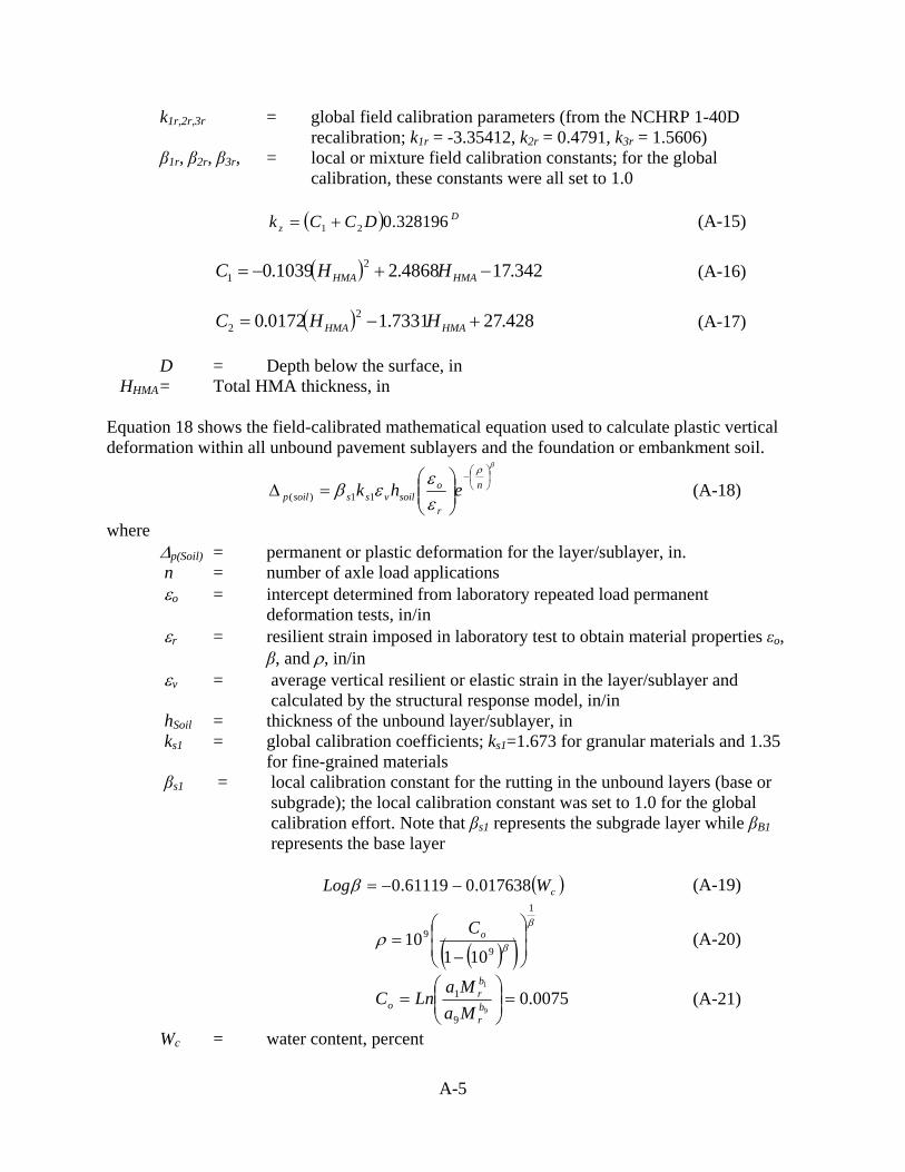
A-5

k1r,2r,3r = global field calibration parameters (from the NCHRP 1-40D recalibration; k1r = -3.35412, k2r = 0.4791, k3r = 1.5606) β1r, β2r, β3r, = local or mixture field calibration constants; for the global calibration, these constants were all set to 1.0

D

z DCCk 328196.021 (A-15)

342.174868.21039.0 21 HMAHMA HHC (A-16)

428.277331.10172.0 22 HMAHMA HHC (A-17)

D = Depth below the surface, in HHMA = Total HMA thickness, in Equation 18 shows the field-calibrated mathematical equation used to calculate plastic vertical deformation within all unbound pavement sublayers and the foundation or embankment soil.

n

r

osoilvsssoilp ehk 11)( (A-18)

where p(Soil) = permanent or plastic deformation for the layer/sublayer, in. n = number of axle load applications o = intercept determined from laboratory repeated load permanent deformation tests, in/in r = resilient strain imposed in laboratory test to obtain material properties εo, β, and , in/in v = average vertical resilient or elastic strain in the layer/sublayer and calculated by the structural response model, in/in hSoil = thickness of the unbound layer/sublayer, in ks1 = global calibration coefficients; ks1=1.673 for granular materials and 1.35

for fine-grained materials βs1 = local calibration constant for the rutting in the unbound layers (base or subgrade); the local calibration constant was set to 1.0 for the global calibration effort. Note that βs1 represents the subgrade layer while βB1 represents the base layer cWLog 017638.061119.0 (A-19)

1

9

9

10110

oC

(A-20)

0075.09

1

9

1

br

br

oMa

MaLnC (A-21)

Wc = water content, percent

A-6

Mr = resilient modulus of the unbound layer or sublayer, psi a1,9 = regression constants; a1=0.15 and a9=20.0 b1,9 = regression constants; b1=0.0 and b9=0.0 Smoothness (IRI) The design premise included in the MEPDG for predicting smoothness degradation is that the development of surface distress will result in a reduction in smoothness (increasing IRI). Equations A-22 and A-23 were developed using data from the LTPP program and are embedded in the MEPDG to predict the IRI over time for new HMA pavements (AASHTO 2008).

RDTCFCSFIRIIRI Totalo 0.400080.0400.00150.0 (A-22)

where IRIo = initial IRI after construction, in/mi SF = site factor, refer to equation A-23 FCTotal = area of fatigue cracking (combined alligator, longitudinal,

and reflection cracking in the wheel path), percent of total lane area. All load related cracks are combined on an area basis – length of cracks is multiplied by 1 foot to convert length into an area basis

TC = length of transverse cracking (including the reflection of transverse cracks in existing HMA pavements), ft/mi.

RD = average rut depth, in The site factor is calculated in accordance with the following equation: SF = FROSTH + SWELLP*AGE1.5 (A-23) where FROSTH = LN([PRECIP+1]*FINES*[FI+1]) SWELLP = LN([PRECIP+1]*CLAY*[PI+1]) FINES = FSAND + SILT AGE = pavement age, years PI = subgrade soil plasticity index PRECIP = mean annual precipitation, in. FI = mean annual freezing index, deg. F Days

FSAND = amount of fine sand particles in subgrade (percent of particles between 0.074 and 0.42 mm)

SILT = amount of silt particles in subgrade (percent of particles between 0.074 and 0.002 mm) CLAY = amount of clay size particles in subgrade (percent of particles less than 0.002 mm)

A-7

New JPCP Transverse Slab Cracking The MEPDG considers both JPCP bottom-up and top-down modes of transverse “slab” cracking. Under typical service conditions, the potential for either mode of cracking is present in all slabs. Any given slab may crack either from bottom-up or top-down, but not both. Therefore, the predicted bottom-up and top-down cracking are not particularly meaningful by themselves, and combined cracking is reported excluding the possibility of both modes of cracking occurring on the same slab. The percentage of slabs with transverse cracks (including all severities) in a given traffic lane is used as the measure of transverse cracking and is predicted using the following globally calibrated equation for both bottom-up and top-down cracking (AASHTO 2008):

05.2*6.01

1

FDI

CRK (A-24)

where

CRK = predicted amount of bottom-up or top-down cracking (fraction) DIF = fatigue damage calculated using the procedure described in this section

The general expression for fatigue damage accumulations considering all critical factors for JPCP transverse cracking is as follows (based on Miner’s hypothesis) (Miner 1945):

onmlkji

onmlkjiF N

nDI

,,,,,,

,,,,,, (A-25)

where

DIF = total fatigue damage (top-down or bottom-up) ni,j,k, ... = applied number of load applications at condition i, j, k, l, m, n Ni,j,k, … = allowable number of load applications at condition i, j, k, l, m, n i = age (accounts for change in PCC modulus of rupture and elasticity,

slab/base contact friction, traffic loads) j = month (accounts for change in base elastic modulus and effective dynamic modulus of subgrade reaction) k = axle type (single, tandem, and tridem for bottom-up cracking; short, medium, and long wheelbase for top-down cracking) l = load level (incremental load for each axle type) m = equivalent temperature difference between top and bottom PCC surfaces n = traffic offset path o = hourly truck traffic fraction

The applied number of load applications (ni,j,k,l,m,n) is the actual number of axle type k of load level l that passed through traffic path n under each condition (age, season, and temperature difference). The allowable number of load applications is the number of load cycles at which fatigue failure is expected on average and is a function of the applied stress and PCC strength.

A-8

The allowable number of load applications is determined using the following globally calibrated PCC fatigue equation:

2

,,,,,1,,,,,log

C

nmlkji

inmlkji

MRCN

(A-26)

where: Ni,j,k,… = allowable number of load applications at condition i, j, k, l, m, n. MRi = PCC modulus of rupture at age i, psi. σi,j,k, . = applied stress at condition i, j, k, l, m, n C1 = calibration constant, 2.0 C2 = calibration constant, 1.22

The fatigue damage calculation is a process of summing damage from each damage increment. Once top-down and bottom-up damage are estimated, the corresponding cracking is computed using equation A-24 and the total combined cracking determined using equation A-27. 100 downTopupBottomdownTopupBottom CRKCRKCRKCRKTCRACK (A-27)

where:

TCRACK = total transverse cracking (percent, all severities) CRKBottop-up = predicted amount of bottom-up transverse cracking (fraction) CRKTop-down = predicted amount of top-down transverse cracking (fraction)

Equation A-27 assumes that a slab may crack from either bottom-up or top-down, but not both. Transverse Joint Faulting The mean transverse joint faulting is predicted incrementally on a monthly basis. The magnitude of increment is based on current faulting level, the number of axle loads applied, pavement design features, material properties, and climatic conditions. Total faulting is determined as a sum of faulting increments from all previous months (i.e., since traffic opening) using the following equations (AASHTO 2008):

m

iim FaultFault

1

(A-28)

iiii DEFaultFAULTMAXCFault *)(* 21134 (A-29)

65

170 C *C CEROD

m

jji LogDEFAULTMAXFAULTMAX

(A-30)

6

)*

(*)0.5*1(* *C 2005curling120

C

s

EROD

P

WetDaysPLogCLogFAULTMAX

(A-31)

where

Faultm = mean joint faulting at the end of month m, in

A-9

ΔFaulti = incremental change (monthly) in mean transverse joint faulting during month i, in

FAULTMAXi = maximum mean transverse joint faulting for month i, in FAULTMAX0 = initial maximum mean transverse joint faulting, in EROD = base/subbase erodibility factor DEi = differential density of energy of subgrade deformation accumulated during month i δcurling = maximum mean monthly slab corner upward deflection PCC due to temperature curling and moisture warping PS = overburden on subgrade, lb P200 = percent subgrade material passing No. 200 sieve WetDays = average annual number of wet days (greater than 0.1 inch

rainfall) C1,2,3,4,5,6,7,12,34 = global calibration constants

Calibration Coefficients

New JPCP JPCP subjected to

CPR C1 0.5104 0.5104 C2 0.00838 0.00838 C3 0.00147 0.00147 C4 0.008345 0.008345 C5 5999 5999 C6 0.8404 0.8404 C7 5.9293 5.9293 C8 400 400

C12 and C34 are defined by equations A-32 and A-33. 25.0

2112 *C CC FR (A-32)

25.04334 *C CC FR (A-33)

FR = base freezing index defined as percentage of time the top

base temperature is below freezing (32 °F) temperature. Since the maximum faulting development occurs during nighttime when the PCC slab is curled upward and joints are opened and the load transfer efficiencies are lower, only axle load repetitions applied from 8 PM to 8 AM are considered in the faulting analysis. Smoothness (IRI) In the MEPDG, JPCP smoothness is predicted as a function of the initial as-constructed smoothness and any change in pavement longitudinal profile over time and traffic due to distress development and progression and foundation movements. The IRI model was calibrated and validated using LTPP data that represented variety of design, materials, foundations, and climatic conditions. The following is the final globally calibrated model (AASHTO 2008):

A-10

IRI = IRII + C1*CRK +C2*SPALL + C3*TFAULT + C4*SF (A-34) where

IRI = predicted IRI, in/mi IRII = initial smoothness measured as IRI, in/mi CRK = percent slabs with transverse cracks (all severities) SPALL = percentage of joints with spalling (medium and high severities) TFAULT = total joint faulting cumulated per mi, in C1 = 0.8203 C2 = 0.4417 C3 = 0.4929 C4 = 25.24 SF = site factor

SF =AGE (1+0.5556*FI) (1+P200)*10-6 (A-35)

where

AGE = pavement age, yr FI = freezing index, °F-days P200 = percent subgrade material passing No. 200 sieve

The transverse cracking and faulting are obtained using the MEPDG models described earlier. The transverse joint spalling is determined in accordance with equation A-36, which was calibrated using LTPP and other data (AASHTO 2008):

SCF)AGE*(-12005.11

100

0.01AGE

AGESPALL (A-36)

where

SPALL = percentage joints spalled (medium- and high-severities) AGE = pavement age since construction, years SCF = scaling factor based on site-, design-, and climate-related variables

SCF = –1400 + 350 • ACPCC • (0.5 + PREFORM) + 3.4 f'c • 0.4 (A-37)

– 0.2 (FTcycles • AGE) + 43 HPCC – 536 WCPCC

ACPCC = PCC air content, percent AGE = time since construction, years PREFORM = 1 if preformed sealant is present; 0 if not f'c = PCC compressive strength, psi FTcycles = average annual number of freeze-thaw cycles HPCC = PCC slab thickness, in WCPCC = PCC water/cement ratio

Documents

No. CDOT-2013-4 Final R