No-Arbitrage Taylor Rules∗

Andrew Ang†

Columbia University, USC and NBER

Sen Dong‡

Columbia University

Monika Piazzesi§

University of Chicago and NBER

This Version: 3 February 2005

JEL Classification: C13, E43, E52, G12

Keywords: affine term structure model,monetary policy, interest rate risk

∗We especially thank Bob Hodrick for providing detailed comments and valuable suggestions.We thank Ruslan Bikbov, Dave Chapman, Mike Chernov, John Cochrane, Michael Johannes, DavidMarshall, and George Tauchen for helpful discussions and we thank seminar participants at theAmerican Finance Association, Columbia University, the European Central Bank, and USC forcomments. Andrew Ang and Monika Piazzesi both acknowledge financial support from the NationalScience Foundation.

†Marshall School of Business at USC, 701 Exposition Blvd, Rm 701, Los Angeles, CA 90089-1427;ph: (213) 740-5615; fax: (213) 740-6650; email: aa610@columbia.edu; WWW: http://www.columbia.edu/∼aa610

‡Columbia Business School, 3022 Broadway 311 Uris, New York, NY 10027; email: sd2068@columbia.edu; WWW: http://www.columbia.edu/∼sd2068

§University of Chicago, Graduate School of Business, 5807 S. Woodlawn, Chicago, IL 60637;ph: (773) 834-3199; email: monika.piazzesi@gsb.uchicago.edu; WWW: http://gsbwww.uchicago.edu/fac/monika.piazzesi/research/

Abstract

We estimate Taylor (1993) rules and identify monetary policy shocks using no-arbitrage

pricing techniques. Long-term interest rates are risk-adjusted expected values of future short

rates and thus provide strong over-identifying restrictions about the policy rule used by the

Federal Reserve. The no-arbitrage framework also accommodates backward-looking and

forward-looking Taylor rules. We find that inflation and GDP growth account for over half

of the time-variation of yield levels and we attribute almost all of the movements in the term

spread to inflation. Taylor rules estimated with no-arbitrage restrictions differ substantially

from Taylor rules estimated by OLS and monetary policy shocks identified with no-arbitrage

techniques are less volatile than their OLS counterparts.

1 Introduction

Most central banks, including the U.S. Federal Reserve (Fed), conduct monetary policy to only

influence the short end of the yield curve. However, the entire yield curve responds to the

actions of the Fed because long interest rates are conditional expected values of future short

rates, after adjusting for risk premia. These risk-adjusted expectations of long yields are formed

based on a view of how the Fed conducts monetary policy using short yields. Thus, the whole

yield curve reflects the monetary actions of the Fed, so the entire term structure of interest rates

can be used to estimate monetary policy rules and extract estimates of monetary policy shocks.

According to the Taylor (1993) rule, the Fed sets short interest rates by reacting to

CPI inflation and the deviation of GDP from its trend. To exploit the over-identifying no-

arbitrage movements of the yield curve, we place the Taylor rule in a term structure model

that excludes arbitrage opportunities. The assumption of no arbitrage is reasonable in a world

of large investment banks and active hedge funds, who take positions eliminating arbitrage

opportunities arising in bond prices that are inconsistent with each other in either the cross-

section or their expected movements over time. Moreover, the absence of arbitrage is a

necessary condition for standard equilibrium models. Imposing no arbitrage therefore can

be viewed as a useful first step towards a structural model.

We describe expectations of future short rates by the Taylor rule and a Vector Autoregres-

sion (VAR) for macroeconomic variables. Following the approach taken in many papers in

macroeconomics (see, for example, Fuhrer and Moore, 1995; Cogley, 2003), we could infer

the values of long yields from these expectations by imposing the Expectations Hypothesis

(EH). However, there is strong empirical evidence against the EH (see, for example, Fama

and Bliss, 1987; Campbell and Shiller, 1991; Bansal, Tauchen and Zhou, 2004; Cochrane and

Piazzesi, 2004, among many others). Term structure models can account for deviations from

the EH by explicitly incorporating time-varying risk premia (see, for example, Fisher, 1998;

Dai and Singleton, 2002).

We develop a methodology to embed Taylor rules in an affine term structure model with

time-varying risk premia. The structure accommodates standard Taylor rules, backward-

looking Taylor rules that allow multiple lags of inflation and GDP growth to influence the

actions of the Fed, and forward-looking Taylor rules where the Fed responds to anticipated

inflation and GDP growth. The model specifies standard VAR dynamics for the macro

indicators, inflation and GDP growth, together with an additional latent factor that drives

interest rates and is related to monetary policy shocks. Our framework also allows risk premia

to depend on the state of the macroeconomy.

1

By combining no-arbitrage pricing with the Fed’s policy rule, we extract information from

the entire term structure about monetary policy, and vice versa, use our knowledge about

monetary policy to model the term structure of interest rates. In particular, we use information

from the whole yield curve to obtain more efficient estimates of how monetary policy shocks

affect the future path of macro aggregates. The term structure model also allows us to measure

how a yield of any maturity responds to monetary policy or macro shocks. Interestingly, the

model implies that a large amount of interest rate volatility is explained by movements in macro

variables. For example, 65% of the variance of the 1-quarter yield and 61% of the variance of

the 5-year yield can be attributed to movements in inflation and GDP growth. Over 95% of

the variance in the 5-year term spread is due to time-varying inflation and inflation risk. The

estimated model also captures the counter-cyclical properties of time-varying expected excess

returns on bonds.

To estimate the model, we use Bayesian techniques that allow us to estimate flexible

dynamics and extract estimates of latent monetary policy shocks. Existing papers that

incorporate macro variables into term structure models make strong – and often arbitrary –

restrictions on the VAR dynamics, risk premia, and measurement errors. For example, Ang

and Piazzesi (2003) assume that macro dynamics do not depend on interest rates. Dewachter

and Lyrio (2004), and Rudebusch and Wu (2004), among others, set arbitrary risk premia

parameters to be zero. Hordahl, Tristani and Vestin (2003), Rudebusch and Wu (2003), and

Ang, Piazzesi, and Wei (2004), among others, assume that only certain yields are measured

with error, while others are observed without error. These restrictions are not motivated from

economic theory, but are only made for reasons of econometric tractability. In contrast, we do

not impose these restrictions and find that the added flexibility helps the performance of the

model.

Our paper is related to a growing literature on linking the dynamics of the term structure

with macro factors. Piazzesi (2005) develops a term structure model where the Fed targets the

short rate and reacts to information contained in the yield curve. Piazzesi uses data measured

at high-frequencies to identify monetary policy shocks. By assuming that the Fed reacts to

information available right before its policy decision, she identifies the unexpected change in

the target as the monetary policy shock and identifies the expected target as the policy rule. In

contrast, we estimate Taylor rules following the large macro literature that uses the standard

low frequencies (we use quarterly data) at which GDP and inflation are reported. At low

frequencies, the Piazzesi identification scheme does not make sense because we would have to

assume that the Fed uses only lagged one-quarter bond market information and ignores more

recent data.

2

In contrast, we assume that the Fed follows the Taylor rule, and thus reacts to contem-

poraneous output and inflation numbers. This identification strategy relies on the reasonable

assumption that these macroeconomic variables react only slowly – not within the same quarter

– to monetary policy shocks. This popular identification strategy has also been used by

Christiano, Eichenbaum, and Evans (1996), Evans and Marshall (1998, 2001), and many

others. By using this strategy, we are not implicitly assuming that the Fed completely ignores

current and lagged information from the bond market (or other financial markets). To the

contrary, yields in our model depend on the current values of output and inflation. Thus, we

are implicitly assuming that the Fed cares about yield data because yields provide information

about the future expectations of macro variables.

The other papers in this literature are less interested in estimating various Taylor rules,

rather than embedding a particular form of a Taylor rule, sometimes pre-estimated, in a

macroeconomic model. For example, Bekaert, Cho, and Moreno (2003), Hordahl, Tristani,

and Vestin (2003), and Rudebusch and Wu (2003) estimate structural term structure models

with macroeconomic variables. In contrast to these studies, we do not impose any structure

in addition to the assumption of no arbitrage, which makes our approach more closely related

to the identified VAR literature in macroeconomics (for a survey, see Christiano, Eichenbaum

and Evans, 1999). This gives us additional flexibility in matching the dynamics of the term

structure. While Bagliano and Favero (1998) and Evans and Marshall (1998, 2001), among

others, estimate VARs with many yields and macroeconomic variables, they do not impose

no-arbitrage restrictions. Bernanke, Boivin and Eliasz (2004), and Diebold, Rudebusch, and

Aruoba (2004) estimate latent factor models with macro variables, but they also do not preclude

no-arbitrage movements of bond yields. Dai and Philippon (2004) examine the effect of fiscal

shocks on yields with a term structure model, whereas our focus is embedding monetary policy

rules into a no-arbitrage model.

We do not claim that our new no-arbitrage identification techniques are superior to

estimating monetary policy rules using structural models (see, among others, Bernanke and

Mihov, 1998) or using real-time information sets like central bank forecasts to control for

the endogenous effects of monetary policy taken in response to current economic conditions

(see, for example, Romer and Romer, 2004). Rather, we believe that identifying monetary

policy shocks using no-arbitrage restrictions are a useful addition to existing methods. Our

framework enables the entire cross-section and time-series of yields to be modeled and provides

a unifying framework to jointly estimate standard, backward-, and forward-looking Taylor rules

in a single, consistent framework. Naturally, our methodology can be used in more structural

approaches that effectively constrain the factor dynamics and risk premia and we can extend

3

our set of instruments to include richer information sets. We intentionally focus on the most

parsimonious set-up where Taylor rules can be identified in a no-arbitrage model.

The rest of the paper is organized as follows. Section 2 outlines the model and develops

the methodology showing how Taylor rules can be identified with no-arbitrage conditions. We

briefly discuss the estimation strategy in Section 3. In Section 4, we lay out the empirical

results. After describing the parameter estimates, we attribute the time-variation of yields and

expected excess holding period returns of long-term bonds to economic sources. We describe in

detail the implied Taylor rule estimates from the model and contrast them with OLS estimates.

We compare the no-arbitrage monetary policy shocks and impulse response functions with

traditional VAR and other identification approaches. Section 5 concludes.

2 The Model

We detail the set-up of the model in Section 2.1. Section 2.2 shows how the model implies

closed-form solutions for bond prices (yields) and expected returns. In Sections 2.3 to 2.7,

we detail how Taylor rules can be identified using the over-identifying restrictions imposed on

bond prices through no-arbitrage.

2.1 General Set-up

We denote the3× 1 vector of state variables as

Xt = [gt πt fut ]> ,

wheregt is quarterly GDP growth fromt−1 to t, πt is the quarterly inflation rate fromt−1 to t,

andfut is a latent term structure state variable. Both GDP growth and inflation are continuously

compounded. We use one latent state variable because this is the most parsimonious set-up

where the Taylor rule residuals can be identified (as the next section makes clear) using no-

arbitrage restrictions. The latent factor,fut , is a standard latent term structure factor in the

tradition of the affine term structure literature. However, we show below that this factor can be

interpreted as a transformation of policy actions taken by the Fed on the short rate.

We specify thatXt follows a VAR(1):

Xt = µ + ΦXt−1 + Σεt, (1)

whereεt ∼ IID N(0, I). The short rate is given by:

rt = δ0 + δ>1 Xt, (2)

4

for δ0 a scalar andδ1 a 3 × 1 vector. To complete the model, we specify the pricing kernel to

take the standard form:

mt+1 = exp

(−rt − 1

2λ>t λt − λtεt+1

), (3)

with the time-varying prices of risk:

λt = λ0 + λ1Xt, (4)

for the 3 × 1 vectorλ0 and the3 × 3 matrix λ1. The pricing kernel prices all assets in the

economy, which are zero-coupon bonds, from the recursive relation:

P(n)t = Et[mt+1P

(n−1)t+1 ],

whereP(n)t is the price of a zero-coupon bond of maturityn quarters at timet.

Equivalently, we can solve the price of a zero-coupon bond as

P(n)t = EQ

t

[exp

(−

n−1∑i=0

rt+i

)],

whereEQt denotes the expectation under the risk-neutral probability measure, under which

the dynamics of the state vectorXt are characterized by the risk-neutral constant and

autocorrelation matrix

µQ = µ− Σλ0

ΦQ = Φ− Σλ1.

If investors are risk-neutral,λ0 = 0 andλ1 = 0, and no risk adjustment is necessary.

This model belongs to the Duffie and Kan (1996) affine class of term structure models, but

uses both latent and observable macro factors. The affine prices of risk specification in equation

(4) has been used by, among others, Constantinides (1992), Fisher (1998), Dai and Singleton

(2002), Brandt and Chapman (2003), and Duffee (2002) in continuous time and by Ang and

Piazzesi (2003), Ang, Piazzesi and Wei (2004), and Dai and Philippon (2004) in discrete time.

As Dai and Singleton (2002) demonstrate, the flexible affine price of risk specification is able

to capture patterns of expected holding period returns on bonds that we observe in the data.

2.2 Bond Prices and Expected Returns

Ang and Piazzesi (2003) show that the model in equations (1) to (4) implies that bond yields

take the form:

y(n)t = an + b>n Xt, (5)

5

wherey(n)t is the yield on ann-period zero coupon bond at timet that is implied by the model,

which satisfiesP (n)t = exp(−ny

(n)t ).

The scalaran and the3 × 1 vectorbn are given byan = −An/n andbn = −Bn/n, where

An andBn satisfy the recursive relations:

An+1 = An + B>n (µ− Σλ0) +

1

2B>

n ΣΣ>Bn − δ0

B>n+1 = B>

n (Φ− Σλ1)− δ>1 , (6)

whereA1 = −δ0 andB1 = −δ1. In terms of notation, the one-period yieldy(1)t is the same as

the short ratert in equation (2).

Since yields take an affine form, expected holding period returns on bonds are also affine

in the state variablesXt. We define the one-period excess holding period return as:

rx(n)t+1 = log

(P

(n−1)t+1

P(n)t

)− rt

= ny(n)t − (n− 1)y

(n−1)t+1 − rt. (7)

The conditional expected excess holding period return can be computed using:

Et[rx(n)t+1] = −1

2B>

n−1ΣΣ>Bn−1 + B>n−1Σλ0 + B>

n−1Σλ1Xt

= Axn + Bx>

n Xt (8)

From this expression, we can see directly that the expected excess return comprises three

terms: (i) a Jensen’s inequality term, (ii) a constant risk premium, and (iii) a time-varying

risk premium. The time variation is governed by the parameters in the matrixλ1. Since both

bond yields and the expected holding period returns of bonds are affine functions ofXt, we

can also easily compute variance decompositions following standard methods for a VAR.

2.3 The Benchmark Taylor Rule

The Taylor (1993) rule is a convenient reduced-form policy rule that captures the notion that the

Fed adjusts short-term interest rates in response to movements in inflation and real activity. The

Taylor rule is consistent with a monetary authority minimizing a loss function over inflation

and output (see, for example, Svenson 1997). We can interpret the short rate equation (2)

of the term structure model as a Taylor rule of monetary policy. Following Taylor’s original

specification, we define the benchmark Taylor rule to be:

rt = δ0 + δ1,ggt + δ1,ππt + εMP,Tt , (9)

6

where the short rate is set by the Federal Reserve to be a function of current output and inflation.

The basic Taylor rule (9) can be interpreted as the short rate equation (2) in a standard affine

term structure model, where the unobserved monetary policy shockεMP,Tt corresponds to a

latent term structure factor,εMP,Tt = δfufu

t . This corresponds to the short rate equation (2) in

the term structure model withδ1 = (δ1,g δ1,π δ1,fu)>.

The Taylor rule (9) can be estimated consistently using OLS under the assumption that

εMP,Tt , or fu

t , is contemporaneously uncorrelated with GDP growth and inflation. If monetary

policy is effective, policy actions by the Federal Reserve today predict the future path of GDP

and inflation, causing an unconditional correlation between monetary policy actions and macro

factors. In this case, running OLS on equation (9) may not provide efficient estimates of the

Taylor rule. In our setting, we allowεMP,Tt to be unconditionally correlated with GDP or

inflation and thus our estimates should be more efficient, under the null of no-arbitrage, than

OLS. In our model, the coefficientsδ1,g andδ1,π in equation (9) are simply the coefficients on

gt andπt in the vectorδ1 in the short rate equation (2).

There are several advantages to estimating the policy coefficients,δ1, and extracting the

monetary policy shock,εMP,Tt , using no-arbitrage identification restrictions rather than simply

running OLS on equation (9). First, although OLS is consistent under the assumption that

GDP growth and inflation are contemporaneously uncorrelated withεMP,Tt , it is not efficient.

No-arbitrage allows for many additional yields to be employed in estimating the Taylor rule.

Second, the term structure model can identify the effect of a policy or macro shock on any

segment of the yield curve, which an OLS estimation of equation (9) cannot provide. Finally,

we can trace the predictability of risk premia in bond yields to macroeconomic or monetary

policy sources only by imposing no-arbitrage constraints.

The Taylor rule in equation (9) does not depend on the past level of the short rate. Therefore,

empirical studies typically find that the implied monetary policy shocks from the benchmark

Taylor rule,εMP,Tt , are highly persistent (see Rudebusch and Svensson, 1999). The reason is

that the short rate is highly autocorrelated and its movements are not well explained by the

right-hand side variables in equation (9). This causes the implied shock to inherit the dynamics

of the level of the persistent short rate. In affine term structure models, this finding is reflected

by the properties of the implied latent variables. In particular,εMP,Tt corresponds toδ1,fufu

t ,

which is the scaled latent term structure variable. Ang and Piazzesi (2003) show that the first

latent factor implied by an affine model with both latent factors and observable macro factors

closely corresponds to the traditional first, highly persistent, latent factor in term structure

models with only unobservable factors. This latent variable also corresponds closely to the

first principal component of yields, or the average level of the yield curve, which is highly

7

autocorrelated.

2.4 Backward-Looking Taylor Rules

Eichenbaum and Evans (1995), Christiano, Eichenbaum, and Evans (1996), Clarida, Gali, and

Gertler (1998), among others, consider modified Taylor rules that include current as well as

lagged values of macro variables and the previous short rate:

rt = δ0 + δ1,ggt + δ1,ππt + δ2,ggt−1 + δ2,ππt−1 + δ2,rrt−1 + εMP,Bt , (10)

whereεMP,Bt is the implied monetary policy shock from the backward-looking Taylor rule. This

formulation has the statistical advantage that we compute monetary policy shocks recognizing

that the short rate is a highly persistent process. The economic mechanism behind equation

(10) may be that the objective of the central bank is to smooth interest rates (see Goodfriend,

1991) and thus we should consider computing monetary policy shocks taking into account

lagged short rates.

In the setting of our model, we can modify the short rate equation (2) to take the same form

as equation (10). Collecting the macro factorsgt andπt into a vector of observable variables

f ot = (gt πt)

>, we can rewrite the short rate dynamics in equation (2) as:

rt = δ0 + δ>1,ofot + δ1,fufu

t , (11)

where we decompose the vectorδ1 into δ1 = (δ>1,o δ1,fu)> = (δ1,g δ1,π δ1,fu)>. We also rewrite

the dynamics ofXt = (f o>t fu

t )> in equation (1) as:(

f ot

fut

)=

(µ1

µ2

)+

(Φ11 Φ12

Φ21 Φ22

)(f o

t−1

fut−1

)+

(u1

t

u2t

), (12)

whereut = (u1>t u2

t )> ∼ IID N(0, ΣΣ>). Equation (12) is equivalent to equation (1), but the

notation in equation (12) separates the dynamics of the macro variables,f ot , from the dynamics

of the latent factor,fut .

Using equation (12), we can substitute forfut in equation (11) to obtain:

rt = (1− Φ22)δ0 + δ1,fuµ2 + δ>1,ofot + (δ1,fuΦ>

21 − Φ22δ11)>f o

t−1 + Φ22rt−1 + εMP,Bt , (13)

where we substitute for the dynamics offut in the first line and where we define the backward-

looking monetary policy shock to beεMP,Bt ≡ δ1,fuu2

t in the second line. Equation (13)

expresses the short rate as a function of current and lagged macro factors,f ot andf o

t−1, the

lagged short rate,rt−1, and a monetary policy shockεMP,Bt .

8

In equation (13), the response of the Fed to contemporaneous GDP and inflation captured

by theδ1,o coefficient onf ot is identical to the response of the Fed in the benchmark Taylor rule

(9) because theδ1,o coefficient is unchanged. The intuition behind this result is that the short

rate equation (2) already embeds the full response of the short rate to current macro factors.

The latent factor, however, represents the action of past short rates and past macro factors. We

have rewritten the benchmark Taylor rule to equivalently represent the predictable component

of the latent factor as lagged macro variables and lagged short rates. Importantly, the backward-

looking Taylor rule in equation (13) and the benchmark Taylor rule (9) are equivalent – they

are merely different ways of expressing the same relationship between yields and macro factors

captured by the term structure model.

The implied monetary policy shocks from the backwards-looking Taylor rule,εMP,Bt , are

potentially very different from the benchmark Taylor rule shocks,εMP,Tt . In the no-arbitrage

model, the backward-looking monetary policy shockεMP,Bt is identified as the scaled shock

to the latent term structure factor,δ1,fuu2t . In the set-up of the factor dynamics in equation

(1) (or equivalently equation (12)), theu2t shocks are IID. In comparison, the shocks in the

standard Taylor rule (9),εMP,Tt are highly autocorrelated. Note that the coefficients on lagged

macro variables in the extended Taylor rule (13) are equal to zero only ifδ12Φ′21 = Φ22δ1,o.

Under this restriction, the combined movements of the past macro factors must exactly offset

the movements in the lagged term structure latent factor so that the short rate is affected only

by unpredictable shocks.

Once our model is estimated, we can easily back out the implied extended Taylor rule (10)

from the estimated coefficients. This is done by using the implied dynamics offut in the factor

dynamics (12):

u2t = fu

t − µ2 − Φ21fot−1 − Φ22f

ut−1.

Again, if εMP,Bt = δ1,fuu2

t is unconditionally correlated with the shocks to the macro factors

f ot , then OLS does not provide efficient estimates of the monetary policy rule, and may provide

biased estimates of the Taylor rule in small samples.

2.5 Forward-Looking Taylor Rules

Finite Horizon Forward-Looking Taylor Rules

Clarida and Gertler (1997) and Clarida, Galı and Gertler (2000), among others, propose a

forward-looking Taylor rule, where the Fed sets interest rates based on expected future GDP

growth and expected future inflation over the next few quarters. For example, a forward-

9

looking Taylor rule using expected GDP growth and inflation over the next quarter takes the

form:

rt = δ0 + δ1,gEt(gt+1) + δ1,πEt(πt+1) + εMP,Ft , (14)

where we defineεMP,Ft to be the forward-looking Taylor rule monetary policy shock. We now

show howεMP,Ft can be identified using no-arbitrage restrictions from a term structure model.

We can compute the conditional expectation of GDP growth and inflation from our model

by noting that:

Et(Xt+1) = µ + ΦXt,

from the dynamics ofXt in equation (1). Since the conditional expectations of future GDP

growth and inflation are simply a function of currentXt, we can map the forward-looking

Taylor rule (14) into the framework of an affine term structure model. Denotingei as a vector

of zeros with a one in theith position, we can write equation (14) as:

rt = δ0 + (δ1,ge1 + δ1,πe2)>µ + (δ1,ge1 + δ1,πe2)

>ΦXt + εMP,Ft , (15)

asgt andπt are ordered as the first and second elements inXt.

Equation (15) is an affine short rate equation where the short rate coefficients are a function

of the parameters of the dynamics ofXt:

rt = δ0 + δ>1 Xt, (16)

where

δ0 = δ0 + (e1 + e2)>µ

δ1 = (δ1,ge1 + δ1,πe2)>Φ + δ1,fue3,

andεMP,Ft ≡ δ1,fufu

t . Hence, we can identify a forward-looking Taylor rule by imposing no-

arbitrage restrictions by redefining the bond price recursions in equation (6) using the newδ0

and δ1 coefficients in place ofδ0 andδ1. Hence, a complete term structure model is defined

by the same set-up as equations (1) to (4), except we use the new short rate equation (16)

that embodies the forward-looking structure, in place of the basic short rate equation (2). The

restrictions onδ0, δ1, µ, andΦ in equation (16) imply that the forward-looking Taylor rule is

effectively a constrained estimation of a general affine term structure model.

The new no-arbitrage bond recursions usingδ0 and δ1 reflect the conditional expectations

of GDP and inflation that enter in the short rate equation (16). Furthermore, the conditional

expectationsEt(gt+1) andEt(πt+1) are those implied by the underlying dynamics ofgt andπt

in the VAR process (1). Other approaches, like Rudebusch and Wu (2003), specify the future

10

expectations of macro variables entering the short rate equation in a manner not necessarily

consistent with the underlying dynamics of the macro variables. The monetary policy shocks

in the forward-looking Taylor rule (14) or (15),εMP,Ft , can be consistently estimated by OLS

only if fut is orthogonal to the dynamics ofgt andπt.

Sincek-period ahead conditional expectations of GDP and inflation remain affine functions

of the current state variablesXt, we can also specify a more general forward-looking Taylor

rule based on expected GDP or inflation over the nextk quarters:

rt = δ0 + δ1,gEt(gt+k,k) + δ1,πEt(πt+k,k) + εMP,Ft , (17)

wheregt+k,k andπt+k,k represent GDP growth and inflation over the nextk periods:

gt+k,k =1

k

k∑i=1

gt+i and πt+k,k =1

k

k∑i=1

πt+i. (18)

The forward-looking Taylor rule monetary policy shockεMP,Ft is the scaled latent term

structure factor,εMP,Ft = δ1,fufu

t . As Clarida, Galı and Gertler (2000) note, the general case

(17) also nests the benchmark Taylor rule (9) as a special case by settingk = 0. In Appendix

A, we detail the appropriate transformations required to map equation (17) into an affine term

structure model and discuss the estimation procedure for a forward-looking Taylor rule for a

k-quarter horizon.

Infinite Horizon Forward-Looking Taylor Rules

An alternative approach to assigning ak-period horizon for which the Fed considers future

GDP growth and inflation in its policy rule is that the Fed discounts the entire expected path of

future economic conditions. For simplicity, we assume the Fed discounts both expected future

GDP growth and expected future inflation at the same discount rate,β. In this formulation, the

forward-looking Taylor rule takes the form:

rt = δ0 + δ1,ggt + δ1,ππt + δ1,fufut (19)

wheregt and πt are infinite sums of expected future GDP growth and inflation, respectively,

both discounted at rateβ per period. Many papers have setβ at one, or very close to one,

sometimes motivated by calibrating it to an average real interest rate (see Salemi, 1995;

Rudebusch and Svenson, 1999; Favero and Rovelli, 2003; Collins and Siklos, 2004).

We can estimate the discount rateβ as part of a standard term structure model by using the

11

dynamics ofXt in equation (1) to writegt as:

gt =∞∑i=0

βie>1 Et(Xt+i)

= e>1 (Xt + βµ + βΦXt + β2(I + Φ)µ + β2Φ2Xt + · · · )= e>1 (µβ + (I + Φ)µβ2 + · · · ) + e>1 (I + Φβ + Φ2β2 + · · · )Xt

=β

(1− β)e>1 (I − Φβ)−1µ + e>1 (I − Φβ)−1Xt, (20)

wheree1 is a vector or zeros with a one in the first position to pick outgt, which is ordered first

in Xt. We can also write discounted future inflation,πt, in a similar fashion:

πt =β

(1− β)e>2 (I − Φβ)−1µ + e>2 (I − Φβ)−1Xt, (21)

wheree2 is a vector of zeros with a one in the second position.

In a similar fashion to mapping the Clarida-Gali-Gertler forward-looking Taylor without

discounting into a term structure model, we can accommodate a forward-looking Taylor rule

with discounting by re-writing the short rate equation (2) as:

rt = δ0 + δ>1 Xt, (22)

where

δ0 = δ0 + [δ1,ge1 δ1,πe2]>

(β

(1− β)(I − Φβ)−1µ

),

δ1 = [δ1,ge1 δ1,πe2]>(I − Φβ)−1 + δ1,fu e3. (23)

Similarly, we modify the bond price recursions for the standard affine model in equation (6) by

usingδ0 andδ1 in place ofδ0 andδ1.

2.6 Forward- and Backward-Looking Taylor Rules

As a final case, we combine the forward- and backward-looking Taylor rules, so that the

monetary policy rule is computed taking into account forward-looking expectations of macro

variables, lagged realizations of macro variables, while also controlling for lagged short rates.

We illustrate the rule considering expectations for inflation and GDP over the next quarter

(k = 1), but similar rules apply for other horizons.

We start with the standard forward-looking Taylor rule in equation (14):

rt = δ0 + δ>1,oEt(fot+1) + εMP,F

t ,

12

whereEt(fot+1) = (Et(gt+1) Et(πt+1))

> and εMP,Ft = δ1,fufu

t . We substitute forfut using

equation (12) to obtain:

rt = (1−Φ22)δ0+δ1,fuµ2+δ>1,oEt(fot+1)+(δ1,fuΦ>

21−Φ22δ1,o)>f o

t−1+Φ22rt−1+εMP,FBt , (24)

where εMP,FBt = δ1,fuu2

t is the forward- and backward-looking monetary policy shock.

Equation (24) expresses the short rate as a function of both expected future macro factors and

lagged macro factors, the lagged short rate,rt−1, and a monetary policy shock,εMP,FBt . The

forward- and backward-looking Taylor rule (24) is an equivalent representation of the forward-

looking Taylor rule in (14). Hence, similar to how the coefficients on contemporaneous macro

variables in the backward-looking Taylor rule (13) are identical to the coefficients in the

benchmark Taylor rule (9), the coefficientsδ1,o on future expected macro variables are exactly

the same as the coefficients in the forward-looking Taylor rule (14).

2.7 Summary of Taylor Rules

The no-arbitrage framework is able to estimate several structural Taylor rule specifications

from the same reduced-form term structure model. Table 1 summarizes the various Taylor

Rule specifications that can be identified by no-arbitrage restrictions. The benchmark and

backward-looking Taylor rules are different structural rules that give rise to the same reduced-

form term structure model. Similarly, the forward-looking and the backward- and forward-

looking Taylor rules produce observationally equivalent term structure models. In all cases, the

monetary policy shocks are transformations of either levels or innovations of the latent term

structure variable. Finally, the last column of Table 1 reports if the no-arbitrage model requires

additional restrictions. Both the forward-looking specifications require parameter restrictions

in the short rate equation to ensure that we compute the expectations of the macro variables

consistent with the dynamics of the VAR.

3 Data and Econometric Methodology

The objective of this section is to briefly discuss the data and the econometric methodology

used to estimate the model. In particular, we motivate our estimation approach and discuss

several econometric issues. We relegate all technical issues to Appendix C.

13

3.1 Data

To estimate the model, we use continuously compounded yields of maturities 1, 4, 8, 12, 16,

and 20 quarters, at a quarterly frequency. The bond yields of one year maturity and longer are

from the CRSP Fama-Bliss discount bond files, while the short rate (one-quarter maturity) is

taken from the CRSP Fama risk-free rate file. The sample period is June 1952 to December

2002. The consumer price index and real GDP numbers are taken from the Federal Reserve

Database (FRED) at Saint Louis.

3.2 Estimation Method

We estimate the term structure model using Markov Chain Monte Carlo (MCMC) and Gibbs

sampling methods. There are three main reasons why we choose to use a Bayesian estimation

approach. First, the term structure factor,fut , and the corresponding monetary policy shocks

implied byfut are unobserved variables. In a Bayesian estimation strategy, we obtain a posterior

distribution of the time-series path offut and monetary policy shocks. That is, the Bayesian

algorithm provides a way to compute the mean of the posterior distribution of the time-series of

fut through the sample, and, consequently, we can obtain a best estimate of implied monetary

policy shocks.

The second advantage of our estimation method is that, although the maximum likelihood

function of the model can be written down (see Ang and Piazzesi, 2003), the model is high

dimensional and extremely non-linear. This causes the maximum likelihood function to have

many possible local optima, some of which may lie in unreasonable or implausible regions

of the parameter space. In our Bayesian setting, using uninformative priors on reasonable

regions of the parameter space effectively rules out parameter values that are implausible.

A maximum likelihood estimator also involves a difficult optimization problem, whereas the

Bayesian algorithm is based on a series of simulations that are computationally much more

tractable.

Third, in a situation with only one yield and one latent factor, the maximum likelihood

function has a point mass at zero for the set of parameter values that assigns a one-to-one

correspondence between the observed yield and the latent factor. In this set of parameter values,

there is no effect of macro variables on the dynamics of interest rates and the yield is driven

entirely by the latent factor that takes on the same dynamics as the yield itself. Specifically,

in the maximum likelihood function, the coefficientsδ1,o on the observable macro variables in

equation (11) may tend to go to zero, and the feedback coefficients between the latent factor and

14

the macro variables in the VAR equation (1) may also tend to go to zero. A similar problem

occurs in our setting with a cross-section of yields and one latent factor, where a maximum

likelihood estimator may assign almost all the explanatory power to the latent factor that is

inverted from a single yield and thus gives little role to the macro factors. Given that there

must be some underlying economic relation between bond prices and macro variables, we

have strong priors that this set of parameters is not a reasonable representation of the true

joint dynamics of yields and macro variables. A Bayesian estimation avoids this stochastic

singularity by a suitable choice of priors on the Taylor rule coefficients and on the companion

form of the VAR, while avoiding the use of a single yield to identify the latent factor.

An affine term structure model can only exactly price the same number of yields as the

number of latent factors. In our case, the model in equations (1)-(4) can only price one yield

exactly since we use only one latent factor,fu. The usual estimation approach, following Chen

and Scott (1993), is to specify some (arbitrary) yield maturities to be observed without error,

and the remaining yields to have observation, or measurement, error. We do not arbitrarily

impose observation error across certain yields. Instead, we assign an observation error to each

yield, so that the equation for each yield is:

y(n)t = y

(n)t + η

(n)t , (25)

wherey(n)t is the model-implied yield from equation (5) andη

(n)t is the zero-mean observation

error is IID across time and yields. We specifyη(n)t to be normally distributed and denote the

standard deviation of the error term asσ(n)η .

Importantly, by not assigning one arbitrary yield to have zero observation error (and the

other yields to have non-zero observation error), we do not bias our estimated monetary policy

shocks to have undue influence from only one yield. Instead, the extracted latent factor reflects

the dynamics of the entire cross-section of yields. Below, we discuss the effect of choosing an

arbitrary yield, like the short rate, to invert the latent factor.

Finally, since the factorfut is latent,fu

t can be arbitrarily shifted and scaled to yield an

observationally equivalent model. Dai and Singleton (2000) and Collin-Dufresne, Goldstein

and Jones (2003) discuss some identification issues for affine models with latent factors. We

discuss our identification strategy in Appendix B.

4 Empirical Results

Section 4.1 discusses the parameter estimates, the behavior of the latent factor, and the fit of

the model to data. Section 4.2 investigates what are the driving determinants of the yield curve.

15

We compare benchmark, backward-, and forward-looking Taylor rules in Section 4.3. Sections

4.4 and 4.5 discuss the implied no-arbitrage monetary policy shocks and impulse responses,

respectively.

4.1 Parameter Estimates

Table 2 presents the parameter estimates of the unconstrained term structure model in equations

(1)-(4). The first row of the companion formΦ shows that GDP growth can be forecasted

by lagged inflation and lagged GDP growth. The parameter estimates of the second row of

Φ shows that term structure information helps to forecast inflation. The large coefficient on

lagged inflation reveals that inflation, even at the quarterly frequency, is highly persistent. The

third row ofΦ shows that both inflation and GDP help forecast the latent term structure factor

factor. This is consistent with results in Ang and Piazzesi (2003), who show that adding macro

variables improves out-of-sample forecasts of interest rates. The large coefficient on the lagged

latent factor indicates thefut series is more persistent that inflation. Interestingly, the estimated

covariance matrixΣΣ> shows that innovations to inflation and GDP growth are positively

correlated, whereas high inflation Granger-causes low GDP growth in the conditional mean.

The short rate coefficients inδ1 are all positive, so higher inflation and GDP growth lead to

increases in the short rate, which is consistent with the basic Taylor-rule intuition. In particular,

a 1% increase in contemporaneous inflation leads to a 32 basis point (bp) increase in the short

rate, while the effect of a 1% increase in GDP growth is small at 9bp and not significant. Below,

we compare these magnitudes with naıve OLS estimates of the Taylor rule.

The λ1 parameters indicate that risk premia vary significantly over time. Risk premia

depend mostly on inflation and the latent factor, since most of the prices of risk in the columns

corresponding to GDP growth and the latent factor are statistically significant. Although the

estimates in theλ1 matrix in the column corresponding to GDP growth are of the same order of

magnitude, these parameters are insignificant. Hence, we expect inflation and the latent factor

to drive time-varying expected excess returns with less of an effect from GDP growth.

The standard deviations of the observation errors are fairly large. For example, the

observation error standard deviation of the one-quarter yield (20-quarter yield) is 19bp (7bp)

per quarter. For the one-quarter yield, the measurement errors are comparable to, and slightly

smaller than, other estimations containing latent and macro factors (see, for example, Dai and

Phillipon, 2004). This is not surprising, because we only have one latent factor to fit the

entire yield curve. Piazzesi (2005) shows that traditional affine models often produce large

observation errors of the short end of the yield curve relative to other maturities. Note that the

16

largest observation error variance occurs at the short end of the yield curve, which indicates

that treating the short rate as an observable factor may lead to large discrepancies between the

true latent factor and the short rate.1

Latent Factor Dynamics

The monetary policy shocks identified using no-arbitrage assumptions depend crucially on the

behavior of the latent factor,fut . Figure 1 plots the latent factor together with the OLS Taylor

rule residual and the demeaned short rate. We plot the time-series of the latent factor posterior

mean produced from the Gibbs sampler. The plot illustrates the strong relationship between

these three series. However, note that the behavior of the OLS benchmark Taylor rule residual

is more closely aligned with the short rate movements rather than with the latent factor. This

indicates that the behavior of monetary policy shocks based onfut will look very different to

the estimates of Taylor rule residuals estimated by OLS using the short rate.

To more formally characterize the relation betweenfut with macro factors and yields, Table

3 reports correlations of the latent factor with various instruments. We report the correlations

of the time-series of the posterior mean of the latent factor with GDP, inflation, and yields

in the row labelled “Data” and correlations implied by the model point estimates in the row

labelled “Implied.” Both sets of correlations are very similar. Table 3 shows that the latent

factor is positively correlated with inflation at 49% and negatively correlated with GDP growth

at -17%. These strong correlations suggest that simple OLS estimates of the Taylor rule (9)

may be biased in small samples, which we investigate below. The correlations betweenfut and

the yields range between 91% and 98%. Hence,fut can be interpreted as level factor, similar to

the findings of Ang and Piazzesi (2003). In comparison, the correlation betweenfut and term

spreads is below 20%.

Importantly, the correlation between the latent factor and any given yield data series is not

perfect. This is because we are estimating the latent factor by extracting information from

the entire yield curve, not just a particular yield. The estimation method could have led us to

1 If we use only the short rate to filter the latent factor in the estimation, we can marginally fit the short rate

better, but at the expense of the other yields. We find that the gain is limited, as the measurement error for the

short rate drops slightly to 15bp, compared to 19bp for our benchmark model, while the measurement errors for

the other yields deteriorate significantly. For example, the measurement errors for the 8-quarter yield (20-quarter

yield) is 22bp (25bp), compared to 7bp (7bp) in our benchmark estimates. If we invert the latent factor directly

from the short rate and so assume that the short rate contains zero measurement error, then the measurement errors

for the other yields are even larger. Interestingly, this approach produces estimates of backward-looking monetary

policy shocks that are even more volatile than the OLS estimates in Figure 3.

17

parameter values that minimize observation error on one particular yield and thereby maximize

the correlation betweenfu and this yield. However, the estimation results indicate that this

is not optimal. This suggests that an estimation method based on an observable (arbitrarily

chosen) yield like the short rate may give misleading results. The highest correlation between

the latent factor and the yields occurs at the 20-quarter maturity (98%), while the short rate has

a correlation with the latent factor of only 91%.

Matching Moments

Table 4 reports the first and second unconditional moments of yields and macro variables

computed from data and implied by the model. We compute standard errors of the data

estimates using GMM. To test if the model estimates match the data, it is most appropriate

to use standard errors from data. This is because large standard errors of parameters may

result when the data provide little information about the model, while very efficient estimates

produce small standard errors. Nevertheless, we also report posterior standard deviations of the

model-implied moments. The moments computed from the model are well within two standard

deviations from their counterparts in data for macro variables (Panel A), yields (Panel B), and

correlations (Panel C). Panel A shows that the model provides an almost exact match with the

unconditional moments of inflation and GDP.

Panel B shows that the autocorrelations in data increase from 0.925 for the short rate

to 0.959 for the 5-year yield. In comparison, the model-implied autocorrelations exhibit a

smaller range in point estimates from 0.955 for the short rate to 0.965 for the 5-year yield.

However, the model-implied estimates are well within two standard deviations of the data

point estimates. The smaller range of yield autocorrelations implied by the model is due to

only having one latent factor. Since inflation and GDP have lower autocorrelations than yields,

the autocorrelations of the yields are primarily driven by the single latent factorfut .

Panel C shows that the model is able to match the correlation of the short rate with GDP and

inflation present in the data. The correlation of the short rate withfut implied by the model is

0.947. This implies that using the short rate to identify monetary policy shocks may potentially

lead to different estimates than the no-arbitrage shocks identified throughfut .

4.2 What Drives the Dynamics of the Yield Curve?

From the yield equation (5), the variables inXt explain all yield dynamics in our model. To

understand the role of each state variable inXt, we compute variance decompositions from

18

the model and the data. These decompositions are based on Cholesky decompositions of the

innovation variance in the following order:(gt πt fut ), which is consistent with the Christiano,

Eichenbaum, and Evans (1996) recursive scheme. We ignore observation error in the yields

when computing variance decompositions.

Yield Levels

In Panel A of Table 5, we report variance decompositions of yield levels for various forecasting

horizons. The unconditional variance decompositions correspond to an infinite forecasting

horizon. The columns under the heading “Proportion Risk Premia” report the proportion of the

forecast variance attributable to time-varying risk premia. The remainder is the proportion of

the variance implied by the predictability embedded in the VAR dynamics without risk premia,

or due purely to the EH.

To compute the variance decompositions of yields due to risk premia and due to the EH, we

partition the bond coefficientbn on Xt in equation (5) into an EH term and into a risk-premia

term:

bn = bEHn + bRP

n ,

where thebEHn bond pricing coefficient is computed by setting the prices of riskλ1 = 0. We let

ΩF,h represent the forecast variance of the factorsXt at horizonh, whereΩF,h = var(Xt+h −Et(Xt+h)). Since yields are given byy(n)

t = bn + b>n Xt from equation (5), the forecast variance

of then-maturity yield at horizonh is given byb>n ΩF,hbn.

We compute the decomposition of the forecast variance of yields to risk premia in two

ways. First, we report the proportion

Pure Risk Premia Proportion=bRP>n ΩF,hbRP

n

b>n ΩF,hbn

.

Second, we include the covariance terms and report the total risk premia decomposition

Total Risk Premia Proportion= 1− bEH>n ΩF,hbEH

n

b>n ΩF,hbn

in the column labelled “Including Covariances.”

Panel A of Table 5 shows that risk premia play very important roles in explaining the

level of yields. Unconditionally, the pure risk premia proportion of the 20-quarter yield is

17%, and including the covariance terms, time-varying risk premia account for over 52%

of movements of the 20-quarter yield. As the maturity increases, the importance of the risk

premia increases. For the unconditional variance decompositions, the attribution to the total

19

risk premia components range from 15% for the 4-quarter yield to 52% for the 20-quarter

yield.

The numbers under the line “Variance Decompositions” report the variance decompositions

for the total forecast variance,b>n ΩF,hbn and the pure risk premia variance,bRP>n ΩF,hbRP

n ,

respectively. The total variance decompositions reveal that over shorter forecasting horizons,

like one- and four-quarter horizons, inflation shocks matter more for the short end of the yield

curve, while GDP growth tends to be more important for longer yields. Unconditionally, shocks

to macro variables explain more than 60% of the total variance of yield levels. Shocks to GDP

growth and inflation are about equally important; each of these shock series explains roughly

30% of the unconditional yield variance. However, focusing only on the pure risk premia

decompositions assigns a much larger role to the latent factor at shorter horizons. At a one-

quarter forecasting horizon, shocks to GDP (inflation) mostly impact the long-end (short-end)

of the yield curve. Both the GDP and inflation components in the pure risk premia term become

much larger as the horizon increases. Thus, long-run risk to macro factors is an important

determinant of yield levels.

Yield Spreads

In Panel B of Table 5, we report variance decompositions of yield spreads of maturityn quarters

in excess of the one-quarter yield,y(n)t − y

(1)t . Panel B documents that risk premia has an even

larger effect of determining yield spreads compared to yield levels, as the proportion of pure

risk premia components are larger in Panel B than in Panel A. Unconditionally, the pure risk

premia term increases with maturity, from 23% for the four-quarter spread to 30% for the

20-quarter spread. Interestingly, the covariance terms involving time-varying risk premia are

negative, indicating that the effect of risk premia on yield spreads acts in the opposite direction

to the pure EH terms from the VAR.

The total variance decompositions in Panel B document that shocks to inflation are the main

driving force of yield spreads. Over any horizon, shocks to inflation explain more than 86% of

the variance of yield spreads. Inflation shocks are even more important at longer horizons and

for long maturity yield spreads. For example, movements in inflation account for 96% of the

unconditional variance of the 5-year spread. These results are consistent with Mishkin (1992)

and Ang and Bekaert (2004), who find that inflation accounts for a large proportion of term

spread changes.

In contrast, for the pure risk premia terms, the effects of inflation dominate only for short

yield spreads at the one-quarter forecasting horizon. At longer forecasting horizons, GDP

20

and latent factor shocks dominate. In particular, GDP shocks account for 21-31% of the pure

risk premia variance decomposition. These results show that the large total effect of inflation

on yield spreads comes from the EH terms and from the covariances of EH components and

time-varying risk premia.

Expected Excess Holding Period Returns

We examine the variance decomposition of expected excess holding period returns in Panel

C of Table 5, which have, by definition, no EH components. Time-varying expected excess

returns are driven primarily by shocks to inflation and the latent factor. At a one-quarter

forecasting horizon, GDP growth and inflation account for 25% and 61%, respectively, of

the variance of 20-quarter expected excess holding period returns. The proportion of the

expected excess return variance explained by macro variables also significantly increases as

the yield maturity increases. Hence, long bond excess returns are more sensitive to macro

movements than short maturity excess returns. Unconditionally, the variance decompositions

for excess returns assign little explanatory power to GDP growth (less than 9%). At short

maturities, most of the variation in excess returns is attributable to latent factor shocks, but

at long maturities, inflation and inflation risk still impressively account for at least half of the

dynamics of expected excess returns.

In Table 6, we further characterize conditional excess returns. In Panel A, we report the the

coefficients of the conditional expected excess holding period returnEt(rx(n)t+1 = Ax

n + Bx>n Xt

defined in equation (8). TheBxn coefficients on GDP and inflation are negative, indicating that

conditional expected excess returns are strongly counter-cyclical. High GDP growth and high

inflation rates are more likely to occur during the peaks of economic expansions, so excess

returns of holding bonds are lowest during the peaks of economic expansions.

In Panel B, we report regressions of excess returns onto macro factors and yield variables

both in data and implied by the model. We choose the 20-quarter yield because this yield is

most highly correlated with the latent factor (see Table 3). The macro predictability of excess

returns is fairly weak in our quarterly sample, compared to the monthly regressions reported by

Cochrane and Piazzesi (2004). Nevertheless, comparing the model-implied coefficients with

the data reveals that the model is able to match the predictability patterns in the data well.

Consistent with the factor coefficients in Panel A, the point estimates of the loadings on

GDP and inflation both increase in magnitude with maturity, indicating that long bond excess

returns are more affected by macro factor variation. Similarly, the loadings on both GDP and

inflation are negative, so both high GDP and high inflation reduce the risk premia on long-term

21

bonds. Finally, the loading on the latent factor is positive and significant, and so the latent

factor accounts for a large proportion of risk premia.

Figure 2 shows the time-series of one-period expected excess holding period returns for the

4-quarter and 20-quarter bond. We compute the expected excess returns using the posterior

mean of the latent factors through the sample. Expected excess returns are much more volatile

for the long maturity bond, reaching a high of over 13% per quarter during the 1982 recession

and drop below -4% during 1953 and 1978. In contrast, expected excess returns for the 4-

quarter bond lie in a more narrow range between -0.3% and 2.9% per quarter. Note that during

every recession, expected excess returns increase. In particular, the increase in expected excess

returns for the 20-quarter bond at the onset of the 1981 recession is dramatic, rising from 5.8%

per quarter in September 1981 to 13.4% per quarter in March 1982.2

4.3 A Comparison of Taylor Rules

In this section, we provide a comparison of the benchmark, backward-looking, and forward-

looking Taylor rules estimated by no-arbitrage techniques. We first discuss the estimates of

each Taylor rule in turn, and then compare the monetary policy shocks computed from each

different Taylor specification.

The Benchmark Taylor Rule

Panel A of Table 7 contrasts the OLS and model-implied estimates of the benchmark Taylor

rule in equation (9). Over the full sample, the OLS estimate of the output coefficient is small

at 0.036, and is not significant. The model-implied coefficient is similar in magnitude at 0.091.

In contrast, the OLS estimate of the inflation coefficient is 0.643 and strongly significant. The

model-implied coefficient onπt of 0.322 is much smaller. Hence, OLS over-estimates the

response of the Fed on the short rate by approximately half compared to the model-implied

estimate. This indicates that the endogenous fluctuations in inflation and output are important

in estimating the Taylor rule (also see comments by Woodford, 2000).

Although the estimation uses quarterly data, we obtain similar magnitudes for theδ1

coefficients in equation (9) using annual GDP growth and inflation in the Taylor rule.

2 At 1982:Q1, the 13.4% expected excess return for the 20-quarter bond can be broken down into the various

proportions: 27% to the constant term premium, 9% to GDP, -10% to inflation, and 73% to the latent factor.

Although the effect of the latent factor is large at this date, the implied monetary policy shock is much smaller, as

it is the scaled latent factor,δ1,fufut . We discuss this below in further detail.

22

Specifically, we re-write equation (9) to use GDP growth and inflation over the past year:

rt = δ0 + δ1,g(gt + gt−1 + gt−2 + gt−3) + δ1,π(πt + πt−1 + πt−2 + πt−3) + εMP,Tt , (26)

whereεMP,Tt ≡ δ1,fufu

t . In this formulation, bond yields now become affine functions ofXt,

Xt−1, Xt−2, andXt−3. Using annual GDP growth and inflation, the posterior mean of the

coefficient on GDP growth (inflation) is 0.036 (0.334), with a posterior standard deviation of

0.023 (0.092). These values are almost identical to the estimates using the quarterly frequency

data in Table 7.

An important question is whether the monetary policy rule coefficients in the short rate

equation (2) are time-invariant.3 By estimating the model over the full sample, we follow

Christiano, Eichenbaum, and Evans (1996), Cochrane (1998) and others and assume that

the Taylor rule relationships are stable. We can address the potential time variation in

these coefficients (and other parameters) by estimating our model over different subsamples,

especially over the more recent post-1980’s data corresponding to declining macroeconomic

volatility (see Stock and Watson, 2003) and the post-Volcker era of leadership at the Federal

Reserve.

In Panel A of Table 7, we also report estimates of both OLS Taylor rules and the benchmark

Taylor rule estimated by no-arbitrage restrictions using data only to the end of December

1982, and over the post-1982 period.4 Surprisingly, the coefficients on inflation for both the

model and OLS are very stable over the pre-1982 and the post-1982 period. For example,

the model (OLS) coefficient is 0.352 (0.677) over the pre-1982 sample and 0.253 (0.605) over

the post-1982 sample, compared with 0.322 (0.643) over the whole sample. The inflation

coefficients are slightly lower post-1982 because inflation is much lower over the post-Volcker

period, but it is surprising how close the inflation coefficient is across the two samples. The

model coefficients on GDP are also fairly stable, at 0.067 (0.160) over the pre-1982 (post-

1982) period. In contrast, the OLS coefficient on GDP differs widely across the samples,

ranging from 0.004 in the pre-1982 sample to 0.238 in the post-1982 sample. Hence, the OLS

coefficients of GDP are more prone to structural instability compared to the no-arbitrage Taylor

rule estimation.

The Backward-Looking Taylor Rule3 Several recent studies have emphasized that the linear coefficientsδ1 potentially vary over time (see, among

others, Clarida, Galı and Gertler, 2000; Cogley and Sargent, 2001 and 2004; Boivin, 2004). However, other

authors like Bernanke and Mihov (1998), Sims (1999 and 2001), Sims and Zha (2002), and Primiceri (2003) find

either little or no evidence for time-varying policy rules, or negligible effect on the impulse responses of macro

variables from time-varying policy rules.4 To obtain convergence, we specify the post-1982 estimation to have a diagonalλ1 matrix in equation (4).

23

Panel B of Table 7 reports the estimation results for the backward-looking Taylor rule.

Consistent with equation (13), the model coefficients ongt andπt are unchanged from the

benchmark Taylor rule in Panel A at 0.091 and 0.332, respectively. The corresponding OLS

estimates of the backward-looking Taylor rule coefficients on GDP and inflation are 0.074 and

0.182, respectively. Here, the model-implied rule predicts that the Fed reacts more to inflation

than the OLS estimates suggest. As expected, the coefficients on the lagged short rate in both

the OLS estimates and the model-implied estimates are similar to the autocorrelation of the

short rate (0.925 in Table 4).

The Finite-Horizon Forward-Looking Taylor Rule

In Panel C of Table 7, we list the estimates of the forward-looking Taylor rule coefficientsδ1,g

andδ1,π in equation (17) for various horizonsk. For eachk, we re-estimate the whole term

structure model, but only report the forward-looking Taylor rule coefficients for comparison

acrossk.

For a one-quarter ahead forward-looking Taylor rule, the coefficient on expected GDP

growth (inflation) is 0.151 (0.509). These are larger than the contemporaneous responses for

GDP growth and inflation over the past quarter in the benchmark Taylor rule, which are 0.091

and 0.322, respectively. Thek = 1 coefficients forδ1,g andδ1,π also correspond roughly to a

weighted average of the pre-Volcker and Volcker-Greenspan coefficients reported by Clarida,

Galı, and Gertler (2000). For a one-year (k = 4) horizon, the short interest rate responds by

just over half the level of a shock to GDP expectations, withδ1,g = 0.502, and almost one-to-

one with inflation expectations, withδ1,π = 0.998. Thus, in the no-arbitrage forward-looking

Taylor rule, the Fed responds very aggressively to changes in inflation expectations over a

one-year horizon.

As k increases beyond one year, the coefficients on GDP and inflation expectations

differ widely and the posterior standard deviations become very large. This is due to two

reasons. First, ask becomes large, the conditional expectations approach their unconditional

expectations, or Et(gt+k,k) →E(gt) and Et(πt+k,k) →E(πt). Econometrically, this makesδ1,g

andδ1,π hard to identify for largek, and unidentified in the limit ask → ∞. The intuition

behind this result is that ask →∞, the only variable driving the dynamics of the short rate in

equation (17) is the latent monetary policy shock:

rt = δ0 + δ1,gE(gt) + δ1,πE(πt) + εMP,Ft ,

and it is impossible to differentiate the (scaled) effect of GDP or inflation expectations from

δ0. Hence, for largek, identification issues cause the coefficientsδ1,g andδ1,π to be poorly

24

estimated.

The second reason is that each estimation for differentk is trying to capture the same

contemporaneous relation betweengt, πt, andrt. Panel C also reports the estimatesδ0 andδ1 =

(δ1,g δ1,π δ1,fu)> of the short rate equation (16) implied by the forward-looking Taylor rules.

These coefficients are very similar across horizons. In particular, the inflation coefficientδ1,π

is almost unchanged at around 0.32 for allk. The coefficients ongt andπt are also very similar

to the coefficients in the benchmark Taylor rule in Panel A. Both the benchmark estimation

and the forward-looking estimation are trying to capture the same response of the short rate to

macro factors, but the forward-looking Taylor rule transforms the contemporaneous response

into the loadings on conditional expectations of future macro factors implied by the factor

dynamics.

As k increases, even thoughδ1,g andδ1,π are theoretically identified, the state-dependence

of rt on gt andπt is diminished. This means that ask increases, the coefficientsδ1,g andδ1,π

must be large in order for there to be any contemporaneous effect ofgt andπt on the short rate.

Since the data exhibits a strong contemporaneous relation betweengt, πt andrt (see Table 4)

and the forward-looking restrictions for largek shrink the contemporaneous effect ofgt andπt

on rt, the estimation compensates by increasing the values ofδ1,g andδ1,π to match the same

short rate dynamics.

The Infinite-Horizon Forward-Looking Taylor Rule

We report the estimates of the infinite-horizon forward-looking Taylor rule (24) in Panel D of

Table 7. The coefficient on future discounted GDP growth (inflation) is 0.27 (0.62), which

is between thek = 1 andk = 4 horizons in Panel C for the finite-horizon forward-looking

Taylor rule that does not discount future expectations of GDP or inflation. The discount

rateβ = 0.933, which implies an effective horizon of1/(1 − 0.93) quarters, or 3.7 years.5

This estimate is much lower than the discount rates above 0.97 used in the literature (see

Salemi, 1995; Rudebusch and Svenson, 1999; Favero and Rovelli, 2003), but still much higher

than the estimate of 0.76 calibrated by Collins and Siklos (2004). The effective horizon of

approximately four years is consistent with transcripts of FOMC meetings, which indicate that

the Fed usually considers forecasts and policy scenarios of up to three to five years ahead.

The Forward- and Backward-Looking Taylor Rule

5 We can also allow different discount rates on future expected inflation and future expected GDP growth.

These discount rates turn out to be very similar, at 0.932 and 0.935, respectively.

25

Finally, In Panel E of Table 6, reports the estimates of the forward- and backward-looking

Taylor rule in equation (24) for horizons ofk = 1 andk = 4 quarters. These are the same

restricted estimations as the forward-looking Taylor rules in Panel C for the corresponding

horizons and, hence, have the same coefficients onEt(gt+k,k) andEt(πt+k,k). The estimates

show that after taking into account the effect of forward-looking components, the response of

the Fed to lagged macro variables is negligible. However, the lagged short rate continues to

play a large role.

4.4 Monetary Policy Shocks

The no-arbitrage monetary policy shocks are transformations of either levels or innovations

of the latent factor. There are different no-arbitrage policy shocks depending on the chosen

structural specification, like benchmark, forward-looking, or backward-looking Taylor rules.

Note that the implied policy shock is a choice of a particular structural rule, but the same

no-arbitrage model produces several versions of monetary policy shocks (see Table 1).

As an example, we graph the model-implied monetary policy shocks based on the

backward-looking Taylor rule in Figure 3 and contrast them with OLS estimates of the

backward Taylor rule. We plot the OLS estimate in the top panel and the model-implied shocks,

εMP,Bt , from equation (13) in the bottom panel. We computeεMP,B

t using the posterior mean

estimates of the latent factor through time. Figure 3 shows that the model-implied shocks are

much smaller than the shocks estimated by OLS. In particular, during the early 1980’s, the

OLS shocks range from below -6% to above 4%. In contrast, the model-implied shocks lie

between -2% and 2% during this period. This indicates that the Volcker-experience according

to the no-arbitrage estimates was not as big a surprise as suggested by OLS. These results are

consistent with our findings that the pre- and post-Volcker estimates of the Taylor rule using

no-arbitrage identification techniques are very similar.

Table 8 characterizes the various model-implied monetary policy shocks in more detail and

explicitly compares them with OLS estimates. We list model-implied estimates of the no-

arbitrage benchmark Taylor rule shock,εMP,Tt , which is the scaled latent factor,fu

t , in equation

(9); the backward-looking Taylor rule shocks,εMP,Bt , from equation (13); the forward-looking

Taylor rule shocks,εMP,Ft , over a horizon ofk = 4 quarters from equation (17); and the no-

arbitrage forward- and backward-looking Taylor policy shock,εMP,FB from equation (24), also

with ak = 4-quarter horizon.

First, the only difference between the no-arbitrage benchmark shock,εMP,Tt , and the

forward-looking shock,εMP,Ft , are the restrictions imposed on the estimation to take the VAR-

26

implied expectations of future GDP growth and inflation. These estimations are near identical

(see Panels A and C of Table 7), soεMP,Tt andεMP,F

t have a correlation of over 99%. Similarly,

both the no-arbitrage backward-looking shock,εMP,Bt and the forward- and backward-looking

shock,εMP,FBt , are both scaled innovations of the latent factor, with the only difference being

the restrictions to take the expectations of future macro factors in the short rate equation. Again,

these estimations are very similar, producing a correlation betweenεMP,Bt andεMP,FB

t over

99%.

We also compare the no-arbitrage shocks with the Romer and Romer (2004) policy shocks

that are computed using the Fed’s internal forecasts of macro variables and intended changes

of the federal funds rate. The OLS residual from the backward Taylor rule has the highest

correlation with the Romer-Romer shock, at 72%. In comparison, the no-arbitrage backward-

looking shocks have only a 47% correlation with the Romer-Romer series. However, the

volatility of the OLS backward-looking residuals are more volatile, at 1.8% per annum than

either the no-arbitrageεMP,Bt shocks, which have a volatility of 1.2% per annum. Figure

3 clearly illustrates this. The volatility and range ofεMP,Bt are closer to the volatility and

range of the Romer-Romer shocks. The OLS backward-looking Taylor residuals are also more

negatively autocorrelated (-0.267) than theεMP,Bt series, which has an autocorrelation of -

0.195. This is very similar to the -0.183 autocorrelation of the Romer-Romer series.

The last two columns of Table 8 report statistics on the one-quarter short rate,r, and the

change in the short rate,∆r. The OLS backward-looking Taylor rule shocks are more highly

correlated withr, at 32%, thanεMP,Bt , which has a correlation of only 15% withr and only

54% with∆r. Hence, using the short rate as an instrument to estimate monetary policy shocks

produces dissimilar estimates to extracting a no-arbitrage estimate of the Taylor rule shocks

using the whole yield curve.

4.5 Impulse Responses

In order to gauge the effect of the various shocks on the yield curve and on macro variables,

we compute impulse response functions. We obtain the posterior distribution of the impulse

responses by computing the implied impulse response functions in each iteration of the Gibbs

sampler. In the plots, we show the posterior mean of the impulse response functions. These

responses are based on Cholesky decompositions that use the same ordering as the variance

decompositions:(gt, πt, fut ).

Impulse Responses of Factors

27

Figure 4 plots impulse responses from our model (left-hand column) and the corresponding

impulse responses from an unrestricted VAR (right-hand column). The VAR contains GDP

growth, inflation, and the short rate. We compute impulse responses from the VAR using the

ordering(gt, πt, rt).

The top row of Figure 4 graphs responses to a 1% shock to GDP. In the model on the LHS,

the GDP shock has a short-lived effect on GDP itself, and its effect on the short rate is modest,

at just approximately 10bp per quarter, and very persistent. By comparison, the response of

the short rate in the unconstrained VAR is even smaller. There is almost no effect of the GDP

shock on inflation in either the model or in the unconstrained VAR.

In the middle row of Figure 4, we plot the impulse responses corresponding to a 1% increase

in inflation. In both the model and the VAR, the inflation shock has a persistent effect on

inflation itself. The effect of the inflation shock in the model is to contemporaneously increase

the short rate by around 30bp per quarter, which slowly dies out. In the VAR, the response of

the short rate is weaker, around 20bp per quarter, and the short rate more rapidly mean-reverts

to zero. The response of GDP to the inflation shock is more pronounced in the model than

in the unrestricted VAR; GDP declines by more than -30bp (-20bp) per quarter in the model

(VAR) at horizons of two and three quarters.

The last row shows the responses to a 1% shock to the short rate. For the model, we shock

the latent factor to produce a total shock of 1% to the short rate. The short rate shock is more

persistent in the model than in the VAR. After twenty quarters, the short rate is still above 0.5

in the no-arbitrage response, compared to above 0.2 in the VAR. As expected, GDP falls in

response to a contractionary policy shock for both the the model and the VAR in a very similar

fashion. However, the responses of inflation reveal a “price puzzle,” because inflation increases

after a shock to the short rate. Note that the no-arbitrage restrictions mitigate the price puzzle

effect, but certainly do not remove it. To fully eliminate the prize puzzle, we would need to

add certain state variables to our system, such as commodity prices (see comments by Sims,

1992; Christiano, Eichenbaum and Evans, 1996, among others). This is an interesting avenue

for future research; the goal of our paper is to illustrate how Taylor rules can be estimated using

no-arbitrage techniques, and so we keep the system as low-dimensional as possible.

Impulse Responses of Yields

Figure 5 plots the responses of yields and yield spreads to GDP shocks, inflation shocks, and

a short rate shock. A 1% inflation shock produces persistent effects on all yields. The initial

response is highest for the short rate, at 32bp per annum, while the initial response of the long,

28

20-quarter yield is approximately 16bp per annum. Hence, the term spread narrows from an

unexpected inflation shock. Shocks to GDP also increase yields, but the effect from a GDP

shock is much smaller. The initial response from a 1% GDP shock is almost the same across

the yield curve, at approximately 10bp.

The 1% shock to the short rate is constructed by shocking all of the state variables in

proportion to their Cholesky decomposition so that the sum of the shock adds up to 1%. This

allows us to trace the effect of a change in the short rate across the yield curve. As expected,

the initial shock to a 1% increase in the short rate dies out gradually across the yield curve. At

a five-year maturity, the response is approximately 82bp per annum.

In Figure 6, we plot the impulse responses for GDP growth and inflation to a 1% shock in

the latent factorfut for different forward-looking Taylor rules (without discounting). The top

panel shows that in comparison to the benchmark Taylor rule (k = 0) shown in discrete squares,

GDP growth declines slightly more (less) for a one-quarter (four-quarter) ahead forward-

looking Taylor rule. For example, from an initial 1% shock tofut , GDP growth declines by

11bp (8bp) per annum after one year for the Taylor rule that incorporates expectations of

macro variables over the one-quarter (four-quarter) horizon, compared to a decline of 10bp

for the basic Taylor rule after six quarters. Thus, increasing the horizon does not necessarily

imply that the response for GDP becomes larger.

The impulse response for inflation in the bottom panel shows that a forward-looking Taylor

rule does not ameliorate the price puzzle. For all horizonsk, inflation increases after a 1% latent

factor shock. In fact, the price puzzle is exacerbated for the one-quarter horizon, where inflation

rises by 26bp per annum after one year, compared to 19bp per annum for the benchmark

Taylor rule. For the forward-looking Taylor rule overk = 20 quarters, inflation increases to

approximately 30bp per annum after five quarters. The structure of the forward-looking Taylor

rule cannot remove the price puzzle because the underlying short rate dynamics driving the

term structure are largely unchanged (see Panel C of Table 7) and the forward-looking Taylor

rule only indirectly imposes restrictions on the companion formΦ in the VAR dynamics in

equation (1), which governs the impulse responses of the macro variables.

5 Conclusion

We exploit information from the entire term structure to estimate Federal Reserve (Fed) policy

rules. The framework accommodates original Taylor (1993) rules that describe the Fed as

reacting to current values of GDP growth and inflation; backward-looking Taylor rules where

29

the Fed reacts to current and lagged macro variables and lagged policy rates; and forward-

looking Taylor rules where the Fed takes into account conditional expectations of future real

activity and inflation. An advantage of the model is that all these types of Taylor rules are

estimated jointly in a unified system that provides consistent expectations of future macro

factors.

The methodology embeds the Taylor rules in a term structure model with time-varying

risk premia that excludes arbitrage opportunities. The absence of arbitrage implies that long

yields are expected values of future short rates after adjusting for risk. The tractability of the

system is based on flexible Vector Autoregression (VAR) dynamics for the macro and latent

state variables and by specifying risk premia that are also linear combinations of the VAR

state variables. The key identifying assumption is that the scaled latent factor can be defined as

monetary policy shocks from a Taylor rule and is identified by the no-arbitrage over-identifying

restrictions on the cross-section of yields.

We find that shocks to GDP growth and inflation account for over 60% of the time-

variation of yields, while inflation shocks are mostly responsible for driving yield spreads.

Macro factors also account for a significant fraction of time-varying expected excess returns

of long-term bonds. We find that monetary policy shocks identified by no-arbitrage are much

less volatile that Taylor rule residuals estimated by OLS and than the no-arbitrage restrictions

also produce larger responses of interest rates from macro shocks than unrestricted VARs.

Interesting extensions of this no-arbitrage methodology are to estimate general Taylor rules in

more structural models of the economy or to expand the state space to include other macro

factors.

30

Appendix

A Forward-Looking Taylor Rules

In this appendix, we describe how to computeδ0, δ1 in equation (16) of a forward looking Taylor rule withoutdiscounting for ak-quarter horizon. From the dynamics ofXt in equation (1), the conditional expectation ofk-quarter ahead GDP growth and inflation can be written as:

Et(gt+k,k) = Et

(1k

k∑

i=1

gt+i

)=

1k

e>1

(k∑

i=1

Φiµ + ΦkΦXt

)

Et(πt+k,k) = Et

(1k

k∑

i=1

πt+i

)=

1k

e>2

(k∑

i=1

Φiµ + ΦkΦXt

), (A-1)

whereei is a vector of zeros with a 1 in theith position, andΦi is given by:

Φi =i−1∑

j=0

Φj = (I − Φ)−1(I − Φi). (A-2)

The bond price recursions for the standard affine model in equation (6) are modified by usingδ0 and δ1 inplace ofδ0 andδ1, where

δ0 = δ0 +1k

[δ1,ge1 δ1,πe2]>(

k∑

i=1

Φi

)µ,

δ1 =1k

[δ1,ge1 δ1,πe2]>ΦkΦ + δ1,fue3. (A-3)

Using this notation also enables us to write the short rate observation equation as:

rt = δ0 + δ>1 Xt + η(1)t

= δ0 + δ>1 Xt + η(1)t . (A-4)

whereXt = [Et(gt+k,k) Et(πt+k,k) fut ] andrt = δ0 + δ>1 Xt is the forward-looking Taylor rule in equation (17)

with δ1 = (δ1,g δ1,π δ1,fu)>.

As k → ∞, both Et(gt+k,k) and Et(πt+k,k) approach their unconditional means and there is no state-dependence. Hence, the limit of the short rate equation ask →∞ is:

rt = δ0 + [δ1,ge1 δ1,πe2]>(I − Φ)−1µ + δ1,fufut , (A-5)

which implies that whenk is large, the short rate effectively becomes a function only offut , andgt andπt can only

indirectly affect the term structure through the feedback in the VAR equation (1). In the limiting casek = ∞, thecoefficientsδ1,g andδ1,π are unidentified because they act exactly like the constant termδ0.

B Econometric Identification

Our identification strategy is to set the mean offut to be zero and to pin down the conditional variance offu

t . Thisallowsδ0 andδ1 to be unconstrained parameters in the short rate equation (2). To ensure thatfu

t is mean zero, weparameterizeµ = (µg µπ µf )> so thatµf solves the equation:

e>3 (I − Φ)−1µ = 0,

wheree3 is a vector of zeros with a one in the third position.

31

We parameterize the conditional covariance matrixΣΣ> to take the form:

ΣΣ> =

(Σ11 Σ12 0Σ12 Σ22 00 0 c

), (B-1)

which allows shocks to the macro factors to be conditionally correlated while the conditional shocks to the latentfactorfu

t are conditionally uncorrelated withgt andπt. The form forΣΣ> in equation (B-1) can be interpretedas the Taylor residual having no contemporaneous effect on current GDP growth or inflation, which is the sameassumption made by Christiano, Eichenbaum and Evans (1999). However, because the companion formΦ allowsfull feedback,fu

t is unconditionally correlated with bothgt andπt. We setc = 0.05, which is chosen so that thecoefficientsδ1 in the short rate equation (2) are all of the same magnitude.

To match the mean of the short rate in the sample, we setδ0 in each Gibbs iteration so that:

δ0 = r − δ>1 X, (B-2)

where r is the average short rate from data andX is the time-series average of the factorsXt, which changebecausefu

t is drawn in each iteration. This means thatδ0 is not individually drawn as a separate parameter, butδ0 changes its value in each Gibbs iteration because it is a function ofδ1 and the draws of the latent factorfu

t .

C Estimating the Model

We estimate the model by MCMC with a Gibbs sampling algorithm. Lamoureux and Witte (2002), Mikkelsen(2002), Bester (2003), and Johannes and Polson (2003) develop similar Bayesian methods for estimating termstructure models, but their settings do not have macro variables or time-varying prices of risk.

The parameters of the model areΘ = (µ, Φ, Σ, δ0, δ1, λ0, λ1, ση), whereση denotes the vector of

observation error volatilitiesσ(n)η . The latent factorfu = fu

t is also generated in each iteration of the Gibbssampler. We simulate 50,000 iterations of the Gibbs sampler after an initial burn-in period of 10,000 observations.

We now detail the procedure for drawing each of these variables. We denote the factorsX = Xt and theset of yields for all maturities in data asY = y(n)

t . Note that the model-implied yieldsY = y(n)t differ from

the yields in data,Y by observation error. Note that observingX is equivalent to observing the term structureYthrough the bond recursions (6).

Drawing the Latent Factor fu

The factor dynamics (1), together with the yield equations (25), imply that the term structure model can be writtenas a state-space system. The state and observation equations for the system are linear infu

t , but also involve themacro variablesgt andπt. To generatefu, we use the Carter and Kohn (1994) forward-backward algorithm(see also Kim and Nelson, 1999). We first run the Kalman filter forward taking the macro variables(gt πt) to beexogenous variables, and then samplefu backwards. We use a Kalman filter algorithm that includes time-varyingexogenous variables in the state equation following Harvey (1989). Since we specify the mean offu

t to be zerofor identification, we set each generated draw offu to have a mean of zero.

Drawing µ and Φ

SinceXt follows a VAR in equation (1), it is tempting to just drawµ andΦ using a conjugate normal posteriordistribution given the factorsXt. However, as Johannes and Polson (2003) comment, this procedure ignoresthe information contained in the yieldsY . Updatingµ andΦ requires Metropolis algorithms as the conditionalposteriors are not standard distributions.

To drawµ andΦ, we note that the posterior ofµ andΦ conditional onX, Y and the other parameters is:

P (µ, Φ | Θ−, X, Y ) ∝ P (Y | Θ, X)P (X | µ,Φ,Σ)P (µ, Φ), (C-1)

whereΘ− denotes the set of all parameters exceptµ andΦ. This posterior suggests an Independence Metropolisdraw, where we first draw a proposal for the(m+1)th value ofµ andΦ (µm+1 andΦm+1, respectively) from the

32

proposal density:q(µ, Φ) ∝ P (X | µ,Φ,Σ)P (µ, Φ),

where we specify the priorP (µ, Φ) to be normally distributed, so, consequently,q(µ, Φ) is a natural conjugatenormal distribution. The proposal draw(µm+1, Φm+1) is then accepted with probabilityα, where

α = min

P (µm+1,Φm+1 | Θ−, X, Y )

P (µm,Φm | Θ−, X, Y )q(µm,Φm)

q(µm+1,Φm+1), 1

= min

P (Y | µm+1, Φm+1, Θ−, X)

P (Y | µm, Φm,Θ−, X), 1

, (C-2)

where P (Y |µ, Φ, Θ−, X) is the likelihood function, which is normally distributed from the assumption ofnormality for the observation errorsη(n). From equation (C-2),α is just the ratio of the likelihoods of the newdraw ofµ andΦ relative to the old draw. For the values ofµ andΦ corresponding to the equations forgt andπt,we drawµ andΦ separately for each equation in the VAR system (1), but we perform the accept/reject step foreach individual parameter.

For the values ofµ andΦ corresponding to thefut equation, we modify the algorithm. Forφ33, the element in

the third row and third column ofΦ, the Independence Metropolis algorithm yields very low accept rates becausethe likelihood is very sensitive to the value ofφ33. To increase the acceptance rate, we use a Random WalkMetropolis draw forφ33:

φm+133 = φm

33 + ζφ33v (C-3)

wherev ∼ N(0, 1) andζφ33 is the scaling factor used to adjust the acceptance rate. The accept probability forφ33 is given by:

α = min

P (φm+1

33 | Θ−, X, Y )P (φm

33 | Θ−, X, Y )q(φm

33 | φm+133 )

q(φm+133 | φm

33), 1

= min

P (φm+1

33 | Θ−, X, Y )P (φm

33 | Θ−, X, Y ), 1

, (C-4)

where the posteriorP (φ33|Θ−, X, Y ) is given by:

P (φ33|Θ−, X, Y ) ∝ P (Y |φ33,Θ−, X)P (X|µ, φ33,Σ).

Thus, in the case of the draw forφ33, α is the posterior ratio of new and old draws ofφ33.

We also impose the restriction thatfut is mean zero for identification. We draw the parametersφ31 andφ32

(which are the elements inΦ in the third row and first column, and the third row and second column, respectively)separately fromµ3, the third element of the vectorµ. We drawφ31 andφ32 jointly, but we setµ3 to satisfye>3 (I − Φ)−1µ = 0 to ensure that the factorfu

t has mean zero. Henceµ3 is simply a function of the otherparameters in the factor VAR in equation (1).

Drawing ΣΣ>

We drawΣΣ> from the proposal densityq(ΣΣ>) = P (X | µ, Φ, Σ)P (ΣΣ>), which is an Inverse Wishart (IW )distribution if we specify the priorP (ΣΣ>) to beIW , so thatq(ΣΣ>) is anIW natural conjugate. Similar to theindependence metropolis case ofµ andΦ, the accept/reject probability for the draws ofΣΣ> from the proposaldensity is the likelihood ratio of the new draw relative to old draw ofΣΣ> (see equation (C-2)).

Drawing δ1

To drawδ1, we exploit the observation short rate equation:

rt = δ0 + δ′1Xt + η(1)t ,

which is simply a regression ofr = y(1)t (data) on factorsX, with observation errorη(1)

t . We drawδ1 as aconjugate normal. Note that in drawingδ1, sincert is observable, andXt is treated as observable for the purpose

33

of drawingδ1, we base the Taylor rule estimation only on short rate data. We do not draw the constantδ0, butinstead setδ0 to match the sample mean of the short rate.

To draw δ1 in the forward-looking Taylor rule system entails only a very simple modification. Since theobservation equation for the short rate is a standard regression, we can drawδ1 using a conjugate normal. Again,we setδ0 to match the sample mean of the short rate.

Drawing λ0 and λ1

We drawλ0 andλ1 with a Random Walk Metropolis algorithm. We assume a flat prior, and for each parameterseparately inλ = (λ0, λ1), we draw the(m + 1)th price of risk as:

λm+1 = λm + ζλv (C-5)

wherev ∼ N(0, 1) andζλ is the scaling factor used to adjust the accept rate. Equation (C-5) represents the drawfor each individual parameter inλ. The acceptance probabilityα is given by:

α = min

P (λm+1 | Θ−, X, Y )P (λm | Θ−, X, y)

q(λm | λm+1)q(λm+1 | λm)

, 1

= min

P (λm+1 | Θ−, X, Y )P (λm | Θ−, X, Y )

, 1

= min

P (Y | λm+1, Θ−, X)P (Y | λm, Θ−, X)

, 1

, (C-6)

whereΘ− represents all the parameters except the individualλ parameter that is being drawn andP (Y |λ, Θ−, X)is the likelihood function.

Drawing ση

Drawing the variance of the observation errors,σ2η, is straightforward, because we can view the observation errors

η as regression residuals from equation (25). We draw the observation variance(σ(n)η )2 separately from each yield

using an Inverse Gamma posterior distribution.

Drawing β

For the case of the forward-looking Taylor rule with an infinite horizon and discounting, we augment the parameterspace to include the discount rate,β. To drawβ, we use an Independence Metropolis-Hastings step. The candidatedraw, βm+1, is drawn from a proposal density,q(βm+1 | βm) = q(βm+1), which we specify to be a doublytruncated normal distribution, with mean 0.95 and standard deviation 0.03 but truncated at 0.8 from below and at0.99 from above.

Assuming a flat prior, the acceptance probabilityα for βm+is given by:

α = min

P (βm+1 | Θ−, X, Y )P (βm | Θ−, X, y)

q(βm)q(βm+1)

, 1

= min

P (Y | βm+1, Θ−, X)P (Y | βm, Θ−, X)

q(βm)q(βm+1)

, 1

, (C-7)

whereΘ− represents all the parameters except theβ parameter that is being drawn andP (Y |β, Θ−, X) is thelikelihood function.

Scaling Factors and Accept Ratios

The table below lists the scaling factors and acceptance ratios used in the Random Walk Metropolis steps for thebenchmark Taylor rule and backward-looking Taylor rule estimation.

34

Scaling Acceptance Scaling AcceptanceParameter Factor Ratio Parameter Factor Ratio

φ33 0.001 0.458 λ1,21 0.100 0.716λ0,1 0.010 0.484 λ1,22 0.100 0.669λ0,2 0.010 0.465 λ1,23 0.100 0.777λ0,3 0.010 0.409 λ1,31 0.100 0.684λ1,11 0.100 0.720 λ1,32 0.100 0.636λ1,12 0.100 0.675 λ1,33 0.100 0.742λ1,13 0.100 0.786

whereλ0 = (λ0,1 λ0,2 λ0,3)> andλ1,ij denotes the element ofλ1 in theith row andjth column. The acceptancerate for theβ parameter when estimating the forward-looking Taylor rule with discounting is 0.606.

Checks for Convergence

To check the reliability of our estimation approach, we perform several exercises. First, we tried starting the chainfrom many different initial values on real data and we obtained almost exactly the same results for the posteriormeans and standard deviations of the parameters. We also check that the posterior distributions for the parametersΘ are unimodal.

Second, we compute the Raftery and Lewis (1992) minimum burn-in and the minimum number of runsrequired to estimate the 0.025 quantile to within±0.005 with probability 0.95, using every draw in the MCMC-Gibbs algorithm, which is conservative. For all the parameters (with one exception) and the complete time-seriesof the latent factorsfu, the minimum required burn-in is only several hundred and the minimum number of runsis several thousand. This is substantially below the burn-in sample (10,000) and the number of iterations (50,000)for our estimation. The only exception is the estimates in the companion formΦ corresponding to the latentfactor equationfu

t , which require a Raftery-Lewis minimum burn-in and number of iterations of the same orderof magnitude that we perform in the estimation. This is not surprising, becausefu

t is a very persistent series andmean-reversion parameters of persistent series are notoriously difficult to estimate in small samples.

The third, and probably most compelling check of the estimation method is that the MCMC-Gibbs samplerworks very well on simulated data. We perform Monte Carlo simulations, similar to the experiments performed byEraker, Johannes and Polson (2003). We take the posterior means of the parameters in Table 2 as the populationvalues and simulate a small sample of 203 quarterly observations, which is the same length as our data. Applyingour MCMC algorithm to the simulated small sample, we find that the draws of the VAR parameters (µ, Φ, Σ),the short rate parameters (δ0, δ1), the constant prices of risk (λ0), and the observation error standard deviations(σ(n)

η ) converge extremely fast. After our estimation procedure, the posterior means for these parameters areall well within one posterior standard deviation of the population parameters. We find that a burn-in sample ofonly 1,000 observations is sufficient to start drawing values for these parameters that closely correspond to thepopulation distributions. The time-varying prices of risk (λ1) were estimated less precisely on the simulated data,but the posterior means of eight out of nine prices of risk were also within one posterior standard deviation of thepopulation parameters. The algorithm is also successful in estimating the time-series of the latent factorfu, wherethe true series offu in the simulated sample lies within one posterior standard deviation bound of the posteriormean of the generatedfu from the Gibbs sampler.

In summary, these results verify that we can reliably estimate the parameters of the term structure modelgiven our sample size and, thus, we are very confident about the convergence of our algorithm.

35

References[1] Ang, A., and G. Bekaert, 2004, “The Term Structure of Real Rates and Expected Inflation,” working paper,

Columbia University.

[2] Ang, A., and M. Piazzesi, 2003, “A No-Arbitrage Vector Autoregression of Term Structure Dynamics withMacroeconomic and Latent Variables,”Journal of Monetary Economics, 50, 4, 745-787.

[3] Ang, A., M. Piazzesi, and M. Wei, 2004, “What does the Yield Curve Tell us about GDP Growth?”forthcomingJournal of Econometrics.

[4] Bagliano, F. C., and C. A. Favero, 1998, “Measuring Monetary Policy with VAR Models: An Evaluation,”European Economic Review, 42, 1069-112.

[5] Bansal, R., G. Tauchen, and H. Zhou, 2004, “Regime Shifts, Risk Premiums in the Term Structure, and theBusiness Cycle,”Journal of Business and Economic Statistics, 22, 4, 396-409.

[6] Bekaert, G., S. Cho, and A. Moreno, 2003, “New-Keynesian Macroeconomics and the Term Structure,”working paper, Columbia University.

[7] Bernanke, B. S., and I. Mihov, 1998, “Measuring Monetary Policy,”Quarterly Journal of Economics, 113,3, 869-902.

[8] Bester, A., 2003, “Random Fields and Affine Models of Interest Rates,” working paper, Duke University.

[9] Boivin, J., 2004, “Has U.S. Monetary Policy Changed? Evidence from Drifting Coefficients and Real-TimeData,” working paper, Columbia University.

[10] Boivin, J., B. Bernanke, and P. Eliasz, 2004, “Measuring Monetary Policy: A Factor Augmented VectorAutoregressive (FAVAR) Approach,” forthcomingQuarterly Journal of Economics.

[11] Brandt, M., and D. Chapman, 2003, “Comparing Multifactor Models of the Term Structure,” working paper,Duke University.

[12] Campbell, J. Y., and R. J. Shiller, 1991, “Yield Spreads and Interest Rate Movements: A Bird’s Eye View,”Review of Economic Studies, 58, 495-514.

[13] Carter, C. K., and R. Kohn, 1994, “On Gibbs Sampling for State Space Models,”Biometrika, 81, 541-553.

[14] Chen, R. R., and L. Scott, 1993, “Maximum Likelihood Estimation for a Multi-factor Equilibrium Model ofthe Term Structure of Interest Rates,”Journal of Fixed Income, 3, 14-31.

[15] Christiano, L. J., M. Eichenbaum, and C. Evans, 1996, “The Effects of Monetary Policy Shocks: Evidencefrom the Flow of Funds,”Review of Economics and Statistics, 78, 16-34.

[16] Christiano, L. J., M. Eichenbaum, M., and C. Evans, 1999, “Monetary Policy Shocks: What have weLearned and to what End?” in J. B. Taylor, and M. Woodford, ed.,Handbook of Macroeconomics, ElsevierScience, North Holland.

[17] Clarida, R., and M. Gertler, 1997, “How the Bundesbank Conducts Monetary Policy,” inReducing Inflation:Motivation and Strategy, Romer, C. D., and D. H. Romer, eds., University of Chicago Press, Chicago, 363-406.

[18] Clarida, R., Galı, J., and M. Gertler, 1998, “Monetary Policy Rules in Practice: Some InternationalEvidence,”European Economic review, 42, 6, 1033-1067.

[19] Clarida, R., Galı, J., and M. Gertler, 2000, “Monetary Policy Rules and Macroeconomic Stability: Evidenceand Some Theory,”Quarterly Journal of Economics, 115, 147-80.

[20] Cochrane, J. H., 1998, “What Do The VARs Mean? Measuring The Output Effects Of Monetary Policy,”Journal of Monetary Economics, 41, 2, 277-300.

[21] Cochrane, J. H., and M. Piazzesi, 2004, “Bond Risk Premia,” forthcomingAmerican Economic Review.

[22] Cogley, T., 2003, “An Exploration of Evolving Term-Structure Relations,” working paper, Arizona StateUniversity.

[23] Cogley, T., and T. J. Sargent, 2001, “Evolving Post World War II U.S. Inflation Dynamics,”NBERMacroeconomics Annual, 16, 331-373.

[24] Cogley, T., and T. J. Sargent, 2004, “Drifts and Volatilities: Monetary Policies and Outcomes in the PostWWII U.S.,” working paper, UC Davis.

36

[25] Collin-Dufresne, P., R. S. Goldstein, and C. S. Jones, 2003, “Identification and Estimation of ‘Maximal’Affine Term Structure Models: An Application to Stochastic Volatility,” working paper, USC.

[26] Collins, S., and P. L. Siklos, “ ‘Discounting’ Optimal Taylor Rules: Can the Policy Horizon Masquerade asInterest Rate Smoothing?” working paper, Investment Company Institute, Washington DC.

[27] Constantinides, G. M., 1992, “A Theory of the Nominal Term Structure of Interest Rates,”Review ofFinancial Studies, 5, 531-553.

[28] Dai, Q., and T. Philippon, 2004, “Government Deficits and Interest Rates: A No-Arbitrage Structural VARApproach,” working paper, NYU.

[29] Dai, Q., and K. J. Singleton, 2000, “Specification Analysis of Affine Term Structure Models,”Journal ofFinance, 55, 5, 1943-1978.

[30] Dai, Q., and K. J. Singleton, 2002, “Expectation Puzzles, Time-Varying Risk Premia, and Affine Models ofthe Term Structure,”Journal of Financial Economics, 63, 415-41.

[31] Dewachter, H., and M. Lyrio, 2004, “Macro Factors and the Term Structure of Interest Rates,” forthcomingJournal of Money, Credit and Banking.

[32] Diebold, F. X., G. D. Rudebusch, and S. B. Aruoba, 2004, “The Macroeconomy and the Yield Curve: ADynamic Latent Factor Approach,” working paper, Univeristy of Pennsylvania.

[33] Duffee, G. R., 2002, “Term Premia and Interest Rate Forecasts in Affine Models,”Journal of Finance, 57,405443.

[34] Evans, C. L. and D. Marshall, 1998, “Monetary Policy and the Term Structure of Nominal Interest rates:Evidence and Theory,” Carnegie-Rochester Conference Series on Public Policy, 49, 53-111.

[35] Evans, C. L. and D. Marshall, 2001, “Economic Determinants of the Term Structure of Interst Rates,”working paper, Federal Reserve Bank of Chicago.

[36] Eichenbaum, M., and C. L. Evans, 1995, “Some Empirical Evidence on the Effects of Shocks to MonetaryPolicy on Exchange Rates,”Quarterly Journal of Economics, 110, 4, 975-1009.

[37] Eraker, B., M. Johannes, and N. Polson, 2003, “The Impact of Jumps in Volatility and Returns,”Journal ofFinance, 58, 3, 1269-1300.

[38] Favero, C., and R. Rovelli, 2003, “Macroeconomic Stability and the Preferences of the Fed: A FormalAnalysis,”Journal of Money, Credit and Banking, 35, 4, 545-556.

[39] Fisher, M., 1998, “A Simple Model of the Failure of the Expectations Hypothesis, working paper, FederalReserve Bank of Atlanta.

[40] Fuhrer, J. C., and G. R. Moore, 1995, “Monetary Policy Trade-Offs and the Correlation between NominalInterest Rates and Real Output,”American Economic Review, 85, 1, 219-239.

[41] Goodfriend, M., 1991, “Interest-Rate Smoothing in the Conduct of Monetary Policy,”Carnegie-RochesterConference Series on Public Policy, 34, 7-30.

[42] Harvey, A. C., 1989,Forecasting Structural Time Series Models and the Kalman Filter, CambridgeUniversity Press, U.K.

[43] Hordahl, P., O. Tristani, and D. Vestin, 2003, “A Joint Econometric Model of Macroeconomic and TermStructure Dynamics,” working paper, European Central Bank.

[44] Johannes, M., and N. Polson, 2003, “MCMC Methods for Financial Econometrics,” working paper,Columbia University.

[45] Kim, C., and C. R. Nelson, 1999,State-Space Models with Regime Switching, MIT Press, Cambridge, MA.

[46] Lamoureux, C., and D. Witte, 2002, “Empirical Analysis of the Yield Curve: The Information in the DataViewed through the Window of Cox, Ingersoll, and Ross,”Journal of Finance, 57, 1479-1520.

[47] Mikkelsen, P., 2002, “MCMC Based Estimation of Term Structure Models,” working paper, Aarhus Schoolof Business, Denmark.

[48] Mishkin, F. S., 1992, “Is the Fisher Effect for Real?”Journal of Monetary Economics, 30, 195-215.

[49] Piazzesi, M., 2005, “Bond Yields and the Federal Reserve,” forthcomingJournal of Political Economy.

[50] Primiceri, G. E., 2003, “Time Varying Structural Vector Autoregressions and Monetary Policy,” workingpaper, Princeton University.

37

[51] Raftery, A. E., and S. Lewis, 1992, “How Many Iterations in the Gibbs Sampler?” in J. M. Bernardo,J. Berger, A. P. David, and A. F. M. Smith, ed.,Bayesian Statistics 4, Oxford University Press, Oxford,763-773.

[52] Romer, C. D., and D. H. Romer, 2004, “A New Measure of Monetary Policy Shocks: Derivation andImplication,” working paper, UC Berkeley.

[53] Rudebusch, G., and L. E. O. Svensson, 1999, “Policy Rules for Inflation Targeting,” in Taylor, J. B., ed.,Monetary Policy Rules, Chicago University Press, Chicago, IL, 203-246.

[54] Rudebusch, G., and T. Wu, 2003, “A Macro-Finance Model of the Term Strucutre, Monetary Policy, and theEconomy,” working paper, Federal Reserve Bank of San Francisco.

[55] Salemi, M., 1995, “Revealed Preferences of the Federal Reserve using Inverse Control Theory to Interpretthe Policy Function of a Vector Autoregression,”Journal of Business and Economic Statistics, 13, 419-433.

[56] Sims, C. A., 1992, “Interpreting the Macroeconomic Time Series Facts: The Effects of Monetary Policy,”European Economic Review, 36, 975-1000.

[57] Sims, C. A., 1999, “Drifts and Breaks in Monetary Policy,” working paper, Yale University.

[58] Sims, C. A., 2001, “Comment on Sargent and Cogley’s ‘Evolving Post World War II U.S. InflationDynamics,’ ”NBER Macroeconomics Annual, 16, 373-379.

[59] Sims, C. A., and T. Zha, 2002, “Macroeconomic Switching,” working paper, Princeton University.

[60] Stock, J., and M. Watson, 2003, “Has the Business Cycle Changed? Evidence and Explanations,” workingpaper, Princeton University.

[61] Svensson, L. E. O., 1997, “Inflation Forecast Targeting: Implementing and Monitoring Inflation Targets,”European Economic Review, 41, 1111-1146.

[62] Woodford, M., 2000, “Pitfalls of Forward-Looking Monetary Policy,”American Economic Review, 90, 2,100-104.

38

Tabl

e1:

SU

MM

AR

YO

FN

O-A

RB

ITR

AG

ET

AY

LO

RR

UL

ES

Mon

etar

yP

olic

yR

ule

Mon

etar

yP

olic

yTa

ylor

Rul

eS

peci

ficat

ion

Equ

ival

ence

tois

aT

rans

form

atio

nof

the

Sho

ckD

enot

edas

Res

tric

tions

?

Ben

chm

ark

Bac

kwar

d-Lo

okin

gLe

velo

ffu t

εMP

,Tt

=δ 1

,fuf

u tN

o

Bac

kwar

d-Lo

okin

gB

ench

mar

kIn

nova

tion

infu t

εMP

,Bt

=δ 1

,fuu

2 tN

o

For

war

d-Lo

okin

gB

ackw

ard-

and

For

war

d-Lo

okin

gLe

velo

ff

u tεM

P,F

t=

δ 1,f

uf

u tY

es

Bac

kwar

d-an

dF

orw

ard-

Look

ing

For

war

d-Lo

okin

gIn

nova

tion

inf

u tεM

P,F

Bt

=δ 1

,fuu

2 tY

es

The

tabl

esu

mm

ariz

esth

eva

rious

Tayl

orR

ule

spec

ifica

tions

iden

tified

usin

gno

-arb

itrag

eco

nditi

ons

ofS

ectio

ns2.

3to

2.7.

The

mod

els

inth

eeq

uiva

lenc

eco

lum

nin

dica

tes

that

the

Tayl

orru

lesp

ecifi

catio

nis

equi

vale

ntin

the

sens

eth

aton

ete

rmst

ruct

ure

mod

elgi

ves

rise

tobo

thTa

ylor

rule

spec

ifica

tions

.T

heva

riabl

efu t

repr

esen

tsth

ela

tent

term

stru

ctur

efa

ctor

and

the

rest

rictio

nsre

fer

topa

ram

eter

rest

rictio

nsin

the

shor

trat

eeq

uatio

nim

pose

dto

take

futu

reex

pect

atio

nsof

the

mac

rova

riabl

esco

nsis

tent

with

the

VAR

dyna

mic

sof

the

mod

el(s

eeS

ectio

n2.

5).

39

Table 2:PARAMETER ESTIMATES

Factor DynamicsCompanion FormΦ ΣΣ′ × 10000

µ g π fu g π fu

g 0.008 0.271 -0.299 -0.024 0.874 -0.008 0.000(0.002) (0.064) (0.010) (0.069) (0.112) (0.043) –

π 0.002 0.052 0.711 0.090 -0.008 0.270 0.000(0.001) (0.038) (0.060) (0.044) (0.043) (0.032) –

fu -0.002 0.133 0.162 0.931 0.000 0.000 0.050(0.001) (0.056) (0.066) (0.032) – – –

Short Rate Equationδ1

δ0 g π fu

0.009 0.091 0.322 0.499(0.002) (0.064) (0.143) (0.228)

Risk Premia Parametersλ1

λ0 g π fu

g -0.986 10.886 5.128 -18.749(0.487) (7.426) (6.292) (5.300)

π -0.402 -7.033 -10.055 -14.952(0.180) (7.660) (5.377) (5.602)

fu 0.583 4.378 23.867 -0.310(0.272) (4.969) (8.637) (8.565)

Observation Error Standard Deviation

n = 1 n = 4 n = 8 n = 12 n = 16 n = 20

σ(n)η 0.188 0.130 0.066 0.032 0.046 0.072

(0.011) (0.013) (0.020) (0.026) (0.036) (0.064)

The table lists parameter values for the model in equations (1)-(4) and observation error standard deviations inequation (25) for yields of maturityn quarters. We use 50,000 simulations after a burn-in sample of 10,000.We report the posterior mean and posterior standard deviation (in parentheses) of each parameter. The sampleperiod is June 1952 to December 2002 and the data frequency is quarterly.

40

Table 3: Latent Factorfu Correlations

Correlations with Macro Factors

g π

Data -0.173 0.489

Implied -0.186 0.530

Correlations with Yields

n = 1 n = 4 n = 8 n = 12 n = 16 n = 20

Yield Levelsy(n)t

Data 0.912 0.941 0.965 0.975 0.977 0.977

Implied 0.950 0.966 0.975 0.979 0.981 0.982

Yield Spreadsy(n)t − y

(1)t

Data 0.196 0.188 0.110 0.087 0.044

Implied 0.284 0.245 0.190 0.129 0.066

The table reports correlations between the latent factorfu and macro variables, yield levels, and yield spreads.In the row labelled “Data,” we report the correlations using the time-series of the posterior mean of the latentfactor from the Gibbs sampler. In the row labelled “Implied,” we report the correlations implied by theparameter estimates of the model, which we compute using the posterior mean of the model parameters.

41

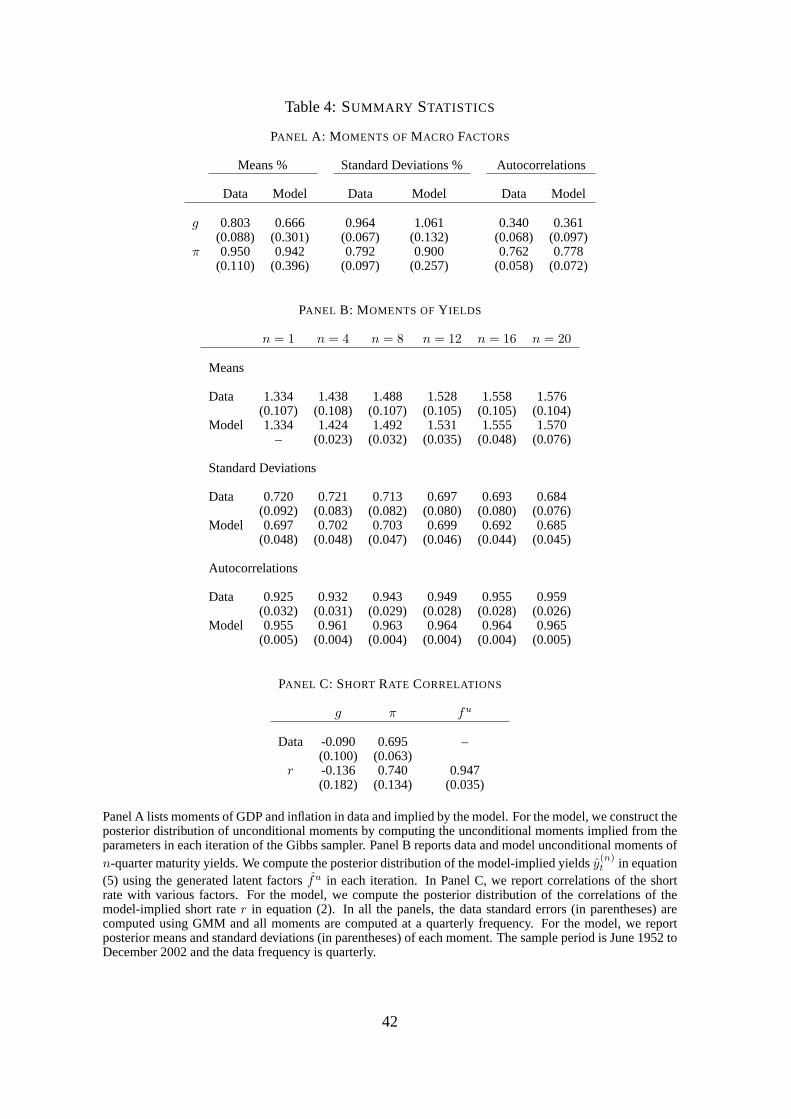
Table 4:SUMMARY STATISTICS

PANEL A: M OMENTS OFMACRO FACTORS

Means % Standard Deviations % Autocorrelations

Data Model Data Model Data Model

g 0.803 0.666 0.964 1.061 0.340 0.361(0.088) (0.301) (0.067) (0.132) (0.068) (0.097)

π 0.950 0.942 0.792 0.900 0.762 0.778(0.110) (0.396) (0.097) (0.257) (0.058) (0.072)

PANEL B: MOMENTS OFY IELDS

n = 1 n = 4 n = 8 n = 12 n = 16 n = 20

Means

Data 1.334 1.438 1.488 1.528 1.558 1.576(0.107) (0.108) (0.107) (0.105) (0.105) (0.104)

Model 1.334 1.424 1.492 1.531 1.555 1.570– (0.023) (0.032) (0.035) (0.048) (0.076)

Standard Deviations

Data 0.720 0.721 0.713 0.697 0.693 0.684(0.092) (0.083) (0.082) (0.080) (0.080) (0.076)

Model 0.697 0.702 0.703 0.699 0.692 0.685(0.048) (0.048) (0.047) (0.046) (0.044) (0.045)

Autocorrelations

Data 0.925 0.932 0.943 0.949 0.955 0.959(0.032) (0.031) (0.029) (0.028) (0.028) (0.026)

Model 0.955 0.961 0.963 0.964 0.964 0.965(0.005) (0.004) (0.004) (0.004) (0.004) (0.005)

PANEL C: SHORT RATE CORRELATIONS

g π fu

Data -0.090 0.695 –(0.100) (0.063)

r -0.136 0.740 0.947(0.182) (0.134) (0.035)

Panel A lists moments of GDP and inflation in data and implied by the model. For the model, we construct theposterior distribution of unconditional moments by computing the unconditional moments implied from theparameters in each iteration of the Gibbs sampler. Panel B reports data and model unconditional moments ofn-quarter maturity yields. We compute the posterior distribution of the model-implied yieldsy

(n)t in equation

(5) using the generated latent factorsfu in each iteration. In Panel C, we report correlations of the shortrate with various factors. For the model, we compute the posterior distribution of the correlations of themodel-implied short rater in equation (2). In all the panels, the data standard errors (in parentheses) arecomputed using GMM and all moments are computed at a quarterly frequency. For the model, we reportposterior means and standard deviations (in parentheses) of each moment. The sample period is June 1952 toDecember 2002 and the data frequency is quarterly.

42

Table 5:VARIANCE DECOMPOSITIONS

PANEL A: Y IELD LEVELS y(n)t

Proportion Risk Premia Variance Decompositions

Total Pure Risk PremiaPure Risk Including

Maturity (qtrs) Premia Covariances g π fu g π fu

One-Quarter Ahead1 0.0 0.0 14.5 59.2 26.3 – – –4 0.5 1.3 21.7 42.5 35.9 0.2 29.4 70.412 4.2 20.4 26.3 25.8 47.9 6.3 7.0 86.720 10.2 37.0 27.4 21.1 51.5 13.7 0.6 85.7

Four-Quarters Ahead1 0.0 0.0 23.5 46.3 30.2 – – –4 0.4 10.0 27.5 36.8 35.7 22.9 0.4 76.812 5.0 31.9 30.4 28.0 41.6 29.3 4.6 66.120 12.9 46.7 31.1 25.6 43.3 31.0 8.5 60.4

Unconditional1 0.0 0.0 29.9 33.8 36.4 – – –4 0.7 14.9 30.7 31.7 37.6 31.7 22.9 45.512 6.9 38.2 31.4 29.9 38.8 32.0 24.7 43.320 16.5 52.1 31.5 29.4 39.1 32.0 25.7 42.3

43

Table 5 Continued

PANEL B: Y IELD SPREADSy(n)t − y

(1)t

Proportion Risk Premia Variance Decompositions

Total Pure Risk PremiaPure Risk Including

Maturity (qtrs) Premia Covariances g π fu g π fu

One-Quarter Ahead4 19.3 38.3 8.3 86.0 5.7 0.2 29.4 70.412 21.3 24.2 2.5 93.0 4.6 6.3 7.0 86.720 22.9 1.3 1.4 95.4 3.3 13.7 0.6 85.7

Four-Quarters Ahead4 21.4 24.9 4.9 87.7 7.3 13.4 3.4 83.212 26.3 -11.1 1.6 92.8 5.6 24.4 0.2 75.420 28.3 -54.3 0.7 95.6 3.7 28.2 2.7 69.1

Unconditional4 23.1 16.2 3.9 88.1 8.0 21.2 0.6 78.212 28.2 -27.9 1.4 92.6 6.0 29.1 1.3 69.620 30.1 -79.6 0.5 95.6 3.9 31.3 4.7 64.0

PANEL C: EXPECTEDEXCESSRETURNS

One-Quarter Ahead Four-Quarters Ahead Unconditional

Maturity (qtrs) g π fu g π fu g π fu

4 11.9 49.1 39.0 1.5 21.8 76.7 8.7 11.2 80.212 23.2 59.1 17.7 1.6 52.1 46.3 0.4 41.7 58.020 25.4 60.5 14.1 3.4 58.9 37.7 0.0 50.9 49.1

The table reports variance decompositions of forecast variance (in percentages) for yield levels,y(n)t , in

Panel A; yield spreads,y(n)t − y

(1)t , in Panel B; and unconditional expected excess holding period returns,

E(rx(n)t+1) = E(ny

(n)t − (n− 1)y(n−1)

t+1 − rt), in Panel C. For yield levels and yield spreads, we also examinethe variance decomposition due to time-varying risk premia and predictability of state variablesXt. In PanelsA and B, we also attribute the total forecast variance into time-varying risk premia and EH components usingthe method outlined in Section 4.2. We partition the bond yield coefficientbn on Xt in equation (6) into anEH term and into a risk-premia term:bn = bEH

n + bRPn , wherebEH

n is computed by setting the prices of riskλ1 = 0. If ΩF,h represents the forecast variance of the factors at horizonh, then the the pure risk premiaproportion reportsbRP>

n ΩF,hbRPn /b>n ΩF,hbn, and the column that includes the covariance terms reports the

proportion1 − bEH>n ΩF,hbEH

n /b>n ΩF,hbn. The total variance decomposition is performed onb>n ΩF,hbn,while the pure risk premia decomposition is performed onbRP>

n ΩF,hbRPn . All maturities are in quarters. We

ignore observation error for computing variance decompositions for yield levels and yield spreads. All thevariance decompositions are computed using the posterior mean of the parameters listed in Table 2.

44

Table 6:CHARACTERIZING EXCESSRETURNS

PANEL A: FACTOR COEFFICIENTS

Maturity (qtrs)

4 8 12 16 20

Axn 0.002 0.004 0.006 0.008 0.009

Bxn g -0.016 -0.056 -0.101 -0.145 -0.189

π -0.056 -0.165 -0.282 -0.398 -0.512fu 0.117 0.244 0.358 0.468 0.574

PANEL B: PREDICTABILITY REGRESSIONS

Data Estimates Model-Implied Estimates

g π y(20) R2 g π y(20) R2

n = 4 -0.072 -0.078 0.223 0.036 -0.037 -0.051 0.163 0.034(0.064) (0.090) (0.096) (0.049) (0.087) (0.065)

n = 12 -0.193 -0.461 0.752 0.040 -0.171 -0.360 0.622 0.036(0.184) (0.240) (0.296) (0.175) (0.327) (0.217)

n = 20 -0.237 -0.719 1.129 0.039 -0.306 -0.678 1.040 0.037(0.266) (0.366) (0.450) (0.317) (0.598) (0.356)

In Panel A, we report the coefficients of the conditional expected excess holding period returnEt(rx(n)t+1 =

Axn+Bx>

n Xt defined in equation (8) on the factorsXt = (gt πt fut ). In Panel B, we regress one-quarter excess

holding period returns for ann-period bond,rx(n)t+1 onto GDP, inflation, and a bond yield. The standard errors

for the OLS estimates from data (in parentheses) are computed using robust standard errors. We compute themodel-implied coefficients andR2 as follows. We construct the posterior distributions of the model-impliedestimates by computing the implied coefficients from the model parameters in each iteration of the Gibbssampler. We report posterior means and standard deviations (in parentheses) of each coefficient. The datafrequency is quarterly and the sample period is June 1952 to December 2002.

45

Table 7:TAYLOR RULES

PANEL A: BENCHMARK TAYLOR RULE

Full Sample Pre-82:Q4 Post-82:Q4

OLS Model OLS Model OLS Model

const 0.007 0.009 0.006 0.009 0.007 0.011(0.001) (0.002) (0.001) (0.002) (0.002) (0.001)

gt 0.036 0.091 0.004 0.067 0.238 0.160(0.071) (0.064) (0.080) (0.073) (0.104) (0.109)

πt 0.643 0.322 0.677 0.352 0.605 0.253(0.080) (0.143) (0.082) (0.194) (0.130) (0.106)

PANEL B: BACKWARD-LOOKING TAYLOR RULE

const gt πt gt−1 πt−1 rt−1 R2

OLS 0.000 0.074 0.182 -0.005 -0.077 0.879 0.895(0.000) (0.027) (0.046) (0.029) (0.041) (0.035)

Model -0.000 0.091 0.322 -0.019 -0.218 0.931 0.976(0.001) (0.064) (0.143) (0.021) (0.092) (0.032)

PANEL C: FINITE-HORIZON FORWARD-LOOKING TAYLOR RULE

Forward-Looking Taylor Rule Coefficients Implied Short Rate Coefficients

const Et(gt+k,k) Et(πt+k,k) R2 δ1,g δ1,π δ1,fu

k = 1 0.007 0.151 0.509 0.117 0.074 0.331 0.587(0.003) (0.221) (0.154) (0.077) (0.122) (0.233)

k = 4 0.001 0.502 0.998 0.139 0.099 0.331 0.492(0.006) (0.417) (0.286) (0.052) (0.081) (0.146)

k = 8 -0.008 0.751 1.277 0.132 0.072 0.306 0.514(0.096) (5.096) (1.658) (0.083) (0.146) (0.284)

k = 20 -0.010 0.003 2.066 0.142 0.016 0.311 0.600(0.172) (6.878) (4.854) (0.089) (0.127) (0.224)

46

Table 7 Continued

PANEL D: INFINITE-HORIZON FORWARD-LOOKING TAYLOR RULE

Forward-Looking Taylor Rule Coefficients Implied Short Rate Coefficients

const gt πt β δ1,g δ1,π δ1,fu

k = ∞ -0.007 0.015 0.098 0.933 0.057 0.267 0.615(0.024) (0.034) (0.037) (0.036) (0.061) (0.078) (0.181)

PANEL E: FORWARD- AND BACKWARD-LOOKING TAYLOR RULE

const Et(gt+k,k) Et(πt+k,k) gt−1 πt−1 rt−1 R2

k = 1 -0.002 0.151 0.509 -0.013 -0.071 0.857 0.983(0.003) (0.221) (0.154) (0.029) (0.150) (0.057)

k = 4 -0.007 0.502 0.998 -0.014 -0.045 0.686 0.989(0.006) (0.417) (0.286) (0.016) (0.067) (0.163)

Panel A reports the OLS and model-implied estimates of the benchmark Taylor (1993) rule in equation (9)over the full sample and over subperiods; Panel B reports the backward-looking Taylor rule (10); Panel Creports the finite-horizon, forward-looking Taylor rule without discounting in equation (17); Panel D reportsthe infinite-horizon forward-looking Taylor rule with discounting in equation (19); and Panel E reports theforward- and backward-looking Taylor rule in equation (24). Panels C and D also report the implied short ratecoefficients corresponding to the forward-looking Taylor rules without discounting in equation (16) for eachhorizonk and equation (22) for the forward-looking Taylor rule with discounting. For the model-impliedcoefficients, we construct the posterior distribution of Taylor rule coefficients by computing the impliedcoefficients from the model parameters in each iteration of the Gibbs sampler. We report posterior meansand standard deviations (in parentheses) of each coefficient. The standard errors for the OLS estimates (inparentheses) are computed using robust standard errors. In each panel, the data frequency is quarterly and thefull sample period is June 1952 to December 2002.

47

Table 8:MONETARY POLICY SHOCKS

OLS Estimates Model-Implied Estimates

Fwd- Romer-Bmk Bwd Bmk Bwd Fwd Bwd Romer r ∆r

Correlations

OLS Benchmark Rule 1.000 0.454 0.807 0.340 0.814 0.344 0.276 0.713 0.140OLS Backward Rule 1.000 0.250 0.720 0.254 0.712 0.715 0.325 0.886Model Benchmark Rule 1.000 0.210 0.999 0.214 0.155 0.916 0.017Model Backward Rule 1.000 0.223 0.999 0.465 0.147 0.540Model Forward Rule 1.000 0.228 0.151 0.907 0.009Model Fwd-Bwd Rule 1.000 0.452 0.145 0.518Romer-Romer Shock 1.000 0.290 0.726Short Rater 1.000 0.187Change of Short Rate 1.000

Autocorrelations 0.743 -0.267 0.948 -0.195 0.942 -0.195 -0.183 0.924 -0.184

Standard Deviation 0.021 0.009 0.024 0.006 0.022 0.004 0.007 0.029 0.011

Minimum -0.049 -0.058 -0.042 -0.022 -0.040 -0.016 -0.040 0.006 -0.073

Maximum 0.094 0.043 0.085 0.024 0.079 0.018 0.025 0.154 0.037

The table reports summary statistics of OLS estimates and model-implied estimates of various Taylor rulespecifications. We denote the benchmark Taylor rule as “Bmk,” the forward-looking rule as “Fwd,”, thebackward-looking Taylor rule as “Bwd,” and the forward- and backward-looking Taylor rule as ”Fwd-Bwd.”The OLS estimates of benchmark and backward-looking Taylor rules are simply the residuals from equations(9) and (10), respectively. The no-arbitrage benchmark shock is the scaled latent factor,εMP,T in equation(9). The no-arbitrage backward-looking Taylor policy shocks are theεMP,B terms in (13). The no-arbitrageforward-looking Taylor rule shocks,εMP,F , are computed from equation (17) for a horizon ofk = 4 quarters.The no-arbitrage forward- and backward-looking Taylor rule residuals representεMP,FB from equation (24),also with ak = 4-quarter horizon. We construct the Romer and Romer (2004) measure of policy shocksconverted to a quarterly sequence by summing the monthly Romer-Romer shocks in Table 2 of Romer andRomer (2004). The last two columns report the correlations of the 1-quarter short rate,r, and the change inthe 1-quarter short rate,∆r. All monetary policy shocks and the short rate are annualized. The no-arbitrageshocks are computed using the posterior mean of the latent factors. The sample period is June 1952 toDecember 2002 and the data frequency is quarterly.

48

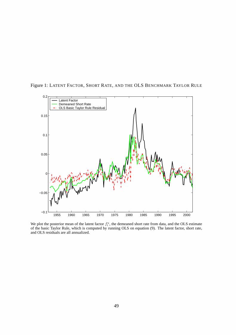
Figure 1:LATENT FACTOR, SHORT RATE, AND THE OLS BENCHMARK TAYLOR RULE

1955 1960 1965 1970 1975 1980 1985 1990 1995 2000−0.1

−0.05

0

0.05

0.1

0.15

0.2Latent FactorDemeaned Short RateOLS Basic Taylor Rule Residual

We plot the posterior mean of the latent factorfut , the demeaned short rate from data, and the OLS estimate

of the basic Taylor Rule, which is computed by running OLS on equation (9). The latent factor, short rate,and OLS residuals are all annualized.

49

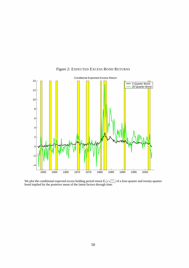
Figure 2:EXPECTEDEXCESSBOND RETURNS

1955 1960 1965 1970 1975 1980 1985 1990 1995 2000

−4

−2

0

2

4

6

8

10

12

14Conditional Expected Excess Return

4 Quarter Bond 20 Quarter Bond

We plot the conditional expected excess holding period returnEt[rx(n)t+1] of a four-quarter and twenty-quarter

bond implied by the posterior mean of the latent factors through time.

50

Figure 3:MONETARY POLICY SHOCKS

1955 1960 1965 1970 1975 1980 1985 1990 1995 2000−0.08

−0.06

−0.04

−0.02

0

0.02

0.04

0.06OLS Estimates

1955 1960 1965 1970 1975 1980 1985 1990 1995 2000−0.08

−0.06

−0.04

−0.02

0

0.02

0.04

0.06Model−Implied

In the top panel, we plot the OLS estimates of the residuals of the backwards-looking Taylor rule (equation(10)). The bottom panel plots the corresponding model-implied monetary policy shocks, which are theposterior mean estimates ofεMP,B

t = δ12u2t from equation (13). In both the top and bottom panels, we

plot annualized monetary policy shocks. NBER recessions are shown as shaded bars.

51

Figure 4:IMPULSE RESPONSES OFFACTORS

Model Implied Unrestricted VAR

0 5 10 15 20−0.4−0.2

00.20.40.60.8

1

1% GDP Shock

gπr

0 5 10 15 20−0.4−0.2

00.20.40.60.8

1

1% Inflation Shock

gπr

0 5 10 15 20−0.4−0.2

00.20.40.60.8

1

1% Short Rate Shock

gπr

0 5 10 15 20−0.4−0.2

00.20.40.60.8

1

1% GDP Shock

gπr

0 5 10 15 20−0.4−0.2

00.20.40.60.8

1

1% Inflation Shock

gπr

0 5 10 15 20−0.4−0.2

00.20.40.60.8

1

1% Short Rate Shock

gπr

The left (right) column shows the impulse response for the model (an unrestricted VAR). The unrestrictedVAR contains GDP growth, inflation, and the short rate. Ally-axis responses are in percentages, and weshow quarters on thex-axis. All initial shocks are 1% and are computed using a Cholesky decompositionthat orders the variables(gt, πt, f

ut ) in the model and(gt, πt, rt) in the unrestricted VAR. To produce the

bottom left-hand plot, we shock the latent factor in the model VAR in proportion so that the initial responseto the short rate is 1%.

52

Figure 5:IMPULSE RESPONSES OFY IELDS

0 5 10 15 200

0.25

0.5

0.75

1

1.25

1.5

yt(1)

gπr

0 5 10 15 200

0.25

0.5

0.75

1

1.25

1.5

yt(4)

gπr

0 5 10 15 200

0.25

0.5

0.75

1

1.25

1.5

yt(20)

gπr

0 5 10 15 20−0.2

0

0.2

yt(20)−y

t(1)

gπr

The panels show the responses of the one-, four- and twenty-quarter yield, and the term spread between thetwenty- and one-quarter yields to 1% shocks to GDP growthgt and inflationπt. We also plot the response ofa 1% shock in the short rate, which is computed by constructing a shock to the state variables proportionalto their Cholesky decomposition that sums to a 1% short rate shock. Yields on they-axis are annualized andwe show quarters on thex-axis. The impulse responses are computed using a Cholesky decomposition thatorders the variables(gt, πt, f

ut ).

53

Figure 6:IMPULSE RESPONSES FROMFORWARD-LOOKING TAYLOR RULES

0 2 4 6 8 10 12 14 16 18 20−0.16

−0.14

−0.12

−0.1

−0.08

−0.06

−0.04

−0.02

0GDP Response to 1% Latent Factor Shock

Basick=1k=4k=20

0 2 4 6 8 10 12 14 16 18 200

0.05

0.1

0.15

0.2

0.25

0.3

Inflation Response to 1% Latent Factor Shock

Basick=1k=4k=20

We plot impulse responses to GDP (top panel) and inflation (bottom panel) from benchmark Taylor rules andfrom forward-looking Taylor rules (finite horizon, without discounting) to a 1% shock in the latent factor,fu

t .Yields on they-axis are annualized and we show quarters on thex-axis. The impulse responses are computedusing a Cholesky decomposition that orders the variables(gt, πt, f

ut ).

54