Embed Size (px)
Citation preview
No-arbitrage, state prices and trade in thinfinancial markets 1
Andres Carvajal 2 Marek Weretka 3
October 26, 2007
1This is work in progress. A. Carvajal acknowledges the financial supportof a Warwick-RSS grant, and the hospitality of the Department of Economics atthe University of Wisconsin at Madison.
2CRETA and Department of Economics, University of Warwick, Coventry CV47AL, United Kingdom; Phone: +44-(0)2476-523040; Fax: +44-(0)2476-523032; e-Mail address: [email protected]
3University of Wisconsin-Madison, Department of Economics, 1180 Obser-vatory Drive, Madison, WI 53706. Phone: (608) 262 2265; e-Mail address:[email protected].
Abstract
When financial markets are competitive (infinitely deep), there can be noriskless and costless opportunities for profit; arbitrage opportunities are im-possible under equilibrium prices in competitive markets. In thin markets,however, trading positions exert significant price impacts, which could ren-der the classical analysis inapplicable. In this paper we examine how non-competitiveness in thin markets affects the choice of financial portfolios andthe determination of equilibrium prices. We apply a model of economic equi-librium based on [14], in which individual traders recognize and estimate theimpact of their trades on financial prices, and in which these effects are deter-mined endogenously as part of the equilibrium concept. The departure fromthe competitive model complicates the structure of equilibrium determina-tion, and none of the standard positive or normative results are immediatelyapplicable. The possibility of a no-arbitrage condition, and the derivationof state prices must now be argued. We concentrate on the case in whichmarkets allow for perfect insurance.
Key words: asset pricing; institutional traders; price impact; thin mar-kets; pricing kernel; Modigiliani-Miller neutrality.
JEL classification numbers: D43, D53, G11, G12, L13
The Arrow-Debreu model has been the basis of a very significant portion
of economic and financial research in the last decades. The model has served
as a flexible and general, yet parsimonious, tool for theoretical analysis, for
the development of applications, and for many policy recommendations.
The competitive model imposes the assumption that all agents interven-
ing in the market observe a price that they take as given: they assume
that their trade in the market, however large, can be made at that fixed
price. This assumption simplifies the definition and applications of economic
equilibrium, and yields important results such as the formalization of Adam
Smith’s “invisible hand” in the form of the First Fundamental Theorem of
Welfare Economics. The assumption has also been critically present in promi-
nent applications of the Arrow-Debreu model - the equilibrium asset pricing
models such as CAPM or consumption CAPM, for instance. Furthermore,
the theory of the determination of the prices of derivatives, and the formulae
derived from this theory and applied in practice, are based on the implication
that at equilibrium there should be no costless and riskless opportunities for
profit. Under this condition, asset prices embed an “objective” probability
distribution that can be used to obtain the price of any asset as its discounted
expected return: this is the basic content of the Fundamental Theorem of As-
set Pricing, of its applications (the Modigliani-Miller theorem, for instance),
and of the formulae developed to price financial derivatives (for example, the
Black-Scholes formula).
The assumption that all agents ignore the impact of their trades on prices,
however, appears at odds with empirical evidence from crucial markets. In
financial markets, even as deep as NYSE or NASDAQ, the evidence is clear
in this direction: large institutional traders have non-negligible price impacts
(see [6]), which they do take into account when designing their trading strate-
gies: they often spread their transactions over a number of days, in order to
ameliorate their impact on prices (see [2]), and tools have been developed
to implement portfolio recompositions taking into account their price im-
pacts.1 Importantly, these large traders constitute a very significant portion
1
of volume of trade in financial markets (see [3]).
Attempts to develop a general equilibrium framework in which traders do
take into account their price impacts have so far proved to be less successful
than the competitive counterpart. The work initiated by T. Negishi in [9],
though interesting, either required the oversimplification of assumptions, or
gave highly complex, intractable and inapplicable models: in the Negishi’s
approach, traders were allowed to have subjective perceptions of the price
impact, which implied a great deal of arbitrariness on the determination
of equilibria, unless the subjective conjectures where exogenously restricted;
later attempts to impose more structure to the definition of equilibrium en-
dowed the model with explicit strategic games, which came at the cost of
tractability.2
Nearly two decades ago, important literature on financial microstructure
emerged. In this strand of literature, price impacts of the traders result from
asymmetric information rather than from a small number of traders. These
models assume only one risky asset and they are consequently incapable of
addressing the question of no-arbitrage and arbitrage asset pricing.3
In this paper, we apply a model of economic equilibrium based on [14], in
which all individual traders recognize the impact that their trades have on
financial prices, and in which these effects are determined endogenously as
part of the equilibrium concept.4 We develop a model of noncompetitive fi-
nancial equilibrium that maintains the flexible, tractable and spare structure
of the Arrow-Debreu model.
The departure from the competitive model complicates the structure of
equilibrium determination, and none of the standard positive or normative
results are immediately applicable. The necessity of a no-arbitrage condition,
and the derivation of an objective probability have now to be argued. In this
paper, we concentrate on the case in which the existing financial markets
allow for complete insurance against risk; to the best of our knowledge, there
is no previous study of noncompetitive markets with many arbitrary assets
that possibly have collinear payoffs.
2
This paper is part of a research program in which we study the prop-
erties of abstract thin markets. As a part of this program, [15] shows that
the concept of equilibrium from this paper refines a Subgame Perfect Nash
equilibrium in the game defined by the Walrasian auction. There, it is also
argued that the equilibrium outcome will be observed in anonymous markets,
in which investors have no other information but their past trades and market
prices, and therefore they discover market power through a statistical infer-
ence by estimating slopes of their demands using the Least Squares method.
Therefore the equilibrium has a game theoretic foundation endowed with the
learning process by which anonymous markets converge to this equilibrium.
We believe that the assumption of anonymity is approximately satisfied in
financial markets, in which large institutional investors know that they have
price impacts, but very often have no information about those with whom
they are trading.
1 The economy
We study a financial market over two periods. In the second period, there is
a finite number of states of the world, which are indexed by s = 1, . . . , S. In
the first period, investors trade assets that deliver a numeraire return in the
second period. There is only one good, money, and all assets are denominated
in this commodity.
There is a finite number of assets, indexed by a = 1, . . . , A. Asset payoffs
are uncertain: in period one, asset a pays Ras in state s. Ra = (Ra
1, . . . , RaS)T
is a commonly-known random variable. R = (R1, . . . , RA), which is an S×A
matrix, denotes the asset structure of the economy.5
We restrict our attention to complete financial markets: we assume that
there are at least as many assets with linearly independent payoffs as states
of the world. Without further loss of generality, we assume that the first S
assets are linearly independent: we partition R = ( RS RA−S ), and assume
that the S × S matrix RS is nonsingular.
3
There is a finite number of (large) investors, who trade assets among
themselves; a typical investor is indexed by i = 1, . . . , I. Investor i is endowed
with a future wealth of eis > 0, contingent on the state of the world. We
denote by ei = (ei1, . . . , e
iS) the random variable representing investor i’s
future wealth.
Portfolios are denoted by Θi, so the future numeraire consumption (or
wealth) of investor i, if she decides to purchase portfolio Θi, is given by
ci = ei + RΘi, a random variable that we restrict to take strictly positive
values. In the second period, at state s, investor i values consumption cis
by a state-dependent utility index uis(c
is). We assume that the Bernoulli
function uis : R++ → R is twice continuously differentiable, differentiably
strictly monotonic and differentiably strictly concave, and satisfies Inada
conditions.6
Ex-ante, individual preferences are von Neumann-Morgenstern with re-
spect to future consumption, and quasilinear with respect to present con-
sumption: ex-ante preferences of investor i are represented by
U i(ci0, (c
i1, . . . , c
iS)) = ci
0 +∑
s
uis(c
is), (1)
where ci0 represents the amount of numeraire that trader i consumes in the
present, a possibly negative amount.
For notational simplicity, henceforth we write ui(ci) =∑
s uis(c
is). By our
assumptions, ∂ui(ci) � 0; we take this vector as a column. Also, ∂2ui(ci) is a
diagonal, negative definite matrix (that is, all its diagonal entries are strictly
negative, and all non-diagonal entries are zero).
The economy is completely characterized by the triple of a profile of
individual preferences, a profile of initial endowments and an asset payoff
structure: {U, e, R} = {(U i)i, (ei)i, R}.
4
2 Equilibrium in thin markets
In thin markets, investors are large relative to the average volume of trade,
and hence their trades exert non-negligible impacts on market prices.
We model price impacts in the following way: for each investor i, we
denote by M i an A×A, positive definite and symmetric matrix; the typical
element M ia,a′ measures individual i’s belief of how the price of asset a changes
when she expands her buy order for asset a′ by one share: the perceived price
change exerted by a perturbation ∆ to her portfolio is M i∆.
Unlike in a standard equilibrium asset pricing models such as CAPM or
consumption-CAPM, in thin markets agents know that they face inelastic as-
set demands. It will be a part of the definition of equilibrium that the profile
of individual beliefs is mutually consistent, in the sense that each matrix M i
correctly measures the price impacts of trader i, given the individual price
impacts perceived by all other traders in the market.
An informal, intuitive definition of equilibrium in thin financial markets
follows. The ideas of the definition are formalized immediately after, and a
formal definition of equilibrium is given at the end of the section.
From now on, P ∈ RA is used to denote the vector of asset prices: P =
(P1, . . . , PA)T. We denote individual portfolios by Θi, and a profile (Θi)i of
portfolios by Θ. We denote a profile (M i)i of price impact matrices by M .
Definition. An equilibrium in thin financial markets for economy
{U, e, R} is a triple consisting of a vector of asset prices, a profile of portfolios
and a profile of price impact matrices, (P , Θ, M), such that:
1. all markets clear:∑
i Θi = 0;
2. all traded portfolios are individually optimal, given the price impacts
perceived by agents: for each trader i, at prices P , trade Θi is optimal,
given that any other trade, Θi, would change prices to P +M i(Θi−Θi);
3. all perceived price impact matrices correctly estimate the effects of in-
dividual portfolio perturbations on the prices that would be required for
5
the rest of the market to optimally absorb them: for each trader i, small
perturbations to her portfolio, ∆i, uniquely define a price at which the
other traders of the market, given their price impacts, are willing to
supply ∆i to i, and the derivative of this mapping at equilibrium trade
Θi is M i.
The first condition in the definition is standard, as in the definition of
competitive equilibrium; the other two are not.
2.1 Stable individual trade
Each trader now perceives that her trade does affect prices, and takes these
impacts into account when designing her investment strategy. Optimality of
such strategy now requires that it maximize her ex-ante utility, given that
she faces a “downward-sloping” demand from the rest of the market, with
“slope” given by her perception of price impacts. To avoid confusion with
the competitive model, we refer to this condition as stability.
Definition 1. Given prices P and price impacts M i, portfolio Θi is stable
for individual i if it solves program
maxΘi
U i(−(P + M i(Θi − Θi)) ·Θi, ei + RΘi). (2)
The second condition in the definition of equilibrium is the requirement
that, for each trader, her trade should be stable given equilibrium prices and
her perceived price impacts at equilibrium trade.7 It requires that for each
trader, given her price impact, no deviation from the equilibrium trade be
able improve her ex-ante utility.
Notice that, given the assumption of strong concavity of preferences and
the condition that price impact matrices are to be positive definite, stability
of Θi, given (P, M i), is characterized by the condition
P + M iΘi = RT∂ui(ei + RΘi). (3)
6
2.2 Subequilibrium and consistent price impacts
The third condition of the definition of equilibrium requires the perceived
price impacts M i of all traders to be accurate estimates of their actual price
impacts, at least locally and to a first order, given the perceived price impacts
of every other trader.
Suppose that trader i demands a portfolio Θi. Unlike in a competitive
market, in which she would assume that her trade will bear no impact on
market prices, here she knows that prices must endogenously adjust to en-
courage other traders to (optimally) accommodate her trade. Consequently,
in this model markets clear and other investors respond optimally to prices,
even if one of the investors, i, is trading a suboptimal quantity of shares, Θi;
this feature is captured by the notion of subequilibrium in financial markets,
defined below.
Definition 2. Given an individual i and a profile of perceived price impacts
for all traders but i, M−i = (M j)j 6=i, a subequilibrium triggered by trade
Θi is a pair of prices and trades by all other investors, (P , Θ−i), such that:
1. all markets clear: Θi +∑
j 6=i Θj = 0;
2. all traders other than i act optimally: for each j 6= i, trade Θj is stable
given (P , M j).
For each i, let S i(Θi; M−i) be the set of all subequilibria triggered by
trade Θi, given that the other traders in the market perceive their price
impacts as M−i, and let P i(Θi; M−i) be the projection of that set into the
space of prices. If P i(Θi; M−i) is single-valued in a neighborhood of some
Θi, it defines, at least locally, an inverse demand function P i(Θi), faced by
trader i, given M−i. If such function is differentiable, trader i can estimate
its derivatives. The condition of consistency of price impact matrices is
that, at equilibrium, perceived price impacts should not be arbitrary: each
trader is able to estimate the slope of her real inverse demand, so that the
inverse demand function implicit in the condition of stability of her trade
7
is a correct first-order approximation to her real inverse demand, given the
estimations made by all other traders.8 This concept of mutual consistency
of price impact estimations, which completes the definition of equilibrium, is
formalized next.
Definition 3. A profile M of price impact matrices for all traders is mutu-
ally consistent given prices and trades (P , Θ) if, for each individual i, there
exist open neighborhoods N i(Θi) and N i(P ), and a function P i : N i(Θi) →N i(P ), such that:
1. function P i is differentiable;
2. locally, P i is the inverse demand faced by i: for every Θi ∈ N i(Θi),
P i(Θi; M−i) ∩N i(P ) = {P i(Θi)}; (4)
3. matrix M i is a correct estimation of the derivative of function P i at
Θi: ∂P i(Θi) = M i.
It is important to notice that consistency is imposed on the whole pro-
file of individual matrices, and not matrix by matrix: the second and third
conditions of the definition require that ∂ΘiP i(Θi; M−i) = M i.9 Intuitively,
consistent price impact matrices reflect the price changes needed to clear the
market for any small deviation Θi by trader i, given that other traders re-
spond rationally to market prices in any subequilibrium. This means that
each trader correctly estimates her price impact, to a first order, and incor-
porates this information into her individual decision problem; this contrasts
with the competitive model, in which traders incorrectly assume that their
price impacts are null. Put simply, traders in thin markets do not act (in-
correctly) as price takers, and behave as “slope takers” instead.
2.3 Equilibrium
The three principles of equilibrium in thin financial markets have now been
introduced: equilibrium is a triple of prices, trades and perceptions of price
8
impacts such that (i) all markets clear; (ii) all traders are acting optimally,
given the perception they hold of their price impacts; and (iii) these per-
ceptions are accurate estimates of the actual price impacts exerted by the
traders. For the sake or formality, we repeat the definition of equilibrium
next.
Definition 4. An equilibrium in thin financial markets for economy
{U, e, R} is a triple consisting of a vector of asset prices, a profile of traded
portfolios and a profile of price impact matrices, (P , Θ, M) such that:
1. all markets clear:∑
i Θi = 0;
2. for each trader i, trade Θi is stable given (P , M i);
3. the profile of price impact matrices M is mutually consistent, given
prices and trades (P , Θ).
Importantly, notice that at equilibrium all trades take place at prices P .
The following lemma provides a transparent characterization of equilibrium
for the case when there are no redundant assets in the market. For simplicity
of notation, given an array of I − 1 positive definite matrices, ∆ = (∆j)j∈J ,
let H(∆) denote the harmonic average of the array:
H(∆) = (I − 1)(∑j∈J
(∆j)−1)−1. (5)
Lemma 1. Suppose that R is nonsingular.10 Then, (P , Θ, M) is an equilib-
rium in thin financial markets for economy {U, e, A} if, and only if,
1.∑
i Θi = 0;
2. for each trader i, P + M iΘi = RT∂ui(ei + RΘi);
3. for each trader i,
M i =1
I − 1H((M j −RT∂2uj(ej + RΘj)R)j 6=i). (6)
9
Proof. Proof of Lemma 1 is in appendix A1.
The primary objective of this paper is to demonstrate that equilibrium in
thin financial markets is consistent with the standard no-arbitrage principle.
Therefore, we now review the concept of no-arbitrage, introduce a weaker
version of that principle, and also introduce a “no irrelevant impact” condi-
tion for price impact matrices, and discuss its implication for economies with
elementary securities.
3 Arbitrage and irrelevant price impacts
3.1 No-arbitrage
It is well known that in a competitive equilibrium it is impossible to find a
portfolio that (i) generates payoff that is non-negative in all possible states
of the world, and is positive in some; and (ii) has non-positive cost in the
present. This property of asset prices is known as a no-arbitrage condition:
Definition 5. A vector of asset prices P allows no arbitrage opportu-
nities if RΘ > 0 implies P ·Θ > 0.
It is also well known that price vector P allows no-arbitrage opportunities
if, and only if, there exists a vector of strictly positive “state prices,” p ∈ RS++,
that determines the value of income in each state of the world: P = RTp.
Consequently, the next lemma follows:
Lemma 2. The set of asset prices that allow no arbitrage opportunities is
the following convex, open, positive cone:
{P ∈ RA|∃p ∈ RS++ : P = RTp}. (7)
Proof. This result is well known, hence its proof is omitted.
10
We find it instructive to introduce a weaker condition of no-arbitrage: a
requirement that portfolios whose future return is zero in all states of the
world should have zero cost at market prices.
Definition 6. A vector of asset prices P allows no weak arbitrage op-
portunities if RΘ = 0 implies P ·Θ = 0.
The weaker no-arbitrage condition amounts to relaxing the requirement
that state prices be strictly positive, as in the following lemma.
Lemma 3. The set of asset prices that allow no weak arbitrage opportunities
is
{P ∈ RA|∃p ∈ RS : P = RTp}. (8)
Proof. Proof of Lemma 3 is in appendix A1.
In a competitive equilibrium both the strong and the weak notions of
no-arbitrage are satisfied, as long as there is at least one rational agent who
maximizes preferences. In the following sections we show that when markets
are thin, only the weak notion of no-arbitrage is implied by optimization of a
rational agent.11 In order to claim the strong no-arbitrage condition, one also
needs to invoke the market clearing condition. This is why the distinction
between the weak and strong conditions becomes important in the theory of
thin financial markets.
Henceforth, we say that a pair of vectors of prices (P, p) ∈ RA × RS
is R-associated if they satisfy P = RTp. By our assumption that mar-
kets are complete, it is immediate that (P, p) is R-associated only if p =
(RTS)−1(P1, . . . PS)T. Consequently, R-association of prices defines a bijec-
tion between the linear subspace of all asset prices P satisfying the weak
no-arbitrage condition, set (8), and RS. In case of a strong arbitrage such
bijection is between a convex cone, set (7), and RS++.
If (P, p) is R-associated and P allows no arbitrage opportunities in the
strong sense, then vector (∑
s ps)−1p � 0 is a probability measure often
referred to as the pricing kernel implied by P . Similarly, if P allows no weak
11
arbitrage opportunities, then vector p can be interpreted as a (weak) pricing
kernel implied by P . Note, however, that the weak pricing kernel does not
have to be a probability measure since prices do not necessarily sum up to
one and for some states they can even take negative values.
3.2 Price impact
In this section we give an analogous result for price impact matrices. We call
it a “no irrelevant impact” condition: it is the requirement that only trades
of portfolios with non-zero future payoff should affect prices.
Definition 7. A price impact matrix M i gives no irrelevant impact if
RΘi = 0 implies M iΘi = 0.
Technically, M i gives no irrelevant impact if, and only if, the kernel of
matrix M i contains the kernel of matrix R. The no irrelevant impact condi-
tion implies that only trades of portfolios resulting in changes in consumption
may affect prices. The condition can be equivalently restated as the require-
ment that portfolios with identical payoffs should have identical price effects
and hence an agent is not subject to an asset illusion.12
The next result provides a unique decomposition for symmetric matrices
that give no irrelevant price impact. For any M i define mi = (RTS)−1M i
S(RS)−1,
where M iS is the S × S leading principal minor of matrix M i.
Lemma 4. Let M i be an A×A, symmetric price impact matrix. If M i gives
no irrelevant impact, then
1. M i can be written as M i = RT miR;
2. mi is the only matrix that allows for such decomposition of M i.
Proof. Proof of Lemma 4 is in appendix A1.
In the same vein as with prices, we say that a pair of an A × A matrix
and an S × S matrix (M i, mi) is R-associated, if M i = RTmiR. From
12
Lemma 4, it follows that if M i is symmetric and gives no irrelevant price
impacts, then (M i, mi) is R-associated if, and only if, mi = (RTS)−1M i
S(RS)−1.
Consequently, R-association defines a bijection between these sets of A× A
and S × S matrices.
Some other implications of the condition of no irrelevant price impact are
given next. The first two results show that the presence of one trader that
maximizes preferences and whose trade has no irrelevant impact is sufficient
for the weak no-arbitrage condition.
Proposition 1. Suppose that price impact matrix M i gives no irrelevant
price impact, and that there exists a portfolio Θi that is stable for i given
(P , M i). Then prices P allow no weak arbitrage opportunities.
Proof. By stability of individual trade, it follows that
P + M iΘi = RT∂ui(ei + RΘi). (9)
Multiplying (9) by any Θi such that RΘi = 0 gives
P ·Θi = ∂ui(ei + RΘi)TRΘi − (Θi)TM iΘ = 0, (10)
where the last equality follows from the fact that M i gives no irrelevant price
impact.
Intuitively, changes in the portfolio that do not affect payoffs do not
alter consumption either, and, hence, do not change the marginal rate of
substitution between assets. Since, at an optimum, the marginal rate of
substitution equals marginal revenue, P + M iΘi, the latter is not affected
either. But, with no irrelevant impact, marginal revenue is constant only
if prices are orthogonal to zero-payoff portfolios. The following corollary is
immediate
Corollary 1. If (P , Θ, M) is an equilibrium in thin financial markets for
{U, e, R}, and for at least one trader i price impact matrix M i gives no
13
irrelevant impact, then P allows no weak arbitrage opportunities, and there
exists a (weak) pricing kernel p ∈ RS such that P = RTp.
Proof. This follows from Proposition 1 and Lemma 3.
The next result demonstrates that, in equilibrium, if all traders but i es-
timate that they have no irrelevant price impact, then trader i automatically
has no irrelevant impact. Consequently asset illusion may occur only as a
global phenomenon, in which the irrelevant impact of a trader arises only
because of the asset illusion by other traders.
Proposition 2. Let (P , Θ, M) be an equilibrium in thin financial markets
for economy {U, e, R}. If for all traders j 6= i matrix M j gives no irrelevant
price impact, then matrix M i gives no irrelevant impact.
Before the proof of the proposition, we introduce a useful lemma, whose
proof we again defer to appendix A1.
Lemma 5. Return-equivalent deviations trigger the same subequilibrium prices:
Fix an individual i and a profile of perceived price impacts for all traders but
i, M−i = (M j)j 6=i, and suppose that each matrix M j gives no irrelevant price
impact. Suppose that portfolios Θi and Θi are return-equivalent, in the sense
that RΘi = RΘi. If (P , Θ−i) is a subequilibrium triggered by trade Θi, then(P , (Θj + (I − 1)−1(Θi − Θi))j 6=i
)(11)
is a subequilibrium triggered by trade Θi.
Proof of proposition 2. Let Θi be an arbitrary portfolio such that RΘi = 0.
By definition of equilibrium, there exists a local inverse demand function
P i. Then, we can define ϕ(λ) = P i(Θi + λΘi), for real numbers λ close
enough to 0. By lemma 5, it follows that, for any λ ∈ R, (P , (Θj − (I −1)−1λΘi)j 6=i) is a subequilibrium triggered by trade λΘi. Thus, for any λ,
subequilibrium prices are not affected, so it is immediate that ϕ′(λ) = 0,
14
while, by construction,
ϕ′(0) = ∂P i(Θi)Θi = M iΘi. (12)
Consequently, M i gives no irrelevant impact.
In this paper we restrict our attention to equilibria in which there is
no asset illusion and hence all price impact matrices satisfy no irrelevant
impact. In the following sections we argue that such equilibria exist and are
determinate. We conjecture that equilibria in which traders have irrelevant
impact do not exist. As of yet, however, we are not able to give a formal
argument to support our claim, leaving it as an open question for future
research.
4 Pricing kernel in thin complete markets
4.1 Elementary securities
A thin financial market is completely characterized by a triple consisting of
the utility functions of the traders, their initial endowments and the asset
payoffs structure, {U, e, R}. Since we are considering only the case of com-
plete financial markets, we can obtain a canonical auxiliary representation
by endowing the market with a complete set of elementary (Arrow) securi-
ties, in lieu of the set of securities R. That is, the representation of economy
{U, e, R} in elementary securities is economy {U, e, IS}.In the representation, we maintain the assumptions that markets are thin:
traders continue to realize that their trades do have price impacts, and they
estimate these impacts and take them into account at the moment of design-
ing their portfolios. For notational simplicity, we use lower-case characters for
the corresponding (endogenous) variables in the representation in elementary
securities:
Definition 8. Given preferences and endowments {U, e}, a triple consisting
15
of a vector of state prices, a profile of revenue transfers across states of the
world and a profile of state-price impact matrices, (p, θ, m) is an equilibrium
in elementary securities for {U, e} if it is an equilibrium in thin financial
markets for economy {U, e, IS}.
The following results are important: under our assumptions, equilibria in
elementary securities exist and are (generically) locally unique.
Proposition 3. Suppose there are at least three traders in the market. Then,
1. For any profile of preferences and endowments, {U, e}, there exists an
equilibrium in elementary securities (p, θ, m) such that all price impact
matrices mi are diagonal and positive definite.
2. If, moreover, all preferences are three times continuously differentiable,
then, typically in the space of preferences and endowments, all equilibria
in elementary securities with diagonal, positive-definite price impact
matrices are locally unique (i.e., isolated from one another).13
Proof. These results follow, respectively, from Theorems 1 and 2 in [14]. For
the sake of simplicity and completeness, appendix A2 specializes the proofs
to the case treated here.
Our result shows that the thin market model always gives some predic-
tions, and, furthermore, that these predictions are typically sharp, in the
sense that they pin down the outcome of the market, at least at a local level.
It is natural to ask whether in the equilibria resulting from Proposition 3
there are arbitrage opportunities and irrelevant price impacts. Observe that
in the economy with elementary securities the only portfolio that gives zero
return in all states is a zero portfolio, and obviously both the cost of such
portfolio and its price impact are zero, regardless of the specific prices and
price impact matrices. Therefore equilibrium prices do not allow for weak
arbitrage opportunities and there is no irrelevant price impact in the economy
16
with elementary securities. The more challenging question of whether the no-
arbitrage condition holds in the strong sense (so that a strong pricing kernel
exists) is addressed in the next proposition.
Proposition 4. Let (p, θ, m) be an equilibrium in elementary securities in
{U, e} with diagonal, positive definite price impact matrices mi. Then, prices
p allow no-arbitrage opportunities: p � 0
Proof. For every trader i, it must be true that p = ∂ui(ei + θi) − miθi. For
asset (state) s, since mi is diagonal, the latter means that ps = ∂uis(e
is +
θis)− mi
s,sθis. By market clearing, there must exist i for whom θi
s ≤ 0, which
means, by monotonicity of ui and positive definiteness of mi, that ps > 0.
Critically, the implication of Proposition 4 does not follow simply from the
existence of one rational trader with monotone preferences; rather, it follows
from the facts that traders’ von Neumann-Morgenstern utility functions are
separable and all markets clear. [16] provides examples of economies with
traders characterized by non-separable utility functions; there, one might
observe negative prices for some states of the world, even with preferences
that are strictly monotone. In such case negative prices result from cross-
market effects associated with market power.
4.2 Equivalence of the two representations
In this section we exploit market completeness to obtain a characterization of
equilibrium in economy {U, e, R}, by associating it with an equilibrium in the
corresponding economy endowed with the full set of elementary securities.
We say that a pair of portfolios (Θi, θi) ∈ RA × RS is R-associated if
the two portfolios are payoff equivalent, RΘi = θi. By market completeness,
for every θi there is at least one Θi such that (Θi, θi) is R-associated, for
example
Θi =
(R−1
S θi
0
). (13)
17
When there are no redundant assets, such Θi is unique. Note, however, that
the association of portfolios is not a bijection in general.
Further, we say that a triple of a vector of prices, a profile of portfolios,
and a profile of price impact matrices in market R, and a corresponding triple
in elementary securities are R-associated if so are each of their components:
(P, Θ, M) and (p, θ,m) are R-associated if:
1. the pair of prices (P, p) is R-associated: P = RTp;
2. for each i, the pair of portfolios (Θi, θi) is R-associated: RΘi = θi;
3. for each i, the pair of price impact matrices (M i, mi) is R-associated:
M i = RTmiR.
The next lemma establishes the connection between the equilibria in
economies with arbitrary assets and their counterparts with elementary se-
curities.
Lemma 6. Suppose that (P , Θ, M) and (p, θ, m) are R-associated. Then,
1. if (p, θ, m) is an equilibrium in elementary securities for {U, e} and∑i Θ
i = 0, then (P , Θ, M) is an equilibrium in thin financial markets
for {U, e, R};
2. if (P , Θ, M) is an equilibrium in thin financial markets for {U, e, R},then (p, θ, m) is an equilibrium in elementary securities for {U, e}.
Proof. Proof of Lemma 6 is in appendix A1.
In the following sections we explore the theoretic and practical implica-
tions of this result.
4.3 Equilibria with no-arbitrage
Noncompetitive behavior is inconsistent with the standard argument by which
no-arbitrage14 arises as a necessary condition for equilibrium in financial mar-
kets. In fact, no-arbitrage is an immediate implication of the existence of just
18
one rational, competitive trader. But if traders are noncompetitive, the argu-
ment fails: suppose that a trader i has chosen a portfolio Θi, even though an
arbitrage opportunity Θ exists in the market; if i were competitive, portfolio
Θi + λΘ, for any λ > 0 would give her more utility, whatever her prefer-
ences. But this need not be the case for noncompetitive i, for her demand
for portfolio Θ, the arbitrage opportunity, may exert ‘detrimental’ effects of
the price of Θ itself, and on the cost of portfolio Θi; while the first effect is
of second order, and hence vanishes for small λ, the second effect is of first
order.
This is an important issue, as no-arbitrage conditions and their impli-
cations in terms of existence and positivity of state prices constitute the
analytical basis for asset pricing theory.
Proposition 4 has given a condition under which no-arbitrage remains a
necessary condition of equilibria under noncompetitive behavior, for the case
of a full set of elementary securities. The following result is the most impor-
tant one in the paper: it shows that in economies with complete markets and
separable preferences, noncompetitive behavior is not incompatible with the
existence of a pricing kernel.
Theorem 1. Suppose that there are at least three traders in the market.
Then,
1. For any economy {U, e, R}, there exists an equilibrium (P , Θ, M) sat-
isfying that
(a) price impact matrices M i are symmetric, positive definite and give
no irrelevant price impact;
(b) prices P allow no strong (and, hence, no weak) arbitrage oppor-
tunities, and a classical pricing kernel exists.
2. If, moreover, all preferences are three times continuously differentiable,
then, for a typical profile of preferences and endowments {U, e}, and
any asset payoffs structure R, equilibria satisfying conditions (a) and
19
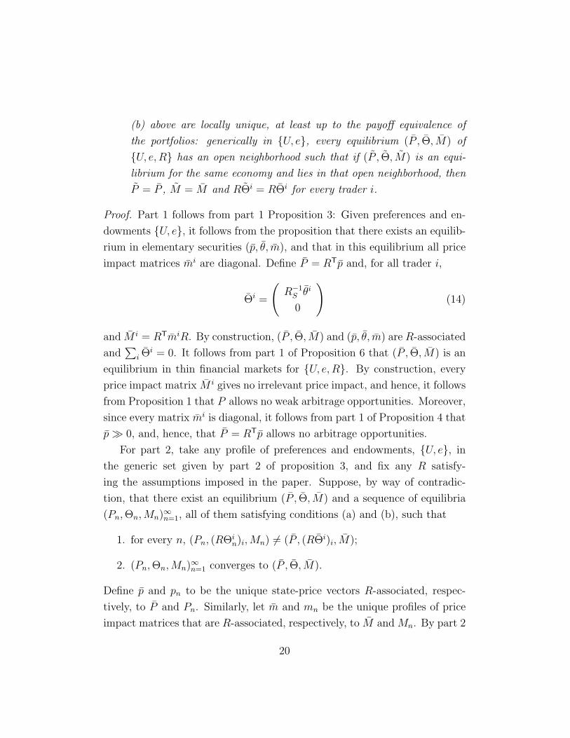
(b) above are locally unique, at least up to the payoff equivalence of
the portfolios: generically in {U, e}, every equilibrium (P , Θ, M) of
{U, e, R} has an open neighborhood such that if (P , Θ, M) is an equi-
librium for the same economy and lies in that open neighborhood, then
P = P , M = M and RΘi = RΘi for every trader i.
Proof. Part 1 follows from part 1 Proposition 3: Given preferences and en-
dowments {U, e}, it follows from the proposition that there exists an equilib-
rium in elementary securities (p, θ, m), and that in this equilibrium all price
impact matrices mi are diagonal. Define P = RTp and, for all trader i,
Θi =
(R−1
S θi
0
)(14)
and M i = RTmiR. By construction, (P , Θ, M) and (p, θ, m) are R-associated
and∑
i Θi = 0. It follows from part 1 of Proposition 6 that (P , Θ, M) is an
equilibrium in thin financial markets for {U, e, R}. By construction, every
price impact matrix M i gives no irrelevant price impact, and hence, it follows
from Proposition 1 that P allows no weak arbitrage opportunities. Moreover,
since every matrix mi is diagonal, it follows from part 1 of Proposition 4 that
p � 0, and, hence, that P = RTp allows no arbitrage opportunities.
For part 2, take any profile of preferences and endowments, {U, e}, in
the generic set given by part 2 of proposition 3, and fix any R satisfy-
ing the assumptions imposed in the paper. Suppose, by way of contradic-
tion, that there exist an equilibrium (P , Θ, M) and a sequence of equilibria
(Pn, Θn, Mn)∞n=1, all of them satisfying conditions (a) and (b), such that
1. for every n, (Pn, (RΘin)i, Mn) 6= (P , (RΘi)i, M);
2. (Pn, Θn, Mn)∞n=1 converges to (P , Θ, M).
Define p and pn to be the unique state-price vectors R-associated, respec-
tively, to P and Pn. Similarly, let m and mn be the unique profiles of price
impact matrices that are R-associated, respectively, to M and Mn. By part 2
20
of lemma 6, it follows that (p, (RΘi)i, m) and all (pn, (RΘin)i, mn) are equilib-
ria in elementary securities for {U, e}. Since R-association of prices and price
impact matrices both define bijections, it follows from the first property above
that for every n, (pn, (RΘin)i, mn) 6= (p, (RΘi)i, m). By the second property
above, (pn, (RΘin)i, mn) converges to (p, (RΘi)i, m), but this is impossible
since all equilibria in elementary securities for {U, e} are locally unique.
5 Thin financial markets and asset prices
5.1 The fundamental theorem of asset pricing
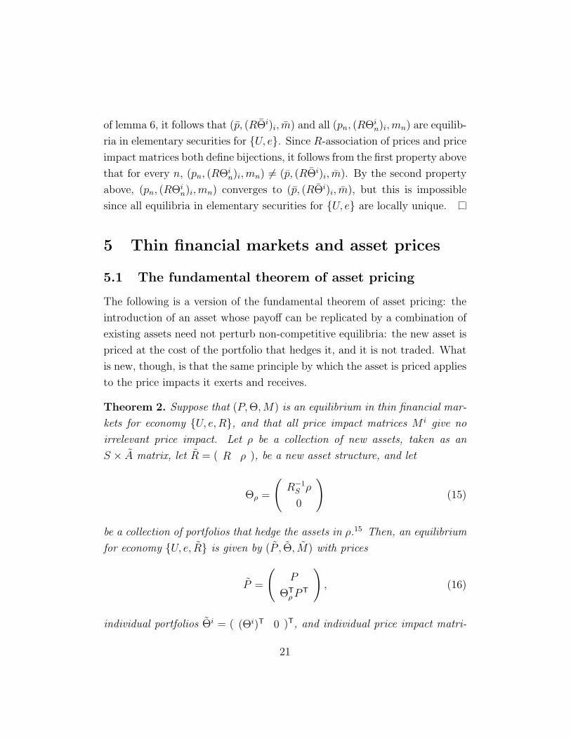
The following is a version of the fundamental theorem of asset pricing: the
introduction of an asset whose payoff can be replicated by a combination of
existing assets need not perturb non-competitive equilibria: the new asset is
priced at the cost of the portfolio that hedges it, and it is not traded. What
is new, though, is that the same principle by which the asset is priced applies
to the price impacts it exerts and receives.
Theorem 2. Suppose that (P, Θ, M) is an equilibrium in thin financial mar-
kets for economy {U, e, R}, and that all price impact matrices M i give no
irrelevant price impact. Let ρ be a collection of new assets, taken as an
S × A matrix, let R = ( R ρ ), be a new asset structure, and let
Θρ =
(R−1
S ρ
0
)(15)
be a collection of portfolios that hedge the assets in ρ.15 Then, an equilibrium
for economy {U, e, R} is given by (P , Θ, M) with prices
P =
(P
ΘTρ PT
), (16)
individual portfolios Θi = ( (Θi)T 0 )T, and individual price impact matri-
21
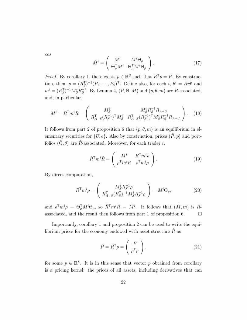
ces
M i =
(M i M iΘρ
ΘTρ M i ΘT
ρ M iΘρ
). (17)
Proof. By corollary 1, there exists p ∈ RS such that RTp = P . By construc-
tion, then, p = (RTS)−1(P1, . . . , PS)T. Define also, for each i, θi = RΘi and
mi = (RTS)−1M i
SR−1S . By Lemma 4, (P, Θ, M) and (p, θ,m) are R-associated,
and, in particular,
M i = RTmiR =
(M i
S M iSR−1
S RA−S
RTA−S(R−1
S )TM iS RT
A−S(R−1S )TM i
SR−1S RA−S
). (18)
It follows from part 2 of proposition 6 that (p, θ,m) is an equilibrium in el-
ementary securities for {U, e}. Also by construction, prices (P , p) and port-
folios (Θ, θ) are R-associated. Moreover, for each trader i,
RTmiR =
(M i RTmiρ
ρTmiR ρTmiρ
). (19)
By direct computation,
RTmiρ =
(M i
SR−1S ρ
RTA−S(RT
S)−1M iSR−1
S ρ
)= M iΘρ, (20)
and ρTmiρ = ΘTρ M iΘρ, so RTmiR = M i. It follows that (M,m) is R-
associated, and the result then follows from part 1 of proposition 6.
Importantly, corollary 1 and proposition 2 can be used to write the equi-
librium prices for the economy endowed with asset structure R as
P = RTp =
(P
ρTp
). (21)
for some p ∈ RS. It is in this sense that vector p obtained from corollary
is a pricing kernel: the prices of all assets, including derivatives that can
22
be replicated from existing assets, can be expressed as the value of their
returns at state prices p. Crucially, proposition 1 established the existence
of equilibria in which p is a pricing kernel in the classical sense (p � 0) and
can be used to define a probability measure over states of the world.
Notice, finally, that the computation of price impact matrices can be
obtained via their analogous in elementary securities as well: this is the
intuition of equation 19. In this sense, one can view the price impact matrices
in elementary securities as “price impact kernels.”
5.2 The interest rate puzzle
It follows by definition that in noncompetitive markets asset prices may di-
verge from competitive prices. We now ask whether such price biases can,
at least partially, explain discrepancies between the returns predicted by a
competitive model (the representative agent model) and the ones observed
empirically.
The risk-free interest rate puzzle was first observed by [13]. In short,
in the competitive theory of asset pricing, the risk-averse agents prefer flat
consumption over time. They are willing to postpone consumption only if
compensated by a high interest rate. Given the standard preferences, the
empirically observed growth rate of per capita consumption equal to 2%
cannot be reconciled with the risk-free interest rate of only 1%.
It follows from the Fundamental Theorem of Asset Pricing that with a
pricing kernel, the return to a riskless asset, 1 + r, can be computed as
the inverse of the sum of all state prices. The next proposition shows that
if one assumes that all individuals have identical CRRA Bernoulli utility
functions,16 then trade in financial markets results in an risk-free interest
rate that is below the one from a competitive model.
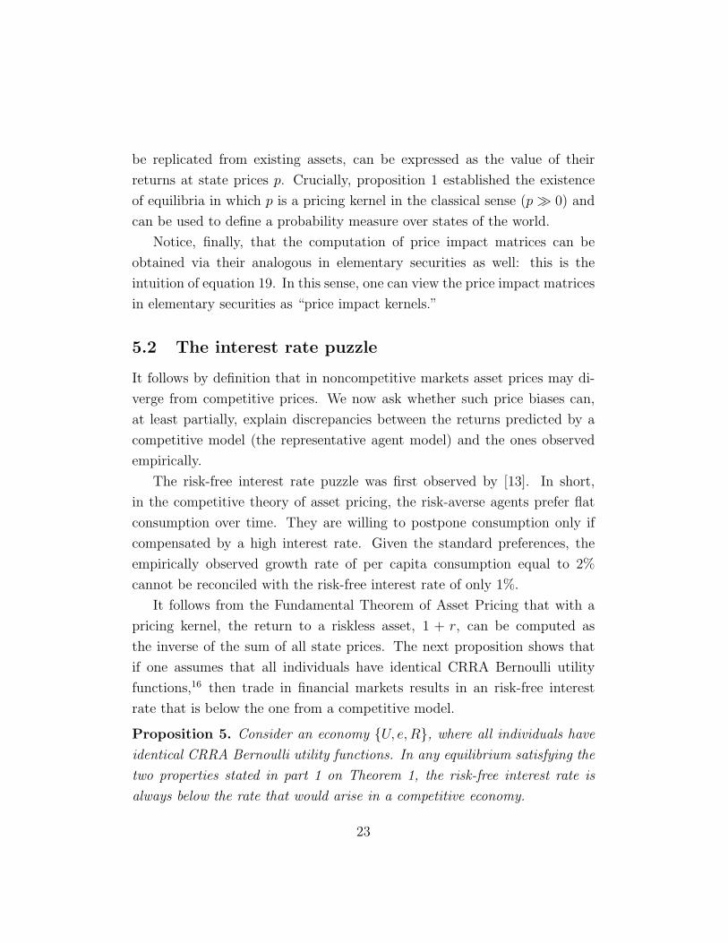
Proposition 5. Consider an economy {U, e, R}, where all individuals have
identical CRRA Bernoulli utility functions. In any equilibrium satisfying the
two properties stated in part 1 on Theorem 1, the risk-free interest rate is
always below the rate that would arise in a competitive economy.
23
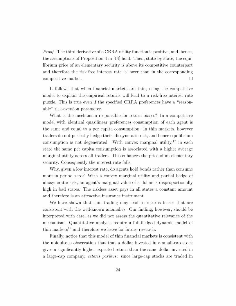
Proof. The third derivative of a CRRA utility function is positive, and, hence,
the assumptions of Proposition 4 in [14] hold. Then, state-by-state, the equi-
librium price of an elementary security is above its competitive counterpart
and therefore the risk-free interest rate is lower than in the corresponding
competitive market.
It follows that when financial markets are thin, using the competitive
model to explain the empirical returns will lead to a risk-free interest rate
puzzle. This is true even if the specified CRRA preferences have a “reason-
able” risk-aversion parameter.
What is the mechanism responsible for return biases? In a competitive
model with identical quasilinear preferences consumption of each agent is
the same and equal to a per capita consumption. In thin markets, however
traders do not perfectly hedge their idiosyncratic risk, and hence equilibrium
consumption is not degenerated. With convex marginal utility,17 in each
state the same per capita consumption is associated with a higher average
marginal utility across all traders. This enhances the price of an elementary
security. Consequently the interest rate falls.
Why, given a low interest rate, do agents hold bonds rather than consume
more in period zero? With a convex marginal utility and partial hedge of
idiosyncratic risk, an agent’s marginal value of a dollar is disproportionally
high in bad states. The riskless asset pays in all states a constant amount
and therefore is an attractive insurance instrument.
We have shown that thin trading may lead to returns biases that are
consistent with the well-known anomalies. Our finding, however, should be
interpreted with care, as we did not assess the quantitative relevance of the
mechanism. Quantitative analysis require a full-fledged dynamic model of
thin markets18 and therefore we leave for future research.
Finally, notice that this model of thin financial markets is consistent with
the ubiquitous observation that that a dollar invested in a small-cap stock
gives a significantly higher expected return than the same dollar invested in
a large-cap company, ceteris paribus : since large-cap stocks are traded in
24
deeper markets, the difference in returns is a premium for market depth (or
liquidity). Such premium cannot be reconciled with the competitive theory,
while it naturally arises in the model of thin trading.
6 A (very) simple example
We now use a “coconut” example to illustrate numerical differences between
equilibria in competitive economies and equilibria in thin financial markets.
We use this computations to illustrate that noncompetitiveness may help in
explaining well-known asset pricing puzzles, such as the risk-free interest rate
puzzle. Finally we show how Theorem 2 can be applied to price derivatives
in thin markets.
6.1 The economy
Consider an island where the only production technology available is coconut
palms. There are three equally likely states of the world, s = 1, 2, 3: in state
1 there is a drought in the north of the island and the palms there are not
productive; in state 2, the drought is in the south of the island; in state
3, there is no drought anywhere in the island, and in this case each palm
produces two coconuts.
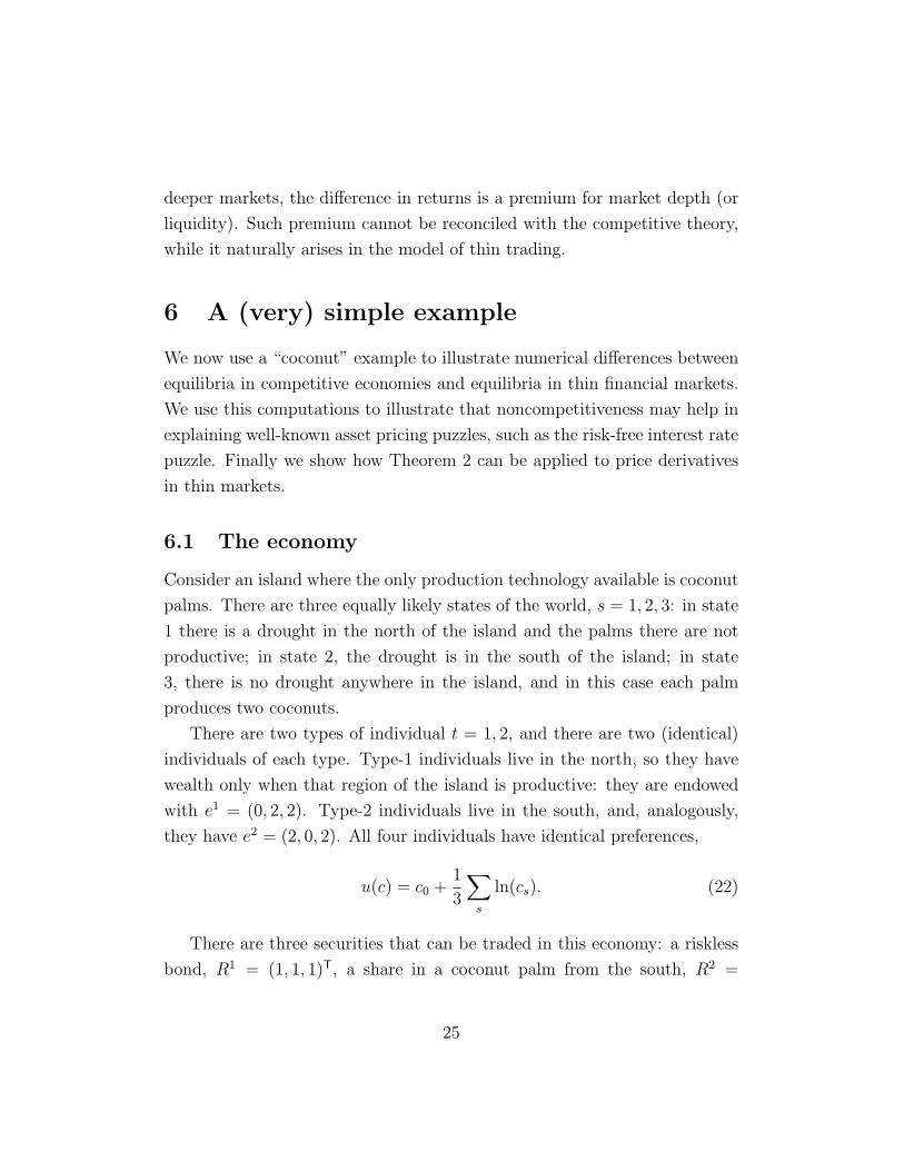
There are two types of individual t = 1, 2, and there are two (identical)
individuals of each type. Type-1 individuals live in the north, so they have
wealth only when that region of the island is productive: they are endowed
with e1 = (0, 2, 2). Type-2 individuals live in the south, and, analogously,
they have e2 = (2, 0, 2). All four individuals have identical preferences,
u(c) = c0 +1
3
∑s
ln(cs). (22)
There are three securities that can be traded in this economy: a riskless
bond, R1 = (1, 1, 1)T, a share in a coconut palm from the south, R2 =
25
(0, 2, 2)T, and a share in a coconut palm from the north, R3 = (2, 0, 2)T.
6.2 Equilibrium in thin financial markets
If all traders ignore their price effects and behave competitively, the equi-
librium in these financial markets is at prices P = (5/6, 1, 1)T, with both
type-1 individuals buying a portfolio Θ1 = (0,−1/2, 1/2)T and both type-2
individuals selling that portfolio.
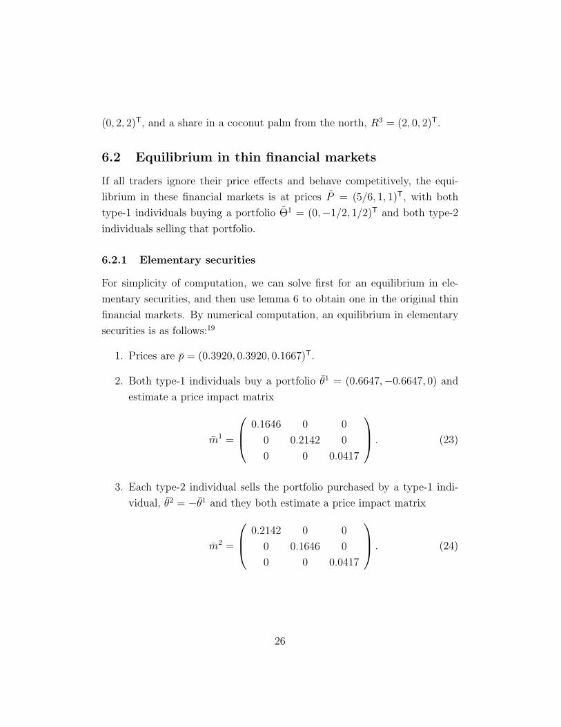
6.2.1 Elementary securities
For simplicity of computation, we can solve first for an equilibrium in ele-
mentary securities, and then use lemma 6 to obtain one in the original thin
financial markets. By numerical computation, an equilibrium in elementary
securities is as follows:19
1. Prices are p = (0.3920, 0.3920, 0.1667)T.
2. Both type-1 individuals buy a portfolio θ1 = (0.6647,−0.6647, 0) and
estimate a price impact matrix
m1 =
0.1646 0 0
0 0.2142 0
0 0 0.0417
. (23)
3. Each type-2 individual sells the portfolio purchased by a type-1 indi-
vidual, θ2 = −θ1 and they both estimate a price impact matrix
m2 =
0.2142 0 0
0 0.1646 0
0 0 0.0417
. (24)
26

6.2.2 Equilibrium
We can now use lemma 6 to compute the equilibrium with asset structure
R = (R1, R2, R3):
1. Prices are given by
P = RTp = (0.9507, 1.1173, 1.1173)T. (25)
2. Each individual of type 1 buys a portfolio
Θ1 = R−1θ1 =
0.0000
−0.3324
0.3324
, (26)
which is sold by a type-2 individual: Θ2 = −Θ1.
3. Each individual of type 1 estimates that her price impacts are
M1 = RTm1R =
0.4205 0.5117 0.4126
0.5117 1.0233 0.1667
0.4126 0.1667 0.8252
, (27)
while each individual of type 2 estimates
M2 = RTm2R =
0.4205 0.4126 0.5117
0.4126 0.8252 0.1667
0.5117 0.1667 1.0233
. (28)
One can readily verify that these values satisfy all the conditions of lemma
1, and, hence, constitute an equilibrium for {U, e, R}.
27
6.3 Price biases
Notice that in this economy the competitive risk-free interest rate is r =
1/P1 − 1 = 0.2. Importantly, notice that when these agents recognize their
price impacts the risk-free interest rate is lower: it is r = 1/P1 − 1 = 0.0519.
Another anomaly robustly documented in the empirical literature is the
equity premium puzzle: [8] has shown that over the last century the aver-
age annual return to stocks has been six percentage points above the annual
risk-free return to Treasury bills. Under reasonable risk preferences, the co-
variance of risky returns with per capita consumption growth cannot explain
an equity premium that high.
In our example, if trade were competitive the equity premium would be,
for asset 2,E(R2)
P2
− r = 0.1333. (29)
In the equilibrium in thin markets, the same return is traded at a higher
premiumE(R2)
P2
− r = 0.1414. (30)
Therefore in thin markets the equity premium is significantly above the one
obtained in the competitive setting. Intuitively, price impacts of the traders
are the highest for elementary securities corresponding to “bad” states of the
economy, and for such states the price biases are the strongest.
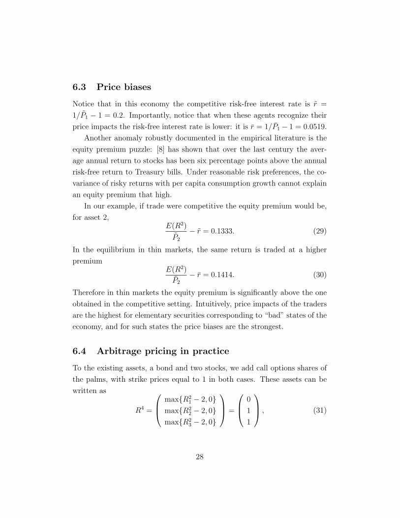
6.4 Arbitrage pricing in practice
To the existing assets, a bond and two stocks, we add call options shares of
the palms, with strike prices equal to 1 in both cases. These assets can be
written as
R4 =
max{R21 − 2, 0}
max{R22 − 2, 0}
max{R23 − 2, 0}
=
0
1
1
, (31)
28
and
R5 =
max{R31 − 2, 0}
max{R32 − 2, 0}
max{R33 − 2, 0}
=
1
0
1
. (32)
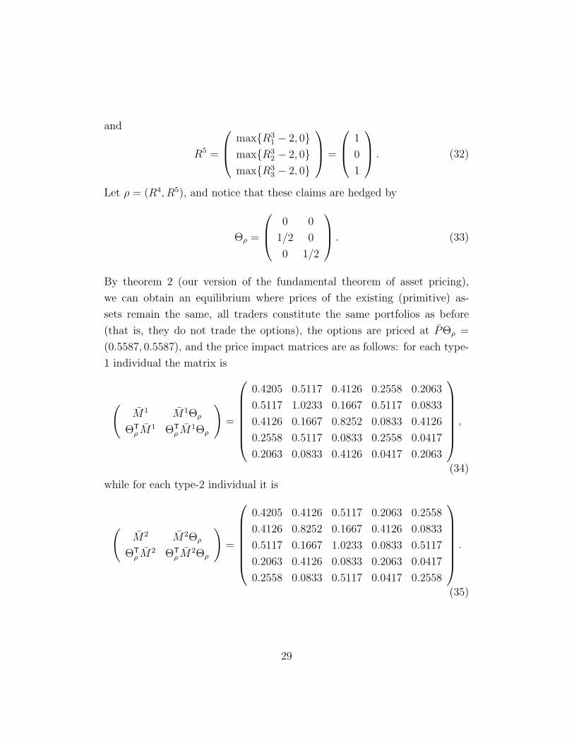
Let ρ = (R4, R5), and notice that these claims are hedged by
Θρ =
0 0
1/2 0
0 1/2
. (33)
By theorem 2 (our version of the fundamental theorem of asset pricing),
we can obtain an equilibrium where prices of the existing (primitive) as-
sets remain the same, all traders constitute the same portfolios as before
(that is, they do not trade the options), the options are priced at PΘρ =
(0.5587, 0.5587), and the price impact matrices are as follows: for each type-
1 individual the matrix is
(M1 M1Θρ
ΘTρ M1 ΘT
ρ M1Θρ
)=
0.4205 0.5117 0.4126 0.2558 0.2063
0.5117 1.0233 0.1667 0.5117 0.0833
0.4126 0.1667 0.8252 0.0833 0.4126
0.2558 0.5117 0.0833 0.2558 0.0417
0.2063 0.0833 0.4126 0.0417 0.2063
,
(34)
while for each type-2 individual it is
(M2 M2Θρ
ΘTρ M2 ΘT
ρ M2Θρ
)=
0.4205 0.4126 0.5117 0.2063 0.2558
0.4126 0.8252 0.1667 0.4126 0.0833
0.5117 0.1667 1.0233 0.0833 0.5117
0.2063 0.4126 0.0833 0.2063 0.0417
0.2558 0.0833 0.5117 0.0417 0.2558
.
(35)
29
7 Concluding remarks
We have studied a model of trade in financial markets where individual in-
vestors recognize the fact that prices do depend on their trades. In this
setting, the argument why asset prices do not allow for arbitrage opportuni-
ties at equilibrium fails. In the customary argument, arbitrage opportunities
cannot exist because if they do, the portfolios that individuals are demanding
cannot be optimal: whatever her preferences and believes20 adding one unit
of the arbitrage opportunity to the existing portfolios of one trader would
make her strictly better-off. Thus, according to this argument, equilibrium
asset prices eliminate arbitrage opportunities and embed, in consequence, an
objective probability distribution that allows to price any state-contingent
claim in the economy as the discounted expected return it entails. This is
the foundation of the theory of asset pricing. But, indeed, this argument is
untenable if one believes that individual investors do anticipate that their
trades will affect asset prices: even if an arbitrage opportunity exists, it may
be that an investor’s attempt to exploit it affects the prices in a way such that
the cost of her existing portfolio increases to the point that she is no longer
better-off in ex-ante terms. If a theory of asset pricing based on an objective
probability embedded in prices is going to be consistent with noncompetitive
behavior of investors, a new argument has to be provided.
In this paper, we have tackled that question in the context of a two-
period, financial economy with a finite number of states of the world. We
have considered a situation in which all traders know that, given a status quo
of prices and trades in the market, if they were to attempt a different trade,
they would (have to) affect prices in order to guarantee that the rest of the
market is willing to accommodate their increased demands or sales. In such a
case, the predictions of models where all traders follow price-taking behavior
are inapplicable. For instance, each individual’s willingness to trade is lower
than in the competitive case, and, consequently, not all gains to trade are
exhausted and trade leads to an equilibrium in which the asset allocation
is Pareto-inefficient.21 Here, we have shown that, even in noncompetitive
30
financial markets, financial equilibria that preclude arbitrage opportunities
do exist.
Some assumptions were made. Firstly, we only consider agents with pref-
erences that have von Neumann-Morgenstern representation with respect
to future consumption, and that are quasilinear with respect to date-zero
consumption, a variable in which we impose no non-negativity constraints;
effectively, these assumptions leave all future consumption free of income
effects, and simplifies substitution effects across consumption in different
states of the world, which makes our mathematical problem more tractable.
Secondly, we consider only the case in which the existing financial markets
allow for complete insurance opportunities against risk; this allows us to ob-
tain an auxiliary representation of the economy by replacing the financial
markets with a complete set of elementary securities, in which, thanks to
the separability of preferences, we can restrict attention to the case when
price cross-effects are null: each agent beliefs, a posteriori correctly, that
if she expands her order for some security, only the price of that security
will be affected. We then invoke the argument of [14] to prove the existence
of equilibria in the auxiliary economy in which no arbitrage opportunities
can exist. Critically, though, this conclusion follows as a consequence of the
facts that all traders are individually rational and all markets are clearing,
which contrasts with the competitive case, in which the existence of just one
individually rational trader suffices for the conclusion, regardless of market
clearing. We then associate the equilibria of the auxiliary economy with
equilibria on the original financial structure, and obtain that at these equi-
libria no arbitrage opportunities can exist either. Furthermore, we provide
an extension of the fundamental theorem of asset pricing to (two-period, fi-
nite) noncompetitive economies, which allow not only for the computation
of the prices of redundant securities, but also for the direct determination of
the price impacts exerted by these securities (and also of those exerted by
other securities on these). The effect of market thinness on asset prices is
not clear without further assumptions. If one assumes a symmetric economy
31

with CRRA preferences, asset prices are above the ones that would prevail
were the markets competitive.22
Critically, in our analysis market power is determined endogenously, as
part of the definition of equilibrium. Here, we have considered the case in
which traders correctly estimate their price impacts to a first-order level
of accuracy: implicit in their individual portfolio problems, they impute a
correct linear approximation to the real inverse demand they face from the
rest of the market (which, in itself, depends on the estimations other traders
are making of the inverse demand they face, which depend on the estimation
made by the trader in question). This assumption simplifies the definition
and treatment of equilibrium, in that it guarantees that each trader’s solution
to her portfolio problem is characterized by its first-order conditions, but is
of no further importance. Moreover, [15] provides strategic foundations for
the equilibrium used here.
The extension of these results, and the relaxation of the assumptions
made here remain topics for further research. If one guarantees that the
second-order conditions of the portfolio problem are satisfied for each trader,
then the assumption that they only estimate their inverse demands to a first-
order level of accuracy can be removed. The assumptions of separability and
quasilinearity are useful, but ought to be relaxed. Most critically, however,
the question of whether our results hold true for economies with incomplete
financial markets remains open.
32
Appendix A1: lemmata
Proof of lemma 1: For necessity, the first two conditions are immediate, andwe only need to concentrate on the third condition.
For any investor j, since Θj is stable given (P , M j) it must be that itsolves the equation P = RT∂uj(ej + RΘj) − M jΘj. By strong concavityof preferences, nonredundancy of assets and positive definiteness of the priceimpact matrix, this defines, locally around P , a differentiable individual (sta-ble) demand function Θj(P ; M j), with derivative
∂P Θj(P ; M j) = (RT∂2uj(ej + RΘj)R− M j)−1, (36)
a negative definite matrix.Thus, the demand trader i faces from the rest of the market is, locally
around P , ϕi(P ) =∑
j 6=i Θj(P ; M j). By construction,
∂ϕi(P ) =∑j 6=i
(RT∂2uj(ej + RΘj)R− M j)−1, (37)
again a negative definite matrix. A subequilibrium triggered by a local devi-ation Θi (close enough to Θi) requires prices P such that ϕi(P ) = −Θi. Thisdefines, locally, a differentiable subequilibrium price function φi(Θi), withthe property that
∂φi(Θi) = −(∂ϕi(P ))−1 = H((M j −RT∂2uj(ej + RΘj)R)j 6=i). (38)
Now, since M is mutually consistent given (P , Θ), there exists a localinverse demand function P i. Since subequilibria are locally unique, it must bethat, in a neighborhood of Θi, φi(Θi) = P i(Θi), which immediately implies,again by mutual consistency of M , that
M i = ∂P i(Θi) = ∂φi(Θi) = H((M j −RT∂2uj(ej + RΘj)R)j 6=i). (39)
For sufficiency, market clearing and stability of all trades are immediate,and we only need to prove mutual consistency of profile M .
As in the proof of necessity, by the second condition of the lemma, foreach trader i we again have, locally around P , an inverse demand function
33
ϕi(P ) =∑
j 6=i Θj(P ; M j), with
∂ϕi(P ) =∑j 6=i
(RT∂2uj(ej + RΘj)R− M j)−1 (40)
a negative definite matrix. By the implicit function theorem we can findneighborhoods N i(Θi) and N i(P ), and a diffeomorphism ρi : N i(Θi) →N i(P ), such that
a. P i(Θi) is the only P in N i(P ) satisfying that ϕi(P ) + Θi = 0;
b. ∂P i(Θi) = −(∑
j 6=i(RT∂2uj(ej + RΘj)R− M j)−1)−1.
By property (a), for every Θi ∈ N(Θi), P i(Θi; M−i) ∩ N(P ) = {P i(θi)},while, by property (b) and the third condition of the lemma, ∂P i(Θi) =M i.
Proof of lemma 3: That prices in the set allow no weak arbitrage opportuni-ties is straightforward. Now, vector P allows no weak arbitrage opportunitiesif, and only if, there exists no solution to the system
P ·Θ < 0, RΘ = 0. (41)
It follows from Farkas’s lemma that if P allows no weak arbitrage opportuni-ties, then for some (p0, p1) ∈ R++ × RS, it is true that p0P = RTp1. Lettingp = 1
p0p1 completes the proof.
Proof of lemma 4: Write
M =
(MS ∆∆T Γ
). (42)
Define
T =
(−R−1
S RA−S
IA−S
), (43)
and notice that RT = 0. Since M gives no irrelevant impact, it follows thatMT = 0, which implies that MSR−1
S RA−S = ∆ and ∆TR−1S RA−S = Γ.
Now, by direct computation,
RTmR =
(MS RT
SmRA−S
RTA−SmRS RT
A−SmRA−S
), (44)
34
whereas RTmRT = 0, so MSR−1S RA−S = RT
SmRA−S. Immediately, it followsthat RT
SmRA−S = ∆, which implies that RTA−SmRA−S = ∆TR−1
S RA−S = Γ,and hence that RTmR = M .
For uniqueness, suppose that RTmR = M . Then,
m = (RTS)−1RT
SmRS(RS)−1 = (RTS)−1MS(RS)−1 = m. (45)
Proof of lemma 5. By construction,∑j 6=i
(Θj + (I − 1)−1(Θi − Θi)) + Θi =∑j 6=i
Θj + Θi − Θi + Θi = 0, (46)
and hence all markets clear. It only remains to show that for each j 6= i,trade Θj +(I − 1)−1(Θi− Θi) is stable for j given (P , M j). Suppose not: forsome j and some Θj,
U j(−(P + M j(Θj − (Θj + (I − 1)−1(Θi − Θi)))) ·Θj, ej + RΘj)
> U j(−P · (Θj + (I − 1)−1(Θi − Θi)), ej + R(Θj + (I − 1)−1(Θi − Θi))).
Since R(Θi− Θi) = 0 and M j gives no irrelevant price impact, it follows thatM j(Θi−Θi) = 0 and, by proposition 1, P ·(Θi−Θi) = 0. Then, the previousequation is equivalent to
U j(−(P + M j(Θj − Θj)) ·Θj, ej + RΘj) > U j(−P · Θj, ej + RΘj), (47)
which means that Θj is not stable for j given (P , M j), contradicting the factthat (P , Θ−i) is a subequilibrium triggered by trade Θi.
Proof of lemma 6. For notational definiteness, we denote by S i(Θi; M−i, R)and P i(Θi; M−i, R) the sets of subequilibria triggered by Θi, given M−i,and its projection into the space of prices, when the economy is endowedwith asset structure R. We distinguish these sets for the case of elementarysecurities, by denoting them as S i(Θi; M−i, IS) and P i(Θi; M−i, IS).
Notice first that, since each (M i, mi) is R-associated, it is immediatethat all M i give no irrelevant price impacts. Also, notice that, by lemma 4,mi = (R−1
S )TM iSR−1
S for all i.For the first claim, suppose that (p, θ, m) is an equilibrium for {U, e, IS}
and∑
i Θi = 0. Market clearing is assumed, so we only need to show that
35
each Θi is stable for i given (P , M i), and that the profile M is mutuallyconsistent.
Suppose that Θi is not stable for i given (P , M i). Then, we can fix Θsuch that
−(P + M i(Θ− Θi)) ·Θ + ui(ei + RΘ) > −P · Θi + ui(ei + RΘi). (48)
Given that (P , Θ, M) and (p, θ, m) are R-associated, it follows that
−(RTp+RTmiR(Θ−Θi))·Θ+ui(ei+RΘ) > −(RTp)·Θi+ui(ei+RΘi), (49)
so, letting θ = RΘ, by direct computation,
−(p + mi(θ − θi)) · θ + ui(ei + θ) > −p · θi + ui(ei + θi), (50)
contradicting the fact that, in the economy with elementary securities, θi isstable for i given (p, mi).
Now, for each i, by mutual consistency of profile m, there exist neighbor-hoods N i(θi) and N i(p) and a differentiable, local inverse demand functionpi : N i(θi) → N i(p) such that pi(θi) = p and ∂pi(θi) = mi. Then, we candefine open neighborhoods
N i(Θi) = {Θ|RΘ ∈ N i(θi)} (51)
andN i(P ) = {P |(RT
S)−1(P1, . . . , PS)T ∈ N i(p)}. (52)
By construction,f(Θ) = RΘ maps N i(Θi) into N i(θi), and g(p) = RTp mapsN i(p) into N i(P ), so we can define P i = g ◦ pi ◦ f : N i(Θi) → N i(P ). First,notice that P i(Θi) = RTpi(RΘi) = RTp = P , while
∂P i(Θi) = RT∂pi(θi)R = RTmiR = M i. (53)
We now want to show that for any Θ ∈ N i(Θi), P i(Θ) is the unique (lo-cally) subequilibrium price triggered by Θi = Θ, namely that P i(Θ; M i, R)∩N i(P ) = {P i(Θ)}. First, notice that in the economy with elementary secu-rities, for some θ−i, (pi(RΘ), θ−i) ∈ S i(RΘ; m−i, IS). Defining
Θj =
(R−1
S (θj + 1I−1
RΘ)
0
)− 1
I − 1Θ, (54)
36
for each j 6= i, it follows that (P i(Θ), (Θj)j 6=i) ∈ S i(Θ; M i, R), and hencethat P i(Θ) ∈ P i(Θi; M−i, R). Now, suppose that there exists another P ∈P i(Θ; M−i, R) ∩ N i(P ). Then, for some Θ−i, (P, Θ−i) ∈ S i(Θ; M−i, R).Since each M j gives no irrelevant price impact, it follows from proposition1 that P allows no weak arbitrage opportunities, and then, from lemma3, that there exists p ∈ RS such that RTp = P . By construction, p =(RT
S)−1(P1, . . . , PS)T ∈ N i(p) and
((RTS)−1P, (RΘj)j 6=i) ∈ S i(RΘ; m−i, IS). (55)
Also by construction, p 6= pi(RΘ) and p ∈ N i(p) ∩ P i(RΘ; m−i, IS), whichis impossible. It follows that for each i, P i : N i(Θi) → N i(P ) is a (differen-tiable) local inverse demand: for all Θ ∈ N i(Θi),
P i(Θ; M−i, R) ∩N i(P ) = {P i(Θ)}; (56)
since ∂P i(Θi) = M i, it follows that M is mutually consistent.For the second claim, suppose that (P , Θ, M) is an equilibrium for {U, e, R}.
Market clearing is immediate:∑
i θi =
∑i RΘi = R
∑i Θ
i = 0. As before,we now show that each θi is stable for i given (p, mi), and that m is mutuallyconsistent.
Suppose that θi is not stable for i given (p, mi). Then, we can fix θ suchthat
−(p + mi(θ − θi)) · θ + ui(ei + θ) > −p · θi + ui(ei + θi). (57)
Fix any Θ such that RΘ = θ. Given that (P , Θ, M) and (p, θ, m) are R-associated, it follows by direct computation that
−(P + M i(Θ− Θi)) ·Θ + ui(ei + RΘ) > −P · Θi + ui(ei + RΘi). (58)
contradicting the fact that, in the economy with market R, Θi is stable for igiven (P , M i).
Now, for each i, by mutual consistency of profile M , there exist neigh-borhoods N i(Θi) and N i(P ) and a differentiable local subequilibrium pricefunction P i : N i(Θi) → N i(P ) such that P i(Θi) = P and ∂P i(Θi) = M i.Then, we can define open neighborhoods
N i(θi) =
{θ|(
R−1S (θ − θi)
0
)+ Θi ∈ N i(Θi)
}(59)
37
andN i(p) = {p|RTp ∈ N i(P )}. (60)
By construction
F (θ) =
(R−1
S (θ − θi)0
)+ Θi (61)
maps N i(θi) into N i(Θi), and G(P ) = (RTS)−1(P1, . . . , PS)T maps N i(P ) into
N i(p), so we can define pi = G ◦ P i ◦ F : N i(θi) → N i(p). Notice thatpi(θi) = (RT
S)−1P i(Θi) = p, while
∂pi(θi) =(
(R−1S )T 0
)∂P i(Θi)
(R−1
S
0
)= (R−1
S )TM iSR−1
S = mi. (62)
It only remains to show that for any θ ∈ N i(θi), P i(Θ; M i, IS)∩N i(p) ={pi(θ)}. Let Θ = F (θ). Notice that in the economy with market R, forsome Θ−i, (P i(Θ), Θ−i) ∈ S i(Θ; M−i, R). Defining, for each j 6= i, θj =RΘj, it follows that (pi(θ), (θj)j 6=i) ∈ S i(θ; mi, IS), and hence that pi(θ) ∈P i(θ; mi, IS). Now, suppose that there exists another p ∈ P i(θ; mi, IS) ∩N i(p). Then, for some θ−i, (p, θ−i) ∈ S i(θ; mi, IS). By construction, P =RTp ∈ N i(P ) and (RTp, (R−1
S θj, 0)j 6=i) ∈ S i((R−1S θ, 0); M−i, R). By lemma
5,
P i
(((RS)−1θ
0
); M−i, R
)= P i(Θ; M−i, R), (63)
so RTp ∈ P i(Θ; M−i, R). As before, by construction, P 6= P i(Θ) and P ∈N i(P ) ∩ P i(Θ; M−i, R), which is impossible.
Appendix A2: existence and generic determi-
nacy of equilibria in elementary securities
Existence
We now specialize the proof of theorem 1 in [14], for the particular casetreated here. All the arguments in this appendix are given for an economywith elementary securities, {U, e, IS} satisfying our assumptions about pref-erences and endowments. Since we will only consider positive definite anddiagonal price impact matrices, we identify these matrices with vectors inRS
++.
38
Let h : (RS+, RS
++)I−1 → RS++ be the (component-wise) harmonic mean
(divided by (I − 1)); that is,
hs(m, v) = (∑
j
(mjs + vj
s)−1)−1. (64)
Function h is continuous, and it is well known that
(I − 1)hs(m, v) ≤ (I − 1)−1∑
j
(mjs + vj
s), (65)
for all m, all v and all s.
Claim 1. Let γu be any strictly positive number, and let (m, v) ∈ (RS+, RS
++)I−1.Suppose that for some s, mj
s ≤ (I − 2)−1γu and vjs ≤ γu for all j. Then,
hs(m, v) ≤ (I − 2)−1γu.
Proof. This is immediate, since
(I − 1)hs(m, v) ≤∑
j mjs
I − 1+
∑j vj
s
I − 1≤ γu
I − 2+ γu. (66)
Define, for each state s, µs = maxi{∂uis(e
is)}, a strictly positive real
number. By the Inada conditions, we can fix, for each trader i and state s,a revenue transfer θi
s such that ∂uis(e
is + θi
s) = µs. By concavity and Inada,−ei
s < θis ≤ 0.
Construct the (truncation) set of trades
T = {θ ∈ (RS)I :∑
i
θis = 0 and θi
s ≥1
2(θi
s − eis) for all i and all s}, (67)
which is nonempty, convex and compact.Define the function V : T → (RS
++)I , componentwise, by letting V is (θ) =
−∂2uis(e
is + θi
s).23 Since T is compact, V is continuous and I and S are
finite, we can further define real numbers γu = maxθ∈T maxi,s V is (θ) and
γd = minθ∈T mini,s V is (θ); these numbers, by construction, satisfy that 0 <
γd ≤ γu.
39

Define the function U : ([0, (I − 2)−1γu]S)I → (RS)I by
U(m) = arg maxθ∈T
∑i,s
(uis(e
is + θi
s)−1
2mi
s(θis)
2), (68)
which is well defined since T is compact and convex, each ui is continuous andstrongly concave, and each mi
s ≥ 0. Define also the function H : ([γd, γu]S)I×
([0, (I − 2)−1γu]S)I → (RS)I , by letting H i(m, v) = h(m−i, v−i).
Finally, define the function F : T × ([γd, γu]S)I , ([0, (I − 2)−1γu]
S)I →(RS)I × (RS)I × (RS)I , by
F(θ, v, m) =
U(m)V (θ)
H(m, v)
. (69)
Claim 2. There exists (θ, v, m) ∈ T × ([γd, γu]S)I × ([0, (I − 2)−1γu]
S)I suchthat F(θ, v, m) = (θ, v, m).
Proof. By construction, U maps into T , and V into ([γd, γu]S)I . By claim
1, H maps into ([0, (I − 2)−1γu]S)I . It follows that F maps a convex and
compact set continuously into itself, so it has a fixed point.
Let a fixed point, (θ, v, m), of F be fixed.
Claim 3. For all i and all s, it is true that θis > 1
2(θi
s − eis).
Proof. Suppose not: suppose that for some i and some s, θis = 1
2(θi
s − eis).
Since θis ≤ 0, it follows that θi
s < 0, which implies that, for some j 6= i,θj
s > 0. By the definition of function U , it follows, then, that
∂uis(e
is + θi
s)− misθ
is ≤ ∂uj
s(ejs + θj
s)− mjsθ
js, (70)
which is impossible, since
∂uis(e
is + θi
s)− misθ
is = ∂ui
s(1
2(ei
s + θis))− mi
sθis > µs, (71)
whereas∂uj
s(ejs + θj
s)− mjsθ
js < ∂uj
s(ejs) ≤ µs. (72)
40
We can now conclude that given preferences and endowments {U, e}, thereexists an equilibrium in elementary securities (p, θ, m) satisfying that all priceimpact matrices are diagonal.
To see this, notice that, given concavity of all preferences and since mis ≥ 0
for all i and all s, it follows from claim 3 that θ actually solves program
maxθ:
∑i θi=0
∑i,s
(uis(e
is + θi
s)−1
2mi
s(θis)
2). (73)
The first-order conditions of this problem immediately imply that there existLagrange multiplies p ∈ RS such that, for all i and all s,
∂uis(e
is + θi
s)− misθ
is = ps. (74)
Identifying mi and vi with the diagonal, positive definite matrices mi1 . . . 0
.... . .
...0 . . . mi
S
and
vi1 . . . 0...
. . ....
0 . . . viS
, (75)
respectively, we get that:
1.∑
i θi = 0;
2. for each trader i, ∂ui(ei + θi)− miθi = p;
3. for each trader i, mi = (I − 1)−1H(m−i + v−i)
4. for each trader i, vi = −∂2ui(ei + θi).
Then, it is immediate from lemma 1 that (p, θ, m) is an equilibrium.
Generic determinacy
Assume now that, moreover, each Bernoulli function uis is of class C3 and
satisfies that ∂2uis is bounded strictly below zero.
Denote by U the class of Bernoulli functions that satisfy all the assump-tions we have imposed,24 and endow this set with the topology of C3 uniformconvergence on compacta.25 The space of economies we now consider is theset (RS
++)I × (US)I , endowed with the product topology.
41
We want to show that, in a dense subset of these economies, all equilibriain elementary securities are locally unique.
To do this, fix an economy {U , e} and an open neighborhood O of thateconomy. We need to show that for at least one economy {U, e} in O theproperty of local uniqueness holds true.
A finite-dimensional subspace of economies
As the space of economies is an infinite dimensional manifold, it is convenientto do our analysis in a finite-dimensional, local subspace of economies. Thestrategy is to show that in this subspace we can find the economy {U, e},where local uniqueness holds, arbitrarily close to {U , e}. In this section, wedefine the subspace of economies.
Fix ε > 0, and a C∞ function ρ : R++ → R+ such that
ρ(x) =
{1, if x < maxs{
∑i e
is}+ Iε + 1;
0, if x ≥ maxs{∑
i eis}+ Iε + 2.
(76)
Also, define for each i and s the “perturbed Bernoulli” function uis : R++ ×
R → R by
uis(x
is, δ
is) = ui
s(xis) +
1
2ρ(xi
s)δis(x
is)
2.
Since each maxs{∑
i eis} is finite, there exists δ > 0 such that for all −δ <
δis < δ, function ui
s(·, δis) ∈ U.
Now, we consider the finite dimensional subset of economies defined byendowments e ∈ Bε(e), and preferences given, for each i and s, by ui
s(·, δis) for
some δis ∈ Bδ(0). This is a submanifold parameterized by Bε(e) × Bδ(0)
SI .For notational simplicity, we identify the vector δi = (δi
s)s with the diagonalmatrix diag(δi
s), and denote δ = (δi)i. Similarly, we again identify the vectormi = (mi
s)s with the diagonal matrix diag(mis).
42
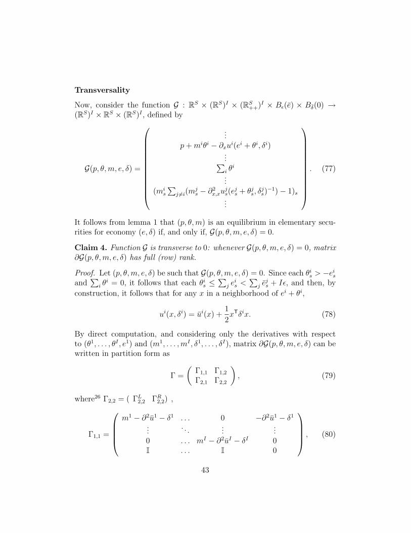
Transversality
Now, consider the function G : RS × (RS)I × (RS++)I × Bε(e) × Bδ(0) →
(RS)I × RS × (RS)I , defined by
G(p, θ,m, e, δ) =
...p + miθi − ∂xu
i(ei + θi, δi)...∑i θ
i
...(mi
s
∑j 6=i(m
js − ∂2
x,xujs(e
js + θj
s, δjs)−1)− 1)s
...
. (77)
It follows from lemma 1 that (p, θ,m) is an equilibrium in elementary secu-rities for economy (e, δ) if, and only if, G(p, θ,m, e, δ) = 0.
Claim 4. Function G is transverse to 0: whenever G(p, θ,m, e, δ) = 0, matrix∂G(p, θ,m, e, δ) has full (row) rank.
Proof. Let (p, θ,m, e, δ) be such that G(p, θ,m, e, δ) = 0. Since each θis > −ei
s
and∑
i θi = 0, it follows that each θi
s ≤∑
j eis <
∑j ej
s + Iε, and then, by
construction, it follows that for any x in a neighborhood of ei + θi,
ui(x, δi) = ui(x) +1
2xTδix. (78)
By direct computation, and considering only the derivatives with respectto (θ1, . . . , θI , e1) and (m1, . . . ,mI , δ1, . . . , δI), matrix ∂G(p, θ,m, e, δ) can bewritten in partition form as
Γ =
(Γ1,1 Γ1,2
Γ2,1 Γ2,2
), (79)
where26 Γ2,2 = ( ΓL2,2 ΓR
2,2) ,
Γ1,1 =
m1 − ∂2u1 − δ1 . . . 0 −∂2u1 − δ1
.... . .
......
0 . . . mI − ∂2uI − δI 0I . . . I 0
, (80)
43
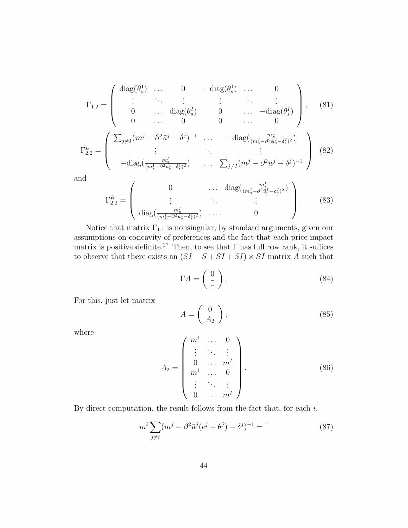
Γ1,2 =
diag(θ1
s) . . . 0 −diag(θ1s) . . . 0
.... . .
......
. . ....
0 . . . diag(θIs) 0 . . . −diag(θI
s)0 . . . 0 0 . . . 0
, (81)
ΓL2,2 =
∑
j 6=1(mj − ∂2uj − δj)−1 . . . −diag( m1
s
(mIs−∂2uI
s−δIs )2
)...
. . ....
−diag( mIs
(m1s−∂2u1
s−δ1s)2
) . . .∑
j 6=I(mj − ∂2uj − δj)−1
(82)
and
ΓR2,2 =
0 . . . diag( m1
s
(mIs−∂2uI
s−δIs )2
)...
. . ....
diag( mIs
(m1s−∂2u1
s−δ1s)2
) . . . 0
. (83)
Notice that matrix Γ1,1 is nonsingular, by standard arguments, given ourassumptions on concavity of preferences and the fact that each price impactmatrix is positive definite.27 Then, to see that Γ has full row rank, it sufficesto observe that there exists an (SI + S + SI + SI)× SI matrix A such that
ΓA =
(0I
). (84)
For this, just let matrix
A =
(0A2
), (85)
where
A2 =
m1 . . . 0...
. . ....
0 . . . mI
m1 . . . 0...
. . ....
0 . . . mI
. (86)
By direct computation, the result follows from the fact that, for each i,
mi∑j 6=i
(mj − ∂2uj(ej + θj)− δj)−1 = I (87)
44
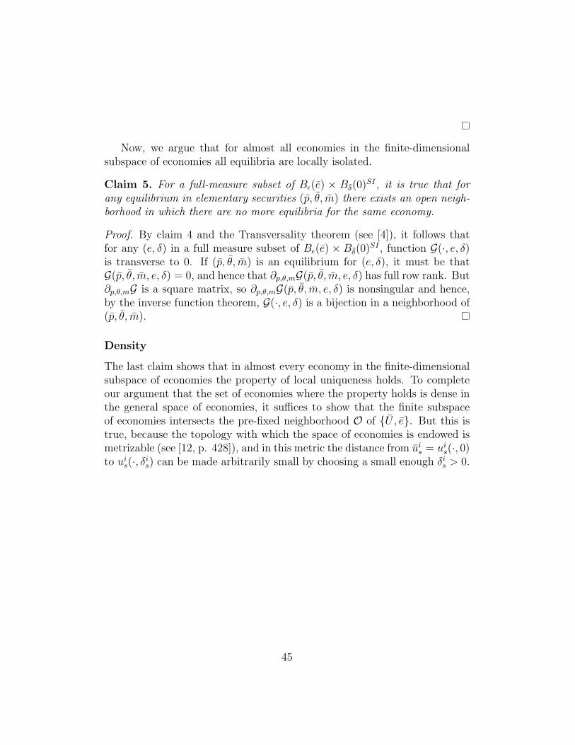
Now, we argue that for almost all economies in the finite-dimensionalsubspace of economies all equilibria are locally isolated.
Claim 5. For a full-measure subset of Bε(e) × Bδ(0)SI , it is true that for
any equilibrium in elementary securities (p, θ, m) there exists an open neigh-borhood in which there are no more equilibria for the same economy.
Proof. By claim 4 and the Transversality theorem (see [4]), it follows thatfor any (e, δ) in a full measure subset of Bε(e) × Bδ(0)
SI , function G(·, e, δ)is transverse to 0. If (p, θ, m) is an equilibrium for (e, δ), it must be thatG(p, θ, m, e, δ) = 0, and hence that ∂p,θ,mG(p, θ, m, e, δ) has full row rank. But∂p,θ,mG is a square matrix, so ∂p,θ,mG(p, θ, m, e, δ) is nonsingular and hence,by the inverse function theorem, G(·, e, δ) is a bijection in a neighborhood of(p, θ, m).
Density
The last claim shows that in almost every economy in the finite-dimensionalsubspace of economies the property of local uniqueness holds. To completeour argument that the set of economies where the property holds is dense inthe general space of economies, it suffices to show that the finite subspaceof economies intersects the pre-fixed neighborhood O of {U , e}. But this istrue, because the topology with which the space of economies is endowed ismetrizable (see [12, p. 428]), and in this metric the distance from ui
s = uis(·, 0)
to uis(·, δi
s) can be made arbitrarily small by choosing a small enough δis > 0.
45
Notes
1 For literature on this, see [10].2 For a review of this literature, see [5].3 The most prominent examples of models include Kyle [7], Vayanos [11].4 This is the feature that closes the definition of equilibrium imposing interesting struc-
ture.5 If we denote by In the n× n identity matrix, then R = IS is the case of a full set of
elementary securities.6 That is, at all c > 0, u′(c) > 0 and u′′(c) < 0, and limc→0 u′(c) = ∞ and
limc→∞ u′(c) = 0.7 The choice of the term “stable” perhaps deserves an explanation. Suppose that trader
i is faced with the following inverse demand function:
p(Θ) = P + M i(Θ− Θ) ·Θ, (88)
where Θ is some reference point. For each Θ, let
Γi(Θ) = arg maxΘ
U i(−(P + M i(Θ− Θ)) ·Θ, ei + RΘ). (89)
The stability condition requires that Θi be a fixed point of this mapping.8 The approximation assures that in the definition of stability the second order condition
is always satisfied. Otherwise, the approximation is without loss of generality.9 Strictly speaking, the intuition given before the definition is slightly weaker than
the definition itself: we do not require that subequilibrium prices be unique (i.e., thatPi(Θi;M−i) be single-valued), but only that they be determinate, or locally unique.
10 So that A = S and RS = R.11 For this result, one also needs to assume the condition of no irrelevant impact, defined
in the following section.12 The no irrelevant impact condition in spirit is similar to a dichotomy between a
monetary and real sector in a standard general equilibrium framework - a consequence ofno money illusion by all agents.
13 The sense in which this result holds for a “typical economy” is established in detailin the proof.
14 That is, the fact that prices P should allow no-arbitrage opportunities.15 Notice that Θρ is an A× A matrix, and not just a column vector. The a-th column
in this matrix is the hedge of the a-th payoff vector in ρ. These portfolios only use thefirst S assets nontrivially.
46
16 Namely, if for all i,
uis(c
is) =
(cis)
1−φs
1− φs, (90)
where φs > 0 is the coefficient of risk aversion (it is well known that in the case φs = 1 onehas that ui
s(cis) = ln(ci
s)). For the result below, the coefficient of risk aversion can changeacross states, but is the same for all individuals, given a state.
17 The third derivative of a CRRA utility function is positive, which implies that ineach state a marginal utility is convex.
18 Till now the only dynamic model of thin trading proposed in [18] assumes quadraticutility functions. The considered return biases require convex marginal utility.
19 This equilibrium can be compared with the competitive equilibrium of this economyin the case of a full set or elementary securities: prices would be p = (1/3, 1/3, 1/6)T,type-1 individuals would buy θ1 = (1,−1, 0)T, which would be sold by type-2 individuals.
20 Assuming, of course, monotonicity of ex-ante preferences on consumption in all futurestates of the world.
21 As long as a priori there are some gains to trade, i.e. the initial endowments arePareto inefficient. The deadweight loss due to non-competitive trading depends negativelyon the depth of the market, and it vanishes completely as a number of traders approachesinfinity (see [14]).
22 For the detailed study of model predictions for different market structures and utilityfunctions, see [14].
23 This function is well defined, since, by construction, θis−ei
s
2 > −eis, so ei
s + θis > 0.
24 Namely, that each uis is differentiably strictly monotonic and differentiably strictly
concave, and satisfies Inada conditions. Unlike in Proposition 5, we do not require nowthat these functions be CRRA.
25 See [1].26 The precise form of matrix Γ2,1 is immaterial for computations below.27 To see this, the argument is the one that gives determinacy in competitive models:
(i) notice that the submatrix composed by the first I superrows and I supercolumns isnonsingular, since it is a diagonal matrix of positive numbers: each mi
s > 0 and each∂2ui
s(eis + θi
s)+ δis < 0, as ui
s(·, δis) is strongly concave; (ii) Now, to see that the whole Γ1,1
is nonsingular, it suffices to observe that if one constructs the S(I + 1) × S matrix A byletting the first S×S superrow be I, letting the last S×S superrow be −(∂2u1(ei + θi) +δ1)−1(m1−∂2u1−δ1), and letting every other element be 0, we get, by direct computation,that
Γ1,1A =
(0I
). (91)
47
References
[1] Aliprantis, C. and Border, K., Infinite Dimensional Analysis, Springer,
1999.
[2] Chan, K.C. and Lakonishok, J., “The behavior of stock price around
institutional trades,” Journal of Finance 50, 1147-1174, 1995.
[3] Gompers, P. and Metrick, A., “Institutional investors and equity prices,”
Quarterly Journal of Economics 116, 1, 229-259, 2001.
[4] Guillemin, V. and A. Pollack, Differential Topology, Prentice Hall, 1974.
[5] Hart, O. “Imperfect competition in general equilibrium: an overview
of recent work,” in Arrow K. and Honkapohja S. (Eds.) Frontiers of
Economics, Blackwell, 1985.
[6] Keim, D. and Madhavan, A., “The upstairs market for large-block trans-
actions: analysis and measurement of price effects,” Review of Financial
Studies 9, 1-39, 1996.
[7] Kyle, A. “Informed Speculation and Imperfect Competition” Review of
Economic Studies 56, 317-356, 1989.
[8] Mera, R. and Prescott, E., “The Equity Premium: A Puzzle,” Journal
of Monetary Economics 15(2), 145-61, 1985.
[9] Negishi, T. “Monopolistic competition and general equilibrium,” Review
of Economic Studies 28, 196-201, 1961.
[10] Perold, A. “The implementation shortfall: papers versus reality,” Jour-
nal of Portfolio Management 14, 3, 1988.
[11] Vayanos, D. “Strategic Trading and Welfare in a Dynamic Market” Re-
view of Economic Studies 66, 219-254, 1999.
48
[12] Villanacci, A., L. Carosi, P. Benevieri and A. Battinelli, Differential
Topology and General Equilibrium with Complete and Incomplete Mar-
kets, Kluwer, 2002.
[13] Weil, P. “The Equity Premium Puzzle and the Risk-Free Rate Puzzle,”
Journal of Monetary Economics, 24(2), 401-21, 1989
[14] Weretka, M. “Endogenous Market Power,” Mimeo, 2005, available from
http://www.ssc.wisc.edu/ mweretka/Research.
[15] Weretka, M. “Discovery of Market Power in Bi-
lateral Oligopoly,” Mimeo, 2007, available from
http://www.ssc.wisc.edu/ mweretka/Research.
[16] Weretka, M. “Cross-Market Effects in Thin Markets,” Mimeo, 2007,
available from http://www.ssc.wisc.edu/ mweretka/Research.
[17] Weretka, M. “Asset Valuation in Thin Financial Markets,” Mimeo, 2007,
available from http://www.ssc.wisc.edu/ mweretka/Research.
[18] Rostek, M. and Weretka, M. “Term structure of Price Impact,” Mimeo,
2007, available from http://www.ssc.wisc.edu/ mweretka/Research.
49


![Asymptotic arbitrage in large financial marketskramkov/publications/FS_98.pdf · arbitrage it has attracted considerable attention, see, e.g., [4], [5], [12], [13], and was extended](https://img.pdfslide.us/doc/110x75/5f6ea2283d7615180353a8f7/asymptotic-arbitrage-in-large-inancial-kramkovpublicationsfs98pdf-arbitrage.jpg)

![Weak and strong no-arbitrage conditions for continuous ...1302.7192v2 [q-fin.PR] 14 May 2014 Weak and strong no-arbitrage conditions for continuous financial markets Claudio Fontana](https://img.pdfslide.us/doc/110x75/5ae5bf397f8b9a87048d051f/weak-and-strong-no-arbitrage-conditions-for-continuous-13027192v2-q-finpr.jpg)