Discussion Papers in Economics

Department of Economics and Related Studies

University of York

Heslington

York, YO10 5DD

No. 19/18

Predicting interest rates in real-time

Alberto Caruso, Laura Coroneo

Predicting interest rates in real-time

Alberto Caruso∗

ConfindustriaECARES, Universite Libre de Bruxelles

Laura Coroneo†

University of York

November 28, 2019

Abstract

We analyse the predictive ability of real-time macroeconomic information for theyield curve of interest rates. We specify a mixed-frequency macro-yields modelin real-time that incorporates interest rate surveys and that treats macroe-conomic factors as unobservable components. Results indicate that real-timemacroeconomic information is helpful to predict interest rates, and that datarevisions drive a superior predictive ability of revised macro data over real-timemacro data. Moreover, we find that incorporating interest rate surveys in themodel can significantly improve its predictive ability.

JEL classification codes: C33, C53, E43, E44, G12.Keywords: Government Bonds; Dynamic Factor Models; Real-time Forecasting; Mixed-frequencies.

∗Contact: Confindustria, Viale dell’Astronomia 30, 00144 Roma, Italy. Email: al-berto.caruso01@gmail.com. Web: www.alberto-caruso.com†Contact: Department of Economics and Related Studies, University of York, Hes-

lington, YO10 5DD York, United Kingdom. Email: laura.coroneo@york.ac.uk. Web:www.sites.google.com/view/lauracoroneo.

We thank Carlo Altavilla, Domenico Giannone, Ivan Petrella, Lucrezia Reichlin, and seminar andconference participants at the University of York, the 2nd conference on Forecasting at Central Banks(Bank of England), the NBP Workshop on Forecasting (Bank of Poland), the Workshop on Big Data andEconomic Forecasting (European Commission), the 8th Italian Congress of Econometrics and EmpiricalEconomics (University of Salento), the 12th International Conference on Computational and FinancialEconometrics (University of Pisa), the Annual Conference of the International Association for AppliedEconometrics (IAAE 2019, Nicosia) and the Conference on Real-Time Data Analysis, Methods andApplications (National Bank of Belgium) for useful comments. The authors acknowledge the support ofNow-Casting Economics Ltd. in the early stage of the paper. The views expressed in this paper are thoseof the authors and do not necessarily reflect those of Confindustria.

1

1 Introduction

Macroeconomic variables may incorporate important information for forecasting the evo-

lution of the yield curve. This is due to both the behaviour of market agents, who closely

monitor macroeconomic data and react to macroeconomic news, and policy makers, who

operate on interest rates to stimulate aggregate demand and control inflation. Indeed,

following the seminal work by Ang & Piazzesi (2003), there is a consensus in the litera-

ture that macroeconomic indicators are successful at predicting interest rates and excess

bond returns, see among others Monch (2008), Ludvigson & Ng (2009), Favero, Niu & Sala

(2012) and Coroneo, Giannone & Modugno (2016). However, Ghysels, Horan & Moench

(2017) find limited evidence of predictive ability of real-time macroeconomic variables for

excess bond returns: they argue that the result of the previous literature was an artefact

coming from the use of revised data, instead of real-time macroeconomic data.1

In this paper, we assess the relevance of real-time macroeconomic information to predict

the future path of the yield curve of interest rates. Our contribution is to use filtering

techniques to exploit the informative content of real-time macroeconomic data, and to

properly specify the information set available to agents in each point in time by taking

into account all the characteristics of the real-time macroeconomic data flow.2 First, most

macroeconomic data is released in a non-synchronous way and with different publication

lags; therefore the available information at each point in time can be described by a dataset

that has a ragged edge, and it is not balanced. Second, macroeconomic data is very often

subsequently revised: the revisions might be substantial and affect the estimation and the

forecast computed using different vintages of the data. Third, in real-time forecasting, soft

information provided by surveys can have an important role as it is timely, not subject

to revisions and can readily incorporate any information available to survey participants,

such as information about the current state of the economy or forward-looking information

1A common denominator of this literature, in fact, is the use of revised macroeconomic data to predictinterest rates, which involves using an information set that is different from the one available to marketparticipants when the predictions were made.

2Adequately specifying the information set available to agents in real-time is particularly importantwhen evaluating models in macroeconomics and finance, especially when the objective is to forecast assetprices using external information, since according to the efficient market hypothesis asset prices shouldalready incorporate all the available information about their future evolution, see Orphanides (2001),Orphanides & Van Norden (2002) and Croushore & Stark (2003).

2

contained in monetary policy announcements. However, one drawback of using survey

expectations is that they are released only infrequently, most often on a quarterly basis.

In order to study interest rate predictability in real-time while also addressing these

drawbacks, we specify a mixed-frequency macro-yields model in real-time that incorporates

interest rate surveys and treats macroeconomic factors as unobservable components, which

we extract simultaneously with the traditional yield curve factors. Similarly to Coroneo

et al. (2016), we identify the factors driving the yield curve by constraining the loadings

to follow the smooth pattern proposed by Nelson & Siegel (1987). More specifically, our

empirical model is a mixed-frequency dynamic factor model for Treasury zero-coupon yields,

a representative set of real-time macroeconomic variables and interest rate surveys with

restrictions on the factor loadings.

Our model can be estimated by maximum likelihood – see Doz, Giannone & Reichlin

(2012) – using an Expectation-Maximization (EM) algorithm adapted to the presence of

restrictions on the factor loadings and to missing data. Using U.S. data from 1972 to 2016,

we find that real-time macroeconomic information is helpful to predict interest rates, espe-

cially short maturities at mid and long horizons, and that data revisions drive an increase

in the predictive power of revised macro information with respect to real-time macro infor-

mation. Moreover, during a period when a forward guidance policy is implemented, we find

that incorporating interest rate surveys in the model significantly improves its predictive

ability.

Our finding that data revisions drive the increased predictive ability of revised macro

data with respect to real-time macro data is in line with Ghysels et al. (2017). However,

while they find that real-time macro information has only a marginal (and often statistically

non significant) role in predicting excess bond returns, our results show that real-time

macroeconomic information is still helpful to predict interest rates, as its predictive power

is similar to that of revised macro data. Moreover, in contrast to Ghysels et al. (2017),

we find that real-time macro variables have a stronger predictive ability than their first

releases, which is in line with the intuition that revisions of first releases enhance the

quality of macroeconomic information; it is also in line with the macro forecasting literature

that uses the latest available vintage of data (i.e. real-time data) in each point in time,

3

rather than first releases, to nowcast and forecast macro aggregates (Koenig, Dolmas &

Piger 2003, Croushore & Stark 2003). The reason for the superior predictive ability of our

real-time macro-yield model is our use of filtering techniques that allow us to efficiently

extract information from a truly real-time data set with a ragged edge.

Lastly, we find that incorporating interest rate surveys from the Surveys of Professional

Forecasters can improve the predictive ability of models that use only information embedded

in the yield curve and in macroeconomic variables. Surveys, in fact, incorporate soft

information about the future path of interest rates – that comes from policy announcements,

for example – that cannot be taken into account by standard macroeconomic variables.

With this in mind, we test the predictive ability of the model by incorporating surveys in a

period in which the Federal Reserve implemented a forward guidance policy. The resulting

improvement in predictive ability is statistically significant. This intuitively appealing

result is in line with Altavilla, Giacomini & Ragusa (2017), who use the selected survey

forecast value as their forecast for the specific horizon and maturity. However, our results

show that in some periods our model produces more accurate forecasts than the surveys

themselves. Therefore, we incorporate the surveys into the model itself. In this way, we

combine in a single framework the “soft” information embedded in the surveys with the

information carried by interest rates and by the real-time macroeconomic data about the

state of the economy, fully exploiting all the relevant available information in forecasting

the whole yield curve.

The paper is organized as follows. Section 2 outlines the mixed-frequency real-time

macro-yields model. Section 3 describes the data and Section 4 outlines the estimation

procedure and some preliminary results. Section 5 describes the out-of-sample forecasting

exercise, and Section 6 the results. Finally, Section 7 concludes. Appendix A contains

details about the state-space representation of the model and the estimation procedure.

2 Model

We model the joint behavior of monthly government bond yields, real-time macroeconomic

indicators, and quarterly interest rate surveys using a mixed-frequency dynamic factor

model. Bond yields at different maturities are driven by the traditional level, slope and

4

curvature factors, while real-time macroeconomic variables load on the yield curve factors as

well as on some additional macro factors that capture the information in macroeconomic

variables over and above the yield curve factors. Finally, interest rate surveys load on

quarterly averages of the monthly yield and macro factors. In what follows, we describe

each point in detail.

2.1 Yields

We model the cross-section of bond yields using the Dynamic Nelson-Siegel framework of

Diebold & Li (2006). Denoting by yt the Ny×1 vector of yields with Ny different maturities

at time t, we have

yt = ay + Γyy Fyt + vyt , (1)

where F yt is a 3 × 1 vector containing the latent yield-curve factors at time t, Γyy is a

Ny × 3 matrix of factor loadings, and vyt is an Ny × 1 vector of idiosyncratic components.

The yield curve factors F yt are identified by constraining the factor loadings to follow the

smooth pattern proposed by Nelson & Siegel (1987)

ay = 0; Γ(τ)yy =

[1

1− e−λτ

λτ

1− e−λτ

λτ− e−λτ

]≡ Γ

(τ)NS, (2)

where Γ(τ)yy is the row of the matrix of factor loadings corresponding to the yield with

maturity τ months and λ is a decay parameter of the factor loadings. Diebold & Li (2006)

show that this functional form of the factor loadings implies that the three yield curve

factors can be interpreted as the level, slope, and curvature of the yield curve. The specific

shape of the loadings depends on the decay parameter λ, which we calibrate to the value

that maximizes the loading on the curvature factor for the yields with maturity 30 months,

as in Diebold & Li (2006). Due to its flexibility and parsimony, the Nelson & Siegel

(1987) model accurately fits the yield curve and performs well in out-of-sample forecasting

exercises, see Diebold & Li (2006) and Coroneo, Nyholm & Vidova-Koleva (2011).

5

2.2 Real-time macro variables

We assume that real-time macroeconomic variables are potentially driven by two sources

of co-movement: the yield curve factors F yt and some macro specific factors F x

t . Denoting

by xt the Nx × 1 vector of real-time macroeconomic variables at time t, we have

xt = ax + Γxy Fyt + Γxx F

xt + vxt , (3)

where F xt is an r × 1 vector of macroeconomic latent factors, Γxy is a Nx × 3 matrix of

factor loadings of the real-time macro variables on the yield curve factors, Γxx is a Nx × r

matrix of factor loadings of the real-time macro variables on the macro factors, and vxt is

an Nx × 1 vector of idiosyncratic components.

To accommodate for the features of the real-time macroeconomic information set, we

allow xt to contain missing values due to publication lags. As for data revisions, these can

be easily accommodated in an out-of-sample exercise by using the latest vintage of data

available at the date in which the forecasts are made.

Allowing Γxy to be different from zero is crucial to ensure that the macroeconomic

factors F xt capture only those source of co-movement in the macroeconomic variables that

are not already spanned by the yield curve factors. Also, assuming that macroeconomic

factors do not provide any information about the contemporaneous shape of the yield

curve (Γyx = 0 in (1)) restricts the macroeconomic factors F xt to be unspanned by the

cross-section of yields. This restriction is expected to be immaterial since the yield factors

F yt are notoriously effective at fitting the entire yield curve. Coroneo et al. (2016) perform

a likelihood ratio test for Γyx = 0 and do not reject the restriction. They also show that

imposing a block-diagonal structure of the factor loadings (Γxy = 0 and Γyx = 0) implies

a duplication of factors and, as a consequence of the loss of parsimony of the model, a

deterioration of the forecasting performance. Accordingly, in the remainder of the paper,

we will maintain the restriction Γyx = 0 and leave Γxy unrestricted.

6

2.3 Interest rate surveys

The information set that forecasters use in real-time to form their expectations about future

interest rates includes not only current and past interest rates, and real-time macroeconomic

information, but also interest rate surveys that are usually available at a lower frequency

than interest rates.

Survey expectations might be good predictors for the yield curve, because they can em-

bed “soft” and forward-looking information which is difficult to incorporate in econometric

models. For example, surveys can take into account policy announcements, which are of

fundamental importance in periods in which forward guidance is used by central banks, or

they can consider the existence of possible non-linearities, for example the presence of a

zero lower bound for interest rates.

A successful attempt to incorporate information from surveys in econometric models

for forecasting the yield curve is in Altavilla et al. (2017). They anchor the model forecasts

to interest rate surveys and find that using survey data on the 3-month Treasury Bill

can significantly improve the forecasting performance of the Dynamic Nelson-Siegel model.

Accordingly, we exploit the informational content of the Survey of Professional Forecasters

(SPF) on the 3-month Treasury Bill. However, while Altavilla et al. (2017) use the selected

survey forecast value as their forecast for the specific horizon and maturity, in our case we

incorporate survey forecasts into our model such that all forecasts take into account all the

available information (yields, real-time macro variables and survey expectations).

Forecasts from the SPF are released the middle of the quarter for the current quarter

and the following four quarters. Given that the values reported are quarterly averages,

we can denote the SPF forecast for the quarterly yield at time t made at time t − h as

Est−h(y

qt,τ ). This forecast is related to the unobservable monthly forecasts as follows

Est−h(y

qt,τ ) =

1

3

[Est−h(yt,τ ) + Es

t−h(yt−1,τ ) + Est−h(yt−2,τ )

], t = 3, 6, 9, . . . (4)

We assume that the unobservable monthly forecast is related to the monthly factors as

follows

Est−h(yt,τ ) = as + Γh,τFt + vt,h,τ

7

where Ft = [F yt , F

xt ]. Substituting in (4) we get

Est−h(y

qt,τ ) = as + Γh,τ

(1

3Ft +

1

3Ft−1 +

1

3Ft−2

)+ vqt,h,τ = as + Γh,τF

qt + vqt,h,τ , t = 3, 6, 9, . . .

(5)

where F qt are the quarterly factors measured as quarterly averages of the monthly factors

Ft, Ft−1 and Ft−2, and vqt,h,τ follows an AR(1) to allow for persistent divergences between

SPF and model based forecasts.

We can write the quarterly factors at a monthly frequency, such that at the end of the

quarter they represent the quarterly average, as follows

F qt =

Ft, t = 1, 4, 7, 10, . . .

12F qt−1 + 1

2Ft, t = 2, 5, 8, 11, . . .

23F qt−1 + 1

3Ft, otherwise.

This can be represented as

F qt − wtFt = ιtF

qt−1 (6)

where wt is equal to 1, 1/2, 1/3 respectively the first, second and third month of the quarter,

and ιt is equal to 0, 1/2, 2/3 respectively the first, second and third month of the quarter.

2.4 Joint model

The yield curve and the macroeconomic factors are extracted by estimating (1), (3) and

(5) simultaneouslyyt

xt

Es(yqt )

=

0

ax

as

+

Γyy Γyx 0

Γxy Γxx 0

0 0 Γq

F yt

F xt

F qt

+

vyt

vxt

vqt

, Γyy = ΓNS, Γyx = 0, (7)

8

where F qt = [F yq

t , Fxqt ]. The joint dynamics of the yield curve and the macroeconomic

factors followFtF qt

=

µ

wtµ

+

A 0

wtA ιtIr

Ft−1

F qt−1

+

ut

wtut

, ut ∼ N (0, Q) , (8)

where Ft = [F yt , F

xt ]. This is a VAR(1) with time-varying coefficients, where wt is equal to

1, 1/2, 1/3 respectively the first, second and third month of the quarter, and ιt is equal to

0, 1/2, 2/3 respectively the first, second and third month of the quarter, as in (6).

The idiosyncratic components collected in vt = [vyt vxt vqt ]′ are modelled to follow

independent autoregressive processes

vt = Bvt−1 + ξt, ξt ∼ N(0, R) (9)

where B and R are diagonal matrices, implying that the common factors fully account for

the joint correlation of the observations. The residuals to the idiosyncratic components

of the individual variables, ξt, and the innovations driving the common factors, ut, are

assumed to be normally distributed and mutually independent. This assumption implies

that the common factors are not allowed to react to variable specific shocks.

3 Data

Our dataset for interest rates and macroeconomic variables consists of U.S. observations

from January 1972 to December 2016. For interest rates, we use end-of-month zero-coupon

yields on 3-month and 6-month Treasury Bills from the FRED dataset, and on 1, 2, 3, 4,

5, 7 and 10-year bonds from the Federal Reserve Board dataset. In Figure 1 we plot the

time series of interest rates in our sample. The figure shows a strong comovement among

interest rates, and that, in the last period, short term interest rates are close to the zero

lower bound.

As for macro variables, we use a monthly real-time data set using the vintages available

in the Archival Federal Reserve Economic Database (ALFRED) of the Federal Reserve

Bank of St. Louis and the accurate publication pattern. Macroeconomic data and the

9

Figure 1: Interest rates data

The chart shows the interest rates data used in our analysis.

publication delay of the variables are described in Table 1. We use 16 macroeconomic vari-

ables, including real activity indicators, inflation measures, surveys, one money aggregate

and the Federal Funds rate.3 We use annual growth rates for all variables, except for ca-

pacity utilization, the federal funds rate, the unemployment and the surveys, that we keep

in levels. With the exception of the Conference Board Consumer Confidence survey and

the GBA Philadelphia Fed Outlook survey, this is the same macro data set considered in

Coroneo et al. (2016). We add these two surveys because of their timeliness and therefore

the possibility to include early information in the forecasts: they are released before the

start of the reference period (3 and 15 days before), so being amongst the first macroeco-

nomic signals about economic activity taken into account by a forecaster. All the other

macroeconomic indicators, with the exception of the Federal Funds rate, are released only

after the end of the reference period, which means that in real-time their value for the

current month is not available when forming expectations about future interest rates.

To illustrate the relevance of revisions in macroeconomic series, in Figure 2 we look

at an example. The chart refers to the data for US Industrial Production as released in

3We use a medium-size data set as it has been proven that such dimension provides the best resultsin forecasting macroeconomic variables using dynamic factor models (see Boivin & Ng 2006, Banbura,Giannone, Modugno & Reichlin 2013, Banbura & Modugno 2014).

10

Table 1: Real-time macroeconomic data

Series N. Mnemonic Description Transf. Delay (days)1 AHE Average Hourly Earnings: Total Private 1 42 CPI Consumer Price Index: All Items 1 153 INC Real Disposable Personal Income 1 284 FFR Effective Federal Funds Rate 0 05 HSal New One Family Houses Sold 1 246 IP Industrial Production Index 1 167 M1 M1 Money Stock 1 38 Manf PMI Composite Index (NAPM) 0 19 Paym All Employees: Total nonfarm 1 410 PCE Personal Consumption Expenditures 1 2811 PPIc Producer Price Index: Crude Materials 1 1612 PPIf Producer Price Index: Finished Goods 1 1613 CU Capacity Utilization: Total Industry 0 1614 Unem Civilian Unemployment Rate 0 1415 CC Conf. Board Consumer Confidence 0 -316 GBA Philadelphia Fed Outlook survey 0 -15

Note: real-time macroeconomic data descriptions, transformations and publication delays (number of daysfrom the end of the reference month). Transformation codes: 0 = no transformation, 1 = annual growthrate. Source: Archival Federal Reserve Economic Database (ALFRED).

three different vintages, in April 2015, 2016 and 2017. As shown in the chart, the series is

subject to substantial revisions: the information in real-time can be substantially different

from the one that we can get using revised data. It is, therefore, important to use the

information available in real-time when evaluating the forecasting performance.4

In Table 2, we give an example of the information set relative to Industrial Production in

different points in time, in what is called a “revision triangle”. In the top panel, the columns

represent the publication date of a vintage of data, and correspond to the information set

that a forecaster has until the following release. The rows represent the reference period. If

a forecaster needs the data relative to April, she must wait until the 15th May, date in which

the April data gets released. However, that data point, the “first release” (104.1), is subject

to revisions: on the 15th June, the data is revised to 104.0; then, after other revisions, she

reads the final revised data (last column), 102.9. The series of “Revised data” for Industrial

Production, therefore, corresponds to the last column. “First Releases” corresponds to the

4We recall that, however, if the revisions are weakly cross-correlated, factor extraction is robust to datarevisions (Giannone, Reichlin & Small 2008).

11

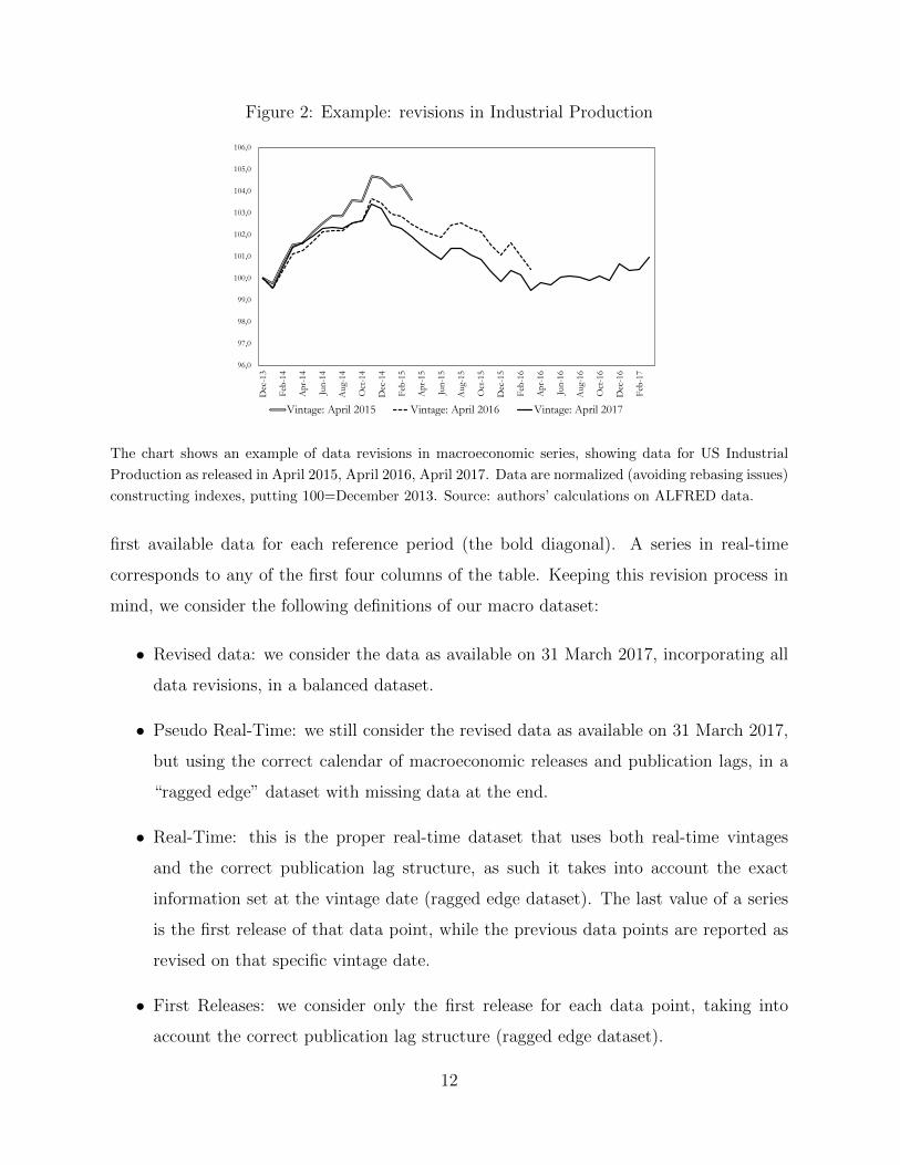
Figure 2: Example: revisions in Industrial Production

96,0

97,0

98,0

99,0

100,0

101,0

102,0

103,0

104,0

105,0

106,0

Dec

-13

Feb

-14

Ap

r-14

Jun

-14

Aug-

14

Oct

-14

Dec

-14

Feb

-15

Ap

r-15

Jun

-15

Aug-

15

Oct

-15

Dec

-15

Feb

-16

Ap

r-16

Jun

-16

Aug-

16

Oct

-16

Dec

-16

Feb

-17

Vintage: April 2015 Vintage: April 2016 Vintage: April 2017

The chart shows an example of data revisions in macroeconomic series, showing data for US Industrial

Production as released in April 2015, April 2016, April 2017. Data are normalized (avoiding rebasing issues)

constructing indexes, putting 100=December 2013. Source: authors’ calculations on ALFRED data.

first available data for each reference period (the bold diagonal). A series in real-time

corresponds to any of the first four columns of the table. Keeping this revision process in

mind, we consider the following definitions of our macro dataset:

• Revised data: we consider the data as available on 31 March 2017, incorporating all

data revisions, in a balanced dataset.

• Pseudo Real-Time: we still consider the revised data as available on 31 March 2017,

but using the correct calendar of macroeconomic releases and publication lags, in a

“ragged edge” dataset with missing data at the end.

• Real-Time: this is the proper real-time dataset that uses both real-time vintages

and the correct publication lag structure, as such it takes into account the exact

information set at the vintage date (ragged edge dataset). The last value of a series

is the first release of that data point, while the previous data points are reported as

revised on that specific vintage date.

• First Releases: we consider only the first release for each data point, taking into

account the correct publication lag structure (ragged edge dataset).

12

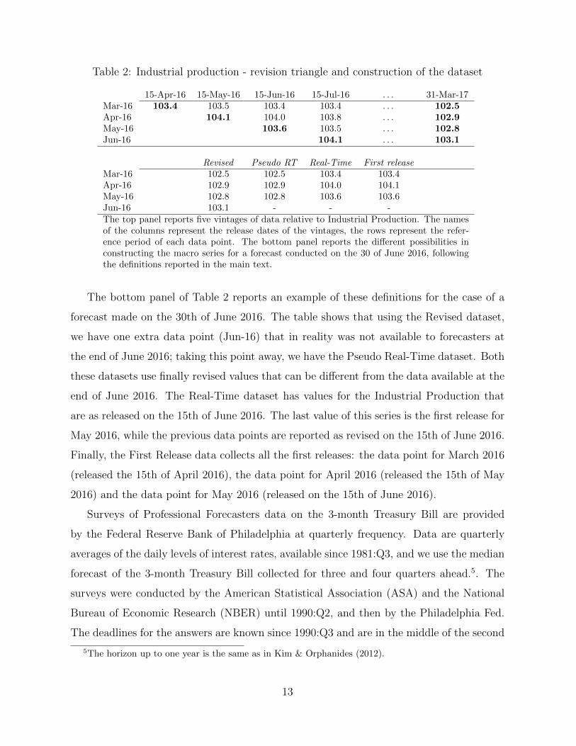
Table 2: Industrial production - revision triangle and construction of the dataset

15-Apr-16 15-May-16 15-Jun-16 15-Jul-16 . . . 31-Mar-17Mar-16 103.4 103.5 103.4 103.4 . . . 102.5Apr-16 104.1 104.0 103.8 . . . 102.9May-16 103.6 103.5 . . . 102.8Jun-16 104.1 . . . 103.1

Revised Pseudo RT Real-Time First releaseMar-16 102.5 102.5 103.4 103.4Apr-16 102.9 102.9 104.0 104.1May-16 102.8 102.8 103.6 103.6Jun-16 103.1 - - -The top panel reports five vintages of data relative to Industrial Production. The namesof the columns represent the release dates of the vintages, the rows represent the refer-ence period of each data point. The bottom panel reports the different possibilities inconstructing the macro series for a forecast conducted on the 30 of June 2016, followingthe definitions reported in the main text.

The bottom panel of Table 2 reports an example of these definitions for the case of a

forecast made on the 30th of June 2016. The table shows that using the Revised dataset,

we have one extra data point (Jun-16) that in reality was not available to forecasters at

the end of June 2016; taking this point away, we have the Pseudo Real-Time dataset. Both

these datasets use finally revised values that can be different from the data available at the

end of June 2016. The Real-Time dataset has values for the Industrial Production that

are as released on the 15th of June 2016. The last value of this series is the first release for

May 2016, while the previous data points are reported as revised on the 15th of June 2016.

Finally, the First Release data collects all the first releases: the data point for March 2016

(released the 15th of April 2016), the data point for April 2016 (released the 15th of May

2016) and the data point for May 2016 (released on the 15th of June 2016).

Surveys of Professional Forecasters data on the 3-month Treasury Bill are provided

by the Federal Reserve Bank of Philadelphia at quarterly frequency. Data are quarterly

averages of the daily levels of interest rates, available since 1981:Q3, and we use the median

forecast of the 3-month Treasury Bill collected for three and four quarters ahead.5. The

surveys were conducted by the American Statistical Association (ASA) and the National

Bureau of Economic Research (NBER) until 1990:Q2, and then by the Philadelphia Fed.

The deadlines for the answers are known since 1990:Q3 and are in the middle of the second

5The horizon up to one year is the same as in Kim & Orphanides (2012).

13

month of the quarter. Since the deadlines for the respondents define their information set,

we fix the release dates in correspondence to those deadlines on the 15th of the second

month of the quarter.

4 Estimation and preliminary results

The mixed-frequency real-time macro-yields model in equations (7)-(9) can be cast in

a state-space form by augmenting the state variables to include the intercept and the

idiosyncratic components, for details see Appendix A.1. Following Doz et al. (2012), we

estimate the model by quasi-maximum likelihood using an Expectation-Maximization (EM)

algorithm initialized by Principal Components. The complication of having a ragged edge

data set, which involves missing data also at the end of the sample, can be solved by

adapting the EM algorithm to the presence of missing data, as in Banbura & Modugno

(2014). Also, the factor loading restrictions that identify the yield curve factors can be

imposed by performing a constrained maximization in the EM algorithm, for more details

see Appendix A.2.

For comparison, we also estimate an only-yields model, which uses only the information

contained in yields. This is a restricted version of the macro-yields model in Equations

(7)-(9) with Γxy = 0, Ayx = 0 and Qyx = 0, and can hence be estimated using the same

procedure.

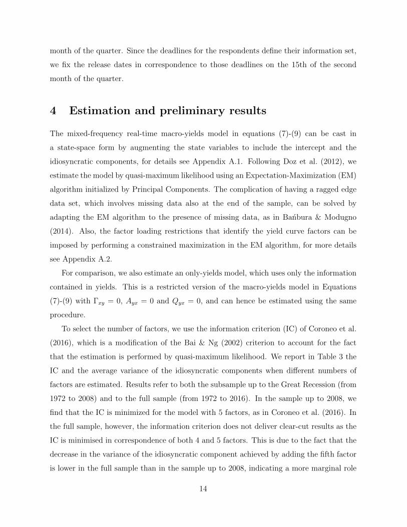
To select the number of factors, we use the information criterion (IC) of Coroneo et al.

(2016), which is a modification of the Bai & Ng (2002) criterion to account for the fact

that the estimation is performed by quasi-maximum likelihood. We report in Table 3 the

IC and the average variance of the idiosyncratic components when different numbers of

factors are estimated. Results refer to both the subsample up to the Great Recession (from

1972 to 2008) and to the full sample (from 1972 to 2016). In the sample up to 2008, we

find that the IC is minimized for the model with 5 factors, as in Coroneo et al. (2016). In

the full sample, however, the information criterion does not deliver clear-cut results as the

IC is minimised in correspondence of both 4 and 5 factors. This is due to the fact that the

decrease in the variance of the idiosyncratic component achieved by adding the fifth factor

is lower in the full sample than in the sample up to 2008, indicating a more marginal role

14

Table 3: Model selection

1972-2008 1972-2016N. of factors IC V IC V

3 -0.05 0.43 -0.06 0.434 -0.16 0.30 -0.15 0.305 -0.22 0.21 -0.15 0.236 -0.19 0.17 -0.10 0.197 -0.07 0.15 0.01 0.168 0.06 0.13 0.09 0.13

Note: the table reports the IC criterion relative tomodels with different numbers of factors, followingthe modified version of the Bai & Ng (2002) crite-rion described in Coroneo et al. (2016). Columns ICreport the information criteria, columns V report theaverage variance of the idiosyncratic components.

of the fifth factor in the last part of the sample. Therefore, after 2008, we select the more

parsimonious model, with four factors.

5 Out-of-sample forecast

We design a forecasting exercise in a truly real-time out-of-sample fashion. We perform a

recursive estimation using data starting in January 1972 and use the out-of-sample eval-

uation period from January 1995 to December 2016. We reconstruct the information set

available to forecasters at each point in time in which the forecast is computed, that is at

the end of each month of the out-of-sample period, using the information available at that

time. This entails using the real-time vintages for all the variables in the dataset, and also

reconstructing the exact calendar of the releases. Since the macroeconomic data releases are

not synchronous, we have to deal with the ragged edge of the dataset: as stated above, the

estimation performed within an Expectation-Maximization algorithm conveniently helps

us in this respect.

Being aware of the presence of the zero lower bound for interest rates, a serious issue

since 2008, we impose non-negativity of the predicted interest rates as follows

Et(y(τ)t+h) ≡ yt+h|t = max(Γy∗|t F

∗t+h|t, 0)

15

where Γy∗|t contains the factor loadings for yields and is estimated using information up to

time t and F ∗t+h|t ≡ Et(F∗t+h) is the out-of-sample iterative forecast of the factors.6 We take

as benchmark the forecast at horizon h for the maturity τ produced by a random walk at

time t

Et(y(τ)t+h) ≡ y

(τ)t+h|t = y

(τ)t .

6 Results

Our empirical results are organised into two parts. First, we assess the predictive content

of real-time macroeconomic information for interest rates by comparing the out-of-sample

performance of a macro-yield model in real-time with one that uses revised macro data.

We then add the interest rate surveys into the model, and analyse their role over and above

real-time macroeconomic information.

6.1 Real-time macro data: is it useful?

In order to assess the role of the real-time macroeconomic data-flow for interest rate pre-

dictions, in this section, we report the out-of-sample evaluation of the macro-yields model

using real-time data.

In Table 4, we report the MSFE (relative to the random walk) of the only-yields model,

the macro-yields model using revised macro data and the macro-yields model using real-

time macro data. We test for the significance of their outperformance with respect to the

random walk using the Diebold & Mariano (2002) test statistic with fixed-b asymptotics

to avoid size distortions due to small sample size and autocorrelation in the loss differen-

tials, see Coroneo & Iacone (2015). Results indicate that macroeconomic data has a strong

predictive ability for interest rates especially at long forecasting horizons and short-mid

maturities, while the only-yields model never outperforms the random walk. The forecast-

ing ability is stronger using revised data, but robust to the use of real-time macro data: the

real-time macro-yields model forecasts significantly better than the random walk at short

maturities for mid-long forecasting horizons.

6See Appendix A.2 for the definitions of Γ∗ and F ∗t .

16

Table 4: Relative MSFE, Evaluation: 1995-2016

Only-yields model3m 6m 1y 2y 3y 4y 5y 7y 10y

1 1.02 1.04 1.02 1.05 1.05 1.04 1.04 1.04 1.023 1.06 1.10 1.07 1.12 1.12 1.11 1.10 1.10 1.056 1.06 1.13 1.13 1.21 1.21 1.20 1.19 1.18 1.1212 1.05 1.10 1.12 1.28 1.35 1.38 1.38 1.37 1.2324 1.13 1.15 1.13 1.33 1.51 1.64 1.75 1.91 1.80

Macro-yields model3m 6m 1y 2y 3y 4y 5y 7y 10y

1 0.84 0.89 0.98 1.03 1.04 1.04 1.03 1.03 1.023 0.72* 0.78* 0.93 1.03 1.05 1.05 1.04 1.03 1.006 0.64** 0.70* 0.81* 0.95 1.00 1.01 1.02 1.01 0.9712 0.60** 0.64** 0.70** 0.82* 0.94 1.00 1.04 1.05 0.9824 0.62** 0.64** 0.65** 0.76* 0.91 1.03 1.15 1.29 1.27

Real-time macro-yields model3m 6m 1y 2y 3y 4y 5y 7y 10y

1 0.90 0.93 0.98 1.06 1.06 1.05 1.04 1.03 1.023 0.79 0.85 1.00 1.07 1.08 1.07 1.06 1.04 1.006 0.71** 0.78* 0.90 0.95 1.05 1.05 1.05 1.03 0.9712 0.69** 0.73* 0.81* 0.93 1.04 1.08 1.10 1.10 1.0024 0.71* 0.73* 0.74* 0.87 1.03 1.15 1.26 1.38 1.32Note: The table reports the relative Mean Squared Forecast Error rela-tive to the random walk of the only-yields model (top panel), the macro-yields model (middle panel) and the Real-time macro-yields model (bot-tom panel), for the evaluation period 1995-2016. A number smaller thanone indicates that the model performs better than the random walk.(*) and (**) indicate one-side significance at the 10% and 5%, respec-tively, using the Diebold & Mariano (2002) test statistic with fixed-basymptotics, as in Coroneo & Iacone (2015).

In order to understand the drivers of the difference in the forecasting performance

between revised and real-time macroeconomic information, in Figure 3 we plot the Mean

Squared Forecast Error of the macro-yields model using the four different definitions of

the macroeconomic dataset described in Section 3: the revised, the pseudo real-time, the

real-time and the first releases datasets. Results indicate that the macro-yields model

consistently outperforms the random walk at short maturities for all horizons. The real-

time macro-yields model is slightly worse than the macro-yields using revised data and

pseudo real-time data, but it still outperforms the random walk at short maturities for

all horizons: this indicates that macroeconomic information is useful in predicting interest

rates, even when using real-time data. Taking into account only the publication lags plays a

17

Figure 3: Real-time macroeconomic information

Mean Squared Forecast Error for the macro-yields model with revised data (MY Rev), the macro-yields

model with pseudo real-time data (MY PRT), the macro-yields model with truly real-time data (MY RT),

the macro-yields model with first releases (MY FR), and the random walk. Evaluation period 1995-2016.

lesser role, since the model in pseudo real-time has a forecasting performance very similar

to the one with revised data. The model that uses the first releases, instead, performs

worse than the others: this is consistent with the intuition that revisions improve the

quality of macroeconomic data and therefore the signal they convey about the future path

of interest rates. Therefore, we can conclude that the main drivers of the difference in

forecasting performance between the model that uses revised macro data and the one that

uses real-time macro data are the data revisions.

Our results are different from the general message of Ghysels et al. (2017)7. In addition

to the finding that a real-time dataset is significantly less powerful in such a forecasting

exercise (our results are milder in this respect), they also find that it also performs worse

than a dataset with first releases. However, their estimation method cannot take into

account missing variables, so the information set cannot exactly represent the information

set faced by a forecaster in real-time. For this reason, their definition of a “real-time”

dataset corresponds to our definition of “first releases”, lagged by one period (for macro

7Note that their analysis refers to excess returns, and is based on a different sample.

18

Figure 4: Forecasts: macro-yield model in real-time vs. interest rate surveys

The charts report the 12-month ahead forecast for the 3-month interest rate obtained from the macro-yield

model in real-time (MY-RT, dashed line), the four-quarters ahead survey for the quarterly average of the

3-month Treasury Bill (Survey Data), and the realised value (Actual, solid line).

variables with a “standard” publication lag, like Industrial Production). Our method,

instead, which relies on filtering techniques widely used in the nowcasting literature (see

Banbura et al. (2013) for details), can efficiently incorporate missing variables and properly

treat a ragged edge dataset, maintaining the contemporaneous relationships between macro

variables and interest rates.

6.2 Interest rate surveys: do they help?

We now add the Surveys of Professional Forecasters data on the 3-month Treasury Bill to

our real-time dataset, in order to evaluate if they contain additional information to predict

the yield curve. We recall that we use the median forecast of the 3-month Treasury Bill

collected for three and four quarters ahead. In fact, we assume that at this horizon soft

information about monetary policy can play a strong role, especially during periods in

which the FOMC uses forward guidance.

In Figure 4, we report the 12-month ahead forecast for the 3-month interest rate ob-

tained from the macro-yield model in real-time, along with the four-quarters ahead survey

for the quarterly average of the 3-month Treasury Bill, and the realised value. The fig-

ure shows how the macro-yield model is able to provide predictions that are closer to the

19

realised value than the survey forecasts from 2007Q3 up to 2012Q2. After this date, the

surveys consistently predict very low values for the 3-month rate, and these predictions

are correct. Only at the very end of the sample, the macro-yield model in real-time pro-

vides more accurate predictions than the surveys again. This is due to the fact that on

August 9, 2011 the FOMC announced that it would likely keep the federal funds rate at

exceptionally low levels “at least through mid-2013”. In the figure, we can see the effect of

the announcement on the decline of the survey forecast for 2012Q3, which was formed one

year ahead, i.e. just after the forward guidance announcement. The figure also shows that

forward guidance announcements have been effective at stabilizing expectations up to mid-

2014 when the one-year ahead predictions for mid-2015 indicated a rise in interest rates.

On the other hand, the macro-yield model in real-time could not incorporate this type of

announcement, and for all this period predicted low interest rates but higher than expected

from the survey. Notice also that the time varying relative importance of model-based and

survey-based forecasts signals the advantage of efficiently combining the different sources

of information.

In Figure 5 we give an intuitive example of the mechanism for which the use of surveys

helps to improve the forecasts of the model. In the top panel, we report the 13-month ahead

forecasts from the only-yields and the real-time macro-yields model (both with and without

the interest rate surveys) made in January 2012, along with the actual realization of the

yield curve in February 2013. In the bottom panel, we report the forecasts for February

2013 made one month later, i.e. in February 2012. In between, there have been some

macroeconomic releases and revisions, which induced the revisions of the forecasts made

using the macro-yields model, but more importantly, there has been an FOMC release with

a “forward guidance type” announcement on the 25th of January 2012.8 In February, the

macroeconomic news releases (and the revisions) brought up the forecasts produced by

the macro-yields model (solid blue line), but the forecasts obtained using the information

in the surveys are lower and closer to the realised values. Notice how, despite including

8The statement reads as follows ”(...) the Committee decided today to keep the target range forthe federal funds rate at 0 to 1/4 percent and currently anticipates that economic conditions–includinglow rates of resource utilization and a subdued outlook for inflation over the medium run–are likely towarrant exceptionally low levels for the federal funds rate at least through late 2014.” Source: https:

//www.federalreserve.gov/newsevents/pressreleases/monetary20120125a.htm.

20

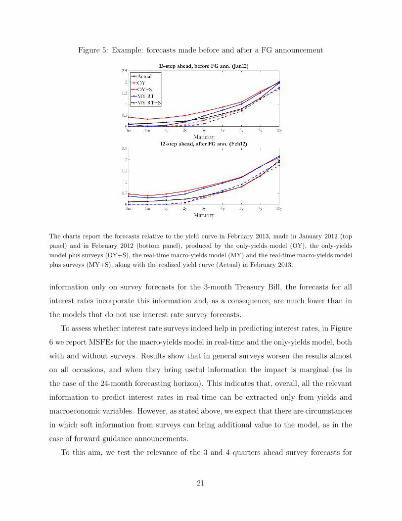
Figure 5: Example: forecasts made before and after a FG announcement

The charts report the forecasts relative to the yield curve in February 2013, made in January 2012 (top

panel) and in February 2012 (bottom panel), produced by the only-yields model (OY), the only-yields

model plus surveys (OY+S), the real-time macro-yields model (MY) and the real-time macro-yields model

plus surveys (MY+S), along with the realized yield curve (Actual) in February 2013.

information only on survey forecasts for the 3-month Treasury Bill, the forecasts for all

interest rates incorporate this information and, as a consequence, are much lower than in

the models that do not use interest rate survey forecasts.

To assess whether interest rate surveys indeed help in predicting interest rates, in Figure

6 we report MSFEs for the macro-yields model in real-time and the only-yields model, both

with and without surveys. Results show that in general surveys worsen the results almost

on all occasions, and when they bring useful information the impact is marginal (as in

the case of the 24-month forecasting horizon). This indicates that, overall, all the relevant

information to predict interest rates in real-time can be extracted only from yields and

macroeconomic variables. However, as stated above, we expect that there are circumstances

in which soft information from surveys can bring additional value to the model, as in the

case of forward guidance announcements.

To this aim, we test the relevance of the 3 and 4 quarters ahead survey forecasts for

21

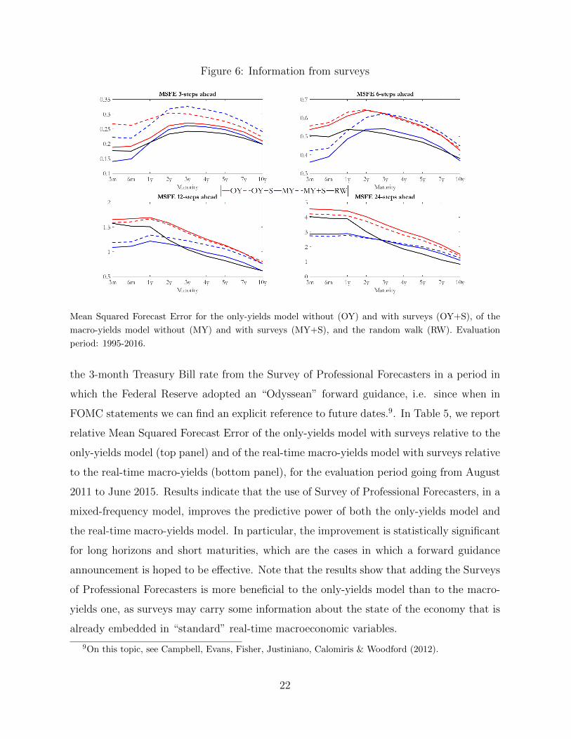
Figure 6: Information from surveys

Mean Squared Forecast Error for the only-yields model without (OY) and with surveys (OY+S), of the

macro-yields model without (MY) and with surveys (MY+S), and the random walk (RW). Evaluation

period: 1995-2016.

the 3-month Treasury Bill rate from the Survey of Professional Forecasters in a period in

which the Federal Reserve adopted an “Odyssean” forward guidance, i.e. since when in

FOMC statements we can find an explicit reference to future dates.9. In Table 5, we report

relative Mean Squared Forecast Error of the only-yields model with surveys relative to the

only-yields model (top panel) and of the real-time macro-yields model with surveys relative

to the real-time macro-yields (bottom panel), for the evaluation period going from August

2011 to June 2015. Results indicate that the use of Survey of Professional Forecasters, in a

mixed-frequency model, improves the predictive power of both the only-yields model and

the real-time macro-yields model. In particular, the improvement is statistically significant

for long horizons and short maturities, which are the cases in which a forward guidance

announcement is hoped to be effective. Note that the results show that adding the Surveys

of Professional Forecasters is more beneficial to the only-yields model than to the macro-

yields one, as surveys may carry some information about the state of the economy that is

already embedded in “standard” real-time macroeconomic variables.

9On this topic, see Campbell, Evans, Fisher, Justiniano, Calomiris & Woodford (2012).

22

Table 5: The usefulness of SPF (RMSFE, August 2011 to June 2015)

(OnlyYields with SPF) vs OnlyYields3m 6m 1y 2y 3y 4y 5y 7y 10y

1 1.13 1.41 1.89 1.32 1.1 1.06 1.04 1.03 1.053 0.48* 0.72 0.87 1.04 0.98 0.99 1.00 0.98 1.056 0.11** 0.3** 0.52 0.73 0.92 1.04 1.08 1.03 1.1512 0.05** 0.17** 0.45* 0.62 0.91 1.04 1.08 1.07 1.1924 0.25** 0.19** 0.23** 0.51** 0.81 1.00 1.07 1.05 1.18

(RT MacroYields with SPF) vs RT MacroYields3m 6m 1y 2y 3y 4y 5y 7y 10y

1 1.23 2.41 2.13 1.23 1.06 1.02 1.01 1.00 1.003 0.74** 1.14 1.25 1.21 1.03 1.04 1.02 1.00 1.036 0.49** 0.61* 0.68 0.99 1.00 1.10 1.09 1.04 1.0812 0.34** 0.33** 0.44* 0.65 0.75 0.83 0.86 0.88 0.9424 0.87 0.87 0.87 0.91 0.93 0.95 0.96 0.94 0.98Note: The table reports the relative Mean Squared Forecast Error of the only-yieldsmodel with SPF relative to the only-yields model (top panel) and of the macro-yields model with SPF relative to the macro-yields (bottom panel), for the evaluationperiod Aug2011-Jun2015. A number smaller than one indicates that the model withSPF performs better. (*) and (**) indicate one-side significance at 10% and 5%,respectively, Diebold and Mariano (1995) test statistic with fixed-b asymptotics, asin Coroneo and Iacone (2018).

7 Conclusions

In this paper, we assess the predictive ability of real-time macroeconomic information and

interest rates surveys for the yield curve of interest rates. We propose a mixed-frequency

dynamic factor model with restrictions on the factor loadings which includes Treasury

yields, a set of real-time macroeconomic variables and interest rate survey expectations.

Through the lens of a real-time out-of-sample exercise, we document the following findings.

First, we show the importance of macroeconomic information in predicting interest rates

in a fully real-time out-of-sample exercise in which, in order to reconstruct the information

set available to market participants at each point in time, we use the real-time vintages

and the exact calendar of data releases.

Second, we document that survey expectations can play an important role in improving

interest rate forecasts at long horizons for short maturities. An interpretation of this find-

ing is that surveys incorporate soft information which might be neglected in “standard”

data: for example, they can consider forward-looking information coming from policy an-

nouncements (e.g. forward guidance). In fact, we prove that properly adding surveys to our

model in a forward guidance period significantly enhances its predictive power, especially

23

for short maturities.

In future research, we plan to extend our empirical specification to explicitly incorporate

long-run trends, to account for the recent decline in interest rates. The macro-yields model

presented in this paper cannot identify trends as it is estimated on real-time macroeconomic

variables transformed to achieve stationarity; however, our model can be easily extended

to deal with trends along the lines of Del Negro, Giannone, Giannoni & Tambalotti (2017).

24

References

Altavilla, C., Giacomini, R. & Ragusa, G. (2017), ‘Anchoring the yield curve using survey

expectations’, Journal of Applied Econometrics 32(6), 1055–1068.

Ang, A. & Piazzesi, M. (2003), ‘A No-Arbitrage Vector Autoregression of Term Structure

Dynamics with Macroeconomic and Latent Variables’, Journal of Monetary Economics

50(4), 745–787.

Bai, J. & Ng, S. (2002), ‘Determining the Number of Factors in Approximate Factor Mod-

els’, Econometrica 70(1), 191–221.

Banbura, M., Giannone, D., Modugno, M. & Reichlin, L. (2013), ‘Now-casting and the

real-time data flow’, Handbook of economic forecasting 2(Part A), 195–237.

Banbura, M. & Modugno, M. (2014), ‘Maximum likelihood estimation of factor models

on datasets with arbitrary pattern of missing data’, Journal of Applied Econometrics

29(1), 133–160.

Boivin, J. & Ng, S. (2006), ‘Are more data always better for factor analysis?’, Journal of

Econometrics 132(1), 169–194.

Campbell, J. R., Evans, C. L., Fisher, J. D., Justiniano, A., Calomiris, C. W. & Woodford,

M. (2012), ‘Macroeconomic effects of Federal Reserve forward guidance’, Brookings

Papers on Economic Activity pp. 1–80.

Coroneo, L., Giannone, D. & Modugno, M. (2016), ‘Unspanned macroeconomic factors in

the yield curve’, Journal of Business & Economic Statistics 34(3), 472–485.

Coroneo, L. & Iacone, F. (2015), ‘Comparing predictive accuracy in small samples using

fixed-smoothing asymptotics’, York Discussion Paper 15.

Coroneo, L., Nyholm, K. & Vidova-Koleva, R. (2011), ‘How arbitrage-free is the Nelson–

Siegel model?’, Journal of Empirical Finance 18(3), 393–407.

Croushore, D. & Stark, T. (2003), ‘A real-time data set for macroeconomists: Does the

data vintage matter?’, Review of Economics and Statistics 85(3), 605–617.

25

Del Negro, M., Giannone, D., Giannoni, M. P. & Tambalotti, A. (2017), ‘Safety, liq-

uidity, and the natural rate of interest’, Brookings Papers on Economic Activity

2017(1), 235–316.

Diebold, F. X. & Li, C. (2006), ‘Forecasting the term structure of government bond yields’,

Journal of Econometrics 130, 337–364.

Diebold, F. X. & Mariano, R. S. (2002), ‘Comparing predictive accuracy’, Journal of

Business & Economic Statistics 20(1), 134–144.

Doz, C., Giannone, D. & Reichlin, L. (2012), ‘A quasi-maximum likelihood approach for

large, approximate dynamic factor models’, The Review of Economics and Statistics

94(4), 1014–1024.

Favero, C. A., Niu, L. & Sala, L. (2012), ‘Term structure forecasting: No-arbitrage restric-

tions versus large information set’, Journal of Forecasting 31(2), 124–156.

Ghysels, E., Horan, C. & Moench, E. (2017), ‘Forecasting through the rearview mir-

ror: Data revisions and bond return predictability’, The Review of Financial Studies

31(2), 678–714.

Giannone, D., Reichlin, L. & Small, D. (2008), ‘Nowcasting: The real-time informational

content of macroeconomic data’, Journal of Monetary Economics 55(4), 665–676.

Kim, D. H. & Orphanides, A. (2012), ‘Term structure estimation with survey data on

interest rate forecasts’, Journal of Financial and Quantitative Analysis 47(1), 241–

272.

Koenig, E. F., Dolmas, S. & Piger, J. (2003), ‘The use and abuse of real-time data in

economic forecasting’, Review of Economics and Statistics 85(3), 618–628.

Ludvigson, S. C. & Ng, S. (2009), ‘Macro factors in bond risk premia’, Review of Financial

Studies 22(12), 5027.

Monch, E. (2008), ‘Forecasting the yield curve in a data-rich environment: A no-arbitrage

factor-augmented var approach’, Journal of Econometrics 146(1), 26–43.

26

Nelson, C. R. & Siegel, A. F. (1987), ‘Parsimonious modeling of yield curves’, Journal of

Business 60, 473–89.

Orphanides, A. (2001), ‘Monetary policy rules based on real-time data’, American

Economic Review 91(4), 964–985.

Orphanides, A. & Van Norden, S. (2002), ‘The unreliability of output-gap estimates in real

time’, Review of Economics and Statistics 84(4), 569–583.

27

A APPENDIX - Estimation procedure

A.1 State-space representation

The mixed-frequency macro-yields model with real-time macro information in equations (7)-

(9) can be cast in a state-space form by augmenting the state variables to include the

intercept and the idiosyncratic components. In particular, the measurement equation can

be written as

yt

xt

Es(yqt )

=

ΓNSyy 0 0 0 In 0 0

Γxy Γyy 0 ax 0 Im 0

0 0 Γq as 0 0 Is

F yt

F xt

F qt

ct

vyt

vxt

vst

+

ηyt

ηxt

ηst

(10)

where (ηyt , ηxt , η

st )′ ∼ N(0, εIn+m+s) with ε a very small fixed coefficient. ΓNSyy is the matrix

whose rows correspond to the smooth patterns proposed by Nelson & Siegel (1987) and

shown in equation (2). Also notice that, since we are using real-time macro data, xt contains

missing values.

If we denote by Ft = [F yt , F

xt ] and vt = [vyt , v

xt ], then we can write the state equation as

Ft

F qt

ct

vt

vst

=

A 0 µ 0 0

wtA ιtIr wtµ 0 0

0 0 1 0 0

0 0 0 B 0

0 0 0 0 Bs

Ft−1

F qt−1

ct−1

vt−1

vst−1

+

ut

ust

νt

ξt

ξst

(11)

with (ut, ust , νt, ξt, ξ

st )′ ∼ N (0, blkdiag(Q,w′tQwt, ε, R,Rs)) and where the coefficients wt

and ιt are known (wt is equal to 1, 1/2, 1/3 and ιt is equal to 0, 1/2, 2/3 respectively the

first, second and third month of the quarter). In this state-space form, ct an additional

state variable restricted to one at every time t.

28

A.2 Estimation

The state-space model in (10)-(11) can be written compactly as

zt = Γ∗F ∗t + v∗t , v∗t ∼ N(0, R∗)

F ∗t = A∗tF∗t−1 + u∗t , u∗t ∼ N(0, Q∗t )

where zt =

yt

xt

Es(yqt )

, F ∗t =

Ft

F qt

ct

vt

vst

, v∗t =

ηyt

ηxt

ηst

and u∗t =

ut

ust

εt

ξt

ξst

.

The restrictions on the factor loadings Γ∗ and on the transition matrix A∗t can be written

as

H1 vec(Γ∗) = q1, H2 vec(A∗t ) = q2t,

where H1 and H2 are selection matrices, and q1 and q2t contain the restrictions.

We assume that F ∗1 ∼ N(π1, V1), and define z = [z1, . . . , zT ] and F ∗ = [F ∗1 , . . . , F∗T ].

Then denoting the parameters by θt = {Γ∗, A∗t , Q∗t , π1, V1}, we can write the joint loglikeli-

hood of zt and Ft, for t = 1, . . . , T , as

L(z, F ∗; θ) = −T∑t=1

(1

2[zt − Γ∗F ∗t ]′ (R∗)−1 [zt − Γ∗F ∗t ]

)+

−T2

log |R∗| −T∑t=2

(1

2[F ∗t − A∗tF ∗t−1]′(Q∗t )

−1[F ∗t − A∗tF ∗t−1]

)+

−T − 1

2log |Q∗t |+

1

2[F ∗1 − π1]′V −1

1 [F ∗1 − π1] +

−1

2log |V1| −

T (p+ k)

2log 2π + λ′1 (H1 vec(Γ∗)− q1) + λ′2 (H2 vec(A∗t )− q2)

where λ1 contains the lagrangian multipliers associate with the constraints on the factor

loadings Γ∗ and λ2 contains the lagrangian multipliers associated with the constraints on

the transition matrix A∗t .

The computation of the Maximum Likelihood estimates is performed using the EM

29

algorithm. Broadly speaking, the algorithm consists in a sequence of simple steps, each of

which uses the time-varying parameter Kalman smoother to extract the common factors

for a given set of parameters and closed form solutions to estimate the parameters given

the factors. In practice, we use the restricted version of the EM algorithm, the Expectation

Restricted Maximization, since we need to impose the smooth pattern on the factor loadings

of the yields on the Nelson-Siegel factors. The ERM algorithm alternates Kalman filter

extraction of the factors to the restricted maximization of the likelihood. At the j-th

iteration the ERM algorithm performs two steps:

1. In the Expectation-step, we compute the expected log-likelihood conditional on the

data and the estimates from the previous iteration, i.e.

L(θ) = E[L(z, F ∗; θ(j−1))|z]

which depends on three expectations

F ∗t ≡ E[F ∗t ; θ(j−1)|z]

Pt ≡ E[F ∗t (F ∗t )′; θ(j−1)|z]

Pt,t−1 ≡ E[F ∗t (F ∗t−1)′; θ(j−1)|z]

Given that our observables contain missing values, these expectations can be com-

puted, for given parameters of the model, using the time-varying parameters Kalman

smoother. This entails pre-multiplying the measurement equation by a selection ma-

trix St of dimension (n−#missing)× n, as follows

Stzt = StΓ∗F ∗t + Stv

∗t , Stv

∗t ∼ N(0, StR

∗St)

and apply the Kalman filter to a time-varying measurement equation with parameters

StΓ∗ and StR

∗St, and observables Stzt.

2. In the Restricted Maximization-step, we update the parameters maximizing the ex-

30

pected the expected lagrangian with missing values with respect to θ:

θ(j) = arg maxθL(θ)

This can be implemented taking the corresponding partial derivative of the expected

log likelihood, setting to zero, and solving. In particular, the measurement equation

parameters are estimated by using a selection matrix Wt with diagonal element equal

to 1 if non-missing, and 0 otherwise, so that only the available data are used in the

calculations.

Following Coroneo et al. (2016), we initialize the yield curve factors with the Nelson-

Siegel factors using the two-steps ordinary least squares (OLS) procedure introduced by

Diebold & Li (2006). We then project the balanced panel of macroeconomic variables on the

Nelson-Siegel factors and use the principal components of the residuals of this regression to

initialize the unspanned macroeconomic factors. The quarterly factors are then computed

by time aggregating the monthly yield curve and macro factors. All the parameters are

initialized with the OLS estimates obtained using the initial guesses of yield and macro

factors described above. The initial values for the factor loadings of surveys are obtained

by projecting the linearly interpolated quarterly surveys on the quarterly factors observed

at a monthly frequency.

31