Embed Size (px)
Citation preview

ADDRESS OF PUBLISHER& EDITOR’S OFFICE:
GDAŃSK UNIVERSITYOF TECHNOLOGY
Faculty of Ocean Engineering& Ship TechnologyG. Narutowicza 11/1280-233 Gdańsk, POLAND
tel.: +48 58 347 13 66fax: +48 58 341 13 66
EDITORIAL STAFF:
Jacek Rudnicki | Editor in ChiefPrzemysław Wierzchowski | Scientific EditorJan Michalski | Editor for review mattersAleksander Kniat | Editor for international
relationsKazimierz Kempa | Technical EditorPiotr Bzura | Managing Editor
Price:single issue: 25 zł
Prices for abroadsingle ussue:- in Europe EURO 15- overseas USD 20
WEB:www.bg.pg.gda.pl/pmr/pmr.php
ISSN 1233-2585
3 Krzysztof NausElectronic navigational chart as an equivalent to image produced by hypercatadioptric camera system
10 Stanisław GucmaSTUDYING SEA WATERWAY SYSTEM WITH THE AID OF COMPUTER SIMULATION METHODS
16 Zenon ZwierzewiczThe design of ship autopilot by applying observer - based feedback linearization
22 Weijia Ma, Hanbing Sun, Huawei Sun, Jin Zou, Jiayuan ZhuangTest Studies of the Resistance and Seakeeping Performance of a Trimaran Planing Hull
28 Katarzyna ŻelaznyAn approximate method for calculation of mean statistical value of ship service speed on a given shipping line , useful in preliminary design stage
36 Czesław Dymarski, Paweł Dymarski, Jędrzej ŻywickiDesign and strength calculations of the tripod support structure for offshore power plant
47 Zbigniew KorczewskiEXHAUST GAS TEMPERATURE MEASUREMENTS IN DIAGNOSTICS OF TURBOCHARGED MARINE INTERNAL COMBUSTION ENGINESPART I STANDARD MEASUREMENTS
55 Jacek RudnickiAPPLICATION ISSSUES OF THE SEMI-MARKOV RELIABILITY MODEL
65 Andrzej Grządziela, Janusz Musiał, Łukasz Muślewski, Michał PająkA method for identification of non-coaxiality in engine shaft lines of a selected type of naval ships
72 Wojciech JurczakIMPACT AND BALLISTIC RESISTANCE OF A NEW ALUMINIUM ALLOY FOR SHIP CONSTRUCTION ELEMENTS
No. 1 (85) 2015Vol. 22

EditorialPOLISH MARITIME RESEARCH is a scientific journal of worldwide circulation. The journal appears as a quarterly four times a year. The first issue of it was published in September 1994. Its main aim is to present original, innovative scientific ideas and Research & Development achievements in the field of :
Engineering, Computing & Technology, Mechanical Engineering,
which could find applications in the broad domain of maritime economy. Hence there are published papers which concern methods of the designing, manufacturing and operating processes of such technical objects and devices as : ships, port equipment, ocean engineering units, underwater vehicles and equipment as
well as harbour facilities, with accounting for marine environment protection.The Editors of POLISH MARITIME RESEARCH make also efforts to present problems dealing with education of engineers and scientific and teaching personnel. As a rule, the basic papers are supplemented by information on conferences , important scientific events as well as cooperation in carrying out international
scientific research projects.Scientific Board
Chairman : Prof. JERZY GIRTLER - Gdańsk University of Technology, Poland Vice-chairman : Prof. ANTONI JANKOWSKI - Institute of Aeronautics, Poland
Vice-chairman : Prof. MIROSŁAW L. WYSZYŃSKI - University of Birmingham, United Kingdom
Dr POUL ANDERSENTechnical University of Denmark
Denmark
Dr MEHMET ATLARUniversity of Newcastle United
Kingdom
Prof. GÖRAN BARKChalmers University of Technology
Sweden
Prof. SERGEY BARSUKOVArmy Institute of Odessa Ukraine
Prof. MUSTAFA BAYHANSüleyman Demirel University
Turkey
Prof. VINCENZO CRUPIUniversity of Messina, Italy
Prof. MAREK DZIDAGdańsk University of Technology
Poland
Prof. ODD M. FALTINSENNorwegian University of Science
and TechnologyNorway
Prof. PATRICK V. FARRELLUniversity of Wisconsin Madison,
WIUSA
Prof. WOLFGANG FRICKETechnical University Hamburg-
Harburg Germany
Prof. STANISŁAW GUCMAMaritime University of Szczecin
Poland
Prof. ANTONI ISKRAPoznań University of Technology
Poland
Prof. JAN KICIŃSKIInstitute of Fluid-Flow Machinery
of PASciPoland
Prof. ZYGMUNT KITOWSKINaval University Poland
Prof. JAN KULCZYKWrocław University of Technology
Poland
Prof. NICOS LADOMMATOSUniversity College London United
Kingdom
Prof. JÓZEF LISOWSKIGdynia Maritime University Poland
Prof. JERZY MATUSIAKHelsinki University of Technology
Finland
Prof. EUGEN NEGRUSUniversity of Bucharest Romania
Prof. YASUHIKO OHTANagoya Institute of Technology
Japan
Dr YOSHIO SATONational Traffic Safety and Environment Laboratory
Japan
Prof. KLAUS SCHIERUniversity of Applied Sciences
Germany
Prof. FREDERICK STERNUniversity of Iowa, IA, USA
Prof. JÓZEF SZALABydgoszcz University
of Technology and Agriculture Poland
Prof. TADEUSZ SZELANGIEWICZTechnical University of Szczecin
Poland
Prof. WITALIJ SZCZAGINState Technical University of
KaliningradRussia
Prof. BORIS TIKHOMIROVState Marine University of St.
PetersburgRussia
Prof. DRACOS VASSALOSUniversity of Glasgow and
Strathclyde United Kingdom
POLISH MARITIME RESEARCH, No 1/2015 3
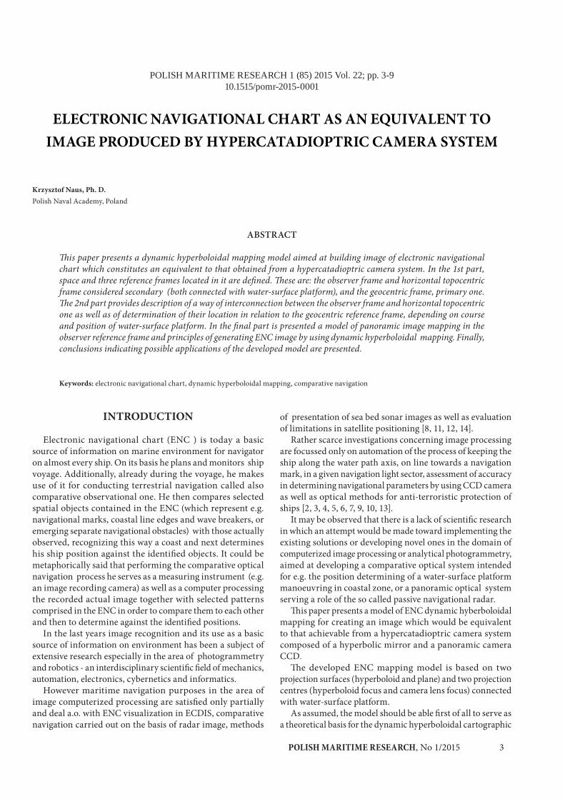
POLISH MARITIME RESEARCH 1 (85) 2015 Vol. 22; pp. 3-910.1515/pomr-2015-0001
ELECTRONIC NAVIGATIONAL CHART AS AN EQUIVALENT TO IMAGE PRODUCED BY HYPERCATADIOPTRIC CAMERA SYSTEM
Krzysztof Naus, Ph. D.Polish Naval Academy, Poland
ABSTRACT
This paper presents a dynamic hyperboloidal mapping model aimed at building image of electronic navigational chart which constitutes an equivalent to that obtained from a hypercatadioptric camera system. In the 1st part, space and three reference frames located in it are defined. These are: the observer frame and horizontal topocentric frame considered secondary (both connected with water-surface platform), and the geocentric frame, primary one.The 2nd part provides description of a way of interconnection between the observer frame and horizontal topocentric one as well as of determination of their location in relation to the geocentric reference frame, depending on course and position of water-surface platform. In the final part is presented a model of panoramic image mapping in the observer reference frame and principles of generating ENC image by using dynamic hyperboloidal mapping. Finally, conclusions indicating possible applications of the developed model are presented.
Keywords: electronic navigational chart, dynamic hyperboloidal mapping, comparative navigation
INTRODUCTION
Electronic navigational chart (ENC ) is today a basic source of information on marine environment for navigator on almost every ship. On its basis he plans and monitors ship voyage. Additionally, already during the voyage, he makes use of it for conducting terrestrial navigation called also comparative observational one. He then compares selected spatial objects contained in the ENC (which represent e.g. navigational marks, coastal line edges and wave breakers, or emerging separate navigational obstacles) with those actually observed, recognizing this way a coast and next determines his ship position against the identified objects. It could be metaphorically said that performing the comparative optical navigation process he serves as a measuring instrument (e.g. an image recording camera) as well as a computer processing the recorded actual image together with selected patterns comprised in the ENC in order to compare them to each other and then to determine against the identified positions.
In the last years image recognition and its use as a basic source of information on environment has been a subject of extensive research especially in the area of photogrammetry and robotics - an interdisciplinary scientific field of mechanics, automation, electronics, cybernetics and informatics.
However maritime navigation purposes in the area of image computerized processing are satisfied only partially and deal a.o. with ENC visualization in ECDIS, comparative navigation carried out on the basis of radar image, methods
of presentation of sea bed sonar images as well as evaluation of limitations in satellite positioning [8, 11, 12, 14].
Rather scarce investigations concerning image processing are focussed only on automation of the process of keeping the ship along the water path axis, on line towards a navigation mark, in a given navigation light sector, assessment of accuracy in determining navigational parameters by using CCD camera as well as optical methods for anti-terroristic protection of ships [2, 3, 4, 5, 6, 7, 9, 10, 13].
It may be observed that there is a lack of scientific research in which an attempt would be made toward implementing the existing solutions or developing novel ones in the domain of computerized image processing or analytical photogrammetry, aimed at developing a comparative optical system intended for e.g. the position determining of a water-surface platform manoeuvring in coastal zone, or a panoramic optical system serving a role of the so called passive navigational radar.
This paper presents a model of ENC dynamic hyberboloidal mapping for creating an image which would be equivalent to that achievable from a hypercatadioptric camera system composed of a hyperbolic mirror and a panoramic camera CCD.
The developed ENC mapping model is based on two projection surfaces (hyperboloid and plane) and two projection centres (hyperboloid focus and camera lens focus) connected with water-surface platform.
As assumed, the model should be able first of all to serve as a theoretical basis for the dynamic hyperboloidal cartographic
POLISH MARITIME RESEARCH, No 1/20154
mapping of ENC, which is dedicated to comparative optical systems to be used in the future on water surface platforms. Secondly, it should provide a theoretical basis for projection of an image available from a panoramic optical system for ship traffic monitoring (which determines position and motion parameters of ships).
DETERMINATION OF SPACE AND REFERENCE FRAMES
Let 3 be 3- dimensional Euclidian space over a body of real numbers R , 3E - associated Euclidian space, O - a point of 3E , a 321 eee ,, - an orthogonal normal base of 3E . The below written system will be called the orthogonal Cartesian reference frame ( a global datum point) of 3Å space:
321 eeeO ,,, . (1)
The point O will determine its origin ( or base point ) and
321 ,, eee - base of the system . Let be the fixed reference frame of the space 3 . The
set of numbers ),,( zyx determines orthogonal Cartesian
coordinates of the point P in relation to the reference frame , and:
321 eeeOPP zyx , (2)
location vector of P against .Let 321 eeeO ,,, and 321 eeeO ,,,
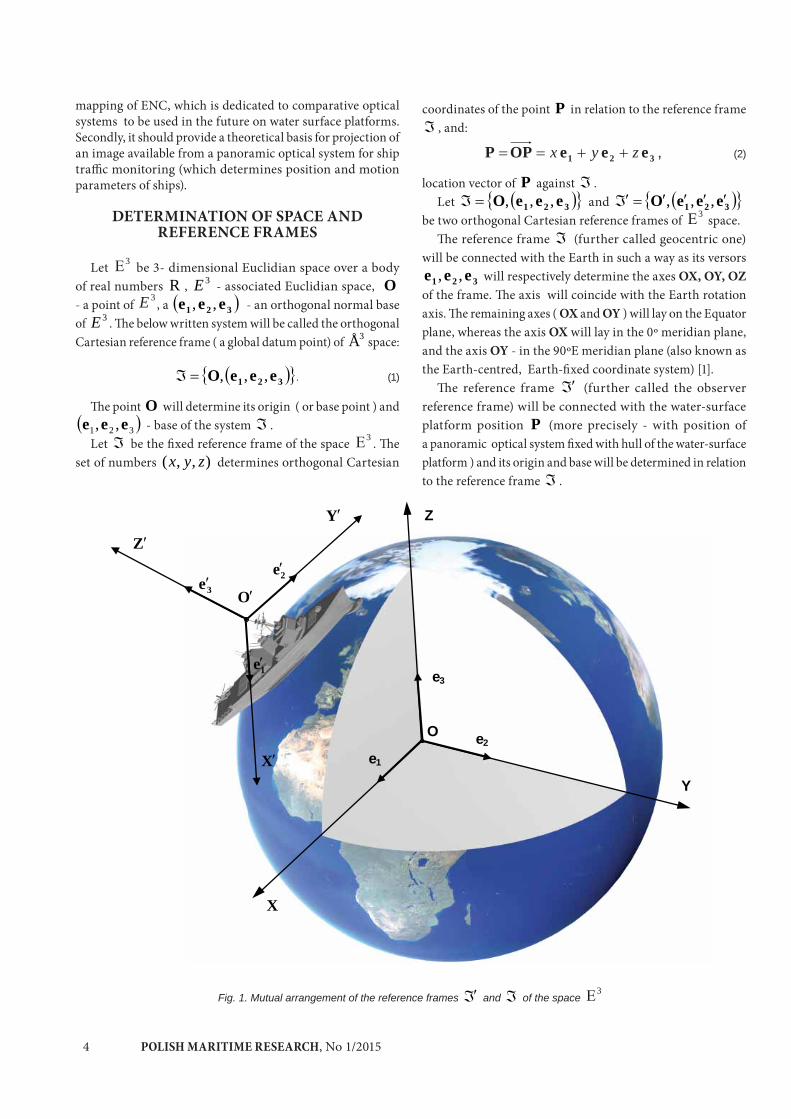
be two orthogonal Cartesian reference frames of 3 space.The reference frame (further called geocentric one)
will be connected with the Earth in such a way as its versors
321 eee ,, will respectively determine the axes OX, OY, OZ of the frame. The axis will coincide with the Earth rotation axis. The remaining axes ( OX and OY ) will lay on the Equator plane, whereas the axis OX will lay in the 0º meridian plane, and the axis OY - in the 90ºE meridian plane (also known as the Earth-centred, Earth-fixed coordinate system) [1].
The reference frame (further called the observer reference frame) will be connected with the water-surface platform position P (more precisely - with position of a panoramic optical system fixed with hull of the water-surface platform ) and its origin and base will be determined in relation to the reference frame .
Z '
Y
X
Z
e2
e1
e3
O
2e
1e
3e
Y
X
Z
O
Fig. 1. Mutual arrangement of the reference frames and of the space 3
POLISH MARITIME RESEARCH, No 1/2015 5
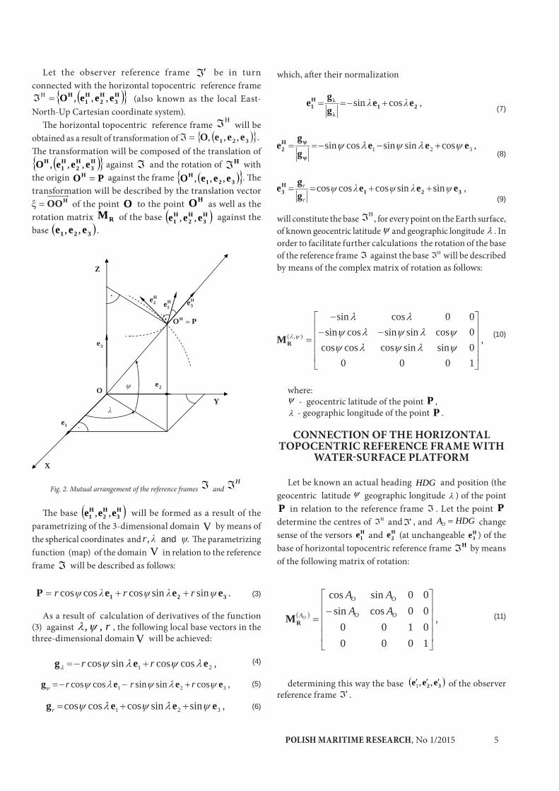
Let the observer reference frame be in turn connected with the horizontal topocentric reference frame
H3
H2
H1
H eeeO ,,,H (also known as the local East-North-Up Cartesian coordinate system).
The horizontal topocentric reference frame H will be obtained as a result of transformation of 321 eeeO ,,, . The transformation will be composed of the translation of
H3
H2
H1
H eeeO ,,, against and the rotation of H with the origin POH against the frame 321
H eeeO ,,, . The transformation will be described by the translation vector
HOO of the point O to the point HO as well as the rotation matrix RM of the base H
3H2
H1 eee ,, against the
base 321 eee ,, .
Fig. 2. Mutual arrangement of the reference frames and H
The base H3
H2
H1 eee ,, will be formed as a result of the
parametrizing of the 3-dimensional domain V by means of the spherical coordinates and r, and . The parametrizing function (map) of the domain V in relation to the reference frame will be described as follows:
(3)
As a result of calculation of derivatives of the function (3) against r,, , the following local base vectors in the three-dimensional domain V will be achieved:
21 coscossincos eeg rr , (4)
(5)
(6)
which, after their normalization
(7)
(8)
(9)
will constitute the base H , for every point on the Earth surface, of known geocentric latitude and geographic longitude . In order to facilitate further calculations the rotation of the base of the reference frame against the base H will be described by means of the complex matrix of rotation as follows:
(10)
where: - geocentric latitude of the point P , - geographic longitude of the point P .
CONNECTION OF THE HORIZONTAL TOPOCENTRIC REFERENCE FRAME WITH
WATER-SURFACE PLATFORM
Let be known an actual heading HDG and position (the geocentric latitude geographic longitude ) of the point P in relation to the reference frame . Let the point P determine the centres of H and , and HDGAO change sense of the versors H
1e and H2e (at unchangeable H
3e ) of the base of horizontal topocentric reference frame H by means of the following matrix of rotation:
(11)
determining this way the base 32 eee ,,1 of the observer reference frame .
X
H3e H
1e
POH
H2e
2e
1e
3e
Z
Y O
321 eeeP rrr sinsincoscoscos .
321 cossinsincoscos eeeg rrr ,
321 sinsincoscoscos eeegr ,
21H1 ee
gge cossin ,
321 cossinsincossin eeegg
eH2 ,
321H3 eee
gge
r
r sinsincoscoscos ,
10000sinsincoscoscos0cossinsincossin00cossin
),(RM ,
1000010000cossin00sincos
OO
OO
A AAAA
ORM ,

POLISH MARITIME RESEARCH, No 1/20156
As assumed, all geometrical transformations will be conducted on the basis of homogeneous, orthogonal Cartesian coordinates which enable to join rotations and simultaneously to scale (dilatation) with translation. In the case of the examined transformations, the assumption will make it possible to join together the rotation matrix OA,,
RM and translation matrix TM ( which represents the vector HOO ). As a result of
combining the two transformations the final complex matrix of geometrical transformations, M , which enables to transform the base and origin of 321 eeeO ,,, into the base and origin of 321 eeeO ,,, , will be obtained:
(13)
(12)
where:
- matrix of translation of the pointO into the point POO' H
Z
O , HO
HDG
North Pole
O
South Pole
3e , H3e
1e , H1e
2e , H2e
Fig. 3. Graphical interpretation of transformation of the base of the horizontal topocentric reference frame H
into the base of the observer reference frame
),(,RRR MMM OO AA,
10000sinsincoscoscos0coscossinsincoscossincossincossinsin0cossinsinsinsincoscossincoscossinsin
AAAAAAAAAA
OOOOO
OOOOO
.
OA,,RT MMM
1000
22
11
030303333
0202022
0101011
zzyyxxzyxzzyyxxzyxzzyyxxzyx
,
The transformation of the base of the reference frame , successively into the base of ,H , will be described by means of the following complex matrix of rotation:
1000100010001
0
0
0
zyx
TM
11 zyx ,, 11e ,
AAx OO1 sincoscossinsin ,
AAy OO sinsinsincoscos1 ,
Az O cossin1 ;
222 zyx ,,2e ,
AAx OO2 cossincossinsin ,
AAy OO sinsincoscossin2 ,
Az O coscos2 ;
POLISH MARITIME RESEARCH, No 1/2015 7
MODEL OF THE PANORAMIC IMAGE MAPPING IN THE OBSERVER REFERENCE
FRAME
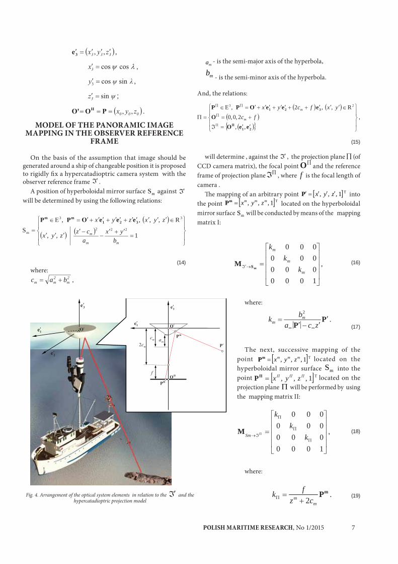
On the basis of the assumption that image should be generated around a ship of changeable position it is proposed to rigidly fix a hypercatadioptric camera system with the observer reference frame .
A position of hyperboloidal mirror surface mS against will be determined by using the following relations:
(14)where:
ma - is the semi-major axis of the hyperbola,
mb - is the semi-minor axis of the hyperbola.
And, the relations:
(15)
will determine , against the , the projection plane (of CCD camera matrix), the focal point O and the reference frame of projection plane , where f is the focal length of camera .
The mapping of an arbitrary point T1,,, zyxP into the point T1,,, mmm zyxmP located on the hyperboloidal mirror surface mS will be conducted by means of the mapping matrix I:
(16)
where:
(17)
The next, successive mapping of the point T1,,, mmm zyxmP located on the hyperboloidal mirror surface mS into the point T1,,, zyxP located on the projection plane will be performed by using the mapping matrix II:
(18)
where:
mPm
m czfk2
. (19)Fig. 4. Arrangement of the optical system elements in relation to the and the hypercatadioptric projection model
1,,
R,,,,S 222
33
m
mm
m
byx
aczzyx
zyxzyx 321mm eeePP
2m
2mm bac ,
21
321
eeO
eeePP
,,
2,0,0
R,,2, 23
fc
yxfcyx
m
m
,
1000000000000
m
m
m
kk
k
mSM ,
PP zca
bkmm
mm
2
.
1000000000000
kk
k
SmM ,
POLISH MARITIME RESEARCH, No 1/20158
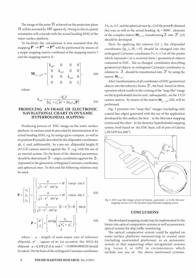
The image of the point achieved on the projection plane will be inverted by 180 against 3e . Owing to this its spatial
orientation will coincide with the actual heading HDG of the water-surface platform.
To facilitate the calculations it was assumed that the mapping m PPP will be performed by means of a single mapping matrix combined of the mapping matrix I and the mapping matrix II:
(20)
where:
(21)
PRODUCING AN IMAGE OF ELECTRONIC NAVIGATIONAL CHART IN DYNAMIC
HYPERBOLOIDAL MAPPING
Producing process of ENC image on the water surface platform in motion must be preceded by determination of its actual heading HDG, e.g. by using a gyro-compass , as well as its position P (usually described by the ellipsoidal coordinates:
, and, additionally, by a pre-set ellipsoidal height H of CCD camera matrix) against the , e.g. with the use of an inertial system. On the basis of the obtained parameters, should be determined - origin coordinates against the , expressed in the geocentric orthogonal Cartesian coordinates and spherical ones. To this end the following relations may be used:
(22)
20
20
0
yxzarctgP ,
(23)
where : a - length of semi-major axis of reference ellipsoid, 2e - square of its 1st eccentric (for WGS-84 ellipsoid 137.0 378 6 a m and 290069438002.02e should be taken). On the basis of the orthogonal Cartesian coordinates
000 zyx ,, and the spherical ones , of the point P, obtained this way, as well as the actual heading HDGAO , elements of the complex matrix M transforming into (13) should be developed.
Next, by applying the relation (22 ), the ellipsoidal coordinates 0,, 111 H should be changed into the orthogonal Cartesian coordinates 111 ,, zyx of all the points which represent ( in a vectorial form ) geometrical objects contained in ENC. The so changed coordinates describing geometrical objects in orthogonal Cartesian coordinates in relation to , should be transformed into by using the matrix M .
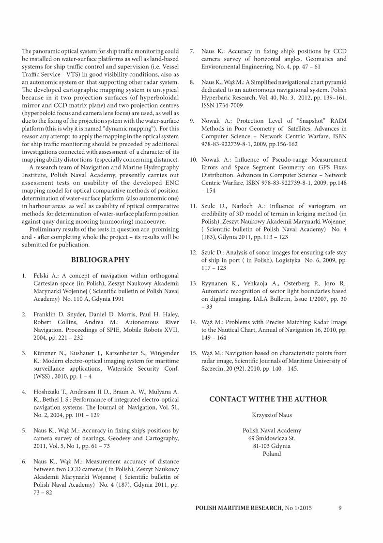
After transformation of all coordinates of ENC geometrical objects into the reference frame , the final , based on them, operation which results in the creating of the “map-like” image on the hyperboloidal mirror and , subsequently , on the CCD camera matrix, by means of the matrix M (20), will be performed.
Fig. 5 presents two “map-like” images (including only coastal line edges) generated with the use of the application developed by this author, the first - in the Mercator mapping system and the other - in the dynamic hyperboloidal mapping system, both based on the ENC basic cell of port of Gdynia („PLGDYNA.000”).
a)
b)
Fig. 5. ENC map-like images of port of Gdynia , generated : a) in the Mercator mapping system, b) in the dynamic hyperboloidal mapping system
CONCLUSIONS
The developed mapping model may be implemented In the future into optical comparative systems as well as panoramic optical systems for ship traffic monitoring.
The optical comparative system could be applied on water-surface platforms manoeuvring in coastal zone (including unattended platforms), as an autonomic system or that supporting other navigational systems (e.g. Loran C or GPS) in circumstances which exclude any use of the above mentioned systems.
1000000000000
m
m
m
kk
k
M ,
Pmmmm
mm cazca
fbk222
2
.
sin
sincos
coscos
0
0
0
He1sine1
a
Hsine1
a
Hsine1
a
zyx
2
22
22
22
P ,
POLISH MARITIME RESEARCH, No 1/2015 9
The panoramic optical system for ship traffic monitoring could be installed on water-surface platforms as well as land-based systems for ship traffic control and supervision (i.e. Vessel Traffic Service - VTS) in good visibility conditions, also as an autonomic system or that supporting other radar system. The developed cartographic mapping system is untypical because in it two projection surfaces (of hyperboloidal mirror and CCD matrix plane) and two projection centres (hyperboloid focus and camera lens focus) are used, as well as due to the fixing of the projection system with the water-surface platform (this is why it is named “dynamic mapping“). For this reason any attempt to apply the mapping in the optical system for ship traffic monitoring should be preceded by additional investigations connected with assessment of a character of its mapping ability distortions (especially concerning distance).
A research team of Navigation and Marine Hydrography Institute, Polish Naval Academy, presently carries out assessment tests on usability of the developed ENC mapping model for optical comparative methods of position determination of water-surface platform (also autonomic one) in harbour areas as well as usability of optical comparative methods for determination of water-surface platform position against quay during mooring (unmooring) manoeuvre.
Preliminary results of the tests in question are promising and - after completing whole the project – its results will be submitted for publication.
BIBLIOGRAPHY
1. Felski A.: A concept of navigation within orthogonal Cartesian space (in Polish), Zeszyt Naukowy Akademii Marynarki Wojennej ( Scientific bulletin of Polish Naval Academy) No. 110 A, Gdynia 1991
2. Franklin D. Snyder, Daniel D. Morris, Paul H. Haley, Robert Collins, Andrea M.: Autonomous River Navigation. Proceedings of SPIE, Mobile Robots XVII, 2004, pp. 221 – 232
3. Künzner N., Kushauer J., Katzenbeiier S., Wingender K.: Modern electro-optical imaging system for maritime surveillance applications, Waterside Security Conf. (WSS) , 2010, pp. 1 – 4
4. Hoshizaki T., Andrisani II D., Braun A. W., Mulyana A. K., Bethel J. S.: Performance of integrated electro-optical navigation systems. The Journal of Navigation, Vol. 51, No. 2, 2004, pp. 101 – 129
5. Naus K., Wąż M.: Accuracy in fixing ship’s positions by camera survey of bearings, Geodesy and Cartography, 2011, Vol. 5, No 1, pp. 61 – 73
6. Naus K., Wąż M.: Measurement accuracy of distance between two CCD cameras ( in Polish), Zeszyt Naukowy Akademii Marynarki Wojennej ( Scientific bulletin of Polish Naval Academy) No. 4 (187), Gdynia 2011, pp. 73 – 82
7. Naus K.: Accuracy in fixing ship’s positions by CCD camera survey of horizontal angles, Geomatics and Environmental Engineering, No. 4, pp. 47 – 61
8. Naus K., Wąż M.: A Simplified navigational chart pyramid dedicated to an autonomous navigational system. Polish Hyperbaric Research, Vol. 40, No. 3, 2012, pp. 139–161, ISSN 1734-7009
9. Nowak A.: Protection Level of “Snapshot” RAIM Methods in Poor Geometry of Satellites, Advances in Computer Science – Network Centric Warfare, ISBN 978-83-922739-8-1, 2009, pp.156-162
10. Nowak A.: Influence of Pseudo-range Measurement Errors and Space Segment Geometry on GPS Fixes Distribution. Advances in Computer Science – Network Centric Warfare, ISBN 978-83-922739-8-1, 2009, pp.148 – 154
11. Szulc D., Narloch A.: Influence of variogram on credibility of 3D model of terrain in kriging method (in Polish). Zeszyt Naukowy Akademii Marynarki Wojennej ( Scientific bulletin of Polish Naval Academy) No. 4 (183), Gdynia 2011, pp. 113 – 123
12. Szulc D.: Analysis of sonar images for ensuring safe stay of ship in port ( in Polish), Logistyka No. 6, 2009, pp. 117 – 123
13. Ryynanen K., Vehkaoja A., Osterberg P., Joro R.: Automatic recognition of sector light boundaries based on digital imaging. IALA Bulletin, Issue 1/2007, pp. 30 – 33
14. Wąż M.: Problems with Precise Matching Radar Image to the Nautical Chart, Annual of Navigation 16, 2010, pp. 149 – 164
15. Wąż M.: Navigation based on characteristic points from radar image, Scientific Journals of Maritime University of Szczecin, 20 (92), 2010, pp. 140 – 145.
CONTACT WITHE THE AUTHOR
Krzysztof Naus
Polish Naval Academy69 Śmidowicza St.
81-103 GdyniaPoland

POLISH MARITIME RESEARCH, No 1/201510
POLISH MARITIME RESEARCH 1(85) 2015 Vol. 22; pp. 10-1510.1515/pomr-2015-0002
STUDYING SEA WATERWAY SYSTEM WITH THE AID OF COMPUTER SIMULATION METHODS
Stanisław Gucma, Prof.Maritime University of Szczecin, Poland
ABSTRACT
The article presents a systematic approach to studying sea waterways. Relations between the parameters of sea waterway system elements and the conditions of safe ship operation are determined. Principles of formulation of the simulation experiment research process in the sea waterway system design process at the preliminary and detailed design stages are defined.
Keywords: Sea waterway systems, Sea traffic engineering, Simulation methods in waterway system studies
INTRODUCTION
The sea waterway is to be adapted is such a way as to enable the navigation of specific types of watercraft units characterised by a given length, width, draught, and height. The basic condition of navigation on sea waterways is the safety of navigation, meant as the safety of the ship and its environment when performing manoeuvres in certain water regions, in the aspect of a possible navigation accident (an undesired event bringing damages and losses) [4].
Designing sea waterways refers to non-existing systems. In those situations experimental investigations of real systems is substituted by studying their models with the aid of mathematical modelling and computer simulation methods.
Mathematical modelling refers to relations between the examined real system and its model. It is oriented on describing the reality in the language of mathematics and formal logics, and consists in creating the structure of the model and identifying its parameters. Modelling will only meet the compatibility criterion when the initial assumptions are rational, i.e. they are correct and sufficiently accurate from the point of view of the assumed goal. Even correct application of the complicated mathematical apparatus to modelling will fail to meet the compatibility criterion when the initial assumptions of the model are based on false hypotheses. Therefore research worker’s attention should mainly focus on the stages of task formulation and designing the simulation experiment system. The compatibility criterion cannon be met without deep intuition, experience, and understanding of the phenomenon to be examined, and without precise formulation of the task to be solved [6].
Computer simulation refers to relations between the mathematical model of the examined system and the computer (computer simulator) on which simulation calculations are performed. It mainly consists in creating the simulation model and performing simulation analyses [1]. The computer simulation is a method of experimental examination of system models, which bases on repeated tests to obtain reliable results describing particular states of the examined model. The computer simulation includes all actions oriented on creating the simulation model and performing tests on this model. Simulation methods are at present very frequently used in studying sea traffic engineering issues, due to [4]:
• universal nature of the studies which enable to obtain results of different accuracy, depending on problem formulation. This accuracy is mainly determined by the use of the simulation model of certain complexity level;
• relatively low cost of the studies.
Taking into account full availability of different types of manoeuvring simulators used for didactic purposes, various “experiments” are performed which have nothing in common with the simulation studies. Even a contemporary manoeuvring simulator with 3D projection type visualisation and verified model of the vessel will fail to meet the basic criterion of compatibility of the examined system with the model when one stage of the simulation study is poorly conducted (or not conducted at all).
This refers most of all to such stages of simulation studies as: • formulating the research problem,• designing the experimental system,• statistical analysis of the results of the simulation
study.
POLISH MARITIME RESEARCH, No 1/2015 11
Erroneous or inaccurate assumptions adopted at the stage of research problem formulation or experimental system design will not lead to meeting the compatibility criterion even if the model of ship motion has been positively verified. Similarly, the lack of special statistical methods of processing of the obtained results will not enable to reach the compatibility criterion between the model and the real system as well.
Systematic approach to studying sea waterways provides opportunities for optimisation of parameters of three basic system elements, which are [2]:
• waterway,• navigation, • traffic control.
Mathematical description of the conditions of safe ship operation on the examined waterway enables to define mutual relations between these conditions and the sea waterway system elements. The above relations enable, in turn, to formulate precisely the research problem of the sea waterway system simulation study and to avoid mistakes resulting from the lack of experience of the research worker.
SEA WATERWAY SYSTEMS
One of criteria which is more and more frequently used in the world to evaluate the safety of navigation is the navigation risk [PIANC 2014]. The navigation risk on the i-th waterway segment can be expressed as the function [5]:
Ri = ƒ(Ai, Si, Ni, Hi, Mi, Ii, Zi)
where: Ri − navigation risk on the i-th waterway segment, Ai − parameters of the water region, Si − parameters of the ship, Ni − parameters of the positioning systems, Hi − hydrometeorological parameters, Mi − parameters of the performed manoeuvre, Ii − traffic parameters, Zi − parameters of the traffic control system.
The navigation safety function (navigation risk) Ri is the variable which depends on the independent variables Ai, Si, Ni, Hi, Mi, Ii, Zi, defined by a number of factors describing the system consisting of the: ship – water region – positioning system – current hydrometeorological conditions – traffic intensity – traffic control system – manoeuvring tactics.
Each sea waterway has constraints to be obeyed by ships navigating on this waterway. These constraints bear the name of conditions of sea waterway exploitation, or conditions of ship operation on sea waterway, and refer to:
• parameters of ships navigating on the waterway;• hydrometeorological conditions at which certain
types of ships can use the waterway;• parameters of waterway traffic and throughput;• conditions for manoeuvres to be performed by ships
on the waterway.
Taking into account the above constraints having the form of sea waterway exploitation conditions, the navigation risk on the i-th waterway segment for a given ship performing a given manoeuvre in given hydrometeorological conditions can be presented as the simplified function:
Ri = ƒ(Ai, Ni, Zi)
The sea waterway system in the sea traffic engineering approach consists of a series of separate line segments (n). Each waterway segment consists, in turn, of three basic elements [3]:
1. Waterway subsystem.2. Ship positioning subsystem (navigation subsystem).3. Traffic control subsystem.The above elements interact with each other and remarkably
affect the characteristics of the system.
Consecutive waterway segments are selected using the following comparison criteria:
• performed manoeuvre,• technical parameters of the waterway,• technical parameters of the used navigation systems,• current hydrometeorological conditions,• harbour regulations and traffic control systems.Particular waterway segments are defined in such a way
that identical comparison criteria are valid along the entire length of the given segment.
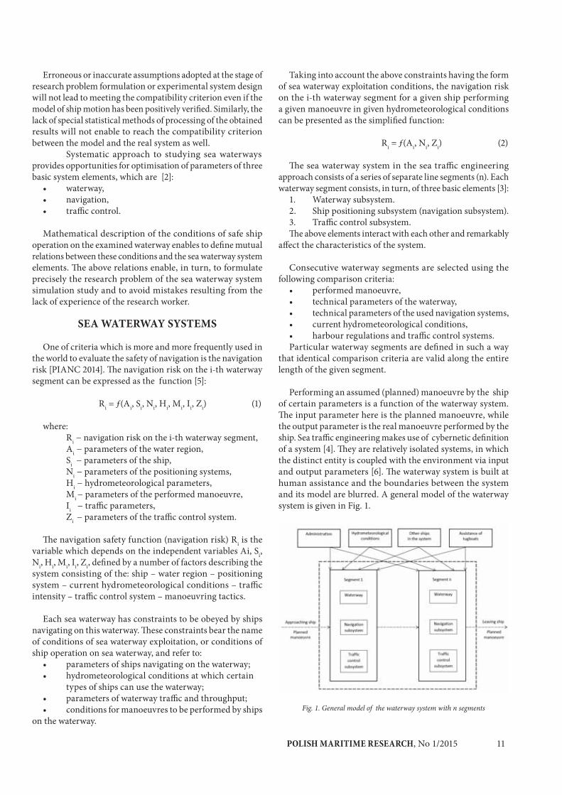
Performing an assumed (planned) manoeuvre by the ship of certain parameters is a function of the waterway system. The input parameter here is the planned manoeuvre, while the output parameter is the real manoeuvre performed by the ship. Sea traffic engineering makes use of cybernetic definition of a system [4]. They are relatively isolated systems, in which the distinct entity is coupled with the environment via input and output parameters [6]. The waterway system is built at human assistance and the boundaries between the system and its model are blurred. A general model of the waterway system is given in Fig. 1.
(1)
(2)
Fig. 1. General model of the waterway system with n segments
POLISH MARITIME RESEARCH, No 1/201512
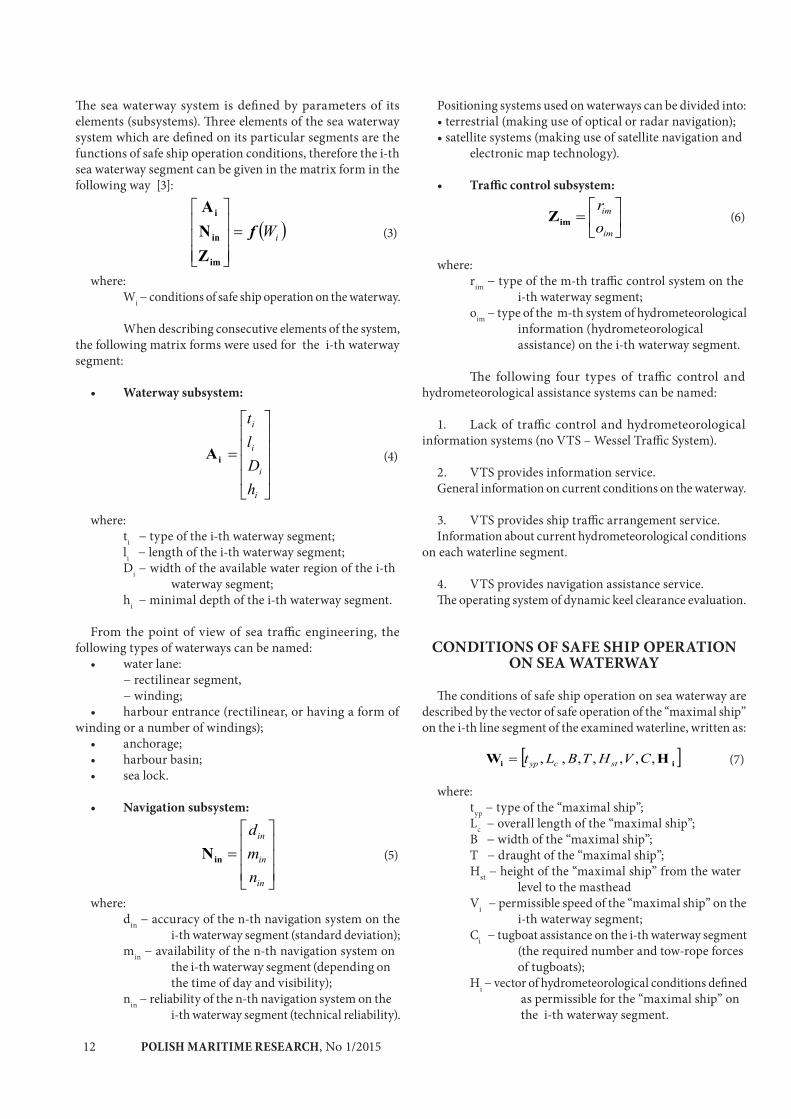
The sea waterway system is defined by parameters of its elements (subsystems). Three elements of the sea waterway system which are defined on its particular segments are the functions of safe ship operation conditions, therefore the i-th sea waterway segment can be given in the matrix form in the following way [3]:
(3)
where: Wi − conditions of safe ship operation on the waterway.
When describing consecutive elements of the system, the following matrix forms were used for the i-th waterway segment:
• Waterway subsystem:
(4)
where: ti − type of the i-th waterway segment; li − length of the i-th waterway segment; Di − width of the available water region of the i-th
waterway segment; hi − minimal depth of the i-th waterway segment.
From the point of view of sea traffic engineering, the following types of waterways can be named:
• water lane: − rectilinear segment, − winding;• harbour entrance (rectilinear, or having a form of
winding or a number of windings);• anchorage;• harbour basin;• sea lock.
• Navigation subsystem:
(5)
where: din − accuracy of the n-th navigation system on the
i-th waterway segment (standard deviation); min − availability of the n-th navigation system on
the i-th waterway segment (depending on the time of day and visibility);
nin − reliability of the n-th navigation system on the i-th waterway segment (technical reliability).
Positioning systems used on waterways can be divided into:• terrestrial (making use of optical or radar navigation);• satellite systems (making use of satellite navigation and
electronic map technology).
• Traffic control subsystem:
(6)
where: rim − type of the m-th traffic control system on the
i-th waterway segment; oim − type of the m-th system of hydrometeorological information (hydrometeorological assistance) on the i-th waterway segment.
The following four types of traffic control and hydrometeorological assistance systems can be named:
1. Lack of traffic control and hydrometeorological information systems (no VTS – Wessel Traffic System).
2. VTS provides information service. General information on current conditions on the waterway.
3. VTS provides ship traffic arrangement service. Information about current hydrometeorological conditions
on each waterline segment.
4. VTS provides navigation assistance service. The operating system of dynamic keel clearance evaluation.
CONDITIONS OF SAFE SHIP OPERATION ON SEA WATERWAY
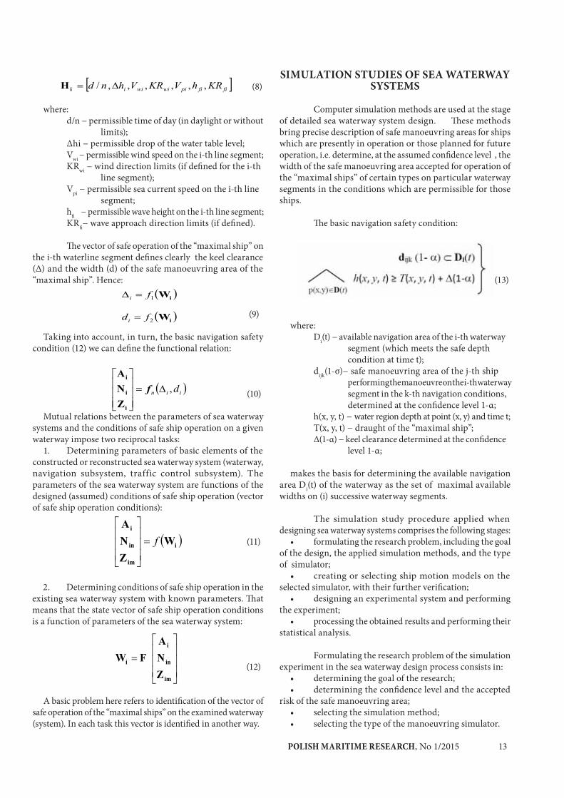
The conditions of safe ship operation on sea waterway are described by the vector of safe operation of the “maximal ship” on the i-th line segment of the examined waterline, written as:
(7)
where: typ − type of the “maximal ship”; Lc − overall length of the “maximal ship”; B − width of the “maximal ship”; T − draught of the “maximal ship”; Hst − height of the “maximal ship” from the water
level to the masthead Vi − permissible speed of the “maximal ship” on the i-th waterway segment; Ci − tugboat assistance on the i-th waterway segment (the required number and tow-rope forces of tugboats); Hi − vector of hydrometeorological conditions defined as permissible for the “maximal ship” on the i-th waterway segment.
POLISH MARITIME RESEARCH, No 1/2015 13
(8)
where: d/n − permissible time of day (in daylight or without limits); Δhi − permissible drop of the water table level; Vwi − permissible wind speed on the i-th line segment; KRwi − wind direction limits (if defined for the i-th line segment); Vpi − permissible sea current speed on the i-th line segment; hfi − permissible wave height on the i-th line segment; KRfi− wave approach direction limits (if defined).
The vector of safe operation of the “maximal ship” on the i-th waterline segment defines clearly the keel clearance (Δ) and the width (d) of the safe manoeuvring area of the “maximal ship”. Hence:
(9)
Taking into account, in turn, the basic navigation safety condition (12) we can define the functional relation:
(10)
Mutual relations between the parameters of sea waterway systems and the conditions of safe ship operation on a given waterway impose two reciprocal tasks:
1. Determining parameters of basic elements of the constructed or reconstructed sea waterway system (waterway, navigation subsystem, traffic control subsystem). The parameters of the sea waterway system are functions of the designed (assumed) conditions of safe ship operation (vector of safe ship operation conditions):
(11)
2. Determining conditions of safe ship operation in the existing sea waterway system with known parameters. That means that the state vector of safe ship operation conditions is a function of parameters of the sea waterway system:
(12)
A basic problem here refers to identification of the vector of safe operation of the “maximal ships” on the examined waterway (system). In each task this vector is identified in another way.
SIMULATION STUDIES OF SEA WATERWAY SYSTEMS
Computer simulation methods are used at the stage of detailed sea waterway system design. These methods bring precise description of safe manoeuvring areas for ships which are presently in operation or those planned for future operation, i.e. determine, at the assumed confidence level , the width of the safe manoeuvring area accepted for operation of the “maximal ships” of certain types on particular waterway segments in the conditions which are permissible for those ships.
The basic navigation safety condition:
where: Di(t) − available navigation area of the i-th waterway
segment (which meets the safe depth condition at time t);
dijk(1-σ)− safe manoeuvring area of the j-th ship performing the manoeuvre on the i-th waterway segment in the k-th navigation conditions, determined at the confidence level 1-α;
h(x, y, t) − water region depth at point (x, y) and time t; T(x, y, t) − draught of the “maximal ship”; Δ(1-α) − keel clearance determined at the confidence
level 1-α;
makes the basis for determining the available navigation area Di(t) of the waterway as the set of maximal available widths on (i) successive waterway segments.
The simulation study procedure applied when designing sea waterway systems comprises the following stages:
• formulating the research problem, including the goal of the design, the applied simulation methods, and the type of simulator;
• creating or selecting ship motion models on the selected simulator, with their further verification;
• designing an experimental system and performing the experiment;
• processing the obtained results and performing their statistical analysis.
Formulating the research problem of the simulation experiment in the sea waterway design process consists in:
• determining the goal of the research;• determining the confidence level and the accepted
risk of the safe manoeuvring area;• selecting the simulation method;• selecting the type of the manoeuvring simulator.
(13)
POLISH MARITIME RESEARCH, No 1/201514
In the simulation studies used at the stage of detailed sea waterway design, use is made of the results of preliminary waterway design to determine:
• parameters of basic waterway system elements which were determined using empirical methods at the preliminary design stage:
(14)
• the verified matrix of conditions of safe ship operation on the designed waterway Mi:
(15)
where: Wij − vector of safe operation conditions for the
“maximal ship” of j-th type in operation on the examined waterway.
• the vector of safe operation conditions for the “maximal ship” which requires the largest width di max of the save manoeuvring area and which was used at the preliminary stage for determining the parameters of the waterway elements:
(16)
If the comparable widths of the safe manoeuvring areas were calculated for more “maximal ships” than one at the preliminary design stage, all these ships are qualified for the simulation study. A case can occur when the simulation study is performed for a number of models having the following safe operation vectors:
(17)
The “maximal ships” which were qualified for the simulation study bear the name of “characteristic ships” of the examined waterway. The above data is used for selecting the method of simulation study and the type of the used simulators.
At present, the following computer simulation methods are used at the waterway design stage:
1. Method RTS (Real Time Simulation) of ship motion which makes use of non-autonomous models.
2. Method FTS (Fast Time Simulation) of ship motion which makes use of autonomous models.
3. Method which generalises the results of simulation studies.
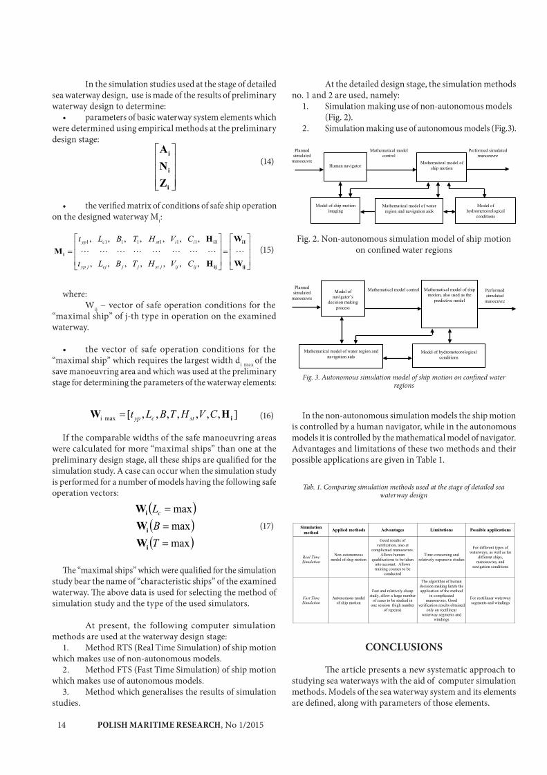
At the detailed design stage, the simulation methods no. 1 and 2 are used, namely:
1. Simulation making use of non-autonomous models (Fig. 2).
2. Simulation making use of autonomous models (Fig.3).
Fig. 2. Non-autonomous simulation model of ship motion on confined water regions
Fig. 3. Autonomous simulation model of ship motion on confined water regions
In the non-autonomous simulation models the ship motion is controlled by a human navigator, while in the autonomous models it is controlled by the mathematical model of navigator. Advantages and limitations of these two methods and their possible applications are given in Table 1.
Tab. 1. Comparing simulation methods used at the stage of detailed sea waterway design
CONCLUSIONS
The article presents a new systematic approach to studying sea waterways with the aid of computer simulation methods. Models of the sea waterway system and its elements are defined, along with parameters of those elements.

POLISH MARITIME RESEARCH, No 1/2015 15
Systematic approach to sea waterway studies makes it possible to optimise three basic elements of the system, which are:
• waterway,• navigation,• traffic control.
Conditions of safe ship operation in the sea waterway system are described. Relations between the system elements and the conditions of safe ship operation in this system are defined. Based on these relations, principles of clear formulation of research problems in simulation studies of sea waterways are worked out.
The simulation studies are used at the stage of detailed sea waterway system design. Correct formulation of their research problem, followed by proper design of the experimental system and processing of the obtained results, is of high importance, as it enables to obtain reliable results and avoid errors in designing sea waterway systems.
The here described method of simulation studies of sea waterway systems was used in re-designing the waterway to the Świnoujście harbour, which was modernised to take into account requirements of LNG carriers of Q-flex type, and in modernisation of the Świnoujście-Szczecin waterway (depth increase to 12,5 m).
BIBLIOGRAPHY
1. Gucma M. (2007): Multi-factor Variance Analysis Method for Optimization of Pilot System Interface. Proceeding of the XII International Scientific and Technical Conference on Marine Traffic Engineering. Świnoujście, 20-23.11.2007.
2. Gucma S. (2013a): Optimisation of sea waterway system parameters in marine traffic engineering. Journal of KONBIN, No 2 (26) 2013, Wydawnictwo ITWL, Warszawa.
3. Gucma S. (2013b): Conditions of safe ship operation in sea waterway systems (in Polish). Proc. of the International Scientific Conference on “Sea Traffic Engineering”. Świnoujście, 16-18.10.2013.
4. Gucma S., Gucma L., Zalewski P. (2008): Simulation methods in sea traffic engineering (in Polish). Wydawnictwo Naukowe Akademii Morskiej w Szczecinie, Szczecin 2008.
5. Gucma S., Ślączka W., Zalewski P. (2013): Parameters of water lanes and navigation systems determined with the aid of navigation safety criterion (in Polish). Wydawnictwo Naukowe Akademii Morskiej w Szczecinie, Szczecin 2013.
6. Gutenbaum J. (2003): Mathematical modelling of systems (in Polish). Akademicka Oficyna Wydawnicza EXIT, Warszawa 2003.
7. PIANC (2014): Report No 121-2014. Harbour approach channels design guidelines. PIANC Secrétariat Général, Bruxelles.
CONTACT WITH THE AUTOR
Stanisław Gucma
Marine Traffic Engineering CentreFaculty of Navigation
Maritime University of Szczecin 1-2 Waly Chrobrego Str.
70-500 SzczecinPOLAND
e-mail: [email protected]
POLISH MARITIME RESEARCH, No 1/201516
POLISH MARITIME RESEARCH 1(85) 2015 Vol. 22; pp. 16-2110.1515/pomr-2015-0003
THE DESIGN OF SHIP AUTOPILOT BY APPLYING OBSERVER - BASED FEEDBACK LINEARIZATION
Zenon Zwierzewicz, Prof.Maritime University of Szczecin, Poland
ABSTRACT
The paper considers the problem of ship autopilot design based on Bech’s model of the vessel. Since the model is highly nonlinear and some of the state vector coordinates are unavailable, the control system synthesis is performed by means of an output feedback linearization method combined with a nonlinear observer. The asymptotic stability of the overall system has been proven, including the asymptotic stability of the system internal dynamics. The performed simulations of the ship course-changing process have confirmed a high performance of the proposed controller. It has been emphasized that for its practical usability the system robustification is necessary.
Keywords: ship autopilot design, feedback linearization, nonlinear observer
INTRODUCTION
The course-keeping and course-changing problems are still vital issues during the ship handling process. In real circumstances, we have to cope with the presence of different kinds of uncertainty, such as: inaccuracies in the system model, the presence of random processes’ statistics, such as winds, waves, currents, and other exogenous effects, the different sailing conditions such as speed, loading conditions, trim etc, as well as varied sailing routes - in open sea (deep water) or coastal (shallow waters) with a possible change in the under keel clearance.
This necessitates, when designing a vessel control system, employment of the techniques that take into account the process nonlinear effects as well as the consideration of the ship model parametrical uncertainty.
The most common methods for nonlinear systems control, intensively developed during last two decades, are feedback linearization and back-stepping. Each of them has its advantages and drawbacks.
The back-stepping procedure requires, for instance, the systems with special triangular structure (pure feedback form) and suffers from inherent ‘explosion of terms’ issue [7].
The feedback (or exact) linearization, in turn, has to satisfy the so-called matching condition [6], which implies that the uncertainty terms appear in the same equations as the control inputs u, and as a result they can be handled by the controller.
Further issues that concern the above mentioned nonlinear control techniques relate to the model parametric uncertainty problem, as well as to the question of accessibility of the system state, which leads to the subsequent task of observer design.
Applying these techniques to the systems with uncertain parameters leads to the inexact compensation of the model
non-linearities, which requires employing an adaptive or robust control methods during the controller design.
The main objective of the paper is to propose a ship course-keeping controller design based on highly nonlinear Bech’s ship model[4]. Because of the general model structure that excludes the use of the back-stepping method, we apply the feedback linearization combined with a nonlinear observer. It has been proven that the overall linearized system as well as its internal (zero) dynamics [6, 13] are asymptotically stable.
The herein proposed design assumes the full knowledge about the model parameters. However, knowing that for its practical usability the system parametrical uncertainties have to be considered, the paper is the first part of a larger project. The adaptive version of this proposal will be presented in its second part.
The paper is divided into five sections and ends with conclusions. The second section presents the models of the ship and steering gear, including model parameters. In the third section the controller design by using output feedback linearization is described along with an analysis of system internal dynamics . In the fourth section the reduced - order nonlinear observer is derived and the stability of the overall system is proven. The last, fifth section includes a short description of simulation tests and their results.
MODELS OF THE SHIP AND ITS STEERING GEAR
At first we introduce the following Bech’s ship dynamic model [4,1,15]
(1)
POLISH MARITIME RESEARCH, No 1/2015 17
where ψ(t) - ship heading - the controlled variable ψ(t) = r - angular velocity (rate of turn)δ(t) - rudder deflection - a control variable
Function HB (ψ) describes a nonlinear ship maneuvering characteristic. In the steady state when ψ(t) = ψ(t) = δ(t) = 0, it follows that δ = HB(ψ) , which is the formula describing Bech’s reversed spiral characteristic. A good approximation for the non-linear function HB(ψ) has appeared to be :
(2)
A single screw propeller or asymmetry in the hull will cause a non-zero value of b0. Similarly, symmetry in the hull implies that b2 = 0 . Course instability results in a negative value of b1. Since a constant rudder angle is required to compensate for constant steady-state wind and current disturbances, the bias term b0 is frequently taken as null, being conveniently treated as an additional rudder offset.
As the ship model nominal parameters, the dynamic maneuvering parameters of marine class vessel [3] are adopted: K = 11,1 1/min, T1 = 1,967 min, T2 = 0,13 min, T3 = 0,308 min, b3 = 0,4 min3/rad2, b2 = 0 min2/rad, b1 = 2 min, b0 = 0rad.
The ship has the following characteristics: displacement: 18541 m3, draft: 8.23 m, length overall: 171,8 m, length between perpendiculars: 160,93 m, maximum beam: 23,17m, one propeller, and maximum speed: 15 knots. The maximum rudder angle and maximum rate of turn are: 35 deg = 0,61 rad and 1 deg/s = 1,047 rad/min, respectively.
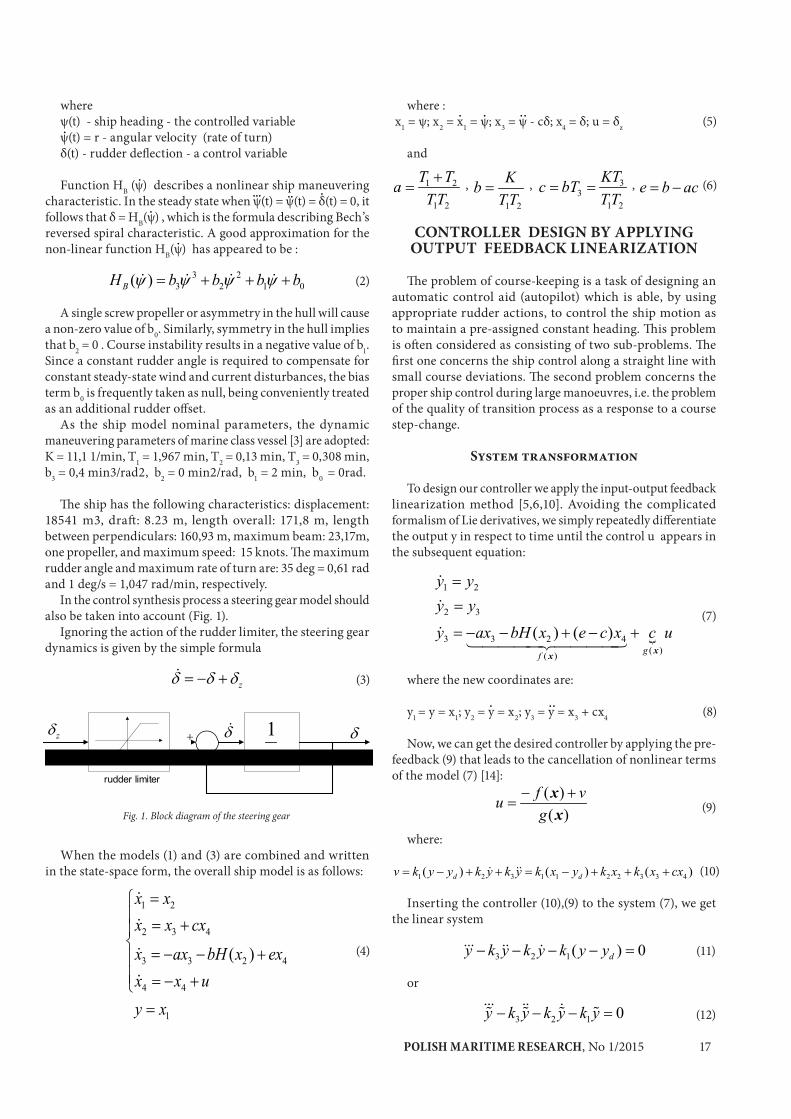
In the control synthesis process a steering gear model should also be taken into account (Fig. 1).
Ignoring the action of the rudder limiter, the steering gear dynamics is given by the simple formula
(3)
Fig. 1. Block diagram of the steering gear
When the models (1) and (3) are combined and written in the state-space form, the overall ship model is as follows:
(4)
where : x1 = ψ; x2 = x1 = ψ; x3 = ψ - cδ; x4 = δ; u = δz
and
,, ,
(5)
(6)
CONTROLLER DESIGN BY APPLYING OUTPUT FEEDBACK LINEARIZATION
The problem of course-keeping is a task of designing an automatic control aid (autopilot) which is able, by using appropriate rudder actions, to control the ship motion as to maintain a pre-assigned constant heading. This problem is often considered as consisting of two sub-problems. The first one concerns the ship control along a straight line with small course deviations. The second problem concerns the proper ship control during large manoeuvres, i.e. the problem of the quality of transition process as a response to a course step-change.
System transformation
To design our controller we apply the input-output feedback linearization method [5,6,10]. Avoiding the complicated formalism of Lie derivatives, we simply repeatedly differentiate the output y in respect to time until the control u appears in the subsequent equation:
(7)
where the new coordinates are:
Now, we can get the desired controller by applying the pre-feedback (9) that leads to the cancellation of nonlinear terms of the model (7) [14]:
y1 = y = x1; y2 = y = x2; y3 = y = x3 + cx4 (8)
(9)
where:
(10)
Inserting the controller (10),(9) to the system (7), we get the linear system
(11)
or
(12)
POLISH MARITIME RESEARCH, No 1/201518
where:
This system is stable by virtue of the proper choice of coefficients, which can be done by, e.g., the pole placement technique.
Internal dynamics analysisBy means of input-output linearization, the dynamics of
nonlinear system is decomposed into an external (input-output) dynamics part and an internal (‘unobservable’) part.
After the partial coordinate transformation (8), we have got a new system (7) of third order which represents the external dynamics. Because the original system (4) is of fourth degree here, there must be an additional dynamics [6] (internal or zero dynamics) described by a subsequent equation.
It is very important, during the controller design, to find out whether the zero dynamics is stable, otherwise this approach does not produce a control law of any practical use. This internal dynamics can be found by completing the coordinate transform, which leads to a partial differential equation (PDE).
In order to avoid coping with a PDE, which is rather complicated, we use a simplified method. To this end it is useful to know that the zero dynamics can be characterized in the original coordinates [6]. Noting that:
(13)
we see that if the output is identical to zero, the solution of the system equations must be confined to the smooth surface (manifold):
(14)
and the input must be:
(15)
Now, inserting the state coordinates defined by (14) and the control u of (15) to the original system (4), we get the equation describing the zero dynamics in the form
(16)
As the parameters b and c are positive, we have proved that the zero dynamics is asymptotically stable.
NONLINEAR OBSERVER DESIGN
For a practical application of formula (9), we have to measure the state vector x = [x1 x2 x3 x4]T = [ψ r x3 δ]T. As the access to the variable x3 can be problematic, a state observer must be used in order to overcome this difficulty.
We propose the following reduced-order, nonlinear observer:
(17)
where y = x2 = r is assumed the measurable signal and the gain matrix L = [l1, l2]T should be selected as to get the observation error (compare (23)) exponentially converging to the origin.
By means of (17) we can get the estimate x3.The question is if putting into the controller (10) the estimate
x3 (from the observer (17)) , instead of the original value x3, does not affect the system stability.
To prove that the overall system will be still stable, we perform the following reasoning.
Let us first re-write the formula (11) in the form:
(18)
Knowing now that instead of x3 we have in fact x3, we re-write (18) as follows:
(19)
Now adding to and subtracting from the left side of (19) the term k3x3 we get:
(20)
Denoting the estimation error as x3 = (x3 - x3) we finally get:
(21)
or(22)
where y = y - yd.
By subtracting from second and third equations of the system (4) the observer equations (17) we get the system describing observation error:
(23)
Treating now x3 as an output of the system (23) and knowing that it at the same time is the input to the system (22), we have a cascaded inter-connection of two asymptotically stable, linear time-invariant systems, which makes the overall system (Fig. 2) also asymptotically stable.
POLISH MARITIME RESEARCH, No 1/2015 19
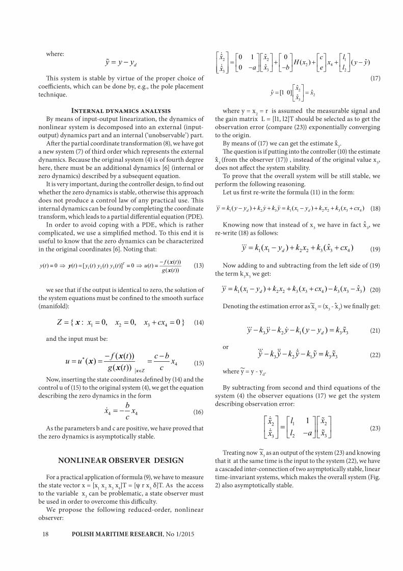
Fig. 2. Block diagram of the system (4),(9),(17)
COURSE-CHANGING PROCESS SIMULATIONS
The standard method of assessing the control system quality is based on analysis of the transition process as a response to the step input. Thus, in the following simulations we will test the ship behaviour after step-change of the course set-point for directionally stable or unstable ship.
The following charts show the situations where the ship is moving ahead at a steady speed (0.25 nm/min) along a straight line, and then we apply a 30-degree step course change command.
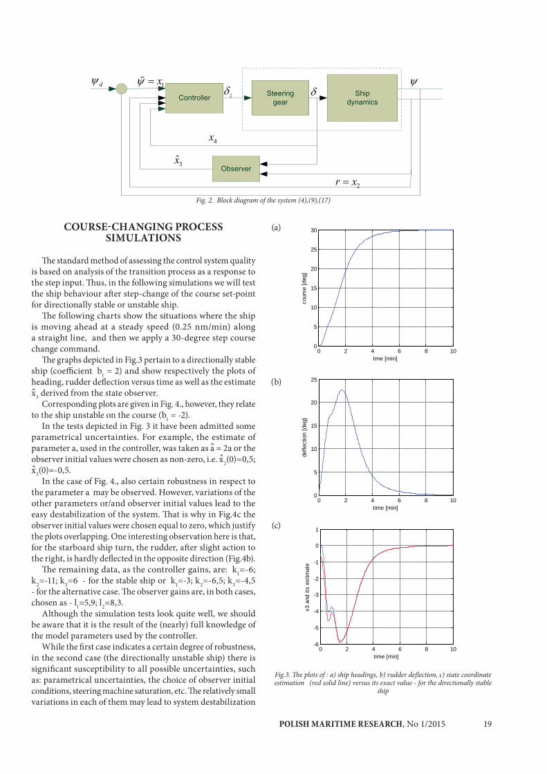
The graphs depicted in Fig.3 pertain to a directionally stable ship (coefficient b1 = 2) and show respectively the plots of heading, rudder deflection versus time as well as the estimate x3 derived from the state observer.
Corresponding plots are given in Fig. 4., however, they relate to the ship unstable on the course (b1 = -2).
Fig.3. The plots of : a) ship headings, b) rudder deflection, c) state coordinate estimation (red solid line) versus its exact value - for the directionally stable
ship
In the tests depicted in Fig. 3 it have been admitted some parametrical uncertainties. For example, the estimate of parameter a, used in the controller, was taken as a = 2a or the observer initial values were chosen as non-zero, i.e. x2(0)=0,5; x3(0)=-0,5.
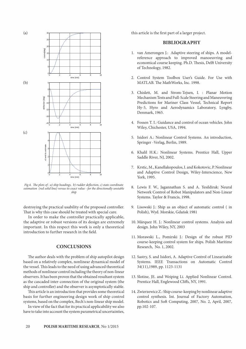
In the case of Fig. 4., also certain robustness in respect to the parameter a may be observed. However, variations of the other parameters or/and observer initial values lead to the easy destabilization of the system. That is why in Fig.4c the observer initial values were chosen equal to zero, which justify the plots overlapping. One interesting observation here is that, for the starboard ship turn, the rudder, after slight action to the right, is hardly deflected in the opposite direction (Fig.4b).
(a)
(b)
(c)
The remaining data, as the controller gains, are: k1=-6; k2=-11; k3=6 - for the stable ship or k1=-3; k2=-6,5; k3=-4,5 - for the alternative case. The observer gains are, in both cases, chosen as - l1=5,9; l2=8,3.
Although the simulation tests look quite well, we should be aware that it is the result of the (nearly) full knowledge of the model parameters used by the controller.
While the first case indicates a certain degree of robustness, in the second case (the directionally unstable ship) there is significant susceptibility to all possible uncertainties, such as: parametrical uncertainties, the choice of observer initial conditions, steering machine saturation, etc. The relatively small variations in each of them may lead to system destabilization
0 2 4 6 8 100
5
10
15
20
25
30
tme [min]
cour
se [d
eg]
0 2 4 6 8 100
5
10
15
20
25
time [min]
defle
ctio
n [d
eg]
0 2 4 6 8 10-6
-5
-4
-3
-2
-1
0
1
time [min]
x3 a
nd it
s es
timat
e
POLISH MARITIME RESEARCH, No 1/201520
Fig.4. The plots of : a) ship headings, b) rudder deflection, c) state coordinate estimation (red solid line) versus its exact value - for the directionally unstable
ship
(c)
(b)
(a)
destroying the practical usability of the proposed controller. That is why this case should be treated with special care.
In order to make the controller practically applicable, the adaptive or robust versions of its design are extremely important. In this respect this work is only a theoretical introduction to further research in the field.
CONCLUSIONS
The author deals with the problem of ship autopilot design based on a relatively complex, nonlinear dynamical model of the vessel. This leads to the need of using advanced theoretical methods of nonlinear control including the theory of non-linear observers. It has been proven that the obtained resultant system as the cascaded inter-connection of the original system (the ship and controller) and the observer is asymptotically stable.
This article is an introduction that provides some theoretical basis for further engineering design work of ship control systems, based on the complex, Bech’s non-linear ship model.
In view of the fact that for its practical applicability we also have to take into account the system parametrical uncertainties,
this article is the first part of a larger project.
BIBLIOGRAPHY
1. van Amerongen J.: Adaptive steering of ships. A model-reference approach to improved manoeuvring and economical course keeping. Ph.D. Thesis, Delft University of Technology, 1982.
2. Control System Toolbox User’s Guide. For Use with MATLAB. The MathWorks, Inc. 1998.
3. Chislett, M. and Strom-Tejsen, I. : Planar Motion Mechanism Tests and Full-Scale Steering and Maneuvering Predictions for Mariner Class Vessel, Technical Report Hy-5, Hyro and Aerodynamics Laboratory, Lyngby, Denmark, 1965.
4. Fossen T. I.: Guidance and control of ocean vehicles. John Wiley, Chichester, USA, 1994.
5. Isidori A.: Nonlinear Control Systems. An introduction, Springer -Verlag, Berlin, 1989.
6. Khalil H.K.: Nonlinear Systems. Prentice Hall, Upper Saddle River, NJ, 2002.
7. Krstic, M., Kanellakopoulos, I. and Kokotovic, P. Nonlinear and Adaptive Control Design, Wiley-Interscience, New York, 1995.
8. Lewis F. W., Jagannathan S. and A. Yesildirak: Neural Network Control of Robot Manipulators and Non-Linear Systems. Taylor & Francis, 1998.
9. Lisowski J.: Ship as an object of automatic control ( in Polish), Wyd. Morskie, Gdańsk 1981
10. Márquez H. J.: Nonlinear control systems. Analysis and design. John Wiley, NY, 2003
11. Morawski L., Pomirski J.: Design of the robust PID course-keeping control system for ships. Polish Maritime Research, No. 1, 2002.
12. Sastry, S. and Isidori, A. Adaptive Control of Linearizable Systems. IEEE Transactions on Automatic Control 34(11),1989, pp. 1123-1131
13. Slotine, JE. and Weiping Li. Applied Nonlinear Control. Prentice Hall, Englewood Cliffs, NY, 1991.
14. Zwierzewicz Z.: Ship course-keeping by nonlinear adaptive control synthesis. Int. Journal of Factory Automation, Robotics and Soft Computing, 2007, No. 2, April, 2007, pp.102-107.
0 2 4 6 8 100
5
10
15
20
25
30
time [min]
cour
se[d
eg]
0 2 4 6 8 10-25
-20
-15
-10
-5
0
5
time [min]
defle
ctio
n [d
eg]
0 2 4 6 8 100
1
2
3
4
5
time [min]
x3
and
its e
stim
ate

POLISH MARITIME RESEARCH, No 1/2015 21
15. Zwierzewicz Z.: Methods and algorithms of ship automatic control systems (in Polish). Scientific publishing house of Szczecin Maritime University, Szczecin 2012.
CONTACT WITHE THE AUTOR
Zenon Zwierzewicz
Maritime University of Szczecin1-2 Wały Chrobrego St.70-500 Szczecin, Poland
POLISH MARITIME RESEARCH, No 1/201522
POLISH MARITIME RESEARCH 1(85) 2015 Vol. 22; pp. 22-2710.1515/pomr-2015-0004
TEST STUDIES OF THE RESISTANCE AND SEAKEEPING PERFORMANCE OF A TRIMARAN PLANING HULL
Weijia Ma, Ph.D.Hanbing Sun, Ph.D.Huawei Sun, Ph.D.Jin Zou, Prof.Jiayuan Zhuang, Ph.D.
ABSTRACT
Towing tank tests in calm water were performed on a trimaran planing hull to verify its navigational properties with different displacements and centres of gravity, as well as to assess the effects of air jets and bilge keels on the hull’s planing capabilities, and to increase the longitudinal stability of the hull. Hydrostatic roll tests, zero speed tests, and sea trials in the presence of regular waves were conducted to investigate the hull’s seakeeping ability. The test results indicate that the influence of the location of the centre of gravity on the hull resistance is similar to that of a normal trimaran planing hull; namely, moving the centre of gravity backward will reduce the resistance but lower the stability. Bilge keels improve the longitudinal stability but slightly affect the resistance, and the presence of air jets in the hull’s channels decreases the trim angle and increases heaving but has little effect on the resistance. Frequent small-angle rolling occurs in waves. The heaving and pitching motions peak at the encounter frequency of , and the peaks increase with velocity and move towards greater encounter frequencies. When the encounter frequency exceeds, the hull motion decreases, which leads to changes in the navigation speed and frequency.
Keywords: trimaran planing hull; appendix; resistance; seakeeping; model test
INTRODUCTION
Trimaran planing hulls exhibit excellent navigational performance. These hulls are composed of a main hull and two auxiliary appendages. A trimaran planing hull combines the advantages of a normal planing hull, a high-speed multihull vessel, and a ship that uses a gas layer to reduce the resistance. It has good hydrodynamic and aerodynamic performance characteristics and will plane at normal speeds. Due to their high speed and good adaption to different sea states, trimaran planing hulls have both military and civil applications.
The effects of different positions of the centre of gravity, steps, air injection quantities, and attempts to control the resistance of planing crafts have been studied extensively [1-4]. The resistance characteristics of a planing hull with and without spray strips under various displacements and centres of gravity have been investigated, and model tests have been used to explore the influence of steps on the navigation performance and resistance of trimaran planing hulls. The results of these studies provide guidance for designing hulls which will reveal the assumed features. Numerous model tests of planing vessels have been carried out in waves, including tests of prismatic planing hulls in regular and irregular waves [5-6]. In addition, experiments have been conducted on the longitudinal movement of high-speed planing crafts [7] and deep-V planing hulls [8] in the presence of regular waves.
To reduce the resistance of trimaran planing hulls, the present study examines selected additions to the model vessel. Two rows of air holes along the top of the channels on the back of the planing hulls were designed to investigate the influence of air jets on the fluid performance inside the channels, and a bilge keel was set above the bevel line of the main hull. Because of the complexity of the seakeeping performance of trimaran planing hulls, several model tests were performed in this study, including roll decay tests in calm water, zero speed tests, and sea trials in the presence of regular waves.
RESISTANCE TESTS OF THE TRIMARAN PLANING HULL
Test model
The ship model is made of fibre-reinforced plastic (FRP) and is shown in Fig. 1. The principal dimensions are shown in Tab. 1.
The main purposes of the tests were: (1) to verify navigation properties and resistance characteristics of the designed trimaran planing hull with different displacements and centres of gravity, (2) to assess the effect of the air jets in the channels and the bilge keels on the hull’s planing capabilities, and (3) to explore measures of increasing the longitudinal stability.
POLISH MARITIME RESEARCH, No 1/2015 23
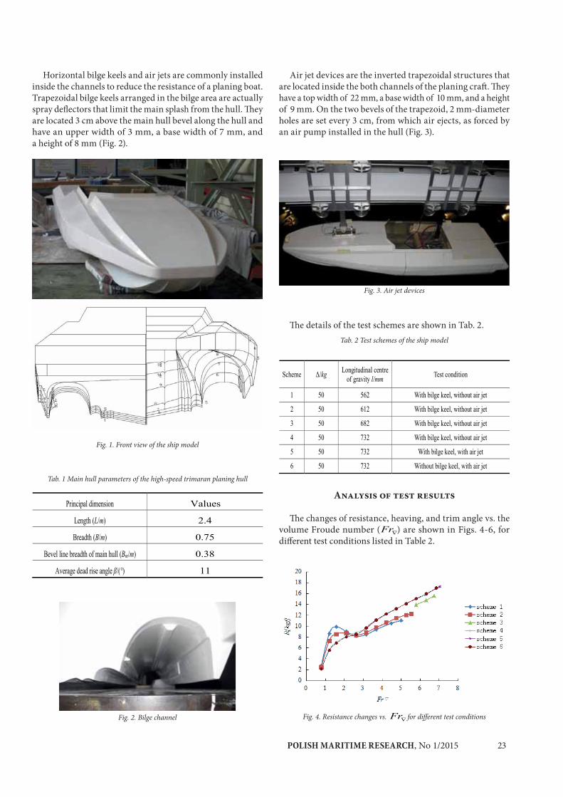
Horizontal bilge keels and air jets are commonly installed inside the channels to reduce the resistance of a planing boat. Trapezoidal bilge keels arranged in the bilge area are actually spray deflectors that limit the main splash from the hull. They are located 3 cm above the main hull bevel along the hull and have an upper width of 3 mm, a base width of 7 mm, and a height of 8 mm (Fig. 2).
Fig. 1. Front view of the ship model
Tab. 1 Main hull parameters of the high-speed trimaran planing hull
Fig. 2. Bilge channel
Air jet devices are the inverted trapezoidal structures that are located inside the both channels of the planing craft. They have a top width of 22 mm, a base width of 10 mm, and a height of 9 mm. On the two bevels of the trapezoid, 2 mm-diameter holes are set every 3 cm, from which air ejects, as forced by an air pump installed in the hull (Fig. 3).
Fig. 3. Air jet devices
The details of the test schemes are shown in Tab. 2.Tab. 2 Test schemes of the ship model
Analysis of test results
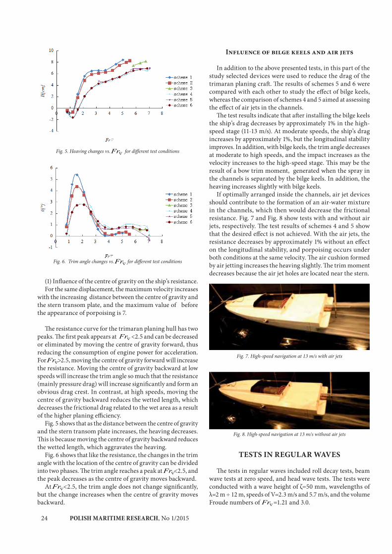
The changes of resistance, heaving, and trim angle vs. the volume Froude number ( ) are shown in Figs. 4-6, for different test conditions listed in Table 2.
Fig. 4. Resistance changes vs. for different test conditions
POLISH MARITIME RESEARCH, No 1/201524
Fig. 5. Heaving changes vs. for different test conditions
Fig. 6. Trim angle changes vs. for different test conditions
(1) Influence of the centre of gravity on the ship’s resistance.For the same displacement, the maximum velocity increases
with the increasing distance between the centre of gravity and the stern transom plate, and the maximum value of before the appearance of porpoising is 7.
The resistance curve for the trimaran planing hull has two peaks. The first peak appears at <2.5 and can be decreased or eliminated by moving the centre of gravity forward, thus reducing the consumption of engine power for acceleration. For >2.5, moving the centre of gravity forward will increase the resistance. Moving the centre of gravity backward at low speeds will increase the trim angle so much that the resistance (mainly pressure drag) will increase significantly and form an obvious drag crest. In contrast, at high speeds, moving the centre of gravity backward reduces the wetted length, which decreases the frictional drag related to the wet area as a result of the higher planing efficiency.
Fig. 5 shows that as the distance between the centre of gravity and the stern transom plate increases, the heaving decreases. This is because moving the centre of gravity backward reduces the wetted length, which aggravates the heaving.
Fig. 6 shows that like the resistance, the changes in the trim angle with the location of the centre of gravity can be divided into two phases. The trim angle reaches a peak at <2.5, and the peak decreases as the centre of gravity moves backward.
At <2.5, the trim angle does not change significantly, but the change increases when the centre of gravity moves backward.
Influence of bilge keels and air jets
In addition to the above presented tests, in this part of the study selected devices were used to reduce the drag of the trimaran planing craft. The results of schemes 5 and 6 were compared with each other to study the effect of bilge keels, whereas the comparison of schemes 4 and 5 aimed at assessing the effect of air jets in the channels.
The test results indicate that after installing the bilge keels the ship’s drag decreases by approximately 1% in the high-speed stage (11-13 m/s). At moderate speeds, the ship’s drag increases by approximately 1%, but the longitudinal stability improves. In addition, with bilge keels, the trim angle decreases at moderate to high speeds, and the impact increases as the velocity increases to the high-speed stage. This may be the result of a bow trim moment, generated when the spray in the channels is separated by the bilge keels. In addition, the heaving increases slightly with bilge keels.
If optimally arranged inside the channels, air jet devices should contribute to the formation of an air-water mixture in the channels, which then would decrease the frictional resistance. Fig. 7 and Fig. 8 show tests with and without air jets, respectively. The test results of schemes 4 and 5 show that the desired effect is not achieved. With the air jets, the resistance decreases by approximately 1% without an effect on the longitudinal stability, and porpoising occurs under both conditions at the same velocity. The air cushion formed by air jetting increases the heaving slightly. The trim moment decreases because the air jet holes are located near the stern.
Fig. 7. High-speed navigation at 13 m/s with air jets
Fig. 8. High-speed navigation at 13 m/s without air jets
TESTS IN REGULAR WAVES
The tests in regular waves included roll decay tests, beam wave tests at zero speed, and head wave tests. The tests were conducted with a wave height of ζ=50 mm, wavelengths of λ=2 m ÷ 12 m, speeds of V=2.3 m/s and 5.7 m/s, and the volume Froude numbers of =1.21 and 3.0.
POLISH MARITIME RESEARCH, No 1/2015 25
Results and analysis of roll decay tests
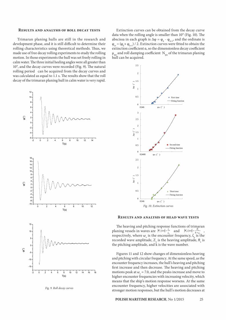
Trimaran planing hulls are still in the research and development phase, and it is still difficult to determine their rolling characteristics using theoretical methods. Thus, we made use of free decay rolling experiments to study the rolling motion. In those experiments the hull was set freely rolling in calm water. The three initial heeling angles were all greater than 10°, and the decay curves were recorded (Fig. 9). The natural rolling period can be acquired from the decay curves and was calculated as equal to 1.1 s. The results show that the roll decay of the trimaran planing hull in calm water is very rapid.
Fig. 9. Roll decay curves
Extinction curves can be obtained from the decay curve data when the rolling angle is smaller than 10° (Fig. 10). The abscissa in each graph is Δφ = φk - φk+1, and the ordinate is φm = (φk+ φk+1) / 2. Extinction curves were fitted to obtain the extinction coefficient α, so the dimensionless decay coefficient μφφ and roll damping coefficient Nφφ of the trimaran planing hull can be acquired.
0
0.5
1
1.5
2
2.5
0246
()
m ( )
First timeFitting function
0
0.5
1
1.5
2
2.5
3
02468
()
m ( )
Second timeFitting function
0
0.5
1
1.5
2
2.5
0246
()
m ( )
Third timeFitting function
Fig. 10. Extinction curves
Results and analysis of head wave tests
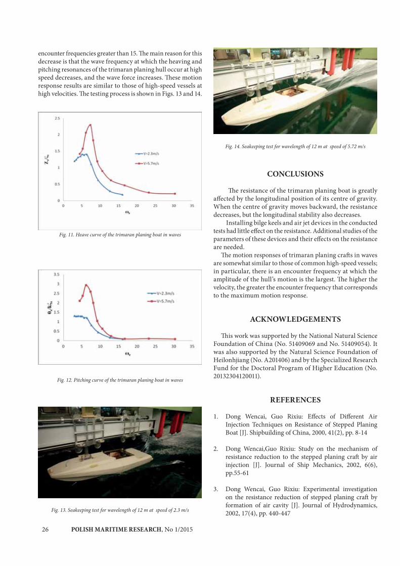
The heaving and pitching response functions of trimaran planing vessels in waves are and , respectively, where ωe is the encounter frequency, ζa is the recorded wave amplitude, Za is the heaving amplitude, θa is the pitching amplitude, and k is the wave number.
Figures 11 and 12 show changes of dimensionless heaving and pitching with circular frequency. At the same speed, as the encounter frequency increases, the hull’s heaving and pitching first increase and then decrease. The heaving and pitching motions peak at ωe ≈ 7.0, and the peaks increase and move to higher encounter frequencies with increasing velocity, which means that the ship’s motion response worsens. At the same encounter frequency, higher velocities are associated with stronger motion responses, but the hull’s motion decreases at
POLISH MARITIME RESEARCH, No 1/201526
encounter frequencies greater than 15. The main reason for this decrease is that the wave frequency at which the heaving and pitching resonances of the trimaran planing hull occur at high speed decreases, and the wave force increases. These motion response results are similar to those of high-speed vessels at high velocities. The testing process is shown in Figs. 13 and 14.
Fig. 11. Heave curve of the trimaran planing boat in waves
Fig. 12. Pitching curve of the trimaran planing boat in waves
Fig. 13. Seakeeping test for wavelength of 12 m at speed of 2.3 m/s
Fig. 14. Seakeeping test for wavelength of 12 m at speed of 5.72 m/s
CONCLUSIONS
The resistance of the trimaran planing boat is greatly affected by the longitudinal position of its centre of gravity. When the centre of gravity moves backward, the resistance decreases, but the longitudinal stability also decreases.
Installing bilge keels and air jet devices in the conducted tests had little effect on the resistance. Additional studies of the parameters of these devices and their effects on the resistance are needed.
The motion responses of trimaran planing crafts in waves are somewhat similar to those of common high-speed vessels; in particular, there is an encounter frequency at which the amplitude of the hull’s motion is the largest. The higher the velocity, the greater the encounter frequency that corresponds to the maximum motion response.
ACKNOWLEDGEMENTS
This work was supported by the National Natural Science Foundation of China (No. 51409069 and No. 51409054). It was also supported by the Natural Science Foundation of Heilonhjiang (No. A201406) and by the Specialized Research Fund for the Doctoral Program of Higher Education (No. 20132304120011).
REFERENCES
1. Dong Wencai, Guo Rixiu: Effects of Different Air Injection Techniques on Resistance of Stepped Planing Boat [J]. Shipbuilding of China, 2000, 41(2), pp. 8-14
2. Dong Wencai,Guo Rixiu: Study on the mechanism of resistance reduction to the stepped planing craft by air injection [J]. Journal of Ship Mechanics, 2002, 6(6), pp.55-61
3. Dong Wencai, Guo Rixiu: Experimental investigation on the resistance reduction of stepped planing craft by formation of air cavity [J]. Journal of Hydrodynamics, 2002, 17(4), pp. 440-447

POLISH MARITIME RESEARCH, No 1/2015 27
4. Xia Xiang: Matching performance of propulsion system for hypervelocity step planing boat [J]. Chinese Journal of Ship Research, 2008, 3(2), pp. 39-42
5. Fridsma, G.: A Systematic Study of the Rough-Water Performance of Planing Boat, Davidson Laboratory, Stevens Institute, Report R-1275, Nov, 1969
6. Fridsma, G.: A Systematic Study of the Rough-Water Performance of Planing Boat-Irregular Waves, Part II, Davidson Laboratory, Stevens Institute, Report R-1495, March, 1971
7. Toru KATAYAMA, Takashige HINAMI, Yoshiho IKEDA: Longitudinal Motion of a Super High-Speed Planing Craft in Regular Head Waves [C]. The 4th Osaka Colloquium on Seakeeping Performance of Ships, 2000, pp. 214-220
8. DONG Wen-Cai: Test Study of Deep V Planing Hull on Longitudinal Motion [J], 2004, 26(2), pp. 14-16
9. TAO Yao-Sen: Ship Seakeeping Performance [M], Shanghai Jiao Tong University Press, 1985, pp. 52-83
10. LI Ji-De: Ship Seakeeping Performance [M]. Harbin Institute of Marine Engineering Press. 1992, pp. 30-79
11. SHENG Zhen-Bang, LIU Ying-Zhong: Principles of Ship [M]. Shanghai Jiao Tong University Press,2004, pp. 376-433
12. WANG Yu-bin: Model Tests of Transitional Speedboat on Seakeeping Performance [J]. Engineer Equipment Research, 2005, 24(2), pp. 23-28.
CONTACT WITH THE AUTHOR
Hanbin SunCollege of Shipbuilding Engineering, Harbin
Engineering University, Nan tong Street Harbin,
HLJ, P.R. China,e-mail: [email protected]
Weijia MaCollege of Shipbuilding Engineering, Harbin
Engineering University, Nan tong Street Harbin,
HLJ, P.R. China,e-mail: [email protected]
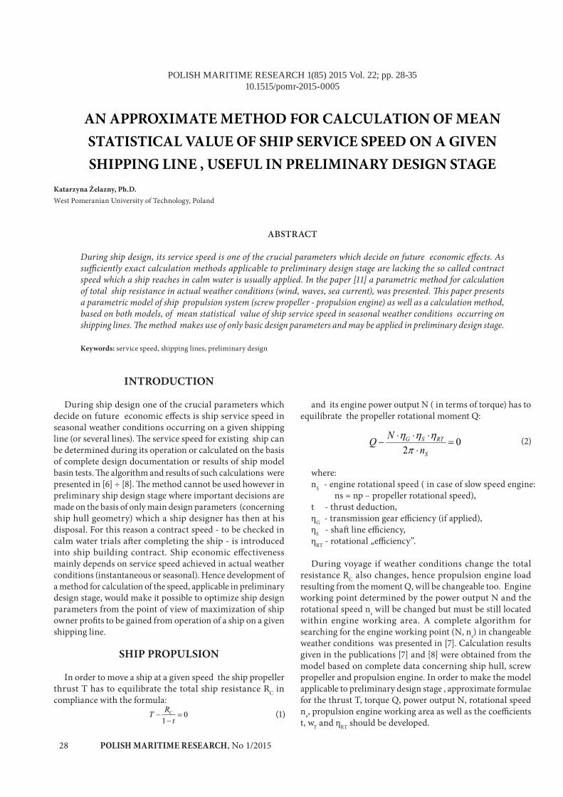
POLISH MARITIME RESEARCH, No 1/201528
POLISH MARITIME RESEARCH 1(85) 2015 Vol. 22; pp. 28-3510.1515/pomr-2015-0005
AN APPROXIMATE METHOD FOR CALCULATION OF MEAN STATISTICAL VALUE OF SHIP SERVICE SPEED ON A GIVEN SHIPPING LINE , USEFUL IN PRELIMINARY DESIGN STAGE
Katarzyna Żelazny, Ph.D.West Pomeranian University of Technology, Poland
ABSTRACT
During ship design, its service speed is one of the crucial parameters which decide on future economic effects. As sufficiently exact calculation methods applicable to preliminary design stage are lacking the so called contract speed which a ship reaches in calm water is usually applied. In the paper [11] a parametric method for calculation of total ship resistance in actual weather conditions (wind, waves, sea current), was presented. This paper presents a parametric model of ship propulsion system (screw propeller - propulsion engine) as well as a calculation method, based on both models, of mean statistical value of ship service speed in seasonal weather conditions occurring on shipping lines. The method makes use of only basic design parameters and may be applied in preliminary design stage.
Keywords: service speed, shipping lines, preliminary design
INTRODUCTION
During ship design one of the crucial parameters which decide on future economic effects is ship service speed in seasonal weather conditions occurring on a given shipping line (or several lines). The service speed for existing ship can be determined during its operation or calculated on the basis of complete design documentation or results of ship model basin tests. The algorithm and results of such calculations were presented in [6] ÷ [8]. The method cannot be used however in preliminary ship design stage where important decisions are made on the basis of only main design parameters (concerning ship hull geometry) which a ship designer has then at his disposal. For this reason a contract speed - to be checked in calm water trials after completing the ship - is introduced into ship building contract. Ship economic effectiveness mainly depends on service speed achieved in actual weather conditions (instantaneous or seasonal). Hence development of a method for calculation of the speed, applicable in preliminary design stage, would make it possible to optimize ship design parameters from the point of view of maximization of ship owner profits to be gained from operation of a ship on a given shipping line.
SHIP PROPULSION
In order to move a ship at a given speed the ship propeller thrust T has to equilibrate the total ship resistance RC in compliance with the formula:
(1)
and its engine power output N ( in terms of torque) has to equilibrate the propeller rotational moment Q:
(2)
where:nS - engine rotational speed ( in case of slow speed engine:
ns = np – propeller rotational speed), t - thrust deduction,ηG - transmission gear efficiency (if applied),ηS - shaft line efficiency,ηRT - rotational „efficiency”.
During voyage if weather conditions change the total resistance RC also changes, hence propulsion engine load resulting from the moment Q, will be changeable too. Engine working point determined by the power output N and the rotational speed ns will be changed but must be still located within engine working area. A complete algorithm for searching for the engine working point (N, ns) in changeable weather conditions was presented in [7]. Calculation results given in the publications [7] and [8] were obtained from the model based on complete data concerning ship hull, screw propeller and propulsion engine. In order to make the model applicable to preliminary design stage , approximate formulae for the thrust T, torque Q, power output N, rotational speed ns, propulsion engine working area as well as the coefficients t, wT and ηRT should be developed.
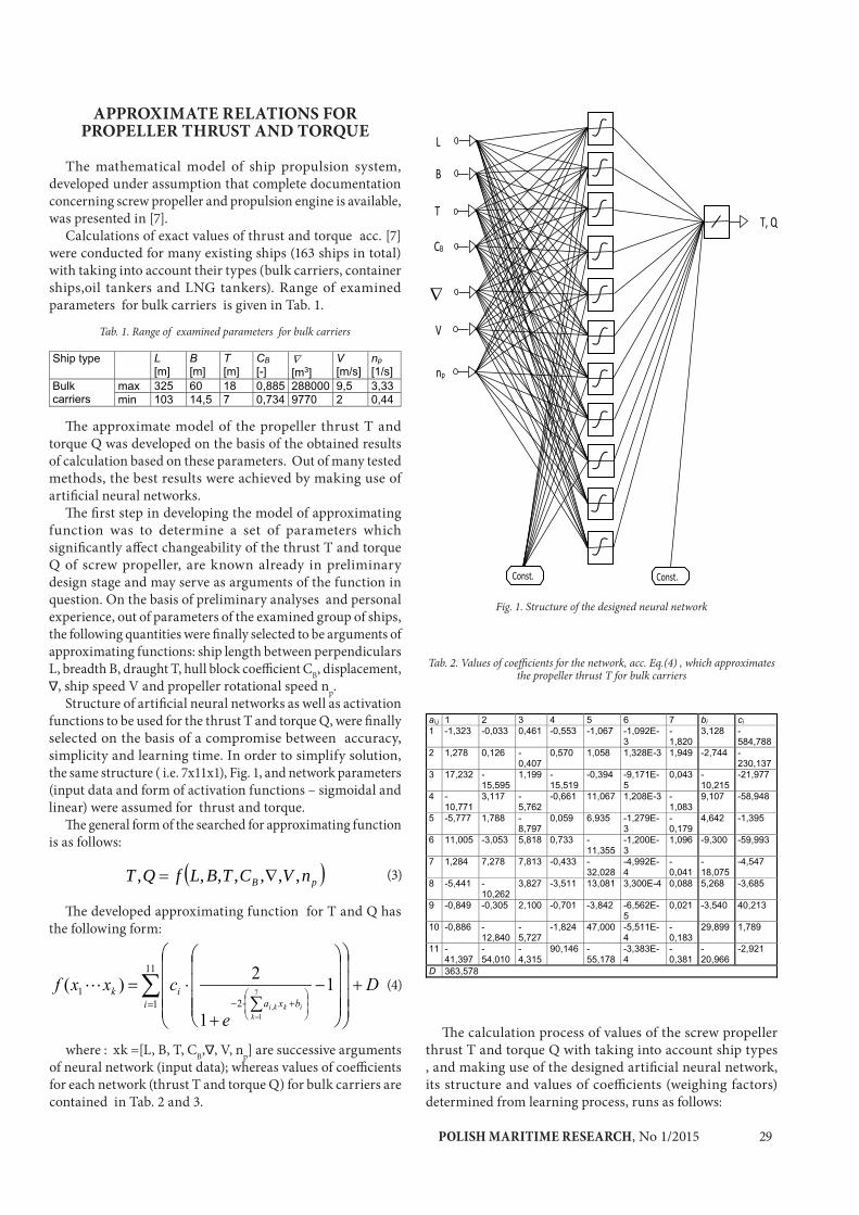
POLISH MARITIME RESEARCH, No 1/2015 29
APPROXIMATE RELATIONS FOR PROPELLER THRUST AND TORQUE
The mathematical model of ship propulsion system, developed under assumption that complete documentation concerning screw propeller and propulsion engine is available, was presented in [7].
Calculations of exact values of thrust and torque acc. [7] were conducted for many existing ships (163 ships in total) with taking into account their types (bulk carriers, container ships,oil tankers and LNG tankers). Range of examined parameters for bulk carriers is given in Tab. 1.
Tab. 1. Range of examined parameters for bulk carriers
The approximate model of the propeller thrust T and torque Q was developed on the basis of the obtained results of calculation based on these parameters. Out of many tested methods, the best results were achieved by making use of artificial neural networks.
The first step in developing the model of approximating function was to determine a set of parameters which significantly affect changeability of the thrust T and torque Q of screw propeller, are known already in preliminary design stage and may serve as arguments of the function in question. On the basis of preliminary analyses and personal experience, out of parameters of the examined group of ships, the following quantities were finally selected to be arguments of approximating functions: ship length between perpendiculars L, breadth B, draught T, hull block coefficient CB, displacement,
, ship speed V and propeller rotational speed np.Structure of artificial neural networks as well as activation
functions to be used for the thrust T and torque Q, were finally selected on the basis of a compromise between accuracy, simplicity and learning time. In order to simplify solution, the same structure ( i.e. 7x11x1), Fig. 1, and network parameters (input data and form of activation functions – sigmoidal and linear) were assumed for thrust and torque.
The general form of the searched for approximating function is as follows:
pB nVCTBLfQT ,,,,,,, (3)
The developed approximating function for T and Q has the following form:
(4)
where : xk =[L, B, T, CB, , V, np] are successive arguments of neural network (input data); whereas values of coefficients for each network (thrust T and torque Q) for bulk carriers are contained in Tab. 2 and 3.
Fig. 1. Structure of the designed neural network
Tab. 2. Values of coefficients for the network, acc. Eq.(4) , which approximates the propeller thrust T for bulk carriers
The calculation process of values of the screw propeller thrust T and torque Q with taking into account ship types , and making use of the designed artificial neural network, its structure and values of coefficients (weighing factors) determined from learning process, runs as follows:
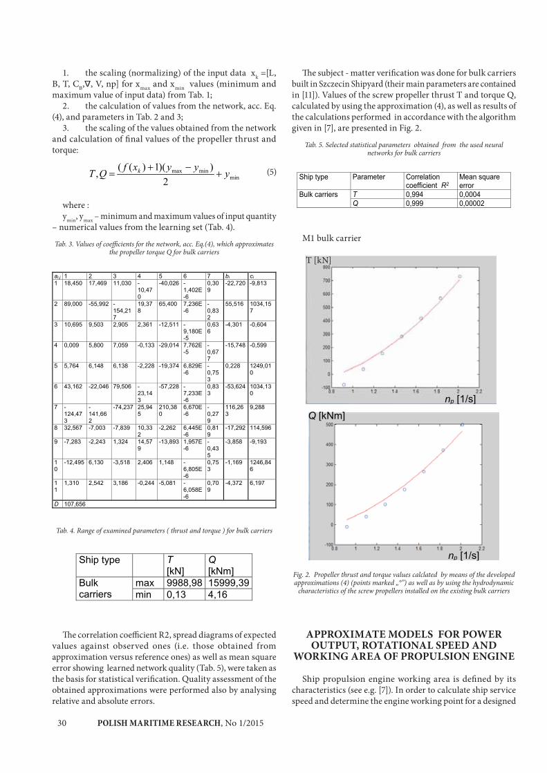
POLISH MARITIME RESEARCH, No 1/201530
1. the scaling (normalizing) of the input data xk =[L, B, T, CB, , V, np] for xmax and xmin values (minimum and maximum value of input data) from Tab. 1;
2. the calculation of values from the network, acc. Eq. (4), and parameters in Tab. 2 and 3;
3. the scaling of the values obtained from the network and calculation of final values of the propeller thrust and torque:
(5)
where : ymin, ymax – minimum and maximum values of input quantity
– numerical values from the learning set (Tab. 4).
Tab. 3. Values of coefficients for the network, acc. Eq.(4), which approximates the propeller torque Q for bulk carriers
Tab. 4. Range of examined parameters ( thrust and torque ) for bulk carriers
The correlation coefficient R2, spread diagrams of expected values against observed ones (i.e. those obtained from approximation versus reference ones) as well as mean square error showing learned network quality (Tab. 5), were taken as the basis for statistical verification. Quality assessment of the obtained approximations were performed also by analysing relative and absolute errors.
The subject - matter verification was done for bulk carriers built in Szczecin Shipyard (their main parameters are contained in [11]). Values of the screw propeller thrust T and torque Q, calculated by using the approximation (4), as well as results of the calculations performed in accordance with the algorithm given in [7], are presented in Fig. 2.
Tab. 5. Selected statistical parameters obtained from the used neural networks for bulk carriers
M1 bulk carrier
T [kN]
Fig. 2. Propeller thrust and torque values calclated by means of the developed approximations (4) (points marked „°”) as well as by using the hydrodynamic
characteristics of the screw propellers installed on the existing bulk carriers
APPROXIMATE MODELS FOR POWER OUTPUT, ROTATIONAL SPEED AND
WORKING AREA OF PROPULSION ENGINE
Ship propulsion engine working area is defined by its characteristics (see e.g. [7]). In order to calculate ship service speed and determine the engine working point for a designed
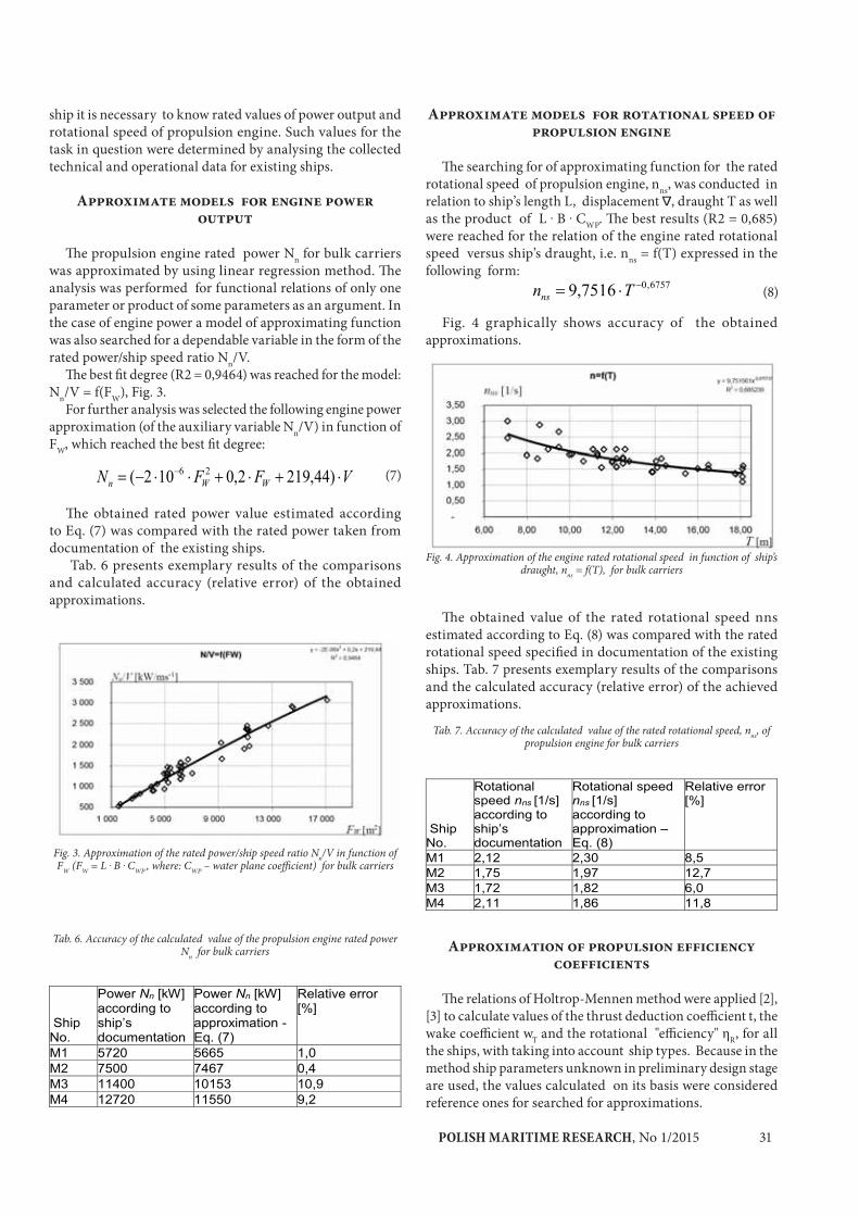
POLISH MARITIME RESEARCH, No 1/2015 31
ship it is necessary to know rated values of power output and rotational speed of propulsion engine. Such values for the task in question were determined by analysing the collected technical and operational data for existing ships.
Approximate models for engine power output
The propulsion engine rated power Nn for bulk carriers was approximated by using linear regression method. The analysis was performed for functional relations of only one parameter or product of some parameters as an argument. In the case of engine power a model of approximating function was also searched for a dependable variable in the form of the rated power/ship speed ratio Nn/V.
The best fit degree (R2 = 0,9464) was reached for the model: Nn/V = f(FW), Fig. 3.
For further analysis was selected the following engine power approximation (of the auxiliary variable Nn/V) in function of FW, which reached the best fit degree:
(7)
The obtained rated power value estimated according to Eq. (7) was compared with the rated power taken from documentation of the existing ships.
Tab. 6 presents exemplary results of the comparisons and calculated accuracy (relative error) of the obtained approximations.
Fig. 3. Approximation of the rated power/ship speed ratio Nn/V in function of FW (FW = L . B . CWP , where: CWP – water plane coefficient) for bulk carriers
Tab. 6. Accuracy of the calculated value of the propulsion engine rated power Nn for bulk carriers
Approximate models for rotational speed of propulsion engine
The searching for of approximating function for the rated rotational speed of propulsion engine, nns, was conducted in relation to ship’s length L, displacement , draught T as well as the product of L . B . CWP. The best results (R2 = 0,685) were reached for the relation of the engine rated rotational speed versus ship’s draught, i.e. nns = f(T) expressed in the following form:
(8)
Fig. 4 graphically shows accuracy of the obtained approximations.
Fig. 4. Approximation of the engine rated rotational speed in function of ship’s draught, nns = f(T), for bulk carriers
The obtained value of the rated rotational speed nns estimated according to Eq. (8) was compared with the rated rotational speed specified in documentation of the existing ships. Tab. 7 presents exemplary results of the comparisons and the calculated accuracy (relative error) of the achieved approximations.
Tab. 7. Accuracy of the calculated value of the rated rotational speed, nns, of propulsion engine for bulk carriers
Approximation of propulsion efficiency coefficients
The relations of Holtrop-Mennen method were applied [2], [3] to calculate values of the thrust deduction coefficient t, the wake coefficient wT and the rotational "efficiency" ηR, for all the ships, with taking into account ship types. Because in the method ship parameters unknown in preliminary design stage are used, the values calculated on its basis were considered reference ones for searched for approximations.
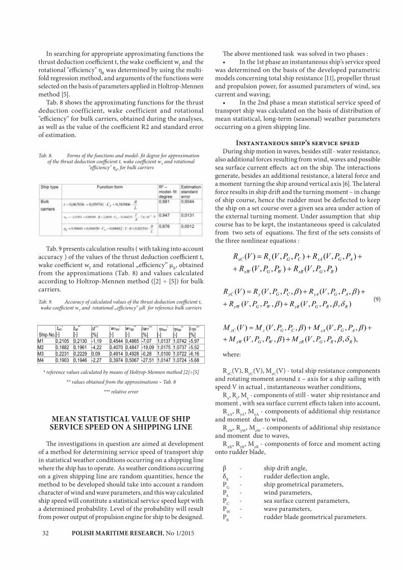
POLISH MARITIME RESEARCH, No 1/201532
In searching for appropriate approximating functions the thrust deduction coefficient t, the wake coefficient wT and the rotational "efficiency" ηR was determined by using the multi-fold regression method, and arguments of the functions were selected on the basis of parameters applied in Holtrop-Mennen method [5].
Tab. 8 shows the approximating functions for the thrust deduction coefficient, wake coefficient and rotational "efficiency" for bulk carriers, obtained during the analyses, as well as the value of the coefficient R2 and standard error of estimation.
Tab. 8. Forms of the functions and model- fit degree for approximation of the thrust deduction coefficient t, wake coefficient wT and rotational
"efficiency" ηR, for bulk carriers
Tab. 9 presents calculation results ( with taking into account accuracy ) of the values of the thrust deduction coefficient t, wake coefficient wT and rotational „efficiency” μR, obtained from the approximations (Tab. 8) and values calculated according to Holtrop-Mennen method ([2] ÷ [5]) for bulk carriers.
Tab. 9. Accuracy of calculated values of the thrust deduction coefficient t, wake coefficient wT and rotational „efficiency” μR for reference bulk carriers
* reference values calculated by means of Holtrop-Mennen method [2]÷[5]
** values obtained from the approximations – Tab. 8
*** relative error
MEAN STATISTICAL VALUE OF SHIP SERVICE SPEED ON A SHIPPING LINE
The investigations in question are aimed at development of a method for determining service speed of transport ship in statistical weather conditions occurring on a shipping line where the ship has to operate. As weather conditions occurring on a given shipping line are random quantities, hence the method to be developed should take into account a random character of wind and wave parameters, and this way calculated ship speed will constitute a statistical service speed kept with a determined probability. Level of the probability will result from power output of propulsion engine for ship to be designed.
The above mentioned task was solved in two phases :• In the 1st phase an instantaneous ship’s service speed
was determined on the basis of the developed parametric models concerning total ship resistance [11], propeller thrust and propulsion power, for assumed parameters of wind, sea current and waving;
• In the 2nd phase a mean statistical service speed of transport ship was calculated on the basis of distribution of mean statistical, long-term (seasonal) weather parameters occurring on a given shipping line.
Instantaneous ship’s service speed During ship motion in waves, besides still - water resistance,
also additional forces resulting from wind, waves and possible sea surface current effects act on the ship. The interactions generate, besides an additional resistance, a lateral force and a moment turning the ship around vertical axis [6]. The lateral force results in ship drift and the turning moment – in change of ship course, hence the rudder must be deflected to keep the ship on a set course over a given sea area under action of the external turning moment. Under assumption that ship course has to be kept, the instantaneous speed is calculated from two sets of equations. The first of the sets consists of the three nonlinear equations :
(9)
where:
RxC(V), RyC(V), MzC(V) - total ship resistance components and rotating moment around z – axis for a ship sailing with speed V in actual , instantaneous weather conditions,
Rx, Ry, Mz - components of still - water ship resistance and moment , with sea surface current effects taken into account,
RxA, RyA, MzA - components of additional ship resistance and moment due to wind,
RxW, RyW, MzW - components of additional ship resistance and moment due to waves,
RxR, RyR, MzR - components of force and moment acting onto rudder blade,
β - ship drift angle,δR - rudder deflection angle,PG - ship geometrical parameters,PA - wind parameters,PC - sea surface current parameters,PW - wave parameters,PR - rudder blade geometrical parameters.
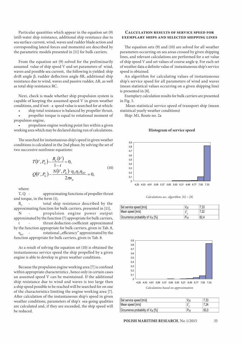
POLISH MARITIME RESEARCH, No 1/2015 33
Particular quantities which appear in the equation set (9) (still-water ship resistance, additional ship resistance due to sea surface current, wind, waves and rudder blade action and corresponding lateral forces and moments) are described by the parametric models presented in [11] for bulk carriers.
From the equation set (9) solved for the preliminarily assumed value of ship speed V and set parameters of wind, waves and possible sea current, the following is yielded: ship drift angle β, rudder deflection angle δR, additional ship resistance due to wind, waves and passive rudder, ΔR, as well as total ship resistance RC.
Next, check is made whether ship propulsion system is capable of keeping the assumed speed V in given weather conditions, and if not - a speed value is searched for at which:
• ship total resistance is balanced by propeller thrust, • propeller torque is equal to rotational moment of
propulsion engine, • propulsion engine working point lies within a given
working area which may be declared during run of calculations.
The searched for instantaneous ship’s speed in given weather conditions is calculated in the 2nd phase, by solving the set of two successive nonlinear equations:
(10)
where:T, Q - approximating functions of propeller thrust
and torque, in the form (1),RC - total ship resistance described by the
approximating function for bulk carriers, presented in [11],N - propulsion engine power output
approximated by the function (7) appropriate for bulk carriers,t - thrust deduction coefficient approximated
by the function appropriate for bulk carriers, given in Tab. 8,ηRT - rotational „efficiency” approximated by the
function appropriate for bulk carriers, given in Tab. 8.
As a result of solving the equation set (10) is obtained the instantaneous service speed the ship propelled by a given engine is able to develop in given weather conditions.
Because the propulsion engine working area [7] is confined within appropriate characteristics , hence only in certain cases an assumed speed V can be maintained. If the additional ship resistance due to wind and waves is too large then a ship speed possible to be reached will be searched for on one of the characteristics limiting the engine working area [7]. After calculation of the instantaneous ship’s speed in given weather conditions, parameters of ship’s sea-going qualities are calculated and, if they are exceeded, the ship speed will be reduced.
Calculation results of service speed for exemplary ships and selected shipping lines
The equation sets (9) and (10) are solved for all weather parameters occurring on sea areas crossed by given shipping lines, and relevant calculations are performed for a set value of ship speed V and set values of course angle ψ. For each set of weather data a definite value of instantaneous ship’s service speed is obtained.
An algorithm for calculating values of instantaneous ship’s service speed for all parameters of wind and waves (mean statistical values occurring on a given shipping line) is presented in [8].
Exemplary calculation results for bulk carriers are presented in Fig. 5.
Mean statistical service speed of transport ship (mean statistical yearly weather conditions)
Ship: M1, Route no. 2a
Histogram of service speed
Calculations acc. algorithm: [6] ÷ [8]
Calculations based on approximation
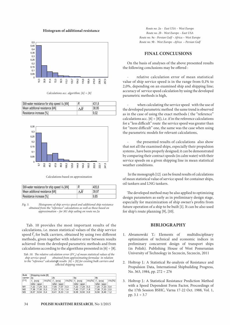
POLISH MARITIME RESEARCH, No 1/201534
Histogram of additional resistance
Calculations acc. algorithm: [6] ÷ [8]
Calculations based on approximation
Fig. 5. Histograms of ship service speed and additional ship resistance obtained from the “reference” calculations as well as those based on
approximation – for M1 ship sailing on route no.2a
Tab. 10 provides the most important results of the calculations, i.e. mean statistical values of the ship service speed for bulk carriers, obtained by using two different methods, given together with relative error between results achieved from the developed parametric methods and from calculations according to the algorithms presented in [6] ÷ [8].
Tab. 10. The relative calculation error (δVE) of mean statistical values of the ship service speed obtained from approximating formulae in relation
to the “reference” calculation results [6] ÷ [8] for existing bulk carriers and selected shipping routes
Route no. 2a - East USA – West Europe Route no. 2b - West Europe – East USA
Route no. 9a - Persian Gulf – Africa – West Europe Route no. 9b - West Europe –Africa – Persian Gulf
FINAL CONCLUSIONS
On the basis of analyses of the above presented results the following conclusions may be offered :
- relative calculation error of mean statistical value of ship service speed is in the range from 0,1% to 2,0%, depending on an examined ship and shipping line; accuracy of service speed calculation by using the developed parametric methods is high,
- when calculating the service speed with the use of the developed parametric method the same trend is observed as in the case of using the exact methods ( the “reference” calculations acc. [6] ÷ [8]), i.e. if in the reference calculations for a “less difficult” route the service speed was greater than for “more difficult” one, the same was the case when using the parametric models for relevant calculations,
- the presented results of calculations also show that not all the examined ships, especially their propulsion systems , have been properly designed; it can be demonstrated by comparing their contract speeds (in calm water) with their service speeds on a given shipping line in mean statistical weather conditions.
In the monograph [12] can be found results of calculations
of mean statistical value of service speed for container ships, oil tankers and LNG tankers.
The developed method may be also applied to optimizing design parameters as early as in preliminary design stage, especially for maximization of ship owner’s profits from future operation of a ship to be built [1]. It can be also used for ship’s route planning [9], [10].
BIBLIOGRAPHY
1. Abramowski T.: Elements of multidisciplinary optimization of technical and economic indices in preliminary concurrent design of transport ships (in Polish). Publishing House of West Pomeranian University of Technology in Szczecin, Szczecin, 2011
2. Holtrop J.: A Statistical Re-analysis of Resistance and Propulsion Data, International Shipbuilding Progress, No. 363, 1984, pp. 272 ÷ 276
3. Holtrop J.: A Statistical Resistance Prediction Method with a Speed Dependent Form Factor, Proceedings of the 17th Session BSHC, Varna 17-22 Oct. 1988, Vol. 1, pp. 3.1 ÷ 3.7

POLISH MARITIME RESEARCH, No 1/2015 35
4. Holtrop J.: A statistical analysis of performance test result, International Shipbuilding Progress, Vol. 24, No. 270, 1977, pp. 23 ÷ 28
5. Holtrop J., Mennen G. G. J.: An Approximate Power Prediction Method, International Shipbuilding Progress, Vol. 29, No. 335, 1982, pp. 166 ÷ 170
6. Szelangiewicz T., Żelazny K.: Calculation of the Mean Long-Term Service Speed of Transport Ship, Part I: Resistance of Ship Sailing on Regular Shipping Route in Real Weather Conditions, Polish Maritime Research, No. 4(50), Vol. 13, 2006, pp. 23 ÷ 31,
7. Szelangiewicz T., Żelazny K.: Calculation of Mean Long-Term Service Speed of Transport Ship, Part II: Service Speed of Ship Sailing on Regular Shipping Route in Real Weather Conditions, Polish Maritime Research, No 1,Vol. 14, 2007, pp. 28 ÷ 32,
8. Szelangiewicz T., Żelazny K.: Calculation of Mean Long-Term Service Speed of Transport Ship, Part III: Influence of Shipping Route and Ship Parameters on its Service Speed, Polish Maritime Research, No 2, Vol. 14, 2007, pp. 27 ÷ 32
9. Szelangiewicz T., Wiśniewski B., Żelazny K.: Forecasting operating speed of the ship in the selected weather conditions, EXPLO-SHIP 2014, Zeszyty Naukowe ( Scientific bulletins) No. 38(110),Szczecin Maritime University, Szczecin 2014, pp. 89 ÷ 98
10. Szelangiewicz T., Wiśniewski B., Żelazny K.: The influence of wind, wave and loading condition on total resistance and speed of the vessel, Polish Maritime Research, No 3(83), Vol. 21, 2014, pp. 61 ÷ 67
11. Żelazny K.: A method for determination of service speed of transport ships in statistical weather conditions occurring on shipping lines , useful in preliminary design stage ( in Polish ). A monograph ( to be published in 2015 by Publishing House of West Pomeranian University of Technology in Szczecin )
CONTACT WITH THE AUTHOR
Katarzyna Żelazny
West Pomeranian University of Technology Faculty of Maritime Technology and Transport
41 Piastów Ave. 71-065 Szczecin
POLAND

POLISH MARITIME RESEARCH, No 1/201536
POLISH MARITIME RESEARCH 1(85) 2015 Vol. 22; pp. 36-4610.1515/pomr-2015-0006
DESIGN AND STRENGTH CALCULATIONS OF THE TRIPOD SUPPORT STRUCTURE FOR OFFSHORE POWER PLANT
C. Dymarski, Prof.P. Dymarski, Ph. D.J. Żywicki, Ms. C.Gdańsk University of Technology, Poland
ABSTRACT
The support structure being the object of the analysis presented in the article is Tripod. According to the adopted assumptions, it is a foundation gravitationally set in the water region of 60 m in depth, not fixed to the seabed, which can be used for installing a 7MW wind turbine. Due to the lack of substantial information on designing and strength calculations of such types of structures in the world literature, authors have made an attempt to solve this problem within the framework of the abovementioned project. In the performed calculations all basic loads acting on the structure were taken into account, including: the self mass of the structure, the masses of the ballast, the tower and the turbine, as well as hydrostatic forces, and aero- and hydrodynamic forces acting on the entire object in extreme operating conditions.
Keywords: offshore wind turbine, support structure, Morison equation, FEM
INTRODUCTION
The here presented work has been done within the framework of the research project AQUILO entitled “Development of methods for the selection of the type of support structure for offshore wind turbine in Polish sea areas”.
The purpose of the task in which this research was implemented was to design a support structure in a given area of the Polish economic zone on the Baltic Sea. Within this project four types of structures were analysed: a gravity base, a tripod with pile foundation, a gravity tripod, and a deep water monopile.
Fig. 1a. Three types of support structures analyzed within the framework of the project - Gravity base
Fig. 1b. Three types of support structures analyzed within the framework of the project - Gravity tripod
The support structure being the object of the analysis presented in the article is Tripod. According to the adopted assumptions, it is a gravitationally set foundation, not fixed to the seabed, which can be used for installing a 7MW wind turbine in the water region of 60 m in depth. Due to the lack
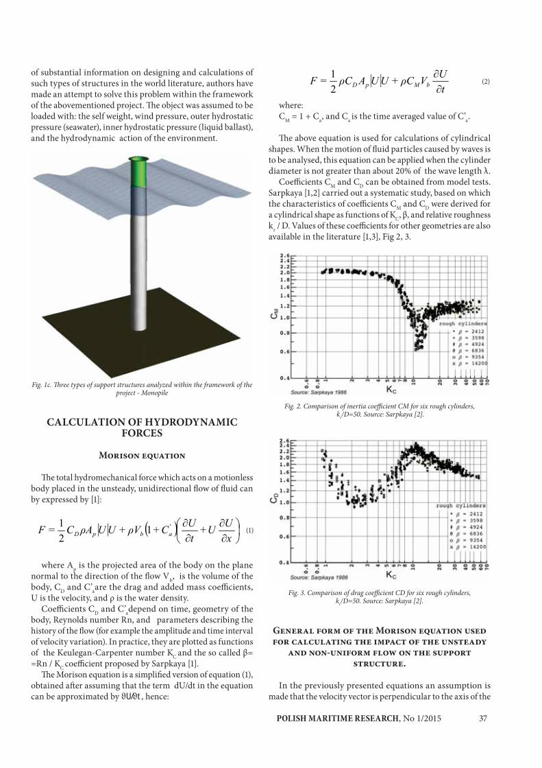
POLISH MARITIME RESEARCH, No 1/2015 37
of substantial information on designing and calculations of such types of structures in the world literature, authors have made an attempt to solve this problem within the framework of the abovementioned project. The object was assumed to be loaded with: the self weight, wind pressure, outer hydrostatic pressure (seawater), inner hydrostatic pressure (liquid ballast), and the hydrodynamic action of the environment.
Fig. 1c. Three types of support structures analyzed within the framework of the project - Monopile
CALCULATION OF HYDRODYNAMIC FORCES
Morison equation The total hydromechanical force which acts on a motionless
body placed in the unsteady, unidirectional flow of fluid can by expressed by [1]:
(1)
where Ap is the projected area of the body on the plane normal to the direction of the flow Vb, is the volume of the body, CD and C’aare the drag and added mass coefficients, U is the velocity, and ρ is the water density.
Coefficients CD and C’adepend on time, geometry of the body, Reynolds number Rn, and parameters describing the history of the flow (for example the amplitude and time interval of velocity variation). In practice, they are plotted as functions of the Keulegan-Carpenter number KC and the so called β= =Rn / KC coefficient proposed by Sarpkaya [1].
The Morison equation is a simplified version of equation (1), obtained after assuming that the term dU/dt in the equation can be approximated by ϑU/ϑt , hence:
(2)
where:CM = 1 + Ca, and Ca is the time averaged value of C’a.
The above equation is used for calculations of cylindrical shapes. When the motion of fluid particles caused by waves is to be analysed, this equation can be applied when the cylinder diameter is not greater than about 20% of the wave length λ.
Coefficients CM and CD can be obtained from model tests. Sarpkaya [1,2] carried out a systematic study, based on which the characteristics of coefficients CM and CD were derived for a cylindrical shape as functions of KC, β, and relative roughness kr / D. Values of these coefficients for other geometries are also available in the literature [1,3], Fig 2, 3.
Fig. 2. Comparison of inertia coefficient CM for six rough cylinders, kr/D=50. Source: Sarpkaya [2].
Fig. 3. Comparison of drag coefficient CD for six rough cylinders, kr/D=50. Source: Sarpkaya [2].
General form of the Morison equation used for calculating the impact of the unsteady
and non-uniform flow on the support structure.
In the previously presented equations an assumption is made that the velocity vector is perpendicular to the axis of the
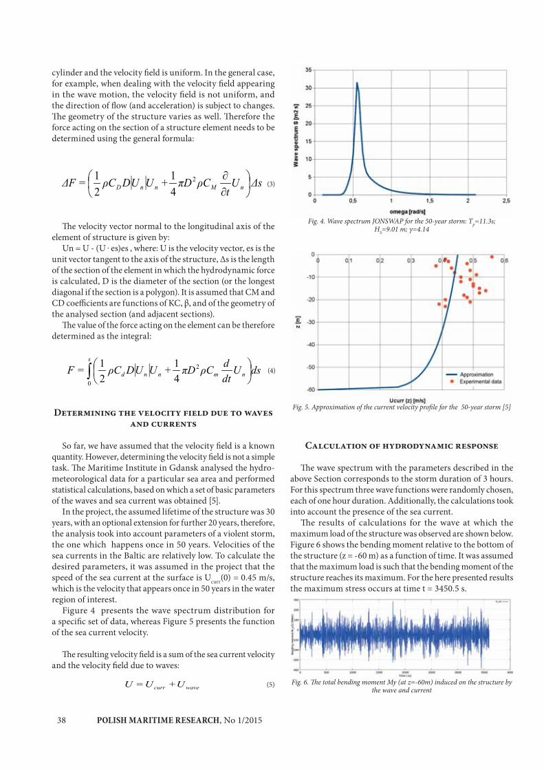
POLISH MARITIME RESEARCH, No 1/201538
cylinder and the velocity field is uniform. In the general case, for example, when dealing with the velocity field appearing in the wave motion, the velocity field is not uniform, and the direction of flow (and acceleration) is subject to changes. The geometry of the structure varies as well. Therefore the force acting on the section of a structure element needs to be determined using the general formula:
(3)
The velocity vector normal to the longitudinal axis of the element of structure is given by:
Un = U - (U . es)es , where: U is the velocity vector, es is the unit vector tangent to the axis of the structure, Δs is the length of the section of the element in which the hydrodynamic force is calculated, D is the diameter of the section (or the longest diagonal if the section is a polygon). It is assumed that CM and CD coefficients are functions of KC, β, and of the geometry of the analysed section (and adjacent sections).
The value of the force acting on the element can be therefore determined as the integral:
(4)
Determining the velocity field due to waves and currents
So far, we have assumed that the velocity field is a known quantity. However, determining the velocity field is not a simple task. The Maritime Institute in Gdansk analysed the hydro-meteorological data for a particular sea area and performed statistical calculations, based on which a set of basic parameters of the waves and sea current was obtained [5].
In the project, the assumed lifetime of the structure was 30 years, with an optional extension for further 20 years, therefore, the analysis took into account parameters of a violent storm, the one which happens once in 50 years. Velocities of the sea currents in the Baltic are relatively low. To calculate the desired parameters, it was assumed in the project that the speed of the sea current at the surface is Ucurr(0) = 0.45 m/s, which is the velocity that appears once in 50 years in the water region of interest.
Figure 4 presents the wave spectrum distribution for a specific set of data, whereas Figure 5 presents the function of the sea current velocity.
The resulting velocity field is a sum of the sea current velocity and the velocity field due to waves:
(5)
Fig. 4. Wave spectrum JONSWAP for the 50-year storm: Tp=11.3s; HS=9.01 m; γ=4.14
Fig. 5. Approximation of the current velocity profile for the 50-year storm [5]
Calculation of hydrodynamic response
The wave spectrum with the parameters described in the above Section corresponds to the storm duration of 3 hours. For this spectrum three wave functions were randomly chosen, each of one hour duration. Additionally, the calculations took into account the presence of the sea current.
The results of calculations for the wave at which the maximum load of the structure was observed are shown below. Figure 6 shows the bending moment relative to the bottom of the structure (z = -60 m) as a function of time. It was assumed that the maximum load is such that the bending moment of the structure reaches its maximum. For the here presented results the maximum stress occurs at time t = 3450.5 s.
Fig. 6. The total bending moment My (at z=-60m) induced on the structure by the wave and current

POLISH MARITIME RESEARCH, No 1/2015 39
DESCRIPTION OF THE INITIAL STRUCTURE
The foundation was designed as a thin-wall structure, the
shape of which resembles a tripod. Similar marine structures are already in operation, but they differ by foundation methods. For the time being, they have been used in more shallow waters and their legs were fixed to the seabed using piles. The here presented structure is intended to be used in conditions characteristic for the Baltic Sea, in its southern region at an approximate depth of 60 m, and is assumed to be founded on the seabed only with the aid of gravitational forces. That is why the shape of the lower part of the structure is designed in such a way that, after proper ballasting of the inside, the
foundation is ready to carry maximum loads taking place during its operation, with no shift with respect to the seabed. The support structure comprises a column divided into two basic parts. The upper part has the shape of a cone, with a ring on one end for mounting the wind turbine tower, while the lower part has the shape of a cylinder of 8 m in diameter. Three legs, evenly distributed by 120 degrees and inclined at 60 degrees to the vertical, are welded directly to the cylinder. The lower part of each of these legs is shaped as an elliptical cylinder with vertical walls, frequently referred to as the “hoof” or foot. The hoofs were connected together using horizontal pipes of about 1m in diameter. The footbase area is a circle of about 30 m in radius. The overall dimensions and thickness of the sheeting for preliminary calculations are given in Fig. 7.
Fig. 7. Basic geometric parameters of the support structure. [6]
(a) (b)
LOADS AND OPERATING CONDITIONS OF THE SUPPORT STRUCTURE
The below described loads and conditions of operation of the support structure are the same for each stage of structure geometry modifications described in the article. The presented results of consecutive simulations were obtained for these assumptions. As already mentioned, the structure was assumed to be founded in the Baltic Sea area at the depth of 60 m. The upper flange to which the column will be fixed is situated 15 m over the water surface. The loads of the structure coming from environmental conditions were generated during a hydromechanical simulation taking into account the conditions corresponding to the most violent storm in recent 50 years on the Baltic Sea. In these calculations, the worst conditions for the structure were assumed which take place when the wind loads, i.e. the thrust and the torque, mostly generated on the turbine, and the hydromechanical forces act along the same Y-direction.
Technical parameters of the turbine which were used for calculating foundation loads are collected in Tablel 1.
Based on the hydromechanical simulation, the distribution of horizontal loads coming from the sea current, waves, and the wind was determined as the function of the height of the object. For calculating purposes, the model was divided into 2-metre long segments, and the averaged horizontal load acting on each segment was calculated. The zero level was assumed at the bottom of the structure, while the water surface corresponded to the height of 60 m. The distribution of continuous load along the height of the structure is shown in Fig. 8. The forces coming from the aerodynamic drag of the tower, the thrust generated by the turbine, and the self weight were reduced to
Tab. 1: Technical parameters of the turbine
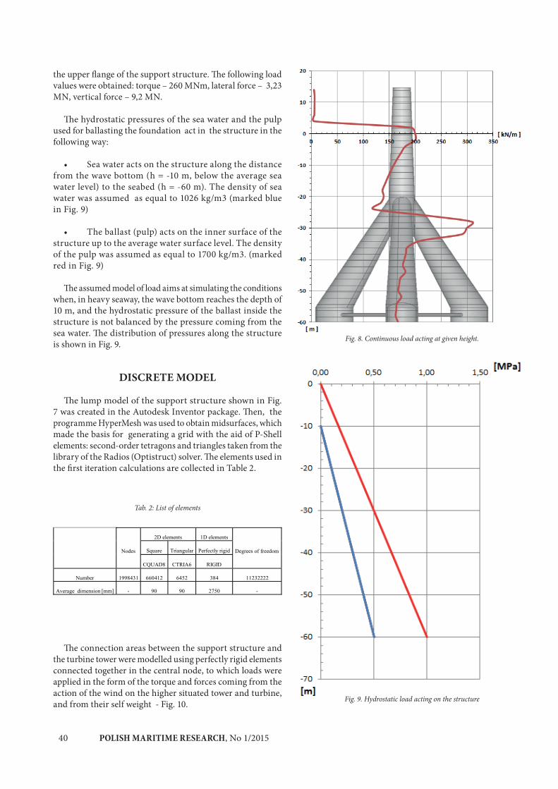
POLISH MARITIME RESEARCH, No 1/201540
the upper flange of the support structure. The following load values were obtained: torque – 260 MNm, lateral force – 3,23 MN, vertical force – 9,2 MN.
The hydrostatic pressures of the sea water and the pulp used for ballasting the foundation act in the structure in the following way:
• Sea water acts on the structure along the distance from the wave bottom (h = -10 m, below the average sea water level) to the seabed (h = -60 m). The density of sea water was assumed as equal to 1026 kg/m3 (marked blue in Fig. 9)
• The ballast (pulp) acts on the inner surface of the structure up to the average water surface level. The density of the pulp was assumed as equal to 1700 kg/m3. (marked red in Fig. 9)
The assumed model of load aims at simulating the conditions when, in heavy seaway, the wave bottom reaches the depth of 10 m, and the hydrostatic pressure of the ballast inside the structure is not balanced by the pressure coming from the sea water. The distribution of pressures along the structure is shown in Fig. 9. Fig. 8. Continuous load acting at given height.
Fig. 9. Hydrostatic load acting on the structure
DISCRETE MODEL
The lump model of the support structure shown in Fig. 7 was created in the Autodesk Inventor package. Then, the programme HyperMesh was used to obtain midsurfaces, which made the basis for generating a grid with the aid of P-Shell elements: second-order tetragons and triangles taken from the library of the Radios (Optistruct) solver. The elements used in the first iteration calculations are collected in Table 2.
The connection areas between the support structure and the turbine tower were modelled using perfectly rigid elements connected together in the central node, to which loads were applied in the form of the torque and forces coming from the action of the wind on the higher situated tower and turbine, and from their self weight - Fig. 10.
Tab. 2: List of elements

POLISH MARITIME RESEARCH, No 1/2015 41
Fig. 10. Central node „flange”
MODEL OF THE MATERIAL
The assumed linear-elastic model of the material revealed the following properties:
• Young’s modulus E = 210 GPa • Poisson ratio ν = 0.3 • density ρ = 7860 kg/m3
LOAD APPLICATION
According to the above description, the FEM model was loaded at the central point with a negative torque of about 260 MNm along the X-direction and the lateral force of 3.23 MN acting along the Y-direction.
The loads from the masses of the wind tower column (458 t), and the nacelle and rotor (480 t) were applied as the 9.2 MN force to the node on the upper flange.
The gravitational acceleration a = 9.81m/s2 with the negative sense was applied along the Z-direction. According to the assumptions described in the previous Section, the hydrodynamic load of the structure was applied to nodes along the Y-direction. The grid of the model was divided into horizontal segments of 2 m in height, and then the numbers of nodes composing particular segments were counted. Each of these nodes was loaded with a force which was calculated by dividing the total load of the given segment obtained from CFD simulation by the number of nodes. A decision to make use of the above model was dictated by the fact that hydrodynamic pressures are much smaller than hydrostatic pressures acting on the foundation. Their action generates the bending moment, which is a remarkable load for the structure. The adopted load distribution does not affect much the local strength of the structure, and remarkably facilitates data preparation for calculations. The hydrostatic pressure was applied along the normal direction to the seabed and the sheeting, according to the assumptions shown in Fig. 9.
FEM CALCULATIONS
The structure strength calculations were performed using the Finite Element Method (FEM) and the HyperWorks v12 package produced by Altair. The programme HyperMesh, which
in authors’ opinion is an excellent tool for grid preparation and imposing boundary conditions to such a large surface model, was used as preprocessor. Linear calculations were performed using the solver Optistruct, while the results were displayed using the postprocessor HyperView. The simulation was performed on PC equipped with a 4-core, 64-bit processor Intel I7 2.30 GHz, 16 GB of RAM DDR3, and the hard disc SSD 840 PRO. The calculations for the structure at final stages of geometry modifications, in which the number of finite surface elements was approximately equal to 1 million, took about 2.5 hours.
STRENGTH CALCULATIONS OF THE INITIAL STRUCTURE
For the purpose of preliminary analyses, a structure was worked out without inner stiffening elements in order to detect places which would require installation of additional structural elements. A motivation for this decision was to avoid excessive dimensioning of the structure. In the first simulation the model was fixed at the seabed by removing the ability to move in X,Y,Z-directions from the nodes composing the bottom of the structure.
Figures 11 and 12 show contour maps presenting the distributions of stresses [MPa] and deformations [mm] in the initial structure.
Fig. 11 Reduced stresses [MPa]
Fig. 12 Elastic deformations [mm]
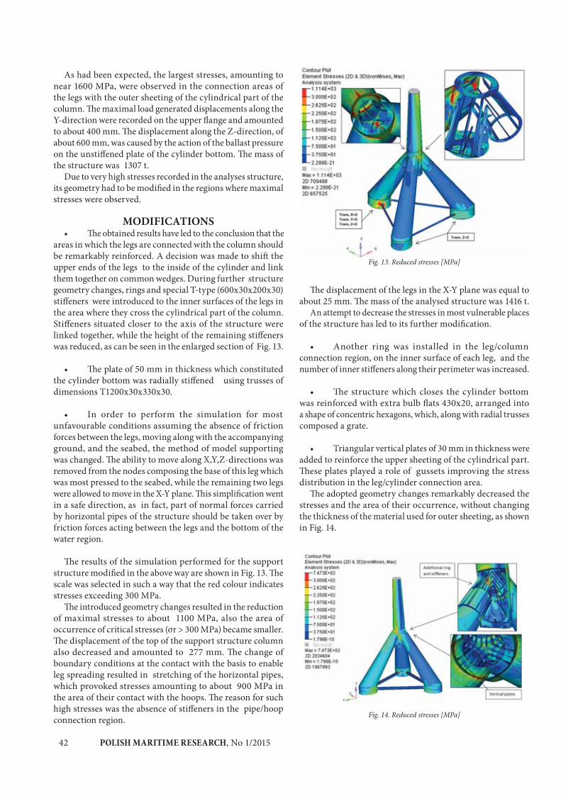
POLISH MARITIME RESEARCH, No 1/201542
As had been expected, the largest stresses, amounting to near 1600 MPa, were observed in the connection areas of the legs with the outer sheeting of the cylindrical part of the column. The maximal load generated displacements along the Y-direction were recorded on the upper flange and amounted to about 400 mm. The displacement along the Z-direction, of about 600 mm, was caused by the action of the ballast pressure on the unstiffened plate of the cylinder bottom. The mass of the structure was 1307 t.
Due to very high stresses recorded in the analyses structure, its geometry had to be modified in the regions where maximal stresses were observed.
MODIFICATIONS • The obtained results have led to the conclusion that the
areas in which the legs are connected with the column should be remarkably reinforced. A decision was made to shift the upper ends of the legs to the inside of the cylinder and link them together on common wedges. During further structure geometry changes, rings and special T-type (600x30x200x30) stiffeners were introduced to the inner surfaces of the legs in the area where they cross the cylindrical part of the column. Stiffeners situated closer to the axis of the structure were linked together, while the height of the remaining stiffeners was reduced, as can be seen in the enlarged section of Fig. 13.
• The plate of 50 mm in thickness which constituted the cylinder bottom was radially stiffened using trusses of dimensions T1200x30x330x30.
• In order to perform the simulation for most unfavourable conditions assuming the absence of friction forces between the legs, moving along with the accompanying ground, and the seabed, the method of model supporting was changed. The ability to move along X,Y,Z-directions was removed from the nodes composing the base of this leg which was most pressed to the seabed, while the remaining two legs were allowed to move in the X-Y plane. This simplification went in a safe direction, as in fact, part of normal forces carried by horizontal pipes of the structure should be taken over by friction forces acting between the legs and the bottom of the water region.
The results of the simulation performed for the support structure modified in the above way are shown in Fig. 13. The scale was selected in such a way that the red colour indicates stresses exceeding 300 MPa.
The introduced geometry changes resulted in the reduction of maximal stresses to about 1100 MPa, also the area of occurrence of critical stresses (σr > 300 MPa) became smaller. The displacement of the top of the support structure column also decreased and amounted to 277 mm. The change of boundary conditions at the contact with the basis to enable leg spreading resulted in stretching of the horizontal pipes, which provoked stresses amounting to about 900 MPa in the area of their contact with the hoops. The reason for such high stresses was the absence of stiffeners in the pipe/hoop connection region.
Fig. 13. Reduced stresses [MPa]
The displacement of the legs in the X-Y plane was equal to about 25 mm. The mass of the analysed structure was 1416 t.
An attempt to decrease the stresses in most vulnerable places of the structure has led to its further modification.
• Another ring was installed in the leg/column connection region, on the inner surface of each leg, and the number of inner stiffeners along their perimeter was increased.
• The structure which closes the cylinder bottom
was reinforced with extra bulb flats 430x20, arranged into a shape of concentric hexagons, which, along with radial trusses composed a grate.
• Triangular vertical plates of 30 mm in thickness were added to reinforce the upper sheeting of the cylindrical part. These plates played a role of gussets improving the stress distribution in the leg/cylinder connection area.
The adopted geometry changes remarkably decreased the stresses and the area of their occurrence, without changing the thickness of the material used for outer sheeting, as shown in Fig. 14.
Fig. 14. Reduced stresses [MPa]
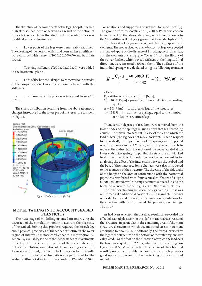
POLISH MARITIME RESEARCH, No 1/2015 43
The structure of the lower parts of the legs (hoops) in which high stresses had been observed as a result of the action of forces taken over from the stretched horizontal pipes was modified in the following way :
• Lower parts of the legs were remarkably modified. The sheeting of the bottom which had been earlier unstiffened was reinforced with trusses (T1000x30x300x30) and bulb flats 430x20.
• Two ring stiffeners (T500x30x200x30) were added in the horizontal plane.
• Ends of the horizontal pipes were moved to the insides of the hoops by about 1 m and additionally linked with the stiffeners.
• The diameter of the pipes was increased from z 1m to 2 m.
The stress distribution resulting from the above geometry changes introduced to the lower part of the structure is shown in Fig. 15.
Fig. 15. Reduced stresses [MPa]
MODEL TAKING INTO ACCOUNT SEABED PLASTICITY
The next stage of modelling oriented on improving the accuracy of the simulation took into account the plasticity of the seabed. Solving this problem required the knowledge about physical properties of the seabed structure in the water region of interest. It is noteworthy that this information is, generally, available, as one of the initial stages of investments projects of this type is examination of the seabed structure in the area of future foundation of the supporting structures. However at present, due to the lack of access to the results of this examination, the simulation was performed for the seabed stiffness taken from the standard PN-80/B-03040
“Foundations and supporting structures for machines” [7]. The ground stiffness coefficient Cz = 40 MPa/m was chosen from Table 1 in the above standard, which corresponds to the “low-stiffness II category ground, silty sands, hydrated”.
The plasticity of the ground was modelled using spring type elements. The nodes situated at the bottom of legs were copied and moved apart by the distance of 1 m along the Z-direction, and the elements of spring type “Celas_1” from the library of the solver Radios, which reveal stiffness at the longitudinal direction, were inserted between them. The stiffness of the individual spring was calculated using the following formula:
(6)
where:Ki – stiffness of a single spring [N/m];Cz = 40 [MPa/m] – ground stiffness coefficient, according
to [7];A = 308,9 [m2] – total area of legs of the structure; i = 134138 [-] – number of springs, equal to the number
of nodes on structure’s legs.
Then, certain degrees of freedom were removed from the lower nodes of the springs in such a way that leg spreading could still be taken into account. In case of the leg on which the load Y acts (the leg does not move horizontally with respect to the seabed), the upper nodes of the springs were deprived of ability to move in the XY plane, while they were still able to move in the Z-direction. The motion of the nodes situated at the lower ends of the springs supporting the structure was blocked in all three directions. This solution provided opportunities for analysing the effect of the interaction between the seabed and the base of the structure. Some changes were also introduced to the geometry of the structure. The sheeting of the side walls of the hoops in the area of connections with the horizontal pipes was reinforced with four vertical stiffeners of T type (300x30x200x30), while the pipe segments situated inside the hooks were reinforced with gussets of 30mm in thickness.
The cylinder sheeting between the legs coming into it was reinforced with additional horizontal ring segments. The way of model fixing and the results of simulation calculations for the structure with the introduced changes are shown in Figs. 16 and 17.
As had been expected, the obtained results have revealed the effect of seabed plasticity on the deformations and stresses of the structure, in particular in the contacting areas of the main structure elements in which the maximal stress increment amounted to about 6 %. Additionally, the forces exerted by the legs of the structure on the bottom of the water region were calculated. For the foot on the direction of which the load acts the force was equal to 1,02 MPa, while for the remaining two legs it was 0,68 MPa for each. The analysis of the obtained results proves their qualitative correctness, which provides good opportunities for further perfecting of the examined model.
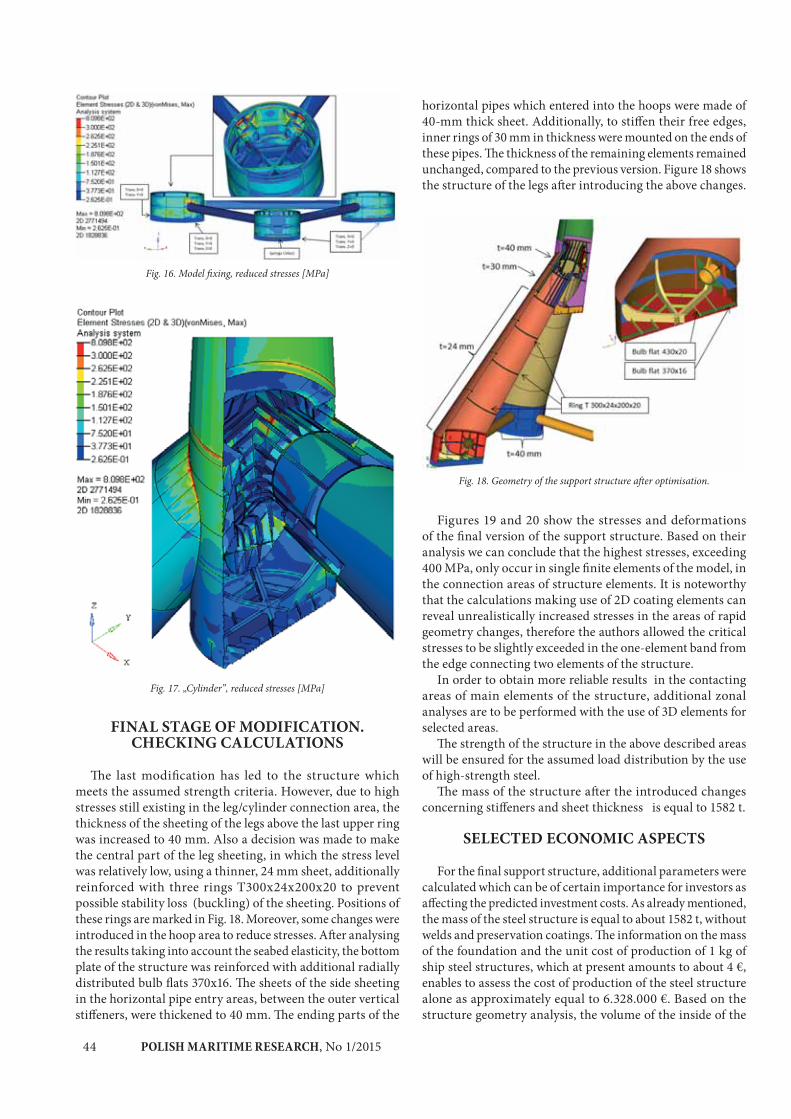
POLISH MARITIME RESEARCH, No 1/201544
Fig. 16. Model fixing, reduced stresses [MPa]
Fig. 17. „Cylinder”, reduced stresses [MPa]
FINAL STAGE OF MODIFICATION. CHECKING CALCULATIONS
The last modification has led to the structure which meets the assumed strength criteria. However, due to high stresses still existing in the leg/cylinder connection area, the thickness of the sheeting of the legs above the last upper ring was increased to 40 mm. Also a decision was made to make the central part of the leg sheeting, in which the stress level was relatively low, using a thinner, 24 mm sheet, additionally reinforced with three rings T300x24x200x20 to prevent possible stability loss (buckling) of the sheeting. Positions of these rings are marked in Fig. 18. Moreover, some changes were introduced in the hoop area to reduce stresses. After analysing the results taking into account the seabed elasticity, the bottom plate of the structure was reinforced with additional radially distributed bulb flats 370x16. The sheets of the side sheeting in the horizontal pipe entry areas, between the outer vertical stiffeners, were thickened to 40 mm. The ending parts of the
horizontal pipes which entered into the hoops were made of 40-mm thick sheet. Additionally, to stiffen their free edges, inner rings of 30 mm in thickness were mounted on the ends of these pipes. The thickness of the remaining elements remained unchanged, compared to the previous version. Figure 18 shows the structure of the legs after introducing the above changes.
Fig. 18. Geometry of the support structure after optimisation.
Figures 19 and 20 show the stresses and deformations of the final version of the support structure. Based on their analysis we can conclude that the highest stresses, exceeding 400 MPa, only occur in single finite elements of the model, in the connection areas of structure elements. It is noteworthy that the calculations making use of 2D coating elements can reveal unrealistically increased stresses in the areas of rapid geometry changes, therefore the authors allowed the critical stresses to be slightly exceeded in the one-element band from the edge connecting two elements of the structure.
In order to obtain more reliable results in the contacting areas of main elements of the structure, additional zonal analyses are to be performed with the use of 3D elements for selected areas.
The strength of the structure in the above described areas will be ensured for the assumed load distribution by the use of high-strength steel.
The mass of the structure after the introduced changes concerning stiffeners and sheet thickness is equal to 1582 t.
SELECTED ECONOMIC ASPECTS
For the final support structure, additional parameters were calculated which can be of certain importance for investors as affecting the predicted investment costs. As already mentioned, the mass of the steel structure is equal to about 1582 t, without welds and preservation coatings. The information on the mass of the foundation and the unit cost of production of 1 kg of ship steel structures, which at present amounts to about 4 €, enables to assess the cost of production of the steel structure alone as approximately equal to 6.328.000 €. Based on the structure geometry analysis, the volume of the inside of the
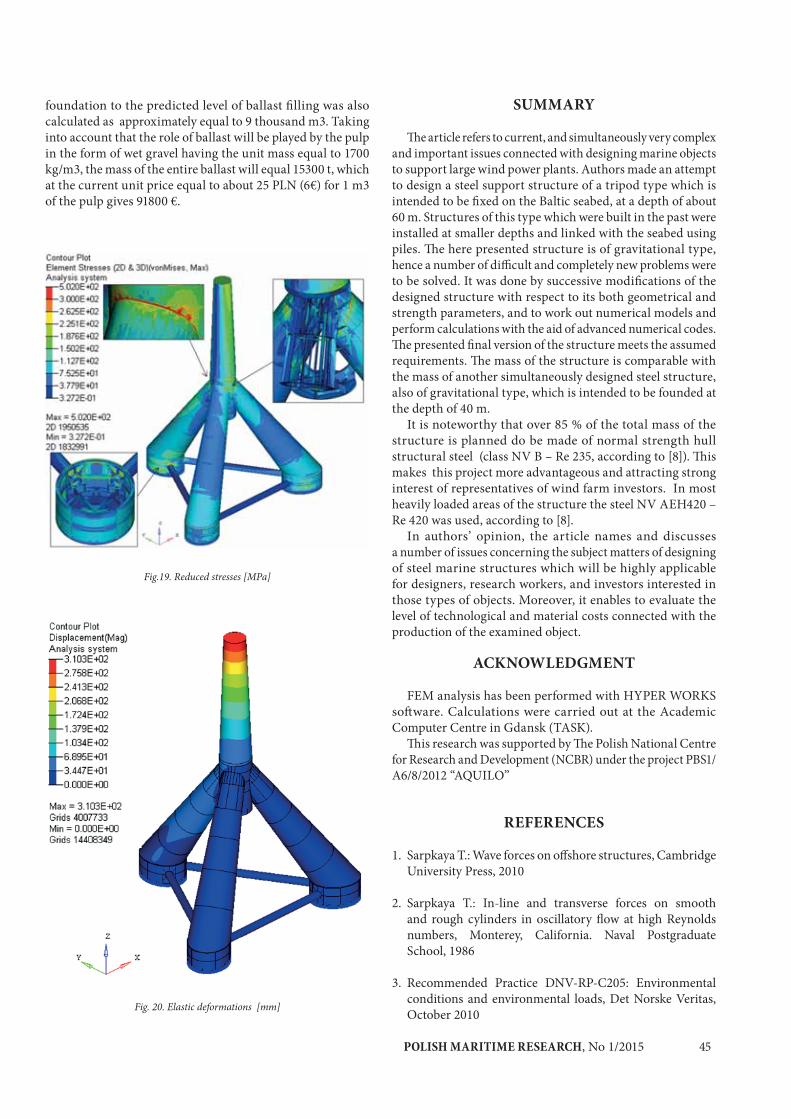
POLISH MARITIME RESEARCH, No 1/2015 45
foundation to the predicted level of ballast filling was also calculated as approximately equal to 9 thousand m3. Taking into account that the role of ballast will be played by the pulp in the form of wet gravel having the unit mass equal to 1700 kg/m3, the mass of the entire ballast will equal 15300 t, which at the current unit price equal to about 25 PLN (6€) for 1 m3 of the pulp gives 91800 €.
Fig.19. Reduced stresses [MPa]
Fig. 20. Elastic deformations [mm]
SUMMARY
The article refers to current, and simultaneously very complex and important issues connected with designing marine objects to support large wind power plants. Authors made an attempt to design a steel support structure of a tripod type which is intended to be fixed on the Baltic seabed, at a depth of about 60 m. Structures of this type which were built in the past were installed at smaller depths and linked with the seabed using piles. The here presented structure is of gravitational type, hence a number of difficult and completely new problems were to be solved. It was done by successive modifications of the designed structure with respect to its both geometrical and strength parameters, and to work out numerical models and perform calculations with the aid of advanced numerical codes. The presented final version of the structure meets the assumed requirements. The mass of the structure is comparable with the mass of another simultaneously designed steel structure, also of gravitational type, which is intended to be founded at the depth of 40 m.
It is noteworthy that over 85 % of the total mass of the structure is planned do be made of normal strength hull structural steel (class NV B – Re 235, according to [8]). This makes this project more advantageous and attracting strong interest of representatives of wind farm investors. In most heavily loaded areas of the structure the steel NV AEH420 – Re 420 was used, according to [8].
In authors’ opinion, the article names and discusses a number of issues concerning the subject matters of designing of steel marine structures which will be highly applicable for designers, research workers, and investors interested in those types of objects. Moreover, it enables to evaluate the level of technological and material costs connected with the production of the examined object.
ACKNOWLEDGMENT
FEM analysis has been performed with HYPER WORKS software. Calculations were carried out at the Academic Computer Centre in Gdansk (TASK).
This research was supported by The Polish National Centre for Research and Development (NCBR) under the project PBS1/A6/8/2012 “AQUILO”
REFERENCES
1. Sarpkaya T.: Wave forces on offshore structures, Cambridge University Press, 2010
2. Sarpkaya T.: In-line and transverse forces on smooth and rough cylinders in oscillatory flow at high Reynolds numbers, Monterey, California. Naval Postgraduate School, 1986
3. Recommended Practice DNV-RP-C205: Environmental conditions and environmental loads, Det Norske Veritas, October 2010

POLISH MARITIME RESEARCH, No 1/201546
4. Levis E.V.: Principles of Naval Architecture. Vol. III – Motions in Waves and Controllability, SNAME, 1989
5. Dymarski P., Ciba E., Marcinkowski T.: Effective method for determining environmental loads on supporting structures for offshore wind turbines, 20th International Conference on Hydrodynamics in Ship Design and Operation HYDRONAV 2014, Wroclaw, Poland, June 2014
6. Turbine graphics, source: Repower (in Polish)
7. PN-80/B-03040 „Foundations and supporting structures for machines” (in Polish)
8. DNV-OS-J101 Design of Offshore Wind Turbine Structures
CONTACT WITH THE AUTOR
Czesław Dymarski,Paweł Dymarski,Jędrzej Żywicki
Gdańsk University of Technology Faculty of Ocean Engineering and Ship Technology
11/12 Narutowicza Str. 80-233 Gdańsk
POLAND
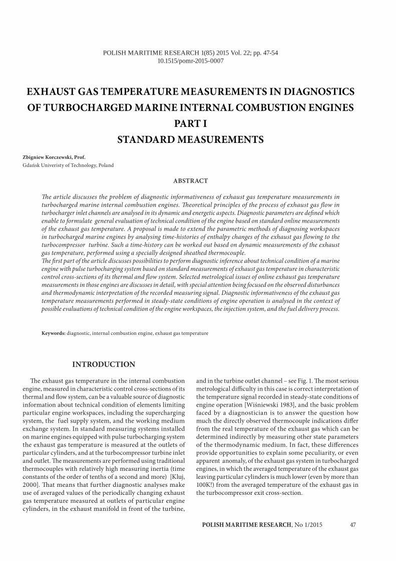
POLISH MARITIME RESEARCH, No 1/2015 47
POLISH MARITIME RESEARCH 1(85) 2015 Vol. 22; pp. 47-5410.1515/pomr-2015-0007
EXHAUST GAS TEMPERATURE MEASUREMENTS IN DIAGNOSTICS OF TURBOCHARGED MARINE INTERNAL COMBUSTION ENGINES
PART I STANDARD MEASUREMENTS
Zbigniew Korczewski, Prof.Gdańsk Univeristy of Technology, Poland
ABSTRACT
The article discusses the problem of diagnostic informativeness of exhaust gas temperature measurements in turbocharged marine internal combustion engines. Theoretical principles of the process of exhaust gas flow in turbocharger inlet channels are analysed in its dynamic and energetic aspects. Diagnostic parameters are defined which enable to formulate general evaluation of technical condition of the engine based on standard online measurements of the exhaust gas temperature. A proposal is made to extend the parametric methods of diagnosing workspaces in turbocharged marine engines by analysing time-histories of enthalpy changes of the exhaust gas flowing to the turbocompressor turbine. Such a time-history can be worked out based on dynamic measurements of the exhaust gas temperature, performed using a specially designed sheathed thermocouple.The first part of the article discusses possibilities to perform diagnostic inference about technical condition of a marine engine with pulse turbocharging system based on standard measurements of exhaust gas temperature in characteristic control cross-sections of its thermal and flow system. Selected metrological issues of online exhaust gas temperature measurements in those engines are discusses in detail, with special attention being focused on the observed disturbances and thermodynamic interpretation of the recorded measuring signal. Diagnostic informativeness of the exhaust gas temperature measurements performed in steady-state conditions of engine operation is analysed in the context of possible evaluations of technical condition of the engine workspaces, the injection system, and the fuel delivery process.
Keywords: diagnostic, internal combustion engine, exhaust gas temperature
INTRODUCTION
The exhaust gas temperature in the internal combustion engine, measured in characteristic control cross-sections of its thermal and flow system, can be a valuable source of diagnostic information about technical condition of elements limiting particular engine workspaces, including the supercharging system, the fuel supply system, and the working medium exchange system. In standard measuring systems installed on marine engines equipped with pulse turbocharging system the exhaust gas temperature is measured at the outlets of particular cylinders, and at the turbocompressor turbine inlet and outlet. The measurements are performed using traditional thermocouples with relatively high measuring inertia (time constants of the order of tenths of a second and more) [Kluj, 2000]. That means that further diagnostic analyses make use of averaged values of the periodically changing exhaust gas temperature measured at outlets of particular engine cylinders, in the exhaust manifold in front of the turbine,
and in the turbine outlet channel – see Fig. 1. The most serious metrological difficulty in this case is correct interpretation of the temperature signal recorded in steady-state conditions of engine operation [Wiśniewski 1983], and the basic problem faced by a diagnostician is to answer the question how much the directly observed thermocouple indications differ from the real temperature of the exhaust gas which can be determined indirectly by measuring other state parameters of the thermodynamic medium. In fact, these differences provide opportunities to explain some peculiarity, or even apparent anomaly, of the exhaust gas system in turbocharged engines, in which the averaged temperature of the exhaust gas leaving particular cylinders is much lower (even by more than 100K!) from the averaged temperature of the exhaust gas in the turbocompressor exit cross-section.
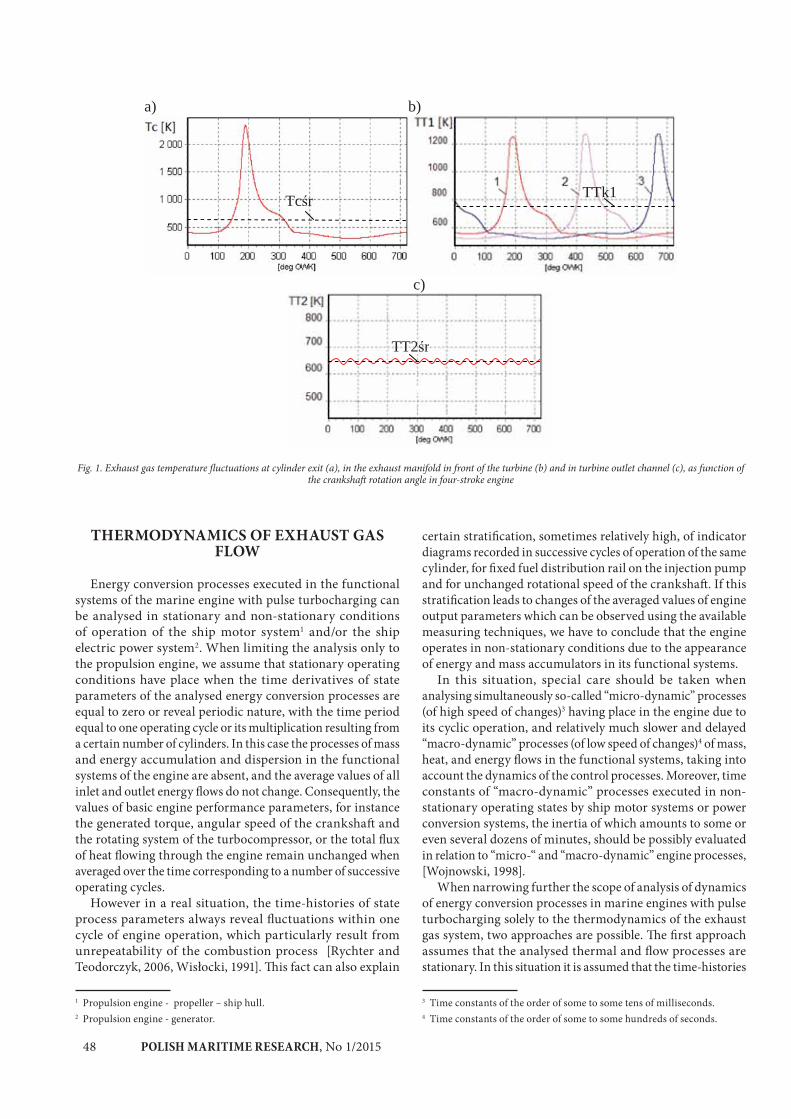
POLISH MARITIME RESEARCH, No 1/201548
THERMODYNAMICS OF EXHAUST GAS FLOW
Energy conversion processes executed in the functional systems of the marine engine with pulse turbocharging can be analysed in stationary and non-stationary conditions of operation of the ship motor system1 and/or the ship electric power system2. When limiting the analysis only to the propulsion engine, we assume that stationary operating conditions have place when the time derivatives of state parameters of the analysed energy conversion processes are equal to zero or reveal periodic nature, with the time period equal to one operating cycle or its multiplication resulting from a certain number of cylinders. In this case the processes of mass and energy accumulation and dispersion in the functional systems of the engine are absent, and the average values of all inlet and outlet energy flows do not change. Consequently, the values of basic engine performance parameters, for instance the generated torque, angular speed of the crankshaft and the rotating system of the turbocompressor, or the total flux of heat flowing through the engine remain unchanged when averaged over the time corresponding to a number of successive operating cycles.
However in a real situation, the time-histories of state process parameters always reveal fluctuations within one cycle of engine operation, which particularly result from unrepeatability of the combustion process [Rychter and Teodorczyk, 2006, Wisłocki, 1991]. This fact can also explain
1 Propulsion engine - propeller – ship hull.2 Propulsion engine - generator.
certain stratification, sometimes relatively high, of indicator diagrams recorded in successive cycles of operation of the same cylinder, for fixed fuel distribution rail on the injection pump and for unchanged rotational speed of the crankshaft. If this stratification leads to changes of the averaged values of engine output parameters which can be observed using the available measuring techniques, we have to conclude that the engine operates in non-stationary conditions due to the appearance of energy and mass accumulators in its functional systems.
In this situation, special care should be taken when analysing simultaneously so-called “micro-dynamic” processes (of high speed of changes)3 having place in the engine due to its cyclic operation, and relatively much slower and delayed “macro-dynamic” processes (of low speed of changes)4 of mass, heat, and energy flows in the functional systems, taking into account the dynamics of the control processes. Moreover, time constants of “macro-dynamic” processes executed in non-stationary operating states by ship motor systems or power conversion systems, the inertia of which amounts to some or even several dozens of minutes, should be possibly evaluated in relation to “micro-“ and “macro-dynamic” engine processes, [Wojnowski, 1998].
When narrowing further the scope of analysis of dynamics of energy conversion processes in marine engines with pulse turbocharging solely to the thermodynamics of the exhaust gas system, two approaches are possible. The first approach assumes that the analysed thermal and flow processes are stationary. In this situation it is assumed that the time-histories
3 Time constants of the order of some to some tens of milliseconds.4 Time constants of the order of some to some hundreds of seconds.
a) b)
c)
Tc r
TT2 r
TTk1
Fig. 1. Exhaust gas temperature fluctuations at cylinder exit (a), in the exhaust manifold in front of the turbine (b) and in turbine outlet channel (c), as function of the crankshaft rotation angle in four-stroke engine
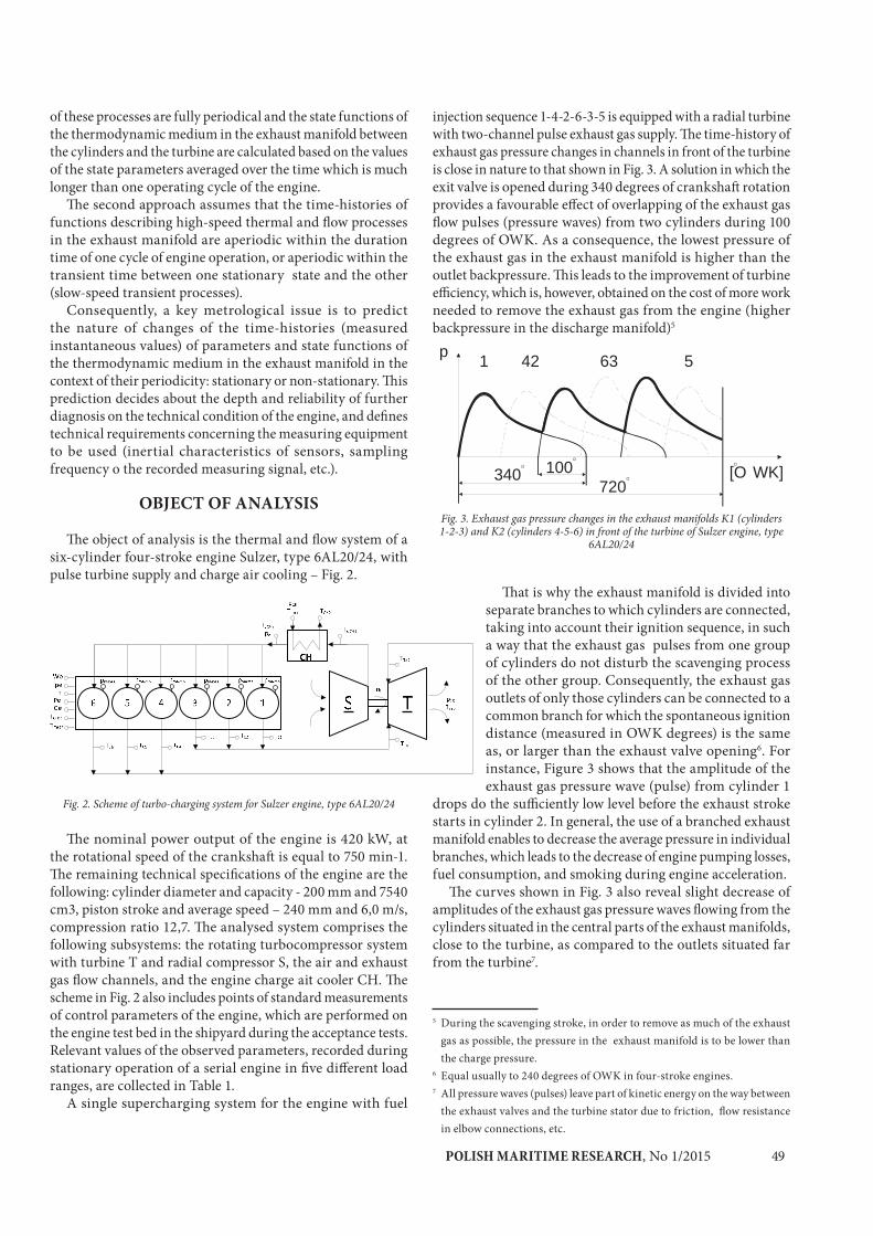
POLISH MARITIME RESEARCH, No 1/2015 49
of these processes are fully periodical and the state functions of the thermodynamic medium in the exhaust manifold between the cylinders and the turbine are calculated based on the values of the state parameters averaged over the time which is much longer than one operating cycle of the engine.
The second approach assumes that the time-histories of functions describing high-speed thermal and flow processes in the exhaust manifold are aperiodic within the duration time of one cycle of engine operation, or aperiodic within the transient time between one stationary state and the other (slow-speed transient processes).
Consequently, a key metrological issue is to predict the nature of changes of the time-histories (measured instantaneous values) of parameters and state functions of the thermodynamic medium in the exhaust manifold in the context of their periodicity: stationary or non-stationary. This prediction decides about the depth and reliability of further diagnosis on the technical condition of the engine, and defines technical requirements concerning the measuring equipment to be used (inertial characteristics of sensors, sampling frequency o the recorded measuring signal, etc.).
OBJECT OF ANALYSIS
The object of analysis is the thermal and flow system of a six-cylinder four-stroke engine Sulzer, type 6AL20/24, with pulse turbine supply and charge air cooling – Fig. 2.
Fig. 2. Scheme of turbo-charging system for Sulzer engine, type 6AL20/24
The nominal power output of the engine is 420 kW, at the rotational speed of the crankshaft is equal to 750 min-1. The remaining technical specifications of the engine are the following: cylinder diameter and capacity - 200 mm and 7540 cm3, piston stroke and average speed – 240 mm and 6,0 m/s, compression ratio 12,7. The analysed system comprises the following subsystems: the rotating turbocompressor system with turbine T and radial compressor S, the air and exhaust gas flow channels, and the engine charge ait cooler CH. The scheme in Fig. 2 also includes points of standard measurements of control parameters of the engine, which are performed on the engine test bed in the shipyard during the acceptance tests. Relevant values of the observed parameters, recorded during stationary operation of a serial engine in five different load ranges, are collected in Table 1.
A single supercharging system for the engine with fuel
injection sequence 1-4-2-6-3-5 is equipped with a radial turbine with two-channel pulse exhaust gas supply. The time-history of exhaust gas pressure changes in channels in front of the turbine is close in nature to that shown in Fig. 3. A solution in which the exit valve is opened during 340 degrees of crankshaft rotation provides a favourable effect of overlapping of the exhaust gas flow pulses (pressure waves) from two cylinders during 100 degrees of OWK. As a consequence, the lowest pressure of the exhaust gas in the exhaust manifold is higher than the outlet backpressure. This leads to the improvement of turbine efficiency, which is, however, obtained on the cost of more work needed to remove the exhaust gas from the engine (higher backpressure in the discharge manifold)5
Fig. 3. Exhaust gas pressure changes in the exhaust manifolds K1 (cylinders 1-2-3) and K2 (cylinders 4-5-6) in front of the turbine of Sulzer engine, type
6AL20/24
That is why the exhaust manifold is divided into separate branches to which cylinders are connected, taking into account their ignition sequence, in such a way that the exhaust gas pulses from one group of cylinders do not disturb the scavenging process of the other group. Consequently, the exhaust gas outlets of only those cylinders can be connected to a common branch for which the spontaneous ignition distance (measured in OWK degrees) is the same as, or larger than the exhaust valve opening6. For instance, Figure 3 shows that the amplitude of the exhaust gas pressure wave (pulse) from cylinder 1
drops do the sufficiently low level before the exhaust stroke starts in cylinder 2. In general, the use of a branched exhaust manifold enables to decrease the average pressure in individual branches, which leads to the decrease of engine pumping losses, fuel consumption, and smoking during engine acceleration.
The curves shown in Fig. 3 also reveal slight decrease of amplitudes of the exhaust gas pressure waves flowing from the cylinders situated in the central parts of the exhaust manifolds, close to the turbine, as compared to the outlets situated far from the turbine7.
5 During the scavenging stroke, in order to remove as much of the exhaust gas as possible, the pressure in the exhaust manifold is to be lower than the charge pressure.
6 Equal usually to 240 degrees of OWK in four-stroke engines.7 All pressure waves (pulses) leave part of kinetic energy on the way between
the exhaust valves and the turbine stator due to friction, flow resistance in elbow connections, etc.
1
340O 100
O
720O
p
[O WK]O
42 63 5
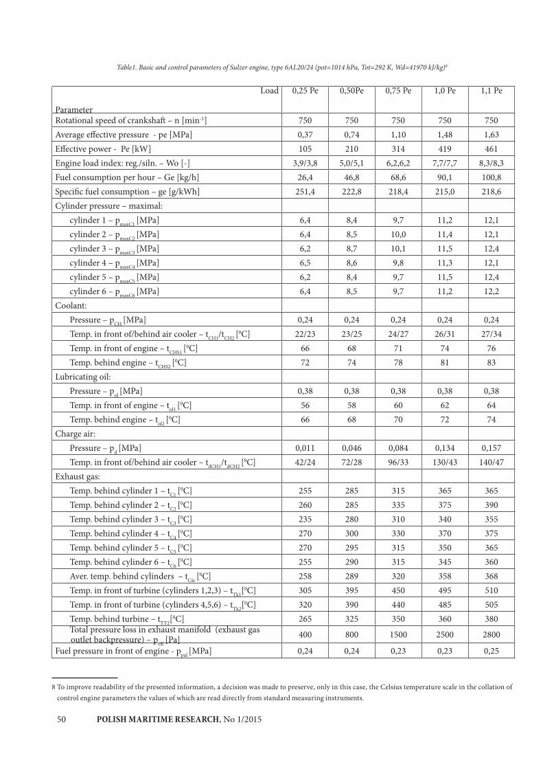
POLISH MARITIME RESEARCH, No 1/201550
Table1. Basic and control parameters of Sulzer engine, type 6AL20/24 (pot=1014 hPa, Tot=292 K, Wd=41970 kJ/kg)8
8 To improve readability of the presented information, a decision was made to preserve, only in this case, the Celsius temperature scale in the collation of control engine parameters the values of which are read directly from standard measuring instruments.
Load
Parameter
0,25 Pe 0,50Pe 0,75 Pe 1,0 Pe 1,1 Pe
Rotational speed of crankshaft – n [min-1] 750 750 750 750 750Average effective pressure - pe [MPa] 0,37 0,74 1,10 1,48 1,63Effective power - Pe [kW] 105 210 314 419 461Engine load index: reg./siln. – Wo [-] 3,9/3,8 5,0/5,1 6,2,6,2 7,7/7,7 8,3/8,3Fuel consumption per hour – Ge [kg/h] 26,4 46,8 68,6 90,1 100,8Specific fuel consumption – ge [g/kWh] 251,4 222,8 218,4 215,0 218,6Cylinder pressure – maximal: cylinder 1 – pmaxC1 [MPa] 6,4 8,4 9,7 11,2 12,1 cylinder 2 – pmaxC2 [MPa] 6,4 8,5 10,0 11,4 12,1 cylinder 3 – pmaxC3 [MPa] 6,2 8,7 10,1 11,5 12,4 cylinder 4 – pmaxC4 [MPa] 6,5 8,6 9,8 11,3 12,1 cylinder 5 – pmaxC5 [MPa] 6,2 8,4 9,7 11,5 12,4 cylinder 6 – pmaxC6 [MPa] 6,4 8,5 9,7 11,2 12,2Coolant: Pressure – pCH [MPa] 0,24 0,24 0,24 0,24 0,24 Temp. in front of/behind air cooler – tCH1/tCH2 [0C] 22/23 23/25 24/27 26/31 27/34 Temp. in front of engine – tCHS1 [0C] 66 68 71 74 76 Temp. behind engine – tCHS2 [0C] 72 74 78 81 83Lubricating oil: Pressure – pol [MPa] 0,38 0,38 0,38 0,38 0,38 Temp. in front of engine – tol1 [0C] 56 58 60 62 64 Temp. behind engine – tol2 [0C] 66 68 70 72 74Charge air: Pressure – pd [MPa] 0,011 0,046 0,084 0,134 0,157 Temp. in front of/behind air cooler – tdCH1/tdCH2 [0C] 42/24 72/28 96/33 130/43 140/47Exhaust gas: Temp. behind cylinder 1 – tC1 [0C] 255 285 315 365 365 Temp. behind cylinder 2 – tC2 [0C] 260 285 335 375 390 Temp. behind cylinder 3 – tC3 [0C] 235 280 310 340 355 Temp. behind cylinder 4 – tC4 [0C] 270 300 330 370 375 Temp. behind cylinder 5 – tC5 [0C] 270 295 315 350 365 Temp. behind cylinder 6 – tC6 [0C] 255 290 315 345 360 Aver. temp. behind cylinders – tCśr [0C] 258 289 320 358 368 Temp. in front of turbine (cylinders 1,2,3) – tTk1[0C] 305 395 450 495 510 Temp. in front of turbine (cylinders 4,5,6) – tTk2[0C] 320 390 440 485 505 Temp. behind turbine – tTT2[0C] 265 325 350 360 380 Total pressure loss in exhaust manifold (exhaust gas
outlet backpressure) – pcK [Pa] 400 800 1500 2500 2800
Fuel pressure in front of engine - ppal [MPa] 0,24 0,24 0,23 0,23 0,25
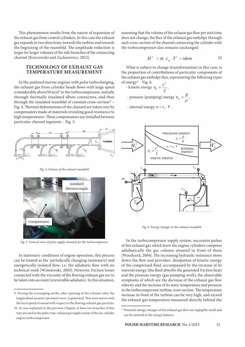
POLISH MARITIME RESEARCH, No 1/2015 51
This phenomenon results from the nature of expansion of the exhaust gas from central cylinders. In this case the exhaust gas expands in two directions: towards the turbine and towards the beginning of the manifold. The amplitude reduction is larger for larger volumes of the side branches of the connecting channel [Korczewski and Zacharewicz, 2012].
TECHNOLOGY OF EXHAUST GAS TEMPERATURE MEASUREMENT
In the analysed marine engines with pulse turbocharging, the exhaust gas from cylinder heads flows with large speed (considerably above50 m/s)9 to the turbocompressor, initially through thermally insulated elbow connectors, and then through the insulated manifold of constant cross-section10 – Fig. 4. Thermal deformations of the channel are taken over by compensators made of materials revealing good resistance to high temperatures. These compensators are installed between particular channel segments – Fig. 5.
Fig. 4. Scheme of the exhaust manifold
Fig. 5. General view of pulse supply channels for the turbocompressor
In stationary conditions of engine operation, this process can be treated as the periodically changing (stationary) and energetically isolated flow, i.e. the adiabatic flow with no technical work [Wiśniewski, 2005]. However, friction losses connected with the viscosity of the flowing exhaust gas are to be taken into account (irreversible adiabatic). In this situation,
9 During the scavenging stroke, after opening of the exhaust valve the longitudinal acoustic (pressure) wave is generated. This wave moves with the local speed of sound with respect to the flowing exhaust gas particles.
10 As was explained in the previous Chapter, at least two branches of this type are used in the pulse-type exhaust gas supply system of the six-cylinder engine turbocompressor.
assuming that the volume of the exhaust gas flow per unit time does not change, the flux of the exhaust gas enthalpy through each cross-section of the channel connecting the cylinder with the turbocompressor also remains unchanged:
(1)
What is subject to change (transformation) in this case, is the proportion of contributions of particular components of the exhaust gas enthalpy flux, representing the following types of energy11 - Fig. 6:
- kinetic energy 2
2cek ,
- pressure (pumping) energy pep ,
- internal energy Tcu v .
Fig. 6. Energy changes in the exhaust manifold
In the turbocompressor supply system, successive pulses of hot exhaust gas which leave the engine cylinders compress adiabatically the gas column situated in front of them [Woodyard, 2004]. The increasing hydraulic resistance slows down the flow and provokes dissipation of kinetic energy of the compressed fluid, accompanied by the increase of its internal energy (the fluid absorbs the generated friction heat) and the pressure energy (gas pumping work), the observable symptoms of which are the decrease of the exhaust gas flow velocity and the increase of its static temperature and pressure in the turbocompressor turbine cross-section. The temperature increase in front of the turbine can be very high, and exceed the exhaust gas temperature measured directly behind the
11 Potential energy changes of the exhaust gas flow are negligibly small and can be omitted in the energy balance.
1CT2TTT2CT 3CT
1TkT
compensator
standard thermocouple
idemTcmH p
a
Tc1TTk1
TTT2
pw
nn
cco
1
2
c
c t
KINETIC ENERGY
INTERNAL ENERGY
PRESSURE ENERGY
gpep
2
2cek
Tcu v1H 2H
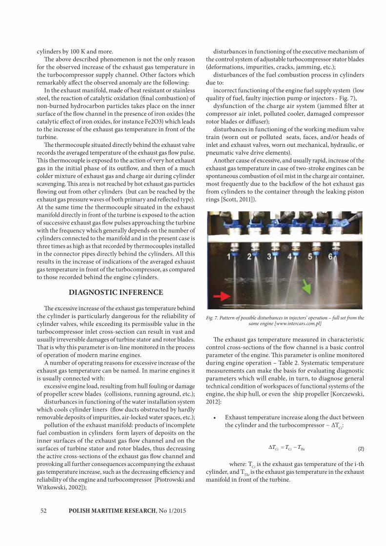
POLISH MARITIME RESEARCH, No 1/201552
cylinders by 100 K and more. The above described phenomenon is not the only reason
for the observed increase of the exhaust gas temperature in the turbocompressor supply channel. Other factors which remarkably affect the observed anomaly are the following:
In the exhaust manifold, made of heat resistant or stainless steel, the reaction of catalytic oxidation (final combustion) of non-burned hydrocarbon particles takes place on the inner surface of the flow channel in the presence of iron oxides (the catalytic effect of iron oxides, for instance Fe2O3) which leads to the increase of the exhaust gas temperature in front of the turbine.
The thermocouple situated directly behind the exhaust valve records the averaged temperature of the exhaust gas flow pulse. This thermocouple is exposed to the action of very hot exhaust gas in the initial phase of its outflow, and then of a much colder mixture of exhaust gas and charge air during cylinder scavenging. This area is not reached by hot exhaust gas particles flowing out from other cylinders (but can be reached by the exhaust gas pressure waves of both primary and reflected type). At the same time the thermocouple situated in the exhaust manifold directly in front of the turbine is exposed to the action of successive exhaust gas flow pulses approaching the turbine with the frequency which generally depends on the number of cylinders connected to the manifold and in the present case is three times as high as that recorded by thermocouples installed in the connector pipes directly behind the cylinders. All this results in the increase of indications of the averaged exhaust gas temperature in front of the turbocompressor, as compared to those recorded behind the engine cylinders.
DIAGNOSTIC INFERENCE
The excessive increase of the exhaust gas temperature behind the cylinder is particularly dangerous for the reliability of cylinder valves, while exceeding its permissible value in the turbocompressor inlet cross-section can result in vast and usually irreversible damages of turbine stator and rotor blades. That is why this parameter is on-line monitored in the process of operation of modern marine engines.
A number of operating reasons for excessive increase of the exhaust gas temperature can be named. In marine engines it is usually connected with:
excessive engine load, resulting from hull fouling or damage of propeller screw blades (collisions, running aground, etc.);
disturbances in functioning of the water installation system which cools cylinder liners (flow ducts obstructed by hardly removable deposits of impurities, air-locked water spaces, etc.);
pollution of the exhaust manifold: products of incomplete fuel combustion in cylinders form layers of deposits on the inner surfaces of the exhaust gas flow channel and on the surfaces of turbine stator and rotor blades, thus decreasing the active cross-sections of the exhaust gas flow channel and provoking all further consequences accompanying the exhaust gas temperature increase, such as the decreasing efficiency and reliability of the engine and turbocompressor [Piotrowski and Witkowski, 2002]);
disturbances in functioning of the executive mechanism of the control system of adjustable turbocompressor stator blades (deformations, impurities, cracks, jamming, etc.);
disturbances of the fuel combustion process in cylinders due to:
incorrect functioning of the engine fuel supply system (low quality of fuel, faulty injection pump or injectors - Fig. 7),
dysfunction of the charge air system (jammed filter at compressor air inlet, polluted cooler, damaged compressor rotor blades or diffuser);
disturbances in functioning of the working medium valve train (worn out or polluted seats, faces, and/or heads of inlet and exhaust valves, worn out mechanical, hydraulic, or pneumatic valve drive elements).
Another cause of excessive, and usually rapid, increase of the exhaust gas temperature in case of two-stroke engines can be spontaneous combustion of oil mist in the charge air container, most frequently due to the backflow of the hot exhaust gas from cylinders to the container through the leaking piston rings [Scott, 2011]).
Fig. 7. Pattern of possible disturbances in injectors’ operation – full set from the same engine [www.intercars.com.pl]
The exhaust gas temperature measured in characteristic control cross-sections of the flow channel is a basic control parameter of the engine. This parameter is online monitored during engine operation – Table 2. Systematic temperature measurements can make the basis for evaluating diagnostic parameters which will enable, in turn, to diagnose general technical condition of workspaces of functional systems of the engine, the ship hull, or even the ship propeller [Korczewski, 2012]:
• Exhaust temperature increase along the duct between the cylinder and the turbocompressor − ΔTCi:
TkiCiCi TTT (2)
where: TCi is the exhaust gas temperature of the i-th cylinder, and TTki is the exhaust gas temperature in the exhaust manifold in front of the turbine.
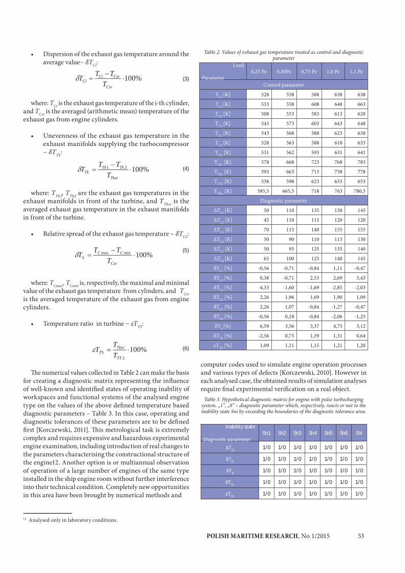
POLISH MARITIME RESEARCH, No 1/2015 53
• Dispersion of the exhaust gas temperature around the average value− δTCi:
%100Csr
CsrCiCi T
TTT (3)
where: TCi is the exhaust gas temperature of the i-th cylinder,
and TCsr is the averaged (arithmetic mean) temperature of the exhaust gas from engine cylinders.
• Unevenness of the exhaust gas temperature in the exhaust manifolds supplying the turbocompressor − δTTk:
%10021
Tksr
TkTkTk T
TTT (4)
where: TTk1, TTk2 are the exhaust gas temperatures in the
exhaust manifolds in front of the turbine, and TTksr is the averaged exhaust gas temperature in the exhaust manifolds in front of the turbine.
• Relative spread of the exhaust gas temperature − δTCS:
%100minmax
Csr
CCS T
TTT
(5)
where: TCmax, TCmin is, respectively, the maximal and minimal value of the exhaust gas temperature from cylinders, and TCsr is the averaged temperature of the exhaust gas from engine cylinders.
• Temperature ratio in turbine − εTTS:
%1002TT
TksrTS T
TT (6)
The numerical values collected in Table 2 can make the basis for creating a diagnostic matrix representing the influence of well-known and identified states of operating inability of workspaces and functional systems of the analysed engine type on the values of the above defined temperature based diagnostic parameters – Table 3. In this case, operating and diagnostic tolerances of these parameters are to be defined first [Korczewski, 2011]. This metrological task is extremely complex and requires expensive and hazardous experimental engine examination, including introduction of real changes to the parameters characterising the constructional structure of the engine12. Another option is or multiannual observation of operation of a large number of engines of the same type installed in the ship engine room without further interference into their technical condition. Completely new opportunities in this area have been brought by numerical methods and
12 Analysed only in laboratory conditions.
Table 2. Values of exhaust gas temperature treated as control and diagnostic parameter
Load
Parameter0,25 Pe 0,50Pe 0,75 Pe 1,0 Pe 1,1 Pe
Control parameter
TC1 [K] 528 558 588 638 638
TC2 [K] 533 558 608 648 663
TC3 [K] 508 553 583 613 628
TC4 [K] 543 573 603 643 648
TC5 [K] 543 568 588 623 638
TC6 [K] 528 563 588 618 633
TCśr [K] 531 562 593 631 641
TTk1 [K] 578 668 723 768 783
TTk2 [K] 593 663 713 758 778
TTT2 [K] 538 598 623 633 653
TTkśr [K] 585,5 665,5 718 763 780,5
Diagnostic parameter
ΔTC1 [K] 50 110 135 130 145
ΔTC2 [K] 45 110 115 120 120
ΔTC3 [K] 70 115 140 155 155
ΔTC4 [K] 50 90 110 115 130
ΔTC5 [K] 50 95 125 135 140
ΔTC6 [K] 65 100 125 140 145
δTC1 [%] -0,56 -0,71 -0,84 1,11 -0,47
δTC2 [%] 0,38 -0,71 2,53 2,69 3,43
δTC3 [%] -4,33 -1,60 -1,69 -2,85 -2,03
δTC4 [%] 2,26 1,96 1,69 1,90 1,09
δTC5 [%] 2,26 1,07 -0,84 -1,27 -0,47
δTC6 [%] -0,56 0,18 -0,84 -2,06 -1,25
δTS [%] 6,59 3,56 3,37 4,75 3,12
δTTk [%] -2,56 0,75 1,39 1,31 0,64
εTTS [%] 1,09 1,11 1,15 1,21 1,20
computer codes used to simulate engine operation processes and various types of defects [Korczewski, 2010]. However in each analysed case, the obtained results of simulation analyses require final experimental verification on a real object.
Table 3. Hypothetical diagnostic matrix for engine with pulse turbocharging system. „1”, „0” – diagnostic parameter which, respectively, reacts or not to the inability state Sni by exceeding the boundaries of the diagnostic tolerance area.
Inability state Sn1 Sn2 Sn3 Sn4 Sn5 Sn6 Sni
Ci 1/0 1/0 1/0 1/0 1/0 1/0 1/0
Ci 1/0 1/0 1/0 1/0 1/0 1/0 1/0
S 1/0 1/0 1/0 1/0 1/0 1/0 1/0
1/0 1/0 1/0 1/0 1/0 1/0 1/0
1/0 1/0 1/0 1/0 1/0 1/0 1/0

POLISH MARITIME RESEARCH, No 1/201554
FINAL REMARKS AND CONCLUSIONS
The article presents opportunities for making general evaluation of technical condition of a marine ship with pulse turbocharging system based on standard exhaust gas temperature measurements performed in characteristic control cross-sections of the thermal and flow systems of the engine, in stationary conditions of ship motor system operation. This evaluation makes the basis for further more detailed diagnostic analyses, provided that the time-histories of functions describing high-speed thermal and flow processes in the exhaust manifold are aperiodic within the time duration of one cycle of engine operation. This approach requires working out a new technology of on-line measurements of instantaneous values of the exhaust gas temperature in the channel connecting the cylinders with the turbocompressor, in order to determine precisely the nature of enthalpy flux changes of the exhaust gas supplying the turbocompressor.
BIBLIOGRAPHY
1. Korczewski Z.: An entropy function application within the selection process of diagnostic parameters of marine diesel and gas turbine engines. Polish Maritime Research, 2(65)/2010, Vol.17, p. 29-35.
2. Korczewski Z.: Exhaust gas temperature measurements in diagnostic examination of naval gas turbine engines. Part III. Diagnostic and operating tolerances. Polish Maritime Research, No. 4(71)/2011, Vol.18, p. 49-53.
3. Korczewski Z.: Analysing possible use of the diagnostic model of internal combustion engine piston-crankshaft systems and evaluating its practical applicability to rational control of the process of their operation taking into account the expert system (in Polish). Work within the framework of the Research Project No. N509 494638 financed by MNiSW. Gdansk University of Technology, 2012.
4. Korczewski Z., Zacharewicz M.: Alternative diagnostic method applied on marine diesel engines having limited monitoring susceptibility. Transactions of the Institute of Measurement and Control, Great Britain SAGE - Vol. 34, No. 8/December/2012, 2012, p. 937-946.
5. Kluj S.: Diagnostics of marine equipment (in Polish). Monographic publication. AM Gdynia 2000.
6. Pfriem, H.: Zur messung vernderlicher temperaturen von gasen und flssigkeiten (On the measurement of fluctuating temperatures of gases and fluids). Forschung auf dem Gebiete des Ingenieurwesens,7(2)/1936, pp. 85-92 (in German).
7. Piotrowski I., Witkowski K.: Operation of marine internal combustion engines (in Polish). Monographic publication.
Gdynia Maritime Academy, Gdynia 2002.
8. Rychter T., Teodorczyk A.: Theory of piston engines (in Polish). WKiŁ, Warszawa 2006.
9. Scott W.: Diagnosing Causes of High EGT in Marine Engines. Marine Machinery, Engines & Controls. Edited by Lamar Stonecypher (updated: 11/2/2011).
10. Wisłocki K.: Turbocharging systems for high-speed internal combustion engines (in Polish) WKiŁ, Warsaw 1991.
11. Wiśniewski S.: Technical thermodynamics (in Polish). WNT, Warsaw 2005.
12. Wiśniewski S.: Temperature measurements in tests of engines and thermal facilities (in Polish). WNT, Warsaw 1983.
13. Woodyard D.: Pounders marine diesel engines and gas turbine. Great Britain ELSEVIER, 2004 (eighth edition).
14. Wojnowski W.: Marine internal combustion engine power plants (in Polish). Part I. Polish Naval Academy. Gdynia 1998.
15. www.intercars.com.pl
CONTACT WITH THE AUTHOR
Zbigniew Korczewski
Gdańsk University of Technology11/12 Narutowicza St.
80 - 233 GdańskPoland
POLISH MARITIME RESEARCH, No 1/2015 55
POLISH MARITIME RESEARCH 1(85) 2015 Vol. 22; pp. 55-6410.1515/pomr-2015-0008
APPLICATION ISSSUES OF THE SEMI-MARKOV RELIABILITY MODEL
Jacek Rudnicki, Ph. D.Gdańsk Univeristy of Technology, Poland
ABSTRACT
Predicting the reliability of marine internal combustion engines, for instance, is of particular importance, as it makes it possible to predict their future reliability states based on the information on the past states. Correct reliability prediction is a complex process which consists in processing empirical results obtained from operating practice, complemented by analytical considerations. The process of technical state changes of each mechanical device is stochastic and continuous in states and time, hence the need to divide this infinite set of engine states into a finite number of subsets (classes), which can be clearly and permanently identified using the existing diagnosing system. Using the engine piston-crankshaft system as an example, the article presents a proposal for a mathematical model of reliability which, on the one hand, takes into account random nature of phenomena leading to the damage, and at the same time reveals certain application flexibility and the resultant practical usability.
Keywords: service speed, shipping lines, preliminary design
INTRODUCTION
The piston-crankshaft system is functionally one of most important subsystems in the engine, and its importance is additionally increased by the fact that all maintenance activities concerning particular components of this system are connected, as a rule, with serious interference into the engine structure and its long lasting shutdown. Thus the state of the piston-crankshaft system is crucial for the reliability and overall performance of the engine.
During engine operation, its elements are exposed to degradation excitations, which leads to their wear (see: tribological systems of the engine, for instance). This wear, in turn, affects the work process and performance parameters. In the analysed functional system three structural nodes can be named, the technical state of which affects decisively the abovementioned parameters, as well as the general technical state and reliability of the engine. These nodes are: the piston rings-cylinder liner node, the piston-cylinder liner node, and the crosshead, crankshaft and main bearings.
In general, the effect of gradual wear of piston-crankshaft system elements on parameters of the work process can manifest itself in three ways, i.e. as [6]:
• decrease of final parameters of charge compression in the cylinder (pressure and temperature),
• change of conditions of atomisation of the fuel delivered to the cylinder,
• increase of mechanical losses (own resistance) of the engine.
At constant fuel pump setting (hp = const), the increased charge loss caused by decreased piston tightness in the cylinder leads to the decrease of the excess air number ( ). This, in turn, slows down the combustion process, which overlaps the beginning of the decompression stroke and takes place at an increased gas temperature. In the above situation, intensive heat transfer from the wall to the cooling medium and the resultant decrease of the indicated efficiency are observed.
The decrease of the excess air number ( ) and the average indicated pressure (pi) is accompanied by the decrease of the mechanical efficiency ( m), which in turn leads to the decrease of the engine power (Ne).
Moreover, if this phenomenon is accompanied by excessive wear of bearings in the crankshaft system, the piston stroke in the compression process becomes shorter due to summing up of the increased bearing clearances. The final result is the increased volume of combustion chamber and decreased cylinder compression ratio ( ).
Simultaneous action of the charge loss and compression ratio decrease can remarkably affect the indicated efficiency.
The decrease of final compression parameters due to wear of system elements leads to the change of conditions of atomisation and combustion of the fuel delivered to the cylinder. Theoretically, the fuel self-ignition in the cylinder should take place when the combustion temperature becomes equal to the self-ignition temperature. The decrease of the compression pressure and fuel charge density being the result of the lack of piston tightness in the cylinder lead finally to
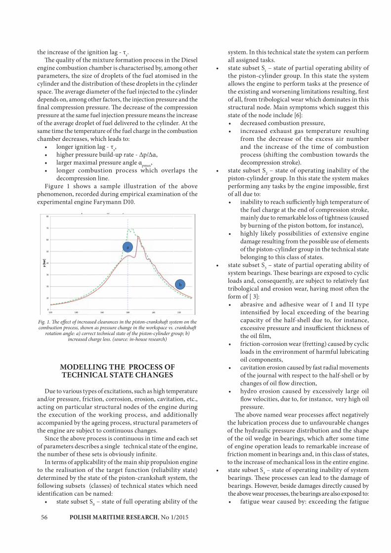
POLISH MARITIME RESEARCH, No 1/201556
the increase of the ignition lag - τs.The quality of the mixture formation process in the Diesel
engine combustion chamber is characterised by, among other parameters, the size of droplets of the fuel atomised in the cylinder and the distribution of these droplets in the cylinder space. The average diameter of the fuel injected to the cylinder depends on, among other factors, the injection pressure and the final compression pressure. The decrease of the compression pressure at the same fuel injection pressure means the increase of the average droplet of fuel delivered to the cylinder. At the same time the temperature of the fuel charge in the combustion chamber decreases, which leads to:
• longer ignition lag - τs,• higher pressure build-up rate - Δp/Δα,• larger maximal pressure angle αpmax,• longer combustion process which overlaps the
decompression line.Figure 1 shows a sample illustration of the above
phenomenon, recorded during empirical examination of the experimental engine Farymann D10.
Fig. 1. The effect of increased clearances in the piston-crankshaft system on the combustion process, shown as pressure change in the workspace vs. crankshaft
rotation angle: a) correct technical state of the piston-cylinder group; b) increased charge loss. (source: in-house research)
MODELLING THE PROCESS OF TECHNICAL STATE CHANGES
Due to various types of excitations, such as high temperature and/or pressure, friction, corrosion, erosion, cavitation, etc., acting on particular structural nodes of the engine during the execution of the working process, and additionally accompanied by the ageing process, structural parameters of the engine are subject to continuous changes.
Since the above process is continuous in time and each set of parameters describes a single technical state of the engine, the number of these sets is obviously infinite.
In terms of applicability of the main ship propulsion engine to the realisation of the target function (reliability state) determined by the state of the piston-crankshaft system, the following subsets (classes) of technical states which need identification can be named:
• state subset S0 – state of full operating ability of the
p g y
a
b
system. In this technical state the system can perform all assigned tasks.
• state subset S1 – state of partial operating ability of the piston-cylinder group. In this state the system allows the engine to perform tasks at the presence of the existing and worsening limitations resulting, first of all, from tribological wear which dominates in this structural node. Main symptoms which suggest this state of the node include [6]:• decreased combustion pressure,• increased exhaust gas temperature resulting
from the decrease of the excess air number and the increase of the time of combustion process (shifting the combustion towards the decompression stroke).
• state subset S2 – state of operating inability of the piston-cylinder group. In this state the system makes performing any tasks by the engine impossible, first of all due to:• inability to reach sufficiently high temperature of
the fuel charge at the end of compression stroke, mainly due to remarkable loss of tightness (caused by burning of the piston bottom, for instance),
• highly likely possibilities of extensive engine damage resulting from the possible use of elements of the piston-cylinder group in the technical state belonging to this class of states.
• state subset S3 – state of partial operating ability of system bearings. These bearings are exposed to cyclic loads and, consequently, are subject to relatively fast tribological and erosion wear, having most often the form of [ 3]:• abrasive and adhesive wear of I and II type
intensified by local exceeding of the bearing capacity of the half-shell due to, for instance, excessive pressure and insufficient thickness of the oil film,
• friction-corrosion wear (fretting) caused by cyclic loads in the environment of harmful lubricating oil components,
• cavitation erosion caused by fast radial movements of the journal with respect to the half-shell or by changes of oil flow direction,
• hydro erosion caused by excessively large oil flow velocities, due to, for instance, very high oil pressure.
The above named wear processes affect negatively the lubrication process due to unfavourable changes of the hydraulic pressure distribution and the shape of the oil wedge in bearings, which after some time of engine operation leads to remarkable increase of friction moment in bearings and, in this class of states, to the increase of mechanical loss in the entire engine.
• state subset S4 – state of operating inability of system bearings. These processes can lead to the damage of bearings. However, beside damages directly caused by the above wear processes, the bearings are also exposed to:• fatigue wear caused by: exceeding the fatigue
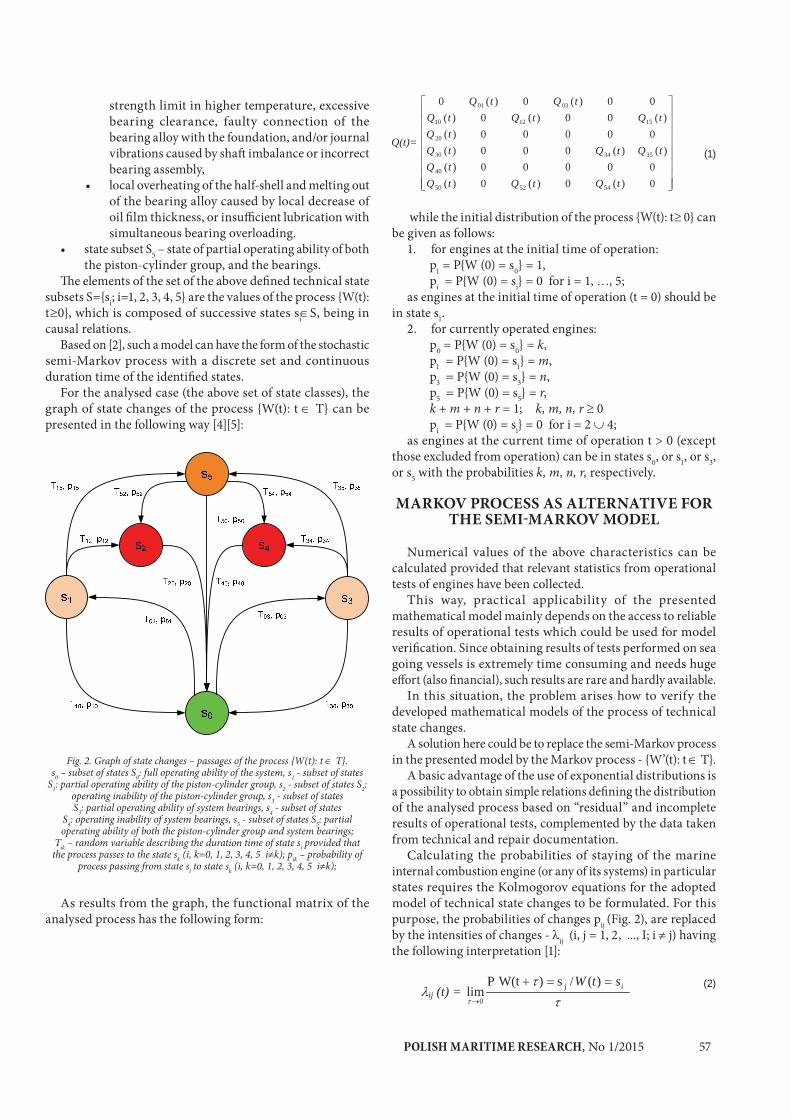
POLISH MARITIME RESEARCH, No 1/2015 57
strength limit in higher temperature, excessive bearing clearance, faulty connection of the bearing alloy with the foundation, and/or journal vibrations caused by shaft imbalance or incorrect bearing assembly,
• local overheating of the half-shell and melting out of the bearing alloy caused by local decrease of oil film thickness, or insufficient lubrication with simultaneous bearing overloading.
• state subset S5 – state of partial operating ability of both the piston-cylinder group, and the bearings.
The elements of the set of the above defined technical state subsets S={si; i=1, 2, 3, 4, 5} are the values of the process {W(t): t≥0}, which is composed of successive states si S, being in causal relations.
Based on [2], such a model can have the form of the stochastic semi-Markov process with a discrete set and continuous duration time of the identified states.
For the analysed case (the above set of state classes), the graph of state changes of the process {W(t): t T} can be presented in the following way [4][5]:
Fig. 2. Graph of state changes – passages of the process {W(t): t T}. s0 – subset of states S0: full operating ability of the system, s1 - subset of states
S1: partial operating ability of the piston-cylinder group, s2 - subset of states S2: operating inability of the piston-cylinder group, s3 - subset of states S3: partial operating ability of system bearings, s4 - subset of states
S4: operating inability of system bearings, s5 - subset of states S5: partial operating ability of both the piston-cylinder group and system bearings;
Tik – random variable describing the duration time of state si provided that the process passes to the state sk (i, k=0, 1, 2, 3, 4, 5 i k); pik – probability of
process passing from state si to state sk (i, k=0, 1, 2, 3, 4, 5 i k);
As results from the graph, the functional matrix of the analysed process has the following form:
(1)
while the initial distribution of the process {W(t): t 0} can be given as follows:
1. for engines at the initial time of operation:p1 = P{W (0) = s0} = 1,pi = P{W (0) = si} = 0 for i = 1, …, 5;
as engines at the initial time of operation (t = 0) should be in state s1.
2. for currently operated engines:p0 = P{W (0) = s0} = k,p1 = P{W (0) = s1} = m,p3 = P{W (0) = s3} = n,p5 = P{W (0) = s5} = r,k + m + n + r = 1; k, m, n, r 0pi = P{W (0) = si} = 0 for i = 2 4;
as engines at the current time of operation t > 0 (except those excluded from operation) can be in states s0, or s1, or s3, or s5 with the probabilities k, m, n, r, respectively.
MARKOV PROCESS AS ALTERNATIVE FOR THE SEMI-MARKOV MODEL
Numerical values of the above characteristics can be calculated provided that relevant statistics from operational tests of engines have been collected.
This way, practical applicability of the presented mathematical model mainly depends on the access to reliable results of operational tests which could be used for model verification. Since obtaining results of tests performed on sea going vessels is extremely time consuming and needs huge effort (also financial), such results are rare and hardly available.
In this situation, the problem arises how to verify the developed mathematical models of the process of technical state changes.
A solution here could be to replace the semi-Markov process in the presented model by the Markov process - {W’(t): t T}.
A basic advantage of the use of exponential distributions is a possibility to obtain simple relations defining the distribution of the analysed process based on “residual” and incomplete results of operational tests, complemented by the data taken from technical and repair documentation.
Calculating the probabilities of staying of the marine internal combustion engine (or any of its systems) in particular states requires the Kolmogorov equations for the adopted model of technical state changes to be formulated. For this purpose, the probabilities of changes pij (Fig. 2), are replaced by the intensities of changes - ij (i, j = 1, 2, ..., I; i j) having the following interpretation [1]:
(2)
0)(0)(0)(00000)(
)()(000)(00000)(
)(00)(0)(00)(0)(0
545250
40
353430
20
151210
0301
tQtQtQtQ
tQtQtQtQ
tQtQtQtQtQ
Q(t)=
ij (t) = istW )(/s)W(tPlim j
0
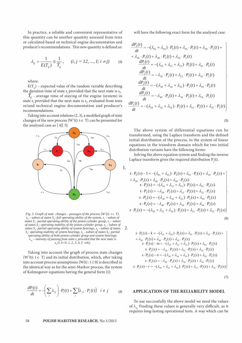
POLISH MARITIME RESEARCH, No 1/201558
In practice, a reliable and convenient representative of this quantity can be another quantity assessed from tests or calculated based on technical engine documentation and producer’s recommendations. This new quantity is defined as:
(3)
where:E(Tij) – expected value of the random variable describing
the duration time of state si provided that the next state is sj,ijT - average time of staying of the engine (system) in
state si provided that the next state is sj, evaluated from tests or/and technical engine documentation and producer’s recommendations.
Taking into account relations (2, 3), a modified graph of state changes of the new process {W’(t): t T} can be presented for the analysed case as [ 4][ 5]:
Fig. 3. Graph of state changes – passages of the process {W’(t): t T}. s0 – subset of states S0: full operating ability of the system, s1 - subset of
states S1: partial operating ability of the piston-cylinder group, s2 - subset of states S2: operating inability of the piston-cylinder group, s3 - subset of states S3: partial operating ability of system bearings, s4 - subset of states S4: operating inability of system bearings, s5 - subset of states S5: partial
operating ability of both piston-cylinder group and system bearings; ik – intensity of passing from state si provided that the next state is
sk (i, k=0, 1, 2, 3, 4, 5 i k);
Taking into account the graph of process state changes {W’(t): t T} and its initial distribution, which, after taking into account process assumptions {W(t) : t 0} is described in the identical way as for the semi-Markov process, the system of Kolmogorov equations having the general form [1]:
(4)
ijijij TTE
1)(
1 , (i, j = 12, ..., I; i j)
will have the following exact form for the analysed case:
(5)
The above system of differential equations can be transformed, using the Laplace transform and the defined initial distribution of the process, to the system of linear equations in the transform domain which for two initial distribution variants have the following forms:
Solving the above equation system and finding the inverse Laplace transform gives the required distribution Pi(t).
(6)
(7)
APPLICATION OF THE RELIABILITY MODEL
To use successfully the above model we need the values of ij. Finding these values is generally very difficult, as it requires long-lasting operational tests. A way which can be
jitPtPdt
tdPj
jjiij
iji )()()(
)()()()()(
)()()()(
)()()()(
)()()()(
)()()()()()()(
)()()()()(
33511555452505
5543344404
00333534303
5521122202
00111512101
550440330
220110003010
tPtPtPdt
tdP
tPtPtPdt
tdP
tPtPdt
tdP
tPtPtPdt
tdP
tPtPdt
tdPtPtPtP
tPtPtPdt
tdP
1.
)()()()()()()()()()()()()()()()()()()()()(
)()()()()()()(1)(
33511555452505
5543344404
00333534303
5521122202
00111512101
550440330
220110003010
sPsPsPsPssPsPsPsPssPsPsPssPsPsPsPssPsPsPs
sPsPsPsPsPsPsPs
2.
)()()()()()()()()(
)()()()()()()()(
)()()()()()()(
)()()()()(
33511555452505
5543344404
00333534303
5521122202
00111512101
550440330
220110003010
sPsPsPrsPssPsPsPsPs
sPsPnsPssPsPsPsPs
sPsPmsPssPsPsP
sPsPsPksPs
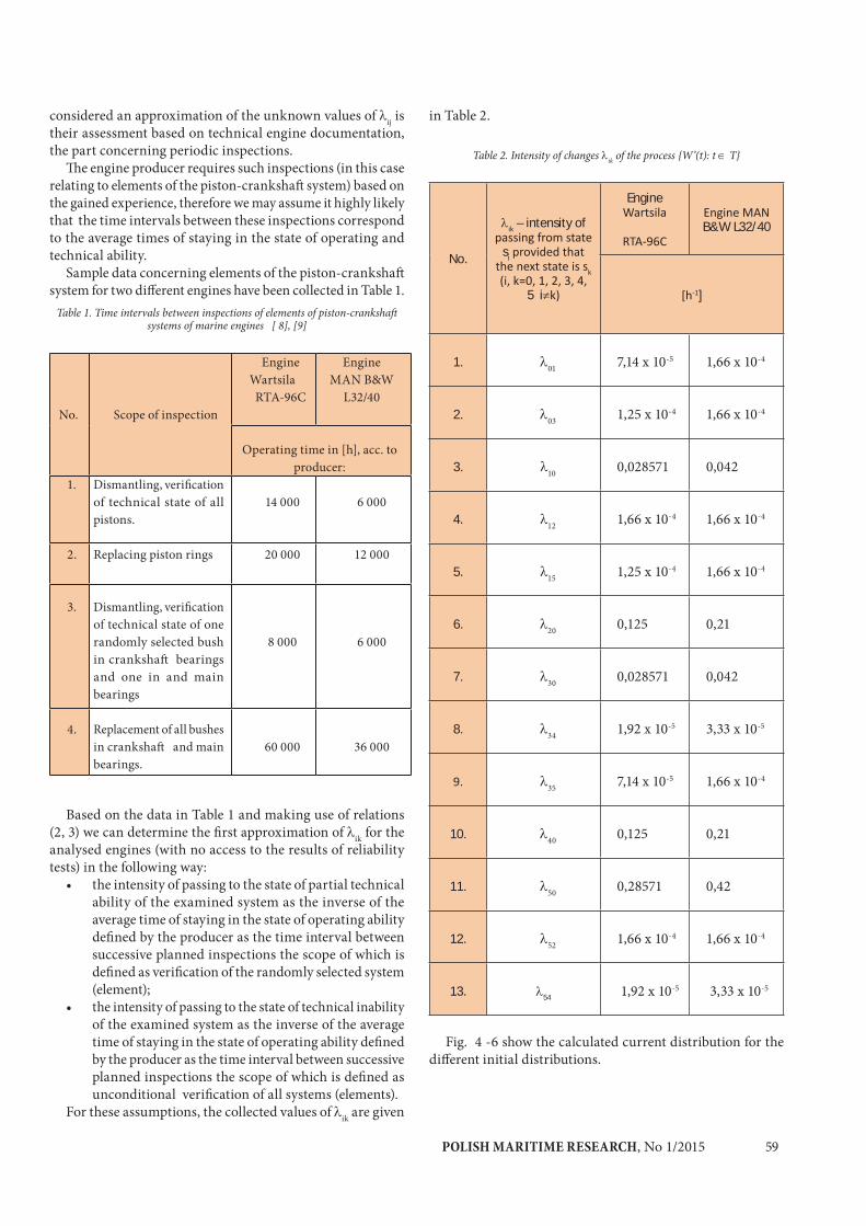
POLISH MARITIME RESEARCH, No 1/2015 59
considered an approximation of the unknown values of ij is their assessment based on technical engine documentation, the part concerning periodic inspections.
The engine producer requires such inspections (in this case relating to elements of the piston-crankshaft system) based on the gained experience, therefore we may assume it highly likely that the time intervals between these inspections correspond to the average times of staying in the state of operating and technical ability.
Sample data concerning elements of the piston-crankshaft system for two different engines have been collected in Table 1.
Table 1. Time intervals between inspections of elements of piston-crankshaft systems of marine engines [ 8], [9]
No. Scope of inspection
Engine WartsilaRTA-96C
Engine MAN B&W
L32/40
Operating time in [h], acc. to producer:
1. Dismantling, verification of technical state of all pistons.
14 000 6 000
2. Replacing piston rings 20 000 12 000
3. Dismantling, verification of technical state of one randomly selected bush in crankshaft bearings and one in and main bearings
8 000 6 000
4. Replacement of all bushes in crankshaft and main bearings.
60 000 36 000
Based on the data in Table 1 and making use of relations (2, 3) we can determine the first approximation of ik for the analysed engines (with no access to the results of reliability tests) in the following way:
• the intensity of passing to the state of partial technical ability of the examined system as the inverse of the average time of staying in the state of operating ability defined by the producer as the time interval between successive planned inspections the scope of which is defined as verification of the randomly selected system (element);
• the intensity of passing to the state of technical inability of the examined system as the inverse of the average time of staying in the state of operating ability defined by the producer as the time interval between successive planned inspections the scope of which is defined as unconditional verification of all systems (elements).
For these assumptions, the collected values of ik are given
in Table 2.
Table 2. Intensity of changes ik of the process {W’(t): t T}
No.
– intensity of
si
5 i
Engine
B&W L32/40
]
1. 01 7,14 x 10⁻⁵ 1,66 x 10⁻⁴
2. 03 1,25 x 10⁻⁴ 1,66 x 10⁻⁴
3. 10 0,028571 0,042
4. 12 1,66 x 10⁻⁴ 1,66 x 10⁻⁴
5. 15 1,25 x 10⁻⁴ 1,66 x 10⁻⁴
6. 20 0,125 0,21
7. 30 0,028571 0,042
8. 34 1,92 x 10⁻⁵ 3,33 x 10⁻⁵
35 7,14 x 10⁻⁵ 1,66 x 10⁻⁴
10. 40 0,125 0,21
11. 50 0,28571 0,42
12. 52 1,66 x 10⁻⁴ 1,66 x 10⁻⁴
13. 54 1,92 x 10⁻⁵ 3,33 x 10⁻⁵
Fig. 4 -6 show the calculated current distribution for the different initial distributions.
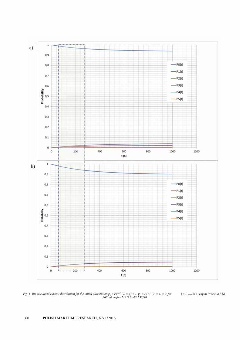
POLISH MARITIME RESEARCH, No 1/201560
Fig. 4. The calculated current distribution for the initial distribution p0 = P{W’ (0) = s0} = 1, pi = P{W’ (0) = si} = 0 for i = 1, …, 5; a) engine Wartsila RTA-96C, b) engine MAN B&W L32/40
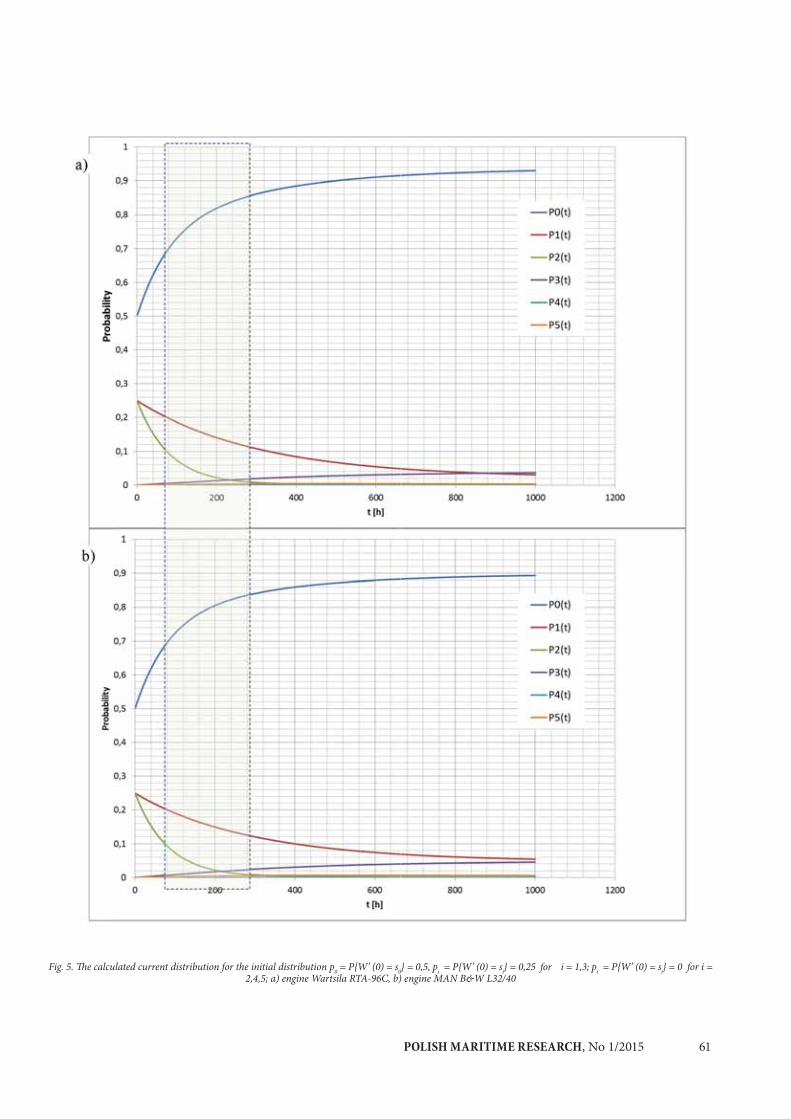
POLISH MARITIME RESEARCH, No 1/2015 61
Fig. 5. The calculated current distribution for the initial distribution p0 = P{W’ (0) = s0} = 0,5, pi = P{W’ (0) = si} = 0,25 for i = 1,3; pi = P{W’ (0) = si} = 0 for i = 2,4,5; a) engine Wartsila RTA-96C, b) engine MAN B&W L32/40
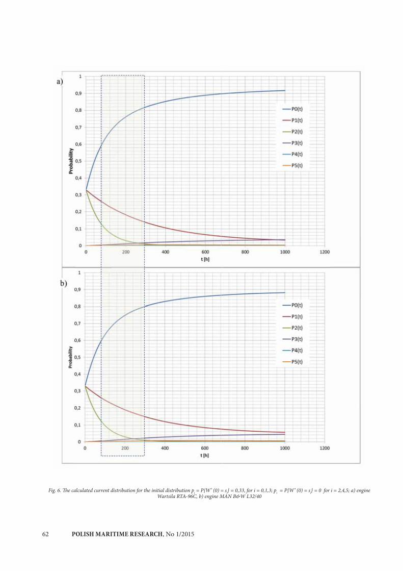
POLISH MARITIME RESEARCH, No 1/201562
Fig. 6. The calculated current distribution for the initial distribution pi = P{W’ (0) = si} = 0,33, for i = 0,1,3; pi = P{W’ (0) = si} = 0 for i = 2,4,5; a) engine Wartsila RTA-96C, b) engine MAN B&W L32/40
POLISH MARITIME RESEARCH, No 1/2015 63
As can be seen in Figs. 4 to 6, from the point of view of decision making a crucial issue for tasks of medium time duration (200 – 300 h) is possibility to identify states s1 and s3 , as the lack of this possibility can result in unjustified decisions, i.e. either overoptimistic (when the assumed initial distribution is p0 = P{W’ (0) = s0} = 1, pi = P{W’ (0) = si} = 0 for i = 1, …, 5), or excessively cautious (when the assumed initial distribution is pi = P{W’ (0) = si} = 0,33, for i = 0,1,3; pi = P{W’ (0) = si} = 0 for i = 2,4,5).
CONCLUSIONS
As the models of real engine operation processes, the semi-Markov processes seem to be more useful than the widely popularised Markov processes. This opinion mainly results from the fact that when analysing processes with continuous time parameter and finite set of states, the intervals of staying of the examined processes in particular states are random variables with arbitrary distributions. This fact makes it possible to take into account, in the developed models, physical aspects of main wear processes being the source of technical state changes. However, practical utilisation of the above models requires, among other features, sufficiently moderate complication level represented by the model, in the sense of a possible smallest number of defined state classes and a relatively simple, in the mathematical sense, functional matrix - Q(t).
This condition is essential when estimating the current distribution pk(t) of process states. This distribution can be calculated based on the known initial distribution of the process and the function pij(t). Calculating the probability pij(t) consists in solving the second-order Voltera equation system in which the know quantities are the functions Qij(t) being the elements of the functional matrix Q(t) of the process. When the number of process states is small and the functional matrix of this process is relatively simple, the system can be solved in the operator domain using the Laplace transform. On the other hand, when the number of states is large or its functional matrix (kernel of the process) is very complex, the equation system can only be solved numerically. This solution does not provide an answer to a question which is very important for operating practice, namely: how will the probabilities of states of the semi-Markov process change when t is large.
It results from the theory of semi-Markov processes that in case of ergodic semi-Markov processes the above probabilities tend with time to precisely defined constant numbers [3, 4]. These numbers bear the names of limiting probabilities of states, and the sequence of these numbers composes the limiting distribution of the process. The limiting distribution can be calculated much more easily than the current distribution, and it enables to define the readiness coefficient, of an engine for instance, and the income or cost per unit time of operation. These quantities, in turn, can be criterial functions when solving engine operation optimisation problems.
However, when the graph of state changes – passages is relatively complicated, a possibility appears to assess the searched probability values by developing the model of the process {W(t) : t 0} in the form of the Markov process - {W’(t): t T}.
Such models represent some simplification of the semi-Markov models. The difference between the Markov process and the semi-Markov process is that in the former process the intervals in which the process stays unconditionally in particular states and the intervals of time duration of a given process state provided that then next state is one of the remaining states of this process are random variables with exponential distribution [1]. This situation limits the use of these processes, but in case of the above described difficulties in working out the semi-Markov model or when the analysed random variables have unknown distributions, the results obtained using the Markov process can be considered the first approximation.
The use of exponential distributions make it possible to obtain very simple relations constituting the distribution of the analysed process.
REFERENCES
1. Benjamin J.R., Cornell C.A.: Probability theory, mathematical statistics, and decision making theory for engineers (in Polish). WNT, Warszawa 1977.
2. Girtler J.: The semi-Markov model of the process of appearance of sea-going ship propulsion system ability and inability states in application to determining the reliability of these systems. Polish Maritime Research. Volume 20, Issue 4, Pages 18–24, 2013.
3. Girtler J.: The semi-Markov model of energy state changes of the main marine internal combustion engine and method for evaluating its operation during ship voyage. Polish Maritime Research. Volume 18, Issue 4, Pages 36–42, 2011.
4. Grabski F.: Theory of semi-Markov processes of operation of technical objects (in Polish). Zeszyty Naukowe AMW, nr 75A, Gdynia 1982.
5. Piaseczny L.: Technology of repairs of marine internal combustion engines (in Polish). Wydawnictwo Morskie, Gdansk 1992.
6. Rudnicki J.: Preparing a collection of technical and energy states of engine piston-crankshaft systems taking place during engine operation (in Polish). Work done within the framework of the project finances by MNiSW. The research project entitled : „Decision making based control of the process of operation of piston-crankshaft systems in Diesel engines used as main propulsion of sea going vessels, making use of technical diagnostics and taking into account safety and marine environment protection. Gdansk 2010.
7. Rudnicki J.: Formulating requirements concerning operating properties of the diagnostic system for ship main engines, with particular attention focused on the

POLISH MARITIME RESEARCH, No 1/201564
technical state of their piston-crankshaft systems, adapted to control the process of operation of this type of engines in the aspect of ship safety and marine environment protection (in Polish) . Work done within the framework of the project No. N N509 494638finances by MNiSW. The research project entitled : „Decision making based control of the process of operation of piston-crankshaft systems in Diesel engines used as main propulsion of sea going vessels, making use of technical diagnostics and taking into account safety and marine environment protection. Gdansk 2011.
8. Włodarski J.K.: Operating states of marine internal combustion engines (in Polish), WSM Gdynia 2001.
9. RTA 96CB Electronic Instruction & Manual. Hunday Heavy Industries CO Ltd., Ulsan Korea 2010.
10. L32/40 Electronic Instruction & Manual. Hunday Heavy Industries CO Ltd., Ulsan Korea 2010.
CONTACT WITH THE AUTHOR
Jacek Rudnicki
Gdańsk University of Technology11/12 Narutowicza St.
80 - 233 GdańskPoland
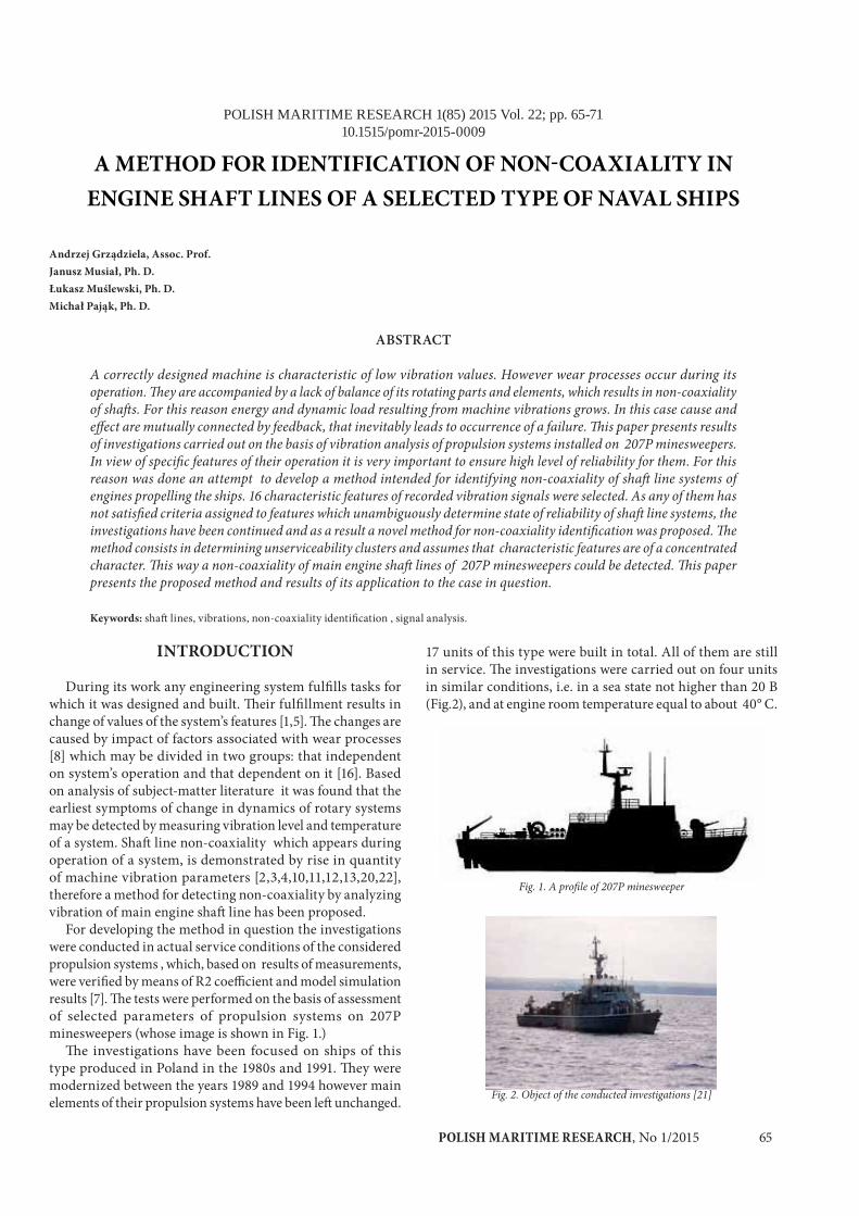
POLISH MARITIME RESEARCH, No 1/2015 65
POLISH MARITIME RESEARCH 1(85) 2015 Vol. 22; pp. 65-7110.1515/pomr-2015-0009
A METHOD FOR IDENTIFICATION OF NON-COAXIALITY IN ENGINE SHAFT LINES OF A SELECTED TYPE OF NAVAL SHIPS
Andrzej Grządziela, Assoc. Prof.Janusz Musiał, Ph. D.Łukasz Muślewski, Ph. D.Michał Pająk, Ph. D.
ABSTRACT
A correctly designed machine is characteristic of low vibration values. However wear processes occur during its operation. They are accompanied by a lack of balance of its rotating parts and elements, which results in non-coaxiality of shafts. For this reason energy and dynamic load resulting from machine vibrations grows. In this case cause and effect are mutually connected by feedback, that inevitably leads to occurrence of a failure. This paper presents results of investigations carried out on the basis of vibration analysis of propulsion systems installed on 207P minesweepers. In view of specific features of their operation it is very important to ensure high level of reliability for them. For this reason was done an attempt to develop a method intended for identifying non-coaxiality of shaft line systems of engines propelling the ships. 16 characteristic features of recorded vibration signals were selected. As any of them has not satisfied criteria assigned to features which unambiguously determine state of reliability of shaft line systems, the investigations have been continued and as a result a novel method for non-coaxiality identification was proposed. The method consists in determining unserviceability clusters and assumes that characteristic features are of a concentrated character. This way a non-coaxiality of main engine shaft lines of 207P minesweepers could be detected. This paper presents the proposed method and results of its application to the case in question.
Keywords: shaft lines, vibrations, non-coaxiality identification , signal analysis.
INTRODUCTION
During its work any engineering system fulfills tasks for which it was designed and built. Their fulfillment results in change of values of the system’s features [1,5]. The changes are caused by impact of factors associated with wear processes [8] which may be divided in two groups: that independent on system’s operation and that dependent on it [16]. Based on analysis of subject-matter literature it was found that the earliest symptoms of change in dynamics of rotary systems may be detected by measuring vibration level and temperature of a system. Shaft line non-coaxiality which appears during operation of a system, is demonstrated by rise in quantity of machine vibration parameters [2,3,4,10,11,12,13,20,22], therefore a method for detecting non-coaxiality by analyzing vibration of main engine shaft line has been proposed.
For developing the method in question the investigations were conducted in actual service conditions of the considered propulsion systems , which, based on results of measurements, were verified by means of R2 coefficient and model simulation results [7]. The tests were performed on the basis of assessment of selected parameters of propulsion systems on 207P minesweepers (whose image is shown in Fig. 1.)
The investigations have been focused on ships of this type produced in Poland in the 1980s and 1991. They were modernized between the years 1989 and 1994 however main elements of their propulsion systems have been left unchanged.
17 units of this type were built in total. All of them are still in service. The investigations were carried out on four units in similar conditions, i.e. in a sea state not higher than 20 B (Fig.2), and at engine room temperature equal to about 40° C.
Fig. 1. A profile of 207P minesweeper
Fig. 2. Object of the conducted investigations [21]
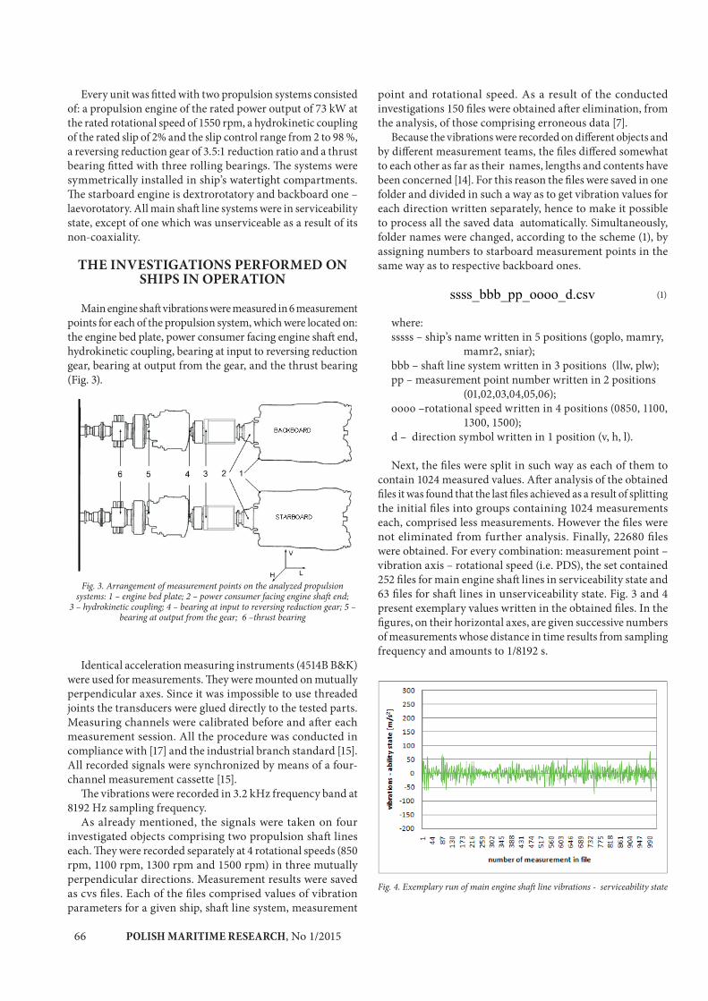
POLISH MARITIME RESEARCH, No 1/201566
Every unit was fitted with two propulsion systems consisted of: a propulsion engine of the rated power output of 73 kW at the rated rotational speed of 1550 rpm, a hydrokinetic coupling of the rated slip of 2% and the slip control range from 2 to 98 %, a reversing reduction gear of 3.5:1 reduction ratio and a thrust bearing fitted with three rolling bearings. The systems were symmetrically installed in ship’s watertight compartments. The starboard engine is dextrorotatory and backboard one – laevorotatory. All main shaft line systems were in serviceability state, except of one which was unserviceable as a result of its non-coaxiality.
THE INVESTIGATIONS PERFORMED ON SHIPS IN OPERATION
Main engine shaft vibrations were measured in 6 measurement points for each of the propulsion system, which were located on: the engine bed plate, power consumer facing engine shaft end, hydrokinetic coupling, bearing at input to reversing reduction gear, bearing at output from the gear, and the thrust bearing (Fig. 3).
Fig. 3. Arrangement of measurement points on the analyzed propulsion systems: 1 – engine bed plate; 2 – power consumer facing engine shaft end;
3 – hydrokinetic coupling; 4 – bearing at input to reversing reduction gear; 5 – bearing at output from the gear; 6 –thrust bearing
Identical acceleration measuring instruments (4514B B&K) were used for measurements. They were mounted on mutually perpendicular axes. Since it was impossible to use threaded joints the transducers were glued directly to the tested parts. Measuring channels were calibrated before and after each measurement session. All the procedure was conducted in compliance with [17] and the industrial branch standard [15]. All recorded signals were synchronized by means of a four-channel measurement cassette [15].
The vibrations were recorded in 3.2 kHz frequency band at 8192 Hz sampling frequency.
As already mentioned, the signals were taken on four investigated objects comprising two propulsion shaft lines each. They were recorded separately at 4 rotational speeds (850 rpm, 1100 rpm, 1300 rpm and 1500 rpm) in three mutually perpendicular directions. Measurement results were saved as cvs files. Each of the files comprised values of vibration parameters for a given ship, shaft line system, measurement
point and rotational speed. As a result of the conducted investigations 150 files were obtained after elimination, from the analysis, of those comprising erroneous data [7].
Because the vibrations were recorded on different objects and by different measurement teams, the files differed somewhat to each other as far as their names, lengths and contents have been concerned [14]. For this reason the files were saved in one folder and divided in such a way as to get vibration values for each direction written separately, hence to make it possible to process all the saved data automatically. Simultaneously, folder names were changed, according to the scheme (1), by assigning numbers to starboard measurement points in the same way as to respective backboard ones.
(1)
where:sssss – ship’s name written in 5 positions (goplo, mamry,
mamr2, sniar); bbb – shaft line system written in 3 positions (llw, plw); pp – measurement point number written in 2 positions
(01,02,03,04,05,06); oooo –rotational speed written in 4 positions (0850, 1100,
1300, 1500); d – direction symbol written in 1 position (v, h, l).
Next, the files were split in such way as each of them to contain 1024 measured values. After analysis of the obtained files it was found that the last files achieved as a result of splitting the initial files into groups containing 1024 measurements each, comprised less measurements. However the files were not eliminated from further analysis. Finally, 22680 files were obtained. For every combination: measurement point – vibration axis – rotational speed (i.e. PDS), the set contained 252 files for main engine shaft lines in serviceability state and 63 files for shaft lines in unserviceability state. Fig. 3 and 4 present exemplary values written in the obtained files. In the figures, on their horizontal axes, are given successive numbers of measurements whose distance in time results from sampling frequency and amounts to 1/8192 s.
Fig. 4. Exemplary run of main engine shaft line vibrations - serviceability state
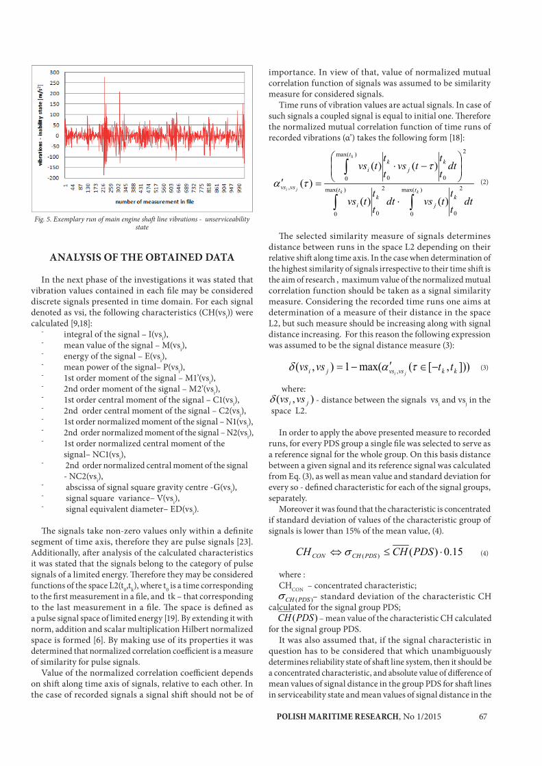
POLISH MARITIME RESEARCH, No 1/2015 67
Fig. 5. Exemplary run of main engine shaft line vibrations - unserviceability state
ANALYSIS OF THE OBTAINED DATA
In the next phase of the investigations it was stated that vibration values contained in each file may be considered discrete signals presented in time domain. For each signal denoted as vsi, the following characteristics (CH(vsi)) were calculated [9,18]:
- integral of the signal – I(vsi),- mean value of the signal – M(vsi),- energy of the signal – E(vsi),- mean power of the signal– P(vsi),- 1st order moment of the signal – M1’(vsi),- 2nd order moment of the signal – M2’(vsi),- 1st order central moment of the signal – C1(vsi),- 2nd order central moment of the signal – C2(vsi),- 1st order normalized moment of the signal – N1(vsi),- 2nd order normalized moment of the signal – N2(vsi),- 1st order normalized central moment of the
signal– NC1(vsi),- 2nd order normalized central moment of the signal
- NC2(vsi),- abscissa of signal square gravity centre -G(vsi),- signal square variance– V(vsi),- signal equivalent diameter– ED(vsi).
The signals take non-zero values only within a definite segment of time axis, therefore they are pulse signals [23]. Additionally, after analysis of the calculated characteristics it was stated that the signals belong to the category of pulse signals of a limited energy. Therefore they may be considered functions of the space L2(t0,tk), where t0 is a time corresponding to the first measurement in a file, and tk – that corresponding to the last measurement in a file. The space is defined as a pulse signal space of limited energy [19]. By extending it with norm, addition and scalar multiplication Hilbert normalized space is formed [6]. By making use of its properties it was determined that normalized correlation coefficient is a measure of similarity for pulse signals.
Value of the normalized correlation coefficient depends on shift along time axis of signals, relative to each other. In the case of recorded signals a signal shift should not be of
importance. In view of that, value of normalized mutual correlation function of signals was assumed to be similarity measure for considered signals.
Time runs of vibration values are actual signals. In case of such signals a coupled signal is equal to initial one. Therefore the normalized mutual correlation function of time runs of recorded vibrations (α’) takes the following form [18]:
(2)
The selected similarity measure of signals determines distance between runs in the space L2 depending on their relative shift along time axis. In the case when determination of the highest similarity of signals irrespective to their time shift is the aim of research , maximum value of the normalized mutual correlation function should be taken as a signal similarity measure. Considering the recorded time runs one aims at determination of a measure of their distance in the space L2, but such measure should be increasing along with signal distance increasing. For this reason the following expression was assumed to be the signal distance measure (3):
(3)
where: - distance between the signals vsi and vsj in the
space L2.
In order to apply the above presented measure to recorded runs, for every PDS group a single file was selected to serve as a reference signal for the whole group. On this basis distance between a given signal and its reference signal was calculated from Eq. (3), as well as mean value and standard deviation for every so - defined characteristic for each of the signal groups, separately.
Moreover it was found that the characteristic is concentrated if standard deviation of values of the characteristic group of signals is lower than 15% of the mean value, (4).
(4)
where : CHCON – concentrated characteristic; – standard deviation of the characteristic CH
calculated for the signal group PDS; – mean value of the characteristic CH calculated
for the signal group PDS.It was also assumed that, if the signal characteristic in
question has to be considered that which unambiguously determines reliability state of shaft line system, then it should be a concentrated characteristic, and absolute value of difference of mean values of signal distance in the group PDS for shaft lines in serviceability state and mean values of signal distance in the
POLISH MARITIME RESEARCH, No 1/201568
group PRS for shaft lines in non-serviceability state, should be greater than sum of standard deviations of signals for these two groups. The characteristic is considered unambiguous (5).
(5)
where: CHUE – unambiguous characteristic; CHCON – concentrated characteristic; – standard deviation of the characteristic CH
calculated from PDS group of signals; – mean value of the characteristic CH calculated
from PDS group of signals;PDSIA – PDS group of signals recorded in main engine shaft
line system in unserviceability state PDSA – PDS group of signals recorded in main engine shaft
line system in serviceability state .Number of groups of signals satisfying condition of
concentration and number of group of signals satisfying condition of unambiguity were determined on the basis of calculation results. Tab. 1 contains the results.
Tab. 1. Concentration and unambiguity of characteristics
METHOD FOR NON-COAXIALITY IDENTIFICATION
On the basis of the values presented in Tab. 1 it was found out that among 16 analyzed characteristics only energy and mean power of signal satisfied conditions of concentration and unambiguity. Unfortunately, they satisfy the conditions only partially and therefore they cannot be the only criteria for identification of non-coaxiality of main engine shaft line systems as far as their qualitative, numerically expressed assessment at a given time instance t, is concerned [14].
Analysis of the values contained in Tab. 1 made it possible to distinguish the characteristics which satisfy condition of concentration in a relatively high degree. These are: signal energy, mean power of signal, abscissa of signal square gravity centre, signal square variance and distance from reference signal.
The distinguished characteristics were used for formulation of a method for identification of non-coaxiality in main engine shaft line systems. To this end the files obtained as a result of operational investigations were divided into two groups. The first of them comprised 14212 files (11356 for shaft line systems in serviceability state and 2856 for shaft line systems in unserviceability state) and the second – comprising 7072 files (5644 for shaft line systems in serviceability state and 1428 for shaft line systems in unserviceability state). The first group was used for determination of central point and radius of five-dimensional clusters of serviceability and unserviceability states identified for each of the PDS groups, separately. Coordinates of central points of the clusters were calculated according to the expression (6), and their radiuses – on the basis of the relation (7):
(6)
where : CCPR – central point of the cluster of the reliability state R
for a given PDS group; R – reliability state equivalent to serviceability state and
unserviceability state; – mean value of signal energy calculated for a given PDS
group for the reliability state R; – mean value of mean signal power calculated for a given
PDS group for the reliability state R; – mean value of abscissa of signal square gravity centre
calculated for a given PDS group for the reliability state R; – mean value of square variance calculated for a given
PDS group for the reliability state R; – mean value of distance from reference signal calculated
for a given PDS group for the reliability state R.
(7)
where: CRR – cluster radius for a given PDS group for the reliability
state R;R – reliability state equivalent to serviceability state and
non-serviceability state; – mean value of the characteristic j calculated for the
reliability state R for a given PDS group; (vsi) – the characteristic j calculated for the signal vsi; vsi – a signal which belongs to a given PDS group of the
reliability states R; j – a characteristic which takes values of : signal energy , its
mean power, abscissa of signal square gravity centre, signal square variance or distance from reference signal.
Next, the second-set signals were analyzed. Such signal was defined as that which belongs to serviceability state cluster, if distance between the signal and serviceability cluster central point , calculated from the relation (8), satisfied the condition (9).
POLISH MARITIME RESEARCH, No 1/2015 69
(8)
where: – signal distance from central point of service-
ability state cluster; CCPA – serviceability state cluster central point;vsi – a signal which belongs to a given PDS group of
serviceability state; CHj(CCPA) – value of the characteristic CHj of the
coordinate CCPA; CHj(vsi) – the characteristic j calculated for the signal vsi; j – a characteristic which takes values of: signal energy, its
mean power, abscissa of signal square gravity centre, signal square variance or distance from reference signal.
(9)
where: CRA – radius of serviceability state cluster; – distance between a signal and central point
of serviceability state cluster.
Similarly, such signal was defined as that belonging to unserviceability state cluster, if distance between the signal and unserviceability cluster central point, calculated from the relation (10), satisfied the condition (11):
(10)
where: – signal distance from central point of
unserviceability state cluster; CCPIA – central point of unserviceability state cluster;vsi – a signal which belongs to a given PDS group of
unserviceability state; CHj(CCPIA)- a value of the characteristic CHj of the
coordinate CCPIA; CHj(vsi) - the characteristic j calculated for the signal vsi; j – a characteristic which takes values of : signal energy, its
mean power, abscissa of signal square gravity centre, signal square variance or distance from reference signal.
(11)
where : CRIA – radius of unserviceability state cluster; – distance between a signal and central point
of unserviceability state cluster.
A signal was taken as that confirming serviceability state of main engine shaft line system if it belonged to serviceability state cluster but not to unserviceability state cluster.
According to the same principle a signal was regarded as that confirming unserviceability state of main engine shaft line system if it belonged to unserviceability state cluster but not to serviceability state cluster.
If a signal belonged neither to serviceability state cluster nor to unserviceability state cluster or it belonged to both the clusters simultaneously, then distances between signal in question and central points of the clusters were analyzed (8), (10). A signal was regarded as that confirming serviceability state of main engine shaft line system if the calculated distances satisfied conditions defined by the formula (12). Otherwise signal in question was not regarded as that confirming occurrence of unserviceability state.
(12)
where : – distance between a signal and central point
of serviceability state cluster; – distance between a signal and central point
of unserviceability state cluster.
Tab. 2 shows results of the examination of the second set of signals.
Tab. 2. Effectiveness of the method for non-coaxiality identification
On the basis of analysis of values comprised in Tab. 2 it was found out that the proposed method may reach very high effectiveness in case of the signals recorded in main engine shaft line systems being in unserviceability state. As far as the signals recorded in main engine shaft line systems being in serviceability state are concerned, precision of their identification is lower. Therefore it is suggested to apply the method in question to the assessing of occurrence probability of non-coaxiality in main engine shaft line systems in unserviceability state. The indicated signals should undergo further analyses to exclude those recorded in main engine shaft line systems in serviceability state.
CONCLUSIONS
On the basis of results of the presented investigations it was concluded that :
- out of 16 characteristic features of recorded signals, only energy and mean power of signal satisfies conditions of concentration and unambiguity;
- energy and mean power of signal satisfies the conditions only partially hence they cannot be the only criteria for identification of occurrence of non-coaxiality in main engine shaft line systems;

POLISH MARITIME RESEARCH, No 1/201570
- signal energy, mean power and abscissa of signal square gravity centre , signal square variance and distance from reference signal represent concentrated features and may be used for developing a method for identification of non-coaxiality in main engine shaft line systems;
- effectiveness of the developed method is satisfactory as it amounts to 65% in case of the signals recorded in shaft line systems in serviceability state and to 94% in case of the signals recorded in shaft line systems in unserviceability state;
- it is recommended to apply the method in question to detection of non-coaxiality in main engine shaft line systems;
- the indicated signals should be further analyzed in order to exclude those recorded in main engine shaft line systems being in serviceability state.
BIBLIOGRAPHY
1. Bielawski P.: Diagnostics of marine propeller shafts. Journal of Polish CIMAC Vol. 6 No. 2, 2011, pp.31-40.
2. Cempel Cz.: Vibroacoustic diagnostics of machines (in Polish). PWN, Warszawa, 1989.
3. Charchalis A., Grządziela A.: Diagnosing the shafting of alignment by means vibration measurement. ICSV Congress Garmisch – Partenkirchen, 2000.
4. Dwojak J., Rzepiela M.: Vibration diagnostics of machines and devices ( in Polish). Edition II. Biuro Gamma, Warszawa, 2005.
5. Girtler J.: The semi-Markov model of the process of appearance of sea-going ship propulsion system ability and inability states in application to determining the reliablity of these systems. Polish Maritime Research 4(80) 2013 Vol. 20; pp. 18-24.
6. Górniewicz I., Roman S.: Mathematical analysis for physicists ( in Polish). Uniwersytet Mikołaja Kopernika, Toruń, 2000.
7. Grządziela A., Muślewski Ł.: High quality simulation of the effects of underwater detonation impact. Journal of Vibroengineering, March 2013, Volume 15, Issue 1.
8. Gurr C., Rulfs H.: Influence of transient operating conditions on propeller shaft bearings. Journal of Marine Engineering and Technology, No. 12/2008, pp. 3-7.
9. Izydorczyk J., Pionka G., Tyma G.: Theory of signals . Introduction ( in Polish). 2nd edition - corrected and amended, HELION, Gliwice, 2006.
10. Jarysz-Kamińska E.: Sighting through as part of shaft alignment procedure. Diagnostyka 4(56) 2010, pp. 65-68.
11. Łączkowski R.: Vibroacoustics of machines and devices (in Polish). WNT, Warszawa, 1983.
12. Łukasiewicz M., Kałaczyński T., Musiał J., Shalapko J. I., Diagnostics of buggy vehicle transmission gearbox technical state based on modal vibrations. Journal of Vibroengineering Vol. 16, Issue 6/2014:, pp. 3137-3145.
13. Murawski L.: Identification of shaft line alignment with insufficient data availability. Polish Maritime Research 1/2009, pp.35-42.
14. Muślewski Ł.: Evaluation Method of Transport Systems Operation Quality. Polish Journal of Environmental Studies. Vol. 18, No. 2A, Hard Olsztyn, 2009.
15. Polish branch standard NO-20-A500-3.
16. Pająk M.: The technical states’ space in the modeling process of operation tasks of a complex technical system. Maintenance Problems, 1/2014, ITEe - PIB, Radom 2014.
17. Polish standard PN ISO 10816-1.
18. Stefański T.: Theory of steering. Vol. II. Discrete nonlinear systems, stochastic processes , static and dynamic optimization (in Polish). Kielce University of Technology, Kielce, 2001.
19. Szabatin J.: Signal theory fundamentals (in Polish). WKŁ, Warszawa, 2007.
20. Szymaniec S.: Diagnostics of wiring insulation state and bearing state of squirrel-cage induction motors in industrial operation conditions (in Polish). Technical University in Opole 2006, Opole.
21. www.mw.mil.pl – 2014.11.03 20:13
22. Zawilak J., Bialik J.: Natural vibrations of two-speed synchronic motor construction (in Polish). Problemy eksploatacji maszyn i napędów elektrycznych ( Problems in operation of machines and electric drives) , PEMINE, Rytro, 2008.
23. Zieliński T. P.: Digital transformation of signals. From theory to implementation (in Polish). WKŁ, Warszawa, 2009.
CONTACT WITH THE AUTHORS :
Janusz MusiałFaculty of Mechanical Engineering
University of Science and Technology7 Prof. Kaliskiego Ave.
85-796 BydgoszczPoland

POLISH MARITIME RESEARCH, No 1/2015 71
Michał PająkDepartment of Thermal Technology,
University of Technology and Humanities, 29 Malczewskiego St.
26-600 RadomPoland
Łukasz MuślewskiFaculty of Mechanical Engineering,
University of Science and Technology, 7 Prof. Kaliskiego Ave.
85-796 BydgoszczPoland
Andrzej GrządzielaMechanical Electrical Faculty,
Polish Naval Academy, 69 Śmidowicza St.
81-103 GdyniaPoland
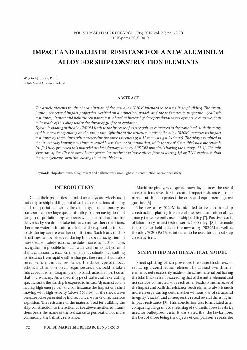
POLISH MARITIME RESEARCH, No 1/201572
POLISH MARITIME RESEARCH 1(85) 2015 Vol. 22; pp. 72-7810.1515/pomr-2015-0010
IMPACT AND BALLISTIC RESISTANCE OF A NEW ALUMINIUM ALLOY FOR SHIP CONSTRUCTION ELEMENTS
Wojciech Jurczak, Ph. D.Polish Naval Academy, Poland
ABSTRACT
The article presents results of examination of the new alloy 7020M intended to be used in shipbuilding. The exam-ination concerned impact properties, verified on a numerical model, and the resistance to perforation (ballistic resistance). Impact and ballistic resistance tests aimed at increasing the operational safety of marine construc-tions to be made of this alloy under the threat of gunfire or explosion. Dynamic loading of the alloy 7020M leads to the increase of its strength, as compared to the static load, with the range of this increase depending on the strain rate. Splitting of the structure made of the alloy 7020M increases its impact resistance by three times when preserving the same thickness (g = 12 mm <=> g = 2x6 mm). The alloy examined in the structurally homogenous form revealed low resistance to perforation, while the use of 6 mm thick ballistic ceramic (Al2O3) fully protected this material against damage done by ŁPS 7,62 mm shells having the energy of 3 kJ. The split structure of the alloy ensured better protection against explosive pieces formed during 1,4 kg TNT explosion than the homogeneous structure having the same thickness.
Keywords: ship aluminium alloy, impact and ballistic resistance, light ship construction, operational safety
INTRODUCTION
Due to their properties, aluminium alloys are widely used not only in shipbuilding, but al-so in constructions of many land transportation means. The economy of contemporary sea transport requires large speeds of both passenger navigation and cargo transportation. Agree-ments which define deadlines for deliveries by sea do not take into account weather conditions, therefore watercraft units are frequently exposed to impact loads during severe weather condi-tions. Such loads of ship structures can be observed during high-speed navigation on heavy sea. For safety reasons, the state of sea equal to 3˚ B makes navigation impossible for such watercraft units as hydrofoil ships, catamarans, etc., but in emergency situations, resulting for instance from rapid weather changes, these units should also reveal sufficient impact resistance. The above type of impact actions and their possible consequences are, and should be, taken into account when designing a ship construction, in particular that of a warship. As a special type of watercraft exe-cuting specific tasks, the warship is exposed to impact (dynamic) action having high energy den-sity, for instance the impact of a shell moving with high velocity (above 500 m/s), or the shock wave pressure pulse generated by indirect underwater or direct surface explosion. The resistance of the material used for building the ship construction to the action of the abovementioned muni-tions bears the name of the resistance to perforation, or more commonly: the ballistic resistance.
Maritime piracy, widespread nowadays, forces the use of constructions revealing in-creased impact resistance also for merchant ships to protect the crew and equipment against gun-fire [6].
The new alloy 7020M is intended to be used for ship construction plating. It is one of the best aluminium alloys among those presently used in shipbuilding [7]. Positive results of laborato-ry impact tests of series 7000 alloys [8] have made the basis for field tests of the new alloy 7020M as well as the alloy 7020 (PA47tb), intended to be used for combat ship constructions.
SIMPLIFIED MATHEMATICAL MODEL
Sheet splitting which preserves the same thickness, or replacing a construction element by at least two thinner elements, not necessarily made of the same material but having the total thickness not exceeding that of the initial element and not surface-connected with each other, leads to the increase of the impact and ballistic resistance. Such elements absorb much more en-ergy during deformation without loss of structural integrity (cracks), and consequently reveal several times higher impact resistance [9]. This conclusion was formulated after comparing dia-grams of stretching of synthetic fibres in fabrics used for bulletproof vests. It was stated that the kevlar fibre, the best of those being the objects of comparison, reveals the
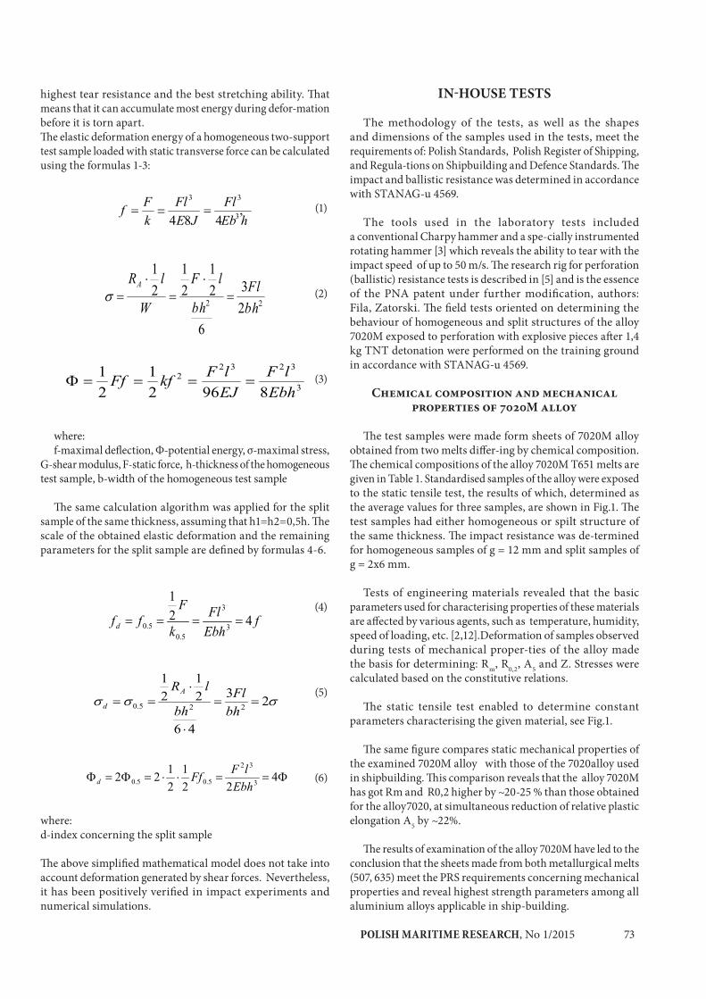
POLISH MARITIME RESEARCH, No 1/2015 73
highest tear resistance and the best stretching ability. That means that it can accumulate most energy during defor-mation before it is torn apart.The elastic deformation energy of a homogeneous two-support test sample loaded with static transverse force can be calculated using the formulas 1-3:
(1)
(2)
(3)
where: f-maximal deflection, Φ-potential energy, σ-maximal stress,
G-shear modulus, F-static force, h-thickness of the homogeneous test sample, b-width of the homogeneous test sample
The same calculation algorithm was applied for the split sample of the same thickness, assuming that h1=h2=0,5h. The scale of the obtained elastic deformation and the remaining parameters for the split sample are defined by formulas 4-6.
(4)
(5)
(6)
where: d-index concerning the split sample
The above simplified mathematical model does not take into account deformation generated by shear forces. Nevertheless, it has been positively verified in impact experiments and numerical simulations.
IN-HOUSE TESTS
The methodology of the tests, as well as the shapes and dimensions of the samples used in the tests, meet the requirements of: Polish Standards, Polish Register of Shipping, and Regula-tions on Shipbuilding and Defence Standards. The impact and ballistic resistance was determined in accordance with STANAG-u 4569.
The tools used in the laboratory tests included a conventional Charpy hammer and a spe-cially instrumented rotating hammer [3] which reveals the ability to tear with the impact speed of up to 50 m/s. The research rig for perforation (ballistic) resistance tests is described in [5] and is the essence of the PNA patent under further modification, authors: Fila, Zatorski. The field tests oriented on determining the behaviour of homogeneous and split structures of the alloy 7020M exposed to perforation with explosive pieces after 1,4 kg TNT detonation were performed on the training ground in accordance with STANAG-u 4569.
Chemical composition and mechanical properties of 7020M alloy
The test samples were made form sheets of 7020M alloy obtained from two melts differ-ing by chemical composition. The chemical compositions of the alloy 7020M T651 melts are given in Table 1. Standardised samples of the alloy were exposed to the static tensile test, the results of which, determined as the average values for three samples, are shown in Fig.1. The test samples had either homogeneous or spilt structure of the same thickness. The impact resistance was de-termined for homogeneous samples of g = 12 mm and split samples of g = 2x6 mm.
Tests of engineering materials revealed that the basic parameters used for characterising properties of these materials are affected by various agents, such as temperature, humidity, speed of loading, etc. [2,12].Deformation of samples observed during tests of mechanical proper-ties of the alloy made the basis for determining: Rm, R0,2, A5 and Z. Stresses were calculated based on the constitutive relations.
The static tensile test enabled to determine constant parameters characterising the given material, see Fig.1.
The same figure compares static mechanical properties of the examined 7020M alloy with those of the 7020alloy used in shipbuilding. This comparison reveals that the alloy 7020M has got Rm and R0,2 higher by ~20-25 % than those obtained for the alloy7020, at simultaneous reduction of relative plastic elongation A5 by ~22%.
The results of examination of the alloy 7020M have led to the conclusion that the sheets made from both metallurgical melts (507, 635) meet the PRS requirements concerning mechanical properties and reveal highest strength parameters among all aluminium alloys applicable in ship-building.
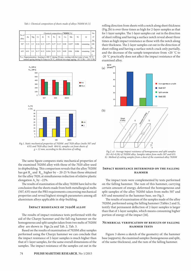
POLISH MARITIME RESEARCH, No 1/201574
Tab.1. Chemical composition of sheets made of alloys 7020M tb [1]
0
100
200
300
400
500
600
507 635 484/4
Rm [MPa]R0,2 [MPa]
Rm
R0,2
0
5
10
15
20
25
30
35
40
45
507 635 484/4
A5 [%]
Z [%]
A5
Z
Fig.1. Static mechanical properties of 7020M and 7020 alloys (melts 507 and 635) and 7020 alloy (melt 484/4), samples cut from sheets of
g = 12 mm, according to the direction of rolling
The same figure compares static mechanical properties of the examined 7020M alloy with those of the 7020 alloy used in shipbuilding. This comparison reveals that the alloy 7020M has got Rm and R0,2 higher by ~ 20-25 % than those obtained for the alloy 7020, at simultaneous reduction of relative plastic elongation A5 by ~22%.
The results of examination of the alloy 7020M have led to the conclusion that the sheets made from both metallurgical melts (507, 635) meet the PRS requirements concerning mechanical properties and reveal highest strength parameters among all aluminium alloys applicable in ship-building.
Impact resistance of 7020M alloy
The results of impact resistance tests performed with the aid of the Charpy hammer and the fall-ing hammer on the homogeneous and split samples taken from two melts of 7020M alloy are shown in Figs.2a and Tab. 2, Tab. 3.
Based on the results of examination of 7020M alloy samples performed using the Charpy hammer we can conclude that the impact resistance of 2-layer samples is much higher than that of 1-layer samples, for the same overall dimensions of the samples. The impact resistance of the samples cut out in the
rolling direction from sheets with a notch along sheet thickness (Fig.2b) is over three times as high for 2-layer samples as that for 1-layer samples. The 1-layer samples cut out in the direction of sheet rolling and having a surface notch reveal about three times as high impact resistance as those with the notch along their thickness. The 2-layer samples cut out in the direction of sheet rolling and having a surface notch crack only partially, and the decrease of the sample temperature from +20 ˚C to -20 ˚C practically does not affect the impact resistance of the examined alloy.
Impact resistance determined on the falling hammer
The impact tests were complemented by tests performed on the falling hammer. The ram of this hammer, carrying certain amount of energy, deformed the homogeneous and split samples of the alloy 7020M taken from melts 507 and 635 and mounted in the hammer base, see Fig.3.
The results of examination of the samples made of the alloy 7020M, performed using the falling hammer (Tables 2 and 3), testify that permanent deflection of 2-layer samples is larger than that of 1-layer samples, which means consuming higher portion of energy of the impact [16].
Numerical verification of results of falling hammer tests
Figure 3 shows a sketch of the geometry of: the hammer base (supports), the examined samples (homogeneous and split, of the same thickness), and the ram of the falling hammer.
0
10
20
30
40
50
60KCV [J/cm2]
geneous le
Melt 507
Melt 635
Fig.2. a)- Average impact resistance of homogeneous and split samples (h1=h2=0,5h) of 7020M alloy. Samples taken from melts 507 and 635.
b)- Method of cutting samples from a sheet of the examined alloy 7020M
(a)
(b)
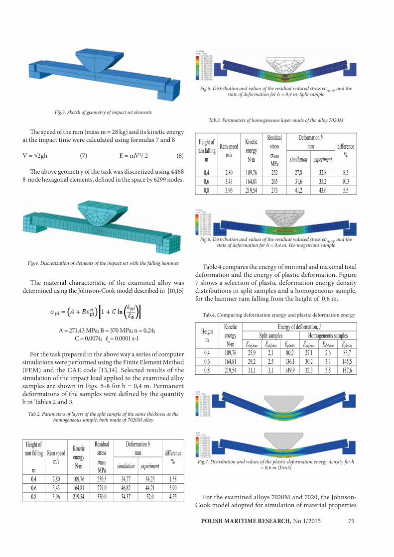
POLISH MARITIME RESEARCH, No 1/2015 75
Fig.3. Sketch of geometry of impact set elements
The speed of the ram (mass m = 28 kg) and its kinetic energy at the impact time were calculated using formulas 7 and 8
V = √2gh (7) E = mV2/ 2 (8)
The above geometry of the task was discretized using 4468 8-node hexagonal elements, defined in the space by 6299 nodes.
Fig.4. Discretization of elements of the impact set with the falling hammer
The material characteristic of the examined alloy was determined using the Johnson-Cook model described in [10,15]
A = 271,43 MPa; B = 370 MPa; n = 0,24; C = 0,0074; ἐo= 0.0001 s-1
For the task prepared in the above way a series of computer simulations were performed using the Finite Element Method (FEM) and the CAE code [13,14]. Selected results of the simulation of the impact load applied to the examined alloy samples are shown in Figs. 5-8 for h = 0,4 m. Permanent deformations of the samples were defined by the quantity b in Tables 2 and 3.
Fig.5. Distribution and values of the residual reduced stress eσHMH, and the state of deformation for h = 0,4 m. Split sample
Tab.2. Parameters of layers of the split sample of the same thickness as the homogeneous sample, both made of 7020M alloy
Tab.3. Parameters of homogeneous layer made of the alloy 7020M
Fig.6. Distribution and values of the residual reduced stress eσHMH, and the state of deformation for h = 0,4 m. Ho-mogeneous sample
Table 4 compares the energy of minimal and maximal total deformation and the energy of plastic deformation. Figure 7 shows a selection of plastic deformation energy density distributions in split samples and a homogeneous sample, for the hammer ram falling from the height of 0,6 m.
Tab.4. Comparing deformation energy and plastic deformation energy
Fig.7. Distribution and values of the plastic deformation energy density for h = 0,6 m (J/m3)
For the examined alloys 7020M and 7020, the Johnson-Cook model adopted for simulation of material properties

POLISH MARITIME RESEARCH, No 1/201576
was taken from [13,14] with the following data: density ρ = 2700 kg / m3; Young’s modulus – E = 9,1.104 MPa; Poisson’s ratio – ν = 0,34; yield strength – Re= 271,43 MPa; strength limit – Rm= 400 MPa.
Strain rate related dynamic properties of 7020M alloy
The increased strain rate leads to the increase of plastic deformation resistance of metals, with the increase of the yield point, strength limit, and hardness limit as further consequences [4].
The information on impact mechanical properties of the material is needed when evaluating the real impact resistance of the watercraft construction [11]. The strain rate tests were performed for the speed of impact equal to: 10, 20 and 30 [m/s]. In Table 5,0 [m/s] denotes static properties at the impact speed V≤ 0-2 m/s. Detailed results of the examination oriented on determining the effect of strain rate on mechanical properties are collected in Table 5.
Ballistic resistance of 7020M alloy
Tests of resistance to perforation (ballistic resistance) were performed by firing a 7,62 mm ŁPS shell with steel core to homogeneous and split samples (ϕ 50 mm) of the alloy 7020M from a distance of 1,5-2 mm, while the tests of ballistic (explosive) resistance of homogeneous plates of 12 mm in thickness and split plates 2x6 mm, both made of 7020M alloy, were performed by ex-posing the plates to detonation of a high explosive grenade, type OF412, calibre 100 mm, filled with 1,4 kg TNT, taking place at a distance of 0,6 m according to STANAG-u 4569.
Fig.8a. Effects of firing the ŁPS shell with steel core and the energy of 3 kJ to 7020M alloy from the dis-tance of 2 m - unprotected sample
Fig.8b. Effects of firing the ŁPS shell with steel core and the energy of 3 kJ to 7020M alloy from the dis-tance of 2 m - sample protected with ceramic
Al2O3 of g = 6 mm
The effects of the action of the air shock wave pressure pulse on the examined homogeneous and split sheets of 7020M alloy are shown in Fig.9.
Compared to the homogeneous plate, the split plates (g = 2 x 6 mm) made of 7020M alloy re-vealed better capability of minimising the effects of detonation of high explosive charge, thus increasing the safety of navigation in situations threatening with explosion. The perforation of the homogeneous plate seen in Fig.9a reveals that the detonation pieces punch the plate and may pose a threat. In contrary to that, the inner plate shown in Fig.5bw captures part of the pieces while the outer plate, shown in Fig. 9bz, either captures the pieces or entirely cracks (without defragmentation). Such favourable results are not observed in tests checking the resistance to perforation. The examined alloy 7020M, even split in the same thickness, does not protects against the ŁPS shell of calibre 7,62 and energy 3 kJ which generates pieces during perforation, see Fig.8a. However, total protection in this case can be ensured by an additional layer of ballis-tic ceramic (Al2O3) of g = 6 mm, as shown in Fig.8b.

POLISH MARITIME RESEARCH, No 1/2015 77
Tab.5. Collation of average dynamic mechanical properties of samples made of 7020M alloy, melts 507 and 635, exposed to different strain rates
Fig.9. Effects of 7020M alloy sheet perforation (dimensions 300x3000): a) homogeneous g = 12 mm b) split (w-inner, z –outer from the source of explosion, total thickness g = 2x6 mm) after detonation of high explosive shell of OF412 type and calibre 100 mm with the contents of 1,4 kg of TNT, taking place at
a distance of 0,6 m.
FINAL CONCLUSIONS
The performed tests of samples made of 7020M alloy allow the following conclu-sions to be formulated:
1.The increase of dynamic load has led to the increase of strength parameters of the ex-amined alloy 7020M, as compared to the values obtained in the static tensile test.
2.Strenght and plastic properties of the examined aluminium alloy depend on the strain rate and the load energy density.
3. Conclusions resulting from tests performed with the Charpy hammer
a. Impact resistance of the samples split along the thickness is over three times as high as that of the samples with homogeneous structure along the thickness.
b. Impact resistance of the samples having homogeneous structure along the surface in approximately three time as high as that of the homogeneous samples along the thick-ness.
c. During the Charpy hammer tests, the samples split along the surface did not crack entirely, while the homogeneous samples along the thickness totally cracked
d. The applied adhesive does not affect the impact resistance of the split samples.
4. Permanent deflection of the split samples being the result of the falling hammer action is much larger than that of the homogeneous samples.
The alloy 7020M is a highly resistant alloy, with Rm =
= 400-500 MPa, and simultaneous-ly preserves good plastic properties. Its high resistance to corrosion in sea environment [2], along with neutral reaction to magnetic forces and weldability, make this alloy ap-plicable for constructions of marine transportation means. However, the following recommendations related to terrorist threat safety are to be taken into account when using this alloy:
- important ship compartments made of 7020M alloy should be additionally protected against bullets using ballistic ceramic of minimal thickness of 6 mm.
- marine constructions built using this alloy should have a split structure, provided that technological aspects make it possible.
REFERENCES
1. Attestation IMN-OML no. 4550/91,336 OML/91.
2. Cudny K, Powierża Z.: Selected issues of impact resistance of ships (in Polish). Script WSMW 1978.
3. Dobrociński St., Fila J, Jurczak W.,Kolenda J.: Impact and ballistic resistance of a new aluminium alloy and composites making use of it (in Polish). Statute work of AMW 1999-2001 pk. „BALIDUR”
POLISH MARITIME RESEARCH, No 1/201578
4. Fila J.: Examining the effect of the loading state and strain rate on the strength and duc-tility of shipbuilding materials (in Polish). Conference on “Impact resistance of struc-tures”, AMW, Gdynia 1993.
5. Fila J., Zatorski Z. et al.: Reports no 1/1993, 1/94, and 2/95 of IPBMO/”Shell” - AMW-KBN 1993-95.
6. Grządziela A., Jurczak W.: Current problem of sea transport safety. Logistyka 6/2014
7. Jurczak W.: The effect of chemical composition and heat treatment on mechanical properties and corrosion resistance of Al-Zn-Mg alloys intended to be used for welded ship constructions (in Polish) . Ph.D. thesis, PG 1998.
8. Jurczak W. Kyzioł L.: Dynamic properties of 7000-series aluminium alloys at large strain rates. Polish Maritime Research 1 (72) vol.19 2012
9. Jurczak W. Kolenda J.: Patent submission – three-layer shield (in Polish), 2004
10. Jurczak W., Szturomski B., Simulating the Impact of Exposure to Corrosive Medium on Cracking Initiation in AW7020M Alloy Specimens, Solid State Phenomena, Trans Tech Periodicals published by Trans Tech Publications Ltd., Zurich, Switzerland 2014,
CONTACT WITH THE AUTHOR
Wojciech Jurczak
The Naval AcademyName of Heroes of the Westerplatte
69 Śmidowicza Str.81-103 Gdynia
POLAND
11. Kinslov R. at al.: High-Velocity Impact Phenomena. Academic Press, New York and London, 1970.
12. Levedahl W., Capable A.: Affordable 21st - Century Destroyer. Naval Engineers Journal. May 1993, pp. 213-223
13. Szturomski B.: Principles of the Finite Element Method (in Polish), Wydawnictwo Akademickie Akademii Marynarki Wojennej w Gdyni, Gdynia 2011
14. Szturomski B.: Engineering applications of FEM for solving solid body problems, as illustrated by the code ABAQUS (in Polish), Wydawnictwo Akademickie Akademii Marynarki Wojennej w Gdyni 2013
15. Szturomski B., Jurczak W.: Operating wear of ship aluminium alloys 7020 and 7020M (in Polish), Energetyka, Wortal Branżowy, no. 8 (698) 2012,
16. Wiśniewski A.: Armours – structure, designing and testing (in Polish). WNT, War-saw 2001