Embed Size (px)
Citation preview

NMR Spectroscopy: Principles and Applications
Nagarajan Murali
2D NMR – Homonuclear 2D
Lecture 6

2D-NMRTwo dimensional NMR is a novel and non-trivial
extension of 1D NMR spectroscopy. In the simplest form of understanding the (a) 1D spectrum is a plot of intensity vs frequency, whereas the (b) 2D NMR spectrum is a plot of intensity vs two independent frequency axes.

NMR Signal in Two-Time PeriodsWe know that NMR signals are detected as a
function of time and 2D NMR thus implies we have NMR signal as a function of two independent time periods. Any 2D NMR scheme can be represented in general as below.
NMR Signal in Two-Time PeriodsIn the preparation period equilibrium
magnetization is built-up and transformed into coherences that evolve during the evolution (t1) period. The evolution period is incremented systematically in successive experiments. During the mixing period a coherence /magnetization transfer is effected which then get detected during the detection period.

NMR Signal in Two-Time PeriodsThe systematic incrementation of the t1 interval
and direct detection of NMR signal during t2
gives two dimensional time domain data.
2
1
) (
1*
) (
1
2
1
widthspctralNt
widthspctral

NMR Signal in Two-Time Periods
The time domain signal S(t1,t2) up on two dimensional Fourier transform yields two dimensional spectrum S(1, 2).

Correlated Spectroscopy (COSY)Let us now focus on the very basic 2D NMR experiment called COSY.
We analyzed a special case in the 1D section as a selective correlation experiment. Here, we analyze the 2D version that gives correlation between all J coupled protons. The pulse sequence is give an as follows:
The experiment is repeated N – times with systematic incrementation of the t1 time and the data collected is subjected to double FT to yield 2D spectrum.

Correlated Spectroscopy (COSY)
A typical COSY spectrum will have two types of peaks –diagonal peaks that correlate the shifts of the same spins in both 1 and 2 dimensions, and cross peaks that correlate spin A with spin B by the process of coherence transfer by the second pulse in the sequence.

HamiltonianTwo Spins I=1/2 and J Coupling
Let us again use the two spin Hamiltonian in which each spin with spin I=1/2 and J Coupling between them.
In subsequent discussions we will drop the hat from the operators and represent them as normal face italic character for convenience.
1202012112202101 case for the Hzin JJ zzzz IIIIH
s rad and frame rotatingin 2 1-21122211 zzzz IIIIH
J
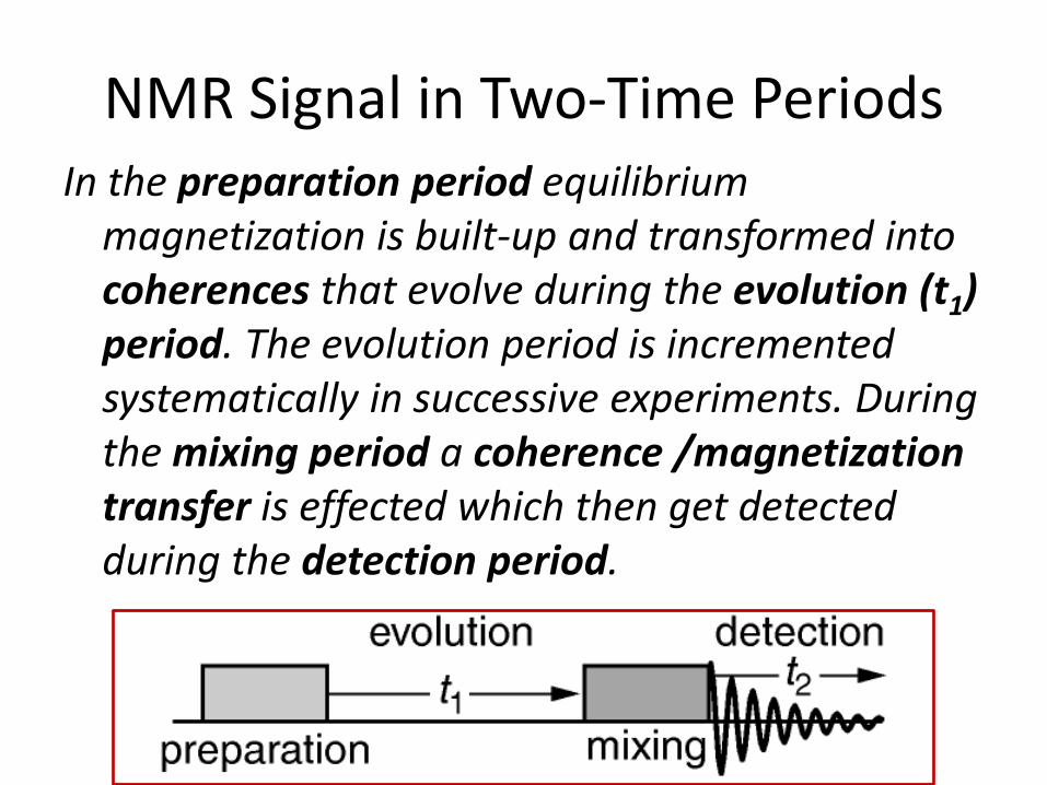
COSY ExperimentLet us consider two protons coupled to each other and we apply
the COSY pulse sequence that has two non selective 90o x-pulses. Let us just follow spin 1 and by induction we can write for spin 2.
yzx
yxz
I
zyx
zxy
IItJxy
Ity
I
z
IItJtItJt
IItJtItJt
IItJtItJt
IItJtItJt
tItIII
x
zzzx
2111211111211
2111211111211
2
2111211111211
2111211111211
21111111
21
2)sin()sin()cos()sin(
2)sin()cos()cos()cos(
2)sin()sin()cos()sin(
2)sin()cos()cos()cos(
)sin()cos( 21112111
Detectable terms

COSY ExperimentFocusing just on the detectable terms, we have the signal at the
start of t2 as
The I1x term will give a doublet at frequency 1 in the 2
dimension and is modulated in t1 by sin(1 t1) giving rise to the diagonal peak.
The term 2I1zI2y will give an anti-phase doublet at frequency 2 in the 2 dimension and is modulated in t1 by sin(1 t1) giving rise to the cross peak.
In the 1 dimension the doublet structure of the diagonal peak is in-phase (cosine function), whereas that of the cross peak is anti-phase (sine function).
yzx IItJtItJt 2111211111211 2)sin()sin()cos()sin(

COSY ExperimentFocusing just on the detectable terms, we have the signal at the
start of t2 as
yzx IItJtItJt 2111211111211 2)sin()sin()cos()sin(
1
21
1
2
2

COSY ExperimentLet us analyze the cross peak multiplet structure.
yzx IItJtItJt 2111211111211 2)sin()sin()cos()sin(
))cos()(cos(2
1)sin()sin( 1121112111211 tJtJtJt
cross peak structureyz II 212
1121
1121
)cos(
)cos(
tJ
tJ

COSY ExperimentLet us analyze the diagonal peak multiplet structure.
yzx IItJtItJt 2111211111211 2)sin()sin()cos()sin(
))sin()(sin(2
1)cos()sin( 1121112111211 tJtJtJt
diagonal peak structurexI1
1121
1121
)sin(
)sin(
tJ
tJ

112
112
)cos(
)cos(
tJ
tJ
I
I
COSY ExperimentThe cross peaks and diagonal peaks will have different phases as
they are 900 out of phase in both 1 and 2 dimension.
diagonal peak structure
xI1
112
112
)sin(
)sin(
tJ
tJ
I
I
yz II 212
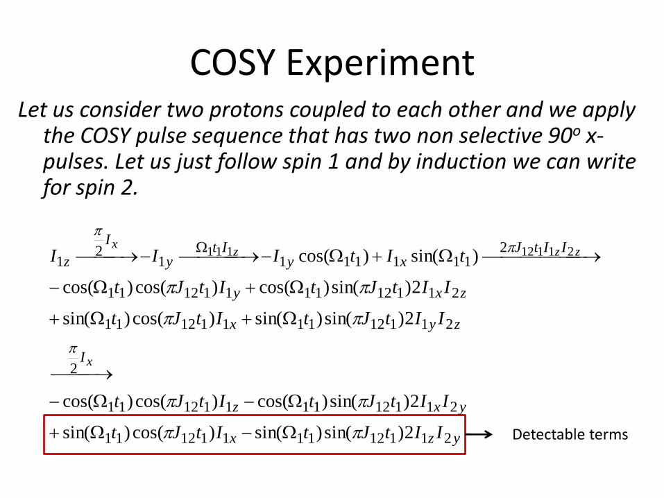
COSY ExperimentThe diagonal peak will be dispersive mode in both dimension and
the cross peak will be in absorptive mode .
2D absorption mode lineshape
2D dispersion mode lineshape

COSY ExperimentThe anti-phase structure of the cross peaks is a problem because,
if the line width exceeds the J coupling then the anti-phase doublet overlap and the peak vanishes. Whereas, the diagonal peaks have in-phase multiplets and add in signal strength in overlap situations exacerbating the problem. (a) Simulation shows the effect of overlap and in (b) a real situation with added noise is shown. The line width is about 1/5 of J value on the left most spectrum.
In (a) the smallest coupling constant (Jmax/64) is still visible, but in (b) due to noise even (Jmax/32) is barly visible. Thus the ability to see a cross peak for small coupling depends on linewidth and noise.

COSY ExperimentThe COSY spectrum below illustrate the usefulness of the
experiment in identifying the spin system in a molecule.
Azo-sugar

COSY ExperimentThe COSY spectrum below illustrate the usefulness of the
experiment in identifying the spin system in a molecule.
Carbopeptoid

2D FT
We have seen in detail 1D FT in Lecture 3. We summarize the result here as
Where A() is the absorption mode lineshapeand D() is the dispersion mode line shape. Furthermore, we can also do cosine and sine FT.
)()()exp()exp( 00 iDASRttiSFT
)()exp()sin(
)()exp()sin(
)()exp()cos(
)()exp()cos(
0sin
0
0cos
0
0sin
0
0cos
0
ASRttS
DSRttS
DSRttS
ASRttS
FT
FT
FT
FTin

NMR Signal in Two-Time Periods
(a) Time domain signal (cosine modulated in t1
and t2). (b) cos-FT with respect to t2 and (c) cos-FT with respect to t1.
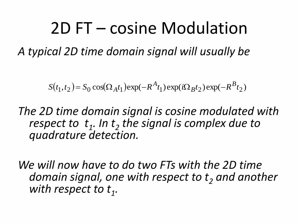
2D FT – cosine ModulationA typical 2D time domain signal will usually be
The 2D time domain signal is cosine modulated with respect to t1. In t2 the signal is complex due to quadrature detection.
We will now have to do two FTs with the 2D time domain signal, one with respect to t2 and another with respect to t1.
)exp()exp()exp(cos, 2211021 tRtitRtSttS BB
AA

2D FT – cosine ModulationFT with respect to t2 yields,
Then 2D we do a cosine FT with respect to t1.
where A1(A) is the absorption mode lineshape along 1 axis. The real part of the above expression gives a 2D spectrum with absorption lineshape in both frequency axes.
)()()exp(cos),(, 211021212
BBA
AtFT
iDAtRtStsttS
)()()()(,
)()()(),(,
21210cos
21
221021cos
21
2
2
BABAtFT
BBAtFT
DiAAAStS
iDAASstS

2D FT
The 2D spectrum of the expression below is a double absorption lineshape 2D peak.
)()(,Re 21021 BA AASS

2D FT – sine ModulationSometime, we can also have a sine modulated t1 signal as
The FT along t2 gives then,
Then we do a sine FT with respect to t1.
where A1(A) is the absorption mode lineshape along 1 axis. The real part of the above expression gives, as before, a 2D spectrum with absorption lineshape in both frequency axes.
)()()exp(sin),(, 211021212
BBA
AtFT
iDAtRtStsttS
)()()()(,
)()()(),(,
21210sin
21
221021sin
21
2
2
BABAtFT
BBAtFT
DiAAAStS
iDAASstS
)exp()exp()exp(sin, 2211021 tRtitRtSttS BB
AA

2D FT – cosine/sine Modulation
The disadvantage of having just a cosine or sine modulation in t1 is that there is no frequency sign discrimination. We can see this from the properties of FT.
)()exp()sin(
)()exp()sin(
)()exp()cos(
)()exp()cos(
)()()exp()exp(
0sin
0
0cos
0
0sin
0
0cos
0
00
ASRttS
DSRttS
DSRttS
ASRttS
iDASRttiS
FT
FT
FT
FTin
FTcomplex
)sin()sin(
)cos()cos(
tt
tt

2D FT – cosine + sine Modulation
We can, however, generate 2D signals that is both sine and cosine modulated in t1,
It is useful to collect both signals, usually in two experiments, so that frequency sign discrimination can be achieved in the t1 time domain.
)exp()exp()exp(sin, 2211021 tRtitRtSttS BB
AAs
)exp()exp()exp(cos, 2211021 tRtitRtSttS BB
AAc

2D FT – cosine + sine Modulation
A complex modulation in t1 can be generatedas P-type signal and N-type signal
The resulting spectrum from these complex signals will be frequency discriminated.
)exp()exp()exp(exp
)exp()exp()exp(sin)cos(,
,,),(
22110
22111021
212121
tRtitRtiS
tRtitRtitSttS
ttiSttSttS
BB
AA
BB
AAAP
scP
)exp()exp()exp(exp
)exp()exp()exp(sin)cos(,
,,),(
22110
22111021
212121
tRtitRtiS
tRtitRtitSttS
ttiSttSttS
BB
AA
BB
AAAN
scN

2D FT P-type Modulation
2D FT of the complex signal is written as,
A complex FT along t1 yields a spectrum
A plot of either the real part or the imaginary part will yield a phase twisted lineshape.
)]()()[exp(exp),( 2211021 BBA
AP iDAtRtiStS
)]()()()([)]()()()([
)]()()][()([),(
21212121
221121
BABABABA
BBAAP
ADDAiDDAA
iDAiDAS
Real Part Imaginary Part

2D FT P-type Modulation
A typical phase twisted lineshape is shown below.
Such a lineshape is undesirable in high resolution work.

2D FT N-type Modulation
2D FT of the complex signal is written as,
A complex FT along t1 yields a spectrum
A plot of either the real part or the imaginary part will yield a phase twisted lineshape.
)]()()[exp(exp),( 2211021 BBA
AN iDAtRtiStS
)]()()()([)]()()()([
)]()()][()([),(
21212121
221121
BABABABA
BBAAN
ADDAiDDAA
iDAiDAS
Real Part Imaginary Part

2D Hyper Complex DataWe can use the cosine and sine modulated data to form a hyper complex 2D data
that will yield a pure absorption spectrum data. Start with cosine modulated signal and do a FT along t2
We then take the real part of the signal
We do the same process for the sine modulated signal.
Now we form a new complex signal from these two signals,
)()()exp(cos),( 211021 BBA
Ac iDAtRtStS
)()exp(cos),( 211021, BA
ARc AtRtStS
)()exp(sin),( 211021, BA
ARs AtRtStS
)()exp()exp(
)()exp(]sin[cos
),(),(),(
2110
21110
21,21,21
BA
A
BA
AA
RsRc
AtRtiS
AtRtitS
tiStStS

2D Hyper Complex Data
The usual complex FT along t1will then yield the desired spectrum.
We then take the real part of the 2D FT to get double absorption lineshape with frequency discrimination. This method of data collection and Fourier transform is known as States-Haberkorn-Ruben method or simply States method.
)()()()(),(
)()]()([),(
)()exp()exp(),(
212121
21121
211021
BABA
BAA
BA
A
AiDAAS
AiDAS
AtRtiStS

Time Proportional Phase Incrementation (TPPI)
We need complex data along t1 to discriminate positive frequency from negative frequency. But by some means if we can set all frequencies to be positive then we don not need complex signal.
One way to achieve this is to set the reference frequency at the end of the spectrum and leave the negative frequency region empty. But this wastes data space. In TPPI, we leave the reference frequency at the center but move the offsets to look like all the frequencies are positive.

Time Proportional Phase Incrementation (TPPI)
Let us start with the cosine and sine modulated signals:
We know sine and cosine functions differ only in phase, a shift of one quarter period or a phase of /2 radians converts one to the other.
)exp()exp()exp(sin,
)exp()exp()exp(cos,
2211021
2211021
tRtitRtSttS
tRtitRtSttS
BB
AAs
BB
AAc
2for sin
sinsincoscos)cos(
t
ttt

Time Proportional Phase Incrementation (TPPI)
We can then simply add a phase to the cosine modulated function that is defined as
If we set the phase =(2fmax)*t1 then we can shift all the frequencies will be shifted to the right.
)exp()exp()exp(][cos
)exp()exp()exp(cos,,
22110
22111021
tRtitRtS
tRtitRttSttS
BB
AaddA
BB
AaddA
1tadd

States –TPPI MethodBoth States and TPPI
methods have advantages and thus combining them in a 2D experiments is ideal. A COSY experiment with States-TPPI method can be represented as below.
2
11
) (
1*
) *2(
1
2
'
widthspctralNt
widthspctral

COSY Experiment2D-FT of FID from such an experiment yields a spectrum with the diagonal
peak in dispersive mode in both dimension and the cross peak in absorptive mode.
2D absorption mode lineshape
2D dispersion mode lineshape

Double Quantum Filtered COSY (DQFC)
The disadvantages of COSY can be alleviated by double quantum filtered COSY experiment in which the diagonal multiplets are also anti-phase like the cross peaks and in same phase. This leads to better resolution near diagonal and cleaner looking spectrum. The pulse sequence is shown below.
DQFC
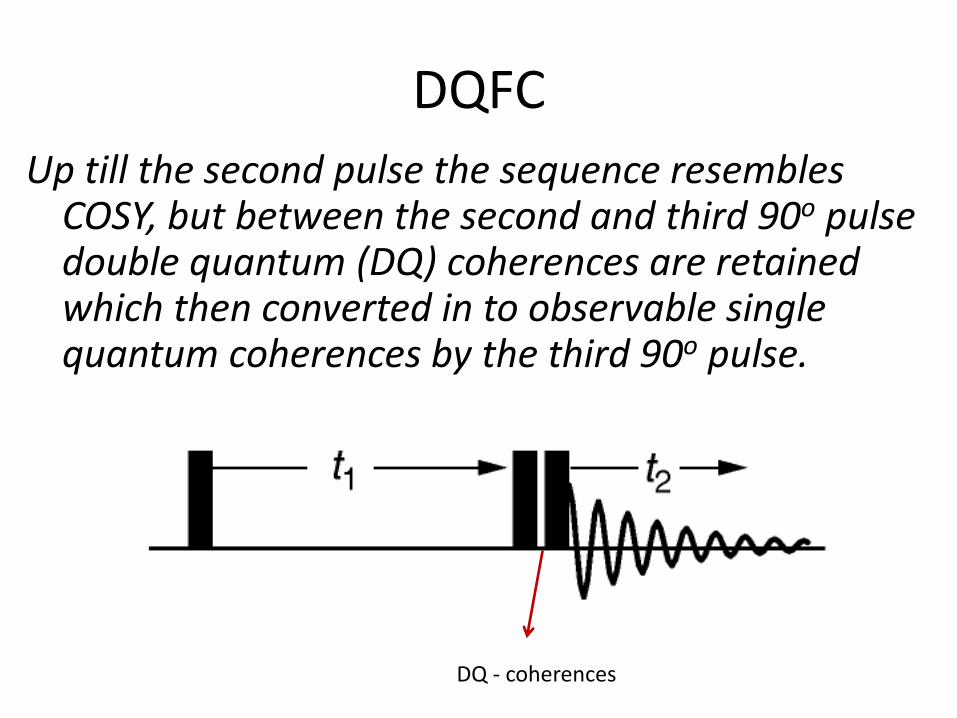
Up till the second pulse the sequence resembles COSY, but between the second and third 90o pulse double quantum (DQ) coherences are retained which then converted in to observable single quantum coherences by the third 90o pulse.
DQ - coherences

DQFC
If we follow the evolution of spin 1, from the analysis of COSY we have right after the second 90o pulse
Only the term highlighted is retained and is sum of double quantum and zero quantum term.
yzx
yxz
IItJtItJt
IItJtItJt
2111211111211
2111211111211
2)sin()sin()cos()sin(
2)sin()cos()cos()cos(

DQFC
After the second 90o pulse we retaiin only the DQC.
)22(2
1)sin()cos(
2
22()22(2
1)sin()cos(
2)sin()cos(
212111211
2121212111211
2111211
xzzx
x
xyyxxyyx
yx
IIIItJt
I
IIIIIIIItJt
IItJt
DQ ZQ
Third 90o pulse

DQFC
The first term yields the diagonal peaks and the second term yields the cross peaks.
Also, both the diagonal and cross peaks are anti-phase multiplets in both 1 and 2 dimensions and have same phase characteristics in both dimensions.
)22(2
1)sin()cos( 212111211 xzzx IIIItJt
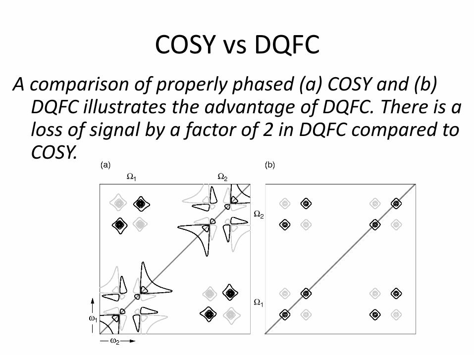
COSY vs DQFC
A comparison of properly phased (a) COSY and (b) DQFC illustrates the advantage of DQFC. There is a loss of signal by a factor of 2 in DQFC compared to COSY.

COSY vs DQFC
A region of DQFC of andrographolide illustrates the advantage of DQFC. Cross peaks close to diagonals can be seen better.

Total Correlation Spectroscopy (TOCSY)
COSY and DQFC connect, via cross peaks, spins that have coupling between them which can either be short range or long range. In a spin network let’s say spin A is coupled spin B but not to spin C and spin B is coupled spin C (i.e. JAC=0, JAB 0, JBC 0 ). Then in COSY or DQFC there will be a cross peak between spin A and spin B, spin B and spin C, but no cross peak between spin A and spin C. In a TOCSY experiment spin A to spin C cross peak will also appear and identify spins A, B, and C as a unique group of coupled spins.

Total Correlation Spectroscopy (TOCSY)
COSY TCOSY

Total Correlation Spectroscopy (TOCSY)
A typical TOCSY pulse sequence is given below.
The key part of the experiment is isotropic mixing caused by the spin locking field in the mixing period. Isotropic mixing converts I1z, I1x, and I1y to I2z, I2x, and I2y.

Total Correlation Spectroscopy (TOCSY)
Let us say we retain I1z at point A in the pulse sequence. The evolution of I1z during isotropic mixing yields at point B.
)22(2
1)2sin(
)2cos(12
1)2cos(1
2
1
212112
212112
1
yxxymix
zmixzmixmixingisotropic
z
IIIIJ
IJIJI

Total Correlation Spectroscopy (TOCSY)
If we just focus on the Iz terms, the last 90o pulse would rotate Iz to Iy which will produce in phase doublet in 2. The Iz term arose from the Iy in t1 period that had cosine modulations with respect to J coupling which will is also be an in-phase doublet.
Analytical solutions are not feasible for more than two spin system and the qualitative analysis does not show how a cross peak appear when the coupling is absent.
)2cos(12
1)2cos(1
2
1
2
)2cos(12
1)2cos(1
2
1
212112
212112
ymixymix
x
zmixzmix
IJIJ
I
IJIJ

Total Correlation Spectroscopy (TOCSY)
In a extended coupled network of spins I1z at point A in the pulse sequence transferred as to of I2z which then get transferred as I3z and so on during isotropic mixing. The transfer extends to more remote spins as the mixing time is increased.

Total Correlation Spectroscopy (TOCSY)
TOCSY of the azo-sugar. On the right the COSY is shown.