Embed Size (px)
Citation preview

7/28/2019 NMR Logging Principles and Applications
http://slidepdf.com/reader/full/nmr-logging-principles-and-applications 1/253
NMR LOGGINGPRINCIPLES & APPLICATIONS
G EORGE R. C OATES , L IZHI X IAO , AND M ANFRED G. P RAMMER

7/28/2019 NMR Logging Principles and Applications
http://slidepdf.com/reader/full/nmr-logging-principles-and-applications 2/253
i
NMR LoggingPrinciples and Applications

7/28/2019 NMR Logging Principles and Applications
http://slidepdf.com/reader/full/nmr-logging-principles-and-applications 3/253
iii
NMR LoggingPrinciples and Applications
George R. Coates, Lizhi Xiao, and Manfred G. Prammer
Halliburton Energy Services
Houston

7/28/2019 NMR Logging Principles and Applications
http://slidepdf.com/reader/full/nmr-logging-principles-and-applications 4/253
iv
Sales of Halliburton products and services will be in accord solely with the terms and conditions
contained in the contract between Halliburton and the customer that is applicable to the sale.
1999 Halliburton Energy Services. All rights reserved.
Printed in the United States of America
Halliburton Energy Services Publication H02308

7/28/2019 NMR Logging Principles and Applications
http://slidepdf.com/reader/full/nmr-logging-principles-and-applications 5/253
Table of Contents v
Halliburton Energy Services
Foreword xi
Preface xiii
Editors and Editorial Review Board xv
Acknowledgments xvii
Chapter 1 Summary of NMR Logging Applications and Benefits 1Medical MRI 1MRI Logging 2Comparison of the MRIL Tool to Other Logging Tools 2
Fluid Quantity 3
Fluid Properties 4Pore Size and Porosity 4
NMR-Logging Raw Data 6NMR Porosity 7NMR T
2Distribution 7
NMR Free-Fluid Index and Bulk Volume Irreducible 8NMR Permeability 9NMR Properties of Reservoir Fluids 11NMR Hydrocarbon Typing 11NMR Enhanced Water Saturation with Resistivity Data 16MRIL Application Examples 16
MRIL Porosity and Permeability 16
Low-Resistivity Reservoir Evaluation 22
MRIL Acquisition Data Sets 25MRIL Response in Rugose Holes 26NMR Logging Applications Summary 26References 28
Chapter 2 NMR Physics 33Nuclear Magnetism 33Polarization 34Pulse Tipping and Free Induction Decay 37Spin-Echo Detection 39
Contents
7/28/2019 NMR Logging Principles and Applications
http://slidepdf.com/reader/full/nmr-logging-principles-and-applications 6/253
NMR Logging Principles and Applications
vi Table of Contents
NMR-Measurement Timing 42References 43
Chapter 3 Fundamentals of NMR Petrophysics 45NMR Relaxation Mechanisms of Fluids in Rock Pores 45
Bulk Relaxation 47Surface Relaxation 48Diffusion-Induced Relaxation 48
Multi-Exponential Decay 51Echo-Fit for T
2Distribution 53
Pore Size Distribution 54Determination of BVI 57
Cutoff BVI 57
Spectral BVI 60
MRIL Permeability Model 64The Free Fluid Model 64The Mean T
2
Model 65
MRIL Porosity Model 65References 67
Chapter 4 Fundamentals of NMR Hydrocarbon Typing 77NMR Properties of Hydrocarbons 77NMR Hydrocarbon Typing 80
T 2
Distribution of a Partially Saturated Rock 80T
1Relaxation Contrast 80
Diffusivity Contrast 82Numerical Simulations 83
Oil Effects on T 2Distributions 84
Water and Light Oil 84
Water and Viscous Oil 85Effects of Viscosity and Wettability on the Oil Signal in a T 2
Distribution 85
Gas Effects on T 2
Distribution Under Different Conditions 87Water and Gas 88Water, Light Oil, and Gas 89
References 89
Chapter 5 MRIL Tool Principles 91Polarization 91Magnetization Tipping and Spin-Echo Detection 91Logging Speed and Vertical Resolution 94Depth of Investigation 96Multi-Frequency Measurement and RF Pulse Bandwidth 98
Ringing Effect 102Signal-to-Noise Ratio and Running Average 104Activations 104Tool Configuration 108References 108

7/28/2019 NMR Logging Principles and Applications
http://slidepdf.com/reader/full/nmr-logging-principles-and-applications 7/253
Table of Contents vii
Halliburton Energy Services
Chapter 6 Answer Products Derived from MRIL Stand-Alone Analysis 113Time Domain Analysis 113
Concept 113Principle 113
Differential Spectrum Method 113Time Domain Analysis 114
Data Acquisition 114Applications 116
Example 1 116
Example 2 116Example 3 116
Diffusion Analysis 122Concept 122Data Acquisition 123
Shifted Spectrum Method 124
Quantitative Diffusion Analysis: DIFAN 124Enhanced Diffusion Method 127
Appendix: TDA Mathematical Model 129
References 133
Chapter 7 Answer Products Derived fromMRIL Combinations with Other Logs 135
MRIAN Concept 135MRIAN Principles 135
Dual-Water Model 135Determining S
wbfor the Dual-Water Model 137
Quality Control on the Calculated S wb
137Determination of the W Exponent in MRIAN 138Calculation of S
wTin MRIAN 139
Parameters Affecting MRIAN Calculations 139
MRIL Data Acquisition for MRIAN 139MRIAN Applications 142
Low-Resistivity Reservoir 1 142Low-Resistivity Reservoir 2 142
Gas-Influx Monitoring with MRIL in an Arabian Gulf Carbonate 146Evaluation of a Shaly, Tuff Sandstone Formation Containing
Medium-Viscosity Oils 147MRIAN in a Light-Hydrocarbon Well 150
Well Completion with MRIL: StiMRIL 150References 154
Chapter 8 MRIL Job Planning 159Determining NMR Properties of Reservoir Fluids 160
Example 1: OBM, Gas 161Well Description 161Example 1, Step 1: Determine NMR Fluid Properties 161
Assessing the Expected Decay Spectrum of Reservoir Fluids in a Formation 162Example 1, Step 2a: Assess Expected NMR Response (T
2Distribution) 163
Assessing the Expected NMR Apparent Porosity of a Formation 164

7/28/2019 NMR Logging Principles and Applications
http://slidepdf.com/reader/full/nmr-logging-principles-and-applications 8/253
NMR Logging Principles and Applications
viii Table of Contents
Example 1, Step 2b: Assess Expected NMR Response (Apparent Porosity) 165
Selection of the Activation Set 166Standard T
2Activation 166
Dual-TW Activation 167
Dual-TE Activation 167Determination of the Activation Set and Acquisition Parameters 167
Standard T 2
Activations 168Example 1, Step 3: Determine Appropriate Activation Parameters (TW , TE , NE )
for a Standard T 2
Activation 168
Dual-TW Activations 169Example 1, Step 3: Determine Appropriate Activation Parameters (TW
L, TW
S, TE , NE )
for a Dual-TW Activation 170Example 2: OBM Dual TW 172Dual-TE Activations 174
Example 3: WBM, Viscous Oil, Dual TE 174Well Description 174
Step 1: Determine NMR Fluid Properties 175
Step 2: Assess Expected NMR Response 175Step 3: Determine Appropriate Activation Parameters (TE
L
, TE S
, TW , and NE )
for a Dual-TE Activation 175
Dual-TW /Dual-TE (Virgin Area Logging) 177Step 1: Determine NMR Fluid Properties 177
Step 2: Assess Expected NMR Response 177
Step 3: Determine Appropriate Activation Parameters(TW
L, TW
S, TE
L, TE
S, NE
L, and NE ) 177
Example 4: OBM, Gas, Dual TW , TE 178Well Description 178Step 1: Determine NMR Fluid Properties 178
Step 2: Assess Expected NMR Response 179Step 3: Determine Appropriate Activation Parameters (TW
i, TE
i, NE
i) 180
Other Considerations for MRIL Job Planning 181Formation Type (Sandstone, Carbonate, Chalk, Diatomite) 181Wettability 181
Mud Type (Oil-Based, Water-Based) 182Trade Off Logging Speed⇔ Accuracy (S / N , Sampling Rate) ⇔ Typeand Detail of Information 183
References 184
Chapter 9 MRIL Log Quality Control 185Concepts and Definitions 185
Gain and Q Level 185
B1
and B 1mod
186Chi 186
Noise Indicators: OFFSET, NOISE, RINGING, and IENoise 186Low-Voltage Sensors 187High-Voltage Sensors 187
Phase Correction Information: PHER , PHNO , and PHCO 188Temperature 189
Pre-Logging Calibration and Verification 193Calibration Procedure 194
Frequency Sweep 194
7/28/2019 NMR Logging Principles and Applications
http://slidepdf.com/reader/full/nmr-logging-principles-and-applications 9/253
Table of Contents ix
Halliburton Energy Services
Master Calibration 194
Tank Statistical Check 196
Electronics Verification 197
Quality Control During Logging 199
Operating Frequency 199Logging Speed and Running Average 199B
1Adjustment for Downhole Conditions 201
Quality Monitoring During Data Acquisition 201Log-Quality Display 202
Post-Logging Quality Check 206MPHI Relation to MSIG on Total-Porosity Logs 206MPHI TW
SRelation to MPHI TW
Lon Dual-TW Logs 206
MPHI TE S
Relation to MPHI TE L
on Dual-TE Logs 206Agreement between MPHI and Neutron-Density Crossplot Porosity 207
Effects of Hydrogen Index and Polarization Time on MPHI 207
Reference 207
Glossary 209
Index 227

7/28/2019 NMR Logging Principles and Applications
http://slidepdf.com/reader/full/nmr-logging-principles-and-applications 10/253
NMR Logging Principles and Applications
x Table of Contents
7/28/2019 NMR Logging Principles and Applications
http://slidepdf.com/reader/full/nmr-logging-principles-and-applications 11/253
xi
Foreword
Halliburton Energy Services is pleased to contribute this important technical volume on
Nuclear Magnetic Resonance Logging to the petroleum industry. The NMR logging repre-
sents a new revolution in formation evaluation with wireline logging, and this book gives a
comprehensive treatment of this new technology. Since its acquisition of NUMAR in 1997,
Halliburton has focused on advancing NMR techniques, and on integrating conventional log
data with the NMR interpretation methodology to further enhance the NMR applications. To
this end, a new NMR tool has been introduced, new data processing techniques have been
developed, and new data interpretation packages (such as our real-time NMR answer
product) have been made available to the industry. Besides explaining basic NMR principles
and applications, this book provides an understanding of these latest achievements in
NMR logging.
This book was developed by three of our finest NMR experts in Halliburton and was re-
viewed by many recognized experts from our organization, from clients’ organizations, and from other institutions. I am particularly grateful for the dedication of the authors, Mr.
George R. Coates, Director of Reservoir Applications at the Halliburton Houston Technology
Center, Dr. Lizhi Xiao, Senior Research Scientist and Project Manager for this book, Dr.
Manfred G. Prammer, President of NUMAR, and to the editors, Dr. Richard F. Sigal and Mr.
Stephen J. Bollich.
As the largest oilfield service company in the world, Halliburton is committed to providing
services of the highest quality and best value, not only through field delivery but also through
an understanding of underlying technology. This book is an example of this commitment,
and I trust that you will find it useful in learning how NMR services can be of benefit in
your applications.
Dick Cheney CEO of Halliburton Company

7/28/2019 NMR Logging Principles and Applications
http://slidepdf.com/reader/full/nmr-logging-principles-and-applications 12/253
xii

7/28/2019 NMR Logging Principles and Applications
http://slidepdf.com/reader/full/nmr-logging-principles-and-applications 13/253
xiii
Preface
Well logging, the economic method of choice for evaluating drilled formations, has progres-
sively improved its determination of porosity and fractional fluid saturation, but could not
provide a systematic estimate of permeability. This shortcoming was why Nuclear Magnetic
Resonance captured the interest of the petroleum industry when researchers published results
showing a good permeability correlation in the 1960’s.
Unfortunately this industry interest was left waiting for nearly 30 years on a reliable
downhole measurement of NMR relaxation. In 1992, when NUMAR introduced its MRIL
logging service this wait was over; and it was soon demonstrated that the long hoped for
permeability determination could be systematically provided, especially in shaly
sand formations.
However, permeability was not the only petrophysical benefit provided by this new pulse-
echo NMR log. Many other petrophysical parameters — mineral-independent total porosity;
water, gas, and oil saturation independent of other logs; oil viscosity — all have been found achievable. Several other parameters appear within reach, thus ensuring that this new uniform
gradient NMR logging measurement will prove to be the richest single source of formation
petrophysics yet devised by the well logging industry.
This book has been prepared as a means of sharing these very exciting developments and to
support those of you who are interested in formation evaluation technology.
George R. Coates
Director Reservoir Applications, Halliburton Energy Services

7/28/2019 NMR Logging Principles and Applications
http://slidepdf.com/reader/full/nmr-logging-principles-and-applications 14/253
xiv

7/28/2019 NMR Logging Principles and Applications
http://slidepdf.com/reader/full/nmr-logging-principles-and-applications 15/253
xv
Editorial Review Board
Internal Members
External Members
Prabhakar Aadireddy
Ronnel C. Balliet
Ron J. M. Bonnie
James Buchanan
Ron Cherry
Peter I. Day
Bob Engelman
Maged Fam
Gary J. Frisch
James E. Galford
John S. Gardner
Dave Marschall
Stefan Menger
Daniel L. Miller
Moustafa E. Oraby
Nick Wheeler
Ridvan Akkurt
Robert J. S. Brown
J. Justin Freeman
David C. Herrick
George J. Hirasaki
Jasper A. Jackson
James D. Klein
Editors
Richard F. Sigal and Stephen J. Bollich

7/28/2019 NMR Logging Principles and Applications
http://slidepdf.com/reader/full/nmr-logging-principles-and-applications 16/253
xvi

7/28/2019 NMR Logging Principles and Applications
http://slidepdf.com/reader/full/nmr-logging-principles-and-applications 17/253
xvii
Acknowledgments
In addition to our appreciation for the contributions of the editors and editorial review board,
we wish to acknowledge and thank those who have helped so much with this book:
Jennifer Wood reprocessed most of the MRIL data for the examples in the book. Karen J.
Campbell prepared many of the plots and figures. Sandra Moynihan and Communication
Services coordinated the final product process. Jorge Velasco, Ramsin Y. Eyvazzadeh,
Fernando Salazar, Greg Strasser, and Jim Witkowsky provided most of the NMR logging data
and support. Charley Siess, MRIL Product Manager, provided encouragement and support.
Peter O'Shea, Tim Epresi, and Halliburton Resevoir Applications colleagues, provided help
and support.
Many thanks to the oil companies for release of their data for this publication. Finally, thanks
to Metamor Documentation Solutions, Duncan, Oklahoma, for their role in preparing the
book for publication.
The AuthorsHouston, Texas
September 18, 1999

7/28/2019 NMR Logging Principles and Applications
http://slidepdf.com/reader/full/nmr-logging-principles-and-applications 18/253
xviii

7/28/2019 NMR Logging Principles and Applications
http://slidepdf.com/reader/full/nmr-logging-principles-and-applications 19/253
Summary of NMR Logging Applications and Benefits
Halliburton Energy Service
Chapter 1
Summary ofNMR Logging
Applicationsand Benefits
Since its discovery in 1946, nuclear magnetic resonance has become a
valuable tool in physics, chemistry, biology, and medicine. With the
invention of NMR logging tools that use permanent magnets and
pulsed radio frequencies, the application of sophisticated laboratory
techniques to determine formation properties in situ is now possible.
This capability opens a new era in formation evaluation and core
analysis just as the introduction of NMR has revolutionized the other
scientific areas just mentioned. This chapter summarizes the applica-tions and benefits of NMR logging to formation evaluation.
Medical MRI
Magnetic resonance imaging (MRI) is one of the most valuable
clinical diagnostic tools in health care today. With a patient placed in
the whole-body compartment of an MRI system, magnetic resonance
signals from hydrogen nuclei at specific locations in the body can be
detected and used to construct an image of the interior structure of the
body. These images may reveal physical abnormalities and thereby aid
in the diagnosis of injury and disease.
The MRI of the human head in Fig. 1.1 demonstrates two important
MRI characteristics. First, the signals used to create each image come
from a well-defined location, typically a thin slice or cross section of
the target. Because of the physical principles underlying NMR technol-
ogy, each image is sharp, containing only information from the imaged
cross section, with material in front or behind being essentially
invisible. Second, only fluids (such as in blood vessels, body cavities,
and soft tissues) are visible, while solids (such as bone) produce a
signal that typically decays too fast to be recorded. By taking advan-
tage of these two characteristics, physicians have been able to make
valuable diagnostic use of MRI without needing to understand complex
NMR principles.
These same NMR principles, used to diagnose anomalies in the human
body can be used to analyze the fluids held in the pore spaces of
reservoir rocks. And, just as physicians do not need to be NMR experts
to use MRI technology for effective medical diagnosis, neither do
geologists, geophysicists, petroleum engineers, nor reservoir engineers
need to be NMR experts to use MRI logging technology for reliable
formation evaluation.
Chapter 1

7/28/2019 NMR Logging Principles and Applications
http://slidepdf.com/reader/full/nmr-logging-principles-and-applications 20/253
NMR Logging Principles and Applications
2 Summary of NMR Logging Applications and Benefits Chapter 1
MRI Logging
Magnetic Resonance Imaging Logging (MRIL®), introduced by NUMAR in 1991,1 takes the
medical MRI or laboratory NMR equipment and turns it inside-out. So, rather than placing
the subject at the center of the instrument, the instrument itself is placed, in a wellbore, at thecenter of the formation to be analyzed.
At the center of an MRIL tool, a permanent magnet produces a magnetic field that magne-
tizes formation materials. An antenna surrounding this magnet transmits into the formation
precisely timed bursts of radio-frequency energy in the form of an oscillating magnetic field.
Between these pulses, the antenna is used to listen for the decaying “echo” signal from those
hydrogen protons that are in resonance with the field from the permanent magnet.
Because a linear relationship exists between the proton resonance frequency and the strength
of the permanent magnetic field, the frequency of the transmitted and received energy can be
tuned to investigate cylindrical regions at different diameters around an MRIL tool. This
tuning of an MRI probe to be sensitive to a specific frequency allows MRI instruments to
image narrow slices of either a hospital patient or a rock formation.
Fig. 1.2 illustrates the “cylinders of investigation” for the MRIL-Prime tool,2 which was
introduced in 1998. The diameter and thickness of each thin cylindrical region are selected
by simply specifying the central frequency and bandwidth to which the MRIL transmitter and
receiver are tuned. The diameter of the cylinder is temperature-dependent, but typically is
approximately 14 to 16 in.
Comparison of the MRIL Tool to Other LoggingTools
Because only fluids are visible to MRI,3 the porosity measured by an MRIL tool contains no
contribution from the matrix materials and does not need to be calibrated to formation
lithology. This response characteristic makes an MRIL tool fundamentally different fromconventional logging tools. The conventional neutron, bulk-density, and acoustic-travel-time
porosity-logging tools are influenced by all components of a reservoir rock.4, 5 Because
o m
0 0 0 8 1 4
Figure 1.1—This “multi-
slice,” or multi-cross-
sectional image of a human
head demonstrates how a
medical MRI scan can be
used. In this example, the
light areas represent tissues
that have high fluid content
(for example, brain matter)
while the dark areas
represent tissues that
have low fluid content (for
example, bone). Typically,
the thickness of material
that is used in imaging each
cross section is many times
greater than the size of
features that can be
imaged on any individual
cross section.

7/28/2019 NMR Logging Principles and Applications
http://slidepdf.com/reader/full/nmr-logging-principles-and-applications 21/253
Summary of NMR Logging Applications and Benefits
Halliburton Energy Service
Chapter 1
Figure 1.2—The MRIL-
Prime tool can be operated
at nine separate frequen-
cies. The use of multiplefrequencies allows
independent information to
be obtained from multiple
concentric cylinders,
thereby improving the
signal-to-noise ratio,
enabling faster logging
speeds, and permitting
different pulse-timing
sequences for complex
data acquisition.
reservoir rocks typically have more rock framework than fluid-filled space, these conven-
tional tools tend to be much more sensitive to the matrix materials than to the pore fluids.
The conventional resistivity-logging tools, while being extremely sensitive to the fluid-filled
space and traditionally being used to estimate the amount of water present in reservoir rocks,
cannot be regarded as true fluid-logging devices. These tools are strongly influenced by the presence of conductive minerals and, for the responses of these tools to be properly inter-
preted, a detailed knowledge of the properties of both the formation and the water in the
pore space is required.
MRIL tools can provide three types of information, each of which make these tools unique
among logging devices:
• information about the quantities of the fluids in the rock
• information about the properties of these fluids
• information about the sizes of the pores that contain these fluids
Fluid Quantity An MRIL tool can directly measure the density of hydrogen nuclei in reservoir fluids. 6
Because the density of hydrogen nuclei present in water is known, data from an MRIL tool
can be directly converted to an apparent water-filled porosity. This conversion can be done
without any knowledge of the minerals that make up the solid fraction of the rock, and
without any concern about trace elements in the fluids (such as boron) that can perturb
neutron porosity measurements.
o m
0 0 0 8 1 5
MRIL Probe
Borehole
9 Sensitive Volume Cylinders(each 1-mm thick at approximately
1-mm spacing)
Only fluids in thecylinders are visible.

7/28/2019 NMR Logging Principles and Applications
http://slidepdf.com/reader/full/nmr-logging-principles-and-applications 22/253
NMR Logging Principles and Applications
4 Summary of NMR Logging Applications and Benefits Chapter 1
Fluid Properties
Medical MRI relies on the ability to link specific medical conditions or organs in the body to
different NMR behavior. A similar approach can be used with MRIL tools to study fluids in a
thin zone a few inches from the borehole wall. MRIL tools can determine the presence and
quantities of different fluids (water, oil, and gas),7–11 as well as some of the specific properties
of the fluids (for example, viscosity12). Both medical-MRI devices and MRIL tools can be run
with specific pulse-sequence settings, or “activations,” that enhance their ability to detect
particular fluid conditions.
Pore Size and Porosity
The NMR behavior of a fluid in the pore space of a reservoir rock is different from the NMR
behavior of the fluid in bulk form. For example, as the size of pores containing water
decreases, the differences between the apparent NMR properties of the water in the pores and
the water in bulk form increases.13 Simple methods can be used to extract enough pore-size
information from MRIL data to greatly improve the estimation of such key petrophysical
properties as permeability and the volume of capillary-bound water.14, 15
Micro-porosity associated with clays and with some other minerals typically contains water
that, from an NMR perspective, appears almost like a solid. Water in such micro-pores has a
very rapid “relaxation time.” Because of this rapid relaxation, this water is more difficult to
see than, for example, producible water associated with larger pores. Earlier generations of
NMR logging tools were unable to see water in these micro-pores, and because this water
was associated most often with clays, the porosity measured by these earlier tools was often
characterized as being an “effective porosity.” Modern MRIL logging tools can see essen-
tially all the fluids in the pore space, and the porosity measurement made by these tools is
thus characterized as being a “total-porosity” measurement. Pore-size information supplied
by the modern tools is used to calculate an effective porosity that mimics the porosity
measured by the older NMR tools.16
In addition, one of the key features of the MRIL design philosophy is that the NMR measure-ments of the formation made when the MRIL tool is in the wellbore can be duplicated in the
laboratory by NMR measurements made on rock cores recovered from the formation. This
ability to make repeatable measurements under very different conditions is what makes it
possible for researchers to calibrate the NMR measurements to the petrophysical properties
of interest (such as pore size) to the end user of MRIL data.17–19
Fig. 1.3 compares MRIL responses with those of conventional logging tools.20 The common
volumetric model used in the comparison consists of a matrix component and a pore-fluid
component. The matrix component is composed of clay minerals and non-clay minerals, and
the pore-fluid component is composed of water and hydrocarbons. Conceptually, the pore
fluids can be more finely divided into clay-bound water, capillary-bound water, movable
water, gas, light oil, medium-viscosity oil, and heavy oil.
Although conventional porosity tools, such as neutron, density, and sonic, exhibit a bulk response to all components of the volumetric model, they are more sensitive to matrix
materials than to pore fluids. Furthermore, the responses of these tools are highly affected by
the borehole and mudcake, and the sensitive volumes of these tools are not as well defined as
that of the MRIL tool.
Resistivity tools, such as induction and laterolog, respond to conductive fluids such as clay-
bound water, capillary-bound water, and movable water. Based on the conductivity contrast
between (1) clay-bound water and (2) capillary-bound and movable water, the dual-water and

7/28/2019 NMR Logging Principles and Applications
http://slidepdf.com/reader/full/nmr-logging-principles-and-applications 23/253
Summary of NMR Logging Applications and Benefits
Halliburton Energy Service
Chapter 1
Waxman-Smits models were developed for better estimation of water saturation. Even with
these models, recognition of pay zones is still difficult because no conductivity contrast exists
between capillary-bound water and movable water. As with the conventional porosity tools,
resistivity tools are very sensitive to the borehole and mudcake, and their sensitive volumes
are poorly defined.
Conventional log interpretation uses environmentally corrected porosity and resistivity logs
to determine formation porosity and water saturation. Assessing the accuracy of tool re-
sponses, selecting reliable values for model parameters, and matching the vertical resolutions
and depths of investigation of the various measurements all add to the challenge of success-
fully estimating porosity and water saturation. Additionally, with conventional logs, distin-
guishing light oil, medium-viscosity oil, and heavy oil is impossible.
As indicated in Fig. 1.3, MRIL porosity is essentially matrix-independent—that is, MRIL tools
are sensitive only to pore fluids. The difference in various NMR properties—such as relax-
ation times (T 1
and T 2) and diffusivity ( D)—among various fluids makes it possible to
distinguish (in the zone of investigation) among bound water, movable water, gas, light oil,
medium-viscosity oil, and heavy oil. The sensitive volumes of MRIL tools are very well
defined; thus, if the borehole and mudcake are not in the sensitive volumes, then they will notaffect MRIL measurements.
The volumetric model of Fig. 1.3 does not include other parameters that can be estimated
from NMR measurements: pore-size; formation permeability; the presence of clay, vugs, and
fractures; hydrocarbon properties such as viscosity; and grain-size. These factors affect
MRIL measurements, and their effects can be extracted to provide very important information
for reservoir description and evaluation. Conventional logging measurements are insensitive
to these factors.
Figure 1.3 —MRIL tool
responses are unique
among logging tools. MRIL
porosity is independent of
matrix minerals, and the
total response is very
sensitive to fluid properties.
Because of differences in
relaxation times and/or
diffusivity among fluids,
MRIL data can be used to
differentiate clay-bound
water, capillary-bound
water, movable water, gas,
light oil, and viscous oils.
Other information, such as
pore size, permeability,
hydrocarbon properties,
vugs, fractures, and grain
size, often can be extracted.
In addition, because the
volumes to which MRIL
tools are sensitive are very
well defined, borehole fluids
and rugosity minimally
affect MRIL measurements.
BVW CBW GasLightOil
ViscousOilBVI
ConceptualVolumetricModel
Log Responseand Interpretation Results
Matrix
CBW
Fluids in Pores
Hydrocarbon
1. Pore size
1. Depth investigation match
2. Permeability
2. Vertical resolution match
3. Hydrocarbon properties
3. Response function accuracy
4. Clay presence
4. Model parameter effects
5. Vugs6. Grain size
Other NMR Log Information:
Possible Problems:
Affected by boreholeand mudcake;sensitive volumepoorly defined.
Affected by boreholeand mudcake;sensitive volumepoorly defined.
Sensitive volume verywell defined; no influencefrom borehole and mudcakeif it is not in sensitive volume.
According to the differenceof , , and betweendifferent fluids, porosity,saturation, and permeabilitycan be quantitatively evaluated.
T T D 1 2
After Clay Correction
After Cross-plot Corrections
Conventional Interpretation
Porosity and Fluid Saturation
MRIL Response
Resistivity Logs Response
Porosity Logs Response
Mineral andDry Clay
BVI BVW CBW GasLightOil
ViscousOil
7. Fracture
WaterWaterWater
o m
0 0 0 8 3 6

7/28/2019 NMR Logging Principles and Applications
http://slidepdf.com/reader/full/nmr-logging-principles-and-applications 24/253
NMR Logging Principles and Applications
6 Summary of NMR Logging Applications and Benefits Chapter 1
NMR-Logging Raw Data
Before a formation is logged with an NMR tool, the protons in the formation fluids are
randomly oriented. When the tool passes through the formation, the tool generates magnetic
fields that activate those protons. First, the tool’s permanent magnetic field aligns, or polar-izes, the spin axes of the protons in a particular direction. Then the tool’s oscillating field is
applied to tip these protons away from their new equilibrium position. When the oscillating
field is subsequently removed, the protons begin tipping back, or relaxing, toward the
original direction in which the static magnetic field aligned them.21 Specified pulse sequences
are used to generate a series of so-called spin echoes, which are measured by the NMR
logging tool and are displayed on logs as spin-echo trains. These spin-echo trains constitute
the raw NMR data.
To generate a spin-echo train such as the one of Fig. 1.4, an NMR tool measures the ampli-
tude of the spin echoes as a function of time. Because the spin echoes are measured over a
short time, an NMR tool travels no more than a few inches in the well while recording the
spin-echo train. The recorded spin-echo trains can be displayed on a log as a function
of depth.The initial amplitude of the spin-echo train is proportional to the number of hydrogen nuclei
associated with the fluids in the pores within the sensitive volume. Thus, this amplitude can
be calibrated to give a porosity. The observed echo train can be linked both to data acquisi-
tion parameters and to properties of the pore fluids located in the measurement volumes.
Data acquisition parameters include inter-echo spacing (TE ) and polarization time (TW ). TE
is the time between the individual echoes in an echo train. TW is the time between the
cessation of measurement of one echo train and the beginning of measurement of the next
echo train. Both TE and TW can be adjusted to change the information content of the ac-
quired data.
Properties of the pore fluids that affect the echo trains are the hydrogen index ( HI ), longitudi-
nal relaxation time (T 1), transverse relaxation time (T
2), and diffusivity ( D). HI is a measure
of the density of hydrogen atoms in the fluid. T 1 is an indication of how fast the tipped
40
35
30
25
20
15
10
5
0
-5
0 50 100 150 200 250
Initial amplitude calibrated to porosity.
Decay rates provide information for texture and fluid types.
Amplitude(p.u.)
Time (ms)
Figure 1.4 —The decay of a
spin-echo train, which is a
function of the amount and
distribution of hydrogen
present in fluids, is mea-
sured by recording the
decrease in amplitude of the
spin echoes over time.
Petrophysicists can use
decay-rate information to
establish pore-fluid types
and pore-size distributions.
In this example, the spin
echoes are recorded at 1-msinter-echo spacing. The
discrete points in this figure
represent the raw data, and
the solid curve is a fit to
that data.
o m
0 0 0 8 1 6

7/28/2019 NMR Logging Principles and Applications
http://slidepdf.com/reader/full/nmr-logging-principles-and-applications 25/253
Summary of NMR Logging Applications and Benefits
Halliburton Energy Service
Chapter 1
protons in the fluids relax longitudinally (relative to the axis of the static magnetic field),
while T 2
is an indication of how fast the tipped protons in the fluids relax transversely (again
relative to the axis of the static magnetic field). D is a measure of the extent to which mol-
ecules move at random in the fluid.
NMR Porosity
The initial amplitude of the raw decay curve is directly proportional to the number of
polarized hydrogen nuclei in the pore fluid. The raw reported porosity is provided by the
ratio of this amplitude to the tool response in a water tank (which is a medium with 100%
porosity). This porosity is independent of the lithology of the rock matrix and can be vali-
dated by comparing laboratory NMR measurements on cores with conventional laboratory
porosity measurements.
The accuracy of the raw reported porosity depends primarily on three factors:17
• a sufficiently long TW to achieve complete polarization of the hydrogen nuclei inthe fluids
• a sufficiently short TE to record the decays for fluids associated with clay pores and
other pores of similar size
• the number of hydrogen nuclei in the fluid being equal to the number in an equivalent
volume of water, that is, HI = 1
Provided the preceding conditions are satisfied, the NMR porosity is the most accurate
available in the logging industry.
The first and third factors are only an issue for gas or light hydrocarbons. In these cases,
special activations can be run to provide information to correct the porosity. The second
factor was a problem in earlier generations of tools. They could not, in general, see most of
the fluids associated with clay minerals. Because in shaly sand analysis the non-clay porosity
is referred to as effective porosity, the historical MRIL porosity ( MPHI ) was also called
effective porosity. Current MRIL tools now capture a total porosity ( MSIG ) by using both a
short TE (0.6 ms) with partial polarization and a long TE (1.2 ms) with full polarization. The
difference between MSIG and MPHI is taken as the clay-bound water ( MCBW ). This division
of porosity is useful in analysis and often corresponds to other measures of effective porosity
and clay-bound water. The division of porosity into clay-bound porosity and effective
porosity depends to some extent on the method used; thus, other partitions can differ from
that obtained from the MRIL porosity.
NMR measurements on rock cores are routinely made in the laboratory. The porosity can be
measured with sufficiently short TE and sufficiently long TW to capture all the NMR-visible
porosity. Thousands of laboratory measurements on cores verify that agreement between the
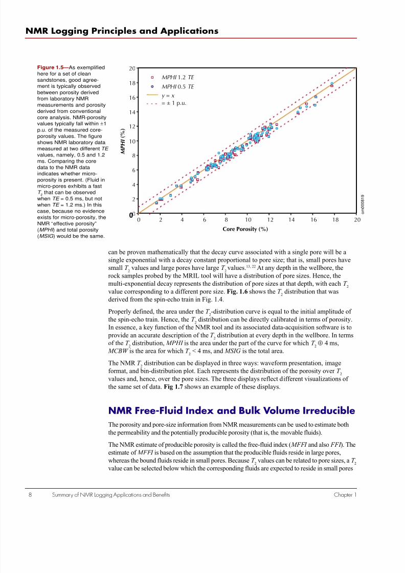
NMR porosity and a Helium Boyles Law porosity is better than 1 p.u. Fig 1.5 illustrates such
an agreement.
NMR T 2
Distribution
The amplitude of the spin-echo-train decay can be fit very well by a sum of decaying
exponentials, each with a different decay constant. The set of all the decay constants forms
the decay spectrum or transverse-relaxation-time (T 2) distribution. In water-saturated rocks, it
7/28/2019 NMR Logging Principles and Applications
http://slidepdf.com/reader/full/nmr-logging-principles-and-applications 26/253
NMR Logging Principles and Applications
8 Summary of NMR Logging Applications and Benefits Chapter 1
can be proven mathematically that the decay curve associated with a single pore will be a
single exponential with a decay constant proportional to pore size; that is, small pores have
small T 2
values and large pores have large T 2values.13, 22 At any depth in the wellbore, the
rock samples probed by the MRIL tool will have a distribution of pore sizes. Hence, the
multi-exponential decay represents the distribution of pore sizes at that depth, with each T 2
value corresponding to a different pore size. Fig. 1.6 shows the T 2
distribution that was
derived from the spin-echo train in Fig. 1.4.
Properly defined, the area under the T 2-distribution curve is equal to the initial amplitude of
the spin-echo train. Hence, the T 2
distribution can be directly calibrated in terms of porosity.
In essence, a key function of the NMR tool and its associated data-acquisition software is to
provide an accurate description of the T 2
distribution at every depth in the wellbore. In terms
of the T 2
distribution, MPHI is the area under the part of the curve for which T 2 ⊕ 4 ms,
MCBW is the area for which T 2
< 4 ms, and MSIG is the total area.
The NMR T 2
distribution can be displayed in three ways: waveform presentation, image
format, and bin-distribution plot. Each represents the distribution of the porosity over T 2
values and, hence, over the pore sizes. The three displays reflect different visualizations of
the same set of data. Fig 1.7 shows an example of these displays.
NMR Free-Fluid Index and Bulk Volume Irreducible
The porosity and pore-size information from NMR measurements can be used to estimate both
the permeability and the potentially producible porosity (that is, the movable fluids).
The NMR estimate of producible porosity is called the free-fluid index ( MFFI and also FFI ). The
estimate of MFFI is based on the assumption that the producible fluids reside in large pores,
whereas the bound fluids reside in small pores. Because T 2values can be related to pore sizes, a T
2
value can be selected below which the corresponding fluids are expected to reside in small pores
20
18
16
14
12
10
8
6
4
2
0 2 4 6 8 10 12 14 16 18 20
M P H I
( % )
Core Porosity (%)
00
MPHI TE 0.5
MPHI TE 1.2
y x == ± 1 p.u.
Figure 1.5 —As exemplified
here for a set of clean
sandstones, good agree-
ment is typically observed
between porosity derived
from laboratory NMRmeasurements and porosity
derived from conventional
core analysis. NMR-porosity
values typically fall within ±1
p.u. of the measured core-
porosity values. The figure
shows NMR laboratory data
measured at two different TE
values, namely, 0.5 and 1.2
ms. Comparing the core
data to the NMR data
indicates whether micro-
porosity is present. (Fluid in
micro-pores exhibits a fast
T 2
that can be observed
whenTE
= 0.5 ms, but notwhen TE = 1.2 ms.) In this
case, because no evidence
exists for micro-porosity, the
NMR “effective porosity”
(MPHI ) and total porosity
(MSIG ) would be the same.
o m
0 0 0 8
1 9

7/28/2019 NMR Logging Principles and Applications
http://slidepdf.com/reader/full/nmr-logging-principles-and-applications 27/253
Summary of NMR Logging Applications and Benefits
Halliburton Energy Service
Chapter 1
2.00
1.80
1.60
1.40
1.20
1.00
0.80
0.60
0.40
0.20
0.1 1 10 100 1,000 10,000
I n c r e m e n t a l P o r o s i t y ( % )
T 2 RelaxationTime (ms)
00.00
Figure 1.6 —Through the
mathematical process of
inversion, the spin-echo
decay data can be con-
verted to a T 2
distribution.
This distribution is the “mostlikely” distribution of T
2
values that produce the
echo train. (The T 2
distribution shown here
corresponds to the spin-
echo train of Fig. 1.4.) With
proper calibration, the area
under the T 2-distribution
curve is equal to the
porosity. This distribution
will correlate with a pore-
size distribution when the
rock is 100% water-
saturated. However, if
hydrocarbons are present,
theT
2 distribution will bealtered depending on the
hydrocarbon type, viscosity,
and saturation.
o m
0 0 0 8 2 0
and above which the corresponding fluids are expected to reside in larger pores. This T 2
value is
called the T 2cutoff (T
2cutoff ).23, 24
Through the partitioning of the T 2
distribution, T 2cutoff
divides MPHI into free-fluid index ( MFFI )
and bound-fluid porosity, or bulk volume irreducible ( BVI ), as shown in Figs. 1.8 and 1.9.
The T 2cutoff
can be determined with NMR measurements on water-saturated core samples.
Specifically, a comparison is made between the T 2
distribution of a sample in a fully water-
saturated state, and the same sample in a partially saturated state, the latter typically being
attained by centrifuging the core at a specified air-brine capillary pressure.23 Although
capillary pressure, lithology, and pore characteristics all affect T 2cutoff
values, common practice
establishes local field values for T 2cutoff
. For example, in the Gulf of Mexico, T 2cutoff
values of
33 and 92 ms are generally appropriate for sandstones and carbonates, respectively.23
Generally though, more accurate values are obtained by performing measurements on core
samples from the actual interval logged by an MRIL tool.
NMR Permeability
NMR relaxation properties of rock samples are dependent on porosity, pore size, pore-fluid properties and mineralogy. The NMR estimate of permeability is based on theoretical models
that show that permeability increases with both increasing porosity and increasing pore
size.24–29 Two related kinds of permeability models have been developed. The free-fluid or
Coates model can be applied in formations containing water and/or hydrocarbons. The
average-T 2
model can be applied to pore systems containing only water.30 Measurements on
core samples are necessary to refine these models and produce a model customized for local
use. Fig. 1.10 shows that the decay of an echo train contains information related to formation
permeability. Fig. 1.11 shows how the Coates model can be calibrated with laboratory core
data. Fig. 1.12 demonstrates MRIL permeability derived from a customized Coates model.

7/28/2019 NMR Logging Principles and Applications
http://slidepdf.com/reader/full/nmr-logging-principles-and-applications 28/253
NMR Logging Principles and Applications
10 Summary of NMR Logging Applications and Benefits Chapter 1
Figure 1.7 —T 2
distributions
are displayed in three ways
on this log: A plot of the
cumulative amplitudes from
the binned T 2-distribution in
Track 1, a color image of thebinned T
2-distribution in
Track 3, and a waveform
presentation of the same
information in Track 4. The
T 2-distribution typically
displayed for MRIL data
corresponds to binned
amplitudes for exponential
decays at 0.5, 1, 2, 4, 8, 16,
32, 64, 128, 256, 512, and
1024 ms when MSIG is
shown and from 4 ms to
1024 ms when MPHI is
shown. The 8-ms bin, for
example, corresponds to
measurements madebetween 6 and 12 ms.
Because logging data are
much noisier than laboratory
data, only a comparatively
coarse T 2-distribution can be
created from MRIL log data.
o m
0 0 1 5 9 8

7/28/2019 NMR Logging Principles and Applications
http://slidepdf.com/reader/full/nmr-logging-principles-and-applications 29/253
Summary of NMR Logging Applications and Benefits 1
Halliburton Energy Service
Chapter 1
NMR Properties of Reservoir Fluids
Clay-bound water, capillary-bound water, and movable water occupy different pore sizes and
locations. Hydrocarbon fluids differ from brine in their locations in the pore space, usually
occupying the larger pores. They also differ from each other and brine in viscosity and
diffusivity. NMR logging uses these differences to characterize the fluids in the pore space.
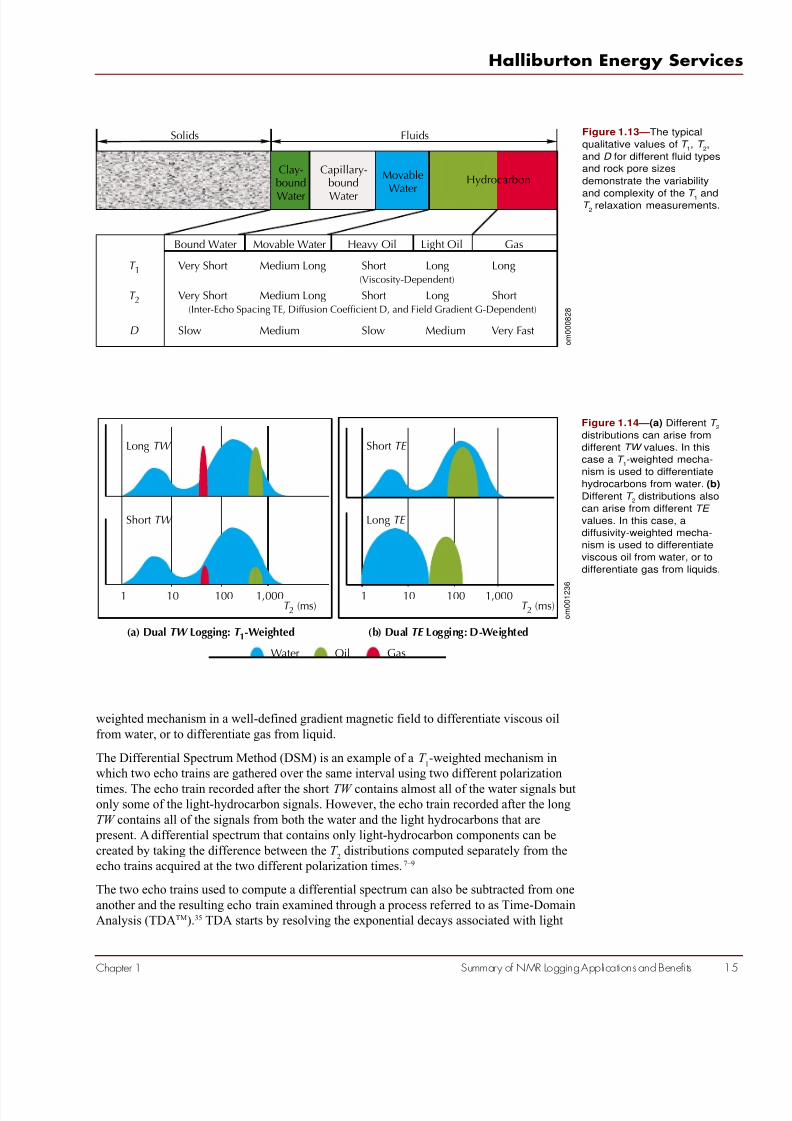
Fig. 1.13 qualitatively indicates the NMR properties of different fluids found in rock pores.31 – 34
In general, bound fluids have very short T 1
and T 2
times, along with slow diffusion (small D)
that is due to the restriction of molecular movement in small pores. Free water commonlyexhibits medium T
1, T
2, and D values. Hydrocarbons, such as natural gas, light oil, medium-
viscosity oil, and heavy oil, also have very different NMR characteristics. Natural gas
exhibits very long T 1
times but short T 2
times and a single-exponential type of relaxation
decay. NMR characteristics of oils are quite variable and are largely dependent on oil
viscosities. Lighter oils are highly diffusive, have long T 1
and T 2
times, and often exhibit a
single-exponential decay. As viscosity increases and the hydrocarbon mix becomes more
complex, diffusion decreases, as do the T 1
and T 2
times, and events are accompanied by
increasingly complex multi-exponential decays. Based on the unique NMR characteristics of
the signals from the pore fluids, applications have been developed to identify and, in some
cases, quantify the type of hydrocarbon present.
NMR Hydrocarbon TypingDespite the variability in the NMR properties of fluids, the locations of signals from differ-
ent types of fluids in the T 2
distribution can often be predicted or, if measured data are
available, identified. This capability provides important information for NMR data interpre-
tation and makes many applications practical.
Fig. 1.14 shows two methods for differentiating fluids. In one method, different TW values
are used with a T 1-weighted mechanism to differentiate light hydrocarbons (light oil or gas, or
both) from water. In the second method, different TE values are used with a diffusivity-
Figure 1.8 —The T 2
distribution is composed of
movable (MFFI ) and immov-
able (BVI and MCBW )
components. Because pore
size is the primary control-ling factor in establishing the
amount of fluid that can
potentially move, and
because the T 2
spectrum is
often related to pore-size
distribution, a fixed T 2
value
should directly relate to a
pore size at and below which
fluids will not move. This
information is used to
decompose MPHI into MFFI
and BVI .
o m
0 0 0 8 2 1
2.00
1.80
1.60
1.40
1.20
1.00
0.80
0.60
0.40
0.20
0.1 1 10 100 1,000 10,000
I n c r e m e n t a l P o r o s i t y ( % )
T 2 Relaxation Time (ms)
00.00
Standard f ixed cutoff Relates to a capillary pressureor pore radius
T 2
Bulk Volume Irreducible ( )and Clay-Bound Water ( )
BVI
MCBW
Free Fluid Index ( )MFFI

7/28/2019 NMR Logging Principles and Applications
http://slidepdf.com/reader/full/nmr-logging-principles-and-applications 30/253
NMR Logging Principles and Applications
12 Summary of NMR Logging Applications and Benefits Chapter 1
Figure 1.9 —This Gulf of
Mexico silty-sand formation
illustrates the variability of
BVI (Track 4). A coarsening-
upward sequence from
X160 to X255 is apparentbased upon the increase of
BVI and gamma ray with
depth. If the free fluid were
predominantly hydrocarbon,
then the increased irreduc-
ible water deeper in the
interval would account for
the observed reduction in
the logged resistivity. What
appears at first sight to be a
transition zone from X190
to X255 could actually be
just a variation of grain size
with depth.
o m
0 0 1 5 9 9

7/28/2019 NMR Logging Principles and Applications
http://slidepdf.com/reader/full/nmr-logging-principles-and-applications 31/253
Summary of NMR Logging Applications and Benefits 1
Halliburton Energy Service
Chapter 1
40
35
30
25
20
15
10
5
0-5
0
50 100 150 200 250
MPHI FFI BVI PERM = 36, = 30, = 6, = 4,200 md
MPHI FFI BVI PERM = 36, = 6, = 30, = 6.7 md
Porosity(p.u.)
Time (ms)
Figure 1.10 —Two echo
trains were obtained from
formations with different
permeability. Both forma-
tions have the same porosity
but different pore sizes. Thisdifference leads to shifted T
2
distributions, and therefore
to different values of the
ratio of MFFI to BVI . The
permeabilities computed
from the Coates model
k = [(MPHI / C )2(MFFI / BVI )]2,
where k is formation
permeability and C is a
constant that depends on
the formation also are
indicated in the figure.
Figure 1.11 —A crossplot
that utilizes core data can
be used to determine the
constant C in the Coates
permeability model.
o m
0 0 0 8 2 4
o m
0 0 0 8 2 6
7/28/2019 NMR Logging Principles and Applications
http://slidepdf.com/reader/full/nmr-logging-principles-and-applications 32/253
NMR Logging Principles and Applications
14 Summary of NMR Logging Applications and Benefits Chapter 1
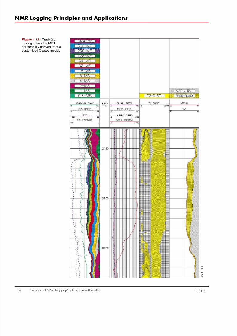
Figure 1.12 —Track 2 of
this log shows the MRIL
permeability derived from a
customized Coates model.
o m
0 0 1 6 0 0
7/28/2019 NMR Logging Principles and Applications
http://slidepdf.com/reader/full/nmr-logging-principles-and-applications 33/253
Summary of NMR Logging Applications and Benefits 1
Halliburton Energy Service
Chapter 1
Figure 1.14 —(a) Different T 2
distributions can arise from
different TW values. In this
case a T 1-weighted mecha-
nism is used to differentiate
hydrocarbons from water. (b)
Different T 2
distributions also
can arise from different TE
values. In this case, a
diffusivity-weighted mecha-
nism is used to differentiate
viscous oil from water, or to
differentiate gas from liquids.
T 2 (ms)
Short TE
Long TE
(b) Dual Logging: D-WeightedTE
Long TW
Short TW
T 2 (ms)
(a) Dual Logging: -WeightedTW T 1
1 110 10100 1001,000 1,000
GasWater Oil
o m
0 0 1 2 3
6
Figure 1.13 —The typical
qualitative values of T 1, T
2,
and D for different fluid types
and rock pore sizes
demonstrate the variability
and complexity of the T 1 andT
2relaxation measurements.
Solids Fluids
MovableWater
Capillary-bound
Water
Clay-bound
Water
Hydrocarbon
GasLight OilHeavy OilMovable WaterBound Water
T 1 Very Short Medium Long Short(Viscosity-Dependent)
Long Long
T 2 Very Short Medium Long Short(Inter-Echo Spacing TE, Diffusion Coefficient D, and Field Gradient G-Dependent)
Long Short
D Slow Medium Slow Medium Very Fast o m
0 0 0 8 2 8
weighted mechanism in a well-defined gradient magnetic field to differentiate viscous oil
from water, or to differentiate gas from liquid.
The Differential Spectrum Method (DSM) is an example of a T 1-weighted mechanism in
which two echo trains are gathered over the same interval using two different polarization
times. The echo train recorded after the short TW contains almost all of the water signals butonly some of the light-hydrocarbon signals. However, the echo train recorded after the long
TW contains all of the signals from both the water and the light hydrocarbons that are
present. A differential spectrum that contains only light-hydrocarbon components can be
created by taking the difference between the T 2
distributions computed separately from the
echo trains acquired at the two different polarization times.7–9
The two echo trains used to compute a differential spectrum can also be subtracted from one
another and the resulting echo train examined through a process referred to as Time-Domain
Analysis (TDATM).35 TDA starts by resolving the exponential decays associated with light

7/28/2019 NMR Logging Principles and Applications
http://slidepdf.com/reader/full/nmr-logging-principles-and-applications 34/253
NMR Logging Principles and Applications
16 Summary of NMR Logging Applications and Benefits Chapter 1
hydrocarbons (oil and/or gas), thereby confirming the presence of these fluids, and then
provides estimates of the fluid volumes. TDA is a more robust process than DSM.
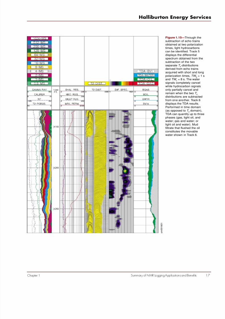
The log in Fig. 1.15 provides an example combining both DSM and TDA results. Because
NMR analysis does not rely on formation water salinity to obtain water saturation, it has an
advantage over conventional resistivity analysis in mixed or unknown salinity conditions.
This feature can be extremely useful in waterflood projects to evaluate residual oil saturation
( ROS ) after the waterflood or to look for bypassed oil.
NMR Enhanced Water Saturation withResistivity Data
Because resistivity tools have a large depth of investigation, a resistivity-based water-
saturation model is preferred for determining water saturation in the virgin zone of a forma-
tion. However, resistivity measurements cannot distinguish between capillary-bound water
and movable water. This lack of contrast makes it difficult to recognize hydrocarbon-
productive low-resistivity and/or low-contrast pay zones from data provided by traditionallogging suites.
The unique information, such as BVI and MCBW , provided by NMR logging can significantly
enhance the estimation of resistivity-based water saturation and can greatly assist in the
recognition of pay zones that will produce water-free.
Through an MRI analysis process referred to as “MRIANTM”,36 the NMR data and the deep-
resistivity data are integrated to determine whether producible water is in the virgin zone, or
whether an interval with high water saturation may actually produce water-free hydrocarbons.
The log shown in Fig. 1.16 includes MRIAN results.
MRIL Application ExamplesMRIL Porosity and Permeability
Fig. 1.17 presents data from a shaly sand formation in Egypt. Track 1 contains MRIL
permeability (green curve) and core permeability (red asterisks). Track 2 contains MRIL
porosity (blue curve) and core porosity (black asterisks). In this reservoir, the highly variable
grain sizes lead to a considerable variation in rock permeability. Capillary-pressure measure-
ments on rock samples yielded a good correlation between the pore bodies and the pore
throat structures. This correlation indicates that the NMR T 2
distribution is a good representa-
tion of the pore throat size distribution when the pores are 100% water-saturated.
Fig. 1.18 shows an MRIL log through a massive low-porosity (approximately 10 p.u.), low-
permeability (approximately 1 to 100 md) sandstone reservoir in Australia’s Cooper basin.23
Track 1 contains gamma ray and caliper logs. Track 2 contains deep- and shallow-readingresistivity logs. Track 3 presents the MRIL calculated permeability and core permeability.
Track 4 shows the MRIL porosity response, neutron and density porosity readings (based on
a sandstone matrix), and core porosity. This well was drilled with a potassium chloride (KCl)
polymer mud [48-kppm sodium chloride (NaCl) equivalent] and an 8.5-in. bit. MRIL data
were acquired with TW = 12 s and TE = 1.2 ms.
Over the interval depicted, the log shows a clean sandstone formation at the top, a shaly
sandstone at the bottom, and an intervening shale between the two sandstones. Agreement
between MPHI and the core porosity is good. The slight underestimation of MPHI relative to
7/28/2019 NMR Logging Principles and Applications
http://slidepdf.com/reader/full/nmr-logging-principles-and-applications 35/253
Summary of NMR Logging Applications and Benefits 1
Halliburton Energy Service
Chapter 1
Figure 1.15 —Through the
subtraction of echo trains
obtained at two polarization
times, light hydrocarbons
can be identified. Track 5
displays the differentialspectrum obtained from the
subtraction of the two
separate T 2-distributions
derived from echo trains
acquired with short and long
polarization times, TW S
= 1 s
and TW L
= 8 s. The water
signals completely cancel
while hydrocarbon signals
only partially cancel and
remain when the two T 2
distributions are subtracted
from one another. Track 6
displays the TDA results.
Performed in time domain
(as opposed toT
2 domain),TDA can quantify up to three
phases (gas, light oil, and
water; gas and water; or
light oil and water). Mud
filtrate that flushed the oil
constitutes the movable
water shown in Track 6.
o m
0 0 1 6 0 1

7/28/2019 NMR Logging Principles and Applications
http://slidepdf.com/reader/full/nmr-logging-principles-and-applications 36/253
NMR Logging Principles and Applications
18 Summary of NMR Logging Applications and Benefits Chapter 1
Figure 1.16 —The combination
of conventional deep-resistivity
data with NMR-derived
MCBW , BVI , MFFI , and MPHI
can greatly enhance petro-
physical estimations ofeffective pore volume, water
cut, and permeability. The
MRIAN analysis results
displayed in Track 5 show that
the whole interval from X160
to X255 has a BVI almost
identical to the water satura-
tion interpreted from the
resistivity log. This zone will
likely produce water-free
because of this high BVI .
o m
0 0 1 6 0 2

7/28/2019 NMR Logging Principles and Applications
http://slidepdf.com/reader/full/nmr-logging-principles-and-applications 37/253
Summary of NMR Logging Applications and Benefits 1
Halliburton Energy Service
Chapter 1
Figure 1.17 —These data
from a shaly sand formation
in Egypt show the good
agreement between core
data and MRIL porosity
and permeability.
o m
0 0 1 6 0 3

7/28/2019 NMR Logging Principles and Applications
http://slidepdf.com/reader/full/nmr-logging-principles-and-applications 38/253
NMR Logging Principles and Applications
20 Summary of NMR Logging Applications and Benefits Chapter 1
Figure 1.18 —This low-
porosity, low-permeability
example from South Australia
shows good agreement
between core data and MRIL
porosity and permeability.
o m
0 0 1 6 0 4

7/28/2019 NMR Logging Principles and Applications
http://slidepdf.com/reader/full/nmr-logging-principles-and-applications 39/253
Summary of NMR Logging Applications and Benefits 2
Halliburton Energy Service
Chapter 1
Figure 1.19 —In this gas
reservoir, MRIL porosity is
affected by the hydrogen
index of the pore fluids. A
corrected porosity, either
from another source such asnuclear logs or from MPHI
after HI correction, should
be used for permeability
calculation.
o m
0 0 1 6 0 5

7/28/2019 NMR Logging Principles and Applications
http://slidepdf.com/reader/full/nmr-logging-principles-and-applications 40/253
NMR Logging Principles and Applications
22 Summary of NMR Logging Applications and Benefits Chapter 1
core porosity is attributed to residual gas in the flushed zone. The MRIL permeability curve
was computed using a model customized to this area. The agreement between MRIL perme-
ability and core permeability is very good.
Fig. 1.19 compares core data with MRIL porosity and permeability recorded in a gas
reservoir.23 Track 1 contains gamma ray and caliper logs. Track 2 contains deep- and shallow-
reading resistivity logs. Track 3 presents the MRIL-derived permeability and core permeability.
Track 4 presents the core porosity, MRIL porosity MPHI , neutron and density porosity (based
on a sandstone matrix), BVI from a model customized to this reservoir, and a bulk volume water
(CBVWE ) from resistivity logs. The MRIL log in this example was acquired with a TW = 10 s,
TE = 1.2 ms, and NE = 500, where NE is the number of echoes per echo train.
A gas/water contact at X220 is easily identified on the resistivity logs. Immediately above the
contact, a large gas crossover (yellow) is observed between the neutron and density logs. A
decrease in MRIL porosity occurs here because of the hydrogen-index effect of the unflushed
gas. Accurate data for BVI and MFFI are important for permeability calculations with the
Coates model. The MPERM curve in Track 3 was calculated from the Coates model: MPHI was
used for porosity, and the difference between MPHI and BVI was used for MFFI . Used in this
way, the Coates model will give good estimates of permeability when the MRIL porosity isunaffected by gas. In zones where the MRIL porosity is affected by gas, MPERM is pessimistic
because the difference between MPHI , and BVI underestimates MFFI . In this situation, the
difference between BVI and the porosity obtained from the nuclear logs gives a better estimate
of MFFI for calculating permeability The PMRI curve was computed in this manner. It is a
more reasonable representation of permeability in the gas zones and in this example, matched
very well with the core permeability. Below the gas/water contact, MRIL porosity and perme-
ability match core data quite well.
Low-Resistivity Reservoir Evaluation
An interval from a Gulf of Mexico well has been used several times throughout this chapter to
illustrate various MRIL measurements (Figs. 1.7, 1.9, 1.12, 1.15, and 1.16). The same well is
now discussed in the context of a specific case study.
The reservoir penetrated by the well consists of a massive medium- to fine-grained sandstone
formation, which developed from marine shelf sediments. Intense bioturbation is observed
within the formation. Air permeability typically ranges between 1 and 200 md, with core
porosity varying between 20 and 30 p.u. The upper portion of the reservoir (Zone A) has higher
resistivity (approximately 1 ohm-m) than that of the lower reservoir (Zone B, approximately 0.5
ohm-m). The produced hydrocarbons are light oil with viscosity from 1 to 2 cp. The well was
drilled with water-based mud. Conventional logs are shown in Fig. 1.20. MRIL results from
both TDA and MRIAN are illustrated in Fig. 1.21.
The operator was concerned about the decrease in resistivity in the lower portion of the
reservoir. The question was whether the decrease was due to textural changes (smaller grain
sizes, in which case the well might produce free of water) or to an increase in the volume of
movable water. The ability to reliably answer this question could have significant implications
on reserve calculations, well-completion options, and future field-development decisions. An
additional piece of key information for this type of reservoir is that the actual cumulative
production often far exceeds the initial calculated recoverable reserves based on a water-
saturation cutoff of 60%. If the entire zone in question were actually at irreducible water
saturation, then the total net productive interval could be increased from 25 to 70 ft. The
resulting increase in net hydrocarbon pore volume would be more than 200%, and expected
recoverable reserves would increase significantly.

7/28/2019 NMR Logging Principles and Applications
http://slidepdf.com/reader/full/nmr-logging-principles-and-applications 41/253
Summary of NMR Logging Applications and Benefits 2
Halliburton Energy Service
Chapter 1
Figure 1.20 —Conventional
logs (SP, resistivity, and
neutron/density) suggested
that the upper part of the
sand (XX160 to XX185)
would possibly produce withhigh water cut, but that the
lower part of the sand
(XX185 to XX257) is
probably wet.
o m
0 0 1 6 0 6

7/28/2019 NMR Logging Principles and Applications
http://slidepdf.com/reader/full/nmr-logging-principles-and-applications 42/253
NMR Logging Principles and Applications
24 Summary of NMR Logging Applications and Benefits Chapter 1
Figure 1.21 —MRIL data
were acquired in the well of
Fig. 1.20 and were used in
DSM, TDA, and MRIAN
analyses. The MRIAN
results (Track 7) indicatethat both the upper and
lower intervals have high
water saturation, but that the
formation water is at
irreducible conditions. Thus,
the zone should not produce
any formation water. The
entire zone has permeability
in excess of 100 md (Track
2). The TDA analysis (Track
6) determined oil saturation
in the flushed zone to be in
the 35 to 45% range. With
this information, the operator
perforated the entire interval
and recorded an initialproduction rate of 2,000
BOPD with no water influx.
o m
0 0 1 6 0 7

7/28/2019 NMR Logging Principles and Applications
http://slidepdf.com/reader/full/nmr-logging-principles-and-applications 43/253
Summary of NMR Logging Applications and Benefits 2
Halliburton Energy Service
Chapter 1
MRIL logs were incorporated into the logging suite for two principal reasons:
1. To distinguish zones of likely hydrocarbon production from zones of likely water
production by establishing the bulk volume of irreducible water ( BVI ) and the
volume of free fluids ( MFFI ).
2. To improve the estimation of recoverable reserves by defining the producible
interval
The MRIL data acquired in this well were to include total porosity to determine clay-bound
water, capillary-bound water, and free fluids. Dual-TW logging was to be used to distinguish
and quantify hydrocarbons.
The MRIL data in Fig. 1.21 helped determine that the resistivity reduction was due to a
change in grain size and not to the presence of movable water. The two potential types of
irreducible water that can cause a reduction in measured resistivity are clay-bound water
(whose volume is designated by MCBW ) and capillary-bound water (whose volume is
indicated by BVI ). The MRIL clay-bound-water measurement (Track 3) indicates that the
entire reservoir has very low MCBW . The MRIL BVI curve (Track 7) indicates a coarsening-
upward sequence ( BVI increases with depth). The increase in BVI and the corresponding
reduction in resistivity are thus attributed to the textural change. Results of the TDA (Track
6) and TDA/MRIAN (Track 7) combination analysis imply that the entire reservoir contains
no significant amount of movable water and is at irreducible condition.
Based on these results, the operator perforated the interval from XX163 to XX234. The
initial production of 2,000 BOPD was water-free and thus confirmed the MRIL analysis.
A difference can be found between the TDA and TDA/MRIAN results in Fig. 1.21. The TDA
shows that the free fluids include both light oil and water, whereas the TDA/MRIAN results
show that all of the free fluids are hydrocarbons. This apparent discrepancy is simply due to
the different depth of investigation of different logging measurements. TDA saturation
reflects the flushed zone as seen by MRIL measurement. The TDA/MRIAN combination
saturation reflects the virgin zone as seen by deep-resistivity measurements. Because water- based mud was used in this well, some of the movable hydrocarbons are displaced in the
invaded zone by the filtrate from the water-based mud.
MRIL Acquisition Data Sets
The unique capacity of the MRIL logging tool to measure multiple quantities needed for
prospect evaluation and reservoir modeling depends on making multiple NMR measurements
on the “same” rock volume using different activations. These different activations can usually
be used during the same logging run with a multiple-frequency tool such as the MRIL Prime.2
Three general categories of activation sets are in common use: total porosity, dual TW , and
dual TE .
A total-porosity activation set acquires two echo trains to obtain the total porosity MSIG . Toacquire one of the echo trains, the tool uses TE = 0.9 or 1.2 ms and a long TW to achieve
complete polarization. This echo train provides the “effective porosity” MPHI . To acquire the
second echo train, the tool uses TE = 0.6 ms and a short TW that is only long enough to
achieve complete polarization of the fluids in the small pores. The second echo train is
designed to provide the porosity MCBW contributed by pores of the same size as clay pores.16
A dual-TW activation is primarily used to identify light hydrocarbons (gas and light oil).
Typically, measurements are made with TW = 1 and 8 s, and TE = 0.9 or 1.2 ms. The water
signal is contained in both activations, but light hydrocarbons (which have long T 1
values)

7/28/2019 NMR Logging Principles and Applications
http://slidepdf.com/reader/full/nmr-logging-principles-and-applications 44/253
NMR Logging Principles and Applications
26 Summary of NMR Logging Applications and Benefits Chapter 1
have a greatly suppressed signal in the activation with TW = 1 s. The presence of a signal in
the difference of the measurements is a very robust indicator of gas or light oils.37
A dual-TE activation is primarily used to identify the presence of viscous oil, which has a
small diffusion constant relative to water. This type of activation set has a long TW and has
TE values of 0.9 or 1.2 ms and 3.6 or 4.8 ms. For this set, the fluid with the larger diffusion
constant (water) has a spectrum shifted more to earlier times than the fluid with the smaller
diffusion constant (viscous oil). The presence in the spectra of a minimally shifted portion
identifies high-viscosity oil in the formation.38, 39
MRIL Response in Rugose Holes
As shown in Fig. 1.22, an MRIL tool responds to the materials in a series of cylindrical
shells, each approximately 1 mm thick. Borehole or formation materials outside these shells
have no influence on the measurements, a situation similar to medical MRI. Hence, if the
MRIL tool is centralized in the wellbore, and the diameter of any washout is less than the
diameter of the inner sensitive shell, then the MRIL tool will respond solely to the NMR
properties of formation. In other words, borehole rugosity and moderate washouts will not
affect MRIL measurements. Fig. 1.23 provides an example of an MRIL log run in a
rugose borehole.
The diameters of the response shells for an MRIL tool are dependent on operating frequency
and tool temperature. For an MRIL tool, the highest frequency of operation is 750 kHz,
which corresponds to a diameter of investigation of approximately 16 in. at 100°F. At the
lowest operating frequency of 600 kHz, the diameter of investigation is about 18 in. at 100°F.
Charts that illustrate the dependence of the depth of investigation on operating frequency and
tool temperature have been published.40, 41
NMR Logging Applications Summary Case studies and theory have shown that MRIL tools furnish powerful data for
• distinguishing low-resistivity/low-contrast pay zones
• evaluating complex-lithology oil and/or gas reservoirs
• identifying medium-viscosity and heavy oils
• studying low-porosity/low-permeability formations
• determining residual oil saturation
• enhancing stimulation design
In particular, NMR data provide the following valuable information:
• mineralogy-independent porosity
• porosity distribution, complete with a pore-size distribution in water-saturated
formations
• bulk volume irreducible and free fluid when a reliable T 2cutoff
value is available

7/28/2019 NMR Logging Principles and Applications
http://slidepdf.com/reader/full/nmr-logging-principles-and-applications 45/253
Summary of NMR Logging Applications and Benefits 2
Halliburton Energy Service
Chapter 1
Figure 1.22 —The depth of
investigation of an MRIL tool
is about 18 in. when
operating at low frequency
and about 16 in. at high
frequency. Thus, in a 12-in.borehole, rugosity with an
amplitude smaller than 2 in.
will not affect the
MRIL signal.
o m
0 0 0 8 3
4
Figure 1.23 —An MRIL tool
can often provide reliable
data in highly rugose holes
where traditional porosity
logs cannot. In thisexample, both neutron and
density measurements are
very sensitive to rugosity,
and only the MRIL tool
provides the correct
porosity. Additionally,
because MRIL porosity is
lithology-independent, the
change from limestone in
an upper zone on the
displayed log to sandstone
in a lower zone has no
effect on the accuracy of
the MRIL porosity values.
An MRIL-Prime tool was
run at a logging speed of 24ft/min to acquire these data.
o m
0 0 1 6 0 8

7/28/2019 NMR Logging Principles and Applications
http://slidepdf.com/reader/full/nmr-logging-principles-and-applications 46/253
NMR Logging Principles and Applications
28 Summary of NMR Logging Applications and Benefits Chapter 1
FluidProperties
MRIL-Prime
RDTReservoirDecisionCenter
SamplePoints
ReservoirLocation
MRIL / LWD
Figure 1.24 —The LWD
NMR device provides
information for locating the
reservoir while drilling. The
MRIL-Prime furnishes
information for producibilityanalysis after invasion has
occurred. The RDT NMR
device yields information for
determining fluid NMR
properties at reservoir
conditions.
o m
0 0 0 8 3 7
• permeability, determined from the free-fluid index and the bulk volume irreducible
or average T 2
• hydrocarbon typing through the use of (1) T 1-weighted contrasts for water, gas,
and/or light oil, (2) diffusivity-weighted contrasts for water and viscous oil, and
(3) NMR enhanced water saturation calculations for the virgin zone
Although this monograph primarily addresses NMR wireline logging, NMR tools are also
used in other parts of the prospecting and reservoir-characterization process. These tools
include a logging-while-drilling (LWD) NMR tool for early reservoir identification and
properties estimation, and an NMR device built into a reservoir description tool (RDTTM),
advanced formation testing and fluid-sampling device. The LWD tool uses the same prin-
ciples as the MRIL tool, but provides information earlier and on uninvaded rocks. The RDT
device provides fluid-property information at downhole reservoir conditions. All of the
information from the LWD NMR tool, the MRIL tool, and the RDT NMR device can then be
integrated at a reservoir decision center to give a more complete analysis. Fig. 1.24 provides
a schematic of this process.
References
1. Coates, G.R., et al., 1991, The MRIL in Conoco 33-1—an investigation of a new
magnetic resonance imaging log, paper DD, 32nd Annual SPWLA Logging Symposium
Transactions, 24 p.
2. Prammer, M.G., et al., 1998, A new multiband generation of NMR logging tools, SPE
49011, 1998 SPE Annual Technical Conference and Exhibition Proceedings, p. 237–243.

7/28/2019 NMR Logging Principles and Applications
http://slidepdf.com/reader/full/nmr-logging-principles-and-applications 47/253
Summary of NMR Logging Applications and Benefits 2
Halliburton Energy Service
Chapter 1
3. Vinegar, H.J., 1986, X-ray CT and NMR imaging of rocks, SPE 15277, Journal of
Petroleum Technology, v. 38, no. 3, p. 257–259. Later reprinted in 1994 in Petrophysics,
SPE Reprint Series No. 39, p. 115–117.
4. Hearst, J.R., and Nelson, P.H., 1985, Well Logging for Physical Properties, McGraw-Hill
Book Company, New York.
5. Bassiouni, Z., 1994, Theory, Measurement, and Interpretation of Well Logs, SPE
Textbook Series, v. 4.
6. Miller, M.N., et al., 1990, Spin-echo magnetic-resonance logging—porosity and free-
fluid index, SPE 20561, 1990 SPE Annual Technical Conference and Exhibition Pro-
ceedings, v.Ω (Formation evaluation and reservoir geology), p. 321–334.
7. Akkurt, R., et al., 1995, NMR logging of natural gas reservoirs, paper N, 36th Annual
SPWLA Logging Symposium Transactions, 12 p. Also published in 1996 in The Log
Analyst , v. 37, no. 5, p. 33–42.
8. Prammer, M.G., et al., 1995, Lithology-independent gas detection by gradient-NMR
logging, SPE 30562, 1995 SPE Annual Technical Conference and Exhibition Proceed-ings, v. Ω (Formation evaluation and reservoir geology), p. 325–336.
9. Moore, M.A., and Akkurt, R., 1996, Nuclear magnetic resonance applied to gas detection
in a highly laminated Gulf of Mexico turbidite invaded with synthetic oil filtrate,
SPE 36521, 1996 SPE Annual Technical Conference and Exhibition Proceedings, v.Ω
(Formation evaluation and reservoir geology), p. 305–310.
10. Mardon, D., et al., 1996, Characterization of light hydrocarbon-bearing reservoirs by
gradient NMR well logging—a Gulf of Mexico case study, SPE 36520, 1996 SPE Annual
Technical Conference and Exhibition Proceedings, v. Ω (Formation evaluation and
reservoir geology), p. 295–304. Also published in 1996 in condensed form in Journal of
Petroleum Technology, v. 48, no. 11, p. 1035–1036.
11. Looyestijn, W., 1996, Determination of oil saturation from diffusion NMR logs, paper SS, 37th Annual SPWLA Logging Symposium Transactions, 14 p.
12. Morriss, C.E., et al., 1994, Hydrocarbon saturation and viscosity estimation from NMR
logging in the Belridge diatomite, paper C, 35th Annual SPWLA Logging Symposium
Transactions, 24 p. Later published in 1997 in The Log Analyst , v. 38, no. 2, p. 44–59.
13. Brownstein, K.R., and Tarr, C.E., 1979, Importance of classical diffusion in NMR studies
of water in biological cells, Physical Review, Series A, v. 19, p. 2446–2453.
14. Prammer, M.G., 1994, NMR pore size distributions and permeability at the well site,
SPE 28368, 1994 SPE Annual Technical Conference and Exhibition Proceedings, v.Ω
(Formation evaluation and reservoir geology), p. 55–64.
15. Sandor, R.K.J., and Looyestijn, W.J., 1995, NMR logging—the new measurement, Shell
International Petroleum Maatschappij, The Hague, The Netherlands, 8 p.
16. Prammer, M.G., et al., 1996, Measurements of clay-bound water and total porosity by
magnetic resonance logging, SPE 36522, 1996 SPE Annual Technical Conference and
Exhibition Proceedings, v. Ω (Formation evaluation and reservoir geology), p. 111–118.
Also published in 1996 in The Log Analyst , v. 37, no. 5, p. 61–69.
17. Murphy, D.P., 1995, NMR logging and core analysis—simplified, World Oil , v. 216,
no. 4, p. 65–70.

7/28/2019 NMR Logging Principles and Applications
http://slidepdf.com/reader/full/nmr-logging-principles-and-applications 48/253
NMR Logging Principles and Applications
30 Summary of NMR Logging Applications and Benefits Chapter 1
18. Cherry, R., 1997, Magnetic resonance technology and its applications in the oil and gas
industry, part 1, Petroleum Engineer International , v. 70, no. 3, p. 29–35.
19. Marschall, D., 1997, Magnetic resonance technology and its applications in the oil and
gas industry, part 2, Petroleum Engineer International , v. 70, no. 4, p. 65–70.
20. Xiao, L.Z., 1998, NMR Imaging Logging Principles and Applications (in Chinese),
Science Press, Beijing.
21. Fukushima, E., and Roeder, S.B.W., 1981, Experimental Pulse NMR: A Nuts and Bolts
Approach, Addison-Wesley Publishing Company, Advanced Book Program, Reading,
Massachusetts, U.S.A.
22. Kenyon, W.E., 1992, Nuclear magnetic resonance as a petrophysical measurement,
Nuclear Geophysics, v. 6, no. 2, p. 153-171. Later revised and published in 1997 under
the title, Petrophysical principles of applications of NMR logging, in The Log Analyst ,
v. 38, no. 2, p. 21–43.
23. Coates, G., et al., 1997, A new characterization of bulk-volume irreducible using mag-
netic resonance, paper QQ, 38th Annual SPWLA Logging Symposium Transactions, 14 p.Also published in 1997 in DiaLog (London Petrophysical Society), v. 5, no. 6, p. 9–16.
Later revised and published in The Log Analyst , v. 39, no. 1, p. 51–63.
24. Timur, A., 1967, Pulsed nuclear magnetic resonance studies of porosity, movable fluid
and permeability of sandstones, SPE 2045, 42nd Annual Meeting preprint, SPE. Later
published in 1969 in Journal of Petroleum Technology, v. 21, no. 6, p. 775–786.
25. Timur, A., 1968, An investigation of permeability, porosity, and residual water saturation
relationships for sandstone reservoirs, paper J, 9th Annual SPWLA Logging Symposium
Transactions, 18 p. Later published in 1968 in The Log Analyst , v. 9, no. 4, July-August,
p. 8–17. Later reprinted in 1994 in Petrophysics, SPE Reprint Series No. 39, p. 128-137.
26. Timur, A., 1968, Effective porosity and permeability of sandstones investigated through
nuclear magnetic principles, paper K, 9th Annual SPWLA Logging Symposium Transac-tions, 18 p. Later published in 1969 in The Log Analyst , v. 10, no. 1, January-February,
p. 3–11.
27. Ahmed, U., Crary, S.F., and Coates, G.R., 1989, Permeability estimation; the various
sources and their interrelationship, SPE 19604, 1989 SPE Annual Technical Conference
and Exhibition Proceedings, v.Ω (Formation evaluation and reservoir geology), p. 649–
662. Later published in 1990 under the title, The interrelationship between various
permeability measurements, paper I, 1990 International Well Logging Symposium
Transactions, SPWLA, Beijing Chapter, 21 p. Later published in 1991 in Journal of
Petroleum Technology, v. 43, no. 5, p. 578–587. Later reprinted in 1994 in Petrophysics,
SPE Reprint Series No. 39, p. 118–127.
28. Allen, D., et al., 1988, Probing for permeability—An introduction of measurements, The
Technical Review, v. 36, no. 1, p. 6–20.
29. Thompson, A., Katz, A.J., and Krohn, C.E., 1987, The microgeometry and transport
properties of sedimentary rock, Advances in Physics, Vol. 36.
30. Marschall, D., Gardner, J., and Curby, F.M., 1997, MR laboratory measurements—
requirements to assure successful measurements that will enhance MRI log interpretation,
paper SCA 9704, 1997 International Symposium Proceedings, SPWLA, Society of Core
Analysts Chapter-at-Large, 12 p.

7/28/2019 NMR Logging Principles and Applications
http://slidepdf.com/reader/full/nmr-logging-principles-and-applications 49/253
Summary of NMR Logging Applications and Benefits 3
Halliburton Energy Service
Chapter 1
31. Morriss, C.E., et al., 1994, Hydrocarbon saturation and viscosity estimation from NMR
logging in the Belridge diatomite, paper C, 35th Annual SPWLA Logging Symposium
Transactions, 24 p. Later published in 1997 in The Log Analyst , v. 38, no. 2, p. 44–59.
32. Kleinberg, R.L., and Vinegar, H.J., 1996, NMR properties of reservoir fluids, The Log
Analyst , v. 37, no. 6, p. 20–32.
33. Gerritsma, C.J., Oosting, P.H., and Trappeniers, N.J., 1971, Proton spin-lattice relaxation
and self-diffusion in methane, part 2—Experiemental results for proton spin-lattice
relaxation times, Physica, v. 51, p. 381–394.
34. Gerritsma, C.J., and Trappeniers, N.J., 1971, Proton spin-lattice relaxation and self-
diffusion in methanes, part 1, Spin-echo spectrometer and preparation of the methane
samples, Physica, v. 51, p. 365–380.
35. Akkurt, R., Moore, A., and Freeman, J., 1997, Impact of NMR in the development of a
deepwater turbidite field, paper SS, 38th Annual SPWLA Logging Symposium Transac-
tions, 14 p.
36. Coates, G.R., Gardner, J.S., and Miller, D.L., 1994, Applying pulse-echo NMR to shalysand formation evaluation, paper B, 35th Annual SPWLA Logging Symposium Transac-
tions, 22 p.
37. Akkurt, R., Prammer, M., and Moore, A., 1996, Selection of optimal acquisition param-
eters for MRIL logs, paper TT, 37th Annual SPWLA Logging Symposium Transactions,
13 p. Later published in 1996 in The Log Analyst , v. 37, no. 6, p. 43–52.
38. Akkurt, R., et al., 1998, Enhanced diffusion: expanding the range of NMR direct hydro-
carbon-typing applications, paper GG, 39th Annual SPWLA Logging Symposium Transac-
tions, 14 p.
39. Akkurt, R., et al., 1998, Determination of residual oil saturation using enhanced diffu-
sion, SPE 49014, 1998 SPE Annual Technical Conference and Exhibition Proceedings,
v.Ω
(Formation evaluation and reservoir geology), 11 p.40. Chandler, R.N., et al., 1994, Improved log quality with a dual-frequency pulsed NMR
tool, SPE 28365, 1994 SPE Annual Technical Conference and Exhibition Proceedings,
v.Ω (Formation evaluation and reservoir geology), p. 23–35.
41. MRIL Operation Manual , Halliburton, 1998.

7/28/2019 NMR Logging Principles and Applications
http://slidepdf.com/reader/full/nmr-logging-principles-and-applications 50/253
NMR Logging Principles and Applications
32 Summary of NMR Logging Applications and Benefits Chapter 1

7/28/2019 NMR Logging Principles and Applications
http://slidepdf.com/reader/full/nmr-logging-principles-and-applications 51/253
NMR Physics 33
Halliburton Energy Services
Chapter 2
NMR PhysicsThe physical principles on which NMR logging is based are complex.
However, NMR logging measurements and NMR log interpretation
can be understood with a knowledge of a few basic NMR concepts.
These concepts include nuclear magnetism, polarization, T 1
relaxation
time, pulse tipping, free induction decay, spin echoes, T 2
relaxation
time, and CPMG pulse sequences. This chapter is devoted to a
discussion of these concepts. More complete and advanced discussions
of the basics of NMR physics are found in the textbooks referenced at
the end of the chapter.
Nuclear Magnetism
Nuclear magnetic resonance (NMR) refers to the response of atomic
nuclei to magnetic fields. Many nuclei have a net magnetic moment
and angular momentum or spin. In the presence of an external mag-
netic field, an atomic nucleus precesses around the direction of the
external field in much the same way a gyroscope precesses around
the earth’s gravitational field. When these spinning magnetic nuclei
interact with the external magnetic fields, measurable signals can
be produced.
NMR measurements can be made on any nucleus that has an odd number of protons or neutrons or both, such as the nucleus of hydrogen
(1H), carbon (13C), and sodium (23 Na). For most of the nuclei found in
earth formations, the nuclear magnetic signal induced by external
magnetic fields is too small to be detected with a borehole NMR
logging tool. However, hydrogen, which has only one proton and no
neutrons, is abundant in both water and hydrocarbons, has a relatively
large magnetic moment, and produces a strong signal. To date, almost
all NMR logging and NMR rock studies are based on responses of the
nucleus of the hydrogen atom. For this reason, sometimes the word
“nuclear” is dropped from “nuclear magnetic resonance,” and instead
“magnetic resonance” (MR) logging or “magnetic resonance imaging”
(MRI) logging is used. This text will concentrate on proton (i.e.,
hydrogen) NMR.
The nucleus of the hydrogen atom is a proton, which is a small,
positively charged particle with an associated angular momentum or
spin. The spinning proton represents a current loop that generates a
magnetic field (or magnetic moment) with two poles (north and south)
aligned with the spin axis. Therefore, the hydrogen nucleus can be
Chapter 2

7/28/2019 NMR Logging Principles and Applications
http://slidepdf.com/reader/full/nmr-logging-principles-and-applications 52/253
NMR Logging Principles and Applications
34 NMR Physics Chapter 2
considered as a bar magnet whose magnetic axis is aligned with the spin axis of the nucleus,
as illustrated in Fig. 2.1 (left). When many hydrogen atoms are present and no external
magnetic field exists, the hydrogen nuclear spin axes are randomly aligned, as seen in Fig.
2.1 (right).
Polarization
The first step in making an NMR measurement is to align magnetic nuclei with a static
magnetic field, B0. When B
0is applied to a magnetic nucleus, B
0exerts a torque on the
nucleus that acts to align the nuclear spin axis with B0.
When a torque is applied to a spinning object, the axis of the object moves perpendicular to
the torque in a motion called precession, as illustrated in Fig. 2.2 (left). Thus, when B0
is
applied to a magnetic nucleus, the nucleus will precess around B0. The precessional fre-
quency ( f ), called the Larmor frequency, is given by
π2
0 B f
γ = (2.1)
where γ is the gyromagnetic ratio, which is a measure of the strength of the nuclear magne-
tism. For hydrogen, γ /2π = 42.58 MHz/tesla. Other nuclei have other γ values.1
Equation 2.1 shows that the Larmor frequency of a given nucleus is proportional to the
magnitude of the static magnetic field and to the gyromagnetic ratio of the given nucleus. For
a given magnetic field, different nuclear species have different Larmor frequencies (because
of their different gyromagnetic ratios); therefore, the various species can be differentiated on
the basis of these frequencies.
Alternatively, for a given nuclear species, such as hydrogen, the gyromagnetic ratio has a
fixed value, and according to Eq. 2.1, the Larmor frequency is a function of the strength of
the static magnetic field. If the strength of the magnetic field is position-dependent, then the
Figure 2.1—Because oftheir inherent nuclearmagnetism, hydrogennuclei (left) behave asthough they are tiny barmagnets aligned with thespin axes of the nuclei. Inthe absence of an externalmagnetic field, the nuclearmagnetic axes (right) arerandomly aligned.
+
N
S
o m 0 0 0 8 3 8
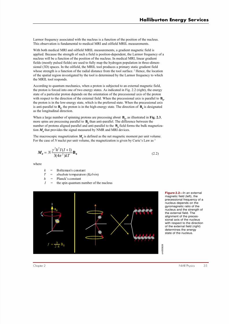
7/28/2019 NMR Logging Principles and Applications
http://slidepdf.com/reader/full/nmr-logging-principles-and-applications 53/253
NMR Physics 35
Halliburton Energy Services
Chapter 2
Larmor frequency associated with the nucleus is a function of the position of the nucleus.
This observation is fundamental to medical MRI and oilfield MRIL measurements.
With both medical MRI and oilfield MRIL measurements, a gradient magnetic field is
applied. Because the strength of such a field is position-dependent, the Larmor frequency of a
nucleus will be a function of the position of the nucleus. In medical MRI, linear gradient
fields (mostly pulsed fields) are used to fully map the hydrogen population in three-dimen-
sional (3D) spaces. In the oilfield, the MRIL tool produces a primary static gradient field
whose strength is a function of the radial distance from the tool surface. 2 Hence, the location
of the spatial region investigated by the tool is determined by the Larmor frequency to which
the MRIL tool responds.
According to quantum mechanics, when a proton is subjected to an external magnetic field,
the proton is forced into one of two energy states. As indicated in Fig. 2.2 (right), the energy
state of a particular proton depends on the orientation of the precessional axis of the proton
with respect to the direction of the external field. When the precessional axis is parallel to B0,
the proton is in the low-energy state, which is the preferred state. When the precessional axis
is anti-parallel to B0, the proton is in the high-energy state. The direction of B
0is designated
as the longitudinal direction.
When a large number of spinning protons are precessing about B0, as illustrated in Fig. 2.3,
more spins are precessing parallel to B0
than anti-parallel. The difference between the
number of protons aligned parallel and anti-parallel to the B0
field forms the bulk magnetiza-
tion M 0 that provides the signal measured by NMR and MRI devices.
The macroscopic magnetization M 0
is defined as the net magnetic moment per unit volume.
For the case of N nuclei per unit volume, the magnetization is given by Curie’s Law as 3
0B
T k
I I h N
)4(3
)1(2
22
π
γ +=
0 M (2.2)
where
k = Boltzman’s constantT = absolute temperature (Kelvin)
h = Planck’s constant
I = the spin quantum number of the nucleus
B0
Many Spins
Β0γ
2 πƒ =
Single Spin
Low Energy
High Energy
ƒ
x
x
zz
y
y
B0
Figure 2.2 —In an externalmagnetic field (left), theprecessional frequency of anucleus depends on thegyromagnetic ratio of thenucleus and the strength ofthe external field. Thealignment of the preces-sional axis of the nucleuswith respect to the direction
of the external field (right)determines the energystate of the nucleus.
o m 0 0 0 8 3 9

7/28/2019 NMR Logging Principles and Applications
http://slidepdf.com/reader/full/nmr-logging-principles-and-applications 54/253
NMR Logging Principles and Applications
36 NMR Physics Chapter 2
M 0
is observable and, according to Eq. 2.2, is proportional to the number of protons, the
magnitude B0
of the applied magnetic field, and the inverse of the absolute temperature.
After the protons are aligned in the static magnetic field, they are said to be polarized.
Polarization does not occur immediately but rather grows with a time constant,4 which is the
longitudinal relaxation time, T 1:
)1()( 10
T
t
z e M t M
−
−=(2.3)
where
t = the time that the protons are exposed to the B0
field
M z (t ) = the magnitude of magnetization at time t , when the direction of B
0is taken
along the z axis
M 0
= the final and maximum magnetization in a given magnetic field
T 1
is the time at which the magnetization reaches 63% of its final value, and three times T 1is
the time at which 95% polarization is achieved . A T 1 relaxation or polarization curve isillustrated in Fig. 2.4. Different fluids, such as water, oil, and gas, have very different T
1
relaxation times.
Figure 2.3— When manyprotons are precessing inan external magneticfield, a net magnetization(M
0) will be exhibited.
o m 0 0 0 8 4 0
om000840.cdr
.eps

7/28/2019 NMR Logging Principles and Applications
http://slidepdf.com/reader/full/nmr-logging-principles-and-applications 55/253
NMR Physics 37
Halliburton Energy Services
Chapter 2
Pulse Tipping and Free Induction Decay
The second step in the NMR measurement cycle is to tip the magnetization from the longitu-
dinal direction to a transverse plane. This tipping is accomplished by applying an oscillating
magnetic field (B1) perpendicular to B
0, the static magnetic field. For effective tipping, the
frequency of B1
must equal the Larmor frequency of the protons relative to B0.
An oscillating magnetic field interacting with protons is illustrated in Fig. 2.5. From the
quantum mechanics point of view, if a proton is at the low-energy state, it may absorb energy
provided by B1 and jump to the high-energy state. The application of B1 also causes the protons to precess in phase with one another. This change in energy state and in-phase
precession caused by B1
is called nuclear magnetic resonance.
0
0 1 2 3 4 5
M(t)/M
0
1-exp(-t/ )T 1
PolarizationTime /T 1
At 3 , recovery is 95%.T 1
1.000.95
Figure 2.4 —T 1-relaxation
(polarization) curvesindicate the degree ofproton alignment, ormagnetization, as a
function of the time that aproton population isexposed to an externalmagnetic field.
o m 0 0 0 8 4 1
ƒ0
ƒ
x
y
B0
B1
B1
z
Low Energy
High Energy
ƒ
Figure 2.5 —For effectiveinteraction with protons(left), the oscillatingmagnetic field B
1must
have a substantialcomponent perpendicularto the static field B
0and
must have frequency ƒ
equal to the proton’sLarmor frequency ƒ
0in the
static field. In this case
(right), the protons willprecess in phase with oneanother and may absorbenergy from the oscillatingfield and change to thehigh-energy state.Nuclear magnetic reso-nance thus occurs.
o m 0 0 0 8 4 4

7/28/2019 NMR Logging Principles and Applications
http://slidepdf.com/reader/full/nmr-logging-principles-and-applications 56/253
NMR Logging Principles and Applications
38 NMR Physics Chapter 2
On a macroscopic level, resonance results in the tipping of the magnetization, which pre-
cesses about B0
at the Larmor frequency. The angle through which the magnetization is
tipped is given by5,6
τ γ θ 1
B= (2.4)
where
θ = tip angle (degrees)
B1
= amplitude of the oscillating field
τ = time over which the oscillating field is applied
The tip angle is thus proportional to the product B1τ , which reflects the energy that B
1sup-
plies to the proton spin system. Increasing the strength of the oscillating field or increasing
the time over which the oscillating field is applied increases the tip angle. The tipping-angle
relationship of Eq. 2.4 is illustrated in Fig. 2.6.
The B1 field used in NMR logging is a pulsed oscillating magnetic field. Angular-pulse terms,such as a π pulse (or 180° pulse) and a π/2 pulse (or 90° pulse), refer to the angle through
which magnetization is tipped by B1.
When an NMR tool applies a 90° B1
pulse to the proton population that the tool has polar-
ized, the protons precess in phase in transverse planes (relative to B0). Macroscopically,
magnetization is tipped 90° and precesses in the transverse plane.
Figure 2.6— The tip angleθ depends on the strengthof the oscillating field B
1
and on the time τ over
which the field is applied.
o m 0 0 0 8 4 5
om000845.cdr
.eps
M
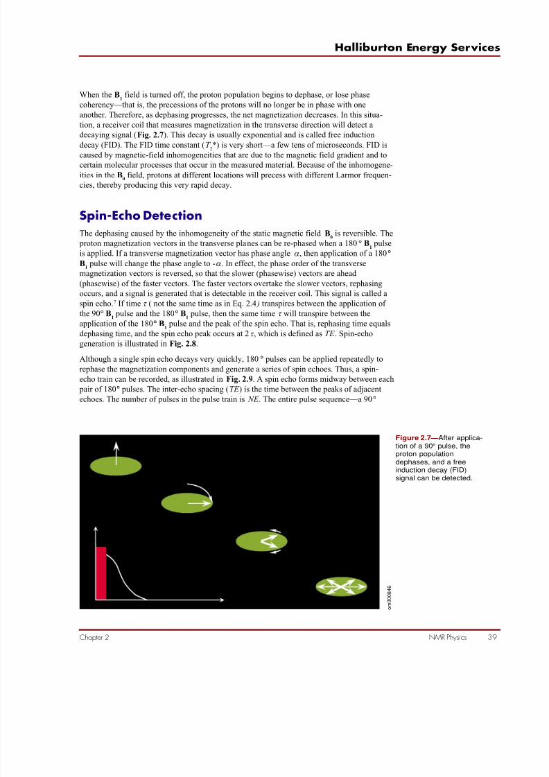
7/28/2019 NMR Logging Principles and Applications
http://slidepdf.com/reader/full/nmr-logging-principles-and-applications 57/253
NMR Physics 39
Halliburton Energy Services
Chapter 2
When the B1
field is turned off, the proton population begins to dephase, or lose phase
coherency—that is, the precessions of the protons will no longer be in phase with one
another. Therefore, as dephasing progresses, the net magnetization decreases. In this situa-
tion, a receiver coil that measures magnetization in the transverse direction will detect a
decaying signal (Fig. 2.7). This decay is usually exponential and is called free inductiondecay (FID). The FID time constant (T
2*) is very short—a few tens of microseconds. FID is
caused by magnetic-field inhomogeneities that are due to the magnetic field gradient and to
certain molecular processes that occur in the measured material. Because of the inhomogene-
ities in the B0
field, protons at different locations will precess with different Larmor frequen-
cies, thereby producing this very rapid decay.
Spin-Echo Detection
The dephasing caused by the inhomogeneity of the static magnetic field B0
is reversible. The
proton magnetization vectors in the transverse planes can be re-phased when a 180° B1
pulse
is applied. If a transverse magnetization vector has phase angle α, then application of a 180°
B1
pulse will change the phase angle to -α. In effect, the phase order of the transverse
magnetization vectors is reversed, so that the slower (phasewise) vectors are ahead (phasewise) of the faster vectors. The faster vectors overtake the slower vectors, rephasing
occurs, and a signal is generated that is detectable in the receiver coil. This signal is called a
spin echo.7 If time τ ( not the same time as in Eq. 2.4 ) transpires between the application of
the 90° B1
pulse and the 180° B1
pulse, then the same time τ will transpire between the
application of the 180° B1
pulse and the peak of the spin echo. That is, rephasing time equals
dephasing time, and the spin echo peak occurs at 2τ , which is defined as TE . Spin-echo
generation is illustrated in Fig. 2.8.
Although a single spin echo decays very quickly, 180° pulses can be applied repeatedly to
rephase the magnetization components and generate a series of spin echoes. Thus, a spin-
echo train can be recorded, as illustrated in Fig. 2.9. A spin echo forms midway between each
pair of 180° pulses. The inter-echo spacing (TE ) is the time between the peaks of adjacent
echoes. The number of pulses in the pulse train is NE . The entire pulse sequence—a 90°
90° Pulse
FID
Time
90° Pulse
Figure 2.7 —After applica-tion of a 90° pulse, theproton populationdephases, and a freeinduction decay (FID)signal can be detected.
o m 0 0 0 8 4 6

7/28/2019 NMR Logging Principles and Applications
http://slidepdf.com/reader/full/nmr-logging-principles-and-applications 58/253
NMR Logging Principles and Applications
40 NMR Physics Chapter 2
pulse followed by a long series of 180° pulses—is called a CPMG sequence after its inven-
tors, Carr, Purcell, Meiboom, and Gill.8
To the extent that the diffusion can be ignored, the CPMG pulse sequence negates the
dephasing caused by the inhomogeneity of the B0
field; however, the dephasing resulting
from molecular interactions and diffusion is irreversible. Once this irreversible dephasing
occurs, the protons can no longer be completely refocused, and the CPMG spin-echo trainwill decay. As shown in Fig. 2.10, an NMR logging tool measures the amplitude of the spin
echoes in the CPMG sequence to monitor the transverse magnetization decay and thus the
irreversible dephasing.
The time constant of the transverse magnetization decay is called the transverse relaxation
time, referred as to T 2. The amplitude of the spin-echo train at time t , which is the amplitude
of the transverse magnetization M x(t ), is given by9
20)( T
t
x x e M t M
−
=(2.5)
where M ox
is the magnitude of the transverse magnetization at t = 0 (the time at which the 90°
pulse ceases). The T 2
decay from the formation contains most of the petrophysical informa-
tion obtainable from NMR logging and therefore is the prime objective of NMR logging
measurements. As mentioned at the beginning of Chapter 1, the raw data obtained from the
NMR logging are the spin-echo trains.
Figure 2.8— (1) Togenerate a spin echo, a90° B
1 pulse is first
applied. (2) After cessationof the 90° pulse,
dephasing starts. (3) Attime τ , a 180° B1 pulse is
applied to reverse thephase angles and thusinitiates rephasing. (4)Rephasing proceeds. (5)Rephasing is complete,and a measurable signal (aspin echo) is generated attime 2τ .
o m 0 0 0 8 4 7

7/28/2019 NMR Logging Principles and Applications
http://slidepdf.com/reader/full/nmr-logging-principles-and-applications 59/253
NMR Physics 41
Halliburton Energy Services
Chapter 2
Figure 2.9— To generate aspin-echo train, the CPMGpulse sequence is used,which consists of a 90° B
1
pulse followed by a
sequence of 180° B1
pulses. Spin echoes ofdecreasing amplitudefollow the 180° B
1pulses.
o m 0 0 0 8 4 8
M 0
00 50 100 150 200
Time (ms)
A m p
l i t u d e
Figure 2.10 — The ampli-tudes of the decaying spinechoes yield an exponen-tially decaying curve withtime constant T
2.
o m 0 0 0 8 4 9

7/28/2019 NMR Logging Principles and Applications
http://slidepdf.com/reader/full/nmr-logging-principles-and-applications 60/253
NMR Logging Principles and Applications
42 NMR Physics Chapter 2
NMR-Measurement Timing
After a period equal to several times T 2, the decay of the transverse magnetization is essen-
tially complete, and further rephasing is not possible. During a CPMG sequence, the 90°
pulse reorients the polarization so that there is no longer any longitudinal polarization of the protons, and the 180° pulses suppress the buildup of new longitudinal polarization. Hence,
the protons are completely randomized at the end of a CPMG sequence. To start the next
CPMG sequence, the protons must be polarized again. So, a wait time (TW ) during which
repolarization occurs is necessary between the end of one CPMG sequence to the start of
the next.
A typical NMR-measurement timing diagram is illustrated in Fig. 2.11. The upper section of
the figure depicts two CPMG sequences, each consisting of a 90° B1
pulse, followed by a
series of 180° pulses. The bottom section represents polarization events (T 1-relaxation
curves), and illustrates the spin-echo trains (T 2 -relaxation curves) associated with the two
CPMG sequences. Polarization time (TW ), inter-echo spacing (TE ), and number of echoes
( NE ) can be controlled manually.
To determine the magnitude of M 0, the amplitude of the spin-echo train at t = 0 is estimated
from the spin-echo-train measurements. To avoid underestimating M 0, full polarization or
nearly full polarization (95%) is required. To achieve 95% polarization, TW should equal
three times T 1.
As TE decreases, spin echoes will be generated and detected earlier and more rapidly, and
the effective signal-to-noise ratio is increased because of the greater density of data points. As
NE increases, spin echoes will be generated and detected longer, but more B1
power
is required.
The CPMG measurement sets are always collected in pairs. After the first set is acquired, the
second set is acquired with the phase of the transmitter pulse changed to give spin echoes of
negative amplitude. The second set is then subtracted from the first set to produce a phase-
alternate pair (PAP). This procedure preserves the signal and eliminates low-frequency
electronic offsets.
Figure 2.11 —This NMR-measurement timingdiagram shows (top)CPMG pulse sequencesand (bottom) polarization(T
1-relaxation) curves and
spin-echo-train acquisition. RF Pulse
PolarizationM
0
B1
TE
TE
TW
Time (s)
Time (s)
Echo Train
o m 0 0 0 8 5 0

7/28/2019 NMR Logging Principles and Applications
http://slidepdf.com/reader/full/nmr-logging-principles-and-applications 61/253
NMR Physics 43
Halliburton Energy Services
Chapter 2
References
1. Cowan, B., 1997, Nuclear magnetic resonance and relaxation, Cambridge University
Press, Cambridge, U.K., p. 7.
2. Miller, M.N., et al., 1990, Spin-echo magnetic-resonance logging-porosity and free-
fluid index, SPE 20561, SPE Annual Technical Conference and Exhibition Proceedings,
v.Ω, (Formation evaluation and reservoir geology), p. 321–324.
3. Cowan, Nuclear magnetic resonance and relaxation, p. 21–22, 128–129.
4. Fukushima, E. and Roeder, S.B.W., 1981, Experimental Pulse NMR: A Nuts and Bolts
Approach, Addison-Wesley Publishing Company, Advanced Book Program, Reading,
Massachusetts, U.S.A., p. 22, 164, 242.
5. Cowan, Nuclear magnetic resonance and relaxation, p. 33–37.
6. Fukushima and Roeder, Experimental Pulse NMR, p. 54.
7. Cowan, Nuclear magnetic resonance and relaxation, p. 100–103.
8. Ibid., p. 111–117.
9. Ibid., p. 26.

7/28/2019 NMR Logging Principles and Applications
http://slidepdf.com/reader/full/nmr-logging-principles-and-applications 62/253
NMR Logging Principles and Applications
44 NMR Physics Chapter 2

7/28/2019 NMR Logging Principles and Applications
http://slidepdf.com/reader/full/nmr-logging-principles-and-applications 63/253
Fundamentals of NMR Pet rophysics 45
Halliburton Energy Services
Chapter 3
Fundamentalsof NMR Petrophysics
Chapter 3
Petrophysical information, such as porosity, pore-size distribution,
bound water, and permeability, can be extracted from NMR relaxation
measurements. Understanding the nature of the NMR relaxation of
fluids in rock pores is critical for the proper application of NMR in
formation evaluation. This chapter discusses the issues associated with
NMR petrophysics and the models used for obtaining petrophysical
properties from NMR measurements.
NMR Relaxation Mechanisms of Fluidsin Rock Pores
Longitudinal (T 1) and transverse (T
2) relaxations are caused by
magnetic interactions between protons. From an atomic point of view,
T 1
relaxation occurs when a precessing proton system transfers energy
to its surroundings. The donor proton relaxes to its low-energy state, in
which the protons precess along the direction of B0. The same transfer
also contributes to T 2
relaxation. In addition, dephasing contributes to
T 2
relaxation without a transfer of energy to surroundings being
involved. Therefore, transverse relaxation is always faster than
longitudinal relaxation; consequently, T 2
is always less than or equal to
T 1.1
In general,
• For protons in solids, T 2
is much smaller than T 1.2
• For protons in reservoir fluids,
- When the fluid is in a homogeneous static magnetic field, T 2
is
approximately equal to T 1.
- When the fluid is in a gradient magnetic field and a CPMG
measurement process is used, T 2
is smaller than T 1. The
difference is largely controlled by the field gradient, inter-
echo spacing, and fluid diffusivity.3
• When a wetting fluid fills a porous medium, such as a rock, both
T 2
and T 1
are dramatically decreased, and the relaxation mech-
anisms are different from those of the protons in either the solid
or the fluid.
7/28/2019 NMR Logging Principles and Applications
http://slidepdf.com/reader/full/nmr-logging-principles-and-applications 64/253
NMR Logging Principles and Applications
46 Fundamentals of NMR Petrophysics Chapter 3
For fluids in rock pores, three independent relaxation mechanisms are involved:
• bulk fluid processes, which affect both T 1
and T 2
relaxation
• surface relaxation, which affects both T 1
and T 2
relaxation
• diffusion in the presence of magnetic field gradients, which only affects T 2
relaxation
All three processes act in parallel; therefore, the T 1
and T 2
times of pore fluids are given by4
diffusion2surface2 bulk 22
1111
T T T T ++=
(3.1)
surface1 bulk 11
111
T T T += (3.2)
where
T 2 = transverse relaxation time of the pore fluid as measured by aCPMG sequence
T 2bulk
= T 2
relaxation time of the pore fluid as it would be measured in a
container so large that container effects would be negligible
T 2surface
= T 2
relaxation time of the pore fluid resulting from surface
relaxation
T 2diffusion
= T 2
relaxation time of the pore fluid as induced by diffusion in the
magnetic field gradient
T 1
= the measured longitudinal relaxation time of the pore fluid
T 1bulk
= T 1
relaxation time of the pore fluid as it would be measured in a
container so large that container effects would be negligible
T 1surface
= T 1
relaxation time of the pore fluid resulting from surface
relaxation
The relative importance of the three relaxation mechanisms depends on the type of fluid in
the pores (water, oil, or gas), the sizes of the pores, the strength of the surface relaxation, and
the wettability of the rock surface. In general, for a water-wet rock,
• For brine, T 2
is dominated by T 2surface
.
• For heavy-oil, T 2
has T 2bulk
as its main contributor.
• For intermediate-viscosity and light oil, T 2
is a combination of T 2bulk
and T 2diffusion
and is
dependent on viscosity.
• For gas, T 2 is dominated by T 2diffusion.
7/28/2019 NMR Logging Principles and Applications
http://slidepdf.com/reader/full/nmr-logging-principles-and-applications 65/253
Fundamentals of NMR Pet rophysics 47
Halliburton Energy Services
Chapter 3
Bulk Relaxation
Bulk relaxation is the intrinsic relaxation property of a fluid. It is controlled by the physical
properties of the fluid, such as viscosity and chemical composition. It can be measured by
placing the fluid in a large container (thereby eliminating surface relaxation) and then
subjecting the fluid to a homogeneous magnetic field and a CPMG pulse sequence. Other
environmental conditions such as temperature and pressure affect the bulk relaxation of a
fluid. Bulk relaxation times (in seconds) for water, gas, and oil are given by
Water5
≅
η2983 bulk 1
K T
T (3.3)
bulk 1 bulk 2 T T ≅ (3.4)
Gas6
×≅
17.1
4
bulk 1 105.2 K
g
T T
ρ(3.5)
bulk 1 bulk 2 T T ≅ (3.6)
Dead Oil7
η K T
T 00713.0 bulk 1 ≅ (3.7)
bulk 1 bulk 2 T T ≅ (3.8)
where
T K
= temperature (°K)
η = fluid viscosity (cp)
ρ g = gas density (gm/cm3
)

7/28/2019 NMR Logging Principles and Applications
http://slidepdf.com/reader/full/nmr-logging-principles-and-applications 66/253
NMR Logging Principles and Applications
48 Fundamentals of NMR Petrophysics Chapter 3
Surface Relaxation
Surface relaxation occurs at the fluid-solid interface, i.e., at the grain surface of rocks.
Theoretical analysis shows that in what is known as the fast diffusion limit,† the dominant
term in T 2
and T 1
surface relaxation times is given by 4, 8, 9
pore
2
surface2
1
=
V
S
T ρ (3.9)
pore
1
surface1
1
=
V
S
T ρ (3.10)
where
ρ2
= T 2
surface relaxivity (T 2 relaxing strength of the grain surfaces)
ρ1
= T 1
surface relaxivity (T 1 relaxing strength of the grain surfaces)
(S/V) pore
= ratio of pore surface to fluid volume
For simple shapes, S /V is a measure of pore size. For example, for a sphere, the surface-to-
volume ratio is 3/r , where r is the radius of the sphere.
Surface relaxivity varies with mineralogy. For example, carbonate surfaces exhibit weaker
surface relaxivity than quartz surfaces.10 Estimates of surface relaxivity can be determined in
the laboratory. Fluids controlled by surface relaxation exhibit T 2
times that are not dependent
on temperature and pressure.11 For this reason, laboratory NMR measurements made at room
conditions are commonly used to calibrate formulas used to estimate petrophysical param-eters such as permeability and bound water. Because the measurement-acquisition process
used in the laboratory is identical to the measurement-acquisition process used during
logging, models determined from laboratory measurements can be directly transferred to the
interpretation of NMR logging data, thus simplifying the interpretation process.
Diffusion-Induced Relaxation
Gas, light oil, water, and some medium-viscosity oils exhibit significant diffusion-induced
relaxation when they are in a gradient magnetic field and are subjected to a CPMG sequence
with long inter-echo spacing. For these fluids, T 2diffusion
, the relaxation time constant associated
with the diffusion mechanism becomes an important tool for their detection. When a signifi-
cant gradient exists in the static magnetic field, molecular diffusion causes additional
dephasing and, therefore, increases the T 2
relaxation rate (1/T 2). This dephasing is caused by
the molecule moving into a region in which the magnetic field strength is different, and thusin which the precession rate is different. Diffusion has no influence on the T 1
relaxation
rate (1/T 1).
† The fast diffusion limit essentially says that pores are small enough and surface relaxation mechanisms slowenough that a typical molecule crosses the pore many times before it relaxes.
7/28/2019 NMR Logging Principles and Applications
http://slidepdf.com/reader/full/nmr-logging-principles-and-applications 67/253
Fundamentals of NMR Pet rophysics 49
Halliburton Energy Services
Chapter 3
The diffusion-induced relaxation rate (1/T 2diffusion
) is given by 3
12
1
2T diffusion
=2
D( )TE G γ (3.11)
where
D = molecular diffusion coefficient
γ = gyromagnetic ratio of a proton
G = field-strength gradient (G/cm)
TE = inter-echo spacing used in the CPMG sequence
As with bulk relaxation, physical properties such as viscosity and molecular composition
control the diffusion coefficient. Again, environmental conditions, temperature, and pressureaffect diffusion. Water at room temperature has a diffusion coefficient of about 2 ↔ 10-5 cm2/s.
Gas, oil, and water diffusion coefficients are given by
Gas6
sT
D K g /cm10105.8 25
9.02 −×
× −≅
g ρ (3.12)
Oil12
sT
D K
o
/cm10298
3.1 25−×
≅
η (3.13)
Water12
sT
D K w /cm10
2982.1 25−×
≅
η(3.14)
As shown in Eqs. 3.12 through 3.14, the diffusion coefficients for gas, oil, and water increase
with temperature (viscosity η decreases with temperature). The diffusion coefficient for gas
decreases with increasing pressure because the gas density increases with pressure. The
diffusion coefficient for oils varies significantly because different oils exhibit a wide range of
molecular compositions, which results in a wide range of viscosities.
Three factors control the strength of the magnetic field gradient G in a formation when theformation is logged by the NMR tool. The first factor is a function of the tool design and
configuration (i.e., tool size and tool frequency). The second factor accounts for environmen-
tal conditions, such as formation temperature. These first two factors are considered in the
published gradient charts for each type of MRIL tool. The high degree to which this field
gradient has been characterized has made diffusion applications for hydrocarbon typing
possible. The third factor addresses gradients induced by the applied B0. These gradients
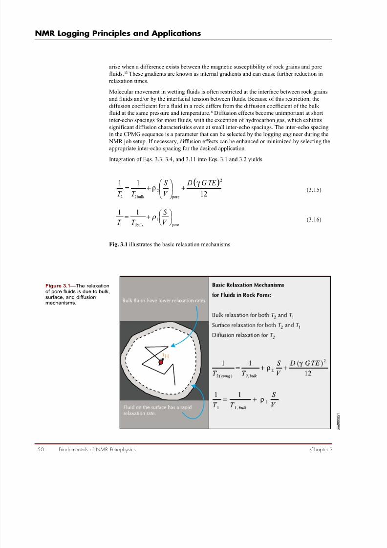
7/28/2019 NMR Logging Principles and Applications
http://slidepdf.com/reader/full/nmr-logging-principles-and-applications 68/253
NMR Logging Principles and Applications
50 Fundamentals of NMR Petrophysics Chapter 3
arise when a difference exists between the magnetic susceptibility of rock grains and pore
fluids.13 These gradients are known as internal gradients and can cause further reduction in
relaxation times.
Molecular movement in wetting fluids is often restricted at the interface between rock grains
and fluids and/or by the interfacial tension between fluids. Because of this restriction, the
diffusion coefficient for a fluid in a rock differs from the diffusion coefficient of the bulk
fluid at the same pressure and temperature.6 Diffusion effects become unimportant at short
inter-echo spacings for most fluids, with the exception of hydrocarbon gas, which exhibits
significant diffusion characteristics even at small inter-echo spacings. The inter-echo spacing
in the CPMG sequence is a parameter that can be selected by the logging engineer during the
NMR job setup. If necessary, diffusion effects can be enhanced or minimized by selecting the
appropriate inter-echo spacing for the desired application.
Integration of Eqs. 3.3, 3.4, and 3.11 into Eqs. 3.1 and 3.2 yields
( )12
112
pore2
bulk 22
TE G D
V
S
T T
γ
ρ +
+= (3.15)
pore
1
bulk 11
11
+=
V
S
T T ρ (3.16)
Fig. 3.1 illustrates the basic relaxation mechanisms.
Figure 3.1— The relaxationof pore fluids is due to bulk,
surface, and diffusion
mechanisms.
o m 0 0 0 8 5 1
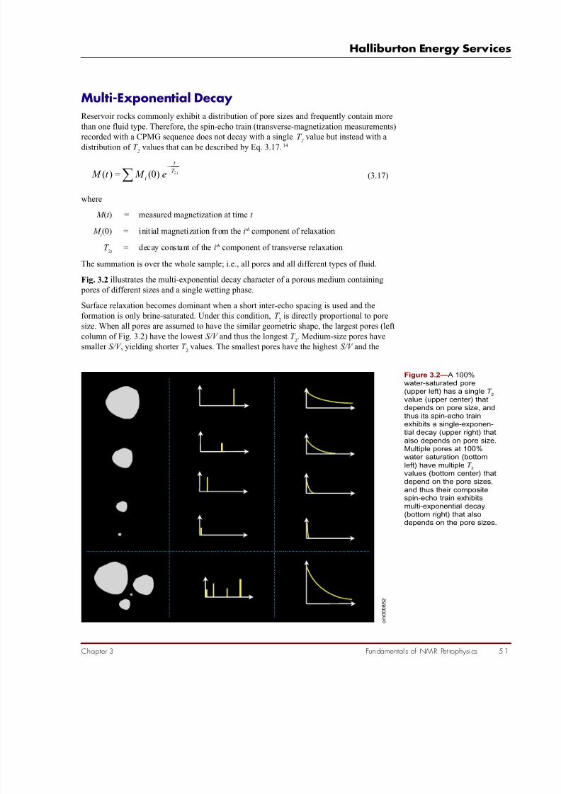
7/28/2019 NMR Logging Principles and Applications
http://slidepdf.com/reader/full/nmr-logging-principles-and-applications 69/253
Fundamentals of NMR Pet rophysics 51
Halliburton Energy Services
Chapter 3
Multi-Exponential Decay
Reservoir rocks commonly exhibit a distribution of pore sizes and frequently contain more
than one fluid type. Therefore, the spin-echo train (transverse-magnetization measurements)
recorded with a CPMG sequence does not decay with a single T 2 value but instead with adistribution of T
2values that can be described by Eq. 3.17.14
∑−
= iT
t
i e M t M 2)0()( (3.17)
where
M (t ) = measured magnetization at time t
M i(0) = initial magnetization from the ith component of relaxation
T 2i
= decay constant of the ith component of transverse relaxation
The summation is over the whole sample; i.e., all pores and all different types of fluid.
Fig. 3.2 illustrates the multi-exponential decay character of a porous medium containing pores of different sizes and a single wetting phase.
Surface relaxation becomes dominant when a short inter-echo spacing is used and the
formation is only brine-saturated. Under this condition, T 2
is directly proportional to pore
size. When all pores are assumed to have the similar geometric shape, the largest pores (left
column of Fig. 3.2) have the lowest S/V and thus the longest T 2. Medium-size pores have
smaller S/V , yielding shorter T 2
values. The smallest pores have the highest S/V and the
Figure 3.2— A 100%
water-saturated pore(upper left) has a single T
2
value (upper center) that
depends on pore size, and
thus its spin-echo trainexhibits a single-exponen-
tial decay (upper right) that
also depends on pore size.Multiple pores at 100%water saturation (bottom
left) have multiple T 2
values (bottom center) thatdepend on the pore sizes,
and thus their compositespin-echo train exhibitsmulti-exponential decay
(bottom right) that alsodepends on the pore sizes.
T 2
T 2
T 2
T 2Time
Time
Time
Time
Time
T 2
o m 0 0 0 8 5 2

7/28/2019 NMR Logging Principles and Applications
http://slidepdf.com/reader/full/nmr-logging-principles-and-applications 70/253
NMR Logging Principles and Applications
52 Fundamentals of NMR Petrophysics Chapter 3
shortest T 2
values. For a single pore, the magnetization decays exponentially, and the signal
amplitude is given by15
t V
S
e M t M
−
=
2
0)(
ρ
(3.18)
M 0
is proportional to the volume of fluid in the pore. When the complete distribution of the
100% water-saturated pores is considered (bottom left of Fig. 3.2), these pores exhibit a
distribution of T 2
values (bottom center of Fig. 3.2). The associated signal amplitude is the
sum of the signal amplitudes arising from the fluid in individual pores (bottom right of Fig
3.2), and the signal amplitude is given by
∑
−
=t
V
S
i
ie M t M 2
0)( ρ
(3.19)
where (S/V )iis the surface-to-volume ratio of the ith pore. Obviously,
∑=i M M 0)0( (3.20)
If M 100%
(0) (the measured magnetization for 100% bulk water with the same sensitive
volume) is known, then M (0) and M 0i
can be calibrated to porosity:
∑∑∑ ==== iii
M
M
M
M
M
M φφ
)0()0()0(
)0(
100%
0
100%
0
100%
(3.21)
where
φ = calibrated porosity of the formation
φi
= calibrated porosity associated with all pores of the ith pore size
(also known as the incremental porosity)
Therefore, the T 2
distribution (in the form of the amplitudes M 0i
associated with the time
constants T 2i) is calibrated to the porosity distribution (the individual pores φ
iwith the
associated time constants T 2i).
If the pores are partially saturated, i.e., the pores contain oil and/or gas in addition to water,
then the oil and gas contribute to the measured magnetization as follows:
gas2oil22
gasoil0)(
T
t
T
t t
V
S
ie M e M e M t M i
−−
−
++=∑ρ
(3.22)
where
M oil
= magnetization produced by oil protons in the pores
M gas = magnetization produced by gas protons in the pores
T 2oil
= T 2
of oil measured with a CPMG sequence
T 2gas
= T 2
of gas measured with a CPMG sequence
Eq. 3.22 assumes that the rock is water-wet and that the spin-echo decays of both oil and gas
can be characterized by using a single exponential expression which represents the bulk and
diffusion relaxation properties of the non-wetting fluids. Actually, many crude oils are

7/28/2019 NMR Logging Principles and Applications
http://slidepdf.com/reader/full/nmr-logging-principles-and-applications 71/253
Fundamentals of NMR Pet rophysics 53
Halliburton Energy Services
Chapter 3
composed of multiple hydrocarbon types and thus have complex decay spectra that must be
represented by multi-exponential sums. Furthermore, if oil or gas occupies part of a pore,
then the volume of water in the pore is reduced. Because the volume of water decreases while
the surface area of the pore remains the same, the ratio V/S decreases. Because the corre-
sponding T 2 of the pore water is proportional to V/S , it follows that V/S also decreases. Thus,when a non-wetting fluid is present, the T
2spectrum no longer represents a pore-size distribu-
tion because it contains a bulk response from the non-wetting fluid. Pores containing the non-
wetting fluid either appear in the spectrum at a decay time that is faster than is normally
associated with the pores, or do not appear at all if the surface layer is too thin. The porosity
in these pores is accounted for in the non-wetting bulk fluid response; thus, although the
distribution is distorted, the porosity is not affected.
Because, in practice, it is difficult to consider each pore individually, all pores with similar
surface-to-volume ratios and non-wetting fluids having similar T 2
values are grouped to-
gether. With this grouping, the sums in the magnetization equations have a manageable
number of terms.
Echo-Fit for T 2 DistributionOne of the most important steps in NMR data processing is to determine the T
2distribution
that produces the observed magnetization. This step, called echo-fit or mapping, is a math-
ematical inversion process. Fig. 3.3 illustrates the input (echo train) and output (T 2
distribu-
tion) of the mapping process. Eq. 3.23 displays the system of equations that represent the
individual echoes. Normally, the T 2
distribution of rocks is a continuous function. However,
to simplify fitting the echo train, the mapping process uses a multi-exponential model that
assumes that the T 2
distribution consists of m discrete relaxation times T 2i with corresponding
porosity components φi. The values of T
2iare pre-selected (for example, 0.5, 1, 2, 4, 8, 16,
32, 64, 128, 256, 512, 1024 ms … ), and the mapping process focuses on determining the
porosity components of each distribution.
noiseeeeenecho
noiseeeeeecho
noiseeeeeecho
m
m
m
T nt
m
T nt
T nt
T nt
T t
m
T t
T t
T t
T
t
m
T
t
T
t
T
t
++⋅⋅⋅+++=
++⋅⋅⋅+++=
++⋅⋅⋅+++=
−
−
−
−
−
−
−
−
−
−
−
−
,23,22,21,2
,23,22,21,2
,23,22,21,2
)()(
3
)(
2
)(
1
)2()2(
3
)2(
2
)2(
1
)1()1(
3
)1(
2
)1(
1
)(
)2(
)1(
φφφφ
φφφφ
φφφφ
.
.
.
(3.23)
where TE iit =)( and i = 1, … n, is the time when the ith echo was acquired.
Figure 3.3— Through echo
fitting, the echo train (echoamplitude as a function of time) is mapped to a T
2
distribution (porosity as a
function of T 2).
o m 0 0 1 2 6 4
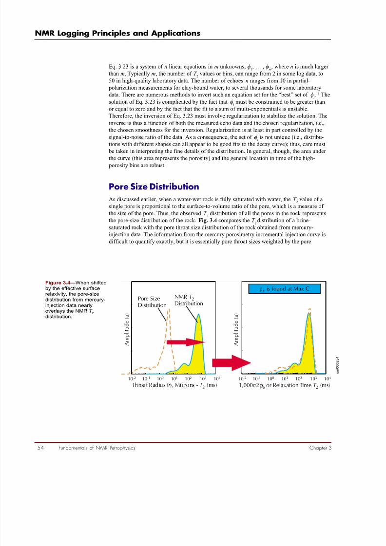
7/28/2019 NMR Logging Principles and Applications
http://slidepdf.com/reader/full/nmr-logging-principles-and-applications 72/253
NMR Logging Principles and Applications
54 Fundamentals of NMR Petrophysics Chapter 3
Eq. 3.23 is a system of n linear equations in m unknowns, φ1, … , φ
m, where n is much larger
than m. Typically m, the number of T 2
values or bins, can range from 2 in some log data, to
50 in high-quality laboratory data. The number of echoes n ranges from 10 in partial-
polarization measurements for clay-bound water, to several thousands for some laboratory
data. There are numerous methods to invert such an equation set for the “best” set of φi.16
Thesolution of Eq. 3.23 is complicated by the fact that φ
imust be constrained to be greater than
or equal to zero and by the fact that the fit to a sum of multi-exponentials is unstable.
Therefore, the inversion of Eq. 3.23 must involve regularization to stabilize the solution. The
inverse is thus a function of both the measured echo data and the chosen regularization, i.e.,
the chosen smoothness for the inversion. Regularization is at least in part controlled by the
signal-to-noise ratio of the data. As a consequence, the set of φiis not unique (i.e., distribu-
tions with different shapes can all appear to be good fits to the decay curve); thus, care must
be taken in interpreting the fine details of the distribution. In general, though, the area under
the curve (this area represents the porosity) and the general location in time of the high-
porosity bins are robust.
Pore Size DistributionAs discussed earlier, when a water-wet rock is fully saturated with water, the T
2value of a
single pore is proportional to the surface-to-volume ratio of the pore, which is a measure of
the size of the pore. Thus, the observed T 2
distribution of all the pores in the rock represents
the pore-size distribution of the rock. Fig. 3.4 compares the T 2distribution of a brine-
saturated rock with the pore throat size distribution of the rock obtained from mercury-
injection data. The information from the mercury porosimetry incremental injection curve is
difficult to quantify exactly, but it is essentially pore throat sizes weighted by the pore
NMRDistribution
T 2Pore SizeDistribution
A m p l i t u d e ( a )
A m p l i t u d e ( a )
10-2 10-210-1 10-1103 103104 104100 100101 101102 102
Throat Radius ( ), Microns - (ms)r T 2 1,000r/2 or Relaxation Time (ms)e 2T
ρe is found at Max C.
ρ
o m 0 0 0 8 5 4
Figure 3.4— When shifted
by the effective surfacerelaxivity, the pore-size
distribution from mercury-
injection data nearlyoverlays the NMR T
2
distribution.

7/28/2019 NMR Logging Principles and Applications
http://slidepdf.com/reader/full/nmr-logging-principles-and-applications 73/253
Fundamentals of NMR Pet rophysics 55
Halliburton Energy Services
Chapter 3
volumes to which the pore throats control access. As seen in the left of the figure, when a
shift is applied to account for factors such as surface relaxivity, the T 2
distribution shows a
remarkable correlation with the pore throat size distribution. Although distributions from
NMR and mercury can often be shifted to closely overlay each other, the distributions
represent somewhat different rock properties. This good quantitative agreement is due to thecorrelations often seen among some properties of sedimentary rocks.
Mappings such as Fig. 3.4 produce an effective relaxivity ( ρe). Effective relaxivity is intro-
duced to account for the fact that NMR responds to pore “body” size whereas mercury-
injection capillary pressure (MICP) is controlled mainly by the pore throat sizes. Thus, ρeis
proportional to the product of the intrinsic surface relaxivity ( ρ) and the ratio of pore throat
size to pore body size.17
Fig. 3.5 shows how relaxation-time distributions compare to MICP pore size distributions for
three types of lithologies. The relaxivity of sandstones is commonly greater than the
relaxivity of carbonates, which is the case for the sample data depicted in the figure.
The T 2
distribution from NMR data offers a reasonable estimate of a zone’s pore size
distribution when the zone is 100% water-saturated, as shown in Fig. 3.6 for sandstone and
carbonate samples. Even when hydrocarbons are present, BVI delineates fine-grained sandsfrom coarse-grained sands. This information is very helpful when evaluating reservoir quality
and depositional environment.
Figure 3.5— For a
particular rock, the T 2
distribution can becompared with the
mercury-injection pore-size
distribution to determinethe effective surface
relaxivity.
Pore throat distributionNMR distribution
Sandstone= 2.15 md
Porosity = 9.7 p.u.= 23.0 m/s
K air
e ρ µ
Dolomite= 7.41 md
Porosity = 15.8 p.u.= 5.35 m/s
K air
e ρ µ
Limestone= 12.3 md
Porosity = 10.5 p.u.= 3.16 m/s
K air
e ρ µ
10-1 103 10410-0 101 102
T 2 Relaxation Time, or 1,000/2 (ms)e ρ
A m p l i t u d e ( a )
o m 0 0 0 8 5 5

7/28/2019 NMR Logging Principles and Applications
http://slidepdf.com/reader/full/nmr-logging-principles-and-applications 74/253
NMR Logging Principles and Applications
56 Fundamentals of NMR Petrophysics Chapter 3
Figure 3.6— The correla-
tion between MCIP and T 2
distributions offers a
reasonable assurance that
the T 2
distributions estimate
a sensible pore sizedistribution when pores are
100% water-saturated.
Sandstone Samples
Carbonate Samples
o m 0 0 1 2 6 5
o m 0 0 1 2 6 6

7/28/2019 NMR Logging Principles and Applications
http://slidepdf.com/reader/full/nmr-logging-principles-and-applications 75/253
Fundamentals of NMR Pet rophysics 57
Halliburton Energy Services
Chapter 3
Determination of BVI
Estimating BVI , the bulk volume of irreducible water in a formation, is one of the earliest
and still one of the most widely used applications of NMR logging. Currently, two methods
are available for BVI determination. The first method, cutoff BVI (CBVI ), is based on a fixed T
2value (T
2cutoff ) that divides the T
2distribution into two components, one consisting of pore
sizes containing bound water and the other consisting of pore sizes containing free fluids.
The second method for BVI determination, called spectral BVI (SBVI ), is based on the
recognition that a given pore can contain both free and bound fluids.
In the NMR literature, the concept of bound water ( BVI ) is used in two different ways. The
first refers to the water contained in the pore space that will not flow out of the rock and into
the wellbore during production. This volume is accurately determined only by a relative
permeability measurement, but can be reasonably estimated from a capillary-pressure
saturation curve. This water volume is primarily a property of the rock and the wetting
conditions. The second use of BVI refers to the water that is not displaced by hydrocarbons
during the filling of the reservoir. This volume is a function of both the capillary-pressure
curve for the rock and the height above free water. In a transition zone, this water volume can
include water that can be produced. However, for a sufficient height above free water,capillary forces can drive water saturation to levels well below the point at which the relative
permeability to water is effectively zero. In many reservoirs, the transition zone occupies
only a small fraction of the hydrocarbon column, and the hydrocarbon column is short
enough that no significant difference exists between the two BVI values. If the two BVI values
do differ significantly, then it is important to decide whether BVI is being used to estimate
water production or to estimate permeability. For permeability estimation, especially when
drilling with oil-based mud, the BVI must be the volume of remaining water not displaced
by oil.
Cutoff BVI
Fig. 3.7 shows the CBVI concept. The NMR estimate of BVI is based on the assumption that
bound fluids reside in small pores and producible fluids reside in large pores. This assump-
tion is based on the fact that pore throat size and pore body size are often related. Because T 2
Figure 3.7— When a CBVI
model is used for NMR log
interpretation, a fixed T 2cutoff
is selected to calculate BVI .FFI
S p e c t r a l F r a c t i o n
0.8
1.0
0.9
0.7
0.6
0.5
0.4
0.3
0.2
0.1
BVI
CBVI T
Model:A Fixed 2cutoff
0.00.1 1.0 10 100 1,000
N o r m
a l i z e d I n c r e m e n t a l P o r o s i t y
Relaxation Time (ms)
0.8
1.0
0.9
0.7
0.6
0.5
0.4
0.3
0.2
0.1
0.0 o m 0 0 0 8 5 6

7/28/2019 NMR Logging Principles and Applications
http://slidepdf.com/reader/full/nmr-logging-principles-and-applications 76/253
NMR Logging Principles and Applications
58 Fundamentals of NMR Petrophysics Chapter 3
values can be related to pore body size, a T 2
value can be selected below which the corre-
sponding fluids are expected to reside in small pores and are thus immobile, and above which
the corresponding fluids are expected to reside in larger pores and thus can move freely. This
T 2
value is called the T 2
cutoff (T 2cutoff
). Through its partitioning of the T 2
distribution, the
T 2cutoff divides MPHI into two parts, BVI and FFI , as shown in Fig. 3.7. The BVI portion isreferred to as the cutoff BVI (CBVI ).18
Instead of assuming a relaxation-time cutoff, a T 2cutoff
can be determined in the laboratory with
NMR measurements on core samples. Core samples are analyzed for NMR characteristics at
two saturation conditions, S w
= 100% and (after establishing the appropriate value of satura-
tion from a capillary-pressure curve, or directly desaturating the sample to the appropriate
capillary pressure) S w
= irreducible. A centrifuge technique or a porous-plate technique at a
specified capillary pressure is used to achieve the latter condition. The T 2
distributions are
compared as illustrated in Fig. 3.8. The two T 2
distributions are displayed in two ways:
incremental porosity and cumulative porosity. (The cumulative porosity at a particular T 2, say
T 2,U
, is the integral of the incremental porosity for all T 2
values less than or equal to T 2,U
.) The
cumulative curves are used to determine T 2cutoff
. To determine T 2cutoff
from a plot of T 2
vs.
cumulative porosity, enter the plot from the cumulative porosity axis at the porosity at which
the sample is at irreducible condition. Project horizontally to the cumulative porosity curvefor S
w= 100%. Upon intersecting this curve, project down to the T
2axis. The T
2value of the
intersection of this projection with the T 2
axis is the T 2cutoff
.18
In the absence of laboratory data, default values based on lithology are used for T 2cutoff
. A
T 2cutoff
of 33 ms is used for sandstones and 92 ms for carbonates. These values work very well
in the Gulf of Mexico area. T 2cutoff
values, however, are affected not only by lithology, but also
by several other factors, such as pore-wall chemistry, minor paramagnetic or ferromagnetic
components, texture, pore throat to pore body ratios, and other factors not well understood.
Figure 3.8— NMR mea-surements on fullysaturated (S
w = 100%)
core samples and onsamples at irreduciblesaturation (S
wi ) can be
used to establish a T 2cutoff
for use in a CBVI model.
100% SaturatedCumulative
Incremental
After toC
Pc S umulative
Incremental
wi
2.5 25
2.0 20
1.5 15
1.0 10
0.5 5
0.1 1.0 10 100 1,000 10,000
I n c r e m e n t a l P o r o s i t y ,
%
C u m u l a t i v e P o r o s i t y ,
%
RelaxationTime ( ), msT 2
0.0 0
B
V I
F F I
M R I P o r o s i t y
T 2cutoff
o m 0 0 0 8 5 7

7/28/2019 NMR Logging Principles and Applications
http://slidepdf.com/reader/full/nmr-logging-principles-and-applications 77/253
Fundamentals of NMR Pet rophysics 59
Halliburton Energy Services
Chapter 3
Figure 3.9— In coresamples from an appar-ently homogeneous
reservoir, laboratory-derived T
2cutoff values can
vary. The red line repre-sents the average value of the cutoff.
T 2cutoff
1 10 1000
5
10
15
20
25
SampleNumber
o m 0 0 0 8 5 8
These factors can cause T 2cutoff
to vary among samples within a single lithology, as illustrated
in Fig. 3.9.Given the fact that T
2is directly proportional to pore size, a cutoff T
2represents a pore-size
cutoff or a capillary-pressure cutoff. Thus, T 2cutoff
values are a function of capillary pressure
along with the surface relaxivity. Laboratory examination of core samples to determine T 2cutoff
by the method illustrated in Fig. 3.8 is dependent on the capillary pressure chosen to create
the irreducible condition. This pressure depends on whether BVI is being used for producible
water or permeability. In the second case, it depends on the height above free water along
with the capillary-pressure curve of the rock.
Even though a T 2cutoff
may have been determined that best represents the irreducible saturation
condition of a particular rock type at the appropriate capillary pressure, this single relaxation
time may not properly represent the irreducible saturation condition of a different rock type.
One reason for this difference in T 2cutoff
values is the different capillary pressure at which
irreducible water condition is achieved in different rocks. This situation is illustrated in Fig.
3.10. In this figure, the capillary pressure appropriate for rock type A is too low for rock typeB. Thus, a cutoff value established for rock type B using this capillary pressure would
identify an overly high irreducible water saturation. Establishment of a T 2cutoff
using the
capillary pressure needed for rock type B may not give the same cutoff value found for rock
type A.
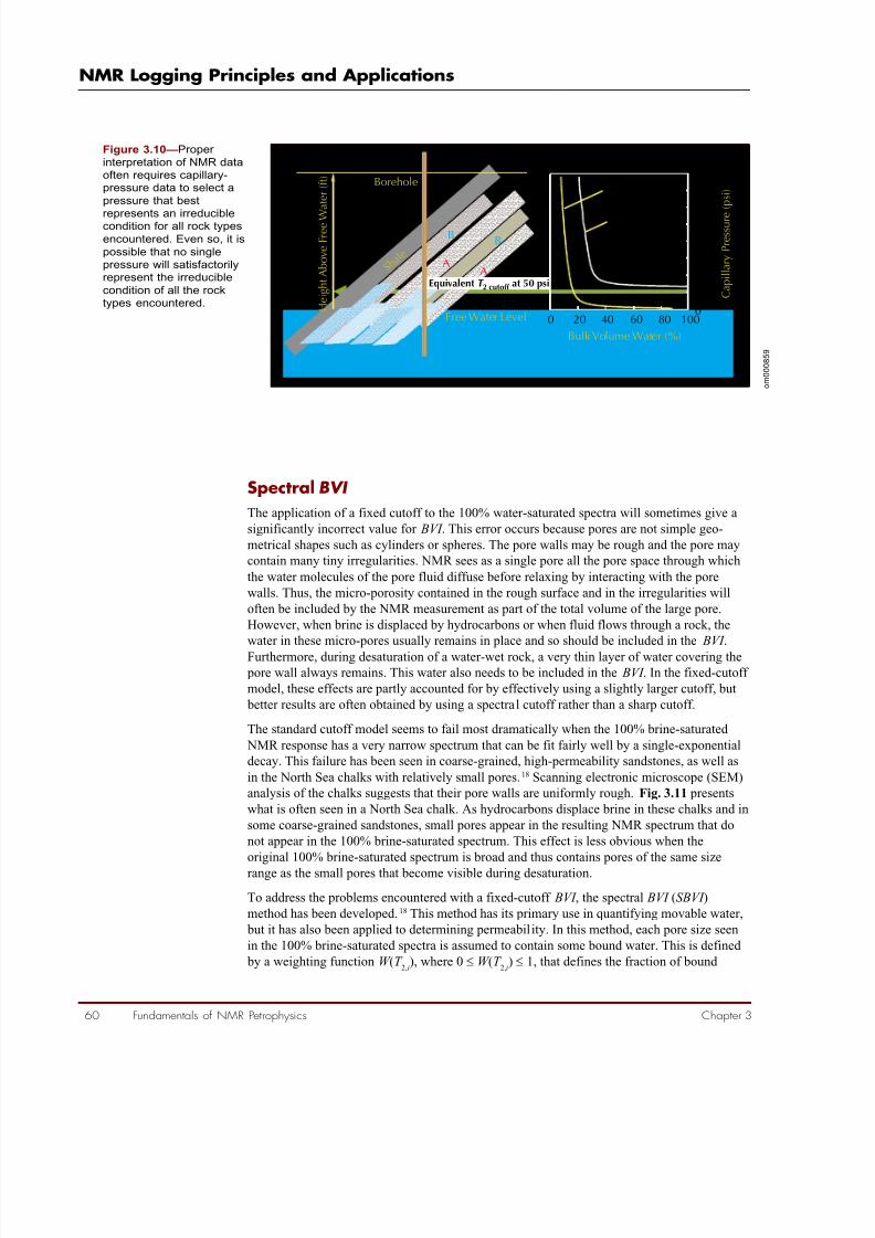
7/28/2019 NMR Logging Principles and Applications
http://slidepdf.com/reader/full/nmr-logging-principles-and-applications 78/253
NMR Logging Principles and Applications
60 Fundamentals of NMR Petrophysics Chapter 3
Spectral BVI
The application of a fixed cutoff to the 100% water-saturated spectra will sometimes give a
significantly incorrect value for BVI . This error occurs because pores are not simple geo-
metrical shapes such as cylinders or spheres. The pore walls may be rough and the pore may
contain many tiny irregularities. NMR sees as a single pore all the pore space through which
the water molecules of the pore fluid diffuse before relaxing by interacting with the pore
walls. Thus, the micro-porosity contained in the rough surface and in the irregularities will
often be included by the NMR measurement as part of the total volume of the large pore.
However, when brine is displaced by hydrocarbons or when fluid flows through a rock, the
water in these micro-pores usually remains in place and so should be included in the BVI .
Furthermore, during desaturation of a water-wet rock, a very thin layer of water covering the
pore wall always remains. This water also needs to be included in the BVI . In the fixed-cutoff
model, these effects are partly accounted for by effectively using a slightly larger cutoff, but
better results are often obtained by using a spectral cutoff rather than a sharp cutoff.
The standard cutoff model seems to fail most dramatically when the 100% brine-saturated
NMR response has a very narrow spectrum that can be fit fairly well by a single-exponential
decay. This failure has been seen in coarse-grained, high-permeability sandstones, as well as
in the North Sea chalks with relatively small pores.18 Scanning electronic microscope (SEM)
analysis of the chalks suggests that their pore walls are uniformly rough. Fig. 3.11 presents
what is often seen in a North Sea chalk. As hydrocarbons displace brine in these chalks and in
some coarse-grained sandstones, small pores appear in the resulting NMR spectrum that do
not appear in the 100% brine-saturated spectrum. This effect is less obvious when the
original 100% brine-saturated spectrum is broad and thus contains pores of the same size
range as the small pores that become visible during desaturation.
To address the problems encountered with a fixed-cutoff BVI , the spectral BVI (SBVI )
method has been developed.18 This method has its primary use in quantifying movable water,
but it has also been applied to determining permeability. In this method, each pore size seen
in the 100% brine-saturated spectra is assumed to contain some bound water. This is defined
by a weighting function W (T 2,i
), where 0 ≤ W (T 2,i
) ≤ 1, that defines the fraction of bound
Figure 3.10— Proper
interpretation of NMR dataoften requires capillary-pressure data to select a
pressure that best
represents an irreduciblecondition for all rock types
encountered. Even so, it is
possible that no singlepressure will satisfactorilyrepresent the irreducible
condition of all the rocktypes encountered. H
eightAboveFreeW
ater(ft)
CapillaryPressure
(psi)RockType A
RockType B
350
400
300
250
200
150
100
0
50
0 20 40 60 80 100Free Water Level
Borehole
BulkVolume Water (%)
S h a l
e
BB
AA
Equivalent at 50 psiT 2 cutoff
o m 0 0 0 8 5 9

7/28/2019 NMR Logging Principles and Applications
http://slidepdf.com/reader/full/nmr-logging-principles-and-applications 79/253
Fundamentals of NMR Pet rophysics 61
Halliburton Energy Services
Chapter 3
Figure 3.11— In a coarse-
grained rock that is fullywater-saturated (upper panel), the T
2distribution
will exhibit a single sharp
peak. No signal is ob-served below the T 2cutoff
value; hence, CBVI = 0.
After oil displaces most of the movable water in thesame rock (lower panel),
two peaks are found in theT
2distribution. One
appears below the T 2cutoff
value and is due toirreducible water on thepore surface. The other
appears above the T 2cutoff
value and is due to the oil.The T
2value of the second
peak is close to the T 2
of bulk oil. Hence, after most
of the water has beendisplaced, CBVI canbe calculated.
T 2
T 2
S w
< 100%
S w
= 100%
o m 0 0 0
8 6 0
Figure 3.12— For a givenT
2, the SBVI weighting
factor gives the fractional
volume of irreducible fluidsin the pores whose size isassociated with that T
2.
The model shown is a stepfunction and is commonly
used to describe theweighting factors.
FFI BVI
CBVI Model: Standard Cutoff
S p e c t r a l F r a c t i o n
Relaxation Time (ms)
0.8
1.0
0.9
0.7
0.60.5
0.4
0.3
0.2
0.1
0.00.1 1.0 10 100 1,000
N o r m a l i z e d I n c r e m e n t a l P o r o s i t y
0.8
1.0
0.9
0.7
0.60.5
0.4
0.3
0.2
0.1
0.0
SBVI Model:A Step Function
o m 0 0 0 8 6 1
water associated with each pore size, as shown in Fig. 3.12. Various methods have been
proposed in the literature to obtain the weighting functions.19, 20 One class of methods is based
on models in which the pores have a simple geometrical shape and in which the bound water
forms a thin film on the pore walls. These models give similar weighting functions for the
various simple pore shapes. However, the methods in this class all suffer from the simplistic
nature of the models.

7/28/2019 NMR Logging Principles and Applications
http://slidepdf.com/reader/full/nmr-logging-principles-and-applications 80/253
NMR Logging Principles and Applications
62 Fundamentals of NMR Petrophysics Chapter 3
Another class of models takes a more phenomenological approach. Comparison of formulas
for permeability, examination of thin-film models, study of experimental data, and general
considerations suggest a weighting function of the form
bmT W
i
i
+= ,21
(3.24)
T 2,i
is the T 2
relaxation time associated with the ith bin, and m and b are parameters that
depend on pore geometry and height above free water established from core capillary
desaturation measurements and NMR measurements on the partially saturated cores. Then
ii
n
i
W SBVI φΣ=
=1
(3.25)
where n is the number of bins and φi is the porosity associated with each bin.
Fig. 3.13 provides a motivation for Eq. 3.24. For a set of core samples, the figure shows a
linear relationship between 1/S wirr and T 2 gm, where S wirr is the water saturation at a givencapillary pressure, and T 2 gm
is the geometric mean of the relaxation spectra. The functional
form for the weight function makes sense in the limits of small and large pores.
In almost any reasonable pore model, the percentage of bound water in a pore decreases as
pore size increases. In its simplest functional form, this property is expressed as
Figure 3.13— Thisexample comparing core-measured irreducible
water saturation (1/S wirr ) tothe geometric mean (T
2gm)
of core T 2
spectra illus-
trates that a linear relationship exists betweenrelaxation time and 1/S
wirr .
7
8
6
5
2
4
3
10 20 40 60 80 100 120 140
1 /
( C o r e
)
S w
i r r
1/ = +S T b wirr core 2
T 2gm’ ms
o m 0 0 0 8 6 2

7/28/2019 NMR Logging Principles and Applications
http://slidepdf.com/reader/full/nmr-logging-principles-and-applications 81/253
Fundamentals of NMR Pet rophysics 63
Halliburton Energy Services
Chapter 3
i
i
T W
,2~1
(3.26)
For small pores, a pore size exists below which W i
must be equal to 1. Thus, for all T 2
values
above a certain small T 2, a constant term b must be added to the right side of the simple
relationship given by Eq. 3.26. Taking b = 1 implies every pore has some movable water, but
this implication is never correct at a given height above free water.
In general, for a particular value of m and b, a value k exists such that W k
will be 1 for the
time bin T 2,k
. Then for all T 2,i
less than T 2,k
, W iis assumed to be 1. Although the best method
for establishing m and b is measurements on cores from the zone being logged, work by
Coates et al.18 on a set of 340 sandstone and 71 carbonate samples has established generic
values. In this work, b was taken as 1, and the value of m for sandstones and limestones was
found to be 0.0618/ms and 0.0113/ms, respectively.
Models with b = 1 are most prone to error when there is a significant porosity in small pores
(such as in clay pores) that must be weighted as one.
A method to determine m and b from laboratory measurements on s core samples is to solve
the set of equations 3.27.
n sn s s s swirr
nnwirr
nnwirr
W W W S
W W W S
W W W S
,2,21,1,
,22,221,2122,
,12,121,1111,
φφφφ
φφφφ
φφφφ
+++=
+++=
+++= ⋅⋅⋅
⋅⋅⋅
⋅⋅⋅
.
.
.
(3.27)
W i, i = 1, … , n, are the weighting functions. S
wirr,i , i = 1, …, s, are the water saturations of the
samples at a chosen capillary pressure. φi, i = 1, …, s, are the porosities of the samples.
φi,j , j = 1, …, n, are the components of the porosity of the i
th
sample in j
th
bin of the m-termexponential fit to the NMR decay curve. Eq. 3.25 can also be solved for other forms of the
weighting function.
In general, for a 100% water-saturated rock, determining SBVI with a correct set of weighting
functions is a superior method of obtaining bound water from NMR measurements.
Application of the SBVI method becomes more complicated when the pores contain hydro-
carbons and water. If the rock is water-wet, two major effects must be considered. First,
because the weighting functions are non-zero over a wide range of relaxation times, hydro-
carbons will more likely be counted as bound water, driving SBVI to be too large. Second,
although the small pores that appear in the NMR spectra when hydrocarbons fill the center of
the pore body should be counted as 100% filled with bound water, the model may associate
them with weightings less than one, making SBVI too small. This effect is particularly
important when a sensitive zone of the logging tool is at irreducible water saturation. Count-
ing bound water as free water can only happen when a weighting function is used that isinappropriate for the rock type or for the height above free water. Currently, the suggested
best practice for determining BVI is to compute two bound-water values—one from the fixed-
cutoff and one from the SBVI method—and take the larger of the two. It should be noted that
this practice is strongly dependent on the weighting function used and is based on studies that
used functions for which b = 1.

7/28/2019 NMR Logging Principles and Applications
http://slidepdf.com/reader/full/nmr-logging-principles-and-applications 82/253
NMR Logging Principles and Applications
64 Fundamentals of NMR Petrophysics Chapter 3
MRIL Permeability Model
The NMR estimate of permeability is based on a combination of experimental and theoreti-
cal models and relationships.14 When all other factors are kept constant in these models and
relationships, permeability increases as connected porosity increases. The unit of permeabil-ity, the Darcy, has dimensions of area, and from practical considerations in petrophysical
applications, permeability can be considered as being proportional to the square of some
geometrical size. The correlation between capillary pressure curves and permeability strongly
support that the pertinent size is that of the pore throat.21, 22 NMR measures pore body size,
but in almost all sandstones and some carbonates, a strong correlation exists between pore
body size and pore throat size.
The two most commonly used expressions for permeability both vary as φ 4. This power of φ
is somewhat arbitrary but is loosely derived from Archie’s Law, the relationship of permeabil-
ity to resistivity, and with an additional factor to account for NMR measuring pore body size
not pore throat size. In one expression, the Free Fluid (or Coates) model, the size parameter
enters implicitly through T 2cutoff
, which determines the ratio of FFI to BVI , where FFI is the
free fluid volume and FFI = φ - BVI . In the other expression, the Mean T 2
(or SDR) model,
the size parameter enters through the geometrical mean of the relaxation spectra, T 2 gm.4
Theuse of these particular size parameters in the respective expressions is based on empirical
considerations. Other size measures have also been used. Fig. 3.14 illustrates both models.
Both models correlate very well to permeability from laboratory data on 100% brine-
saturated samples. The Mean T 2
model, however, fails when the pore contains hydrocarbons
because then T 2 gm
is not controlled exclusively by pore size.
The Free Fluid Model
In the Free Fluid (or Coates) model in its simplest form the permeability k is given by
22
=
BVI
FFI
C k
φ(3.28)
MPHI (MRIL porosity, which is discussed in the next section) is usually used for φ, and BVI
is obtained through the CBVI or SBVI method.18 The coefficient C is a variable that is
dependent on the processes that created the formation and can be different for each formation.
Experience has shown that the Coates model is more flexible than the Mean T 2
model.
Through careful core calibration, the Coates model has been customized for successful use in
different formations and reservoirs. As long as BVI does not include any hydrocarbon
contribution, BVI is not affected by an additional liquid phase such as oil or oil filtrates,
which is very important when analyzing hydrocarbon-bearing formations.
In unflushed gas zones, the MPHI used for porosity in the Coates formula may be too low
because of the low hydrogen index in such zones. Thus, MPHI must be corrected, or an
alternative porosity source should be used. Zones that maintain high residual gas saturation at
sufficient reservoir pressure will have SBVI and CBVI values that are too high and thus, to asmall degree, will yield permeability values that are too low. Heavier oils, which normally
have very short T 2
values, may be counted as BVI , thus causing permeability to be
underestimated.

7/28/2019 NMR Logging Principles and Applications
http://slidepdf.com/reader/full/nmr-logging-principles-and-applications 83/253
Fundamentals of NMR Pet rophysics 65
Halliburton Energy Services
Chapter 3
The Mean T 2Model
The Mean T 2
(or SDR) model is given by
422 φ gmT ak = (3.29)
In Eq. 3.29, NMR effective porosity is substituted for φ. As before, T 2 gm
is the geometric
mean of the T 2
distribution. As with the Coates model, the value a is a coefficient that
depends on the formation type.
Experience has shown that the Mean T 2
model works very well in zones containing only
water. However, if oils or oil filtrates are present, the mean T 2 is skewed toward the bulk-liquid T
2, and permeability estimates are erroneous. In unflushed gas zones, mean T
2values
are too low relative to the flushed gas zone, and permeability is consequently underestimated.
Because hydrocarbon effects on T 2 gm
are not correctable, the Mean T 2
model fails for hydro-
carbon-bearing formations.
In fractured formations, permeability estimates from both the Coates and SDR models are too
low because these models can only represent matrix permeability.
MRIL Porosity Model
The initial amplitude of the NMR spin-echo train, or the area under the T 2
distribution curve,
is proportional to the number of hydrogen protons that are contained in the pore fluids within
the sensitive volume. Thus, this amplitude can be calibrated to give a porosity value. Fig.3.15 shows the NMR porosity model for a water-wet formation. The upper part of the figure
is a typical volumetric model of the virgin zone, which consists of matrix and dry clay, clay-
bound water, capillary-bound water, movable water, oil, and gas. The middle part of the
Figure 3.14— The Coatespermeability model (top)
uses the FFI /BVI ratio todescribe changes in thesurface-to-volume ratio.
The SDR permeabilitymodel (bottom) uses anaverage T
2value to
describe changes in
surface-to-volume ratio.
Coates Model
BVI FFI
SDR Model
T 2cutoff T 2
T 2gm
T 2 o m 0
0 0 8 6 3

7/28/2019 NMR Logging Principles and Applications
http://slidepdf.com/reader/full/nmr-logging-principles-and-applications 84/253
NMR Logging Principles and Applications
66 Fundamentals of NMR Petrophysics Chapter 3
figure is the corresponding volumetric model for the invaded zone, which is the region in
which MRIL measurements are made; all model elements remain the same as in the virgin
zone except that the mud filtrate now displaces some of the movable water, oil, and gas. The
bottom part of the figure illustrates the MRIL response to porosity elements. Note that
MFFI refers to the same quantity as FFI , and MPHI does not include the contribution from
some of the water that is associated with clay porosity and perhaps other materials with
clay-size pores.
Fig 3.15 shows sharp divisions between the porosity elements associated with MFFI , BVI ,
and MCBW . These sharp divisions in porosity elements do necessarily correspond to sharp
divisions in the T 2
spectra. For BVI , this has already been discussed in detail. In the case of
clays, the water associated with clays has a range of decay times that can overlap decay times
for capillary-bound water; thus, a sharp division may not exist between MCBW and BVI in
the T 2 spectra.
Both matrix minerals and dry clay can contain hydrogen atoms in the form of hydroxyl
groups (OH). Because the T 1
relaxation times of these nuclei are too long to be polarized by a
moving MRIL tool, and their T 2
relaxation times are too short to be recorded, hydrogen in
OH groups and in water of hydration is invisible to the MRIL tool.23 The hydrogen nuclei of
clay-bound water are adsorbed on the surfaces of clay grains. These hydrogen protons in
clay-bound water can be polarized by the MRIL tool and can be recorded as long as a
sufficiently short TE is used. The clay-bound water is measured by an MRIL CPMG se-
quence with TE = 0.6 ms and with polarization time TW set for partial or full recovery. The
measurement yields the component of porosity referred to as MCBW , which provides an
estimate of clay-bound water. Similarly, hydrogen protons exist in capillary-bound water and
movable fluids, such as movable water, mud filtrates, oil, and gas. These hydrogen protons
are measured using a standard T 2-logging CPMG sequence with TE = 1.2 ms and with TW set
for full polarization. This measurement yields MPHI .
The measured echo-train amplitude, and thus MPHI , is affected by the hydrogen index HI of
the fluids. MPHI is calibrated to the number of protons in water having a hydrogen index of
1. If the hydrogen index of any of the fluids in the pore space is significantly different from 1,
then a correction to MPHI is required.
Figure 3.15— MRIL toolsrespond to the flushed-
zone (bottom volumetricmodel), in which mudfiltrate has displaced some
of the free fluids that werepresent in the virgin zone(top volumetric model).MRIL responses (bottom)
are sensitive to fluids butnot to matrix materials anddry clay. MRIL porosity is
affected by hydrogen index(HI ), polarization time(TW ), and inter-echospacing (TE ).
o m 0 0 0 8 6 4
Matrix and Dry ClayClay-boundWater
Capillary-boundWater
MovableWater
Oil Gas
Clay-boundWater
Capillary-boundWater
MovableWater
Oil GasMud Filtrate
MCBW MPHI
MSIG
MFFI BVI
Volumetric Model of the Virgin Zone
MRIL Porosity Response
Volumetric Model of the Invaded Zone
Matrix and Dry Clay

7/28/2019 NMR Logging Principles and Applications
http://slidepdf.com/reader/full/nmr-logging-principles-and-applications 85/253
Fundamentals of NMR Pet rophysics 67
Halliburton Energy Services
Chapter 3
Both MPHI and MCBW are affected by the polarization time TW . Both light oil and gas have
very long T 1
relaxation times. If the polarization time is too short, then MPHI may underesti-
mate effective porosity.
Both MPHI and MCBW are affected by inter-echo spacing TE . As TE decreases, faster T 2relaxation components can be detected. Conversely, increasing TE causes the loss of fast T
2
components, which in turn causes MPHI and MCBW to be too low.
In addition, MPHI and MCBW measurements are both affected by the 90° B1
pulse in their
CPMG sequences. If the pulse angles are less than 90°, the magnetization will be under-
tipped, the measured amplitude thus will be too small, and both MPHI and MCBW will be
underestimated. If their pulse angles are greater than 90°, then the magnetization will be
over-tipped, the measured amplitude will once more be too small, and both MPHI and
MCBW will be underestimated again. Calibration usually solves this problem.
References
1. Cowan, B., 1997, Nuclear Magnetic Resonance and Relaxation, Cambridge, Cambridge
University Press, Cambridge, U.K., p. 207–234.
2. Guimaraes, A.P., 1998, Magnetism and Magnetic Resonance in Solids, New York, John
Wiley & Sons, Inc., New York, p. 203–225.
3. Bendel, P., 1990, Spin-echo attenuation by diffusion in non-uniform field gradients,
Journal of Magnetic Resonance, v. 86, p. 509–515.
4. Kenyon, W.E., 1992, Nuclear magnetic resonance as a petrophysical measurement,
Nuclear Geophysics, v. 6, no. 2, p. 153–171. Later revised and published in 1997 as
Petrophysical principles of applications of NMR logging, The Log Analyst, v. 38, no. 2,
p. 21–43.
5. Vinegar, H., 1995, Relaxation mechanisms, chapter 3, in Georgi, D.T., ed., 36th Annual
SPWLA Logging Symposium: Nuclear magnetic resonance logging short course notes ,
variously paginated.
6. Prammer, M.G., et al., 1995, Lithology-independent gas detection by gradient-NMR
logging, SPE 30562, 1999 SPE Annual Technical Conference and Exhibition Proceed-
ings, v.Ω (Formation evaluation and reservoir geology), p. 325–336.
7. Zhang, Q., et al., 1998, Some exceptions to default NMR rock and fluid properties,
SPWLA 39th Annual Logging Symposium Transactions.
8. Brownstein, K.R., and Tarr, C.E., 1979, Importance of classical diffusion in NMR
studies of water in biological cells, Physical Review, Series A, v. 19, p. 2446–2453.
9. Kleinberg, R.L., Kenyon, W.E., and Mitra, P.P., 1994, Mechanism of NMR relaxation of
fluids in rock, Journal of Magnetic Resonance, Series A, v. 108, no. 2, p. 206–214.
10. Chang, D., et al., 1994, Effective porosity, producible fluid and permeability in carbon-
ates from NMR logging, paper A, 35th Annual SPWLA Logging Symposium Transac-tions, 21 p. Later published in 1997 in The Log Analyst, v. 38, no. 2, p. 60–72.
11. Chen, R., et al., 1994, Effects of hydrostatic pressure on proton and deuteron magnetic
resonance of water in natural rock and artificial porous media, Journal of Magnetic
Resonance, Series A, v. 110, p. 77–81.
7/28/2019 NMR Logging Principles and Applications
http://slidepdf.com/reader/full/nmr-logging-principles-and-applications 86/253
NMR Logging Principles and Applications
68 Fundamentals of NMR Petrophysics Chapter 3
12. Mardon, D., Prammer, M.G., and Coates, G.R., 1996, Characterization of light hydrocar-
bon reservoirs by gradient-NMR well logging, Magnetic Resonance Imaging , v. 14,
no. 7/8, p. 769–777.
13. Appel, M., Freeman, J.J., Perkins, R.B., Hofman, J.P., 1999, Restricted diffusion and
internal field gradients paper, SPWLA 40th Annual Logging Symposium Transactions.
14. Kenyon, W.E., et al., 1986, Compact and consistent representation of rock NMR data
from permeability estimation, SPE 15643, 1986 SPE Annual Technical Conference and
Exhibition preprint, 22 p. Later published in 1988 as a three-part study of NMR longitu-
dinal relaxation properties of water-saturated sandstones, SPE Formation Evaluation,
v. 3, no. 3, p. 622–636.
15. Kenyon, W.E., et al., 1989, Pore-size distribution and NMR in microporous cherty
sandstones, paper LL, in, 30th Annual SPWLA Logging Symposium Transactions, 24 p.
16. Golub, G.H., and Van Loan, C.F., 1983, Matrix computation, The Johns Hopkins Univer-
sity Press.
17. Marschall, D., Gardner, J.S., Mardon, D., and Coates, G.R., 1995, Method for correlating
NMR relaxometry and mercury injection data, SCA 9511 International SCA Symposium proceedings: SPWLA Society of Core Analysts Chapter-at-Large, 12 p.
18. Coates, G., et al., 1997, A new characterization of bulk-volume irreducible using mag-
netic resonance, paper QQ, 38th Annual SPWLA Logging Symposium Transactions, 14
p. Also published in 1997 in DiaLog , London Petrophysical Society, v. 5, no. 6, p. 9–16.
19. Chen, S., et al., 1998, Methods for computing Swi and BVI from NMR logs, HI , 39th
SPWLA Annual Logging Symposium.
20. Kleinberg, R.L., and Boyd, A., 1997, Tapered cutoffs for magnetic resonance bound
water volume, SPE 38737, 1997 SPE Annual Technical Conference and Exhibition
Proceedings, v.Ω (Formation evaluation and reservoir geology), part 2, p. 197–202.
21. Pittman, E.D., 1992, Relationship of porosity and permeability to various parameters
derived from mercury injection-capillary pressure curves for sandstone, AAPG Bulletin,
v. 76, no. 2, p. 191–198.
22. Thompson, A., Katz, A.J., and Krohn, C.E., 1987, The micro-geometry and transport
properties of sedimentary rock, Advances in Physics, v. 36, p. 625–694.
23. Prammer, M.G., et al., 1996, Measurements of clay-bound water and total porosity by
magnetic resonance logging, SPE 36522, 1996 SPE Annual Technical Conference and
Exhibition Proceedings, v.Ω (Formation evaluation and reservoir geology), p. 111–118.
Also published in 1996 in The Log Analyst, v. 37, no. 5, p. 61–69.
More discussion on fluid properties and NMR petrophysics can be found in the
following literature:
Ahmed, U., Crary, S.F., and Coates, G.R., 1989, Permeability estimation; the various sources
and their interrelationship, SPE 19604, SPE Annual Technical Conference and Exhibition
Proceedings, v.Ω (Formation evaluation and reservoir geology), p. 649-662. Later published in 1990 as The interrelationship between various permeability measurements,
1990 SPWLA International Well Logging Symposium Transactions, Beijing Chapter , 21
p. Later published in 1991 in Journal of Petroleum Technology, v. 43, no. 5, p. 578–587.
Later reprinted in 1994 in Petrophysics, SPE Reprint Series No. 39, p. 118–127.

7/28/2019 NMR Logging Principles and Applications
http://slidepdf.com/reader/full/nmr-logging-principles-and-applications 87/253
Fundamentals of NMR Pet rophysics 69
Halliburton Energy Services
Chapter 3
Allen, D., et al., 1988, Probing for permeability—An introduction of measurements, The
Technical Review, v. 36, no. 1, p. 6–20.
Baldwin, B.A., 1993, Immobile water determination in shaly sandstone, SCA 9314, in Annual
technical conference proceedings: Society of Professional Well Log Analysts, Society of
Core Analysts Chapter-at-Large, 14 p. Later published in 1994 in The Log Analyst , v. 35,
no. 3, p. 31–37.
Banavar, J.R., and Schwartz, L.M., 1987, Magnetic resonance as a probe of permeability in
porous media, Physical Review Letters, v. 58, no. 14, p. 1411–1414.
Banavar, J.R., and Schwartz,L.M., 1989, Probing porous media with nuclear magnetic
resonance, in Klafter, J., and Drake, J.M., eds., Molecular dynamics in restricted geom-
etries, Wiley, New York, p. 273–310.
Basan, P., et al., 1994, Variations in NMR relaxivity and its relationship to pore size in
sandstones from the South Morecambe Field, Irish Sea, paper AA, 16th SPWLA Euro-
pean Formation Evaluation Symposium Transactions, Aberdeen Chapter , 39 p.
Bergman, D.J., and Dunn, K.J., 1994, Theory of diffusion in a porous medium with applica-
tions to pulsed-field-gradient NMR, Physical Review, Series B, v. 50, p. 9153.
Bergman, D.J., and Dunn, K.J., 1995, NMR of diffusing atoms in a periodic porous medium
in the presence of a nonuniform magnetic field, Physical Review, Series E, v. 52,
no. 6, p. 6516.
Bergman, D.J., Dunn, K.J., and LaTorraca, G.A., 1995, Magnetic susceptibility contrast
and fixed field gradient effects on the spin-echo amplitude in a periodic porous medium
diffusion, Bulletin of the American Physical Society, v. 40, p. 695.
Blackband, S., et al., 1984, Discrimination of crude oil and water in sand and in bore cores
using NMR imaging, SPE 13401: Society of Petroleum Engineers, 17 p. Later published
in 1986 in SPE Formation Evaluation, v. 1, no. 1, p. 31–34.
Bobroff, S., et al., 1996, Quantitative porosity profiles and wettability contrast visualization
in sandstone by CPMG imaging, Magnetic Resonance Imaging , v. 14, no. 7/8, p. 907–
909.
Borgia, G.C., et al., 1990, Specific surface and fluid transport in sandstones through NMR
studies, SPE 20921, 1990 SPE European petroleum conference [Europec 90] Proceed-
ings. Later published in 1992 in SPE Formation Evaluation, v. 7, no. 3, p. 206–210.
Borgia, G.C., et al., 1996, Developments in core analysis by NMR measurements,
Magnetic Resonance Imaging , v. 14, no. 7/8, p. 751–760.
Borgia, G.C., et al., 1991, Proceedings of the first international conference on recent ad-
vances in NMR applications to porous media, Magnetic Resonance Imaging , v. 9, no. 5,
p. 639–888.
Borgia, G.C., et al., editors, 1994, Proceedings of the second international meeting on recent
advances in MR applications to porous media, Magnetic Resonance Imaging , v. 12, no. 2.
Borgia, G., Brancolini, A., Brown, R.J.S., Fantazzini, P., and Ragazzini, G., 1994, Water-air
saturation changes in restricted geometries studied by proton relaxation, Magnetic
Resonance Imaging, v. 12, p. 191–195.
7/28/2019 NMR Logging Principles and Applications
http://slidepdf.com/reader/full/nmr-logging-principles-and-applications 88/253
NMR Logging Principles and Applications
70 Fundamentals of NMR Petrophysics Chapter 3
Borgia, G.C., et al., 1994, Capillary water determination in core plugs; a combined study
based on imaging techniques and relaxation analysis, Magnetic Resonance Imaging ,
v. 12, no. 2, p. 221–224.
Borgia, G.C., et al., 1990, Specific surface and fluid transport in sandstones through NMR
studies, SPE 20921, 1990 SPE European petroleum conference [Europec 90] Proceed-
ings. Later published in 1992 in SPE Formation Evaluation, v. 7, no. 3, p. 206–210.
Borgia, G.C., Brown, R.J.S., and Fantazzini, P., 1995, The effect of diffusion and susceptibil-
ity differences on T 2
measurements for fluids in porous media and biological tissues,
Magnetic Resonance Imaging , v. 14, no. 7/8, p. 731–736.
Borgia, G.C., Brown, R.J.S., and Fantazzini, P., 1995, Scaling of spin-echo amplitudes with
frequency, diffusion coefficient, pore size and susceptibility difference for the NMR of
fluids in porous media and biological tissues, Physical Review, Series E, v. 51, p. 2104.
Bowers, M.C., et al., 1993, Determination of porosity types from NMR data and their
relationship to porosity types derived from thin section, SPE 26307, unsolicited paper,
45 p. Later published in 1995 in Journal of Petroleum Science and Engineering , v. 13,
p. 1–14.
Brown, R. J. S., 1961, Proton Relaxation in Crude Oils, Nature, v. 189, no. 4762, 387–388.
Brownstein, K.R., and Tarr, C.E., 1977, Spin-lattice relaxation in a system governed by
diffusion, Journal of Magnetic Resonance, v. 26, p. 17–24.
Carr, M.B., et al., 1996, Correlation of porosity types derived from NMR data and thin
section image analysis in a carbonate reservoir, Journal of Petroleum Science and
Engineering , v. 14, p. 115–131.
Chen, Q., Wang, W., and Cai, X., 1996, Application of NMR imaging to steam foam flooding
in porous media, Magnetic Resonance Imaging , v. 14, no. 7/8, p. 949–950.
Chen, S., and Georgi, D.T., 1997, Improving the accuracy of NMR relaxation distribution
analysis in clay-rich reservoirs and core samples, SCA 9702, in 1997 international
symposium proceedings: Society of Professional Well Log Analysts, Society of Core
Analysts Chapter-at-Large, 10 p.
Chen, S., et al., 1992, Quantitative NMR imaging of multiphase flow in porous media,
Magnetic Resonance Imaging , v. 10, p. 815–826.
Chen, S., Liaw, H.K., and Watson, A.T., 1993, Fluid saturation-dependent nuclear magnetic
resonance spin-lattice relaxation in porous media and pore structure analysis, Journal of
Applied Physics, v. 74, no. 3, p. 1473–1479.
Chen, S., Liaw, H.-K., and Watson, A.T., 1994, Measurements and analysis of fluid satura-
tion-dependent NMR relaxation and linebroadening in porous media, Magnetic Reso-
nance Imaging , v. 12, no. 2, p. 201–202.
Chen, S., et al., 1993, Characterization of rock pore structures using NMR restricted diffu-
sion measurements and analyses, SCA 9313, in Annual technical conference proceedings:
Society of Professional Well Log Analysts, Society of Core Analysts Chapter-at-Large,15 p.
Chen, S., et al., 1992, NMR imaging of multiphase flow in porous media, SPE 24760, 1992
SPE Annual Technical Conference and Exhibition Proceedings, v.Ω (Formation evalua-
tion and reservoir geology), p. 1013–1026. Also published in 1993: AIChE Journal
(American Institute of Chemical Engineers), v. 39, no. 6, p. 925–934.

7/28/2019 NMR Logging Principles and Applications
http://slidepdf.com/reader/full/nmr-logging-principles-and-applications 89/253
Fundamentals of NMR Pet rophysics 71
Halliburton Energy Services
Chapter 3
Chen, S., Qin, F., and Watson, A.T., 1994, Determination of fluid saturations during
multiphase flow experiments using NMR imaging techniques, AIChE Journal , v. 40,
p. 1238–1245.
Chen, S., et al., 1994, Characterization of fractures and multiphase flow in fractured perme-
able rocks using NMR imaging techniques, SCA 9402, in SCA international symposium
proceedings: Society of Professional Well Log Analysts, Society of Core Analysts,
Chapter-at-Large, p. 17–28. Also published in 1994 as, NMRI characterization of
fractures and multiphase transport in fractured porous media, SPE 28369, 1994 SPE An-
nual Technical Conference and Exhibition Proceedings, v.Ω (Formation evaluation and
reservoir geology), p. 65–79.
Chen, S., Ostroff, G., Georgi, D., 1998, Improving estimation of NMR log T2cutoff
value with
core NMR and capillary pressure measurements, SCA 9822.
Coates, G., et al., 1997, A new characterization of bulk-volume irreducible using magnetic
resonance, paper QQ, 38th Annual SPWLA Logging Symposium Transactions, 14 p. Also
published in 1997 in DiaLog (London Petrophysical Society), v. 5, no. 6, p. 9–16.
Coates, G. R., et al., 1993, Restrictive diffusion from uniform gradient NMR Well Logging,
SPE 26472.
Curwen, D.W., and Molaro, C., 1995, Permeability from magnetic resonance imaging logs,
paper GG, in 36th Annual SPWLA Logging Symposium Transactions, 12 p.
Davies, S., et al., 1990, Pore-size distributions from NMR spin-lattice relaxation measure-
ments of fluid saturated porous solids, part 2, Application to reservoir core samples,
Journal of Applied Physics, v. 67, no. 6, p. 3171–3176.
Davies, S., and Packer, K.J., 1990, Pore-size distributions from NMR spin-lattice relaxation
measurements of fluid-saturated porous solids, part 1, Theory and simulation, Journal of
Applied Physics, v. 67, p. 3163–3170.
Dodge, W.S., Shafer, J., and Klimentidis, R., 1996, Capillary pressure—the key to producible
porosity, paper J, in 37th Annual SPWLA Logging Symposium Transactions,13 p.
D’Orazio, F., et al., 1989, Application of nuclear magnetic resonance pore structure analysis
to porous silica, Journal of Applied Physics, v. 65, p. 742–751.
Dawson, R., Khoury, F., and Kobayashi, R., 1970, Self-Diffusion Measurements in Methane
by Pulsed Nuclear Magnetic Resonance, AIChEJ , Vol. 16, No. 5, 725–729.
Dunn, K-J., et al., 1994, On the calculation and interpretation of NMR relaxation time
distributions, SPE 28367, 1994 SPE Annual Technical Conference and Exhibition
Proceedings, v.Ω (Formation evaluation and reservoir geology), p. 45–54.
Foley, I., Farooqui, S. A., and Kleinberg, R. L., 1996, Effect of paramagnetic ions on NMR
relaxation of fluids at solid surfaces, Journal of Magnetic Resonance, Series A, v. 123,
95–104.
Freedman, R., and Morriss, C.E., 1995, Processing data from an NMR logging tool,
SPE 30560, 1995 SPE Annual Technical Conference and Exhibition Proceedings, v. Ω(Formation evaluation and reservoir geology), p. 301–316.
Gallegos, D.P., Munn, K., Douglas, M.S., and Stermer, D.L., 1988, NMR technique for the
analysis of pore structure application to materials with well-defined pore structure,
Journal of Colloid and Interface Science, v. 119, no. 1, p. 127–140.
7/28/2019 NMR Logging Principles and Applications
http://slidepdf.com/reader/full/nmr-logging-principles-and-applications 90/253
NMR Logging Principles and Applications
72 Fundamentals of NMR Petrophysics Chapter 3
Gallegos, D.P., and Smith, D.M., 1988, A NMR technique for the analysis of pore-struc-
ture—determination of continuous pore size distributions, Journal of Colloid and
Interface Science, v. 122, no. 1, p. 143–153.
Gallegos, D.P., Smith, D.M., and Brinker, C.J., 1988, An NMR technique for the analysis of
pore structure—application to mesopores and micropores, Journal of Colloid and
Interface Science, v. 124, p. 186–198.
Glasel, J.A., 1970, NMR relaxation in heterogeneous systems, Nature, v. 227, p. 704––705.
Glasel, J.A., and Lee, K.H., 1979, On the interpretation of water nuclear magnetic resonance
relaxation times in heterogeneous systems, Journal of the American Chemical Society,
v. 96, p. 970–978.
Godefroy, S., et al., 1999, NMR surface relaxivity and diffusion effects in grain packs, SCA
9920.
Harris, K. R., 1978, The Density Dependence of the Self-Diffusion Coefficient of Methane at
-50°, 25°, and 50°C, Physica, v. 94A, 448–464.
Hawkins, J.M., Skopec, R.A., 1998, Nuclear magnetic resonance versus air/brine capillary
pressure permeability correlations: how good are our assumptions in the empirical
determination of permeability, SCA 9824.
Howard, J. J., Kenyon, W. E., and Straley, C., 1993, Proton magnetic resonance and pore–
size variation in reservoir sandstones, SPE Formation Evaluation, p. 194.
Howard, J.J., and Kenyon, W.E., 1992, Determination of pore size distribution in sedimen-
tary rocks by proton nuclear magnetic resonance, Marine and Petroleum Geology, v. 9,
no. 2, p. 139–145.
Howard, J.J., Kenyon, W.E., and Straley, C., 1990, Proton-magnetic-resonance and pore-size
variations in reservoir sandstones, SPE 20600, 1990 SPE Annual Technical Conference
and Exhibition Proceedings, v.Ω (Formation evaluation and reservoir geology), p. 733–
742. Later published in 1993 in SPE Formation Evaluation, v. 8, no. 3, p. 194–200.
Hurlimann, M.D., et al., 1994, Restricted diffusion in sedimentary rocks—determination of surface-area-to-volume ratio and surface relaxivity, Journal of Magnetic Resonance, Se-
ries A, v. 111, p. 169.
Hurlimann, M.D., Latour, L.L., and Sotak, C.H., 1994, Diffusion measurement in sandstone
core—NMR determination of surface-to-volume ratio and surface relaxivity, Magnetic
Resonance Imaging , v. 12, p. 325–327.
Hurlimann, M. D., et al., 1994, Restricted diffusion in sedimentary rocks—determination
of surface-area-to-volume ratio and surface relaxivity, Journal of Magnetic Resonance,
Series A, v. 111, p. 169–178.
Hurlimann, M. D., 1998, Effective gradients in porous media due to susceptibility differ-
ences, Journal of Magnetic Resonance, v. 131, p. 232–240.
Jerosch-Herold, M., Thomann, H., and Thompson, A.H., 1991, Nuclear magnetic resonancerelaxation in porous media, SPE 22861, 1991 SPE Annual Technical Conference and
Exhibition Proceedings.
Karger, J., and Pfeifer, H., 1987, NMR self-diffusion studies in zeolite science and technol-
ogy, Zeolites, v. 7, p. 90–107.

7/28/2019 NMR Logging Principles and Applications
http://slidepdf.com/reader/full/nmr-logging-principles-and-applications 91/253
Fundamentals of NMR Pet rophysics 73
Halliburton Energy Services
Chapter 3
Karger, J., Pfeifer, H., and Heink, W., 1988, Principles and application of self-diffusion
measurements by nuclear magnetic resonance, in Waugh, J.S., editor, Advances in
magnetic resonance, v. 12, Academic Press, New York, p. 1–89.
Karger, J., and Ruthven, D.M., 1992, Diffusion in zeolites and other microporous solids,
Wiley, New York.
Katz, A.J., and Thompson, A.H., 1986, Quantitative prediction of permeability in porous
rock, Physical Review, Series B, v. 34, p. 8179–8191.
Keller, Paul J. Glossary, 1991, Basic Principles of MR Imaging , Chapter 4, GE Medical
Systems.
Kenyon, W.E., and Kolleeny, J.A., 1995, NMR surface relaxivity of calcite with adsorbed
Mn2+, Journal of Colloid and Interface Science, v. 170, p. 502–514.
Kenyon, W.E., et al., 1989, Pore-size distribution and NMR in microporous cherty
sandstones, paper LL, in, 30th Annual SPWLA Logging Symposium Transactions, 24 p.
Kenyon, W.E., et al., 1995, A laboratory study of nuclear magnetic resonance relaxation and
its relation to depositional texture and petrophysical properties—carbonate Thamama
Group, Mubarraz field, Abu Dhabi, SPE 29886, 9th SPE Middle East Oil Show and
Conference Proceedings, v. 2, p. 477–502.
Klein, J., Martin, P., and Widjanarko, W., 1997, Log water saturation model validation using
NMR log and core data, paper TT, 38th Annual SPWLA Logging Symposium Transac-
tions, 13 p.
Kleinberg, R. L. and Vinegar, H. J., 1996, NMR Properties of Reservoir Fluids, The Log
Analyst , November-December, 20–32.
Kleinberg, R.L., 1994, Pore size distributions, pore coupling, and transverse relaxation
spectra of porous rocks, Magnetic Resonance Imaging , v. 12, no. 2, p. 271–274.
Kleinberg, R.L., 1995, Petrophysics of the nuclear magnetic resonance tool, chapter 5, in
Georgi, D.T., ed., Nuclear magnetic resonance logging short course notes, 36th Annual
SPWLA Logging Symposium, variously paginated.
Kleinberg, R.L., Farooqui, S.A., and Horsfield, M.A., 1993, T1/T
2ratio and frequency
dependence of NMR relaxation in porous sedimentary rocks, Journal of Colloid and In-
terface Science, v. 158, no. 1, p. 195–198.
Kleinberg, et al., 1993, Nuclear magnetic resonance of rocks—T1
vs. T2, SPE 26470, 1993
SPE Annual Technical Conference and Exhibition Proceedings, v.Ω (Formation evalua-
tion and reservoir geology), p. 553–563.
Kleinberg, R. L., 1996, Utility of NMR T2
Distributions, Connections with Capillary Pres-
sure, Clay Effect, and Determination of the Surface Relaxivity Parameter r 2, Magnetic
Resonance Imaging , v. 14, no. 7/8, 761–767.
Krynicki, K., 1966, Proton Spin-Lattice Relaxation in Pure Water Between 0°C and 100°C ,
Physica, v. 32, 167–178.Kubica, P., 1995, Statistical tests of permeability estimates based on NMR measurements,
paper VVV, 36th Annual SPWLA Logging Symposium Transactions, 11 p.

7/28/2019 NMR Logging Principles and Applications
http://slidepdf.com/reader/full/nmr-logging-principles-and-applications 92/253
NMR Logging Principles and Applications
74 Fundamentals of NMR Petrophysics Chapter 3
LaTorraca, G.A. Dunn, K.J., and Bergman, D.J., 1995, Magnetic susceptibility contrast
effects on NMR T2 logging, paper JJ, 36th Annual SPWLA Logging Symposium
Transactions, 8 p.
LaTorraca, G.A., Dunn, K.J., and Brown, R.J.S., 1993, Predicting permeability from nuclear
magnetic resonance and electrical properties measurements, SCA 9312, in Annual
technical conference proceedings: Society of Professional Well Log Analysts, Society of
Core Analysts Chapter-at-Large, 12 p.
LaTorraca, G. A., et al., 1999, Heavy Oil Viscosity Determination Using NMR Logs, paper
PPP, 40th Annual SPWLA Logging Symposium Transactions, Oslo, Norway, May 30-June 3.
Latour, L.L., Kleinberg, R.L., and Sezginer, A., 1992, Nuclear magnetic resonance properties
of rocks at elevated temperatures, Journal of Colloid and Interface Science, v. 150,
p. 535.
Lipsicas, M., Banavar, J.R., and Willemsen, J., 1986, Surface relaxation and pore sizes in
rocks—a nuclear magnetic resonance analysis, Applied Physics Letters, v. 48, no. 22,
p. 1544–1546.
Lo, S.-W., et al., 1998, Relaxation Time and Diffusion Measurements of Methane and n-Decane Mixtures, The Log Analyst , November-December, p. 43–47.
Lyne, A., Varini, G., and Ghilardotti, G., 1996, Determination of petrophysical properties of
carbonate rocks by NMR relaxometry, SPE 36852, 1996 SPE European Petroleum
Conference Proceedings, v. 1, p. 331–339.
Mardon, D., et al., 1996, Experimental study of diffusion and relaxation of oil-water
mixtures in model porous media, paper K, 37th Annual SPWLA Logging Symposium
Transactions.
Marschall, D.M., 1997, Laboratory MRI investigation in the effects of invert oil muds on
primary MRI log determinations, SPE 38739, 1997 SPE Annual Technical Conference
and Exhibition Proceedings, v.Ω (Formation evaluation and reservoir geology), part 2,
p. 203–215.
Marschall, D.M., and Coates, G., 1997, Laboratory MRI investigation in the effects of invert
oil muds on primary MRI log determinations, SCA 9701, in 1997 international sympo-
sium proceedings: Society of Professional Well Log Analysts, Society of Core Analysts
Chapter-at-Large, 11 p.
Matteson, A., et al., 1998, “NMR Relaxation of Clay-Brine Mixtures,” SPE 49008, 1998
ATCE of SPE Annual Technical Conference and Exhibition Proceedings, New Orleans, LA.
Morris, C. E., et al., 1997, Hydrocarbon Saturation and viscosity estimation from NMR
logging in the Belridge diatomite, The Log Analyst , March-April, p. 44–59.
Neretin, V.D., Belorai, Y.L., and Kononenko, I.Y., 1992, A study of permeability and porosity
using nuclear magnetic resonance methods, Nuclear Geophysics, v. 6, no. 1, p. 121–124.
Ohen, H.A., Ajufo, A., and Curby, F.M., 1995, A hydraulic (flow) unit based model for the
determination of petrophysical properties from NMR relaxation measurements, SCA9514, in International SCA symposium proceedings: Society of Professional Well Log
Analysts, Society of Core Analysts Chapter-at-Large, 12 p. Also published in 1995 as
SPE 30626, 1995 SPE Annual Technical Conference and Exhibition Proceedings, v. Ω
(Formation evaluation and reservoir geology), p. 983–996.
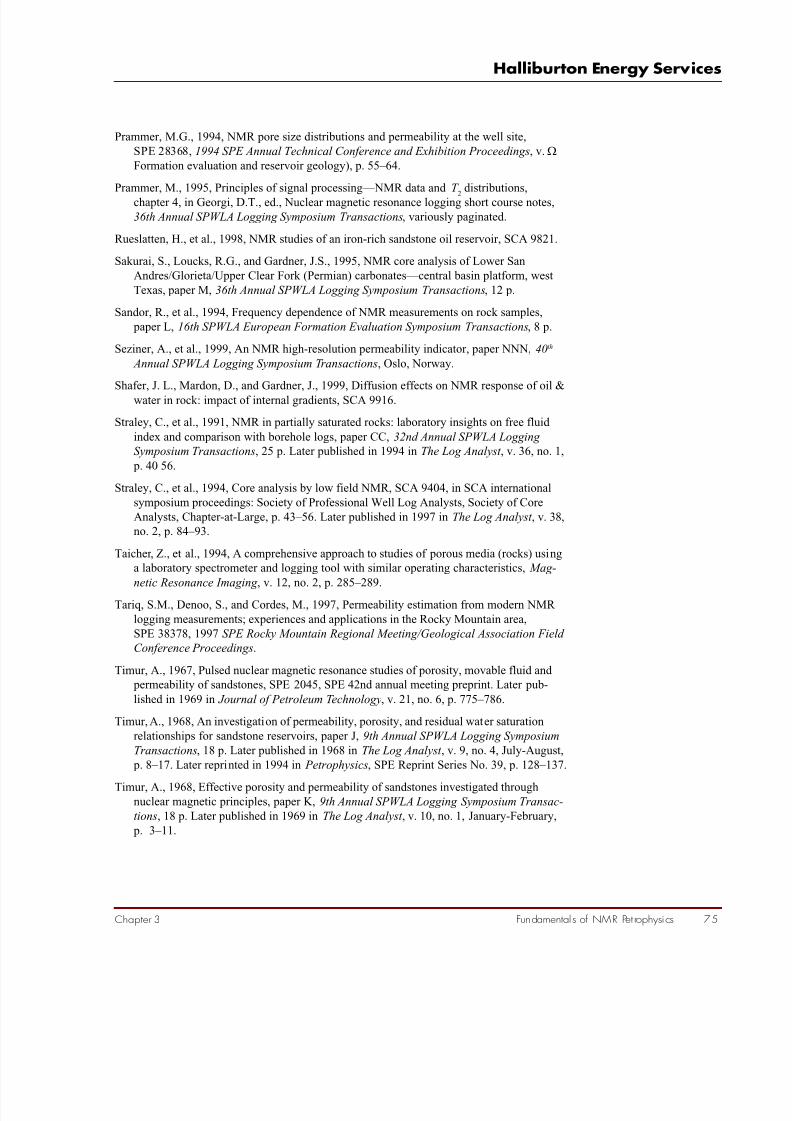
7/28/2019 NMR Logging Principles and Applications
http://slidepdf.com/reader/full/nmr-logging-principles-and-applications 93/253
Fundamentals of NMR Pet rophysics 75
Halliburton Energy Services
Chapter 3
Prammer, M.G., 1994, NMR pore size distributions and permeability at the well site,
SPE 28368, 1994 SPE Annual Technical Conference and Exhibition Proceedings, v. Ω
Formation evaluation and reservoir geology), p. 55–64.
Prammer, M., 1995, Principles of signal processing—NMR data and T 2
distributions,
chapter 4, in Georgi, D.T., ed., Nuclear magnetic resonance logging short course notes,
36th Annual SPWLA Logging Symposium Transactions, variously paginated.
Rueslatten, H., et al., 1998, NMR studies of an iron-rich sandstone oil reservoir, SCA 9821.
Sakurai, S., Loucks, R.G., and Gardner, J.S., 1995, NMR core analysis of Lower San
Andres/Glorieta/Upper Clear Fork (Permian) carbonates—central basin platform, west
Texas, paper M, 36th Annual SPWLA Logging Symposium Transactions, 12 p.
Sandor, R., et al., 1994, Frequency dependence of NMR measurements on rock samples,
paper L, 16th SPWLA European Formation Evaluation Symposium Transactions, 8 p.
Seziner, A., et al., 1999, An NMR high-resolution permeability indicator, paper NNN, 40th
Annual SPWLA Logging Symposium Transactions, Oslo, Norway.
Shafer, J. L., Mardon, D., and Gardner, J., 1999, Diffusion effects on NMR response of oil &
water in rock: impact of internal gradients, SCA 9916.
Straley, C., et al., 1991, NMR in partially saturated rocks: laboratory insights on free fluid
index and comparison with borehole logs, paper CC, 32nd Annual SPWLA Logging
Symposium Transactions, 25 p. Later published in 1994 in The Log Analyst , v. 36, no. 1,
p. 40 56.
Straley, C., et al., 1994, Core analysis by low field NMR, SCA 9404, in SCA international
symposium proceedings: Society of Professional Well Log Analysts, Society of Core
Analysts, Chapter-at-Large, p. 43–56. Later published in 1997 in The Log Analyst , v. 38,
no. 2, p. 84–93.
Taicher, Z., et al., 1994, A comprehensive approach to studies of porous media (rocks) using
a laboratory spectrometer and logging tool with similar operating characteristics, Mag-
netic Resonance Imaging , v. 12, no. 2, p. 285–289.
Tariq, S.M., Denoo, S., and Cordes, M., 1997, Permeability estimation from modern NMR
logging measurements; experiences and applications in the Rocky Mountain area,
SPE 38378, 1997 SPE Rocky Mountain Regional Meeting/Geological Association Field
Conference Proceedings.
Timur, A., 1967, Pulsed nuclear magnetic resonance studies of porosity, movable fluid and
permeability of sandstones, SPE 2045, SPE 42nd annual meeting preprint. Later pub-
lished in 1969 in Journal of Petroleum Technology, v. 21, no. 6, p. 775–786.
Timur, A., 1968, An investigation of permeability, porosity, and residual water saturation
relationships for sandstone reservoirs, paper J, 9th Annual SPWLA Logging Symposium
Transactions, 18 p. Later published in 1968 in The Log Analyst , v. 9, no. 4, July-August,
p. 8–17. Later reprinted in 1994 in Petrophysics, SPE Reprint Series No. 39, p. 128–137.
Timur, A., 1968, Effective porosity and permeability of sandstones investigated throughnuclear magnetic principles, paper K, 9th Annual SPWLA Logging Symposium Transac-
tions, 18 p. Later published in 1969 in The Log Analyst , v. 10, no. 1, January-February,
p. 3–11.

7/28/2019 NMR Logging Principles and Applications
http://slidepdf.com/reader/full/nmr-logging-principles-and-applications 94/253
NMR Logging Principles and Applications
76 Fundamentals of NMR Petrophysics Chapter 3
Timur, A., 1972, Nuclear magnetic resonance study of carbonates, paper N, 13th Annual
SPWLA Logging Symposium Transactions, 15 p. Later published in 1972 in The Log
Analyst , v. 13, no. 5, p. 3–11.
Tutunjian, P.N., et al., 1993, Characterization of pore microgeometry by NMR diffusion
measurements, paper II, in 34th Annual SPWLA Logging Symposium Transactions, 13 p.
Vinegar, H. J., et al., 1991, Whole-Core Analysis by 13C NMR, SPE Formation Evaluation,
p. 183–189.
Volokitin, Y., et al., 1999, Constructing capillary pressure curves from NMR log data in the
presence of hydrocarbons, 40th Annual SPWLA Logging Symposium Transactions.
Xiao, L.Z., 1998, NMR imaging logging principles and applications, Science Press (in
Chinese), Beijing, 328 p.
Zhang, Q., et al., 1998, Some exceptions to default NMR rock and fluid properties, FF, 39th
Annual SPWLA Logging Symposium Transactions.
Zhang, Q., Hirasaki, G. J., and House, W. V., 1998, Diffusion in internal field gradients,
SCA 9823.

7/28/2019 NMR Logging Principles and Applications
http://slidepdf.com/reader/full/nmr-logging-principles-and-applications 95/253
Fundamentals of NMR Hydrocarbon Typing 7
Halliburton Energy Service
Chapter 4
Fundamentalsof NMR HydrocarbonTyping
Chapter 4
The NMR properties of different reservoir fluids are quite different
from one another. These differences make it possible to type hydrocar-
bons and sometimes to quantify their volumes. This chapter first
reviews NMR properties of hydrocarbons and NMR hydrocarbon-
typing techniques based on T 1
relaxation and/or diffusivity contrast.
The chapter then discusses qualitative forward modeling of oil and gas
effects on T 2
distributions under different conditions.
NMR Properties of Hydrocarbons
NMR properties, such as the T 1
and T 2, of oil and gas at reservoir
conditions in a water-wet rock, can be calculated based on the equa-
tions introduced in Chapter 3. The T 1
and T 2
of dead oil and gas are
given in Eqs. 4.1 through 4.4.
Dead Oil
η
k T T 00713.0
1= (4.1)
( )12
2
5
1
1
2298
102.500713.0TE G T T
T K k γ ηη
−−
− ×+
= (4.2)
Gas
(4.3)
( )12
105.8105.2
29.07
1
17.1
41
2
TE G T
T T
g
k
k
g γ ρ
ρ
×+
×= −
−
−
................. (4.4)
12
ρ g
1.17T
1= 2.5 104
Τ k

7/28/2019 NMR Logging Principles and Applications
http://slidepdf.com/reader/full/nmr-logging-principles-and-applications 96/253
NMR Logging Principles and Applications
78 Fundamentals of NMR Hydrocarbon Typing Chapter 4
Eqs. 4.1 through 4.4 assume that the relaxation is given by the bulk fluid relaxation for T 1,
and that the T 2
relaxation is composed of a bulk relaxation term and a diffusion term. The
expressions for the diffusion coefficients—Eqs. 3.12 and 3.13—have been used in Eqs. 4.2
and 4.4. In the absence of diffusion, T 1and T
2are taken to be equal. The water-wet condition
implies that a layer of water coats the rock grains and thus prevents contact between the rock
grain and any hydrocarbon fluid. Consequently, there is no surface relaxation term. The lack of surface relaxation for oil in water-wet rocks is confirmed by numerous laboratory and
field observations. However, in a series of experiments, Straley in 19971 unexpectedly found
an apparent surface relaxation component for the relaxation of methane in both a sandstone
sample and a carbonate sample. At this time, the results have not been confirmed by work at
other laboratories, and no theoretical explanation for this observation has been published.
The surface relaxation component reported by Straley would have a minimal effect on gas
detection using the TDA method discussed in Chapter 6. That this effect would be minimal
can be verified by examination of the TDA equations found in the Chapter 6 Appendix.
In reality, the T 2
of crude oil is a distribution of values rather than a single value and depends
on viscosity.2,3 As viscosity increases, the hydrogen protons become less mobile and thus
relax more quickly. Therefore, increases in viscosity shorten the T 2
geometric mean. More
viscous oils usually also have broader T 2
distributions. The broadening is due to the different
mobilities of the protons in the different oil components. More viscous oils are often com-
posed of a wider variety of hydrocarbons. Even some light oils have multiple components
and can exhibit a broadened T 2
distribution. NMR T 2
measurements on several crude oils with
different viscosities are illustrated in Fig. 4.1.
The NMR response of gas is quite different from the responses of water and oil under typical
reservoir conditions.4, 5 NMR measurements can thus be used to quantify the gas phase in a
reservoir. Dry natural gas is composed mostly of methane (CH4), along with other light
hydrocarbons and often with small amounts of non-hydrocarbon substances. Fig. 4.2 shows
how the hydrogen index, diffusion coefficient, and T 1
and T 2
relaxation times of methane vary
with pressure and temperature.1, 6, 7
Table 4.1 is an example of NMR properties of bulk fluids, such as brine, oil, and gas, at
reservoir conditions.6
The differences in T 1, T 2, and D among these fluids at reservoir condition form the foundation for NMR fluid typing. Two methods of hydrocarbon typing
have been developed: dual-TW and dual-TE . The dual-TW method is based on the T 1
contrast
between water and light hydrocarbons. The dual-TE method is based on the diffusivity
difference between water and medium viscosity oil or between liquid and gas.
Table 4.1 —NMR Properties of Reservoir Fluids
Fluid
Brine
Oil
Gas
T 1
1 - 500
3,000 - 4,000
4,000 - 5,000
T 2
1 - 500
300 - 1,000
30 - 60
TypicalT 1 / T 2
2
4
80
Hl
1
1
0.2 - 0.4
h
(cp)
0.2 - 0.8
0.2 - 1,000
0.011 - 0.014methane
D 0 x 10-5
(cm2 /s)
1.8 - 7
0.0015 - 7.6
80 - 100
(ms) (ms)
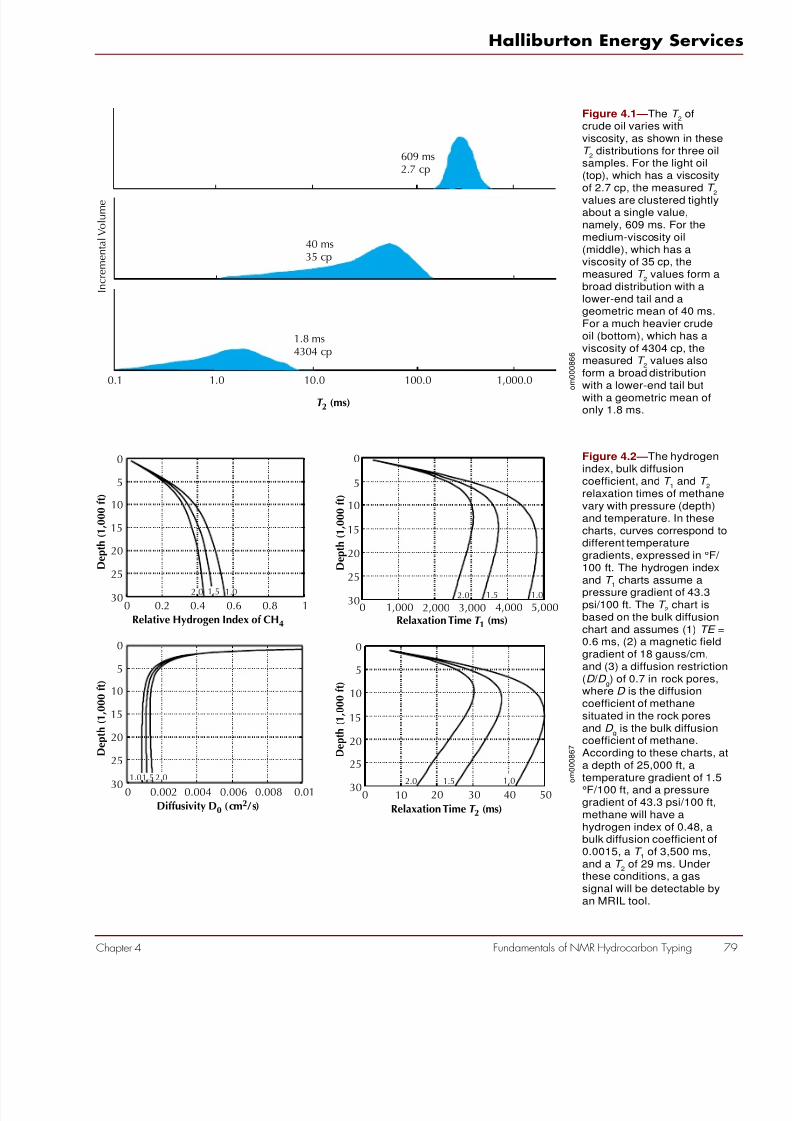
7/28/2019 NMR Logging Principles and Applications
http://slidepdf.com/reader/full/nmr-logging-principles-and-applications 97/253
Fundamentals of NMR Hydrocarbon Typing 7
Halliburton Energy Service
Chapter 4
Figure 4.2—The hydrogenindex, bulk diffusioncoefficient, and T
1and T
2
relaxation times of methanevary with pressure (depth)and temperature. In thesecharts, curves correspond todifferent temperaturegradients, expressed in °F/ 100 ft. The hydrogen indexand T
1charts assume a
pressure gradient of 43.3psi/100 ft. The T
2chart is
based on the bulk diffusionchart and assumes (1) TE =0.6 ms, (2) a magnetic fieldgradient of 18 gauss/cm,and (3) a diffusion restriction(D / D
g) of 0.7 in rock pores,
where D is the diffusioncoefficient of methanesituated in the rock poresand D
gis the bulk diffusion
coefficient of methane.According to these charts, ata depth of 25,000 ft, atemperature gradient of 1.5
°F/100 ft, and a pressuregradient of 43.3 psi/100 ft,methane will have ahydrogen index of 0.48, abulk diffusion coefficient of0.0015, a T
1of 3,500 ms,
and a T 2
of 29 ms. Underthese conditions, a gassignal will be detectable byan MRIL tool.
5 5
10 10
15 15
20 20
25 25
30 300 00.2 0.4 2,0000.6 3,0000.8 4,0001 5,000
0 0
1.0 1.0
2.0
2.0 1.5
1.52.0
1.0
1.0
2.0
1,000
Depth(1,000ft)
Depth(1,000ft)
Relative Hydrogen Index of CH4 Relaxation Time T 1 (ms)
5 5
10 10
15 15
20 20
25 25
30 300 00.002 100.004 200.006 300.008 400.01 50
0 0
Depth(1,000ft)
Depth(1,000ft)
Diffusivity D02(cm /s) Relaxation Time T 2 (ms)
1.5
1.5
o m
0 0 0 8 6 7
Figure 4.1 —The T 2
ofcrude oil varies withviscosity, as shown in theseT
2distributions for three oil
samples. For the light oil(top), which has a viscosityof 2.7 cp, the measured T
2
values are clustered tightlyabout a single value,namely, 609 ms. For themedium-viscosity oil(middle), which has aviscosity of 35 cp, themeasured T
2values form a
broad distribution with alower-end tail and ageometric mean of 40 ms.For a much heavier crudeoil (bottom), which has aviscosity of 4304 cp, themeasured T
2values also
form a broad distribution
with a lower-end tail butwith a geometric mean ofonly 1.8 ms.
609 ms2.7 cp
40 ms35 cp
1.8 ms4304 cp
0.1 1.0 10.0 100.0 1,000.0
T 2 (ms)
I n c r e m e n t a l V o l u m e
o m
0 0 0 8 6 6

7/28/2019 NMR Logging Principles and Applications
http://slidepdf.com/reader/full/nmr-logging-principles-and-applications 98/253
NMR Logging Principles and Applications
80 Fundamentals of NMR Hydrocarbon Typing Chapter 4
NMR Hydrocarbon Typing
T 2Distribution of a Partially Saturated Rock
As was illustrated in Fig. 3.11, a single pore, fully saturated with water, exhibits a sharp peak
at a moderate T 2
value on the T 2
distribution. As the movable water is displaced by oil, the
single peak on the T 2
distribution separates into two peaks. One peak often appears as a very
low amplitude peak below the original T 2
value and is attributable to irreducible water in
smaller pores and on the pore surface. The other peak, which appears above the original T 2
value, is attributable to the oil, and the T 2
value of this peak is close to the T 2
of bulk oil. This
phenomenon is shown in Fig. 4.3 for a North Sea chalk. North Sea chalks exhibit an unusu-
ally large amount of irreducible water associated with the pore surface.
T 1Relaxation Contrast
Table 4.1 and Eqs. 4.1 and 4.3 show that gas and oil each have T 1
relaxation times much
longer than that of brine. Therefore, for full polarization, a longer TW is needed for hydrocar-
bons than for water. Dual-TW measurements are based on the T 1
contrast between water and
light hydrocarbons, and are made using two TW values, TW short
and TW long
.
For the short TW ,
( ) ( )
s gaT t
gasT short TW
gasoil T
t
oil T short TW
oil
wiT t
wiT short TW
i short TW
ee M ee M
ee M t M
2121
2
11
101
−
−+
−+
−=
−−−
−−
∑
(4.5)
For the long TW ,
( ) ( )
gasT t
gasT long TW
gasoil T
t
oil T long TW
oil
wiT t
wiT long TW
ilong TW
ee M ee M
ee M t M
2121
21
11
10
−−
−−
−−
−+
−+
−= ∑
(4.6)
where, T 1wi
and T 2wi
are the T 1
and T 2
of water in the ith bin respectively.
Fig. 4.4 illustrates the dual-TW method. A TW of three times T 1
is required to achieve 95%
polarization. The maximum T 1
of water in sandstone pores is about 0.5 s, and the minimum T 1
of light hydrocarbons is about 3 s. Therefore, water will be fully polarized by using a TW short
at least 1.5 s (Fig. 4.4, upper left), and hydrocarbons will be adequately polarized in many
cases by using a TW long
of 9 s (Fig. 4.4, upper right). (TW long
may need to be adjusted for the
hydrocarbon pressure and temperature, and for gas it may not be practical to achieve com-
plete polarization.) Because water is fully polarized at both the short and long polarization

7/28/2019 NMR Logging Principles and Applications
http://slidepdf.com/reader/full/nmr-logging-principles-and-applications 99/253
Fundamentals of NMR Hydrocarbon Typing 8
Halliburton Energy Service
Chapter 4
Figure 4.3 —A North Seachalk sample demon-strates how T
2distributions
vary with water saturation.At S
w = 100%, the sample
exhibits a simple pore-sizedistribution: the signal is
mainly focused at T 2 = 27ms, indicating essentiallyone pore size. As S
w
decreases (oil saturationincreases), the amplitudeof the water peak of the T
2
distribution decreasesbecause of the decreasingvolume of water. Theamplitude of the oil peak atabout 200 ms increasesbecause of the increasingoil volume. Furthermore,because the surface-to-volume ratio of the watersignal is changing (assum-
ing that pore surface arearemains the same and thatsurface relaxivity does notchange, but that watervolume is decreasing), theT
2value for the water
also decreases.
o m
0 0 0 8 6 5
Figure 4.4 —In the dual-TW measurement, onlywater can fully polarize
during TW short, while bothwater and hydrocarbonscan fully polarize duringTW
long. Results obtained by
taking the differencebetween the resulting T
2
distributions are used todetect and quantifyhydrocarbons.
TW long
TW short
TW short TW long
T 1 Relaxation Contrast Mechanism
T 2 Distibution
Hydrocarbon
Water
0
Polarization and Echo Acquisition Time (s)
1 110 10100 1001,000 1,000T 2 (ms) T 2 (ms)
Amplitude
o m
0 0 0 8 6 9
4.0
3.0
2.0
1.0
0.00.6
2.17.4
26.695.4
341.8
1,224.8T 2 Distribution
I ncrementalPorosity%
Sw = 100%
Sw = 84.3%
Sw = 56.9%
Sw = 65.4%

7/28/2019 NMR Logging Principles and Applications
http://slidepdf.com/reader/full/nmr-logging-principles-and-applications 100/253
NMR Logging Principles and Applications
82 Fundamentals of NMR Hydrocarbon Typing Chapter 4
times, it will have the same amplitude on the resulting T 2
distributions (Fig. 4.4, bottom).
However, light hydrocarbons will be fully polarized only when TW long
is used. Therefore, the
difference of the two T 2
distributions acquired with TW long
and TW short
will leave only the
hydrocarbon components. Thus, light hydrocarbons can be detected and quantified, the
methods of which will be discussed in Chapter 6.
Diffusivity Contrast
T 2diffusion
depends on D, G , and TE . For brines, medium-viscosity oils, and heavy oils, Dgas
is
much greater than Dw, and the D
wis much greater than D
oil. (See Table 4.1.) Thus, T
2diffusionwill
be very different among these fluids, and the differences can be amplified by NMR measure-
ments made with different TE . Dual-TE measurements use two TE values, TE short
and TE long
.
For the short TE ,
( ) ( )( )
( ) ( )
−−
+−−
++−−
−+
−+
−= ∑
12112
1
1
122
1
1
22
2
11
10
2
short TE G gas Dt
gasT TW
gas
short TE G D
T t
oil T TW
oil
short TE G w D
V
S
wT t
wiT TW
i short TE
ee M ee M
ee M t M
oil
oil
γ γ
γ ρ
(4.7)
When TW >> 3xmax (T 1w , T
1oil , T
1gas) ,
( ) ( )( )
( ) ( )
−
+−
++−
++
=
∑1212
2
1
122
1
22
2
0
short TE G gas Dt
gas
short TE G
oil D
oil T t
oil
short TE G w D
V
S
wT t
i short
TE
e M e M
e M t M
γ γ
γ ρ
(4.8)
For the long TE ,
( ) ( )
−
+−
−
++−−
−+
−+
−= ∑
12
1
122
1
1
122
1
1
22
2
11
10
long TE G
gas Dt
gasT TW -
gas
long TE G
oil D
oil T t
oil T TW
oil
long TE G
w DV
S
wT t
wiT TW
ilong TE
ee M ee M
ee M t M
γ γ
γ ρ
(4.9)

7/28/2019 NMR Logging Principles and Applications
http://slidepdf.com/reader/full/nmr-logging-principles-and-applications 101/253
Fundamentals of NMR Hydrocarbon Typing 8
Halliburton Energy Service
Chapter 4
When TW >> 3xmax(T 1w
, T 1oil
, T 1 gas
),
( ) ( )
−
+−
++−
++
= ∑1212
2
1
122
1
22
2
0
long TE G
gas Dt
gas
long TE G
D
oil T
t
oil
long TE G
w DV
S
wT t
ilong
TE
e M e M
e M t M
oil
γ γ
γ ρ
(4.10)
Fig. 4.5 illustrates a dual-TE measurement in which TE long
= 3 TE short
. The pore fluid is
assumed to be composed of two phases, one with large D (the green component of the echo
trains in the figure) and one with small D (the red component of the echo trains). The
difference in the decay of a particular component between the TE short
and TE long
measurements
is greater for the component with the larger D. Specifically, the large- D component decays
much more quickly during the TE long
measurements than during the TE short
measurements,
while the small- D component decays only slightly faster during the TE long
measurements than
during the TE short
measurements. This distinction between the two components is reflected in
the corresponding T 2
distributions and can be used to distinguish the fluids.
Numerical Simulations
NMR responses for dual-TW or dual-TE measurements can be numerically simulated with
the equations presented earlier in this section.8 This simulation is important for job planning
(Chapter 8) and for interpreting dual-TW and dual-TE logs (Chapter 6).
Figure 4.5 —In this dual-TE measurement of a two-phase pore fluid, the echo-train of the large-D fluid(green curve) decaysmuch faster during TE
long
measurements than duringTE
shortmeasurements. The
decay of the fluid with thesmall-D component (redcurve) increases onlyslightly during TE
long
measurements. These
decay differences arereflected in the T 2
distribu-tions and can be used todistinguish the fluids.
Diffusivity Contrast Mechanism
T 2 Distibution
1 110 10100 1001,000 1,000T 2 (ms) T 2 (ms)
TE short
TE short TE long
TE long
Polarization and EchoAcquisition
Time (s)
TW TW
A m p
l i t u d
e
o m
0 0 0 8 7 0
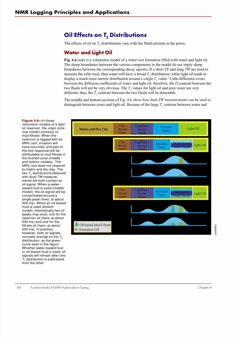
7/28/2019 NMR Logging Principles and Applications
http://slidepdf.com/reader/full/nmr-logging-principles-and-applications 102/253
NMR Logging Principles and Applications
84 Fundamentals of NMR Hydrocarbon Typing Chapter 4
Figure 4.6 —In thesevolumetric models of a light-oil reservoir, the virgin zone(top model) contains nomud filtrate. When thereservoir is logged with anMRIL tool, invasion willhave occurred, and part ofthe tool response will beattributable to mud filtrate inthe flushed zone (middleand bottom models). TheMRIL tool does not respondto matrix and dry clay. Thetwo T
2distributions obtained
with dual-TW measure-ments will both contain anoil signal. When a water-based mud is used (middlemodel), the oil signal will beconcentrated around asingle peak (here, at about500 ms). When an oil-basedmud is used (bottommodel), theoretically two oilpeaks may exist, one for thereservoir oil (here, at about500 ms) and one for thefiltrate oil (here, at about200 ms). In practice,however, both oil signals
normally overlap on theT
2distribution, as the greencurve seen in the figure.Whether water-based mudor oil-based mud is used, oilsignals will remain after oneT
2distribution is subtracted
from the other.
Matrix and Dry Clay
Clay-boundWater
Capillary-boundWater
MovableWater
MovableWater
Water-based Mud
Light Oil
Light Oil
Clay-boundWater
Capillary-boundWater
Oil-based Mud Clay-boundWater
Capillary-boundWater
Light Oil
Porosity
Porosity
Short TW
Long TW
1 10 100 1,000 T 2 (ms)
Porosity
Porosity
Short TW
Long TW
1 10 100 1,000T 2 (ms)Formation Oil
Oil-based Mud Filtrate
Oil-basedMud Filtrate
Water-basedMud Filtrate
MovableWater
o m
0 0 0 8 7 1
Oil Effects on T 2 Distributions
The effects of oil on T 2
distributions vary with the fluids present in the pores.
Water and Light Oil
Fig. 4.6 (top) is a volumetric model of a water-wet formation filled with water and light oil.The sharp boundaries between the various components in the model do not imply sharp
boundaries between the corresponding decay spectra. If a short TE and long TW are used to
measure the echo train, then water will have a broad T 2
distribution, while light oil tends to
display a much more narrow distribution around a single T 2
value.3 Little difference exists
between the diffusion coefficients of water and light oil; therefore, the D contrast between the
two fluids will not be very obvious. The T 1
values for light oil and pore water are very
different; thus, the T 1
contrast between the two fluids will be detectable.
The middle and bottom sections of Fig. 4.6 show how dual-TW measurements can be used to
distinguish between water and light oil. Because of the large T 1
contrast between water and

7/28/2019 NMR Logging Principles and Applications
http://slidepdf.com/reader/full/nmr-logging-principles-and-applications 103/253
Fundamentals of NMR Hydrocarbon Typing 8
Halliburton Energy Service
Chapter 4
light oil, the water signal will disappear when the TW short
and TW long
T 2
distributions are
subtracted from one another. The resulting differential “spectrum” will contain only part of
the light-oil signal. The amplitude of this signal in the differential spectrum will be highly
dependent on both the T 1
difference between the two kinds of fluids and the difference
between TW short
and TW long
. Normally, TW short
and TW long
are selected so that TW short
≥
3T 1,bulk water and TW long ≥
3T 1,light oil. If oil-based mud is used, a signal from the mud filtrate willappear on the T 2
distribution. In Fig. 4.6, the T 2
of light oil is concentrated at about 500 ms.
The T 2 of oil-based mud filtrate is about 200 ms. The signals from both light oil and oil-based
mud filtrate will remain in the differential spectrum. Normally, it is difficult to distinguish
the native oil and oil-based mud filtrate because of the mixture of these two kinds of oil and
their NMR signals.
Water and Viscous Oil
When both water and viscous oil fill the pores of a water-wet formation, the volumetric
model of the formation can be illustrated as in Fig. 4.7. If a small TE and long TW are used,
the spin-echo signal from water measured with the MRIL gradient field will usually have a
broad T 2
distribution, and the signal from viscous oil will also typically have a broad T 2
distribution. The bulk decay time T 2
for viscous oil and the contribution to the decay time of
water from surface relaxation usually are not very different. The diffusion coefficients for
both water and viscous oil, however, are very different; therefore, the diffusion contrast
between the two fluids is detectable.
Fig. 4.7 shows how dual-TE measurements can be used to distinguish between water and
viscous oil. Because of the diffusion contrast between water and viscous oil, the T 2
distribu-
tion measured with TE long
will show a much larger shift to the left (to lower T 2
values) for
water than for viscous oil, as compared to the T 2
distribution measured with TE short
. The fast
T 2times of water will shift very little. When oil-based mud is used, normally it has lower
viscosity than viscous oil at reservoir conditions. The T 2
components of an oil-based mud
filtrate measured with TE short
will be clustered around a single peak with T 2
longer than that of
viscous oil. The T 2 peak of an oil-based mud filtrate measured with TE
long, however, may be
shorter than that of viscous oil because of the high diffusivity of the filtrate. Careful selection
of TE long makes it possible to separate the T 2 components of viscous oil and water, whether water-based or oil-based mud is used in the well. In general, because the diffusion shift is
non-linear, relaxation times longer than the diffusion relaxation time will shift much more to
the left than those shorter than the diffusion relaxation time. This non-linear shifting thus
causes the spectra to become more sharply peaked as diffusion increases.
Effects of Viscosity and Wettability on the Oil Signalin a T
2Distribution
In the discussion thus far, the formations have been assumed to be water-wet. If the forma-
tion logged by an NMR tool is not water-wet but instead is partially or completely oil-wet,
then the oil T 2
values will be different and the T 2
distributions will be different from those
discussed earlier.8, 9 Rocks are probably never completely oil-wet; some are of intermediate
and/or mixed wettability. Mixed wettability most likely occurs in reservoir rocks where oil
has been trapped and comes into contact with the grain surfaces in the larger pores to form
an oil film or coating on the grains. Crude oils vary in their ability to alter the wettability of a
pore surface. The pore surfaces of the smaller pores or in the crevices of larger pores are not
in contact with the oil and remain water-wet. For NMR, the essential condition for water
wettability is the existence of a protective layer of water between the rock grain and the
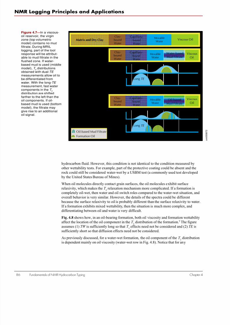
7/28/2019 NMR Logging Principles and Applications
http://slidepdf.com/reader/full/nmr-logging-principles-and-applications 104/253
NMR Logging Principles and Applications
86 Fundamentals of NMR Hydrocarbon Typing Chapter 4
hydrocarbon fluid. However, this condition is not identical to the condition measured by
other wettability tests. For example, part of the protective coating could be absent and the
rock could still be considered water-wet by a USBM test (a commonly used test developed
by the United States Bureau of Mines).
When oil molecules directly contact grain surfaces, the oil molecules exhibit surface
relaxivity, which makes the T 2
relaxation mechanism more complicated. If a formation is
completely oil-wet, then water and oil switch roles compared to the water-wet situation, and
overall behavior is very similar. However, the details of the spectra could be different
because the surface relaxivity to oil is probably different than the surface relaxivity to water.
If a formation exhibits mixed wettability, then the situation is much more complex, and
differentiating between oil and water is very difficult.
Fig. 4.8 shows how, in an oil-bearing formation, both oil viscosity and formation wettability
affect the location of the oil component in the T 2
distribution of the formation.7 The figure
assumes (1) TW is sufficiently long so that T 1 effects need not be considered and (2) TE issufficiently short so that diffusion effects need not be considered.
As previously discussed, for a water-wet formation, the oil component of the T 2
distribution
is dependent mainly on oil viscosity (water-wet row in Fig. 4.8). Notice that for any
Figure 4.7 —In a viscous-oil reservoir, the virginzone (top volumetricmodel) contains no mudfiltrate. During MRILlogging, part of the toolresponse will be attribut-
able to mud filtrate in theflushed zone. If water-based mud is used (middlemodel), T
2distributions
obtained with dual-TE
measurements allow oil tobe differentiated fromwater. With the long-TE
measurement, fast watercomponents in the T
2
distribution are shiftedfarther to the left than theoil components. If oil-based mud is used (bottommodel), the filtrate maygive rise to an additional
oil signal.
Matrix and Dry Clay
Clay-
boundWater
Capillary-boundWater
MovableWater
Movable
Water
Oil-basedMud Filtrate
Water-based Mud
Viscous Oil
Viscous
Oil
Clay-boundWater
Capillary-boundWater
Oil-based Mud Clay-boundWater
Capillary-
boundWater
Water-based
Mud Filtrate
Porosity
Porosity
1 10 100 1,000T 2 (ms)
Porosity
Porosity
Short TW
Short TE
1 10 100 1,000T 2 (ms)Formation Oil
Oil-based Mud Filtrate
ViscousOil
Long TE
Short TE
MovableWater
Long TE
o m
0 0 0 8 7 2

7/28/2019 NMR Logging Principles and Applications
http://slidepdf.com/reader/full/nmr-logging-principles-and-applications 105/253
Fundamentals of NMR Hydrocarbon Typing 8
Halliburton Energy Service
Chapter 4
wettability, the heavy-oil component of the T 2
distribution is broad and fills the BVI portion
of the distribution (heavy-oil column in Fig. 4.8), which makes detecting heavy oil with
MRIL measurements difficult. For a mixed-wet formation, which poses one of the greatest
challenges for MRIL applications, the oil and water components of the T 2
distribution are
broad and overlap each other (mixed-wet row in Fig. 4.8). Although this overlapping does not
affect the total porosity estimation, it will affect the determination of BVI, free fluid, perme-ability, and, of course, the hydrocarbon type. For the rare oil-wet formation, oil molecules
will be adsorbed on all pore surfaces. In this case, BVI will be the bulk volume irreducible of
oil. The water component will be always in the free-fluid portion of the distribution (oil-wet
row of Fig. 4.8) and should exhibit bulk characteristics. The T 1and T
2of water are both
single-valued and quite long compared to the corresponding relaxation times of the oil in
contact with the pore wall.
Gas Effects on T 2Distribution Under
Different Conditions
Gas is always a non-wetting phase in the pore space of a formation. Hence, the T 1
of gas is
taken as that of bulk gas (Straley’s work 1 suggests that sometimes this assumption may be too
simple), which is much longer than the T 1
of water in contact with the pore wall. The T 2diffusion
of gas will dominate the T 2
of gas. These characteristics and the gradient field of the MRIL
tool make the gas signal detectable through MRIL measurements.
Figure 4.8 —The positionand breadth of the oilcomponent in the T
2
distribution of a formationdepends on oil viscosityand formation wettability.Oil typing is easiest in
water-wet formationsbecause of the moderatebreadth and distinctpositions of the different oilcomponents in the T
2
distribution. Oil typing ismost difficult in mixed-wetformations because the oiland water componentsare broad and overlapeach other.
Heavy OilMedium-Viscosity OilLight Oil
Oil
Formation
Water-wet
Mixed-wet
Oil-wet
Oil Signal Water Signal
o
m 0 0 0 8 7 3

7/28/2019 NMR Logging Principles and Applications
http://slidepdf.com/reader/full/nmr-logging-principles-and-applications 106/253
NMR Logging Principles and Applications
88 Fundamentals of NMR Hydrocarbon Typing Chapter 4
Water and Gas
Fig. 4.9 presents volumetric models for rocks saturated by water and gas. The models depict
a virgin zone and zones invaded by water-based and oil-based muds. If a small TE and long
TW are used, the spin-echo signal from water will have a broad T 2
distribution, while the
signal from gas will have almost a single T 2
value. The T 1
times for water and gas are very
different; therefore, the T 1 contrast can be used to differentiate water and gas, as shown in themiddle and bottom models of Fig. 4.9.
As with water and light oil, a large T 1
contrast exists between gas and water in contact with
the pore wall. Thus, when dual-TW measurements (see Chapter 6) are used, and the resulting
T 2
distributions are subtracted from one another, the water component will be eliminated, and
part of the gas component will remain in the differential spectrum. The amplitude of the
partial gas component in the differential spectrum will be highly dependent on both the
difference between T 1gas
and T 1w
and the difference between TW short
and TW long
. Normally,
logging parameters are set so that TW long
≥ T 1gas
and TW short
≥ 3T 1w
. In addition, when gas is
present, hydrogen index and polarization effects must be considered because gas has low
hydrogen index and long T 1.
If oil-based mud is used, a signal from the oil-based mud filtrate appears on the T 2 distribu-tion. In Fig. 4.9, the T 2
of the gas is concentrated at about 40 ms, and the T 2 of oil-based mud
filtrate is at about 200 ms. The signals from both gas and oil-based mud filtrate will remain in
the differential spectrum.
Figure 4.9 —In a gasreservoir, the virgin zone(top volumetric model)contains no mud filtrate.During NMR logging, part of
the tool response will beattributable to mud filtrate inthe flushed zone. Whenwater-based mud and dual-TW measurements areused (middle model), gascan be detected bysubtracting the two resultingT
2distributions. If oil-based
mud is used (bottommodel), the resultingdifferential spectrum willalso contain a componentattributable to the oil-basedfiltrate that has invaded theformation.
Matrix and Dry Clay
Clay-boundWater
Capillary-boundWater
MovableWater
MovableWater
Water-based Mud
Gas
Gas
Clay-boundWater
Capillary-boundWater
Oil-based Mud Clay-boundWater
Capillary-boundWater
Gas
Porosity
Porosity
Short TW
Long TW
1 10 100 1,000T 2 (ms)
Porosity
Porosity
Short TW
Long TW
1 10 100 1,000T 2 (ms)Formation Gas
Oil-based Mud Filtrate
Water-basedMud Filtrate
MovableWater
Oil-basedMud Filtrate
o m
0 0 0 8 7 4

7/28/2019 NMR Logging Principles and Applications
http://slidepdf.com/reader/full/nmr-logging-principles-and-applications 107/253
Fundamentals of NMR Hydrocarbon Typing 8
Halliburton Energy Service
Chapter 4
Water, Light Oil, and Gas
When water, light oil, and gas occupy the same pore system in the formation rocks ( Fig.
4.10), both light oil and gas can still be detected through their T 1
contrast. Dual-TW measure-
ments are used, and TW long
should be greater than three times of the maximum T 1
of light oil,
gas, and (if oil-based mud is used) the oil-based mud filtrate. When oil-based mud is
used, the signals from light oil, gas, and oil-based mud filtrate will remain in thedifferential spectrum.
Although the difference in diffusivity between gas and liquid is large, this contrast is seldom
applied to separate the signals of two fluids. Generally, the T 2
of gas is very small. In most
cases, the gas T 2
component may fill the BVI window. When a longer TE is used, the gas
component may disappear from the T 2
distribution. The T 2
of gas is strongly affected by inter-
echo spacing in a gradient field. By carefully choosing TE and gradient strength (which is
related to frequency), the gas signal can be separated from BVI , light oil, and oil-based mud
filtrate. This choice is one of the keys for designing a T 1-contrast (i.e., dual-TW ) NMR
logging job.
Figure 4.10 —In a reser-voir containing gas andlight oil, the virgin zone(top volumetric model)contains no mud filtrate.During NMR logging, partof the tool response will beattributable to mud filtratein the flushed zone. Whenwater-based mud anddual-TW measurementsare used (middle model),gas and light oil can bedifferentiated from waterby subtracting the two
resultingT
2 distributions. Ifoil-based mud is used(bottom model), theresulting differentialspectrum may also containa component attributableto the oil-based filtrate thathas invaded the formation.The differentiation betweengas and light oil/oil-basedmud filtrate is dependenton resolvable T
2differ-
ences in the differentialspectrum.
LightOil
Gas
Matrix and Dry Clay
Clay-boundWater
Capillary-boundWater
MovableWater
MovableWater
Water-based Mud
Light Oil
LightOil
Clay-boundWater
Capillary-boundWater
Oil-based Mud Clay-boundWater
Capillary-boundWater
Porosity
Porosity
Short TW
Long TW
1 10 100 1,000T 2 (ms)
Porosity
Porosity
Short TW
Long TW
1 10 100 1,000T 2 (ms)
Formation Oil andOil-based Mud Filtrate
Gas
Oil-basedMud Filtrate
Water-basedMud Filtrate
MovableWater
Gas
Gas
Formation Oil
o m
0 0 0 8 7 5
References
1. Straley, C., 1997, An experimental investigation of methane in rock materials, paper AA,
38th Annual SPWLA Logging Symposium Transactions, 14 p.
2. Kleinberg, R.L., and Vinegar, H.J., 1996, NMR properties of reservoir fluids, The Log
Analyst , v. 37, no. 6, p. 20–32.

7/28/2019 NMR Logging Principles and Applications
http://slidepdf.com/reader/full/nmr-logging-principles-and-applications 108/253
NMR Logging Principles and Applications
90 Fundamentals of NMR Hydrocarbon Typing Chapter 4
3. Morris, C. E., et al., 1997 Hydrocarbon saturation and viscosity estimation from NMR
logging in the Belridge diatomite, The Log Analyst , March-April, p. 44–59.
4. Gerritsma, C.J., Oosting, P.H., and Trappeniers, N.J., 1971, Proton spin-lattice relaxation
and self-diffusion in methane, part 2—Experimental results for proton spin-lattice
relaxation times, Physica, v. 51, p. 381–394.
5. Gerritsma, C.J., and Trappeniers, N.J., 1971, Proton spin-lattice relaxation and self-
diffusion in methanes, part 1—Spin-echo spectrometer and preparation of the methane
samples, Physica, v. 51, p. 365-380.
6. Akkurt, R., et al., 1995, NMR logging of natural gas reservoirs, paper N, 36th Annual
SPWLA Logging Symposium Transactions, 12 p. Later published in 1996, as Akkurt, R.,
et al. in The Log Analyst , v. 37, no. 5, p. 33–42.
7. Prammer, M.G., Mardon, D., Coates, G.R., and Miller, M.N., 1995, Lithology-indepen-
dent gas detection by gradient-NMR logging, SPE 30562, 1995 SPE Annual Technical
Conference and Exhibition Proceedings, v.Ω (Formation evaluation and reservoir
geology), p. 325–336.
8. Xiao, L.Z., 1998, NMR Imaging Logging Principles and Applications (in Chinese),Science Press, Beijing, 328 p.
9. Howard, J.J., and Spinler, E.A., 1993, Nuclear magnetic resonance measurements of
wettability and fluid saturations in chalk, SPE 26471, 1993 SPE Annual Technical
Conference and Exhibition Proceedings, v.Ω (Formation evaluation and reservoir
geology) p. 565–573. Later published in 1995 in SPE Advanced Technology Series, v. 3,
no. 1, p. 60–65.

7/28/2019 NMR Logging Principles and Applications
http://slidepdf.com/reader/full/nmr-logging-principles-and-applications 109/253
MRIL Tool Principles 91
Halliburton Energy Services
Chapter 5
MRIL ToolPrinciples
Chapter 5
The MRIL measurement process consists of four basic steps:
1. Polarizing the nuclei
2. Tipping the magnetization
3. Detecting spin echoes
4. Re-polarizing the nuclei
This chapter discusses the MRIL measurement process and associated
issues, such as vertical resolution, depth of investigation, signal-to-
noise ratio, and activation.
Polarization
An MRIL tool contains a large permanent magnet that produces a static
magnetic field.1,2 Before an earth formation is logged with an MRIL
tool, the hydrogen nuclei of the formation are aligned with the earth’s
magnetic field. Because the magnitude of the earth’s field is relatively
small, the magnitude of the magnetization induced in the protons is
also small. As an MRIL tool moves through the formation, the high-
magnitude field B0
of the tool dominates and polarizes the protons
(that is, it aligns them with the B0 field). For example, the strength of the earth’s field is about 0.5 gauss, while the strength of the MRIL-
produced magnetic field at the sensitive volume is about 176 gauss,
which is 350 times stronger than the earth’s magnetic field. For protons
in pore fluids, “full” polarization requires up to several seconds and
can be achieved as the tool moves through the wellbore. Reliable
measurements are made provided the protons are exposed to the same
static magnetic field throughout the entire measurement cycle. Fig. 5.1
shows the increase in polarization with time. Once the protons are
polarized, they are in an equilibrium state and will remain polarized
unless disturbed. The net magnetic moment of the polarized proton
population is M 0, which was discussed in Chapter 2.
Magnetization Tipping and Spin-EchoDetection
The MRIL technique of tipping the magnetization and acquiring spin
echoes from a formation is illustrated in Fig. 5.2. An MRIL tool
produces a static magnetic field with gradient in the radial direction;
therefore, the Larmor frequency of protons will vary with the radial

7/28/2019 NMR Logging Principles and Applications
http://slidepdf.com/reader/full/nmr-logging-principles-and-applications 110/253
NMR Logging Principles and Applications
92 MRIL Tool Principles Chapter 5
Figure 5.1— (1) Beforeprotons are subjected to theMRIL static magnetic field,
their spin axes are randomlyaligned. (2) Upon initialexposure of the protons tothe MRIL static magnetic
field, their spin axes begin toprecess, with the preces-sional axes being aligned
with the direction of thestatic field B
0(r) . (3 and 4) As
exposure continues, the spin
axes approach the preces-sional axes, and the netmagnetization of the protonpopulation increases, as the
graph indicates.
Figure 5.2— The MRIL
antenna (left) applies a 90°
oscillating B1
pulse tophase-synchronized
protons and tips themagnetization 90°. As theprotons dephase, the MRIL
antenna (middle) applies a180° oscillating B
1 pulse to
re-phase the protons.When the protons re-
phase (right), theygenerate a signal—a spinecho—which is measur-
able by the MRIL antenna.
o m
0 0 0 8 5 3
o m
0 0 0 8 7 6
1 2 3 4
0 2 4 6 8 10 12 14 16 18
Time (ms)
0
M 0
A m p
l i t u d e

7/28/2019 NMR Logging Principles and Applications
http://slidepdf.com/reader/full/nmr-logging-principles-and-applications 111/253
MRIL Tool Principles 93
Halliburton Energy Services
Chapter 5
distance from the tool.1,2 An antenna, which surrounds the magnet of the tool, serves as
oscillating-field transmitter and spin-echo receiver. The antenna produces a B1
field that is
perpendicular to B0
and that rotates the magnetization vector into the transverse plane. The
values selected for the frequency and bandwidth of the B1-field pulses determine the geom-
etry of the sensitive volume and, thus, the depth of investigation of the tool.
The MRIL tool records a spin-echo train, as illustrated in Fig. 5.3. The CPMG pulse se-
quence negates the dephasing caused by the gradient effects of the B0
field; however, the
dephasing that results from molecular interaction or diffusion processes is irreversible. When
this irreversible dephasing occurs, the protons can no longer be completely refocused, and
the CPMG spin-echo train decays. An MRIL tool measures the amplitude of the spin echoes
in the CPMG sequence to monitor the transverse magnetization decay and thus the irrevers-
ible dephasing. After a spin-echo train is acquired, the magnet repeats the polarization for the
next CPMG measurement, as illustrated in Fig. 5.4.
Figure 5.3 —To generate
and receive a spin-echotrain, an MRIL tool emits
a 90° B1 pulse followedby a sequence of 180°B
1pulses.
90° 180°
Time (ms)
180° 180° 180°TE
TE
Time (ms)
Antenna
Magnet Mandrel
S N
S N
Echo Signal
RF Pulse
o m
0 0 0 8 7 7
Figure 5.4 —The MRILmeasurement cycle, which
is repeated continuouslyduring logging, consists ofproton polarization
followed by echo-trainacquisition. The decayingecho train reflects thedephasing that follows
polarization.
o m
0 0 0 8 7 8
Time (ms)
TW TE
M0 / T
2- e -t
M0 1 - e -t( ) / T 1
T 2 DecayT 1 Buildup
Polarization PolarizationT 2 T 2

7/28/2019 NMR Logging Principles and Applications
http://slidepdf.com/reader/full/nmr-logging-principles-and-applications 112/253
NMR Logging Principles and Applications
94 MRIL Tool Principles Chapter 5
Figure 5.5 —(1) As the
MRIL tool moves throughthe borehole, it polarizes
part of the surroundingformation. If the loggingspeed is V and thepolarization time is TW ,
then the tool will move adistance of V TW duringone polarization event. (2)
Following a polarizationevent, a CPMG sequenceinduces and measures
spin echoes. If the echospacing is TE and thenumber of echoes is NE ,then the tool will move a
distance V (TE NE ) duringecho acquisition. (3) The
CPMG sequence ends,and the next polarization/ CPMG cycle begins.
TW NE TE NE TE
V TW
V
V NE TE ( )
Brought In
Left Out
2 ft
2 ft2 ft
V NE TE ( )
o m
0 0 0 8 7 9
Logging Speed and Vertical Resolution
As an MRIL tool moves through the borehole, the proton population with which the tool
interacts changes continuously. This changing population affects tool characteristics and
logging parameters in two ways, as shown in Fig. 5.5.
First, the tool encounters “new” and unpolarized protons and leaves behind “old” and
polarized protons. The time required for the new protons to become fully polarized before
they enter the sensitive volume of the tool is controlled by the T 1
relaxation times. The
polarization time TW is directly related to the length of the magnet and to the logging speed.
To allow the tool to run at a faster logging speed, the magnet of an MRIL tool extends 24 in.
(for the C-type tool) above and below the antenna (for up-logging and down-logging). With
this design, the tool polarizes the protons before they enter the sensitive volume of the
tool’s measurement.
Second, during the CPMG sequence, protons whose magnetization vectors have already been
tipped into the transverse plane leave the sensitive volume, while polarized protons that have
not yet been tipped enter the sensitive volume. This situation reduces the measured amplitude
of later echoes if the antenna is too short or if the logging speed is too fast. To maintain anacceptable logging speed, a 10% loss of accuracy is typically accepted—that is, the surveyed
volume can change 10% during a CPMG sequence. Because the antenna length determines
the surveyed volume, a longer antenna will allow faster logging, but at the expense of vertical
resolution. The MRIL antenna is 24 in. long.
If the tool does not move during the measurement cycle (that is, a stationary reading is
obtained), the vertical resolution (VR) equals the length of the antenna ( L). If the tool moves
during measurement, vertical resolution will decrease at a rate proportional to logging speed.

7/28/2019 NMR Logging Principles and Applications
http://slidepdf.com/reader/full/nmr-logging-principles-and-applications 113/253
MRIL Tool Principles 95
Halliburton Energy Services
Chapter 5
To correct measurements for signal-to-noise effects, results from several experiments are
combined, or stacked. The number of experiments needed to produce a measurement with a
particular improvement in signal-to-noise effect is called the running average ( RA). The cycle
time (TC ) is the time required to perform a CPMG measurement plus the polarization time
(or wait time) before the next CPMG sequence can start. As Fig. 5.6 illustrates, for a tool
operating at a single frequency, TC is given by
TC = TW + TE NE (5.1)
For a tool operating at a single frequency, moving at a logging speed V , the vertical resolution
can be expressed as
VR = L + V (TC RA - TW ) (5.2)
Eq. 5.2 shows that:
• For a stationary measurement (V = 0), the vertical resolution is the length of the RF
antenna. Thus, a shorter antenna gives better vertical resolution.
• Vertical resolution degrades as logging speed increases.
• Vertical resolution degrades as experiment time increases. Experiment time com-
prises mainly polarization timeTW .
• As more experiments are stacked, the signal-to-noise ratio improves, but the vertical
resolution degrades.
Figure 5.6 —The verticalresolution of the MRIL tool
is equal to sum of theantenna length and theproduct of the logging
speed, cycle time, and
running average.
Vertical Resolution
L
V (TC RA-TW)
o m
0 0 0 8 8 0

7/28/2019 NMR Logging Principles and Applications
http://slidepdf.com/reader/full/nmr-logging-principles-and-applications 114/253
NMR Logging Principles and Applications
96 MRIL Tool Principles Chapter 5
Depth of Investigation
The static magnetic field produced by the MRIL magnet is a gradient field B0(r) whose
magnitude is a function of the radial distance r from the tool surface.3 In particular,
B0(r) α 1/r 2. For example, along a thin cylinder with a diameter of 16 in. that is concentric
with the axis of a 6-in. OD tool, field strength is approximately 155 gauss (Fig. 5.7).
The MRIL gradient magnetic field B0
decreases as the distance from the tool surface in-
creases. Because the Larmor frequency is proportional to B0, the Larmor frequency of
protons in the formation will also decrease as the distance from the tool surface increases.
Thus, for an MRIL tool to investigate at a particular distance into the formation, the fre-
quency of the oscillating field (B1) is selected to match the Larmor frequency of the protons
at that distance. In practice, a narrow frequency band is chosen so that the sensitive volume is
a thin cylindrical shell.
Fig. 5.8 contains a cross-sectional view of an MRIL tool, the borehole, the surrounding
formation, and the sensitive volume.4 The graph below this view depicts the decrease in B0
strength (hence, the decrease in Larmor frequency) with distance from the tool. The B0
gradient and the selection of the B1
frequency band thus determine the diameter and thickness
of the sensitive volume of the tool. This volume is very well defined. Protons on either side
of the sensitive volume will be polarized by the B0
field but will not be tipped by the B1
field
because of the frequency mismatch between the precession of these protons and the B1
field.
Theoretically, the depth of investigation increases with decreasing B1
frequency. In reality,
increasing the depth of investigation requires higher B1
power to tip the protons 90° and
180°. Furthermore, increasing the depth of investigation decreases the signal-to-noise ratio.
Because of the radial character of MRIL responses, the tool must be well centralized in the
wellbore. When a washout does not intersect the sensitive volume, the washout will have no
effect on measurements except for the loading effect of the mud on the B1
field. Because of
this loading effect, more B1
power is needed for 90° tipping in the sensitive volume in a salty-
mud environment than in a resistive-mud environment.
If a washout does intersect the sensitive volume, then wellbore fluids will also affect themeasurement. In some cases, decentralization will expose the sensitive volume to wellbore
fluids, and MRIL measurements will include some mud signal. In both situations, the MRIL
determinations of effective porosity ( MPHI ) and bulk volume irreducible ( BVI ) will be much
higher than the actual formation values because (1) the liquid in the mud system is rich in
protons and (2) the relaxation times of the protons in the mud are very fast because of the
high surface area of the mud grains. Generally, wellbore-fluid effects on MRIL signals are
easy to identify, especially when caliper data are available.
No washout or borehole-fluid corrections are available for MRIL measurements. Thus, when
wellbore fluids affect MRIL signals, MRIL measurements no longer represent formation
conditions and cannot be used for formation evaluation.
The static magnetic field of an MRIL tool is generated by a permanent magnet made from
ferromagnetic materials, and the magnetization is temperature-dependent. Therefore, the
strengths of both the static magnetic field and the field gradient are also temperature-dependent, as shown in Fig. 5.9. As the magnet becomes hotter, B
0decreases and, for a given
B1
frequency, the depth of investigation also decreases. Because the temperature dependence
of the MRIL magnet is well characterized, knowledge of the magnet’s temperature and of the
B1
frequency uniquely determines the depth of investigation of the tool.

7/28/2019 NMR Logging Principles and Applications
http://slidepdf.com/reader/full/nmr-logging-principles-and-applications 115/253
MRIL Tool Principles 97
Halliburton Energy Services
Chapter 5
Figure 5.7 —The perma-nent magnet of the MRILtool produces a gradient
field whose magnitudedecreases with radialdistance from the tool.
Permanent Magnetic Mandrel
Direction of B (r)0
r
Gradient field isapproximately 175 gauss.
Larmor frequency isapproximately 750 kHzat this shell.
B (r)0
ƒ0 (r)
Wellbore
Amplitude of
(r)
B (r)0ƒ0
o m
0 0 0 8 8 1
Figure 5.8 —The diameterand thickness of thesensitive volume of the
MRIL tool are determined
by the gradient of thepermanent B0
field and thefrequency band of the
oscillating B1
field.Formation
Magnet
Wellbore
Sensitive Volume
Antenna
Mud
Slice Thickness
Bandwidth of RF Pulse Center FrequencyDiameter of Investigation
Tool Diameter
B (r)0 B (r)0
o m
0 0 0 8 8 2

7/28/2019 NMR Logging Principles and Applications
http://slidepdf.com/reader/full/nmr-logging-principles-and-applications 116/253
NMR Logging Principles and Applications
98 MRIL Tool Principles Chapter 5
MRIL tools are available in 6- and 4 1/2- (or 4 7/8- for the Prime tool) in. OD versions, both of
which can operate at high frequency (about 750 kHz) or low frequency (about 600 kHz). As
seen in Fig. 5.10, the depths of investigation of the 6-in. probe at 200°F are about 14.5 and
16.5 in., at the high and low frequencies, respectively. For the 4 1/2-in. probe, the correspond-
ing depths of investigation are about 10 and 11.5 in. For typical borehole sizes (for example,
holes drilled with an 8 1/2-in. bit), a 16-in. diameter of investigation corresponds to a region
of investigation located about 3 to 4 in. from the borehole wall. Therefore, the sensitive
volume is generally within the flushed zone.
Multi-Frequency Measurement and
RF Pulse BandwidthAccording to NMR theory, only those protons that precess at the Larmor frequency will
contribute to the CPMG measurement signal. The Larmor frequency is directly proportional
to strength of the B0magnetic field. Therefore, in the presence of a gradient magnetic field,
pulses with different frequencies can be applied to cause protons in different regions of space
to resonate. This principle has been successfully used for slice selection in medical MRI and
in MRIL logging. Figs. 5.11 and 5.12 illustrate the sensitive volumes and timing for multi-
frequency MRIL measurements.5
The protons excited by an MRIL RF signal will have Larmor frequency equal to the fre-
quency of the RF signal, and these protons will lie in a distinct volume. Protons outside this
volume will not be influenced by the MRIL RF signal and will repolarize with respect to the
external magnetic field.
Cycling through several frequencies excites protons in different cylindrical volumes in space,thus allowing measurements to be made more quickly. The time between frequencies can be
as little as the time of an echo train, typically 0.5 s, while the time between measurements
made at a single frequency is essentially the time to re-polarize (TW ), which is often on the
order of 10 s. If the frequencies of multi-frequency measurements are very similar, then the
sensitive volumes are very close to one another and, for practical purposes, the rocks sampled
can be considered to be the same.
Figure 5.9 —The strengthof both the B
0field and the
field gradient are tempera-
ture-dependent. For an RFfield of frequency f 1, the
depth of investigation willthus vary with temperature.
Amplitude of B (r)f (r)
0
0
Tool Surface
Borehole Wall
Temperature Increase
r
r1
f 1
r2 o m
0 0 0 8 8 3

7/28/2019 NMR Logging Principles and Applications
http://slidepdf.com/reader/full/nmr-logging-principles-and-applications 117/253
MRIL Tool Principles 99
Halliburton Energy Services
Chapter 5
Figure 5.10 —The diam-eter of investigation of anMRIL tool is dependent on
the temperature of thepermanent magnet and thefrequency of the oscillatingfield. The upper char t is for
the 4 1 / 2-in. tool. The lowerchart is for the 6-in. tool.
14
13
12
11
10
8
9
Diameter(in.)
500 550 600 650 700 750 800 850 900 950 1,000
Frequency (kHz)
100°F
50°F
150°F
200°F
250°F
300°F
o m
0 0 0 8 8 5
Thus, logging speed can be increased accordingly while maintaining the same signal-to-
noise ratio. For example, if two frequencies are used, the number of CPMG measurements
with full polarization will double, and the logging speed can be increased by a factor of two
with no decrease in signal-to-noise ratio.
When multi-frequency acquisition with F frequencies is used, the cycle time and vertical
resolution are given by
F
NE TE TW TC
+= (5.3)
F
TW)- RATC V LVR
(+= (5.4)
100°F
50°F
150°F
200°F
250°F
300°F
20
19
18
17
16
15
12
14
13
Diameter(in.)
500 550 600 650 700 750 800 850 900 950 1,000
Frequency (kHz)
o m
0 0 0 8 8 4

7/28/2019 NMR Logging Principles and Applications
http://slidepdf.com/reader/full/nmr-logging-principles-and-applications 118/253
NMR Logging Principles and Applications
100 MRIL Tool Principles Chapter 5
Figure 5.11 —The sensi-tive volume of a multi-frequency MRIL measure-
ment comprises severalclosely spaced cylindricalregions. The radii of theregions decrease as the
frequencies increase.
Magnet
S N
Formation
Frequency 1
Frequency 2
Frequency 3BoreholeWall
RFAntenna
Mud
SondeSleeve
o m
0 0 0 8 8 6
Figure 5.12 —When twofrequencies (f
1and f
2) are
used in MRIL measure-ments, the frequencies
are alternated. Whileprotons whose Larmorfrequency is f
1are being
polarized, CPMG echotrains are being acquiredfrom protons whoseLarmor frequency is f
2.
Similarly, while protonswhose Larmor frequencyis f
2are being polarized,
CPMG echo trains arebeing acquired fromprotons whose Larmor
frequency is f 1.
f 1
f 2
o m
0 0 0 8 8 7
The B1
field is an RF pulse whose center frequency is selected according to the Larmor
frequency of the sensitive volume. The frequency response of any RF pulse, however, is not
just a single frequency but rather is a frequency range defined by the bandwidth of the pulse.
Fig. 5.13 shows that the bandwidth (∆ f ) of an RF pulse and the strength of the field gradient
(G ) determine the thickness (∆r ) of the sensitive volume associated with that pulse:

7/28/2019 NMR Logging Principles and Applications
http://slidepdf.com/reader/full/nmr-logging-principles-and-applications 119/253
MRIL Tool Principles 101
Halliburton Energy Services
Chapter 5
Figure 5.13— The pulseused in MRIL loggingexcites a narrow range of
frequencies of uniformamplitude and thus hasvery good frequencyselectivity (hence, very
good sensitive-volumeselectivity).
o m
0 0 0 8 8 9
G
f r
γ
∆=∆ (5.5)
The bandwidth of each MRIL soft pulse is about 12 kHz, and the MRIL field gradient is
about 17 gauss/cm; therefore, the thickness of the sensitive volume is about 1 mm. When an
MRIL tool is run in dual-frequency mode, the difference between the two center frequencies
thus should be greater than or equal to 12 kHz for avoiding overlap of the two sensitive
volumes. For example, for a 750-kHz tool, f 1
is set to 756 kHz, and f 2
is set to 744 kHz.
Consequently, the corresponding two sensitive volumes do not intersect.
As Fig. 5.14 indicates, the MRIL-Prime tool uses nine RF signals to produce nine sensitive
volumes,6,7 all located in a cylindrical band approximately 1 in. thick. These signals are in
five frequency ranges. The highest frequency range yields the shallowest depth of investiga-
tion and is used only for determining clay-bound water. In this application, the tool operates
in single-frequency mode. Eight frequencies selected from the remaining four bands (two
frequencies per band) can be used for dual-TW , dual-TE , or any standard T 2
measurements.
Ringing Effect
The MRIL magnet is a highly magnetic, ceramic material. When an oscillating electric
current flows through the antenna surrounding the magnet, an electromechanical effect, called
ringing, occurs in the tool. Fig. 5.15 shows that the interaction of an electric current I flowing
through the antenna coil and the magnetic field B0
of the permanent magnet produces a force
F on the surface of the magnet and a net torque on the tool. Because this current is not
constant, the torque varies, producing vibration in the tool. In turn, this vibration induces
electrical noise in the antenna. Although this “ringing noise” decays quite rapidly, it can still
be present during the echo detection period.

7/28/2019 NMR Logging Principles and Applications
http://slidepdf.com/reader/full/nmr-logging-principles-and-applications 120/253
NMR Logging Principles and Applications
102 MRIL Tool Principles Chapter 5
Figure 5.14 —The MRIL-Prime tool can be operatedwith nine frequencies to
make measurements innine closely spacedsensitive volumes.
o m
0 0 0 8 9 0
The ringing amplitude is usually very high and particularly affects the first echo (Echo 1)
because of the ringing combination produced by both the 90°
and the 180°
pulses. Experi-ence has shown that the ringing is frequency-dependent and is not consistent between tools.
Ringing effects are more prevalent at shorter TE because of the limited time available for the
ringing to die away.
Alternating the phase of the 90° pulse, such as is done in the phase-alternate pulse sequence
(PAPS) technique discussed in Chapter 2, effectively reduces both measurement-system
offset and ringing noise. When the phase of the 90° pulse is 0°, the echo amplitudes will be
positive, and when the phase of the 90° pulse is 180°, the echo amplitudes will be negative.
However, both system offset and ringing noise will be unaffected by the phase of the 90°
pulse. Thus, the measured echoes of two echo trains having a 180° phase difference between
their 90° pulses can be expressed as follows:
For a 90° pulse at 0° phase: measured echoes = signal + ringing + offset (5.6)
For a 90° pulse at 180° phase: measured echoes = -signal + ringing + offset (5.7)
Hence, subtracting the two measured echoes and dividing the result by two yields the true
signal. Adding the two measured echoes and dividing the result by two (i.e., averaging the
two echoes) yields ringing and offset information useful in quality control.
Fig. 5.16 illustrates the pulse timing used with the PAPS technique (which is always applied
in MRIL logging) when an MRIL tool is operated in a dual-frequency mode.

7/28/2019 NMR Logging Principles and Applications
http://slidepdf.com/reader/full/nmr-logging-principles-and-applications 121/253
MRIL Tool Principles 103
Halliburton Energy Services
Chapter 5
Figure 5.15 —Ringingoccurs during CPMGmeasurements because of
the torque associated witha variable force F pro-duced by the interaction ofthe electric current Iflowing through theantenna coil and themagnetic field B
0.
Time (s)
Ringing NoiseRinging Noise
Echo
90° 180°
N S
N S
F
IB
F I
B
o m
0 0 0 8 9 1
Figure 5.16 —When thePAPS method is used, thephase angle between the
90° pulses for eachfrequency is 180°.
o m
0 0 0 8 9 3
f 1
f 2

7/28/2019 NMR Logging Principles and Applications
http://slidepdf.com/reader/full/nmr-logging-principles-and-applications 122/253
NMR Logging Principles and Applications
104 MRIL Tool Principles Chapter 5
Signal-to-Noise Ratio and Running Average
An NMR signal is always very weak. In particular, the amplitudes of the echo signals
received by an MRIL tool are on the order of a nanovolt (10 -9 volt), which makes thesesignals difficult to distinguish from noise. Thus, the raw signal-to-noise ratio (S/N ) is very
poor. A single CPMG echo train from an MRIL tool is shown in the top panel of Fig. 5.17.
If an echo measurement is repeated, the amplitude and position in time of an echo signal will
repeat, but the noise will not, because noise is randomly distributed. Stacking and averaging
several echo trains reduces the noise level and improves the S/N . The running average ( RA)
represents the total number of individual echo trains needed to produce a stacked, averaged
echo train with a particular improvement in S/N over the raw S/N . If the number of echo
trains that are stacked and averaged is n (that is, RA = n), then the resulting S/N will be n
times the S/N of an individual echo train.
When the PAPS technique and a multi-frequency operational mode are used, the selection of
RA is not arbitrary. Because a phase-alternated pair of echoes is associated with each fre-
quency, RA in current implementations is an even multiple of the number of frequencies used
in acquiring the echo trains.
Activations
An activation is a set of parameters that controls the pulse sequence of an MRIL tool during
a logging job. The activation chosen thus determines the type of NMR measurement that is
made. Activation parameters are contained in a table that is transmitted from the surface
system of the logging unit to the digital signal processor (DSP) in the MRIL tool.
Some activation parameters can be changed easily by the field engineer—for example,
number of echoes ( NE ), polarization time (TW ), and running average ( RA). Some other
parameters are “invisible,” being built into the activation, and, therefore, impossible to
change—for example, pulse type, number of gain or noise cycles, and number of B1
measure-
ments. Furthermore, some parameters can be changed only by selecting another activation,
and these parameters include echo spacing (TE ) and number of operating frequencies ( XF ).
For third-generation MRIL tools (MRIL-C/TP8), activations can be selected based on
• the information to be obtained from tool measurements
- effective porosity (Use a standard-T 2
activation.)
- direct hydrocarbon typing through Differential Spectrum/Time Domain Analysis
(Use a dual-TW activation.)
- direct hydrocarbon typing through Shifted Spectrum/Diffusion Analysis
(Use a dual-TE activation.)
- total porosity (Use a total-porosity activation.)
• the environment surrounding the tool
- high-resistivity borehole (Use an activation with high Q, where Q is an antenna
loading factor.)
- medium-resistivity borehole (Use an activation with medium Q.)
- low-resistivity borehole (Use an activation with low Q.)
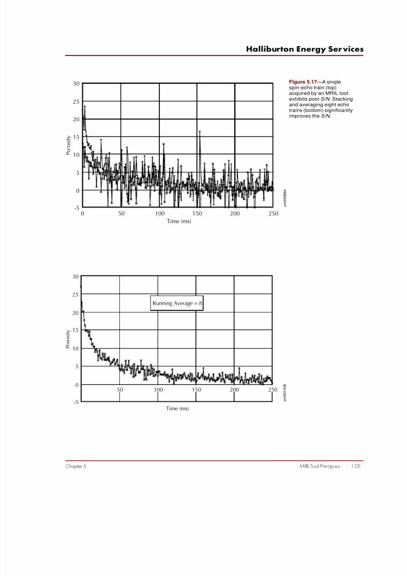
7/28/2019 NMR Logging Principles and Applications
http://slidepdf.com/reader/full/nmr-logging-principles-and-applications 123/253
MRIL Tool Principles 105
Halliburton Energy Services
Chapter 5
Figure 5.17 —A singlespin-echo train (top)acquired by an MRIL tool
exhibits poorS/N
. Stackingand averaging eight echotrains (bottom) significantlyimproves the S/N .
-5
0
5
10
15
20
25
30
Porosity
Time (ms)
50 100 150 200 250
Running Average = 8
0-5
50 100 150 200 250
0
5
10
15
20
25
30
Porosity
Time (ms)
o m
0 0 0 8 9 4
o m
0 0 1 4 3 6
7/28/2019 NMR Logging Principles and Applications
http://slidepdf.com/reader/full/nmr-logging-principles-and-applications 124/253
NMR Logging Principles and Applications
106 MRIL Tool Principles Chapter 5
• the number of operating frequencies used by the tool
- one frequency (Use an activation that employs one frequency.)
- two frequencies (Use an activation that employs two frequencies.)
- three frequencies (Use an activation that employs three frequencies.)
Each activation contains several parameters that must be chosen carefully to obtain accurate
data without exceeding the operational limits of the tool. Some of these parameters are
• polarization or wait time (TW )
• echo spacing (TE )
• number of echoes ( NE )
• running average ( RA)
Activation sets are tool-dependent. The actual choice of proper activations for an MRIL job
is a part of job planning, which is discussed in Chapter 8.
The nine frequencies of the MRIL-Prime tool allow it to obtain more data in a particular period than if only one frequency were used. Fig. 5.18 illustrates the application of these frequencies,7
which are selected from five bands, designated as bands 0, 1, 2, 3, and 4. A frequency chosen
from band 4 can be used to measure clay-bound water with a partial-polarization activation in
single-frequency mode. Frequencies from the other four bands can be used to run different
activation sets, such as standard T 2, dual TW , and/or dual TE , in dual-frequency mode. Fig. 5.19
shows the five frequency bands and their typical center frequencies.
Fig. 5.18 also illustrates the concept of measurement efficiency, [ XF x( NE xTE )]/TW , under
the assumption NE xTE = 500 ms and TW = 12 s, where XF is the number of frequencies used
and NE xTE is the pulse time. Measurement efficiency is thus only 4% for a single-frequency
measurement but 36% for a nine-frequency measurement.
Fig. 5.20 contains a simplified timing diagram for a dual-TW activation for the MRIL-Prime
tool.6 The activation initiates three different CPMG pulse sequences at various operating
frequencies:• For the first sequence, TE = 1.2 ms and TW = 12 s.
• For the second sequence, TE = 1.2 ms and TW = 1 s.
• For the third sequence, TE = 0.6 ms and TW = 0.02 s.
The cycle repeats every 14 s. At a logging speed of 1,000 ft/hr (16.7 ft/min), two samples per
foot are produced for each TW of 1 and 12 s in frequency bands 3, 2, 1, and 0, and one
sample per foot is produced for the TE of 0.6 ms in frequency band 4.
MRIL-Prime 6-in. sondes are equipped with additional pairs of magnets located above and
below the main magnet to achieve accelerated pre-polarization by their higher magnetic
fields.6 The main magnet is three times longer than the antenna aperture, which allows for
proper recovery from the higher polarization. At stationary or slow logging conditions, these
magnets offer no advantage, but at normal- or high-logging speeds, they effectively halve thetime needed for complete polarization, as shown in Fig. 5.21.

7/28/2019 NMR Logging Principles and Applications
http://slidepdf.com/reader/full/nmr-logging-principles-and-applications 125/253
MRIL Tool Principles 107
Halliburton Energy Services
Chapter 5
Fig. 5.18 —The ninefrequencies of the MRIL-Prime tool are selected
from five bands. Whenpolarization time is 12,000ms and pulse time is 500ms, the nine frequencies
give an efficiency of 36%compared to the 4%efficiency obtainable with
a single frequency.
Fig. 5.19 —Typical center-frequencies of the fiveMRIL frequency bands are
590, 620, 650, 680, and
760 kHz.
500 ms 12,000 ms 500 ms
4% Efficiency
Single Frequency
Time
36% Efficiency
Frequency Band 4
Frequency Band 3
Frequency Band 2
Frequency Band 1
Frequency Band 0
Multi-Frequency
o m
0 0 0 8 9 5
o m
0 0 0 8 9 6
BB
AA
AA
BB
C C C C
AA
BB
BB
AA
X
A CPMG Sequence: = 1.2 ms, = 12 s, = 400.TE TW NE
X X X
B CPMG Sequence: = 1.2 ms, = 1 s, = 400.TE TW NE C CPMG Sequence: = 0.6 ms, = 0.02 s, = 10. (Repeated 24Times)TE TW NE X Data Transfer
Legend:
Time-> .5 .5 .5 .5 .5 1.0 .5 .5 .5 .5 .5 1.0 .5 .5 .5 .5 .5 1.0 .5 .5 .5 .5 1.0 s.5Band
4
33221100
Figure 5.20 —This timingdiagram for a dual-TW
activation for an MRIL-Prime tool shows thatthree different CPMG
sequences are usedrepeatedly, two of themat various operatingfrequencies.
o m
0 0 0 8 9 7

7/28/2019 NMR Logging Principles and Applications
http://slidepdf.com/reader/full/nmr-logging-principles-and-applications 126/253
NMR Logging Principles and Applications
108 MRIL Tool Principles Chapter 5
Tool Configuration
In basic configuration, an MRIL tool consists of a magnetic mandrel with a diameter of 4 1/2,
4 7/8, or 6 in.; an electronics cartridge; and one or two energy-storage cartridges (capacitors),
as illustrated in Fig. 5.22. A fluid excluder, centralizers, and standoffs are optional items but
are always recommended and must be selected according to hole size.
The use of a fluid excluder reduces the loading effect of mud and increases the signal-to-
noise ratio. Centralizers and standoffs both help centralize the tool in the borehole. Further-
more, standoffs may protect the tool’s fiberglass body by keeping it away from the casing/ borehole wall.
MRIL tools are fully combinable with Halliburton’s other openhole logging tools, such as the
High-Resolution Array Induction (HRAI) tool, the Electrical Micro Imaging (EMI) tool, and
the Circumferential Acoustic Scanning Tool (CAST-V).
References
1. Taicher, Z., et al., 1986, Nuclear magnetic resonance sensing apparatus and techniques,
U.S. patent 4,717,877.
2. Taicher, Z., and Shtrikman, S., 1986, Nuclear magnetic resonance sensing apparatus and
techniques, U.S. patent 4,717,878.
3. Miller, M.N., et al., 1990, Spin-echo magnetic-resonance logging—porosity and free-fluid index, SPE 20561, 1990 SPE Annual Technical Conference and Exhibition Proceedings,
v.Ω (Formation evaluation and reservoir geology), p. 321–334.
4. Coates, G.R., et al., 1993, Restrictive diffusion from uniform gradient NMR well logging,
SPE 26472, 1993 SPE Annual Technical Conference and Exhibition Proceedings, v.Ω
(Formation evaluation and reservoir geology), p. 575–590.
Fig. 5.21 —These threecurves (left) show how fastmagnetization can be
achieved without acceler-ated pre-polarization. Thecurves correspond to T
1=
1, 2, and 4 s. If 5% under-
polarization can betolerated, 12 s are neededto polarize the slowest
component. With acceler-ated polarization as usedin the MRIL-Prime 6-in.
sonde (right), magnetiza-tion can be achieved morequickly. The most criticalcase of logging at 24 ft/min
is shown. The same T 1
distribution of 1, 2, and 4 sas was studied in the left
graph is assumed. After
6 s, all components havestabilized within a ± 5%band of the nominal
magnetization.
o m
0 0 0 8 9 8

7/28/2019 NMR Logging Principles and Applications
http://slidepdf.com/reader/full/nmr-logging-principles-and-applications 127/253
MRIL Tool Principles 109
Halliburton Energy Services
Chapter 5
Figure 5.22 —In its basic
configuration, the MRILtool consists of a magnetic
mandrel, an electronicscartridge, and one or two
energy-storage cartridges.
o m
0 0 1 6 0 9
Telemetry
EnergyCartridge
ElectronicCartridge
Standoff
Sonde
Cable Head
60"
161.5"
166”
166"
81"
Centralizer
Centralizer
Centralizer
Standoff
Mandrel

7/28/2019 NMR Logging Principles and Applications
http://slidepdf.com/reader/full/nmr-logging-principles-and-applications 128/253
NMR Logging Principles and Applications
110 MRIL Tool Principles Chapter 5
5. Chandler, R.N., et al., 1994, Improved log quality with a dual-frequency pulsed NMR
tool, SPE 28365, 1994 SPE Annual Technical Conference and Exhibition Proceedings,
v.Ω (Formation evaluation and reservoir geology), p. 23–35.
6. Prammer, M.G., et al., 1999, Theory and operation of a new, multi-volume, NMR logging
system, paper DD, 40th Annual SPWLA Logging Symposium Transactions, 12 p.
7. Prammer, M.G., et al., 1998, A new multiband generation of NMR logging tools,
SPE 49011, 1998 SPE Annual Technical Conference and Exhibition Proceedings, v.Ω
(Formation evaluation and reservoir geology), p. 237–243.
8. Prammer, M.G., et al., 1996, Measurements of clay-bound water and total porosity by
magnetic resonance logging, SPE 36522, 1996 SPE Annual Technical Conference and
Exhibition Proceedings, v.Ω (Formation evaluation and reservoir geology), p. 111–118.
Also published in 1996 in The Log Analyst , v. 37, no. 5, p. 61–69.
Additional information on NMR logging tool principles can be found in
following literature.
Akkurt R., 1990, Effects of Motion in Pulsed NMR Logging , Colorado School of Mines,
Golden, Colorado, unpublished Ph.D. dissertation, 165 p.
Allen, D., et al., 1997, How to use borehole nuclear magnetic resonance, Oilfield Review, v.,
9, no. 2, p. 2–15.
Brown, J.A., Brown, L.F., and Jackson, J.A., 1981, NMR (nuclear magnetic resonance)
measurements on western gas sands core, SPE/DOE 9861, 1981 SPE/DOE Low Perme-
ability Gas Reservoirs Symposium Proceedings, p. 321-326. Also published in 1981 as
Los Alamos National Laboratory Report No. LA-UR-81-736, 16 p.
Brown, J.A., et al., 1982, NMR Logging Tool Development—Laboratory Studies of Tight
Gas Sands and Artificial Porous Material, Los Alamos National Laboratory Report No.
LA-UR-82-447, 20 p. Also published in 1982 as SPE 10813 in 1982 SPE/DOE Uncon-
ventional Gas Recovery Symposium Proceedings, p. 203–209.
Brown, J.A., Jackson, J.A., and Koelle, A.R., 1985, Western Gas Sands Project Los Alamos
NMR Well Logging Tool Development, Los Alamos National Laboratory Report
LA-10374-PR, 77 p.
Chandler, R., 1995, NML hardware history and MRIL, chapter 6, in Georgi, D.T., ed.,
Nuclear Magnetic Resonance Logging Short Course Notes, 36th Annual SPWLA Logging
Symposium, Paris, France, 12 p.
Edwards, C., 1997, Effects of tool design and logging speed on T2
NMR log data, paper RR,
38th Annual SPWLA Logging Symposium Transactions, 13 p.
Georgi, D.T., et al., 1995, Vertical resolution and signal-to-noise characteristics of nuclear
magnetic resonance imaging logs, paper OOO, in Georgi, D.T., ed., Nuclear Magnetic
Resonance Logging Short Course Notes, 36th Annual SPWLA Logging Symposium
Transactions, Paris, France, 12 p.Jackson, J.A., 1984, Nuclear magnetic resonance logging, The Log Analyst , v. 25, no. 5,
September-October, p. 16.

7/28/2019 NMR Logging Principles and Applications
http://slidepdf.com/reader/full/nmr-logging-principles-and-applications 129/253
MRIL Tool Principles 111
Halliburton Energy Services
Chapter 5
Jackson, J.A., Brown, J.A., and Crawford, T.R., 1981, Remote Characterization of Tight Gas
Formations with a New NMR Logging Tool: Los Alamos National Laboratory Report No.
LA-UR-81-735, 18 p. Also published in 1981 as SPE/DOE 9860, in 1981 SPE/DOE
Symposium on Low Permeability Gas Reservoirs Proceedings, p. 313–320.
Jackson, J.A., Brown, J.A., and Koelle, A.R., 1982, Western Gas Sands Project, Los Alamos
NMR (Nuclear Magnetic Resonance) Well Logging Tool Development, Progress Report,
April 1, 1980–September 30, 1981, Los Alamos National Laboratory Report No.
LA-9151-PR, 24 p. Also published in 1982 as U.S. Department of Energy Fossil Energy
Report No. DOE/BC/10018-20, 34 p.
Jackson, J.A., Brown, J.A., and Koelle, A.R., 1982, Western Gas Sands Project, Los Alamos
NMR (Nuclear Magnetic Resonance) Well Logging Tool Development, Progress Report,
October 1, 1981–September 30, 1982, Los Alamos National Laboratory Report.
Mardon, D., et al., 1995, Improved environmental corrections for MRIL pulsed NMR logs
run in high-salinity boreholes, paper DD, 36th Annual SPWLA Logging Symposium
Transactions, 12 p.
Morriss, C.E., et al., 1996, Operating guide for the Combinable Magnetic Resonance tool,
The Log Analyst , v. 37, no. 6, p. 53–60.
Xiao, L.Z., 1998, NMR Imaging Logging Principles and Applications (in Chinese), Science
Press, Beijing, 328 p.

7/28/2019 NMR Logging Principles and Applications
http://slidepdf.com/reader/full/nmr-logging-principles-and-applications 130/253
NMR Logging Principles and Applications
112 MRIL Tool Principles Chapter 5

7/28/2019 NMR Logging Principles and Applications
http://slidepdf.com/reader/full/nmr-logging-principles-and-applications 131/253
Answer Products Derived from MRIL Stand-Alone Analysis 113
Halliburton Energy Services
Chapter 6
Answer ProductsDerived fromMRIL Stand-
Alone Analysis
Chapter 6
NMR data can be analyzed independently or in combination with
conventional data. When NMR data are interpreted independently, they
can provide porosity and permeability as well as complete information
on fluid types and fluid saturation in the invaded zone. Two computer-
center models are available for stand-alone analysis of MRIL data, the
Time Domain Analysis (TDA) model and the Diffusion Analysis
(DIFAN) model. Another model called the Enhanced Diffusion Method
(EDM) can be implemented during data acquisition and provides
valuable information for viscous-oil detection. Complete descriptionsof these models and their applications are discussed in this chapter.
Time Domain Analysis
Concept
Time Domain Analysis (TDA)1–3 relies on the fact that different fluids
have different rates of polarization, or different T 1
relaxation times.
The T 1
of both gas and light oil (viscosity less than 5 cp) is normally
much longer than the T 1
of water. Time Domain Analysis provides
• fluid types in the flushed zone
• corrected MRIL porosity in gas reservoirs (Without this correc-
tion, MRIL data underestimates porosity because of the long T 1
and low hydrogen index of gas.)
• corrected MRIL porosity in light oils
• complete fluid-saturation analysis in the flushed zone using only
MRIL data
Principle
Differential Spectrum Method
TDA was an outgrowth of the Differential Spectrum Method
(DSM),4–6 which was developed as an earlier application of dual-TW logging. The DSM technique is used mostly to qualitatively investi-
gate the existence of gas in a formation. The basis of the technique is
represented in Fig. 6.1.

7/28/2019 NMR Logging Principles and Applications
http://slidepdf.com/reader/full/nmr-logging-principles-and-applications 132/253
NMR Logging Principles and Applications
114 Answer Products Derived from MRIL Stand-Alone Analysis Chapter 6
Figure 6.1—In theDifferential SpectrumMethod, the long-TW andshort-TW echo trains arefirst converted to T
2
distributions, and theresulting T 2
distributionsare subtracted fromone another.
M (t) P(i)
Raw Data: Echo Train A (Long )TW
Processing Result: Distribution BT 2
t
T 2Raw Data: Echo Train B (Short )TW t
M (t)
Processing Result: Distribution AT 2T 2
A - B in T 2 Domain
Differential Spectrum
Processing Result: DistributionT 2T 2
P(i)
P(i)
OilGas
o m 0 0 0 9 1 3
Time Domain Analysis
With TDA, the subtraction is performed in the ordinary time domain instead of the T 2
domain. The TDA method has two key advantages over the DSM.
• The difference between the two echo trains is calculated in the time domain, so the
difference is more robust. The difference is then transformed to a T 2
distribution.
• TDA provides better corrections for underpolarized hydrogen and for hydrogen-
index effects.
Fig. 6.2 illustrates the TDA principle. A complete mathematical derivation of the Time
Domain Analysis technique is presented in the chapter Appendix.
Data Acquisition
TDA data are acquired with dual-TW activation. Dual-TW logging acquires two NMR decay
curves by utilizing a long TW and a short TW with a single TE . A typical TW pair is 1 and 8 s,
with a TE of 0.9 or 1.2 ms. Some of the TW S/TW L pairs for the dual-TW logging activationswere introduced in Chapter 5.
Fig. 6.3 illustrates the principle of dual-TW logging. The top and middle sections show the
polarization and echo acquisition with a dual-frequency mode using frequencies f 1
and f 2. In
this illustration, the short-TW echo train is acquired in the f 1
shell, or f 1
sensitive volume,
while the formation is being polarized in the f 2
shell. Then a long-TW echo train is acquired in

7/28/2019 NMR Logging Principles and Applications
http://slidepdf.com/reader/full/nmr-logging-principles-and-applications 133/253
Answer Products Derived from MRIL Stand-Alone Analysis 115
Halliburton Energy Services
Chapter 6
Figure 6.2 —In TimeDomain Analysis, thelong- and short-TW echotrains are first subtracted,and the echo train
difference is converted toa T 2
distribution.
M (t)
Raw Data: Echo Train A (Long )TW t
Echo Train Differencet
M (t)
A - B inTime Domain
Differential Echo Train
Processing Result: DistributionT 2 T 2
P(i)
Raw Data: Echo Train B (Short )TW t
OilGas
M (t)
o m 0 0 1 2 4 1
Figure 6.3 —Dual-TW
logging acquires apartially polarized echotrain with a short TW
(upper section) and a fullypolarized echo train with along TW (middle section).T
2distributions corre-
sponding to the two echotrains are generated(bottom section).
Acquisition
TW long
Short TW
TW short
Water
Light Oil
Gas
Long TW
M0
0
f 2
Acquisition
M0
0
f 1
Porosity
Short TW Long TW
BrineOilGas
T 2 Relaxation Time (ms) T 2 Relaxation Time (ms)
0 1 10 100 1,000 0 1 10 100 1,000 o m 0 0 0 9 0 0
7/28/2019 NMR Logging Principles and Applications
http://slidepdf.com/reader/full/nmr-logging-principles-and-applications 134/253
NMR Logging Principles and Applications
116 Answer Products Derived from MRIL Stand-Alone Analysis Chapter 6
the f 2shell. The short TW is selected so that the protons in water are fully polarized, but so that
the protons of both gas and light oils are only partially polarized. During the long-TW cycle, all
the protons from the water are fully polarized, and the protons from the gas and light oil are
more completely polarized than during the short-TW cycle. The full polarization of the water
implies that the difference between the long-TW and short-TW measurements is due to the gasand light oil signals. The bottom section in Fig. 6.3 shows the T
2distributions from both
echo trains.
Dual-TW logging results at the wellsite include short-TW and long-TW T 2
distributions; apparent
MPHI , BVI , and MFFI from both the short-TW and long-TW echo trains; and MPERM from the
long-TW measurements. Fig. 6.4 shows a dual-TW log. By comparing the BVI and MFFI from
both the short- and long-TW measurements, useful quick look information may be obtained.
Both gas and light oil have a long T 1, and thus need a longer TW for full polarization. If light
oil is present, the MFFI from the long TW will be greater than that from the short TW . In a gas
zone, the BVI and MFFI from long TW will be greater than that from the short TW .
Applications
Example 1Two wells from a field in Egypt show the importance of TDA in overcoming the effect of
underpolarization of light hydrocarbons to provide correct formation porosity. In the subject
field, the operator used a light oil-based mud, which has a T 1
value of about 5 s. Originally, the
effect of the light oil-based mud was not taken into consideration, which resulted in underesti-
mating the formation porosity. A comparison between core porosity and MRIL porosity on the
first well is shown in Fig. 6.5 and illustrates this underestimation as does a comparison between
the neutron-density crossplot porosity and MRIL porosity shown in Fig. 6.6.
In the second well, TDA was run to correct for the light oil-based mud in the invaded zone,
which affected the MRIL response because of the underpolarization of the hydrogen nuclei in
the mud. Fig. 6.7 compares core porosity with TDA-determined MPHI . Fig. 6.8 compares
neutron-density crossplot porosity with TDA-determined MPHI . The figures demonstrate that
TDA processing corrected the MPHI underestimation problem that was observed in the
previous well.
Example 2
Fig. 6.9 shows the result of applying TDA to the MRIL data of Fig. 6.4. Utilizing this tech-
nique, MRIL stand-alone analysis provides a complete solution for porosity, permeability and
fluid saturation in the flushed zone. According to the TDA results, a very good water-free pay
zone is located between XX685 and XX870 ft, although the resistivity is quite low from
XX715 to XX870 ft. A water zone is located from XX870 to XX880 ft.
As discussed before, the data acquired with NMR tools always contain noise, which results in
spectral broadening. The effects of spectral broadening when using the DSM can be severe
when the difference between hydrocarbon-filled porosity obtained from the two echo trains
(∆φh) is small.2 The signal may be smeared unequally into adjacent bins, and the differential
spectrum may appear to contain no hydrocarbon signal.
Example 3
A gas well drilled with oil-based mud in the Gulf of Mexico provides an example of complete
DSM and TDA processing.3 The logging program in the well consisted of logging-while-
drilling (LWD) gamma ray, resistivity, and neutron logs, and a wireline MRIL log. The MRIL

7/28/2019 NMR Logging Principles and Applications
http://slidepdf.com/reader/full/nmr-logging-principles-and-applications 135/253
Answer Products Derived from MRIL Stand-Alone Analysis 117
Halliburton Energy Services
Chapter 6
Figure 6.4 —This logshows dual-TW wellsiteresults. Track 1 contains aconventional gamma raycorrelation curve and long-
TW T 2 bin data. Track 2displays MPERM . Track 3displays the long-TW T
2
distribution. Track 4displays the short-TW T
2
distribution. Track 5contains the long-TW
MPHI and BVI curves.Track 6 contains the short-TW MPHI and BVI curves.
o m 0 0 1 6 1 0
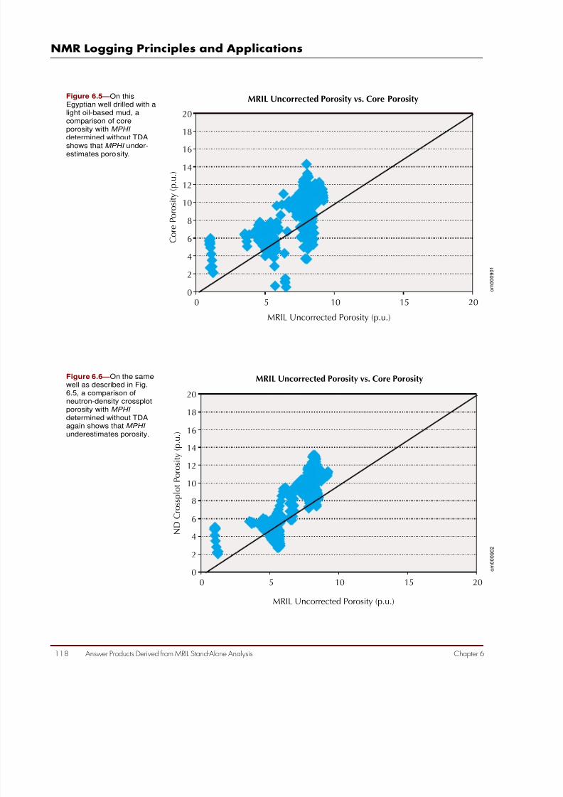
7/28/2019 NMR Logging Principles and Applications
http://slidepdf.com/reader/full/nmr-logging-principles-and-applications 136/253
NMR Logging Principles and Applications
118 Answer Products Derived from MRIL Stand-Alone Analysis Chapter 6
Figure 6.5 —On thisEgyptian well drilled with alight oil-based mud, acomparison of coreporosity with MPHI
determined without TDAshows that MPHI under-estimates porosity.
Figure 6.6 —On the samewell as described in Fig.6.5, a comparison ofneutron-density crossplotporosity with MPHI
determined without TDAagain shows that MPHI
underestimates porosity.
MRIL Uncorrected Porosity (p.u.)
CorePorosity(p.u.)
MRIL Uncorrected Porosity vs. Core Porosity
20
18
16
14
12
10
8
6
4
20
0 5 10 15 20
MRIL Uncorrected Porosity (p.u.)
ND
CrossplotPorosity(p.u.)
MRIL Uncorrected Porosity vs. Core Porosity
20
18
16
14
12
10
8
6
4
20
0 5 10 15 20
o m 0 0 0 9 0 1
o m 0 0 0 9 0 2
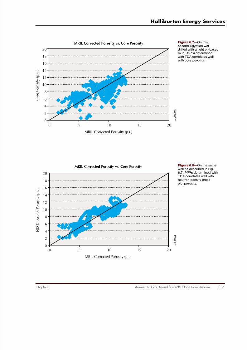
7/28/2019 NMR Logging Principles and Applications
http://slidepdf.com/reader/full/nmr-logging-principles-and-applications 137/253
Answer Products Derived from MRIL Stand-Alone Analysis 119
Halliburton Energy Services
Chapter 6
Figure 6.7 —On thissecond Egyptian welldrilled with a light oil-basedmud, MPHI determinedwith TDA correlates well
with core porosity.
Figure 6.8 —On the samewell as described in Fig.6.7, MPHI determined withTDA correlates well withneutron-density cross-
plot porosity.
CorePorosity(p.u.)
20
18
16
14
12
10
8
6
4
2
0
MRIL Corrected Porosity (p.u)
MRIL Corrected Porosity vs. Core Porosity
0 5 10 15 20
o m 0 0 0 9 0 3
o
m 0 0 0 9 0 4
MRIL Corrected Porosity (p.u)
ND
CrossplotPorosity(p.u.)
MRIL Corrected Porosity vs. Core Porosity
20
18
16
14
12
10
8
6
4
2
00 5 10 15 20

7/28/2019 NMR Logging Principles and Applications
http://slidepdf.com/reader/full/nmr-logging-principles-and-applications 138/253
NMR Logging Principles and Applications
120 Answer Products Derived from MRIL Stand-Alone Analysis Chapter 6
Figure 6.9 —TDA wasapplied to the MRIL dataof Fig. 6.4 to obtain theresults shown here. Track1 contains a conventional
gamma ray correlationcurve and long-TW T 2
bindata. Track 2 displaysMPERM and resistivitydata (both deep andshallow). Track 3 displaysthe long-TW T
2distribu-
tion. Track 4 displays thedifferential spectrum(imaging). Track 5contains TDA products:corrected effectiveporosity, BVI , and gas, aswell as oil and movable-water porosity.
o m 0 0 1 6 1 1
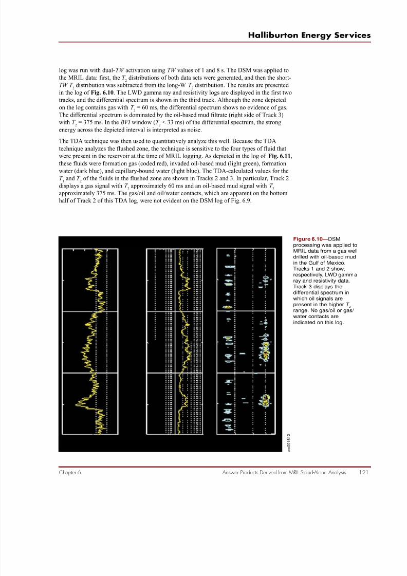
7/28/2019 NMR Logging Principles and Applications
http://slidepdf.com/reader/full/nmr-logging-principles-and-applications 139/253
Answer Products Derived from MRIL Stand-Alone Analysis 121
Halliburton Energy Services
Chapter 6
log was run with dual-TW activation using TW values of 1 and 8 s. The DSM was applied to
the MRIL data: first, the T 2
distributions of both data sets were generated, and then the short-
TW T 2
distribution was subtracted from the long-W T 2
distribution. The results are presented
in the log of Fig. 6.10. The LWD gamma ray and resistivity logs are displayed in the first two
tracks, and the differential spectrum is shown in the third track. Although the zone depicted on the log contains gas with T
2= 60 ms, the differential spectrum shows no evidence of gas.
The differential spectrum is dominated by the oil-based mud filtrate (right side of Track 3)
with T 2
= 375 ms. In the BVI window (T 2
< 33 ms) of the differential spectrum, the strong
energy across the depicted interval is interpreted as noise.
The TDA technique was then used to quantitatively analyze this well. Because the TDA
technique analyzes the flushed zone, the technique is sensitive to the four types of fluid that
were present in the reservoir at the time of MRIL logging. As depicted in the log of Fig. 6.11,
these fluids were formation gas (coded red), invaded oil-based mud (light green), formation
water (dark blue), and capillary-bound water (light blue). The TDA-calculated values for the
T 1
and T 2
of the fluids in the flushed zone are shown in Tracks 2 and 3. In particular, Track 2
displays a gas signal with T 2
approximately 60 ms and an oil-based mud signal with T 2
approximately 375 ms. The gas/oil and oil/water contacts, which are apparent on the bottom
half of Track 2 of this TDA log, were not evident on the DSM log of Fig. 6.9.
Figure 6.10 —DSMprocessing was applied toMRIL data from a gas welldrilled with oil-based mudin the Gulf of Mexico.Tracks 1 and 2 show,respectively, LWD gammaray and resistivity data.Track 3 displays thedifferential spectrum inwhich oil signals are
present in the higher T 2range. No gas/oil or gas/ water contacts areindicated on this log.
o m 0 0 1 6 1 2
GR Resistivity Differential Spectrum
20 120 0.1 10 1 10 100 1000

7/28/2019 NMR Logging Principles and Applications
http://slidepdf.com/reader/full/nmr-logging-principles-and-applications 140/253
NMR Logging Principles and Applications
122 Answer Products Derived from MRIL Stand-Alone Analysis Chapter 6
Diffusion Analysis
Concept
Diffusion Analysis depends on the diffusion contrast between fluids to type and quantify oils
with viscosities ranging between 0.5 to 35 cp at temperatures and pressures of at least 200 °F
and at least 2,000 psi. As discussed in Chapter 3, the diffusion relaxation mechanism occurs
because of the gradient of the MRIL magnetic field. The observed T 2 of a fluid changes withchanges in the echo spacing TE .7 The value of T 2depends on the magnetic field gradient G ,
the gyroscopic constant γ of the hydrogen nuclei, the echo spacing TE , and the apparent
diffusion coefficient Da
according to
( )[ ]12112
int22TE G DC T T
aγ += (6.1)
Figure 6.11 —TDA wasperformed on MRIL datafrom the well described inFig. 6.10. Track 1 showsthe pore volumes for gas
(red), oil-based mudfiltrate and/or native oil(green), movable water(dark blue), and capillary-bound water (light blue)obtained from TDAquantitative analysis.Tracks 2 and 3 show,respectively, the T
2and T
1
values of gas and light oilcalculated through TDA. Ahydrocarbon signal with anunclear origin (yellow)appears in Track 2. Thelower part of Track 2shows oil/water and gas/ oil contacts, while the
upper part of the trackindicates the presence ofgas and oil.
o m 0 0 1 6 1 3

7/28/2019 NMR Logging Principles and Applications
http://slidepdf.com/reader/full/nmr-logging-principles-and-applications 141/253
Answer Products Derived from MRIL Stand-Alone Analysis 123
Halliburton Energy Services
Chapter 6
where T 2int
is the intrinsic relaxation time when the field gradient is zero. C accounts for the
combined effects of restricted diffusion and spin dynamics associated with the mixing of
direct and stimulated echoes in a gradient magnetic field. 8 For the MRIL tool, C = 1.08. For a
given job, all the parameters in Eq. 6.1 are constants except for the echo spacing TE . Eq. 6.1
shows that increasing the echo spacing from 1.2 ms to a higher value will generate a lower T
2value.
Data Acquisition
Diffusion analysis requires echo data from a dual-TE activation.9 Dual-TE logging acquires
two types of CPMG echo trains by utilizing a short and a long TE with a single TW . For full
polarization, TW should be at least three times the maximum T 1
of all pore fluids. A typical
TE pair is 1.2 and 4.8 ms.
The dual-TE activation allows the principle of diffusion-weighted measurements to be
applied to distinguish water from medium-viscosity oil. The oil must have a significantly
smaller Da
than the water, and in practice, the oil viscosities must range approximately
from 0.5 to 35 cp. Through comparison of the CPMG echo trains derived from the shortecho spacing (TE S) and long echo spacing (TE
L), the oil signal is distinguished from the
water signal.
Fig. 6.12 illustrates the principle of dual-TE logging. The top and middle sections show the
polarization and echo acquisition using a dual-frequency mode with frequencies f 1
and f 2.
While the f 2
shell is being re-polarized, data is acquired in the f 1
shell. The process then
reverses. In this illustration, a long TE echo train is acquired in the f 1
shell, and a short TE
echo train is acquired in the f 2
shell. For the long-TE measurement, the decay of the water
signal is much faster than the decay of the medium-viscosity-oil signal. By careful selection
Figure 6.12 —Dual-TE
logging acquires two fullypolarized echo trains, one
from a long-TE measure-ment (top) and the otherfrom a short-TE measure-ment (middle). Theresulting T
2distributions
(bottom) can be used todistinguish water from oil.
Polarization
Polarization
M 0
M 0
0
0
Porosity
f 1
f 2
Long TE
Short TE
Short TE BrineOil
0
T 2 Relaxation Time (ms)
0
T 2 Relaxation Time (ms)
G as
L igh t oil
G as
Acquisition
Acquisition
1 10 100 1,0001 10 100 1,000
Long TE
o m 0 0 0 9 0 5

7/28/2019 NMR Logging Principles and Applications
http://slidepdf.com/reader/full/nmr-logging-principles-and-applications 142/253
NMR Logging Principles and Applications
124 Answer Products Derived from MRIL Stand-Alone Analysis Chapter 6
of the long TE , the signals from water and oils can be separated. For the short-TE measure-
ment, the water T 2
distribution overlaps much of the oil T 2
distribution. The bottom section
shows T 2
distributions from both echo trains.
At the wellsite, products from dual-TE logging include two T 2
distributions, MPHI and BVI
from both the short-TE and long-TE echo trains, and MPERM from the short-TE measure-ments, as shown in Fig. 6.13. (The log in this figure was calculated with the default param-
eters T 2cutoff
= 33 ms and C = 10, where C is the Coates-model coefficient.) Later results may
differ from the wellsite results because of subsequent refinements in measurement parameters
and computational assumptions. For example, both the polarization time TW and the hydro-
gen index HI will affect MPHI and BVI . Additionally, T 2cutoff
affects BVI and MFFI . MPERM
is affected by the same factors as BVI as well as by the Coates-model coefficient. From a
comparison of the T 2
distributions and of BVI and MFFI from both the short- and long-TE
measurements, useful quick look information may be obtained. Gas has a high diffusivity,
viscous oil has a low diffusivity, and the diffusivity of water is between the gas and viscous-
oil diffusivities. Therefore, gas, water, and viscous oil will exhibit different shifts on the T 2
distributions from the short-TE to the long-TE MRIL measurements.
Shifted Spectrum MethodThe Shifted Spectrum Method 4 (SSM) is a qualitative technique used to represent the
changes in the T 2
values of fluids, and hence changes in their T 2
distributions, when different
echo spacings are used. Consider a formation that contains fluids composed of water and
medium-viscosity oil. The diffusion coefficient for water is about 10 times larger than that for
the medium-viscosity oil. When TE is increased, the diffusion process will decrease the T 2
of
water more than the T 2
of oil. Long- and short-TE values (TE L
and TE S) can be selected so
that the reduction in water and oil T 2
values measured with TE L
relative to those measured
with TE S
can be used to separate the water signal from the oil signal. Comparison of the T 2
distributions determined with TE Land TE
Sdemonstrates the relative diffusion-induced shifts
of the water and oil T 2
values, which were seen in Chapters 1 and 4.
Quantitative Diffusion Analysis: DIFAN
DIFAN is an empirical model for quantitative diffusion analysis that has been used success-fully in many oil fields. It was developed to address problems where there is insufficient T
1
contrast to use the TDA method or too little diffusion contrast to use the more straightforward
dual-TE or EDM methods. It uses the different shifting of the T 2
values for different fluids
produced by the diffusion phenomenon to provide quantitative values of the water-filled and
hydrocarbon-filled porosity. For hydrocarbon liquids with very low viscosities, i.e., light oil
and condensates, DIFAN is not recommended because the differences between the diffusion
coefficients of hydrocarbons and water are too small. For high-viscosity oil (heavy oil),
DIFAN is also not recommended because the difference between the T 2int
values of dead oil
and irreducible water is too small.
The DIFAN model generates two T 2
distributions using the two echo trains generated from
dual-TE logging. The apparent T 2
geometric means of the free-fluid windows of the TE L
and
TE S T
2distributions are calculated and are designated as T
2Land T
2S, respectively. The two
means are then correlated to the diffusion parameters through the following two equations:
( )[ ]12112
int22S S aTE G DC T T γ += (6.2)
( )[ ]12112
int22L LaTE G DC T T γ += (6.3)

7/28/2019 NMR Logging Principles and Applications
http://slidepdf.com/reader/full/nmr-logging-principles-and-applications 143/253
Answer Products Derived from MRIL Stand-Alone Analysis 125
Halliburton Energy Services
Chapter 6
Figure 6.13 —This logshows dual-TE wellsiteproducts. Track 1 containsa conventional gamma raycorrelation curve and T
2
bin data from short-TE echo trains. Track 2 showsthe calculated MPERM .Track 3 displays the short-TE T
2distribution. Track 4
displays the long-TE T 2
distribution. Track 5contains the short-TE
MPHI and BVI curves.Track 6 contains the long-TE MPHI and BVI curves.
o m 0 0 1 6 1 4

7/28/2019 NMR Logging Principles and Applications
http://slidepdf.com/reader/full/nmr-logging-principles-and-applications 144/253
NMR Logging Principles and Applications
126 Answer Products Derived from MRIL Stand-Alone Analysis Chapter 6
where
T 2int
= intrinsic T 2
of the pore fluid (1/T 2int
= 1/T 2bulk
+ 1/T 2surface
)
Da
= apparent diffusion coefficient of the pore fluid
C = a constant that accounts for the combined effects of restricted
diffusion and spin dynamics associated with the mixing of direct
and stimulated echoes in a gradient magnetic field (1.08 for MRIL tools)
Because T 2S
, T 2L
, TE S, TE
L, G , γ , and C are known, the two equations can be solved simulta-
neously to obtain T 2int
and Da. The solution of the two equations is then used to construct a
crossplot between 1/T 2int
and Da/ D
was shown in Fig. 6.14, from which S
wais determined for
calculating Sw.
Before the points ( Da/ D
w,1/T
2int) are plotted, the S
wa= 100% and S
wa= 0% lines are con-
structed. For the construction, Dw, D
oil, and T
2bulk,oilmust be known.
Figure 6.14 —A 1/ T 2int vs.D
a / D
w crossplot, such as
shown here, is used inDIFAN analysis todetermine S
wa , from
which S w
is calculated.
o m 0 0 0 9 0 6
The S wa
= 100% line is the line that forms the upper boundary of the data points in a water-
saturated formation. This line passes through the bulk-water point ( Da/ D
w= 1). Empirical
results place the 1/T 2int intercept of this line at 0.04 ms -1, or T 2int = 25 ms. The exact location of this intercept is not critical for most hydrocarbon-bearing formations because changes in
saturation are primarily a function of Da/ D
w.
To determine the S wa
= 0% line, the formation is considered to be at irreducible water
conditions so that the free fluid is oil. T 2int
will then equal T 2bulk,oil
, and Da
will equal Doil
at

7/28/2019 NMR Logging Principles and Applications
http://slidepdf.com/reader/full/nmr-logging-principles-and-applications 145/253
Answer Products Derived from MRIL Stand-Alone Analysis 127
Halliburton Energy Services
Chapter 6
reservoir conditions. Thus, the point ( Doil
/ Dw,1/T
2bulk,oil) will be on the S
wa= 0% line, and the
line should be parallel to the S wa
= 100% line.
To map S wa
in the area between the 0% and the 100% S wa
lines, equally spaced lines that are
parallel to the 0% and 100% S wa
lines are constructed between the 0% and the 100% S wa
lines.
Thus, after T 2int
and Da
are calculated at a particular depth, the point ( Da/D
w, 1/T
2int) is plotted,
and S wa
is determined from the crossplot. S w
is subsequently calculated from
BVI FFI
BVI FFI S S
wa
w+
+= (6.4)
In summary, the process of diffusion analysis using fluid diffusion properties and the DIFANmodel is as follows:
1. Acquire two echo trains with dual-TE activation.
2. Estimate the bulk properties (T 2int
and D) of oil and water at reservoir conditions
(e.g., temperature, pressure, and oil viscosity).
3. Contruct the crossplot of 1/T 2int
vs. Da/ D
w.
4. Calculate the T 2 geometric means for the free-fluids window of the TE L and
TE S T
2distributions.
5. Calculate T 2int
and Da
from Eqs. 6.2 and 6.3.
6. Estimate S wa
by using the crossplot of 1/T 2int
vs. Da/ D
w.
7. Use S wa
to calculate true S w
in the effective porosity system.
Fig. 6.15 is one of the many successful DIFAN examples from Indonesia. The MRIL data
were acquired with dual-TE activation having TE S
= 1.2 ms and TE L
= 4.8 ms. The DIFAN
answer products in Track 5 show that the intervals from X95 to X20 ft, XX05 to XX00 ft,
and XX60 to XX30 ft are hydrocarbon zones with significant free water. Production data
confirmed these results.
Enhanced Diffusion Method
The Enhanced Diffusion Method 8, 10 (EDM) types and quantifies oils with viscosities ranging
between 1 and 50 cp. The EDM relies on diffusion contrasts to differentiate the fluids. Use of
a properly selected long TE enhances the diffusion effect during echo-data acquisition and
allows water and oil to be separated on a T 2
distribution generated from the logged data. The
EDM can use CPMG measurements acquired with the following activations:
• standard-T 2
logging with a long TE
• dual-TE logging with a single long TW
• dual-TW logging with a single long TE
An understanding of the EDM principle depends on an understanding of the factors affecting
the relaxation rates of water and oil in rock pores. If two echo trains are acquired during
dual-TE logging, the resulting TE L and TE S T 2 distributions will both include water and oilsignals. TE
Lcan be selected so that oil and water signals will separate on the TE
L T
2distribu-
tion, thereby providing a quick-look EDM result at the wellsite.
As discussed in Chapter 3, the relaxation rates of fluids in rock pores observed with CPMG
measurements are related to bulk, surface, and diffusion relaxation mechanisms:
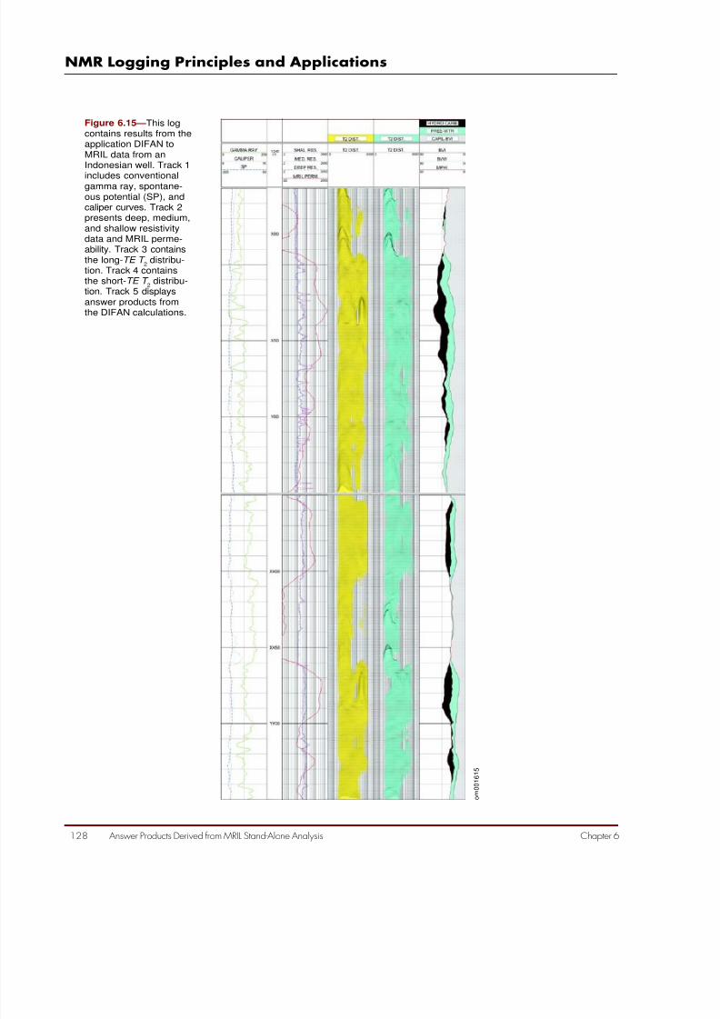
7/28/2019 NMR Logging Principles and Applications
http://slidepdf.com/reader/full/nmr-logging-principles-and-applications 146/253
NMR Logging Principles and Applications
128 Answer Products Derived from MRIL Stand-Alone Analysis Chapter 6
Figure 6.15 —This logcontains results from theapplication DIFAN toMRIL data from anIndonesian well. Track 1
includes conventionalgamma ray, spontane-ous potential (SP), andcaliper curves. Track 2presents deep, medium,and shallow resistivitydata and MRIL perme-ability. Track 3 containsthe long-TE T
2distribu-
tion. Track 4 containsthe short-TE T
2distribu-
tion. Track 5 displaysanswer products fromthe DIFAN calculations.
o m 0 0 1 6 1 5

7/28/2019 NMR Logging Principles and Applications
http://slidepdf.com/reader/full/nmr-logging-principles-and-applications 147/253
Answer Products Derived from MRIL Stand-Alone Analysis 129
Halliburton Energy Services
Chapter 6
diffusion2surface2 bulk 2CPMG21111 T T T T ++= (6.5)
The T 2
measured by a CPMG sequence is smaller than the T 2
calculated for any of the three
relaxation mechanisms. Because T 2bulk
is always much larger than T 2surface
and T 2diffusion
, T 2bulk
can
be ignored in practical applications. If T 2surface is smaller than T 2diffusion, then surface relaxationdominates the observed relaxation. Otherwise, diffusion relaxation dominates.
The diffusion effect can be manipulated to an extent by the choices of MRIL-tool operational
parameters. In particular, the strength of the field gradient G is a function of the operating
frequency and tool type, and the inter-echo spacing TE can be selected by the logging
engineer at the wellsite. G and TE can be chosen so that the diffusion mechanism dominates
water relaxation and thus so that the upper limit of T 2
for water in rock pores is T 2diffusion,w
. This
upper limit, designated T 2DW
, is given by
( )[ ]22
TE G DC 12T w DW
γ = (6.6)
Therefore, T 2DW
constitutes the absolute upper bound for the measured T 2
of water, and all T 2
relaxation times associated with water will be less than or equal to T 2DW.The T
2 of oil in water-wet rock pores is determined by both bulk and diffusion relaxation and
is given by
oil diffusion,oil bulk, T T T 22oil2 111 += (6.7)
The selection of TE and G can be often further refined so that
T 2DW
<< minimum T 2oil
values expected over the formation
(6.8)
In reality, because of noise effects, TE and G are usually selected so that
2T 2DW
<< minimum T 2oil
values expected over the formation (6.9)
Thus, the existence of a signal on the T 2
distribution longer than T 2DW
unambiguously indi-
cates the presence of oil in the formation. Fig. 6.16 shows how this observation is used to
recognize pay on EDM log displays.
The use of the EDM is quite straightforward. A T 1
contrast is not necessary, and depending on
oil NMR properties and the job objective, EDM data processing can be done in either T 2
domain or time domain. If the EDM objective is to discriminate pay from non-pay, then a
single CPMG measurement with long TW (for full polarization) and long TE (for diffusion
enhancement) is sufficient. Thus, standard-T 2
logging with a long TE can be used. If the EDM
objective is to quantify fluids in a pay zone, then dual-TE logging will be required. The short-
TE measurements will provide correct MPHI and BVI . If the T 2
contrast over the zone of
interest is not expected to be large enough to separate the T 2
values of water and oil, then
dual-TW logging with a single, long TE may be required to obtain data for TDA processing.
Thus, job planning is critical for EDM success.
Appendix: TDA Mathematical Model11
An understanding of how TDA determines the oil- and gas-filled porosity from the differen-
tial spectrum can be based on discussions in Chapter 3. In particular, Eq. 3.17 indicates that

7/28/2019 NMR Logging Principles and Applications
http://slidepdf.com/reader/full/nmr-logging-principles-and-applications 148/253
NMR Logging Principles and Applications
130 Answer Products Derived from MRIL Stand-Alone Analysis Chapter 6
Figure 6.16 —In this logdisplay, the T
2distributions
from TE = 1.2, 3.6, and 4.8ms are shown in Tracks 3,4, and 5 respectively. On
the EDM results in Track 4and 5, significant energyto the right of the T
2DWline
indicates obvious oilzones. Also note theincreased separation inTrack 5 because of theincreased TE .
the amplitude of an echo train acquired with a CPMG sequence for a water-wet rock satu-
rated with water, oil, and gas can be given by Eq. 6-A.1, when both oil and gas are assumed to have single T
2values.
M (t ) = Σ[ M 0iexp(-t /T
2i)] + M
oil exp(-t /T
2oil) + M
gasexp(-t/T
2gas) (6-A.1)
When polarization effects are considered, M0i, M
oil, and M
gascan be expressed as
M 0i = M
0i(0)[1- exp(-TW /T
1i)]
M oil
= M oil
(0)[1- exp(-TW /T 1oil
)]
M gas
= M gas
(0)[1- exp(-TW /T 1gas
)] (6-A.2)
The amplitudes of echo trains for TW L
and TW S
are then given as
M TW (t )=Σ M 0i(0)[1- exp(-TW L/T 1i)]exp(-t /T 2i)
+ M oil
(0)[1- exp(-TW L/T
1oil)]exp(-t /T
2oil)
+ M gas
(0)[1- exp(-TW L/T
1gas)]exp(-t /T
2gas) (6-A.3)
o m 0 0 1 6 1 6
L

7/28/2019 NMR Logging Principles and Applications
http://slidepdf.com/reader/full/nmr-logging-principles-and-applications 149/253
Answer Products Derived from MRIL Stand-Alone Analysis 131
Halliburton Energy Services
Chapter 6
and
M TW
(t )=Σ M 0i(0)[1- exp(-TW
S /T
1i)]exp(-t /T
2i)
+ M oil
(0)[1- exp(-TW S
/T 1oil
)]exp(-t /T 2oil
)
+ M gas
(0)[1- exp(-TW S /T
1gas)]exp(-t /T
2gas) (6-A.4)
∆ M (t )= M TWL
(t ) - M TWS
(t )
= Σ M 0i(0)exp(-t /T
2i) [exp(-TW
S /T
1i)- exp(-TW
L/T
1i)]
+ M oil
(0)exp(-t /T 2oil
) [exp(-TW S /T
1oil)- exp(-TW
L/T
1oil)]+
M gas
(0)exp(-t /T 2gas
)[exp(-TW S /T
1gas)- exp(-TW
L/T
1gas)] (6-A.5)
Polarization functions are then defined for water (∆αwi
), oil (∆αo), and gas (∆α
g ) as follows:
∆αwi
=[exp(-TW S /T
1i)- exp(-TW
L/T
1i)] (6-A.6)
∆αo=[exp(-TW
S /T
1oil)- exp(-TW
L/T
1oil)] (6-A.7)
∆α g
=[exp(-TW S /T
1gas)- exp(-TW
L/T
1gas)] (6-A.8)
Eq. 6-A.5 subsequently becomes
∆ M (t ) =Σ[ M 0i(0)exp(-t /T
2i) ∆α
wi ]+ M
oil(0)exp(-t /T
2oil) ∆α
o + M
gas(0)exp(-t /T
2gas) ∆α
g
(6-A.9)
If TW S
was selected to fully polarize the protons of water in rock pores, then ∆αwi
≅ 0. This
condition allows the difference of the two echo trains to be written as
∆M(t ) = M oil
(0)exp(-t /T 2oil
) ∆αo
+ M gas
(0)exp(-t /T 2gas
) ∆α g
(6-A.10)
A differential porosity function is then defined by
∆φ(t ) = φ*oil
exp(-t /T 2oil
) + φ*gas
exp(-t /T 2gas
) + noise (6-A.11)
where
noise = noise during CPMG measurement of the two echo trains
∆φ = difference in hydrocarbon-filled porosity obtained from the echo trains
φ∗oil = apparent oil-filled porosity obtained from the difference of the twoecho trains
φ∗gas
= apparent gas-filled porosity obtained from the difference of the two
echo trains
S

7/28/2019 NMR Logging Principles and Applications
http://slidepdf.com/reader/full/nmr-logging-principles-and-applications 150/253
NMR Logging Principles and Applications
132 Answer Products Derived from MRIL Stand-Alone Analysis Chapter 6
Finally, the apparent porosities are related to the true porosities (φoil
and φgas
) by
φ*oil
= [ M oil
(0)/ M 100%
(0)] ∆αo= φ
oil HI
oil∆α
o(6-A.12)
φ*gas
= [ M gas
(0)/ M 100%
(0)] ∆α g
= φgas
HI gas∆α
g (6-A.13)
where
M 100%
(0) = amplitude of CPMG echo train at time zero obtained from an MRIL water-
tank (i.e., 100% porosity) calibration
HI oil
= hydrogen index of oil
HI gas
= hydrogen index of gas
Therefore,
• If the values of T 2oil
and T 2gas
are known at reservoir conditions, then Eq. 6-A.11 can be
used to calculate the apparent porosities, φ*oil
and φ*gas
.
• If the values of T 1oil
, T 1gas
, HI oil
, and HI gas
are also known, then Eqs. 6-A.12 and 6-A.13
can be used to calculate the true porosities, φoil
and φgas
.
The actual TDA procedure includes the following steps:
1. Acquire two echo trains with dual-TW activation.
2. Estimate the bulk properties (T 1, T
2, and HI ) of oil and gas at reservoir conditions (e.g.,
temperature, pressure, and oil viscosity).
3. Subtract the echo trains from one another.
4. Search T 2
for gas and oil, and search T 1
for oil at reservoir conditions.
5. Calculate the apparent porosities (φ*oil
and φ*gas
) using Eq. 6-A.11.
6. Calculate the true porosities (φoil
and φgas
) using Eqs. 6-A.12 and 6-A.13, the bulk
properties estimated in Step 2, and the apparent porosities found in Step 5. (Note that
the T 1
values estimated in Step 2 or measured by a triple-TW 12 activation are used to
calculate the oil and gas polarization functions.)
7. Calculate water porosity and effective porosity.
The following summarizes several TDA assumptions that were discussed earlier in this
appendix:
• In Eq. 6-A.1, each of the oil and gas signals exhibits a single-exponential decay. This
single-exponential decay is a reasonable approximation for the decay of gas and manylow-viscosity oils.
• In Eq. 6-A.10, TW S
should be selected so that the water protons are fully polarized.
Otherwise, a water-polarization correction is needed, and the analysis process will be
more complicated.
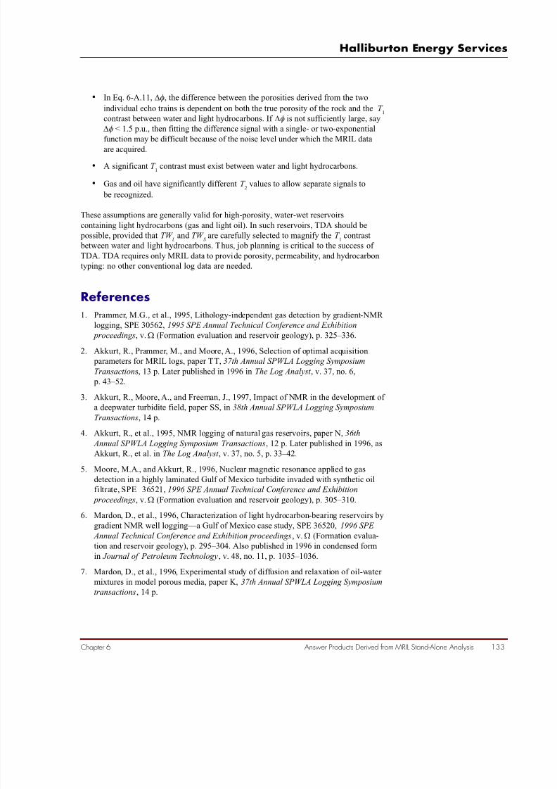
7/28/2019 NMR Logging Principles and Applications
http://slidepdf.com/reader/full/nmr-logging-principles-and-applications 151/253
Answer Products Derived from MRIL Stand-Alone Analysis 133
Halliburton Energy Services
Chapter 6
• In Eq. 6-A.11, ∆φ, the difference between the porosities derived from the two
individual echo trains is dependent on both the true porosity of the rock and the T 1
contrast between water and light hydrocarbons. If ∆φ is not sufficiently large, say
∆φ < 1.5 p.u., then fitting the difference signal with a single- or two-exponential
function may be difficult because of the noise level under which the MRIL dataare acquired.
• A significant T 1 contrast must exist between water and light hydrocarbons.
• Gas and oil have significantly different T 2
values to allow separate signals to
be recognized.
These assumptions are generally valid for high-porosity, water-wet reservoirs
containing light hydrocarbons (gas and light oil). In such reservoirs, TDA should be
possible, provided that TW L
and TW S
are carefully selected to magnify the T 1
contrast
between water and light hydrocarbons. Thus, job planning is critical to the success of
TDA. TDA requires only MRIL data to provide porosity, permeability, and hydrocarbon
typing: no other conventional log data are needed.
References
1. Prammer, M.G., et al., 1995, Lithology-independent gas detection by gradient-NMR
logging, SPE 30562, 1995 SPE Annual Technical Conference and Exhibition
proceedings, v.Ω (Formation evaluation and reservoir geology), p. 325–336.
2. Akkurt, R., Prammer, M., and Moore, A., 1996, Selection of optimal acquisition
parameters for MRIL logs, paper TT, 37th Annual SPWLA Logging Symposium
Transactions, 13 p. Later published in 1996 in The Log Analyst , v. 37, no. 6,
p. 43–52.
3. Akkurt, R., Moore, A., and Freeman, J., 1997, Impact of NMR in the development of
a deepwater turbidite field, paper SS, in 38th Annual SPWLA Logging Symposium
Transactions, 14 p.
4. Akkurt, R., et al., 1995, NMR logging of natural gas reservoirs, paper N, 36th
Annual SPWLA Logging Symposium Transactions, 12 p. Later published in 1996, as
Akkurt, R., et al. in The Log Analyst , v. 37, no. 5, p. 33–42.
5. Moore, M.A., and Akkurt, R., 1996, Nuclear magnetic resonance applied to gas
detection in a highly laminated Gulf of Mexico turbidite invaded with synthetic oil
filtrate, SPE 36521, 1996 SPE Annual Technical Conference and Exhibition
proceedings, v.Ω (Formation evaluation and reservoir geology), p. 305–310.
6. Mardon, D., et al., 1996, Characterization of light hydrocarbon-bearing reservoirs by
gradient NMR well logging—a Gulf of Mexico case study, SPE 36520, 1996 SPE
Annual Technical Conference and Exhibition proceedings, v.Ω (Formation evalua-
tion and reservoir geology), p. 295–304. Also published in 1996 in condensed form
in Journal of Petroleum Technology, v. 48, no. 11, p. 1035–1036.
7. Mardon, D., et al., 1996, Experimental study of diffusion and relaxation of oil-water
mixtures in model porous media, paper K, 37th Annual SPWLA Logging Symposium
transactions, 14 p.

7/28/2019 NMR Logging Principles and Applications
http://slidepdf.com/reader/full/nmr-logging-principles-and-applications 152/253
NMR Logging Principles and Applications
134 Answer Products Derived from MRIL Stand-Alone Analysis Chapter 6
8. Akkurt, R., et al., 1998, Enhanced diffusion: expanding the range of NMR direct
hydrocarbon-typing applications, paper GG, 39th Annual SPWLA Logging Symposium
Transactions.
9. Mardon, D., Prammer, M.G., and Coates, G.R., 1996, Characterization of light hydrocarbon
reservoirs by gradient-NMR well logging, Magnetic Resonance Imaging , v. 14,
nos. 7 and 8, p. 769–777.
10. Akkurt, R., et al., 1998, Determination of Residual Oil Saturation Using Enhanced
Diffusion, SPE 49014.
11. Xiao, L.Z., 1998, NMR imaging logging principles and applications (in Chinese),
Science Press, Beijing. 328 p.
12. Hou, L., et al., 1999, Enhanced NMR logging methods for accurately measuring volumes
of gas and light oil in hydrocarbon reservoirs, SPE 56769, prepublication print, 14 p.
7/28/2019 NMR Logging Principles and Applications
http://slidepdf.com/reader/full/nmr-logging-principles-and-applications 153/253
Answer Products Derived from MRIL Combinations with Other Logs 135
Halliburton Energy Services
Chapter 7
Answer ProductsDerived fromMRILCombinations
with Other Logs
Chapter 7
As stated in Chapter 6, MRIL stand-alone analysis, such as Time
Domain Analysis and Diffusion Analysis, provides interpretation of the
invaded zone because of the shallow depth of investigation of MRIL
measurements. If MRIL data are combined with other logs, analysis
can furnish even more information about the reservoir. For example, a
combination of MRIL and deep-resistivity data provides a complete
analysis of the fluids in the virgin zone. MRIAN is one of the interpre-
tation models that uses this data combination.1 This chapter contains a
complete discussion of MRIAN and its applications.
If MRIL data are combined with quad-combo data (neutron, density,
sonic, and resistivity), then the combination can provide critical
information for well completions. For example, when used in a model
called StiMRILTM, such data can generate information about rock
properties, formation lithology, and formation permeability. The
StiMRIL model and its application in stimulation optimization are
discussed in this chapter.
MRIAN Concept
MRIAN combines MRIL data and the deep-resistivity data from lateral
or induction logs. MRIAN uses the dual-water model2
to provide thevolume of formation fluids in the virgin zone. The main data require-
ments for MRIAN processing are true formation resistivity ( Rt ), total
porosity (φT ), and clay-bound-water saturation (S
wb). MRIL data are
used to provide two important parameters needed in the dual-water
model: the clay-bound water porosity ( MCBW ) and effective porosity
( MPHI ). A similar analysis could be implemented with different
resistivity models, such as Archie or Waxman-Smits.3
MRIAN Principles
Dual-Water Model
The Dual-water model is illustrated in the left panel of Fig. 7.1 and can be expressed mathematically by
( )
+
−=
wT
wb
cw
wT
wb
w
n
wT
m
T t S
S C
S
S C S C 1φ
(7.1)

7/28/2019 NMR Logging Principles and Applications
http://slidepdf.com/reader/full/nmr-logging-principles-and-applications 154/253
NMR Logging Principles and Applications
136 Answer Products Derived from MRIL Combinations with Other Logs Chapter 7
where
C t
= formation conductivity
C w
= conductivity of formation water
C cw
= conductivity of clay-bound water
φT
= total porosity (includes free fluids, capillary-bound water, and
clay-bound water)
S wT
= total water saturation (as a fraction of total porosity)
S wb
= clay-bound-water saturation (as a fraction of total porosity)
m = cementation exponent
n = saturation exponent
C cw
is temperature-dependent and is given by
C cw
= 0.000216 (T - 16.7)(T + 504.4) (7.2)
where T is formation temperature in degrees Fahrenheit.
Coates modified the dual-water model to reduce the uncertainty of the exponents m and n by
introducing a parameter W defined by
( )( )
wT T
n
wT
m
T
S
S W
φ
φ
log
log= (7.3)
Figure 7.1— The dual-watermodel (left panel) providesa more comprehensivedescription of pore fluids forshaly formations than doesthe Archie model (rightpanel), which is applicablein clean formations. MRILresponses (middle panel) inthis application provide twoimportant parametersneeded in MRIAN imple-mentation of the dual-watermodel: clay-bound waterporosity (MCBW ) andeffective porosity (MPHI ).
o m 0 0 0 9 0 7
Shaly Formation Formation Clean Formation
Dual-water Model MRIL Response Archie Model
Matrix Solids
Clay-bound Water Clay-bound Water
Capillary-bound Water Capillary-bound Water
Capillary-boundWater
Free Water Free Water
Hydrocarbon Hydrocarbon
MCBW
Dry Clay
Matrix
FreeWater
Hydrocarbon
FFI MPHI
Solid
BVI
Liquid
V sh
T φ
e φ
hφ hφ
w φ
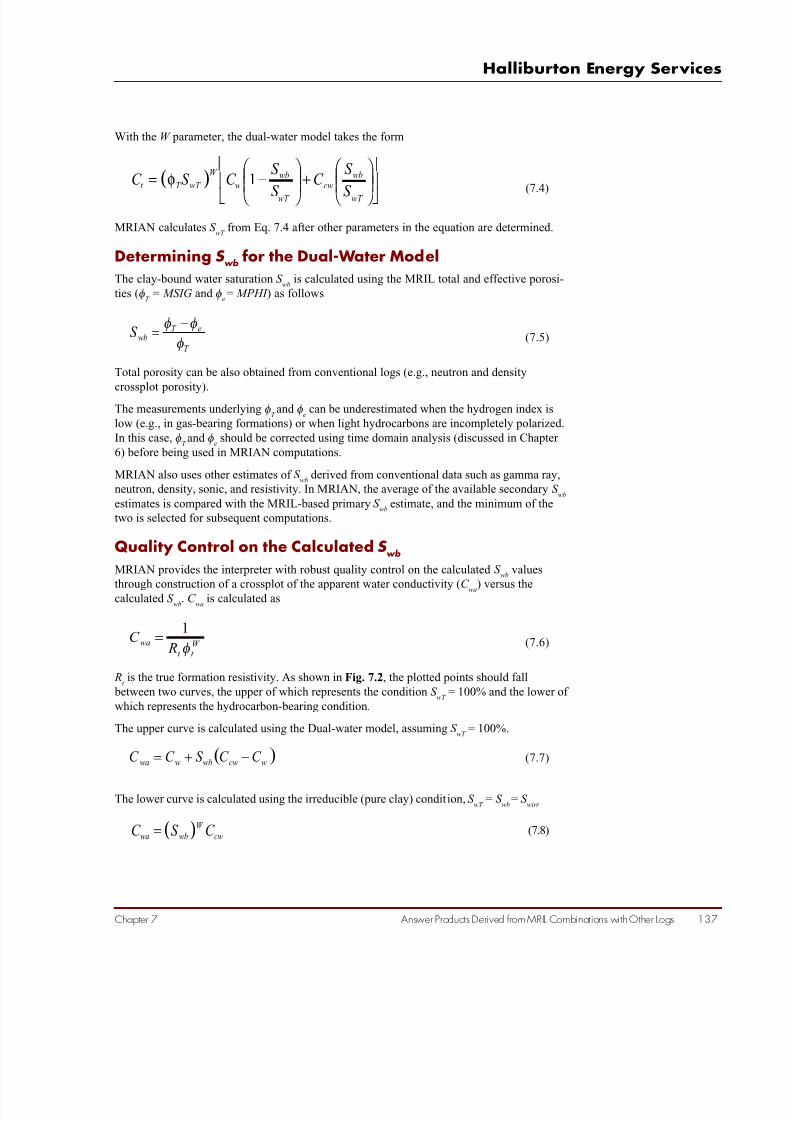
7/28/2019 NMR Logging Principles and Applications
http://slidepdf.com/reader/full/nmr-logging-principles-and-applications 155/253
Answer Products Derived from MRIL Combinations with Other Logs 137
Halliburton Energy Services
Chapter 7
With the W parameter, the dual-water model takes the form
( )
+
−=
wT
wb
cw
wT
wb
w
W
wT T t
S
S C
S
S C S C 1φ
(7.4)
MRIAN calculates S wT
from Eq. 7.4 after other parameters in the equation are determined.
Determining S wb
for the Dual-Water Model
The clay-bound water saturation S wb
is calculated using the MRIL total and effective porosi-
ties (φT
= MSIG and φe= MPHI ) as follows
T
eT
wbS
φ
φφ −= (7.5)
Total porosity can be also obtained from conventional logs (e.g., neutron and density
crossplot porosity).The measurements underlying φ
T and φ
ecan be underestimated when the hydrogen index is
low (e.g., in gas-bearing formations) or when light hydrocarbons are incompletely polarized.
In this case, φT and φ
eshould be corrected using time domain analysis (discussed in Chapter
6) before being used in MRIAN computations.
MRIAN also uses other estimates of S wb
derived from conventional data such as gamma ray,
neutron, density, sonic, and resistivity. In MRIAN, the average of the available secondary S wb
estimates is compared with the MRIL-based primary S wb
estimate, and the minimum of the
two is selected for subsequent computations.
Quality Control on the Calculated S wb
MRIAN provides the interpreter with robust quality control on the calculated S wb
values
through construction of a crossplot of the apparent water conductivity (C wa) versus thecalculated S wb
. C wa
is calculated as
W
t t
wa R
C φ
1= (7.6)
Rt is the true formation resistivity. As shown in Fig. 7.2, the plotted points should fall
between two curves, the upper of which represents the condition S wT
= 100% and the lower of
which represents the hydrocarbon-bearing condition.
The upper curve is calculated using the Dual-water model, assuming S wT
= 100%.
( )wcwwbwwa
C C S C C −+= (7.7)
The lower curve is calculated using the irreducible (pure clay) condition, S wT
= S wb
= S wirr
( )cw
W
wbwaC S C = (7.8)

7/28/2019 NMR Logging Principles and Applications
http://slidepdf.com/reader/full/nmr-logging-principles-and-applications 156/253
NMR Logging Principles and Applications
138 Answer Products Derived from MRIL Combinations with Other Logs Chapter 7
Figure 7.2— A crossplot ofC
wa vs. S
wb serves as a
quality check on thecalculated S
wb values.
Points in the plot should
generally fall between twocurves, the upper of whichrepresents points withS
wT = 100% and the lower
of which represents pointswith S
wT = S
wb .
50
45
40
35
30
25
20
15
10
0 0.1 0.2 0.3 0.4 0.5 0.6 0.7 0.8 0.9 1.0
C w a
G a m m a R a y
MRIL S wb Well: C/tp ClayZone: 15,500.000 to 16,100.000 ft
C cw
S w T = 1 0 0 %
S S
W
=, d e
p e n d s o
n
w b
w T
110
93.3333
76.6667
60
43.3333
26.6667
10
5
0
( m h o \ m )
o m 0 0 0 9 0 9
Determination of the W exponent in MRIAN
The W exponent described in Eq. 7.3 is automatically determined throughout the MRIAN
processing scheme. By solving Eq. 7.4, W can be estimated from
)log(
)/()/1(log
wT T
wT wbcwwT wbw
t
S
S S C S S C
C
W φ
+−= (7.9)
W will fall between values obtained from Eq. 7.9 at two extreme conditions:
• 100% water saturation
• Hydrocarbon bearing at irreducible condition
At 100% water saturation, the value of W is designated W w
and can be calculated from
Eq. 7.9 using S wT
= 1.0:
)log(
)(log
T
wcwwbw
t
w
C C S C
C
W φ
−+= (7.10)
At irreducible condition, the value of W is designated W i and can be calculated from Eq.7.9 using S
wT = S
wirr :
)log(
/)(log
wirr T
wirr wcwwbw
t
i
S
S C C S C
C
W φ
−+= (7.11)
7/28/2019 NMR Logging Principles and Applications
http://slidepdf.com/reader/full/nmr-logging-principles-and-applications 157/253
Answer Products Derived from MRIL Combinations with Other Logs 139
Halliburton Energy Services
Chapter 7
where
T
wbT
wirr
BVI S S
φ
φ += (7.12)
with BVI being obtained from an MRIL log.
In a normal hydrocarbon-bearing formation, W will always be less than W w
and greater
than W i.
W i< W < W
w(7.13)
MRIAN uses the following empirical relation to calculate W 4:
W = W Q
= 1.65 + 0.4( MPHI
BVI ) (7.14)
If W Q > W w, then MRIAN sets W Q = W w and recognizes the zone as being wet. If W Q < W i,then MRIAN sets W
Q= W
iand recognizes the zone as being at irreducible water saturation.
Calculation of S wT
in MRIAN
MRIAN uses the S wb
and W Q
values to calculate S wT
from the Dual-Water model as described
before. Using S wT
, MRIAN then calculates water-filled porosity (φwT
), bulk volume of water in
effective porosity (CBVWE ), and hydrocarbon pore volume (φh). These parameters take the
forms
T wT wT S φφ = (7.15)
MCBW CBVWE wT −=φ (7.16)
CBVWE eh −=φφ (7.17)
MCBW is the MRIL-derived volume of clay-bound water, and φe
is the effective porosity.
Parameters Affecting MRIAN Calculations
Rw
is generally one of the most important parameters involved in the water saturation model,
and every available source should be exploited to determine an accurate value for Rw. The
salinity of a sample of formation water can be a good source. In addition, apparent Rw
values
can be obtained from Archie transforms of Rt and porosity, as well as from BVI information.
Spontaneous potential (SP) measurements can be also used to estimate Rw.5 However, it
should be noted that SP, resistivity, and porosity measurements are affected by hydrocarbons.
MRIL Data Acquisition for MRIANThe MRIL data required for MRIAN processing can be acquired with a total-porosity
logging activation, which acquires two types of CPMG echo trains: fully polarized and
partially polarized. The fully polarized echo train is acquired by using a long TW and a TE of
0.9 or 1.2 ms. These parameter values constitute a standard-T 2
logging activation as dis-cussed before. The partially polarized echo train is acquired with a short TE (0.6 ms) and a
short TW (20 ms).

7/28/2019 NMR Logging Principles and Applications
http://slidepdf.com/reader/full/nmr-logging-principles-and-applications 158/253
NMR Logging Principles and Applications
140 Answer Products Derived from MRIL Combinations with Other Logs Chapter 7
After a long polarization time (TW ), a fully polarized echo train is acquired. Then, a partially
polarized sequence is recorded. This sequence consists of 50 echo trains with 10 echoes per
train. The first two echo trains are used to stabilize the system and are subsequently dis-
carded. The remaining trains are stacked and used for computing the part of the decay
spectrum that falls in T 2 bins with T 2 ≤ 4 ms. This part of the spectrum represents water insmall pores and clay-bound water. The working assumption is that the partially polarized
echo train represents the signal from clay-bound water. The two T 2
distributions (one from the
fully polarized echo train and one from the partially polarized echo train) when combined,
form a continuous T 2
distribution from 0.5 ms to more than 1,000 ms and provide a good
estimation of total porosity.
The principle of total-porosity logging is illustrated in Fig. 7.3
At the wellsite, total-porosity logging provides bin data, a T 2
distribution from the fully polar-
ized echo train, a T 2
distribution from the partially polarized echo train, apparent MCBW ,
MPHI , BVI , MFFI , and MPERM , as shown in Fig. 7.4. The wellsite products, such as MFFI,
BVI, and MPERM are calculated with the default T 2cutoff
and permeability parameters.
MRIL data acquired with dual-TW , dual-TE , or standard-T 2
logging activations can also be
used in MRIAN analysis. In the cases where dual-TW or dual-TE logging is used, the effec-tive porosity MPHI should be taken from the long-TW echo train in dual-TW logging and
from the short-TE echo train in dual-TE logging. Other porosity sources, such as a density/
neutron crossplot, are needed for the total porosity.
Figure 7.3 —Total-porositylogging acquires fullypolarized echo trains using
short TE (0.9 or 1.2 ms)and partially polarizedecho trains using veryshort TE (0.6 ms) andshort TW (20 ms). The T
2
distributions correspondingto these echo trains aredisplayed at the bottompart of the figure.
M 0
0
Porosity
P o la r iz a tio n
Partially PolarizedFully Polarized
Fully Polarized Partially Polarized
AcquisitionPolarization
BVI FFI +Clay-bound Water
0 1 10 100 1,000T 2 Relaxation Time (ms)
0 1 10 100 1,000T 2 Relaxation Time (ms)
o m 0 0 0 9 1 1
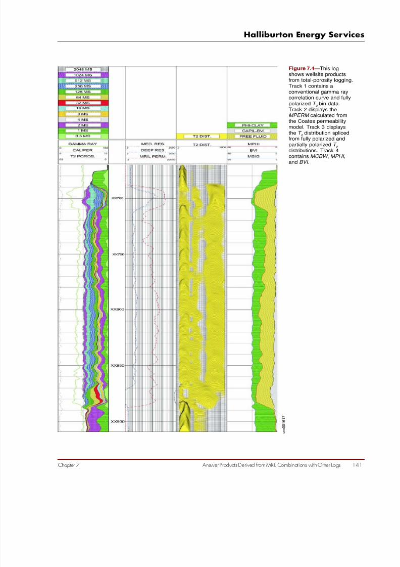
7/28/2019 NMR Logging Principles and Applications
http://slidepdf.com/reader/full/nmr-logging-principles-and-applications 159/253
Answer Products Derived from MRIL Combinations with Other Logs 141
Halliburton Energy Services
Chapter 7
Figure 7.4 —This logshows wellsite productsfrom total-porosity logging.Track 1 contains aconventional gamma ray
correlation curve and fullypolarized T 2
bin data.Track 2 displays theMPERM calculated fromthe Coates permeabilitymodel. Track 3 displaysthe T
2 distribution spliced
from fully polarized andpartially polarized T
2
distributions. Track 4contains MCBW , MPHI ,and BVI .
o m 0 0 1 6 1 7

7/28/2019 NMR Logging Principles and Applications
http://slidepdf.com/reader/full/nmr-logging-principles-and-applications 160/253
NMR Logging Principles and Applications
142 Answer Products Derived from MRIL Combinations with Other Logs Chapter 7
MRIAN Applications
Low-Resistivity Reservoir 1
Fig. 7.5 shows a MRIAN example of the same well from the Gulf of Mexico, U.S.A., that wasshown in Fig. 7.4. Track 1 contains gamma ray, caliper, and T
2bin data. Track 2 contains
resistivity data and MRIL permeability derived from the Coates model. Track 3 displays the T 2
distribution for clay-bound water and the long-TW echo trains. In the interval from XX690 to
XX870, the hydrocarbons are oil, as indicated by the signals at long T 2. Track 4 displays the
MRIAN results.
MRIL data for this example were acquired through total-porosity logging and through dual-
TW logging. Total-porosity logging was used to determine clay-bound water, capillary-bound
water, and free fluids. Dual-TW logging with TW values of 1 and 8 s was used to type the
hydrocarbons and to make porosity corrections for under-polarization and hydrogen-index
effects. Based on the MRIL BVI , FFI , and CBW , the observed reduction in resistivity from
Zone A (XX690 to XX710) to Zone B (XX710 to XX870) was attributed to the increase in
clay-bound water (Track 3) and not the presence of movable water. The MRIAN results
suggested that Zone B was at irreducible water condition (Track 4) and had sufficient permeability (Track 2) to produce the movable hydrocarbons.
Fig. 7.6 shows the results of TDA (Track 5) and TDA/MRIAN (Track 6) for the same well as
Fig. 7.4 and 7.5. In the TDA/MRIAN analysis, TDA provides a corrected effective porosity
for MRIAN inputs. For this specific well, which was drilled with oil-based mud, both TDA
and TDA/MRIAN results agree well.
Low-Resistivity Reservoir 2
Because MRIL data can provide estimates of irreducible water saturation, one of the advan-
tages that MRIL logging has brought to petrophysical interpretation is the capability of more
readily identifying low-resistivity pay zones, as seen in the previous example. If a rock
contains a large amount of bound water, then formation resistivity is low, and in an initial
analysis, the zone may appear wet. MRIL data, though, immediately shows the water to be
bound and the zone as still having potential. In the conventional data presented in Fig. 7.7,the sand below XX200 has resistivity (Track 2) about 0.5 ohm-m and average neutron-
density porosity (Track 4) about 38%. A standard first-pass analysis of S w
performed with
these values would label this zone as wet.
Fig. 7.8 shows MRIL data acquired with a standard-T 2
logging activation for the same sand.
Track 1 contains the T 2-distribution bin data, Track 2 contains formation permeability from
the Coates model, and Track 3 contains the T 2
distribution in a variable-density display. Track
4 represents the irreducible water ( BVI ; shaded gray) and the free-fluid porosity (shaded
yellow). BVI gradually increases with depth, suggesting that the sand is fining downward. (As
sand grains become finer, the volume of capillary-bound water that they hold increases.)
Also, comparison of the BVI with the resistivity profile shows that the resistivity decreases
where the bound water increases. Because the initial MRIL data were encouraging, the sand
was investigated further through MRIAN analysis. Fig. 7.9 contains the MRIAN interpreta-
tion of the combination of MRIL and resistivity data. Track 1 shows gamma ray, caliper, SP,and T
2bin data. Track 2 displays the resistivity and MRIL permeability. Track 3 contains the
variable-density presentation of the T 2
distribution. Track 4 shows MRIAN fluid analysis,
where capillary-bound water is shaded in gray, movable water in blue, and hydrocarbon in
green. The MRIAN analysis clearly shows that the zone does not contain any movable water
and will produce only oil. The interval below XX200 was tested and produced oil with
no water.

7/28/2019 NMR Logging Principles and Applications
http://slidepdf.com/reader/full/nmr-logging-principles-and-applications 161/253
Answer Products Derived from MRIL Combinations with Other Logs 143
Halliburton Energy Services
Chapter 7
Figure 7.5 —In this wellfrom the Gulf of Mexico,U.S.A. (same well asshown in Fig. 7.4),conventional Archie S
w
analysis indicated that thezone from xx710 to xx870was wet. MRIAN analysis,however, suggested thezone was at irreduciblewater condition (Track 4)and had sufficientpermeability (Track 2) toproduce the movablehydrocarbons.
o m 0 0 1 6 1 8

7/28/2019 NMR Logging Principles and Applications
http://slidepdf.com/reader/full/nmr-logging-principles-and-applications 162/253
NMR Logging Principles and Applications
144 Answer Products Derived from MRIL Combinations with Other Logs Chapter 7
Figure 7.6 —TDA andTDA/MRIAN results(Tracks 5 and 6, respec-tively) agree well in this oilwell drilled with oil-based
mud. This well is the sameas the one depicted inFigs. 7.4 and 7.5.
o m 0 0 1 6 1 9

7/28/2019 NMR Logging Principles and Applications
http://slidepdf.com/reader/full/nmr-logging-principles-and-applications 163/253
Answer Products Derived from MRIL Combinations with Other Logs 145
Halliburton Energy Services
Chapter 7
Figure 7.7 —Conventionaldata shows the lower zoneof this well (below XX200)to be water-wet because ofthe very low resistivity.
o m 0 0 1 6 2 0
Figure 7.8 —This MRIL logwas run in the same wellas the log of Fig. 7.7 andshows in Track 4 that BVI
increases with depth.
o m 0 0 1 6 2 1

7/28/2019 NMR Logging Principles and Applications
http://slidepdf.com/reader/full/nmr-logging-principles-and-applications 164/253
NMR Logging Principles and Applications
146 Answer Products Derived from MRIL Combinations with Other Logs Chapter 7
Figure 7.9 —The MRIANresults shown in Track 4of this log were obtainedfrom a combined analysisof the conventional
logging data in Fig. 7.7and the MRIL data in Fig.7.8. These results showthat the whole zone iswater-free pay, whichtesting confirmed.
o m 0 0 1 6 2 2
Gas-Influx Monitoring with MRIL in an Arabian Gulf Car-bonate
A gas-injection project was undertaken in a light-oil reservoir in the Arabian Gulf. Two
problems facing gas monitoring on this project were the effect of salinity on wireline logs and the inadequate porosity measurements made by logging-while-drilling (LWD) devices. (The
LWD porosity always underestimated the reservoir porosity by 3 to 4 p.u.)
MRIL logs were run in this reservoir because of the MRIL gas-monitoring capability through
Time Domain Analysis and because of the negligible effect of formation water salinity on
MRIL measurements. In particular, MRIL, LWD neutron, and LWD density logs were
recorded in a re-entry well with 59° deviation. The original borehole was cored, but the re-
entry borehole was not. MRIL, LWD, and core porosities were statistically compared. The
average gas-corrected MRIL porosity over the cored zone was 21 p.u., which compared very
well with the average core porosity of 20.8 p.u. The average LWD porosity over the same
zone was 17.4 p.u.
Tracks 6 and 7 of the log in Fig. 7.10 show the MRIL results for, respectively, both Time
Domain Analysis and MRIAN analysis. TDA showed four types of fluids in the flushed zone:
gas influx (shaded red), residual oil (green), movable water (blue), and irreducible water
(gray). Track 7 shows the MRIAN analysis, which indicated that the reservoir was at irreduc-
ible water saturation and no movable water was present. Combining the results of both
analyses suggests that the movable water interpreted by TDA was filtrate from the water-
based mud.

7/28/2019 NMR Logging Principles and Applications
http://slidepdf.com/reader/full/nmr-logging-principles-and-applications 165/253
Answer Products Derived from MRIL Combinations with Other Logs 147
Halliburton Energy Services
Chapter 7
The differences in the results derived from TDA and MRIAN fluid identification are due to
differences in the depths of investigation of the measurements that provided the data for the
analyses. All data used for TDA are from measurements in the near-wellbore zone, which for
water-based mud normally has a higher water saturation than the virgin zone. MRIAN uses
the deep resistivity measurement, which is dominated by the virgin zone saturation, so
MRIAN output is more representative of saturation there. When TDA is used together with
MRIAN, the flushed-zone and virgin-zone saturations can be compared. TDA provides
information for typing and quantifying fluids, and can furnish key data for MRIAN process-
ing, such as effective porosity corrected for hydrogen-index and for polarization effects. If
MRIL total-porosity measurements are available, then clay-bound water saturation and total
porosity can be also derived from MRIL data alone, and a TDA/MRIAN combination can be
run without conventional porosity data. Comparison of TDA and MRIAN answer products
reveals changes in S w between the invaded zone and the virgin zone. This change is depen-dent on mud type. Fig. 7.11 illustrates the principles of the TDA/MRIAN combination when
log data are acquired under water-based mud conditions.
Figure 7.10 —TDA andMRIAN analyses wereperformed on MRIL dataacquired in a gas-injectionwell in a light-oil reservoir
in the Arabian Gulf. Track1 contains T 2
bin data andconventional SP andgamma ray curves. Track 2shows permeability derivedfrom the standard Coatesmodel; this track alsoshows LWD resistivitydata. Track 3 displays theT
2distribution in variable
density format. Track 4contains T
2distributions of
data acquired with longTW and short TW . Track 5is the differential spectrum.Track 6 contains TDAresults. Track 7 contains
MRIAN results. Becausethis display was custom-ized for the client, it differsfrom most other displays inthis book.
o m 0 0 1 6 2 3
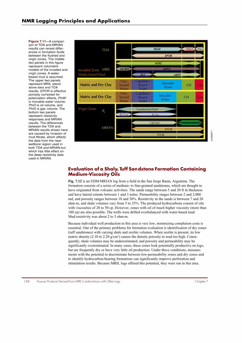
7/28/2019 NMR Logging Principles and Applications
http://slidepdf.com/reader/full/nmr-logging-principles-and-applications 166/253
NMR Logging Principles and Applications
148 Answer Products Derived from MRIL Combinations with Other Logs Chapter 7
Figure 7.11 —A compari-son of TDA and MRIANresults can reveal differ-ences in formation fluidsbetween the flushed and
virgin zones. The middletwo panels in this figurerepresent volumetricmodels of the invaded andvirgin zones. A water-based mud is assumed.The upper two panelsrepresent MRIL stand-alone data and TDAresults. EPOR is effectiveporosity corrected forpolarization effects, PhiW
is movable water volume,PhiO is oil volume, andPhiG is gas volume. Thebottom two panelsrepresent resistivity
responses and MRIANresults. The differencesbetween the TDA andMRIAN results shown hereare caused by invasion ofmud filtrate, which affectsthe data from the near-wellbore region used inboth TDA and MRIAN butwhich has little effect onthe deep-resistivity dataused in MRIAN.
o m 0 0 0 9 1 7
TDA
R t Virgin Zone
Invaded ZoneWater-based Mud
MRIL
MRIAN
PhiW
MSIG
MPHI MCBW
MFFI BVI
PhiO PhiG
EPOR
Matrix and Dry ClayClay-boundWater
Capillary-boundWater
MovableWater
Oil Gas
Matrix and Dry ClayClay-boundWater
Capillary-boundWater
MovableWater
Oil Gas
@ Cw
CBVWE
EPOR
TPOR
@ Ccw
PhiW
MPHI
MFFI BVI
EPOR
MSIG
MCBW
Conductive Fluid
Hydrocarbon
Evaluation of a Shaly, Tuff Sandstone Formation ContainingMedium-Viscosity Oils
Fig. 7.12 is an EDM/MRIAN log from a field in the San Jorge Basin, Argentina. Theformation consists of a series of medium- to fine-grained sandstones, which are thought to
have originated from volcanic activities. The sands range between 5 and 20 ft in thickness
and have lateral extents between 1 and 3 miles. Permeability ranges between 2 and 2,000
md, and porosity ranges between 10 and 30%. Resistivity in the sands is between 7 and 20
ohm-m, and shale volumes vary from 5 to 25%. The produced hydrocarbons consist of oils
with viscosities of 20 to 50 cp. However, zones with oil of much higher viscosity (more than
100 cp) are also possible. The wells were drilled overbalanced with water-based mud.
Mud resistivity was about 2 to 3 ohm-m.
Because individual well production in this area is very low, minimizing completion costs is
essential. One of the primary problems for formation evaluation is identification of dry zones
(tuff sandstones) with varying shale and zeolite volumes. When zeolite is present, its low
matrix density (2.10 to 2.20 g/cm3) causes the density porosity to read too high. Conse-
quently, shale volumes may be underestimated, and porosity and permeability may besignificantly overestimated. In many cases, these zones look potentially productive on logs,
but are frequently dry or have very little oil production. Under these conditions, measure-
ments with the potential to discriminate between low-permeability zones and dry zones and
to identify hydrocarbon-bearing formations can significantly improve perforation and
stimulation results. Because MRIL logs offered this potential, they were run in this area.

7/28/2019 NMR Logging Principles and Applications
http://slidepdf.com/reader/full/nmr-logging-principles-and-applications 167/253
Answer Products Derived from MRIL Combinations with Other Logs 149
Halliburton Energy Services
Chapter 7
Figure 7.12 —This logincludes results of EDM/ MRIAN processing. Track 1contains conventionalcorrelation log curves
(gamma ray, SP, caliper)and T 2
bin data. Track 2contains resistivity dataand MRIL-derived perme-ability. The waveforms inTrack 3 represent the T
2
distribution derived fromthe partially polarized echotrains used for determiningclay-bound water and fromthe fully polarized echotrains acquired with shortTE . The differential spectrain Track 4 are the differ-ence between two T
2
distributions from echotrains acquired with TE =
3.6 ms and TW = 300 and3,000 ms. The vertical linein Track 4 represents amaximum value for thewater signal (T
2DW = 44
ms). Sharp changes in theT
2spectra are evident at
the oil/water contact.Track 5 contains the resultsof MRIAN analysis for fluidcomposition and volume(clay-bound water, hydro-carbon, free water, andcapillary-bound water).
o m 0 0 1 6 2 4
An MRIL total-porosity activation (TE = 0.6 and 1.2 ms, and TW = 3 s) was used to establish
petrophysical properties such as clay-bound water, capillary-bound water, movable fluids,effective porosity, and permeability. A dual-TW activation (TE = 3.6 ms, and TW = 0.3 and 3
s) was used to supply measurements that would support the MRIL EDM technique for typing
and quantifying the medium-viscosity oils in the reservoir. The zones of interest in this field
often have porosity components of 256 and 512 ms in the standard T 2
distribution acquired
with TE = 1.2 ms. These components imply the presence of large, water-filled pores.
Utilizing the diffusion contrast between water and medium-viscosity oil, an upper T 2
limit of

7/28/2019 NMR Logging Principles and Applications
http://slidepdf.com/reader/full/nmr-logging-principles-and-applications 168/253
NMR Logging Principles and Applications
150 Answer Products Derived from MRIL Combinations with Other Logs Chapter 7
water (T 2 DW
) was established to be 44 ms. Therefore, any signal with T 2
value greater than 44
ms could be attributed to oil, which has an average T 2
of approximately 90 ms. Based on this
qualification, the MRIL data identified one zone from X036.5 to X042.5 that unambigu-
ously contained oil. The standard T 2
distribution shown in Track 3 was unable to distinguish
the oil/water contact in this zone. The EDM method shown in Track 4, however, clearlyidentified the contact. The operator completed this zone without stimulation and produced
554 B/D of fluid with a trace of water.
Utilizing the Coates equation with a customized C = 6.0, the MRIL tool provides a continu-
ous permeability curve. The operator has observed that zones with permeability values less
than 1 md are poor producers. By utilizing the MRIL permeability, fracture stimulation
performance is significantly improved in this reservoir. The MRIL log was found to give a
representative value of reservoir permeability within the drainage area of the well, and this
permeability allowed a reasonable estimation of the after-fracture production. Zones with kh
value (where k is zone permeability, and h is zone thickness) above 2 md/m and pressure at
least 80% of the original reservoir pressure were targeted for treatment. However, the
production in some zones above 2 md/m did not increase after fracturing, which suggested
the possible influence of zeolite. These zones can easily be identified by comparing the
MRIL-derived porosity to porosity derived from the neutron-density crossplot. Zones inwhich the MRIL effective porosity is substantially less than neutron-density porosity can be
identified as tuff sands that will be non-productive.
As a result of the integration of MRIL into the logging program, the number of non-commer-
cial completed zones decreased, and costs associated with production tests and stimulation
were significantly reduced. The EDM results for the other two zones that appeared promis-
ing on the log of Fig. 7.12 have been also confirmed by production results.
MRIAN in a Light-Hydrocarbon Well
Fig. 7.13 shows MRIAN results from a well logged with dual-TE activation. (The dual-TE
log was shown in Fig. 6.13.) Track 1 includes conventional gamma ray and caliper curves
along with T 2
bin data. Track 2 shows resistivity data and MRIL-derived permeability. Track
3 displays the T 2
distributions from the short-TE echo trains. Track 4 includes neutron and
density porosities and MRIAN answer products: volumes of capillary-bound water, free
water, and hydrocarbons. The MRIAN results, resistivity data, and T 2
distributions clearly
indicate a water/hydrocarbon contact at approximately X050 ft. Comparison of the MRIL
porosity with the neutron and density porosities suggests that the hydrogen index of the zone
above X050 ft is less than 1. The T 2
distribution in Track 3 shows that the peak values for the
hydrocarbon T 2
are around 256 ms between X000 and X050 ft, thus this interval should not
contain gas. Above X000 ft, however, the amplitudes of the T 2
peak at 256 ms are significantly
reduced, and more signals appear at T2
values of approximately 40 ms, which suggests the
presence of gas. The permeability in Track 2 as it is derived from MRIL porosity is under-
estimated above X050 ft. Dual-TW data would allow a more accurate analysis of this reservoir.
Well Completion with MRIL: StiMRILStiMRIL is an interpretation program that combines the MRIL reservoir-characterizationdata (especially permeability, effective porosity, and total porosity) with other petrophysicalmeasurements to optimize the design of stimulation treatments. Compared with previouslyavailable sources of information, this combination provides easier-to-obtain and more
reliable answers to the following critical questions:
• Where are hydrocarbons located?

7/28/2019 NMR Logging Principles and Applications
http://slidepdf.com/reader/full/nmr-logging-principles-and-applications 169/253
Answer Products Derived from MRIL Combinations with Other Logs 151
Halliburton Energy Services
Chapter 7
Figure 7.13 —TheseMRIAN results werederived from dual-TE datagathered in a light-hydrocarbon reservoir. The
porosity data above X,000ft indicates gas, as doesthe T
2data. However,
between X,050 and X,000ft, the porosity data stillsuggest gas, but the T
2
data give no indication ofgas. Had dual-TW databeen acquired, it couldhave been used to resolvethis discrepancy.
o m 0 0 1 6 2 5
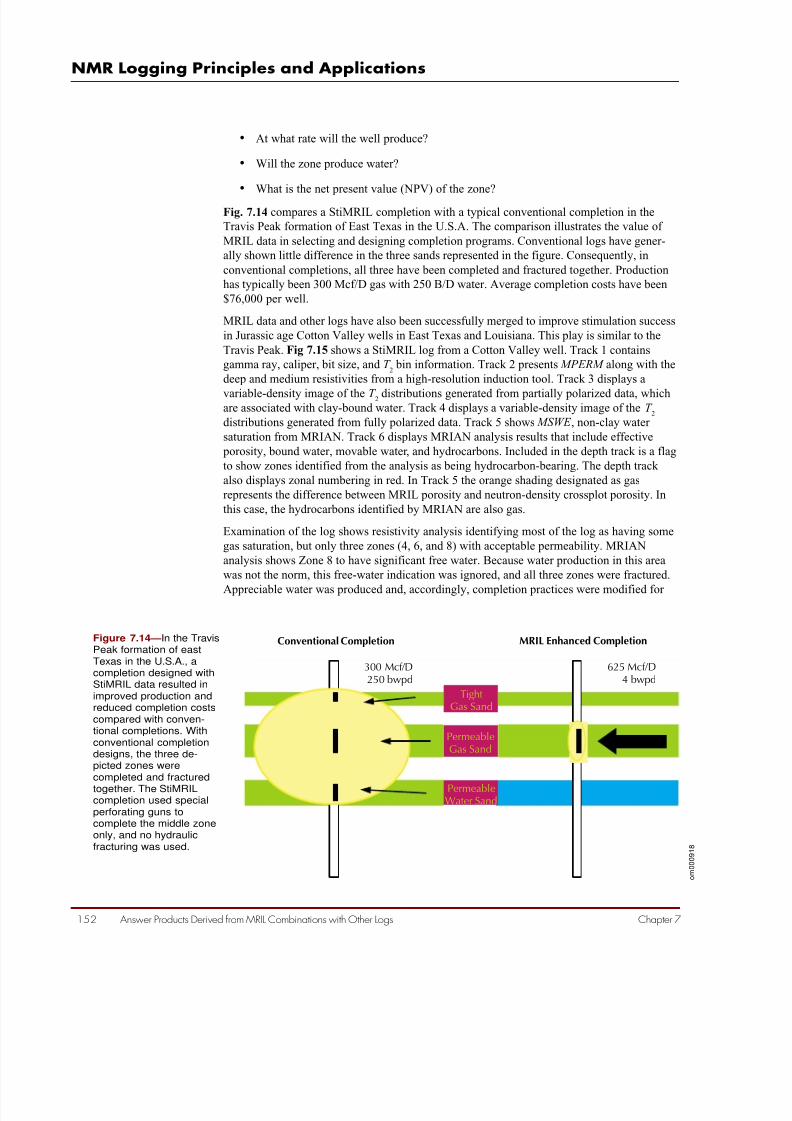
7/28/2019 NMR Logging Principles and Applications
http://slidepdf.com/reader/full/nmr-logging-principles-and-applications 170/253
NMR Logging Principles and Applications
152 Answer Products Derived from MRIL Combinations with Other Logs Chapter 7
Figure 7.14 —In the TravisPeak formation of eastTexas in the U.S.A., acompletion designed withStiMRIL data resulted inimproved production andreduced completion costscompared with conven-tional completions. Withconventional completiondesigns, the three de-picted zones werecompleted and fractured
together. The StiMRILcompletion used specialperforating guns tocomplete the middle zoneonly, and no hydraulicfracturing was used.
Conventional Completion MRIL Enhanced Completion
300 Mcf/D250 bwpd
625 Mcf/D4 bwpd
PermeableGas Sand
TightGas Sand
PermeableWater Sand
o m 0 0 0 9 1 8
• At what rate will the well produce?
• Will the zone produce water?
• What is the net present value (NPV) of the zone?
Fig. 7.14 compares a StiMRIL completion with a typical conventional completion in the
Travis Peak formation of East Texas in the U.S.A. The comparison illustrates the value of
MRIL data in selecting and designing completion programs. Conventional logs have gener-
ally shown little difference in the three sands represented in the figure. Consequently, in
conventional completions, all three have been completed and fractured together. Production
has typically been 300 Mcf/D gas with 250 B/D water. Average completion costs have been
$76,000 per well.
MRIL data and other logs have also been successfully merged to improve stimulation success
in Jurassic age Cotton Valley wells in East Texas and Louisiana. This play is similar to the
Travis Peak. Fig 7.15 shows a StiMRIL log from a Cotton Valley well. Track 1 contains
gamma ray, caliper, bit size, and T 2
bin information. Track 2 presents MPERM along with the
deep and medium resistivities from a high-resolution induction tool. Track 3 displays a
variable-density image of the T 2 distributions generated from partially polarized data, whichare associated with clay-bound water. Track 4 displays a variable-density image of the T
2
distributions generated from fully polarized data. Track 5 shows MSWE , non-clay water
saturation from MRIAN. Track 6 displays MRIAN analysis results that include effective
porosity, bound water, movable water, and hydrocarbons. Included in the depth track is a flag
to show zones identified from the analysis as being hydrocarbon-bearing. The depth track
also displays zonal numbering in red. In Track 5 the orange shading designated as gas
represents the difference between MRIL porosity and neutron-density crossplot porosity. In
this case, the hydrocarbons identified by MRIAN are also gas.
Examination of the log shows resistivity analysis identifying most of the log as having some
gas saturation, but only three zones (4, 6, and 8) with acceptable permeability. MRIAN
analysis shows Zone 8 to have significant free water. Because water production in this area
was not the norm, this free-water indication was ignored, and all three zones were fractured.
Appreciable water was produced and, accordingly, completion practices were modified for

7/28/2019 NMR Logging Principles and Applications
http://slidepdf.com/reader/full/nmr-logging-principles-and-applications 171/253
Answer Products Derived from MRIL Combinations with Other Logs 153
Halliburton Energy Services
Chapter 7
Figure 7.15 —This StiMRILstandard log presentationcontains MRIL data andthe results of MRIANanalysis. Zones deter-
mined with StiMRIL aredelineated by the red linesextending across all tracksand are numbered in thefar-left track. The far-lefttrack also contains blackpay flags that resultedfrom StiMRIL analysis.
o m 0 0 1 6 2 6
7/28/2019 NMR Logging Principles and Applications
http://slidepdf.com/reader/full/nmr-logging-principles-and-applications 172/253
NMR Logging Principles and Applications
154 Answer Products Derived from MRIL Combinations with Other Logs Chapter 7
subsequent wells. In particular, only Zone 4 is being fractured. Zone 6 is not fractured
because fractures there might extend through the thin seal separating Zone 6 and Zone 8
which contains free water. Furthermore, as estimated from permeability and thickness, Zone
6 would only flow at 17% of the rate of Zone 4.
References
1. Coates, G.R., Gardner, J.S., and Miller, D.L., 1994, Applying pulse-echo NMR to shaly
sand formation evaluation, paper B, 35th Annual SPWLA Logging Symposium Transac-
tions, 22 p.
2. Clavier, C., Coates, G., and Dumanoir, J., 1977, The theoretical and experimental bases
for the dual water model for interpretation of shaly sands, SPE 6859, 16 p.
3. Ostroff, G.M., Shorey, D.S., and Georgi, D.T., 1999, Integration of NMR and conven-
tional log data for improved petrophysical evaluation of shaly sands, 40th Annual
SPWLA Logging Symposium Transactions, 14 p.
4. Coates, G.R., and Howard, A.D., 1992, Core data and the MRIL show a new approach toformation factor, SCA-9207, in 6th annual technical conference preprints (33rd Annual
SPWLA Logging Symposium Transactions, v. 3): Society of Core Analysts, Society of
Professional Well Log Analysts Chapter-at-Large, 14 p.
5. Coates, G., and Miller, D., 1997, Confirming Rw by reconstructing the SP using forma-
tion evaluation results employing gradient field magnetic resonance logs, paper VV, 38th
Annual SPWLA Logging Symposium Transactions, 12 p.
More NMR logging application case studies can be found in following literature:
Altunbay, M., Edwards, C.M., and Georgi, D.T., 1997, Reducing uncertainty in reservoir
description with NMR-log data, SPE 38027, 1997 SPE Asia Pacific Oil and Gas Confer-
ence Proceedings, p. 99–108.
Altunbay, M., Georgi, D., and Takezaki, H., 1997, Improving S wir and permeability estimates
in carbonates with hydraulic units and NMR-variable T 2-partitioning coefficients, paper I,
3rd SPWLA Well Logging Symposium of Japan Proceedings, 9 p.
Austin, J.M., and Faulkner, T.L., 1993, Magnetic resonance imaging log evaluates low-
resistivity pay, American Oil and Gas Reporter , v. 36, no. 8, p. 52–57.
Castelijns, C., Badry, R., Decoster, E., Hyde, C., 1999, Combining NMR and formation
tester data for optimum hydrocarbon typing, permeability and producibility estimation,
40th Annual SPWLA Logging Symposium Transactions Annual Logging Symposium, 14 p.
Chang, D., et al., 1994, Effective porosity, producible fluid and permeability in carbonates
from NMR logging, paper A, 35th Annual SPWLA Logging Symposium Transactions,
21 p. Later published in 1997 in The Log Analyst , v. 38, no. 2, p. 60–72.
Coates, G.R., et al., 1993, Restrictive diffusion from uniform gradient NMR well logging,SPE 26472, 1993 SPE Annual Technical Conference and Exhibition Proceedings, v.Ω
(Formation evaluation and reservoir geology), p. 575–590.
Coope, D.F., 1994, Petrophysical applications of NMR in the North Sea, paper Z, 16th
SPWLA European Formation Evaluation Symposium Transactions, 12 p. Also published
7/28/2019 NMR Logging Principles and Applications
http://slidepdf.com/reader/full/nmr-logging-principles-and-applications 173/253
Answer Products Derived from MRIL Combinations with Other Logs 155
Halliburton Energy Services
Chapter 7
in 1994 as Petrophysical applications of NMR, Dialog (London Petrophysical Society
Quarterly Newsletter), v. 2, no. 4, October, p. 8–10.
Corbelleri, A., et al., 1996, Application of the magnetic resonance logging in San Jorge basin
(Argentina), paper VV, 37th Annual SPWLA Logging Symposium Transactions, 12 p.
Crary, S., Pellegrin, F., and Simon, B., 1997, NMR applications in the Gulf of Mexico, paper
PP, 38th Annual SPWLA Logging Symposium Transactions, 13 p.
Crowe, B., et al., 1997, Measuring residual oil saturation in west Texas using NMR, paper JJ,
38th Annual SPWLA Logging Symposium Transactions, 12 p.
Cunningham, A.B., and Jay, K.L., 1991, Field experience using the nuclear magnetic logging
tool for quantifying microporosity and irreducible water saturation, paper EE, 32nd
Annual SPWLA Logging Symposium Transactions, 23 p.
Dodge, W.S., Shafer, J.L., and Guzman-Garcia, A.G., 1995, Core and log NMR measure-
ments of an iron-rich glauconitic sandstone reservoir, paper O, 36th Annual SPWLA
Logging Symposium Transactions, 12 p.
Dodge, W. S., et al., 1998, A case study demonstrating how NMR logging reduces comple-
tion uncertainties in low porosity, tight gas sand reservoirs, 39th Annual SPWLA Logging
Symposium Transactions, 14 p.
Egbogah, E.O., and Amar, Z.H.B.T., 1997, Accurate initial/residual saturation determination
reduces uncertainty in further development and reservoir management of the Duland
field, offshore peninsular Malaysia, SPE 38024, 1997 SPE Asia Pacific Oil and Gas
Conference Proceedings, p. 79–90.
Eidesmo, T., Relling, O., and Rueslatten, H., 1996, NMR logging of mixed-wet North Sea
sandstone reservoirs, paper PP, 37th Annual SPWLA Logging Symposium Transactions,
14 p.
Flaum, C., Kleinberg, R.L., and Bedford, J., 1998, Bound water volume, permeability, and
residual oil saturation from incomplete magnetic resonance logging data, UU, 39th
Annual SPWLA Logging Symposium Transactions, 11 p.
Flolo, L.H., 1998, Getting the hydrocarbon volume right—a quantitative use of NMR data in
water saturation modeling, 39th Annual SPWLA Logging Symposium Transactions.
Freeman, R., et al., 1998, Combining NMR and density logs for petrophysical analysis in
gas-bearing formations, 39th Annual SPWLA Logging Symposium Transactions.
Gibson, B-D., et al., 1995, Nuclear magnetic resonance applications in North America,
paper H, 1st Annual SPWLA Well Logging Symposium of Japan Proceedings, 14 p.
Gossenberg, et al., 1996, A new petrophysical interpretation model for clastic rocks based on
NMR, epithermal neutron and electromagnetic logs, paper M, 37th Annual SPWLA
Logging Symposium Transaction, 13 p.
Gumilar, B., et al., 1996, Signal processing method for multiexponentially decaying signals
and an analysis of low-contrast pay in Telisa sands packages in central Sumatra, paper IPA96-2-2-123, 25th Annual Indonesian Petroleum Association Convention Proceedings,
v. 2, p. 175–187.
Guest, R., et al., 1998, Case studies of nuclear magnetic resonance in Texas and Louisiana
Gulf Coast area, 39th Annual SPWLA Logging Symposium Transactions.
7/28/2019 NMR Logging Principles and Applications
http://slidepdf.com/reader/full/nmr-logging-principles-and-applications 174/253
NMR Logging Principles and Applications
156 Answer Products Derived from MRIL Combinations with Other Logs Chapter 7
Hassoun, T.H., Zainalebedin, K., and Minh, C.C., 1997, Hydrocarbon detection in low-
contrast resistivity pay zones, capillary pressure and ROS determination with NMR
logging in Saudi Arabia, SPE 37770, 10th SPE Middle East Oil Show Conference
Proceedings, v. 2, p. 127–143.
Hodgkins, M.A., and Howard, J.J., 1999, Application of NMR logging to reservoir character-
ization of low resistivity sands in the Gulf of Mexico, AAPG Bulletin , v. 83, no. 1,
p.114–127.
Hook, J., Basan, P., and Lowden, B., 1996, The MRIL log in a low porosity and permeability
formation, paper N, 37th Annual SPWLA Logging Symposium Transactions, 13 p.
Horkowitz, J.P., et al., 1995, Residual oil saturation measurements in carbonates with pulsed
NMR logs, paper Q, 36th Annual SPWLA Logging Symposium Transactions, 12 p. Later
published in 1997 in The Log Analyst , v. 38, no. 2, p. 73–83.
Howard, A., 1996, MRI logging tools locate water-free production, American Oil and Gas
Reporter , v. 39, no. 11, October, p. 70, 72–74.
Howard, J., Williams, J., and Thorpe, D., 1997, Permeability from nuclear magnetic reso-
nance logging in a gas-condensate field, paper XX, 38th Annual SPWLA Logging Symposium Transactions, 13 p.
Hussein, S.M., et al., 1999, Using NMR and electrical logs for enhanced evaluation of
producibility and hydrocarbon reserves in gas reservoirs with high irreducible water
saturation, 40th Annual SPWLA Logging Symposium Transactions, 9 p.
Latif, A.A., et al., 1997, Borehole nuclear magnetic resonance—experience and reservoir ap-
plications in west Kuwait carbonate reservoirs, SPE 37771, 10th SPE Middle East Oil
Show Conference Proceedings, v. 2, p. 145–154.
Logan, W.D., et al., 1997, Practical application of NMR logging in carbonate reservoirs,
SPE 38740, 1997 SPE Annual Technical Conference and Exhibition Proceedings, v.Ω
(Formation evaluation and reservoir geology), p. 203–215.
Lomax, J., and Howard, A., 1994, New logging tool identifies permeability in shaly sands,
Oil and Gas Journal , v. 92, no. 51, December 19, p. 104–108.
Looyestijn, W., 1996, Determination of oil saturation from diffusion NMR logs, paper SS,
37th Annual SPWLA Logging Symposium Transactions, 14 p.
Looyestijn, W., Schiet, M., and Runia, J., 1994, Successful field test of nuclear magnetic
resonance (NMR) logging in the Rotterdam field, paper X, 16th SPWLA European
Formation Evaluation Symposium Transactions, 11 p.
Mardon, D., et al., 1996, Characterization of light hydrocarbon-bearing reservoirs by
gradient NMR well logging—a Gulf of Mexico case study, SPE 36520, 1996 SPE Annual
Technical Conference and Exhibition Proceedings, v.Ω (Formation evaluation and
reservoir geology), p. 295–304. Also published in 1996 in condensed form in Journal of
Petroleum technology, v. 48, no. 11, p. 1035–1036.
Mirotchnik, K., Allsopp, K., and Kantzas, A., 1997, Combination of NMR and ultracentri-fuge techniques for effective carbonate reservoir characterization, paper SCA-9703, in
1997 international symposium proceedings: Society of Professional Well Log Analysts,
Society of Core Analysts Chapter-at-Large, 10 p.
7/28/2019 NMR Logging Principles and Applications
http://slidepdf.com/reader/full/nmr-logging-principles-and-applications 175/253
Answer Products Derived from MRIL Combinations with Other Logs 157
Halliburton Energy Services
Chapter 7
Nascimento, J.D.S., and Denicol, P.S., 1999, Anomalous NMR responses in highly perme-
able sandstone reservoirs: a case study, 40th Annual SPWLA Logging Symposium
Transactions.
Olesen, J.-R., et al., 1997, Evaluation of viscous oil-bearing, water flooded reservoirs, paper
T, 3rd SPWLA Well Logging Symposium of Japan Proceedings, 14 p.
Oraby, M., et al., 1997, A new NMR interpretation technique using error minimization with
variable T2 cutoff, SPE 38734, 1997 SPE Annual Technical Conference and Exhibition
Proceedings, v.Ω (Formation evaluation and reservoir geology), p. 175–181.
Oraby, M.E., and Eubanks, D.L., 1997, Determination of irreducible water saturation using
magnetic resonance imaging logs (MRIL)—a case study from east Texas, USA,
SPE 37772, 10th SPE Middle East Oil Show Proceedings, v. 2, p. 155–162.
Petricola, M.J.C., and Takezaki, H., 1996, Nuclear magnetic resonance logging—can it
minimize well testing?, SPE 36328, 7th SPE Abu Dhabi International Petroleum
Conference Proceedings, p. 740–748.
Petricola, M.J.C., and Troussaut, X., 1999, Applications of fast NMR logging in shaly gas-
bearing sands invaded by oil filtrate, 40th Annual SPWLA Logging Symposium, 10 p.
Phen, H.A., Ajufo, A., and Curby, F.M., 1995, A hydraulic (flow) unit based model for the
determination of petrophysical properties from NMR relaxation measurements, paper
SCA-9514, in International SCA symposium proceedings: Society of Professional Well
Log Analysts, Society of Core Analysts Chapter-at-Large, 12 p.
Prieto, M., et al., 1997, Conciliation of core data and log derived permeability from nuclear
magnetic resonance and Stoneley wave in northern Monagas area, eastern Venezuela,
paper WW, 38th Annual SPWLA Logging Symposium Transactions, 14 p.
Rueslatten, et al., 1998, NMR studies of an iron-rich sandstone oil reservoir, Society of Core
Analysts-9821, 10 p.
Salvignol-Bellando, A., Volokitin, Y., Slijkerman, W., Bonnie, R., 1999, The use of NMR
logging for gas reservoir characterization in a north sea play with complex and variable
rock properties, 40th Annual SPWLA Logging Symposium Transactions.
Singer, J., et al., 1997, Fast NMR logging for bound fluid and permeability, paper YY, 38th
Annual SPWLA Logging Symposium Transactions, 13 p.
Slot-Petersen, C., et al., 1998, NMR formation evaluation applications in a complex low-
resistivity hydrocarbon reservoir, paper TT, 39th Annual SPWLA Logging Symposium
Transactions.
Sutiyono, S., 1995, Magnetic resonance image log use in evaluation of low resistivity pay in
the Attaka field, paper IPA95-2.2-056, in 24th Annual Indonesian Petroleum Association
Convention Proceedings, v. 2, Jakarta, 13 p.
Tariq, S.M., Denoo, S., and Cordes, M., 1997, Permeability estimation from modern NMR
logging measurements; experiences and applications in the Rocky Mountain area,
SPE 38378, 1997 SPE Rocky Mountain Regional Meeting/Geological Association Field Conference Proceedings.
Vinegar, H., 1995, NMR log interpretation with examples, chapter 8, in Georgi, D.T., ed.,
Nuclear magnetic resonance logging short course notes, 36th annual SPWLA logging
symposium, variously paginated.

7/28/2019 NMR Logging Principles and Applications
http://slidepdf.com/reader/full/nmr-logging-principles-and-applications 176/253
NMR Logging Principles and Applications
158 Answer Products Derived from MRIL Combinations with Other Logs Chapter 7
Walsgrove, T., et al., 1997, Integration of nuclear magnetic core analysis and nuclear
magnetic resonance logs—an example from the North Sea, paper UU, 38th Annual
SPWLA Logging Symposium Transactions, 12 p. A similar paper also published in 1997
as Basan, P. Lowden, B., and Stromberg, S., Developing strategies using core analysis for
calibrating the NMR log, DiaLog (London Petrophysical Society Newsletter), v. 5, no. 6, p. 4–6.
Warrilow, I.M., et al., 1997, Nuclear magnetic resonance—a useful complement to reservoir
characterization of Brunei deltaic sequences, SPE 38025, 1997 SPE Asia Pacific Oil and
Gas Conference Proceedings, p. 91–98.
White, J., and Bedford, J., 1997, Nuclear magnetic resonance applications in the North Sea,
DiaLog (London Petrophysical Society Newsletter), v. 5, no. 6, p. 6–8.
White, J., 1997, Application of downhole magnetic resonance imaging in the North Sea,
SPE 38551, 12 p.
Widjanarko, W., 1996, Integrating nuclear magnetic resonance logging data with traditional
down hole petrophysical data to optimize new development wells strategies in the Bravo
field offshore north west Java, paper IPA96-2-2-162, 25th Annual Indonesian Petroleum
Association Convention Proceedings, v. 2, p. 205–213.
Xiao, L.Z., 1998, NMR Imaging Logging Principles and Applications (in Chinese), Science
Press, Beijing, 328 p.

7/28/2019 NMR Logging Principles and Applications
http://slidepdf.com/reader/full/nmr-logging-principles-and-applications 177/253
MRIL Job Planning 15
Halliburton Energy Service
Chapter 8
MRIL JobPlanning
Chapter 8
Previous chapters have shown that, in most reservoirs, NMR loggingdata offer an improved method, which can be used independently or incombination with conventional logging data, to determine reservoir
properties. In some complex environments (e.g. mixed-lithologyreservoirs, low-resistivity/low-contrast pay zones, low-porosity/low-
permeability formations, medium-to-heavy oil reservoirs), whereconventional logging tools may fail to unveil important reservoir
properties, NMR may be the only technique available to assess them.Reliable and accurate NMR measurements of these reservoir propertiesrequire careful, early job planning. Such planning is critical for thesuccess of the logging run. Specific formation and fluid properties can
be utilized to design an acquisition scheme that provides access to yetunknown reservoir characteristics and that optimizes the acquisition
process and thus improves the answers derived from the data. If acquisition parameters are not selected properly, answer products may
provide properties that differ significantly from the actual reservoir properties, as is demonstrated in Fig. 8.1.
The figure shows incremental and cumulative porosity and T 2
spectrafrom two sets of NMR measurements on the same core-plug. The red
curves are results derived from data acquired with insufficient echoes( NE ), insufficient polarization time (TW ), overly long echo spacing(TE ), and poor signal-to-noise ratio (S/N ). In this case, the T
2distribu-
tion is fairly broad, unimodal, and centered around 30 ms, and thecumulative porosity does not exceed 8 p.u. The blue curves are resultsobtained from data acquired with increased NE , increased TW , short-ened TE , and increased echo-train stacking to improve S/N . In thiscase, the T
2distribution is bimodal with peaks at 7 and 100 ms, and the
cumulative porosity exceeds 18 p.u.
MRIL job planning can be executed in three basic steps:
1. Determine NMR fluid properties (T 1, bulk
, T 2, bulk
, D0, and HI ).
2. Assess expected NMR responses (decay spectrum, polarization,apparent porosity) over the intervals to be logged.
3. Select activation sets and determine appropriate activation parameters (TW , TE , NE ).
All aspects of job planning involved in these steps have already beenimplicitly covered in previous chapters, but will be summarized in thischapter and demonstrated by examples. The first example continuesover several main sections of the chapter.

7/28/2019 NMR Logging Principles and Applications
http://slidepdf.com/reader/full/nmr-logging-principles-and-applications 178/253
NMR Logging Principles and Applications
160 MRIL Job Planning Chapter 8
Bulk Relaxation Time
T 1,B
, T 2,B
(s)
Water
Oil
Gas
»3
»2.1
»2.5 x 10⁴
T
298 h
T
298 h
T 1.17
r
»1.3
»1.3
»8.5 x 10⁻²
T
298 h
T
298 h
T 0.9
r
»1
»1
2.25 r
Diffusion Coefficient
D 0(10-5
cm2 /s)
Hydrogen Index
HI
Determining NMR Properties of Reservoir Fluids
The fluid properties that play a prominent role in NMR logging are
• bulk longitudinal relaxation time (T 1,B
)
• unrestricted diffusion, characterized by the coefficient ( D0)
• hydrogen index ( HI )
Values of these properties can be obtained from laboratory measurements at simulated in-situ
conditions, from measurements made at ambient conditions and extrapolated to reservoir conditions, or from global correlations (available as charts or empirical equations).1–9 The bulk longitudinal relaxation time, diffusion coefficient, and hydrogen index can be parameter-ized through the empirical equations listed in Table 8.1.
Figure 8.1 —Depending ondata-acquisition param-eters, T
2spectra can vary
significantly. Here, the redcurves represent results
obtained from dataacquired with inadequateacquisition parameters.The blue curves werederived from data acquiredwith optimized acquisitionparameters.
0.0
0.5
1.0
1.5
2.0
2.5
1
T 2 Relation Time (ms)
5
10
15
20
I n c r e m e n t a l P o r o s i t y ( p
. u . )
0.1 10 100 1,000 10,0000
C u m u l a t i v e P o r o s i t y ( p . u . )
o m
0 0 0 9 3 0
Table 8.1 —NMR Fluid Properties

7/28/2019 NMR Logging Principles and Applications
http://slidepdf.com/reader/full/nmr-logging-principles-and-applications 179/253
MRIL Job Planning 16
Halliburton Energy Service
Chapter 8
In these equations, T is the reservoir temperature in degrees Kelvin, η is the viscosity atreservoir conditions in cp, and ρ is the in-situ gas density in g/cm3. The gas density can bederived directly from PVT data measured in the well, can be calculated after solving theequation of state,10 or can be read directly from the chart in Fig. 8.2.1 The oil viscosity can be
measured, obtained from other work in the area, or roughly estimated from tables and other information about the oil.11
Figure 8.2 —Each bluecurve relates the density ρ
of natural gas (C1.1
H4.2
) tothe pressure of the gas ata specific temperature.Temperature increasesfrom the top curve to thebottom curve in 50°F
increments from 100 to350°F. The arrows indicate ρ = 0.23 g/cm3 at 8,700 psiand 300°F.
0.05
0.10
0.15
0.20
0.25
0.30
0.35
2 3 4 5 6 7 8 9 10
350°F
100°F
P (103 psia)
( r / c m 3 )
o m
0 0 0 9 3 1
Example 1: OBM, Gas
Well Description
An NMR job was planned for a gas well drilled with oil-based mud (OBM). The well hadreached its target depth of 20,000 ft, and maximum bottomhole temperature and pressurewere 8,700 psi and 300°F, respectively.
Example 1, Step 1: Determine NMR Fluid Properties
The density of the gas at reservoir conditions is read from Fig. 8.2. In particular, the intersec-tion of the isobar at 8,700 psi (red arrow) and the density curve for 300°F indicates a gasdensity of 0.23 g/cm3 (black arrow).
The temperature is converted from degrees Fahrenheit to degrees Kelvin:
( ) ( )[ ] ( ) K F T K T 4222733230027332 9
5
9
5 =+−=+−=
7/28/2019 NMR Logging Principles and Applications
http://slidepdf.com/reader/full/nmr-logging-principles-and-applications 180/253
NMR Logging Principles and Applications
162 MRIL Job Planning Chapter 8
The gas properties are calculated using the equations from Table 8.1:
)( 9.4422
23.0105.2105.2
17.1
4
17.1
4gas,1 s
T T =×=×=
ρ
)/(108523.0
422105.8105.8
259.0
29.0
2
,0 scm T
D gas
−−− ×=×=×= ρ
52.023.025.225.2 =×== ρ gas HI
Extrapolation of the laboratory-measured OBM-filtrate properties to reservoir conditions yields
)(1.1,1 s T mf =
)/(105.2 25,0 scm D mf
−×=
1=mf HI
For many drilling muds, the service companies can supply these numbers. Otherwise, theymust be obtained from laboratory measurements.
Formation-water properties under these conditions (i.e., inside the pores) are estimated:
)(1,1 s T w <
)/(101 25,0 scm D w
−×=
1=w HI
Assessing the Expected Decay Spectrumof Reservoir Fluids in a Formation
The T 2
spectrum for a combined water-oil-gas system in a formation is a sum of the spectrafrom the three fluid phases. Gas is always a non-wetting fluid11 and decays as a singleexponential with a relaxation rate (or decay constant) given by
12
)(112
bulk ,,2,2
TE G D
T T
g
g g
γ += (8.1)
where T 2,g
is the bulk T 2
for gas, D g
is the self-diffusion coefficient (which for the purposes of job planning can be assigned its unrestricted value), γ the gyromagnetic ratio, G the magneticfield gradient to which the molecule is exposed, and TE is the echo spacing used in the
7/28/2019 NMR Logging Principles and Applications
http://slidepdf.com/reader/full/nmr-logging-principles-and-applications 181/253
MRIL Job Planning 16
Halliburton Energy Service
Chapter 8
CPMG-sequence. To a first approximation, G is the logging-tool gradient (neglecting the
internal magnetic field gradients of the formation).
Because most reservoirs are generally considered to be water-wet, the oil relaxation follows
directly from the oil bulk relaxation and diffusion effects. Most crude oils are a mixture of
different alkanes, each having its own characteristic relaxation rate (T 2,o
)i
given by
(8.2)
The oil signal is a superposition of all these individual contributions, which form a relaxation
spectrum. Diffusion has more impact on the lighter alkanes (at the long-T 2
end of the relax-
ation spectrum) than on the heavier (more viscous) components, causing a shift to shorter T 2
values and a squeezing (narrowing) of the spectrum. The oil spectrum in a gradient field can
be approximated by a unimodal distribution centered around T 2,o
:
( )12
11 2
,,2,2
TE G D
T T
o
bulk oo
γ += (8.3)
T 2,o,bulk
is calculated from the formula in Table 8.1. Note that for non-wetting fluids, T 1
and T 2
are the same in the absence of a gradient.
The part of the relaxation spectrum that comes from the formation water is composed of
multiple terms, which reflect the range of pore sizes. Each individual term has a relaxation
rate given by
12
)(11 2
2
,,2,2
TE G D
V
S
T T
w
ibulk wiw
γ ρ +
+=
(8.4a)
ibulk wi
wV
S
T T
+=
1
,,1,1
11 ρ
( 8.4b)
T w,bulk
is obtained from Table 8.1, S/V is the surface-to-volume ratio for a given pore class,
and ρ is the surface relaxivity. In general, ρ1
and ρ2
are different. Measurements of T 1
and
T 2
decay spectra on a sample of 105 rocks resulted in an average T 1/T
2of 1.65.12 The mea-
surements were made with zero external field gradient and TE = 0.16 ms.
Example 1, Step 2a: Assess Expected NMR Response
(T2 Distribution)The fluid properties derived in the first step of this example are substituted into Eqs.
8.1 to 8.3 to compute the T 2
relaxation spectra shown in Fig. 8.3. The formation water
properties are for a generic clean sandstone with a broad pore-size distribution and high
permeability. In many cases only a crude idea of the rock properties is necessary for job
planning. The computations are based on a magnetic field gradient of 18 gauss/cm; the echo
spacings TE are indicated in the figures.
T 2,o T 2,o,bulk i
Do( GTE )2
i
1 1= +
12
γ
T 2,o T 2,o,bulk
Do( GTE )21 1
= +12
γ
T 2,w
T 2,w,bulk
2
Dw( GTE )2S
V i i
1 1ρ = + +
12
γ
T 1,w T 1,w,bulk 1S
V i i
1 1ρ = +

7/28/2019 NMR Logging Principles and Applications
http://slidepdf.com/reader/full/nmr-logging-principles-and-applications 182/253
NMR Logging Principles and Applications
164 MRIL Job Planning Chapter 8
Figure 8.3 —Increasingecho spacing TE sepa-rates fluids with differentdiffusivity in the T
2domain.
Notice the squeezing
(narrowing) of the spectraat increased values of TE.
TE = 1.2 (ms)
1T 2 (ms)
100010010
1T 2 (ms)
100010010
1T 2 (ms)
100010010
1T 2 (ms)
100010010
1T 2 (ms)
100010010
OBMFFormation Water Gas
OBMFFormation Water Gas
OBMFFormation Water Gas
OBMFFormation Water Gas
OBMFFormation Water Gas
TE = 2.4 (ms)
TE = 3.6 (ms)
TE = 4.8 (ms)
TE = 6 (ms)
o m
0 0 0 9 3 2
All the fluid properties overlap at the standard TE value of 1.2 ms. Increasing TE segregatesthe NMR signal and the individual components can be distinguished. Variation of TE can beused to control the appearance of the different components in the T
2domain, provided
sufficient diffusivity contrast exists. This approach forms the basis for the shifted spectrummethod (SSM) for identification of fluids.
Assessing the Expected NMR Apparent Porosity of a Formation
The recorded NMR signals respond to all fluids that contain hydrogen atoms and are locatedinside the sensitive volume. Based on the theory presented in Chapter 3, the signal amplitude(or apparent porosity) measured at a given polarization time TW is the sum of the apparent
porosity of water φw,app
, oil φo,app
, and gas φ g,app
. The apparent porosity for each individual fluidis product of the total porosity φ, the fluid saturation S , the hydrogen index HI of the fluid,

7/28/2019 NMR Logging Principles and Applications
http://slidepdf.com/reader/full/nmr-logging-principles-and-applications 183/253
MRIL Job Planning 16
Halliburton Energy Service
Chapter 8
and the fraction of the fluid’s hydrogen nuclei that are polarized during the time TW betweenCPMG sequences. For gas,
( ) g T TW
g g app g e HI S ,1/
, 1−
−= φφ (8.5)
For both oil and water, the NMR response is multi-exponential, so the correction term for polarization is more complicated. Most crude oils are a mixture of different alkanes, and therecorded amplitudes reflect differences in hydrogen index and T
1 values:
∑
−=
− ioT TW
ioioappo e HI S ,,1/
,,, 1φφ (8.6)
Similarly, the recorded water-amplitudes reflect differences in T 1
values associated withdifferent pore sizes:
∑
−=
− iwT TW
iwiwappw eS HI ,,1/
,, 1φφ (8.7)
In most cases though, by choosing TW to be 3 times the largest T 1
value associated with theoil and water, the polarization term will be close to unity. In addition, a good approximationis obtained by taking the hydrogen indices of oil and formation water to be unity, in whichcase the apparent porosity probed by the tool becomes
( ) g T TW
g g owapp e HI S S S ,1/1
−−++= φφ (8.8)
Example 1, Step 2b: Assess Expected NMR Response(Apparent Porosity).
The T 1
values found in Step 1 for water, filtrate and gas are used in Eqs. 8.5 to 8.7 tocompute the relative amplitude of polarization as a function of TW , shown in Fig. 8.4. The T
1
contrast of the fluids in this reservoir offers the possibility to control their contributions to
0
TW (s)
( g / c
m 3 )
2 4 6 8 10 12 14 16
Formation Water
OBMF
Gas
0
0.2
0.4
0.6
0.8
1.0 Figure 8.4 —In the well ofExample 1, the relativeamplitude of polarizationwas calculated as afunction of TW fordifferent fluids. Thefollowing values wereused in the calculations:T
1,gas
= 4.9 s, T 1,OBMF
= 1.1s and T
1,water< 1 s.
Variation of TW to controlthe relative contributionsof individual componentsto the total recordedsignal forms the basis ofthe differential spectrummethod (DSM),which enableshydrocarbon typing.
o m
0 0 0 9 3 3

7/28/2019 NMR Logging Principles and Applications
http://slidepdf.com/reader/full/nmr-logging-principles-and-applications 184/253
NMR Logging Principles and Applications
166 MRIL Job Planning Chapter 8
Figure 8.5 —Activations
are selected according tothe objectives of the MRIL job. Activation Selection
Objectives to Run MRILLight Hydrocarbon Detecting Viscous Oil Detecting
Total and Effective Porosity Detecting
Dual TW Standard T 2 Dual TE
1 10 100 1,000 1 10 100 1,000 1 10 100 1,000
Long TW
Short TW
Long TW
Short TW
Short TE
Long TE
T 2
(ms) T2 (ms) T 2
(ms)
o m
0 0 0 9 3 4
the recorded NMR signal by variation of the polarization time: both the water signal and theOBM-filtrate signal are almost completely (> 95 %) polarized for TW = 3 s. At this value of TW , only 45 % of the gas signal is recovered. Full polarization of the gas signal requiresTW > 15 s.
Selection of the Activation Set
An early, clear definition of the logging objectives is essential in MRIL job planning and preparation. Limited objectives for porosity and permeability measurement can be met usingstandard activations, which allow easy and relatively fast acquisition. Extended objectives for hydrocarbon typing, however, call for advanced activations, which need to be run at reducedlogging speed. Estimates of in-situ conditions are required to judge the applicability of the
preferred type of activation and to optimize the acquisition parameters and enhance the valueof the outcome.
Based on current understanding of NMR physics and the behavior of fluids contained in porous media at elevated pressures and temperatures, three “families” of activations have been developed to cover the full range of major logging objectives, as illustrated in Fig. 8.5.
Each activation type serves specific purposes and is optimized to provide data for specificanalysis programs. Analysis of this data with a program associated with a different type of activation will have very limited value only and will not achieve the goals of either type.
Standard T 2 Activation
Standard T 2
activations provide data to determine porosity, permeability, and productivity(mobile fluids). (The term standard T
2activation is sometimes used to refer to only an
effective porosity measurement with TE = 1.2 ms). Earlier generations of NMR logging tools

7/28/2019 NMR Logging Principles and Applications
http://slidepdf.com/reader/full/nmr-logging-principles-and-applications 185/253
MRIL Job Planning 16
Halliburton Energy Service
Chapter 8
operated at single frequencies and only allowed standard T 2
activations. Initial applicationswere limited to water and medium-to-light-oil zones, but were widened after realization thatgas identification was possible with the tool. The standard T
2activations are still in use with
the latest generation multiple-frequency tools and are predominantly applied in situations
with almost no D or T 1 contrast. In these situations, advanced, multiple activations are unableto provide extra information. The benefits of standard T
2acquisition are increased logging
speed without degradation of data quality or superior data quality when run at normal speeds.
Dual-TW Activation
Dual-TW activations provide data to determine porosity, permeability, and productivity(mobile fluids) and to perform direct hydrocarbon typing and quantification using theDifferential Spectrum Method (DSM),1 or Time Domain Analysis (TDA).2
Dual-TW activations exploit the difference in T 1
values between light hydrocarbons andwater, enabling quantitative determination of these fluids. Several factors restrict loggingspeeds: use of a long TW in one acquisition channel, small signal amplitudes associated withthe short TW values in the other channel, and the need for high-quality data to have accept-able S/N levels in the differential signals.
Dual-TE Activation
Dual-TE activations provide data to determine porosity, permeability, and productivity(mobile fluids,) and to perform direct hydrocarbon typing through the Shifted SpectrumMethod (SSM), Diffusion Analysis (DIFAN), or the Enhanced Diffusion Method (EDM).3
Wide variations in the diffusivity of viscous oils, water, and light hydrocarbons are exploitedin dual-TE activations, which aim at separating the various fluids in the T
2domain. Initial
applications were limited to gas- and light-oil reservoirs and provided fluid discrimination(typing) only. However, successful quantitative applications in all types of reservoirs have
been reported recently, mainly because of enhanced interpretation methods. This activation
also requires slower logging speeds to acquire high S/N data.
Determination of the Activation Set and Acquisition Parameters
The previous sections have discussed all the ingredients needed to design an activation. Inthis section, the discussion assumes that the reservoir and fluid NMR properties have beenestimated, that the logging objectives are clear, and that the general type of activation(standard T
2, dual TW , or dual TE ) has been chosen. Based on this information, an outline is
presented to determine the optimal activation/acquisition parameters.
The pre-programmed activation that comes closest to this established ideal activation should
be selected and run. If none of the available activations fits the purpose, a custom activationmay need to be developed based on job planning and on duty-cycle limitations.
If some or all of the relevant formation and fluid properties are unknown, a robust acquisition program can still be designed that meets the initial objectives by using conservative estimatesfor the unknown parameters. The only disadvantage of this approach is that the resultingactivations may require long acquisition times which could possibly have been reducedsubstantially had more formation and fluid information been available.

7/28/2019 NMR Logging Principles and Applications
http://slidepdf.com/reader/full/nmr-logging-principles-and-applications 186/253
NMR Logging Principles and Applications
168 MRIL Job Planning Chapter 8
Standard T 2Activations
The MRIL-B and MRIL-C tools were not capable of capturing the very fast, early echo
decay induced by water associated with clays and very small pore systems. Hence the
measured porosity values correspond to an effective porosity. Current NMR tools now
capture this early decay and measure total porosity.
A standard T 2
activation is the default activation on MRIL-C/TP and MRIL-Prime tools.
With this activation, a rapid, single-frequency, partial-recovery sequence is repeated 50 times
and the stacked echo-data are transmitted to surface. Integration of this data with standard T 2
data yields total-porosity. The default characteristics of this rapid partial recovery sequence
are TE = 0.6 ms, TW = 20 ms, and NE = 10.
The rest of the standard activation uses TE values of 1.2 ms and 0.9 ms for the for 6-in. and
4 7/8-in. sonde, respectively. The different TE values are used to compensate for the differ-
ences in the (mean) magnetic field gradient between the sondes (15.6 and 20.0 gauss/cm for
large and slim sonde respectively) and to keep the product (TE G ) constant.13 These TE
selections ensure identical apparent T 2
decay times when measured with either sonde.
As shown in Fig. 8.6, full polarization requires, theoretically, infinitely long TW . For practical
applications, polarization levels exceeding 95 % are used. As the following equation demon-strates, this polarization is achieved when TW ≥ 3T
1.
1
/ 395.01 1 T TW e T TW ≥⇒≥−
−(8.9)
In gas reservoirs, this requirement may call for TW values much greater than 10 s, which
puts serious restrictions on logging speed and/or depth sampling. It can be shown that with
standard processing and favorable S/N levels, only relaxation rates up to about three times the
measurement time ( NE TE ) can be resolved, leading to the condition
TE
T NE T TE NE
33
max,2
max,2 ≥⇒≥ (8.10)
Assessment of T 2,max
for the formation water requires local knowledge. General values of T 2
for oil and gas can be extracted from the chart of Fig. 8.7, which was computed using the
fluid parameterization presented in Table 8.1 and Eqs. 8.1 and 8.3 with a magnetic field
gradient of 18 gauss/cm.
Example 1, Step 3: Determine Appropriate Activation Parameters(TW , TE , NE ) for a Standard T
2Activation.
A standard T 2
activation with TE = 1.2 ms can be selected for this job. When acquiring data
with TE = 1.2 ms, the gas and OBM-filtrate signals will appear at 40 and 400 ms, respec-
tively, in the T 2
spectrum (use T 1,gas
= 4.9 s and T 1,mf
= 1.1 s found in the first step of this
example). Local knowledge gives T 1, water
≈ 1 s and T 2, water
≈ 400 ms.
The appropriate number of echoes must be
1102.13
400 NE ≥
×≥
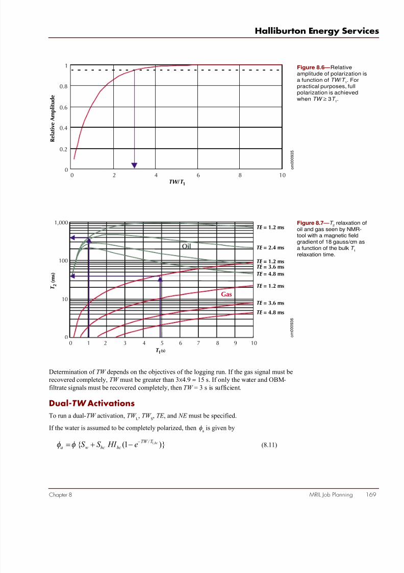
7/28/2019 NMR Logging Principles and Applications
http://slidepdf.com/reader/full/nmr-logging-principles-and-applications 187/253
MRIL Job Planning 16
Halliburton Energy Service
Chapter 8
Figure 8.6 —Relativeamplitude of polarization isa function of TW / T
1. For
practical purposes, fullpolarization is achieved
when TW ≥ 3T 1.
Figure 8.7 —T 2
relaxation ofoil and gas seen by NMR-tool with a magnetic fieldgradient of 18 gauss/cm asa function of the bulk T
1
relaxation time.
0
0.2
0.4
0.6
0.8
1
0 2 4 6 8 10TW /T 1
R e l a t i v e A m p l i t u d
e
T 1(s)
T 2 ( m s )
TE = 1.2 ms
TE = 2.4 ms
TE = 1.2 msTE = 3.6 ms
TE = 4.8 ms
TE = 1.2 ms
TE = 3.6 ms
TE = 4.8 ms
1,000
100
10
00 1 2 3 4 5 6 7 8 9 10
Oil
Gas
o m
0 0 0 9 3 5
o m
0 0 0 9 3 6
Determination of TW depends on the objectives of the logging run. If the gas signal must berecovered completely, TW must be greater than 3x4.9 ≈ 15 s. If only the water and OBM-filtrate signals must be recovered completely, then TW = 3 s is sufficient.
Dual-TW ActivationsTo run a dual-TW activation, TW
L, TW
S, TE , and NE must be specified.
If the water is assumed to be completely polarized, then φa
is given by
)1( ,1/ hcT TW
hchcwa e HI S S −−+=φφ (8.11)

7/28/2019 NMR Logging Principles and Applications
http://slidepdf.com/reader/full/nmr-logging-principles-and-applications 188/253
NMR Logging Principles and Applications
170 MRIL Job Planning Chapter 8
Equation 8.12 defines constants a, b, and c
)1,11
,1,1
,1
,1
≥≥≥
===
=
c b ,a(
T cT T baTW bTW
T aTW
whc
wS L
wS
(8.12)
Combining Eqs. 8.11 and 8.12 yields the apparent porosity measured at long- and short-wait times:
)1(
)1(
/
,
/
,
ca
hchcwS a
cba
hchcw La
e HI S S
e HI S S
−
⋅−
−+=
−+=
φφ
φφ
(8.13)
The differential signal, ∆φ, follows directly from subtracting the short TW signal from thelong TW .
To eliminate the response associated with the formation water from the differential signal,the water must be completely polarized at both short and long wait times. This condition ismet when TW
L ≈ TW
S ≈ 3 x T
1,water , or when a 3. (T
1,water ) is the longest T
1associated with
the pore water.)
)( // cbacahchc ee HI S −− −=∆ φφ (8.14)
For any given value of a greater than 3, the fraction of the full hydrocarbon signal residing inthe differential signal is a function of the dimensionless parameters b and c only, i.e. afunction of the ratio TW
Lto TW
Sand the ratio T
1,hcto T
1,w, which is the T
1contrast between
formation water and the hydrocarbon. This function is visualized in Fig. 8.8 for a = 3.
Example 1, Step 3: Determine Appropriate Activation Parameters(TW
L, TW
S, TE , NE ) for a Dual-TW Activation.
A dual-TW activation may also be selected for this example. Relevant T 1
relaxation times for this particular well are T
1,gas= 4.9 s, T
1,mf = 1.1 s and T
1, water ≈ 1 s (see Step 1 of this example),
indicating a gas-water T 1
contrast c = 4.9. Entering the chart in Fig. 8.8 at this contrastindicates that the maximum fraction of the gas signal can be in the 0.5 to 0.6 range; thearrows indicate how the most favorable ratio TW
L/ TW
Sof 5.5 is determined. That is 5.5
results in the smallest value of TW Lwhich results in a fractional gas signal in the 0.5 to 0.6
range. Adequate TW values are thus
TW S
= 3 T 1, water
= 3 s
TW L
=5.5 TW S
= 16.5 s
In the Step 2 of this example, the formation water signals were found to span the T 2
spectrumup to 400 ms, and the gas signal was expected to appear at 40 ms. The maximum relaxationtime to be resolved is 400 ms, which requires at least 400/(1.2 x 3) = 110 echoes.

7/28/2019 NMR Logging Principles and Applications
http://slidepdf.com/reader/full/nmr-logging-principles-and-applications 189/253
MRIL Job Planning 17
Halliburton Energy Service
Chapter 8
Figure 8.8 —The fractionof the completely polarizedhydrocarbon signal in thedifferential signal is afunction of the long-to-
short TW ratio (b) and ofthe hydrocarbon-water T
1
contrast (c). The short TW
is three times the longestT
1of the formation water
(i.e., a = 3) to ensure atleast 95% polarization offormation water.
1 2 3 4 5 6 7 8 9 101
2
3
4
5
6
7
8
9
10
b
a= 3
0.6-0.7
0.5-0.6
0.4-0.5
0.3-0.4
0.2-0.3
0.1-0.2
0.0-0.1
c
D e c i m a l F r a c t i o
n o f
C o m p l e t e l y P o l a r i z e d
H y d r o c a r b o n S i g n a l i n t h e
D i f f e r e n t i a l S i g n
a l
o m
0 0 0 9 3 7
The parameters for the dual-TW activation are thus
Activation 1: TE = 1.2 ms N = 110 TW L
= 16.5 s
Activation 2: TE = 1.2ms N = 110 TW S
= 3 s
This dual-TW activation maximizes the differential gas signal, but actual values of porosity,hydrocarbon saturation in the sensitive volume, and hydrogen index at in-situ conditionsdetermine whether this signal is sufficiently large to be detected at all.
Average net porosity in this well is about 14 p.u., the invaded-zone gas saturation is assumedat the residual level of 30%, and the hydrogen index of gas is 0.52 (see Step 1 of this ex-ample). Substituting these values into Eq. 8.14 gives
( ) p.u.ee 1.151.02.252.03.0149.4/5.169.4/3
=×=−××=∆−−
φ
This signal level is just above the detection limit for this technique and will appear at 40 msin the differential spectrum.
The whole process can be repeated to demonstrate that this dual-TW activation also effec-tively removes the flushed zone mud-filtrate signal (T
1, obmf = 1.1 s) from the differential
spectrum. When the filtrate T 1
increases, the outlined approach requires minor modification

7/28/2019 NMR Logging Principles and Applications
http://slidepdf.com/reader/full/nmr-logging-principles-and-applications 190/253
NMR Logging Principles and Applications
172 MRIL Job Planning Chapter 8
to determine the filtrate signal. The T 1
contrast between gas and OBM filtrate must be
evaluated to plan suitable TW values. This evaluation is demonstrated in Example 2.
Example 2: OBM, Dual TW
Well Description
An NMR job was planned for a well with the same reservoir properties as Example 1, but
with different properties of the OBM filtrate. As in Example 1, the well was a gas well, had
been drilled with OBM, had reached its target depth of 20,000 ft, and had maximum
bottomhole temperature and pressure of 8,700 psi and 300°F, respectively.
Step 1: Determine NMR Fluid Properties.
Gas and formation water properties are the same as the previous example. Also as in the
previous example, properties of the OBM filtrate were measured in the laboratory and
extrapolated to reservoir conditions. The pertinent gas, OBM filtrate, and formation-water
properties determined thus far are summarized in the first three data columns of Table 8.2.
Step 2: Assess Expected NMR Response.
The tabulated T 1 relaxation times are used in Eqs. 8.5 to 8.7 to compute the polarization as afunction of TW , shown in Fig. 8.9. The graph shows that full polarization of the formation
water, filtrate, and gas requires TW values of 3, 8, and 15 s, respectively. The T 2
values
logged by an MRIL tool with a magnetic field gradient of 18 gauss/cm and an echo spacing
of 1.2 ms, are determined from Fig. 8.7 and are tabulated under T 2D
in Table 8.2.
Step 3: Determine Appropriate Activation Parameters (TW L, TW
S, TE , NE ) for
a Dual-TW Activation.
Complete elimination of the formation-water and mud-filtrate signals from the differential
spectrum requires full polarization of both signals, imposing TW L
> TW S
> 8 s. The critical
ratio in this example is not the T 1
contrast between gas and water (i.e., c = 4.9), but instead
the T 1
contrast between gas and OBM filtrate (i.e., c = 2). Entering the chart in Fig. 8.8 at this
low contrast indicates that the fraction of the gas signal will not exceed the 0.2 to 0.3 range,
and the most suitable wait-time ratio TW L/TW
Sis 3.5. Thus, adequate TW values are
TW S
= 3 T 1, OBMF
= 8 s
TW L
=3.5 TW S
= 28 s
Table 8.2 indicates that the longest T 2
time logged in this well is 800 ms (OBM filtrate); the
number of echoes required to resolve this signal is at least 800/(1.2 x 3) = 220.
Gas
OBM-filtrate
Formation Water
T 2D (ms)
40
800
< 400
T 1 (s)
4.9
2.5
< 1
Hl
0.52
1
1
D 0 (cm2 /s)
85 x 10-5
2 x 10⁻⁵
1 x 10⁻⁵
Table 8.2 —Example 2: NMR Fluid Properties at Reservoir Conditions
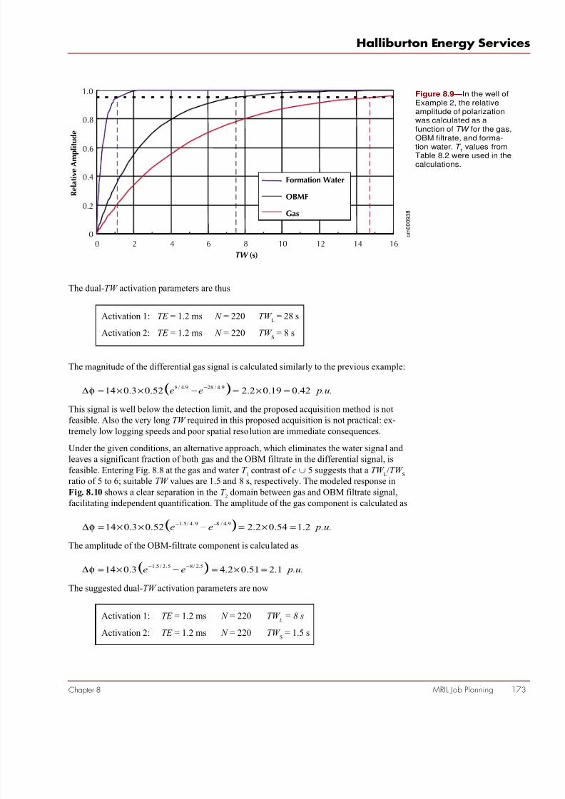
7/28/2019 NMR Logging Principles and Applications
http://slidepdf.com/reader/full/nmr-logging-principles-and-applications 191/253
MRIL Job Planning 17
Halliburton Energy Service
Chapter 8
The dual-TW activation parameters are thus
Activation 1: TE = 1.2 ms N = 220 TW L
= 28 s
Activation 2: TE = 1.2 ms N = 220 TW S
= 8 s
The magnitude of the differential gas signal is calculated similarly to the previous example:
( ) p.u.ee 42.019.02.252.03.0149.4/289.4/8
=×=−××=∆−
φ
This signal is well below the detection limit, and the proposed acquisition method is not
feasible. Also the very long TW required in this proposed acquisition is not practical: ex-tremely low logging speeds and poor spatial resolution are immediate consequences.
Under the given conditions, an alternative approach, which eliminates the water signal andleaves a significant fraction of both gas and the OBM filtrate in the differential signal, isfeasible. Entering Fig. 8.8 at the gas and water T
1contrast of c ∪ 5 suggests that a TW
L/TW
S
ratio of 5 to 6; suitable TW values are 1.5 and 8 s, respectively. The modeled response inFig. 8.10 shows a clear separation in the T
2domain between gas and OBM filtrate signal,
facilitating independent quantification. The amplitude of the gas component is calculated as
( ) p.u.ee 2.154.02.252.03.0149.4/89.4/5.1
=×=−××=∆−−
φ
The amplitude of the OBM-filtrate component is calculated as
( ) p.u.ee 1.251.02.43.0145.2/85.2/5.1
=×=−×=∆−−
φ
The suggested dual-TW activation parameters are now
Activation 1: TE = 1.2 ms N = 220 TW L
= 8 s
Activation 2: TE = 1.2 ms N = 220 TW S
= 1.5 s
Figure 8.9 —In the well ofExample 2, the relativeamplitude of polarizationwas calculated as afunction of TW for the gas,
OBM filtrate, and forma-tion water. T
1values from
Table 8.2 were used in thecalculations.
1.0
0
TW (s)
R e l a t i v e A m p l i t u d e
2 4 6 8 10 12 14 160
0.2
0.4
0.6
0.8
Formation Water
OBMF
Gas
o m
0 0 0 9 3 8

7/28/2019 NMR Logging Principles and Applications
http://slidepdf.com/reader/full/nmr-logging-principles-and-applications 192/253
NMR Logging Principles and Applications
174 MRIL Job Planning Chapter 8
Figure 8.10 —In Example 2,dual-TW acquisition with aTW
L / TW
Sratio of 28/8
(top three panels) elimi-nates the formation-water
and mud-filtrate signalsfrom the differentialspectrum and maximizesthe differential gas signal.However, the differentialsignals are small, andbecause of the longacquisition time, loggingspeeds are very slow.Alternatively, dual-TW
acquisition with TW L / TW
S
ratio of 8/1.5 (bottom twopanels) eliminates only theformation water from thedifferential spectrum, butthe gas and OBM-filtrate
signals are sufficientlyseparated in T
2space to
enable independentquantification.
w
Formation water OBMF GasTW L = 28 (s) TE = 1.2 (ms)
Formation water OBMF Gas
Formation water OBMF Gas
Formation water OBMF Gas
Formation ater OBMF Gas
1T 2 (ms)
100010010
1T 2 (ms)
100010010
1T 2 (ms)
100010010
1T 2 (ms)
100010010
1T 2 (ms)
100010010
TW S = 8 (s) TE = 1.2 (ms)
Differential Spectrum;TW = 28 and 8 (s)
TW S = 1.5 (s) TE = 1.2 (ms)
Differential Spectrum;TW = 8 and 1.5 (s)
o m
0 0 1 4 3 8
Dual-TE Activations
To run a dual-TE activation, TE L, TE
S, TW , and NE must be specified.
The marginal T 1
contrast between the OBM filtrate and the natural gas in Example 2 hin-dered differentiation of these fluids through the dual-TW method. However, the largeseparation of the gas and mud filtrate signals in the T
2domain, a reflection of the significant
diffusivity contrast in diffusivity between the two fluids, enabled quantitative determination
of the fluid volumes. More generally, if the diffusivity contrast is not sufficient to establishdifferentiation in the spectral domain when the data have been acquired under standardconditions, then the apparent contrast can be enhanced by acquiring data at increased TE (seeFig. 8.3).
Example 3: WBM, Viscous Oil, Dual TE
Well Description
A well was to be drilled with a water-based mud system in a viscous-oil reservoir.

7/28/2019 NMR Logging Principles and Applications
http://slidepdf.com/reader/full/nmr-logging-principles-and-applications 193/253
MRIL Job Planning 17
Halliburton Energy Service
Chapter 8
Step 1: Determine NMR Fluid Properties.
The relevant fluid properties are summarized in Table 8.3. The NMR properties of the water- based-mud filtrate are identical to those of the formation water. Note that the formation-water T
1is shorter than its bulk value and is not single-valued but a distribution, reflecting the pore-
size distribution of the rock. The T 1 value listed in the table is the logarithmic mean of this T 1distribution.
Step 2: Assess Expected NMR Response.
The tabulated T 1
relaxation times are used in Eqs. 8.5 to 8.7 to compute the polarization as afunction of TW , shown in Fig. 8.11. The T
2responses of the individual components are shown
in Fig. 8.12 (where a magnetic field gradient of 18 gauss/cm) for various values of TE .
Step 3: Determine Appropriate Activation Parameters (TE L, TE S, TW, and NE )for a Dual-TE Activation.
Inspection of Figs. 8.11 and 8.12 already indicates that standard T 2
logs and dual-TW logswill not be sufficient to differentiate fluids and to determine volumes. With a standardTE = 1.2 ms activation, all fluids present will have comparable T
2relaxation times (300 to
500 ms). Variation of the TW will reduce the WBM-filtrate signal and the oil signal equally,eliminating both from the differential spectrum.
Eqs 8.3 and 8.4 can be used to evaluate the difference in apparent T 2 as a function of TE for the “free” water and oil in this well. The results, summarized in Fig. 8.12, indicate completeseparation of the oil signal from the water at echo spacings in excess of 4.8 ms because of the
Crude Oil
Formation Water
T 2D (ms)
486
< 400
T 1 (s)
0.5
< 0.8
Hl
1
1
D 0 (cm2 /s)
0.2 x 10⁻⁵
1 x 10⁻⁵
Table 8.3 —Example 3: NMR Fluid Properties at Reservoir Conditions
WBMF
Oil
0TW (s)
1 2 3 4
1.0
R e l a t i v e A m p l i t u d e
0
0.2
0.4
0.6
0.8
Figure 8.11 —In the wellof Example 3, the relativeamplitude of polarizationwas calculated as afunction of TW for thecrude oil, water-basedmud filtrate, and formationwater. T
1values from
Table 8.3 were used in
the calculations. Thefiltrate and formationwater share bulk NMRproperties, and thus theircorresponding curves onthis graph are identical.
o m
0 0 1 4 3 9

7/28/2019 NMR Logging Principles and Applications
http://slidepdf.com/reader/full/nmr-logging-principles-and-applications 194/253
NMR Logging Principles and Applications
176 MRIL Job Planning Chapter 8
1T 2 (ms)
100010010
1T 2 (ms)
100010010
1T 2 (ms)
100010010
1T 2 (ms)
100010010
1T 2 (ms)
100010010
TW = 3 (s) TE = 1.2 (ms) Formation Water WBMF Oil
TW = 3 (s) TE = 2.4 (ms) Formation Water WBMF Oil
TW = 3 (s) TE = 3.6 (ms) Formation Water WBMF Oil
TW = 3 (s) TE = 4.8 (ms) Formation Water WBMF Oil
TW = 3 (s) TE = 6 (ms) Formation Water WBMF Oil
Figure 8.12 —In Example3, the T
2responses of the
formation water, oil, andwater-based mud filtrateshift to lower values as TE
increases. The apparentT
2of oil “lags” behind the
responses of the other twofluids because of the oil’slower diffusivity.
o m
0 0 1 4 4 0
difference in diffusivity between the two fluids. The greater diffusivity of the water com- pared to the oil induces enhanced shortening of the apparent T
2response at increasing echo
spacing.
Analogous to the previous examples, the appropriate number of echoes to resolve even theslowest components (T
2~ 800 ms) with a standard echo-spacing is 800/(1.2 x 3) = 220.
Increasing the spacing to 4.8 ms reduces the required number of echoes by the same factor to220/4 = 55. The suggested dual-TE activation parameters are thus
Activation 1: TE S
= 1.2 ms NE = 220 TW = 3 s
Activation 2: TE L
= 4.8 ms NE = 55 TW = 3 s
To run a dual-TW , dual-TE activation set, TE L , TE
S , TW
L , TW
S , and N must be specified.
˜
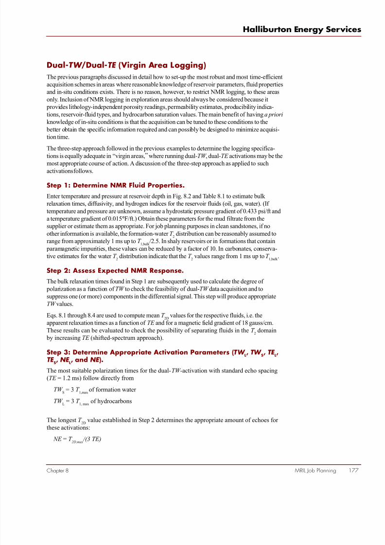
7/28/2019 NMR Logging Principles and Applications
http://slidepdf.com/reader/full/nmr-logging-principles-and-applications 195/253
MRIL Job Planning 17
Halliburton Energy Service
Chapter 8
Dual-TW /Dual-TE (Virgin Area Logging)
The previous paragraphs discussed in detail how to set-up the most robust and most time-efficientacquisition schemes in areas where reasonable knowledge of reservoir parameters, fluid propertiesand in-situ conditions exists. There is no reason, however, to restrict NMR logging, to these areasonly. Inclusion of NMR logging in exploration areas should always be considered because it
provides lithology-independent porosity readings, permeability estimates, producibility indica-tions, reservoir-fluid types, and hydrocarbon saturation values. The main benefit of having a priori
knowledge of in-situ conditions is that the acquisition can be tuned to these conditions to the better obtain the specific information required and can possibly be designed to minimize acquisi-tion time.
The three-step approach followed in the previous examples to determine the logging specifica-tions is equally adequate in “virgin areas,” where running dual-TW , dual-TE activations may be themost appropriate course of action. A discussion of the three-step approach as applied to suchactivations follows.
Step 1: Determine NMR Fluid Properties.
Enter temperature and pressure at reservoir depth in Fig. 8.2 and Table 8.1 to estimate bulk relaxation times, diffusivity, and hydrogen indices for the reservoir fluids (oil, gas, water). (If temperature and pressure are unknown, assume a hydrostatic pressure gradient of 0.433 psi/ft anda temperature gradient of 0.015°F/ft.) Obtain these parameters for the mud filtrate from thesupplier or estimate them as appropriate. For job planning purposes in clean sandstones, if noother information is available, the formation-water T
2distribution can be reasonably assumed to
range from approximately 1 ms up to T 1,bulk
/2.5. In shaly reservoirs or in formations that contain paramagnetic impurities, these values can be reduced by a factor of 10. In carbonates, conserva-tive estimates for the water T
2distribution indicate that the T
2values range from 1 ms up to T
1,bulk .
Step 2: Assess Expected NMR Response.
The bulk relaxation times found in Step 1 are subsequently used to calculate the degree of
polarization as a function of TW to check the feasibility of dual-TW data acquisition and tosuppress one (or more) components in the differential signal. This step will produce appropriateTW values.
Eqs. 8.1 through 8.4 are used to compute mean T 2D
values for the respective fluids, i.e. theapparent relaxation times as a function of TE and for a magnetic field gradient of 18 gauss/cm.These results can be evaluated to check the possibility of separating fluids in the T
2domain
by increasing TE (shifted-spectrum approach).
Step 3: Determine Appropriate Activation Parameters (TW L, TW
S, TE
L,
TE S, NE
L, and NE ).
The most suitable polarization times for the dual-TW -activation with standard echo spacing(TE = 1.2 ms) follow directly from
TW S
= 3 T 1,max
of formation water
TW L
= 3 T 1, max
of hydrocarbons
The longest T 2D
value established in Step 2 determines the appropriate amount of echoes for these activations:
NE = T 2D,max
/(3 TE)
7/28/2019 NMR Logging Principles and Applications
http://slidepdf.com/reader/full/nmr-logging-principles-and-applications 196/253
NMR Logging Principles and Applications
178 MRIL Job Planning Chapter 8
To utilize diffusion contrasts, an additional set of activations should be acquired with a longer
TE (e.g., 4.8 ms) and a corresponding number of echoes. Integrated interpretation of all data
thus acquired will reveal both formation and fluid properties.
Example 4: OBM, Gas, Dual TW, TE
Well Descr iption
High gas readings were observed while drilling an exploration well in an oil prospect,
indicating a small gas-cap. Cuttings showed sandstone and some shale. The well, drilled with
an OBM system, reached a depth of 12,000 ft, and no indications of any pressure or tempera-
ture anomalies were observed.
Step 1: Determine NMR Fluid Properties.
The temperature and pressure at reservoir depth are estimated at 12,000 x 0.015 = 180°F
(355° K) and 12,000 x 0.433 = 5,196 psi, respectively. Extrapolation of the laboratory-
measured mud-filtrate properties to reservoir conditions gives
)(5.1,1
sT mf
=
( ) scm D mf /1092.0 25,0
−×=
1=mf HI
The density of the gas at 180°F and 5,196 psi, read off Fig. 8.2 is 0.21 g/cm3. The other gas
properties are calculated using the equations listed in Table 8.1:
)(4.5355
21.0105.2105.2
17.1
4
17.1
4
ga,1 s T
T s =×=×=
ρ
( ) scmT D /108021.0
355105.8105.8259.029.02
gas,0
−−−×=×=×=
ρ
47.021.025.225.2gas =×== ρ HI
From experience in the area, the reservoir hydrocarbon liquid is most likely black oil with low
gas/oil ratio and with viscosity about 3 cp. With this information, the equations in Table 8.1
provide the water and oil properties:
)(84.03298
3553
2983oil,1 s
T T =
×
×
==
η
( ) scmT
D /1052.03298
3553
2983.1 25
oil,0
−×=×
×==
η
)(6.31298
3553
2983
water ,1 s
T T =
×
×
==
η

7/28/2019 NMR Logging Principles and Applications
http://slidepdf.com/reader/full/nmr-logging-principles-and-applications 197/253
MRIL Job Planning 17
Halliburton Energy Service
Chapter 8
OBM Filtrate
Gas
Oil
Formation Water
T 2 (ms)
500
45
325
< 400
T 1 (s)
1.5
5.4
0.84
< 1
Hl
1
0.47
1
1
D 0 (cm2 /s)
0.92 x 10⁻⁵
80 x 10-5
0.52 x 10⁻⁵
1.5 x 10⁻⁵
( ) scmT
D /105.11298
3553
2983.1 25
water ,0
−×=×
×==
η
1water oil≈≈ HI HI
The NMR fluid properties for this well are summarized as Table 8.4.
Step 2: Assess Expected NMR Response.
The bulk relaxation times established in Step 1 are subsequently used to compute the polarization curves presented in Fig. 8.13. Note that surface-relaxivity and pore sizes shortenthe formation water T
1well below its bulk value, and the observed relaxation time is not
single-valued but a distribution, reflecting the pore-size distribution of the rock. The T 1
value
listed in the table is the logarithmic mean of this T 1 distribution.Eqs. 8.1 through 8.4 have also been used to compute the typical T
2responses of these fluids
at various TE values, shown in Fig. 8.14.
Table 8.4 —Example 4: NMR Fluid Properties at Reservoir Conditions
(TE = 1.2 ms, G = 18 gauss/cm)
Figure 8.13 —In theexploration well of Ex-ample 4, the relativeamplitude of polarizationwas calculated as afunction of TW for the gas,oil, formation water, andOBM filtrate. T
1values
from Table 8.4 were usedin the calculations.
o m
0 0 1 4 4 1
1.0
R e l a t i v e A
m p l i t u d e
0
0.2
0.4
0.6
0.8
0TW (s)
5 10 15 20
Formation Water
OBMF
Oil
Gas

7/28/2019 NMR Logging Principles and Applications
http://slidepdf.com/reader/full/nmr-logging-principles-and-applications 198/253
NMR Logging Principles and Applications
180 MRIL Job Planning Chapter 8
Step 3: Determine Appropriate Activation Parameters (TW i, TE
i, NE
i).
Inspection of the table and figures computed for the fluids in this exploration well shows thatthe slowest component relaxes at T
2= a rate of some 500 ms (OBMF at TE = 1.2 ms). The
appropriate number of echoes to resolve even these slow components is
NE = 500 / (3 x 1.2) ≈ 133
The big T 1
contrast between gas and all other fluids calls for differential spectrum or differ-ential echo analysis (time domain analysis). Adequate TW values are 16 and 5 s.
The NMR properties of the native oil and the OBM filtrate are very similar. Any pair of dual-TW data will reduce both components at about equal rates. Acquiring data TE = 6 ms at TW =5 s and TW = 1.5 s offers the possibility to eliminate the water signal from this diffusiondata, which may simplify the interpretation.
Figure 8.14 —These T 2
responses at various TE
values were calculated forthe formation water, oil,gas, and OBM filtrate from
the exploration well ofExample 4.
TE = 1.2 (ms)
1T 2 (ms)
100010010
1T 2 (ms)
100010010
1T 2 (ms)
100010010
1T 2 (ms)
100010010
1T 2 (ms)
100010010
OBMF OilFormation Water Gas
OBMF OilFormation Water Gas
OBMF OilFormation Water Gas
OBMF OilFormation Water Gas
OBMF OilFormation Water Gas
TE = 2.4 (ms)
TE = 3.6 (ms)
TE = 4.8 (ms)
TE = 6 (ms)
o m
0 0 1 4 4 2
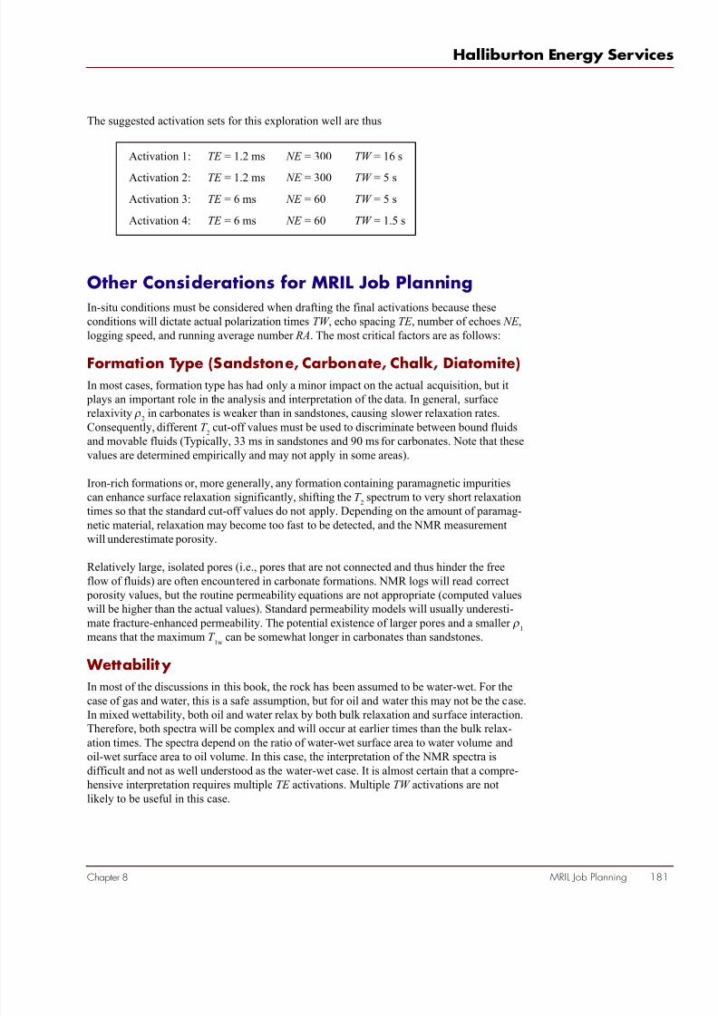
7/28/2019 NMR Logging Principles and Applications
http://slidepdf.com/reader/full/nmr-logging-principles-and-applications 199/253
MRIL Job Planning 18
Halliburton Energy Service
Chapter 8
The suggested activation sets for this exploration well are thus
Activation 1: TE = 1.2 ms NE = 300 TW = 16 s
Activation 2: TE = 1.2 ms NE = 300 TW = 5 s
Activation 3: TE = 6 ms NE = 60 TW = 5 s
Activation 4: TE = 6 ms NE = 60 TW = 1.5 s
Other Considerations for MRIL Job Planning
In-situ conditions must be considered when drafting the final activations because theseconditions will dictate actual polarization times TW , echo spacing TE , number of echoes NE ,logging speed, and running average number RA. The most critical factors are as follows:
Formation Type (Sandstone, Carbonate, Chalk, Diatomite)
In most cases, formation type has had only a minor impact on the actual acquisition, but it plays an important role in the analysis and interpretation of the data. In general, surfacerelaxivity ρ
2in carbonates is weaker than in sandstones, causing slower relaxation rates.
Consequently, different T 2
cut-off values must be used to discriminate between bound fluidsand movable fluids (Typically, 33 ms in sandstones and 90 ms for carbonates. Note that thesevalues are determined empirically and may not apply in some areas).
Iron-rich formations or, more generally, any formation containing paramagnetic impuritiescan enhance surface relaxation significantly, shifting the T
2spectrum to very short relaxation
times so that the standard cut-off values do not apply. Depending on the amount of paramag-netic material, relaxation may become too fast to be detected, and the NMR measurementwill underestimate porosity.
Relatively large, isolated pores (i.e., pores that are not connected and thus hinder the freeflow of fluids) are often encountered in carbonate formations. NMR logs will read correct
porosity values, but the routine permeability equations are not appropriate (computed valueswill be higher than the actual values). Standard permeability models will usually underesti-mate fracture-enhanced permeability. The potential existence of larger pores and a smaller ρ
1
means that the maximum T 1w
can be somewhat longer in carbonates than sandstones.
Wettability
In most of the discussions in this book, the rock has been assumed to be water-wet. For thecase of gas and water, this is a safe assumption, but for oil and water this may not be the case.
In mixed wettability, both oil and water relax by both bulk relaxation and surface interaction.Therefore, both spectra will be complex and will occur at earlier times than the bulk relax-ation times. The spectra depend on the ratio of water-wet surface area to water volume andoil-wet surface area to oil volume. In this case, the interpretation of the NMR spectra isdifficult and not as well understood as the water-wet case. It is almost certain that a compre-hensive interpretation requires multiple TE activations. Multiple TW activations are notlikely to be useful in this case.
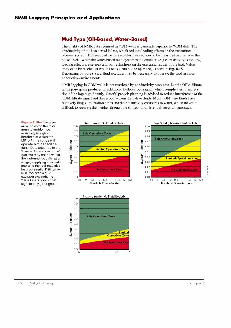
7/28/2019 NMR Logging Principles and Applications
http://slidepdf.com/reader/full/nmr-logging-principles-and-applications 200/253

7/28/2019 NMR Logging Principles and Applications
http://slidepdf.com/reader/full/nmr-logging-principles-and-applications 201/253
96
80
64
48
32
16
0
0.01 0.1 1 10
Resistivity of 8 1/2-in. Borehole (ohm-m)
R u n n i n g A v e r a g e
6
0 1 2 3 4 5 6 7 8 9 10 11 12 13 14 15 16
2
5
4
3 V e r t i c a l R e s o l u t i o n
( f t )
Logging Speed (ft/min)
R u n n i n g
A v e r a
g e = 1
6
R u n n i n
g A v e r a g e
= 3 2
R u n n i n
g A
v e r a
g e = 9 6
R u n n i n
g A v e r a g e =
4 8
R u n n i n
g A
v e r a
g e
= 8
0
R u n n i n
g A v e r a
g e
= 6 4
Figure 8.16— This speed-chart applies for the MAX4MRIL-Prime activation.Entering the left chart withR
mgives the number of
running averages to beused. The intercept of thecorresponding trend linein the bottom graph withthe desired verticalresolution indicates thelogging speed.
o m
0 0 1 4 4
4
Trade Off Logging Speed ⇔ Accuracy (S/N , Sampling Rate) ⇔Type and Detail of Information
When planning the drilling of any well, the logging program must be given some attention.
S/N is primarily controlled by borehole size and mud resistivity. As S/N decreases, the
running average ( RA) needed to maintain a specified error in porosity increases. The general practice is to require that the porosity have no more than one porosity unit standard devia-
tion. The value of RA combined with the logging speed determines the vertical resolution.
These relationships are summarized for the MRIL-Prime MAX4-activation in Fig. 8.16. The
figure clearly indicates that mud resistivity has great impact on the maximum logging speed.
The value RA increases exponentially when Rm
falls below 0.1 ohm-m; the associated drastic
decrease in logging speed is evident.
Relaxing vertical resolution in less interesting zones or over homogeneous intervals helps to
speed up logging. The same holds for the NMR specific requirements: high precision and
accuracy enforce slow-logging operations. For the most common activations, methods have
been developed that allow higher logging speeds and only marginally compromise the outcome.
MRIL Job Planning 183
Halliburton Energy Service
Chapter 8

7/28/2019 NMR Logging Principles and Applications
http://slidepdf.com/reader/full/nmr-logging-principles-and-applications 202/253
NMR Logging Principles and Applications
184 MRIL Job Planning Chapter 8
References
1. Akkurt, R., et al., 1995, NMR logging of natural gas reservoirs, paper N, 36 th Annual
SPWLA Logging Symposium Transactions, 12 p.
2. Prammer, M.G., et al., 1995, Lithology-independent gas detection by gradient-NMR logging, SPE 30562, presented at the 1995 SPE Annual Technical Conference andExhibition, 12 p.
3. Akkurt, R., et al., 1998, Enhanced Diffusion: Expanding the range of NMR direct hydro-carbon-typing Applications, paper GG, presented at the 39th Annual SPWLA Logging
Symposium, 14 p.
4. Vinegar, H.J., 1995, Short course notes, SPWLA short course on NMR, Houston, Texas.
5. Log Interpretation Principles/Applications, 1987, Schlumberger Educational Services,Houston, Texas, p. 45.
6. Gerritsma, C.J., Oosting, P.H., and Trappeniers, N.J., 1971, Proton spin-lattice relaxation
and self-diffusion in methanes: II. Experimental results for proton spin-lattice relaxationtimes, Physica, v. 51, p. 381–394.
7. Oosting, P.H., and Trappeniers, N.J., 1971, Proton spin-lattice relaxation and self-diffusionin methanes: IV. Self-diffusion in methanes, Physica, v. 51, p. 418–431.
8. Dawson, R., Khory, F., and Kobayashi, R., 1970, Self-diffusion measurements in methane by pulsed nuclear magnetic resonance: AlChE Journal , v. 16, no. 5, p. 725–729.
9. Zhan, Q., et al., 1998, Some exceptions to default NMR rock and fluid properties, paper FF, 39th Annual SPWLA Logging Symposium Transactions, 14 p.
10. Yarborough, L., and Hall, K.R., Oil & Gas Journal , Feb. 1974, p. 86.
11. Craig, F.F., The Reservoir Engineering Aspects of Water Flooding, SPE Monograph
Volume 3 of the Henry L. Doherty series, Dallas, 1993, p. 12.12. Kleinberg, R.L., et al., 1993, Nuclear Magnetic Resonance of Rocks: T
1vs. T
2, SPE
26470, presented at the 1993 SPE Annual Technical Conference and Exhibition, 11 p.
13. Prammer, M.G., et al., 1999, Theory and operation of a new, multivolume NMR loggingsystem, paper DD, presented at the 40th Annual SPWLA Logging Symposium, 12 p.
14. McCain Jr., W. D., 1990, Petroleum Fluids, Pennwell Books, Tulsa, Oklahoma, p. 330–331.
7/28/2019 NMR Logging Principles and Applications
http://slidepdf.com/reader/full/nmr-logging-principles-and-applications 203/253
MRIL Log Quality Control 185
Halliburton Energy Services
Chapter 9
MRIL LogQuality Control
Chapter 9
Quality control is essential to obtaining accurate information for the
MRIL log. A system of tool-integrity and log-quality indicators is used
to ensure the highest level of data quality. The MRIL quality-control
procedure includes calibration, verification (before-survey and after-
survey), operational setup, log recording, display of quality indicators,
and a final quality check. This chapter is divided into five sections:
concepts and definitions needed to understand the log quality assur-
ance discussion, calibration and verification, quality control duringlogging, logging quality display, and post-logging quality check.
Concepts and Definitions
Gain and Q Level
Gain indicates the amount of loading applied to the MRIL tool’s
transmitter circuit by borehole fluids and formation. Gain is measured
in real time by using a test coil (B1
coil) built into the tool. The test coil
transmits an RF signal, which is received by the RF antenna. Gain is
the ratio of the amplitude of the signal induced in the RF antenna
divided by the amplitude of the signal in the test coil. A gain measure-
ment is made as a part of each pulse sequence.
Gain is frequency-dependent. The operating frequency of a tool should
be set to achieve maximum gain.
Gain measured when the tool is in the borehole includes effects caused
by both the external environment and the transmitter circuit itself.
External factors that affect gain are primarily the borehole fluid
resistivity and, to a lesser degree, formation resistivity. Low-resistivity
muds or formations produce greater signal attenuation than high-
resistivity muds or formations, and thus result in lower gain. Because
borehole fluid resistivity does not change drastically over typical
logging intervals, changes in gain are usually the result of changes in
formation resistivity or borehole size when conductive mud is used.
Gain should never be zero. Sudden changes or spikes in gain usually
indicate tool problems.
MRIL activations are designed to run at a certain Q level: high Q,
medium Q, or low Q. The gain value determines which Q level to use,
as indicated in Table 9.1.

7/28/2019 NMR Logging Principles and Applications
http://slidepdf.com/reader/full/nmr-logging-principles-and-applications 204/253
NMR Logging Principles and Applications
186 MRIL Log Quality Control Chapter 9
Table 9.1 —Q -Level Determination
B1and B
1mod
B1
is the strength of the CPMG pulse that produces proton tipping and re-phasing. As a part
of every pulse sequence, B1
is measured using the test coil. The B1
curve should be relatively
constant but should show some variation with changes in borehole and formation conductiv-
ity. B1
will decrease across conductive washouts and conductive formations. Changes in the
B1
values should vary together with gain in the same direction following changes in total
conductivity.
The value of B1
corrected for borehole temperature is called B1mod
. The relation between B1mod
and B1
is given by:
)](0033.01[1mod 1 ncalibratiomagnet T T B B −+= (9.1)
where T magnet
is the temperature of the magnet at downhole conditions, and T calibration
is the
temperature of the magnet in the calibration tank during calibration. Both temperatures are
expressed in degrees Centigrade.
To give the maximum signal value during logging, B1
must be controlled so that B1mod
remains
within 5% of the peak value determined during shop calibration. If B1mod
does not remain in
this range, then the following effects occur:
•Protons will be under- or over-tipped.
• The signal-to-noise ratio for the tool and the precision of the porosity measurement
will decrease.
Any sudden change or spikes on the B1mod
curve usually indicate tool problems and should be
investigated.
Chi
Chi is a measure of the quality of fit between the calculated decay curve and the recorded
echo amplitudes. Chi is one of the primary log quality indicators monitored during logging.
In general, the value of Chi should be less than 2, but in certain low-Q situations, it may
average slightly higher than 2. Sudden changes or spikes in Chi usually indicate tool prob-
lems and should be investigated, even if Chi remains below 2.
Noise Indicators: OFFSET, NOISE, RINGING, and IENoise Noise for each CPMG experiment is described by four noise measures: offset (OFFSET ),
noise ( NOISE ), ringing ( RINGING ), and inter-echo noise ( IENoise), as shown in Fig. 9.1.
Gain
>300
200 - 300
<200
Q Level
high Q
medium Q
low Q
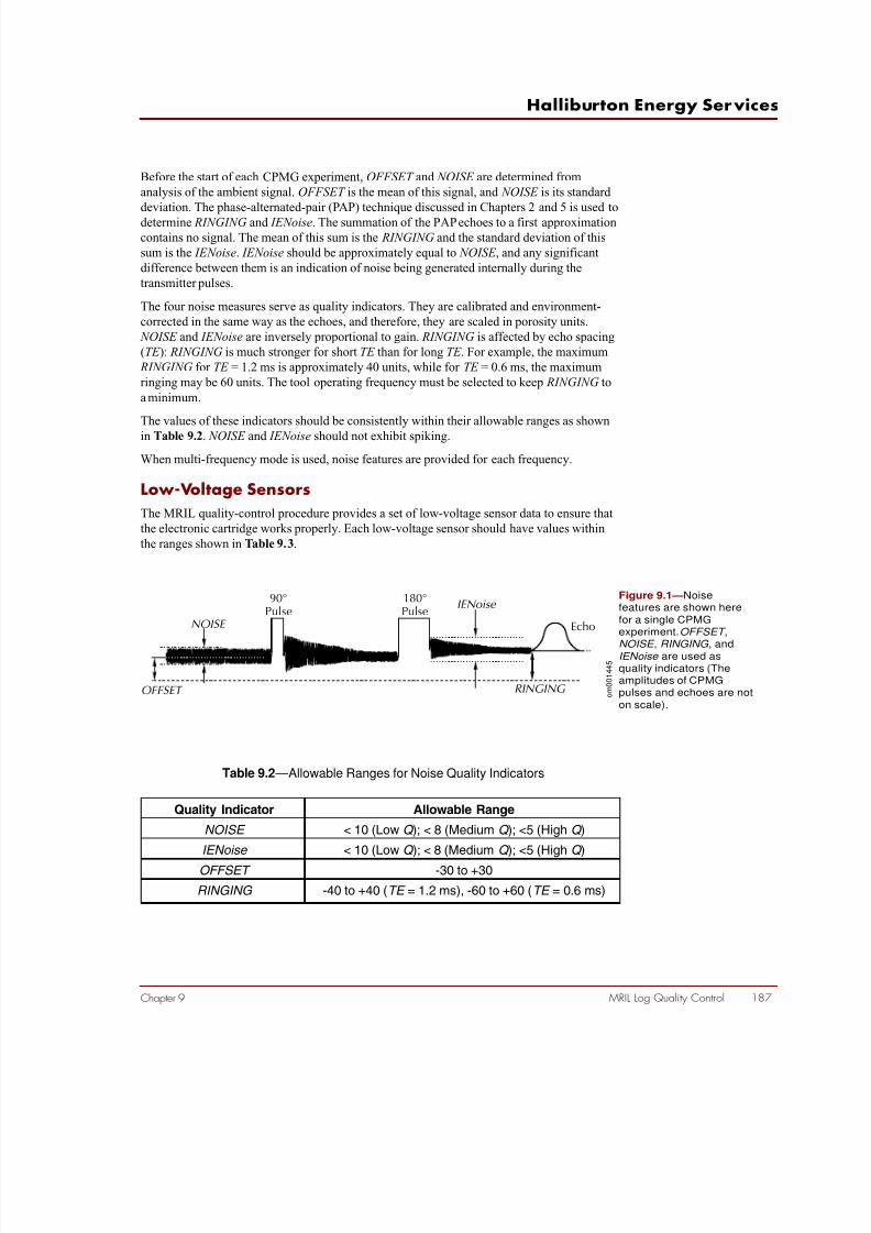
7/28/2019 NMR Logging Principles and Applications
http://slidepdf.com/reader/full/nmr-logging-principles-and-applications 205/253
MRIL Log Quality Control 187
Halliburton Energy Services
Chapter 9
Before the start of each CPMG experiment, OFFSET and NOISE are determined from
analysis of the ambient signal. OFFSET is the mean of this signal, and NOISE is its standard
deviation. The phase-alternated-pair (PAP) technique discussed in Chapters 2 and 5 is used to
determine RINGING and IENoise. The summation of the PAP echoes to a first approximation
contains no signal. The mean of this sum is the RINGING and the standard deviation of this
sum is the IENoise. IENoise should be approximately equal to NOISE , and any significant
difference between them is an indication of noise being generated internally during the
transmitter pulses.
The four noise measures serve as quality indicators. They are calibrated and environment-
corrected in the same way as the echoes, and therefore, they are scaled in porosity units.
NOISE and IENoise are inversely proportional to gain. RINGING is affected by echo spacing
(TE ): RINGING is much stronger for short TE than for long TE . For example, the maximum
RINGING for TE = 1.2 ms is approximately 40 units, while for TE = 0.6 ms, the maximum
ringing may be 60 units. The tool operating frequency must be selected to keep RINGING to
a minimum.
The values of these indicators should be consistently within their allowable ranges as shown
in Table 9.2. NOISE and IENoise should not exhibit spiking.
When multi-frequency mode is used, noise features are provided for each frequency.
Low-Voltage Sensors
The MRIL quality-control procedure provides a set of low-voltage sensor data to ensure that
the electronic cartridge works properly. Each low-voltage sensor should have values within
the ranges shown in Table 9.3.
Figure 9.1—Noisefeatures are shown here
for a single CPMGexperiment.OFFSET ,
NOISE ,
RINGING , and
IENoise are used asquality indicators (Theamplitudes of CPMGpulses and echoes are not
on scale).
NOISE
90°Pulse
180°Pulse
OFFSET
IENoise
RINGING
Echo
o m
0 0 1 4 4 5
Quality Indicator
NOISE
IENoise
OFFSET
RINGING
Allowable Range
< 10 (Low Q ); < 8 (Medium Q ); <5 (High Q )
< 10 (Low Q ); < 8 (Medium Q ); <5 (High Q )
-30 to +30
-40 to +40 (TE = 1.2 ms), -60 to +60 (TE = 0.6 ms)
Table 9.2 —Allowable Ranges for Noise Quality Indicators

7/28/2019 NMR Logging Principles and Applications
http://slidepdf.com/reader/full/nmr-logging-principles-and-applications 206/253
NMR Logging Principles and Applications
188 MRIL Log Quality Control Chapter 9
High-Voltage Sensors
The MRIL surface system attempts to maintain 600 VDC on the bank of capacitors that
provide the high current needed to produce CPMG pulses. Normally, the current transmitted
from the surface is insufficient to keep the capacitors fully charged during an echo train, and
as a result, the voltage output from the capacitors decreases during a CPMG echo train.
The MRIL tool can compensate for changes in voltage. The capacitor voltage is measured at
the beginning and at the end of the pulse (echo) train, and both values are reported in real
time. The voltage at the beginning of the cycle is defined as HVmax, and the voltage at the
end of the cycle is defined as HVmin.
In a high-Q environment with 50 echoes and TW ≥ 1500 ms, HVmax should be approxi-
mately the same as the voltage indicated on the voltage meter on the power-supply panel.
For standard T 2, dual-TW , and dual-TE activations, HVmin must remain above 400 VDC. If itdoes not, the tool will not be able to compensate for this reduced voltage and B
1will be
reduced. The reduction in B1
generally results in the porosity being underestimated, espe-
cially for the longer T 2
components.
When the total-porosity activation is used, two activation sets are run in tandem: a standard
T 2
activation to measure effective porosity and a partial polarization activation to measure
clay-bound water. In this case, because the partial-polarization activation immediately
follows the standard T 2
activation, the reported HVmin is not only the voltage at the end of
the CPMG for effective-porosity activation, but it is also the voltage at the beginning of the
CPMG for partial-polarization activation. Thus, when logging with total-porosity activation,
HVmin cannot be allowed to drop below 450 VDC.
Phase Correction Information: PHER , PHNO , and PHCO
The NMR signal from the antenna is fed into a phase-sensitive detector that outputs twochannels of data (Channel 1 and Channel 2) 90° apart. Data from both channels can be
plotted as a function of echo time, as shown in Fig. 9.2a for a single experiment and in Fig.
Table 9.3 —Low-Voltage Sensor Mnemonics and Data Ranges
Sensor Name
Ur 15 high
+15 Analog
-15 Analog
15 Trans
Ur 15 low
Unreg 5 v
+5 Analog
-5 Analog
+5 Digital
Real-Time-Display Mnemonic
15VUP
15V
15VN
15VT
15VUM
5VUM
5VA
5VAN
5VD
Data Range
1924
14.815.2
-14.8 -15.2
14.815.2
1924
9.512.5
4.95.1
-4.9 -5.1
4.95.1

7/28/2019 NMR Logging Principles and Applications
http://slidepdf.com/reader/full/nmr-logging-principles-and-applications 207/253
MRIL Log Quality Control 189
Halliburton Energy Services
Chapter 9
9.2b for eight stacked experiments. Data from both channels can also be crossplotted, as
shown in Fig. 9.3a for a single experiment and in Fig. 9.3.b for eight stacked experiments.
The magnitude of the echo train can be calculated as
)()()(22i E i E i E y xamp += (9.2)
where E amp(i) is the calculated amplitude for the ith echo, and E
x(i) and E
y(i) are the amplitudes
of the ith echo for Channels 1 and 2, respectively. However, this calculation is affected by
rectification, and all noises contribute as positive signals. Therefore, the decay curve never
goes to zero but stays at some small value, which echo fitting will convert to a long T 2
component.
The magnitude of the echo train can be calculated by a different approach to remove the
problem of noise rectification. This approach is designed to produce two channels of data:
one channel consists primarily of the NMR signal, which is to be used for further processing,
and the other channel consists primarily of noise with zero mean. In this approach, an angle ϕ
is calculated from
∑
∑
=
=−=
k
i
x
k
i
y
i E
i E
2
21
)(
)(
tanϕ(9.3)
where i is the ith echo in the echo train, and k is the number of echoes to be used for phase-
angle calculation. Typically, 2 ≤ k ≤ 9. This calculation is performed after a running average
has been applied. This angle is then applied to the data from both channels as a phase-
correction angle. This phase correction is equivalent to rotating the Channel 1 and Channel 2
data through an angle of ϕ. After rotation, one channel will contain primarily the NMR signal
(whose amplitude is the real part of the echo train), and the other channel will contain
primarily noise (whose amplitude is the imaginary part of the echo train), as shown in Fig.
9.4. The real part of the echo train is converted to a T 2
distribution.
PHER is the mean of the imaginary part of the echo train and is ideally is zero. In practice,
PHER should be less than one for good data. PHNO is the standard deviation of the imagi-
nary part of the echo train and should be comparable in size to the other noise indicators. In
addition, the calculated angle for phase correction, designated as PHCO, can be also dis-
played as a quality indicator. If the measured signal is too small, then PHCO will show
random changes with depth. If the measured signal has sufficient amplitude, then PHCO
should remain stable with depth. For dual-TW or dual-TE logging, PHCOA, which is the
PHCO for long TW or short TE , should be about the same as PHCOB, which is the PHCO for
short TW or long TE .
Temperature
Three temperature indicators are reported during logging: Temp1, Temp2, and Temp3.Temp1 is the temperature of the electronics cartridge flask, Temp2 is the temperature of the
transmitter module, and Temp3 is the temperature of the magnet.
E amp(i) = √ E 2 (i) + E y2 (i)
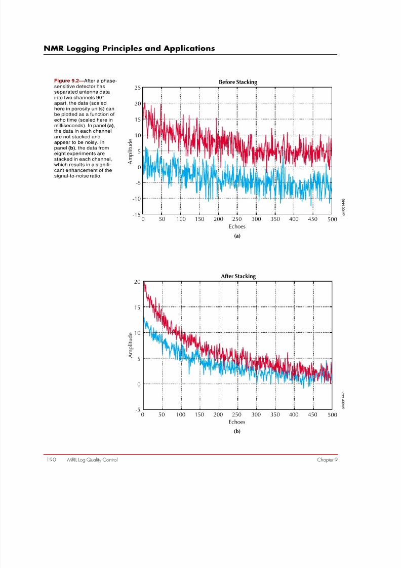
7/28/2019 NMR Logging Principles and Applications
http://slidepdf.com/reader/full/nmr-logging-principles-and-applications 208/253
NMR Logging Principles and Applications
190 MRIL Log Quality Control Chapter 9
Before Stacking
Amplitude
15
25
20
10
5
0
-5
-10
0 50 100 150 200 250 300 350 400 450 500-15
Echoes
(a)
15
20
10
5
0
-50 50 100 150 200 250 300 350 400 450 500
Echoes
(b)
After Stacking
Amplitude
Figure 9.2 —After a phase-sensitive detector hasseparated antenna data
into two channels 90°
apart, the data (scaledhere in porosity units) canbe plotted as a function of
echo time (scaled here inmilliseconds). In panel (a),the data in each channel
are not stacked andappear to be noisy. Inpanel (b), the data from
eight experiments arestacked in each channel,which results in a signifi-cant enhancement of the
signal-to-noise ratio.
o m
0 0 1 4 4 6
o m
0 0 1 4 4 7
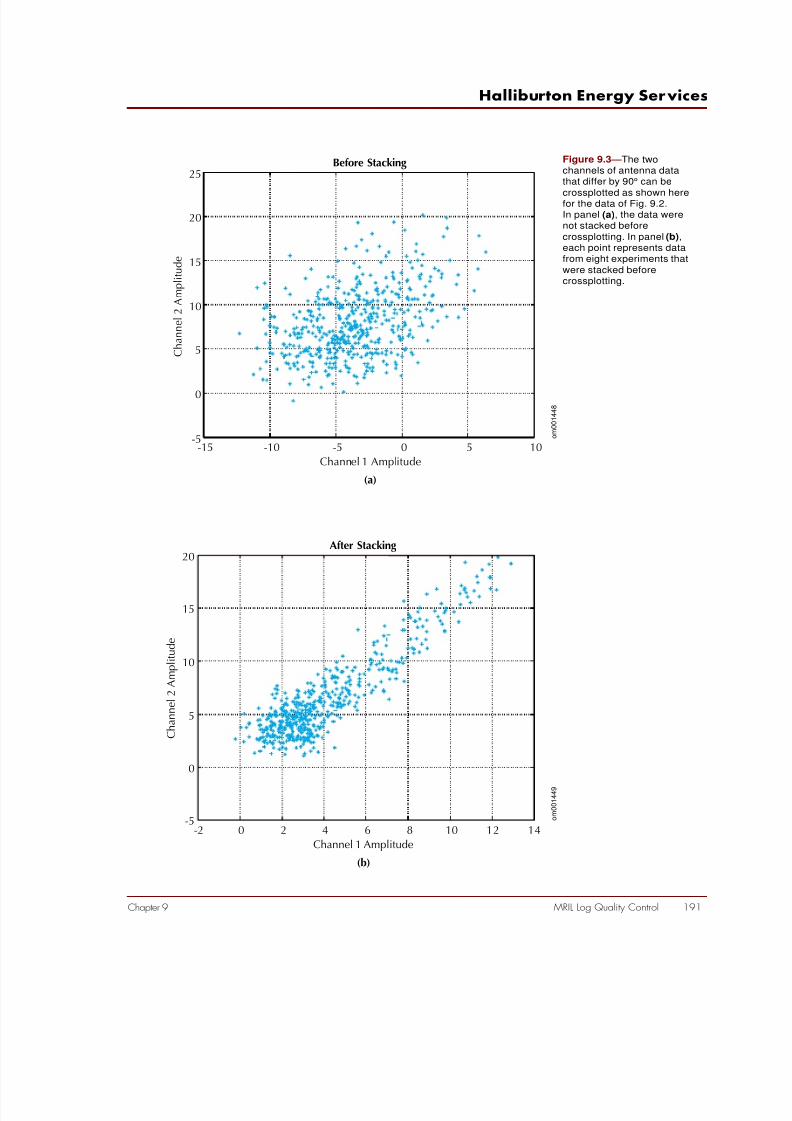
7/28/2019 NMR Logging Principles and Applications
http://slidepdf.com/reader/full/nmr-logging-principles-and-applications 209/253
MRIL Log Quality Control 191
Halliburton Energy Services
Chapter 9
Figure 9.3 —The twochannels of antenna datathat differ by 90° can be
crossplotted as shown herefor the data of Fig. 9.2.In panel (a), the data werenot stacked before
crossplotting. In panel (b),each point represents datafrom eight experiments that
were stacked beforecrossplotting.
Before Stacking
15
25
10
5
0
-5-15 -10 -5 0 5 10
Channel 1 Amplitude
(a)
20
Channel2Amplitude
After Stacking
10
20
5
0
-5-2 0 2 4 6 8 10 12 14
Channel 1 Amplitude
Channel2Amplitude
(b)
15
o m
0 0 1 4 4 8
o m
0 0 1 4 4 9

7/28/2019 NMR Logging Principles and Applications
http://slidepdf.com/reader/full/nmr-logging-principles-and-applications 210/253
NMR Logging Principles and Applications
192 MRIL Log Quality Control Chapter 9
After Phase Correction
15
25
10
0
-50 5 10 15 20 25
Channel 1 Amplitude
Channel2Amplitude
(b)
20
5
After Phase Correction
15
25
10
0
-50 50 100 150 200 250 300 350 400 450 500
Echoes
Amplitude
(b)
20
5
o m
0 0 1 4 5 0
o m
0 0 1 4 5 1
Figure 9.4 —Channel 1and Channel 2 data fromthe antenna can be rotated
to reduce the problem ofnoise rectification. Thebase data used here aresame as those used for
Figs. 9.2 and 9.3. Afterrotation, the crossplotteddata (a) from the two
channels will cluster arounda horizontal line corre-sponding to a Channel 2
amplitude of zero. Afterrotation, the amplitude ofthe Channel 1 data (b) isthe real part of the echo
train and is used for echofitting. After rotation, theamplitude of the Channel 2
data is the imaginary part
of the echo train.

7/28/2019 NMR Logging Principles and Applications
http://slidepdf.com/reader/full/nmr-logging-principles-and-applications 211/253
MRIL Log Quality Control 193
Halliburton Energy Services
Chapter 9
Pre-Logging Calibration and Verification
The MRIL tool is calibrated before every logging job in a calibration tank, as shown in Fig.
9.5. A complete calibration is not necessarily done before every logging job but is done at
least monthly. The calibration procedure must be done for each activation. The calibration
tank is made of fiberglass and is lined with a thin metallic coating. The tank serves as a
container for the water sample and as a Faraday cage to shield out unwanted background RF
signals. In its original form, the calibration tank had three chambers concentric with the axis
along which the antenna is placed. To calibrate the 6-in. tool, the outer chamber is filled with
water that has been doped with cupric sulfate. The cupric sulfate significantly reduces the T 1
relaxation time of water. With this setup, the sensitive volume contains 100% water, and
because the water has a relatively fast relaxation time, the calibration time is short. The
middle and inner chambers may be filled with waters of different salinity to simulate bore-
hole conditions. In the calibration of the 4˚-(C) and 4 7/8-(Prime) in. tools, the middle
chamber is filled with doped water, and the inner chamber may be filled with brine to
simulate antenna loading. Newer versions of the calibration tank contain only one chamber,
and a dummy load simulates borehole conditions.
The parameters determined during shop calibration are
• The pulse strength B1
need to produce the maximum A0, where A
0is the amplitude of
echo train at time zero. (Both 90° and 180° pulses have the same amplitude but
different lengths.)
• The relationship between B1
and A0
that is required to perform a “power correction.”
• The correction to Echoes 1 and 2, resulting from the so-called stimulated echo effect.
The relationship between A0 and porosity. (The maximum A
0is calibrated to 100% porosity in
the calibration tank.)
Formation Chamber
Borehole ChamberFaraday Cage
MRIL Tool
SensitiveVolumes
Side View End View Figure 9.5 —The cham-bers of this MRIL calibra-
tion tank are filled withdoped water to simulatethe borehole fluid and a
sensitive volume of100% porosity.
o m
0 0 1 4 5 2

7/28/2019 NMR Logging Principles and Applications
http://slidepdf.com/reader/full/nmr-logging-principles-and-applications 212/253
NMR Logging Principles and Applications
194 MRIL Log Quality Control Chapter 9
Calibration Procedure
The shop calibration procedure includes a frequency sweep test, a master calibration, and a
tank statistical check. Only the tank statistical check must be done before every logging job.
Frequency Sweep
A frequency sweep is performed to find a frequency at which the highest gain occurs. During
a frequency sweep, software is used to change the transmitter frequency over a fairly wide
range in the test coil while simultaneously measuring gain at the RF antenna. As the fre-
quency graph in Fig. 9.6 illustrates, a frequency can be found at which the maximum gain
occurs. The transmitter is then set to operate at this frequency.
A frequency sweep is essential for proper operation of the tool. The operating frequency
affects the tool’s transmitter and receiver circuits in two ways. First, if the transmitter and
receiver circuits are not tuned to the same frequency and power transmission is not efficient,
then the tool may overheat and become inoperable. Second, the efficiency of the receiver
circuit decreases sharply outside a very narrow frequency band centered on the resonant
frequency of the antenna. Consequently, if an incorrect operating frequency is selected, echoamplitudes are artificially reduced and the signal-to-noise ratio decreases. Likewise, if the
tool is calibrated at an incorrect frequency, subsequent logs will contain incorrect data.
Master Calibration
The master calibration determines the amplitude of the CPMG pulses as well as the relations
for power and stimulated-echo corrections1. The amplitudes E 1
and E 2
of Echo 1 and Echo 2,
respectively, are recorded, and the amplitude A0
of the echo train at time 0 is calculated by
using the exponential decay fit curve determined from Echo 3 to last echo. Then three
multipliers A0mul
, E 1mul
, and E 2mul
are calculated and displayed with the B1
amplitude, as shown
in Fig. 9.7. The A0mul
is the factor necessary to normalize the decay curve so that it reads
100% porosity in the water tank. The E 1mul
and E 2mul
are the correction factors needed to
remove the stimulated echo effect. A0mul
and E 1mul
are functions of B1. These multipliers are
defined by
2
fit2
mul2
1
fit1
mul1
0
mul0100
E
E E
E
E E
A A
=
=
=
(9.4)
where E 1fit
and E 2fit
are the values for Echo 1 and Echo 2 calculated from the fitting curve
determined from Echo 3 to last echo.
The amplitude needed for CPMG pulses to produce 90° tipping and 180° rephasing is
determined at maximum A0. The power-correction relation is found with the regression of B
1
and A0mul
(red curve). The relation for the stimulated-echo correction for Echo 1 is found with
the regression of B1
and E 1mul
(green curve). The stimulated echo correction for Echo 2 is
normally a constant (black asterisks).

7/28/2019 NMR Logging Principles and Applications
http://slidepdf.com/reader/full/nmr-logging-principles-and-applications 213/253
MRIL Log Quality Control 195
Halliburton Energy Services
Chapter 9
Figure 9.7 —Master-calibration display: the
amplitude for CPMGpulses to produce 90°
tipping and 180° re-phase
is determined at maximumA
0. The power correction
relation is found with the
regression of B1 and A0mul
(red curve). The stimulatedecho correction relation forEcho 1 is found with the
regression of B1
and E 1mul
(green curve). Thestimulated echo correction
for Echo 2 is a constant(black stars).0
1
A0
B1
2
3
200 300 400 500 600 700 800 900 1,000 1,100
o m
0 0 1 4 5 0
Figure 9.6 —This frequencysweep reveals an operatingfrequency at which maxi-
mum gain is achieved.
o m
0 0 1 6 2 7
The B1
corrections for A0
and E 1
are fit to a second-order polynomial of the form
C B Amul
C B Amul
E B E B E E
A B A B A A
−−−
−−−
++=
++=
1112
111
010
2
100
(9.5)
to determine A0-A
, A0-B
, A0-C
, B1-A
, B1-B
, and B1-C
. Then, corrections for a range of B1
values can
be calculated.
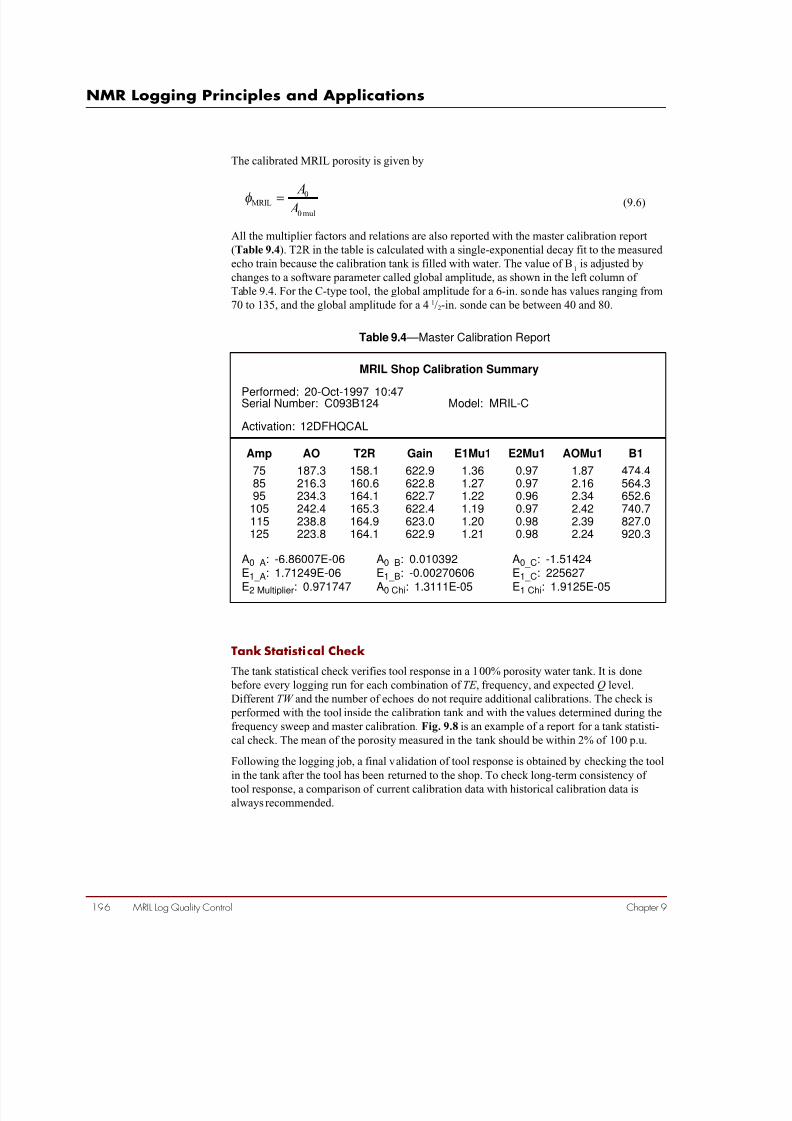
7/28/2019 NMR Logging Principles and Applications
http://slidepdf.com/reader/full/nmr-logging-principles-and-applications 214/253

7/28/2019 NMR Logging Principles and Applications
http://slidepdf.com/reader/full/nmr-logging-principles-and-applications 215/253
MRIL Log Quality Control 197
Halliburton Energy Services
Chapter 9
Figure 9.8 —On the reportof a tank statistical check,the measured porosity
MPHI should be within 2%of 100 p.u. All of the quality
indicators, such as noisefeatures and voltage-
sensor data, should fallwithin their allowableranges.
o m
0 0 1
6 2 8
Results of the calibration and of the tank statistical check are included on the logs and should
be checked against their reference values.
To prepare for an MRIL job, the logging tool is calibrated for each of the basic activations
and for the expected downhole environment.
Electronics Verification
After shop calibration, a primary verification that tool electronics are functioning properly is
performed. In this verification, a field verifier is connected to the tool’s electronics to check
the response of several internal tool parameters. Table 9.5 displays the verification param-
eters and their allowable ranges. The allowable standard deviations for all the noise featuresshould be checked with Table 9.5 and are used as a go/no-go template. Because the

7/28/2019 NMR Logging Principles and Applications
http://slidepdf.com/reader/full/nmr-logging-principles-and-applications 216/253
NMR Logging Principles and Applications
198 MRIL Log Quality Control Chapter 9
Sensor Name
B1
A1NOISE
A1NECH
A1RING
A1OFFSET
GAIN
TEMP1
TEMP2
HVmin
HVmax
15VUP15V
15VN
15VT
15VUM
5VUM
5VA
5VAN
5VD
Normal Range
450750
<12
<12
-3030
-3030
250350
AMBIENT
AMBIENT
530590
570610
192414.815.2
-14.8 -15.2
14.815.2
1924
9.512.5
4.95.1
-4.9 -5.1
4.95.1
Standard Deviation
7.5
2.0
2.0
7.5
2.5
2.5
0.0050.005
0.005
0.005
0.005
0.005
0.005
0.005
0.005
Allowable Tolerance
±25
±2
±2
±2
±2
±15
±10
±10
Table 9.5 —MRIL Field Verification Ranges and Tolerances
verification is only a check of tool electronics, a successful verification alone does notnecessarily ensure correct logging responses. However, if the check fails, the tool should not
be run in the well.
Verifier measurements are repeated at the wellsite before and after logging to yield before-
survey and after-survey verification values. These two sets of values should be compared
with each other, and the before-survey values should also be compared with the primary-
verification values.
In a single verification, A1RING and A1OFFSET , which are RINGING and OFFSET respec-
tively for Frequency 1 in multi-frequency mode, should be approximately equal. A difference
of more than 5 units indicates a problem in either the verifier or the tool electronics.
A1NOISE and A1IENoise, which are the NOISE and IENoise respectively for Frequency 1 in
multi-frequency mode, are dependent on GAIN and will vary from system to system. Their
values should be consistent within each system, and any changes greater than 2 from the
primary verification value to the before-survey value, or from the before-survey value to
after-survey value, may indicate a tool problem.
Table 9.6 is an example of a shop verification report, which shows the measured values
of B1, GAIN , NOISE , IENoise, RINGING , OFFSET , HVmin, HVmax, and temperature of
the transmitter and cartridge, their expected ranges, standard deviations, and
allowable deviations.

7/28/2019 NMR Logging Principles and Applications
http://slidepdf.com/reader/full/nmr-logging-principles-and-applications 217/253
MRIL Log Quality Control 199
Halliburton Energy Services
Chapter 9
B1GAINA1NOISEA1INECHOA1RING
A1OFFSETHVMINHVMAXCart Temp
Tran Temp
Shop301.436342.010
2.7042.5305.106
2.310586.445602.381
32.486
33.047
Expected Range450 - 750250 - 350
<12<12
-30 - 30
-30 - 30530 - 590570 - 610-Ambient
-Ambient
Std. Dev.0.5341.7000.6460.3810.505
0.9670.0000.0000.142
0.261
Allowable Dev7.57.52.02.02.0
2.02.52.5
MRIL Shop Check Summary
Performed: 22-Jun-1998 10:32Serial Number: C179B011 Model: MRIL-C
Statistical Check with Dummy Load Performed: 29-Jun-1998 10:32Activation: cblkbox Experiment Range: 50-150Field Verifier # c107
Table 9.6 —Example of Shop Verification Report Along with Allowed Ranges
Quality Control During Logging
Operating Frequency
The MRIL operating frequency is the center frequency of the B1
field. Before logging, just as
before calibration, a frequency sweep is performed downhole. The transmitter is then set to
operate at the frequency at which the maximum gain was found during the frequency sweep.
MRIL-C tools may be set to operate with two frequencies in dual-frequency mode, both of
which must be selected from one of two frequency ranges: standard frequency (700 to 750
kHz) and low frequency (600 to 650 kHz). The MRIL-Prime tool is set to operate at nine
frequencies: for example, at 760, 686, 674, 656, 644, 626, 614, 596, and 584 kHz. Changing
a tool’s operating-frequency range requires significant hardware modifications that must be
performed at the shop.
Logging Speed and Running Average
MRIL logging speed is affected by many factors. Speed charts, which determine the logging
speed, are based on
• gain • desired vertical resolution
• activation • operating frequency
• polarization time
• tool type (C or Prime)
• tool size

7/28/2019 NMR Logging Principles and Applications
http://slidepdf.com/reader/full/nmr-logging-principles-and-applications 218/253
NMR Logging Principles and Applications
200 MRIL Log Quality Control Chapter 9
Figure 9.9 —This speedchart is designed for use
with a 6-in. MRIL-C tooloperating in dual-fre-quency mode at highfrequency, i.e., 700 to 750
kHz. The upper section ofthe chart is used whenacquiring a high-resolution
log. (A high-resolution logis one having verticalresolution of approximately
4 ft for any gain). Thelower section is used forstandard-resolution logs.(A standard-resolution log
is one having a resolution
of approximately 6 ft forany gain.) Speed chartssuch as the one shown are
available for 6-in. and 4 1 / 2-in. tools; for single-, dual-,and triple-frequencymodes; and for standard-
T 2, dual-TW , dual-TE , andtotal-porosity activations.
6-in.ToolStandard
DualFrequency
For low frequency (600 - 650 kHz) operation:
Increase running average by 50% - round to the nearest multiple of 8.Reduce logging speed by 33%.
TW = 1,500
TW = 3,000
TW = 6,000
TW = 12,000
High Resolution
Logging SpeedRunning Average
High Frequency (700 - 750 kHz) Tools
LoggingSpeed(ft/min)
VerticalResolution(ft)
100
10
10 100 200 300 400 500 600 700
8
16
0
24
32
40
48
56
64
RunningAverage(Mustbemultipleof8)
Dual Frequency Gain
Maximum Logging Speed = 30 ft/min
LoggingSpeed(ft/min)
VerticalResolution(ft)
100
10
10 100 200 300 400 500 600 700
8
16
0
24
32
40
48
56
64
RunningAverage(Mustbemultipleof8)
Dual Frequency Gain
Standard Resolution
TW = 1,500
TW = 3,000
TW = 6,000
TW = 12,000
o m
0 0 1 4 5 4
Information from the speed chart is essential to selecting the correct (minimum) running
average based on tool gain. Fig. 9.9 shows examples of speed charts for the MRIL-C tool. A
different speed chart is designed for each desired vertical resolution, with high-resolution and
standard-resolution charts being shown in Fig. 9.9.
Fig. 9.10 shows of how to use the speed chart in Fig. 9.9. In this example, tool gain is
assumed to be 470, a high-resolution run is desired, and TW is 3000 ms. Beginning at 470 on
the horizontal axis (Dual Frequency Gain), a line is projected vertically until the red Running
Average curve is reached. At this point, a value of 8 is read on the right-side Running
Average scale. When the vertical projection line is continued upward, the green dotted
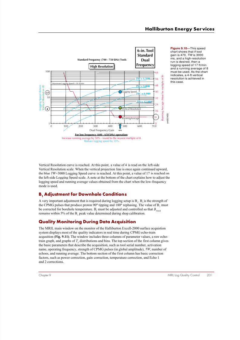
7/28/2019 NMR Logging Principles and Applications
http://slidepdf.com/reader/full/nmr-logging-principles-and-applications 219/253
MRIL Log Quality Control 201
Halliburton Energy Services
Chapter 9
Figure 9.10 —This speedchart shows that if toolgain is 470, TW is 3000
ms, and a high-resolutionrun is desired, then alogging speed of 17 ft/minand a running average of 8
must be used. As the chartindicates, a 4-ft verticalresolution is achieved in
this case.
8
16
0
24
32
40
48
56
64
Ru
nningAverage(Mustbemultipleof8)
LoggingSpeed(ft/min)
VerticalResolution(ft)
100
10
10 100 200 300 400 500 600 700
Dual Frequency Gain
For low frequency (600 - 650 kHz) operation:
Increase running average by 50% - round to the nearest multiple of 8.Reduce logging speed by 33%.
TW = 1,500
TW = 3,000
TW = 6,000
TW = 12,000
High ResolutionHigh Resolution
Standard Frequency (700 - 750 kHz) Tools
470
4
17
Maximum Logging Speed = 30 ft/min
Logging Speed
Vertical Resolution
RunningAverage
6-in.ToolStandard
DualFrequency
o m
0 0
1 4 5 5
Vertical Resolution curve is reached. At this point, a value of 4 is read on the left-side
Vertical Resolution scale. When the vertical projection line is once again continued upward,
the blue TW =3000 Logging Speed curve is reached. At this point, a value of 17 is reached on
the left-side Logging Speed scale. A note at the bottom of the chart explains how to adjust thelogging speed and running average values obtained from the chart when the low-frequency
mode is used.
B1Adjustment for Downhole Conditions
A very important adjustment that is required during logging setup is B1. B
1is the strength of
the CPMG pulses that produce proton 90° tipping and 180° rephasing. The value of B1
must
be corrected for borehole temperature. B1
must be adjusted and controlled so that B1mod
remains within 5% of the B1
peak value determined during shop calibration.
Quality Monitoring During Data Acquisition
The MRIL main window on the monitor of the Halliburton Excell-2000 surface acquistion
system displays most of the quality indicators in real time during CPMG echo-train
acqusition (Fig. 9.11). The window includes three columns of parameter values, a raw echo-train graph, and graphs of T 2
distributions and bins. The top section of the first column gives
the basic parameters that describe the acquisition, such as tool serial number, activation
name, operating frequency, strength of CPMG pulses (in global amplitude), TW , number of
echoes, and running average. The bottom section of the first column has basic correction
factors, such as power correction, gain correction, temperature correction, and Echo 1
and 2 corrections.

7/28/2019 NMR Logging Principles and Applications
http://slidepdf.com/reader/full/nmr-logging-principles-and-applications 220/253
NMR Logging Principles and Applications
202 MRIL Log Quality Control Chapter 9
Figure 9.11 —The MRIL
main window displays mostof the quality indicators so
that the log quality can bemonitored during CPMG
echo-train acquisition.Values shown in this figureare from an echo-train
acquisition in a 100-p.u.water calibration tank.
o m
0 0 1 6 2 9
The top section of the second column displays the measured porosity ( MPHI ), calculated
BVI , and FFI based on a defaut T 2cutoff
, (which is 33 ms for sandstone and 92 ms for carbon-
ates). The bottom section of the second column has the primary quality-control indicators,
such as Chi, gain, B1, B
1mod , and noise features (OFFSET , RINGING , NOISE , and IENoise).
The third column displays auxiliary sensors, such as temperatures (Temp1, Temp2, and
Temp3) from electronic cartridge, transmitter, and magnet, respectively, and all the
electronics voltage-sensor data. When the value of any quality indicator is outside its
allowable range, this window will automatically show a red flash under its name and
warn the field engineer.
Log-Quality Display
All of the quality indicators are recorded in the raw data file and are available for playback
whenever needed. MRIL log quality can be displayed in different ways and formats, one of
which is shown in Fig. 9.12. Track 1 includes gamma ray (GR), cable speed (CS ), and tension
(TENS ). Track 2 contains gains for two groups of echo trains described in the next paragraph
(GAINA and GAINB), amplitudes of the corresponding CPMG pulses ( B1A and B1B), and
amplitudes of corresponding CPMG pulses corrected for temperature ( B1MODA and
B1MODB). Track 3 includes all the voltage sensor data. Track 4 shows the temperatures of
the transmitter (TXTA), electronic cartridge ( ECTA), and antenna ( ANTA). Track 4 also shows
phase-correction parameters, such as the phase angles ( PHCOA and PHCOB), the means of
the imaginary parts of the echo trains ( PHERA and PHERB), standard deviations of theimaginary parts of the echo trains ( PHNOA and PHNOB). Track 5 includes NOISE and
IENoise for Groups A and B and Frequencies 1 and 2 ( N1A, N1B, N2A, N2B, IEN1A,
IEN1B, IEN2A, and IEN2B, where for example, N1A is NOISE for Group A and Frequency
1). Track 6 includes OFFSET and RINGING for Groups A and B and Frequencies 1 and 2.
Track 7 includes Chi for Group A and B, MPHI from Groups A and B, and BVI from
Group A.
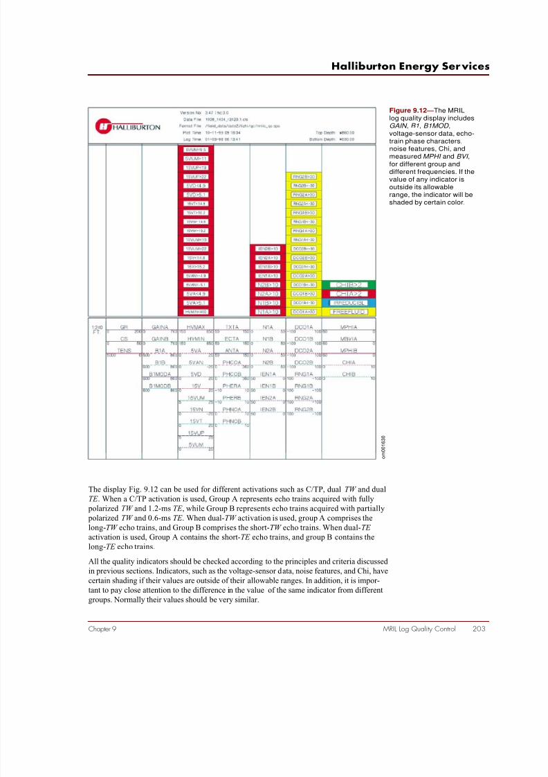
7/28/2019 NMR Logging Principles and Applications
http://slidepdf.com/reader/full/nmr-logging-principles-and-applications 221/253
MRIL Log Quality Control 203
Halliburton Energy Services
Chapter 9
Figure 9.12 —The MRILlog quality display includes
GAIN , B1, B1MOD ,
voltage-sensor data, echo-train phase characters,noise features, Chi, andmeasured MPHI and BVI ,
for different group anddifferent frequencies. If thevalue of any indicator is
outside its allowablerange, the indicator will beshaded by certain color.
o m
0 0 1 6 3 0
The display Fig. 9.12 can be used for different activations such as C/TP, dual TW and dual
TE . When a C/TP activation is used, Group A represents echo trains acquired with fully
polarized TW and 1.2-ms TE , while Group B represents echo trains acquired with partially
polarized TW and 0.6-ms TE . When dual-TW activation is used, group A comprises the
long-TW echo trains, and Group B comprises the short-TW echo trains. When dual-TE
activation is used, Group A contains the short-TE echo trains, and group B contains the
long-TE echo trains.
All the quality indicators should be checked according to the principles and criteria discussed
in previous sections. Indicators, such as the voltage-sensor data, noise features, and Chi, have
certain shading if their values are outside of their allowable ranges. In addition, it is impor-
tant to pay close attention to the difference in the value of the same indicator from different
groups. Normally their values should be very similar.

7/28/2019 NMR Logging Principles and Applications
http://slidepdf.com/reader/full/nmr-logging-principles-and-applications 222/253
NMR Logging Principles and Applications
204 MRIL Log Quality Control Chapter 9
Figure 9.13 —Thisexample of a log-quality
display for dual-TW
logging shows no abnorm-al shading for voltage-
sensor data, noisefeatures, and Chi. All the
indicators for Group A andB and Frequencies 1 and 2
are within their allowableranges. B
1and B
1modvary
with the GAIN changes.
MPHIA, in Track 7, is
greater than MPHIB , whichmeans that a T
1contrast
exists between fluids in thelogged formation. The logquality can be completelyverified if B
1modis checked
with the B 1
found at
calibration and if thelogging speed is verifiedwith the speed chart and
measured gain.
o m
0 0 1 6 3 1
Fig. 9.13 is an example of log quality display for dual-TW logging. Checking the log, no
abnormal shading is present for voltage-sensor data, noise features, and Chi. All the indica-
tors for Groups A and B at Frequencies 1 and 2, are within their allowable ranges. The phase-
correction parameters— PHCOA, PHCOB, PHERA, PHERB, PHNOA, and PHNOB —are
small and stable. B1
and B1mod
vary with the GAIN changes. B1mod
should be further checked
against the shop calibration report and must be within 5% of the peak value of the CPMG
pulse found during calibration. Cable speed is about 6 ft/min. This speed and running average
should be checked with speed chart according to gain, TW , and vertical resolution. Track 7
indicates that a T 1
contrast exists between fluids in the logged formation because MPHIA is
significantly greater than MPHIB.
Raw echo data and T 2
distributions can also be displayed at the well site for quick look and
quality check, as shown in Fig. 9.14. Group data from dual-TW logging are displayed for the
same well and same interval as shown in Fig. 9.13. The tension data is plotted in the depth
track. Tracks 1 and 2 show the bin data for Group A and B, respectively. Tracks 3 and 5
include echo trains from Groups A and B, respectively. Tracks 4 and 6 are T 2
distributions for
Groups A and B, respectively. Tracks 7 and 8 are Chi, gain, MPHI , and MBVI for Group A
and B, respectively. The echo trains can clarify some of noise problems, such as high Chi.

7/28/2019 NMR Logging Principles and Applications
http://slidepdf.com/reader/full/nmr-logging-principles-and-applications 223/253
MRIL Log Quality Control 205
Halliburton Energy Services
Chapter 9
Figure 9.14 —This groupdata, which displays thedual-TW logging for the
same well and sameinterval as shown in Fig.9.10 is available at well sitefor both quick-look and
quality check. The tensiondata is plotted in the depthtrack. Tracks 1 and 2 show
the bin data for Groups Aand B, respectively. Tracks3 and 5 include echo trains
from Groups A and B,respectively. Tracks 4 and 6are T
2distributions for
Groups A and B, respec-
tively. Tracks 7 and 8 areChi, GAIN , MPHI , and
MBVI for Groups A and B,
respectively. Some of the
noise problems, such ashigh Chi, can be clarified bydisplaying the echo trains.
o m
0 0 1 6 3 2

7/28/2019 NMR Logging Principles and Applications
http://slidepdf.com/reader/full/nmr-logging-principles-and-applications 224/253

7/28/2019 NMR Logging Principles and Applications
http://slidepdf.com/reader/full/nmr-logging-principles-and-applications 225/253
MRIL Log Quality Control 207
Halliburton Energy Services
Chapter 9
Agreement between MPHI and Neutron-Density Crossplot Porosity
In clean, water-filled formations, MPHI should be approximately equal XPHI , theneutron-density crossplot porosity. In clean gas zones, MPHI values obtained from
stationary measurements should be near neutron porosity values calculated with the
correct matrix. In shaly sands, MPHI should approximately equal density porosity
calculated with the correct grain density.
Knowledge of the mud type is essential in analyzing the response of an MRIL tool.
Because of the tool’s relatively shallow depth of investigation, the tool investigates
primarily the flushed zone.
Effects of Hydrogen Index and Polarization Time onMPHI
MPHI may not equal effective porosity because of the effects of both hydrogen index
and long T 1
components. The MRIL Prime measurement process usually eliminates the
porosity underestimation that results from the T 1
effects. The measurements are still
affected by HI . In clean gas zones, MPHI values obtained from stationary measurements
should be near neutron porosity values calculated with the correct matrix.
Reference
1. Goelman, G., and Prammer, M.G., 1995, The CMPG pulse sequence in strong
magnetic field gradients with applications to oil-well logging: Journal of Magnetic
Resonance, Series A, v. 113, p. 11-18.

7/28/2019 NMR Logging Principles and Applications
http://slidepdf.com/reader/full/nmr-logging-principles-and-applications 226/253
NMR Logging Principles and Applications
208 MRIL Log Quality Control Chapter 9
7/28/2019 NMR Logging Principles and Applications
http://slidepdf.com/reader/full/nmr-logging-principles-and-applications 227/253
209
Halliburton Energy Services
Glossary
Glossary
A
Activation
Programmed command sequences that control how MRIL tools
polarize formations and measure NMR properties of those formations.
Activations may contain single or multiple CPMG sequences.
Activation, Dual-TE
An activation that enables the acquisition of two CPMG echo trains at
different echo spacings (TE ) but at identical re-polarization times
(TW ). Data acquired with dual-TE activations are used for hydrocarbon
identification. The hydrocarbon identification technique takes advan-
tage of the different diffusivities of the different reservoir fluids.
Because the MRIL tool produces a magnetic field gradient, the T 2
of
each fluid has a component that depends on its diffusivity and on the
TE used in the NMR measurements. Increases in TE will shift the T 2
spectrum toward smaller T 2
values, and the shift will be different for
each fluid type. Separation in T 2
space follows from the diffusion
relaxation term T 2diffusion
12
)( 2TE G D γ
This activation has been successfully used in detecting and quantifying
medium-viscosity oils.
Activation, Dual-TW
An activation that enables the acquisition of two CPMG echo trains at
different wait times (TW ) and identical echo spacings (TE ). Data
acquired with dual-TW activations are used to improve detection of gas
and light oils. This detection is based on the fact that the T 1
of gas and
light oils is much larger than the T 1
of water in a formation. Polariza-
tion p is proportional to TW , i.e.,
11T
-TW
e p −∝
The smaller TW is chosen such that the NMR signal from the formation
water is completely polarized, but the oil and/or gas signals are not.The longer TW is chosen so that most of the hydrocarbon signals are
also polarized. The signal left after the subtraction of the two echo
trains or the two resulting T 2
distributions contains only signal from the
hydrocarbon. This method can be used to quantify oil and gas volumes.
7/28/2019 NMR Logging Principles and Applications
http://slidepdf.com/reader/full/nmr-logging-principles-and-applications 228/253
NMR Logging Principles and Applications
210 Glossary
Activation, Standard-T 2
An activation that enables the acquisition of a CPMG echo train with a TW with
which formation fluids can be fully polarized, and with a TE with which the diffu-
sion effects on T 2
can be eliminated. Typical values for this activation are
TE = 1.2 ms, 3 s ≤ TW ≤ 6 s, and NE = 300. This activation is mainly used for
determining “effective” porosity and permeability.
Activation, Total-Porosity
An activation that enables the acquisition of two CPMG echo trains with different
echo spacings (TE ) and different wait times (TW ). One echo train is acquired with
TE = 0.6 ms and TW = 20 ms (only partial polarization is achieved) and is used for
quantifying the small pores, which are at least in part associated with clay-bound
water. The other echo train is acquired with TE = 0.9 or 1.2 ms and with a TW that
is sufficiently long so that full polarization is achieved. This echo train is used to
determine effective porosity, and the summation of the two porosities (clay-bound
and effective) provides total porosity information. The combination of TE and TW
used to acquire the latter echo train constitutes a standard T 2
activation.
B
B0
Static magnetic field generated by the NMR tool. It may also be designated as Bz.
The symbols B0 and B
z are use when referring to the scalar value of the field.
B1
Oscillating magnetic field generated by a radio-frequency (RF) resonant circuit.
This field is applied in the plane perpendicular to B0
and is used to flip the magnet-
ization by 90° and 180°. B1 refers to the magnitude of the field.
Bound Water
A somewhat loosely defined term that can refer either to water that is not producible
or water that is not displaceable by hydrocarbons. Bound water consists of both
capillary-bound water and clay-bound water.
Bulk Volume Irreducible ( BVI )The fractional part of formation volume occupied by immobile, capillary-
bound water.
Bulk Volume Irreducible, Cutoff (CBVI )
BVI is estimated by summing the MRIL T 2
distribution up to the time T 2cutoff
.
Bulk Volume Irreducible, Spectral ( SBVI )
BVI obtained by the MRIL spectral method. This BVI estimate is determined from a
model that assigns a percent of the porosity in each spectral bin to bound water.
Various models are available for use with this method.
Bulk Volume Movable ( BVM )
The fractional part of formation volume occupied by movable fluids, also referred
to as free fluid index ( FFI ). It can be water, oil, gas, or a combination.
Bulk Volume Water ( BVW )The fractional part of formation volume occupied by water. BVW is the product of
water saturation and total porosity.

7/28/2019 NMR Logging Principles and Applications
http://slidepdf.com/reader/full/nmr-logging-principles-and-applications 229/253
211
Halliburton Energy Services
Glossary
BVI See Bulk Volume Irreducible.
BVM See Bulk Volume Movable.
BVW See Bulk Volume Water .
Bz
see B0
C
Carr-Purcell-Meiboom-Gill Pulse Sequence (CPMG)
A pulse sequence used to measure T 2
relaxation time. The sequence begins with a
90° pulse followed by a series of 180° pulses. The first two pulses are separated by a
time period τ , whereas the remaining pulses are spaced 2τ apart. Echoes occur
halfway between 180° pulses at times 2τ , 4τ , ... , where 2τ equals TE , the echo
spacing. Decay data is collected at these echo times. This pulse sequence
compensates for the effects of magnetic field inhomogeneity and gradients in the
limit of no diffusion, and reduces the accumulation of effectsof imperfections in the 180° pulses as well.
CBVI See Bulk Volume Irreducible, Cutoff .
CBW See Clay-Bound Water .
Clay-Bound Water (CBW )
Immobile structurally bound water on the surface of clay minerals. Clay surfaces
are electrically charged due to ionic substitutions in the clay structure, which allow
them to hold substantial amounts of ionically bound water. This water is referred to
as water of adsorption or surficially bound water. Clay-bound water also includes
water of capillary condensation in the micropores in clay aggregates. CBW is a
function both of the surface area of the clay and the charge density on its surface.
Clay consists of extremely fine particles, so it has a very high surface area. CBW
contributes to the electrical conductivity of the sand but not its hydraulic conduct-
ivity. Clay-bound water cannot be displaced by hydrocarbons and will not flow. Ithas very short T
1and T
2times.
CMR™ Tool*
The Schlumberger Combinable Magnetic Resonance logging tool was
introduced in 1995. The CMR tool is a pad device with a sensitive volume that
extends about 1 in. in front of the pad face. This very shallow depth of investigation
makes the tool very sensitive to invasion, mud cake, and borehole rugosity.
The 6-in. long CMR antenna is placed on the center of a 12-in.long magnet.
This arrangement provides 3 in. of magnet length to polarize protons before they
are measured.
The sensitive volume of the CMR tool is a 1-in. diameter, 6-in. long cylinder. The
CMR tool operates in single-frequency mode.
CPMG See Carr-Purcell-Meiboom-Gill Pulse Sequence.
*Trademark of Schlumberger Technology Corporation
7/28/2019 NMR Logging Principles and Applications
http://slidepdf.com/reader/full/nmr-logging-principles-and-applications 230/253
NMR Logging Principles and Applications
212 Glossary
D
D See Diffusion Constant .
DIFAN See Diffusion Analysis.
Differential Spectrum Method (DSM)
An interpretation method based on dual-TW measurements. DSM relies on the T 1
contrast between water and light hydrocarbon to type and quantify light hydro-
carbons. The differential spectrum is the difference between the two T 2
distributions
(spectra) obtained from dual-TW measurements with identical TE . DSM interpret-
ation is performed in the T 2
domain.
Diffusion
Process by which molecules or other particles intermingle and migrate because of
their random thermal motion.
Diffusion Analysis (DIFAN)
An interpretation method based on dual-TE measurements. DIFAN relies on the
diffusion contrasts between water and medium-viscosity oil to type and quantifyoils. The data for DIFAN are acquired through dual-TE logging with a single, long
polarization time.
Diffusion Constant ( D)
Also known as diffusivity. D is the mean square displacement of molecules ob-
served during a period. D varies with fluid type and temperature. For gas, D also
varies with density and is therefore pressure dependent. D can be measured by
NMR techniques, in particular by acquiring several CPMG echo trains with different
echo spacings in a gradient magnetic field.
Diffusion Limit, Fast
The case where protons carried across a pore by diffusion to the surface layer relax
at the surface layer at a rate limited by the relaxers at the surface and not by the rate
at which the protons arrive at the surface. The diffusion process happens much
faster than that of the fluid protons relaxing in a pore. Thus, the magnetization in the pore remains uniform, and a single T
1or T
2can be used to describe the magnetiz-
ation polarization or decay for an individual pore. This assumption is the basis of the
conversion of T 1
and T 2
distributions to pore-size distributions.
Diffusion Limit, Slow
The case where protons carried across a pore by diffusion to the surface layer relax
at the surface layer at a rate limited not by the relaxers at the surface but by the rate
at which the protons arrive at the surface. Thus, diffusion does not homogenize the
magnetization in the pore space. Multiple exponential decays then are needed to
characterize the relaxation process within a single pore.
Diffusion Relaxation
A relaxation mechanism caused by molecular diffusion in a gradient field during a
CPMG measurement. Molecular diffusion during a CPMG or other spin echo pulse
sequence causes signal attenuation and a decrease in the apparent T 2. This attenu-ation can be quantified and the fluid diffusion coefficient measured if a known
magnetic field gradient is applied during the pulse sequence. Diffusion only affects
the T 2
measurement, not the T 1
measurement.

7/28/2019 NMR Logging Principles and Applications
http://slidepdf.com/reader/full/nmr-logging-principles-and-applications 231/253
213
Halliburton Energy Services
Glossary
Diffusion, Restricted
Effect of geometrical confinement of pore walls on molecular diffusive displace-
ment. NMR diffusion measurements estimate the diffusion constant from the
attenuation caused by molecular motion over a very precise time interval. If the
time interval (TE in the CPMG sequence) is large enough, molecules will encounter
the pore wall or other barrier and become “restricted.” The apparent diffusion
constant will thendecrease.
DSM See Differential Spectrum Method .
E
Echo Spacing (TE )
In a CPMG sequence, the time between 180° pulses. This time is identical to the
time between adjacent echoes.
EDM See Enhanced Diffusion Method .
Enhanced Diffusion Method (EDM)
An interpretation method based on diffusion contrasts between different fluids.
Enhancement of the diffusion effect during echo-data acquisition allows water and
oil to be separated on a T 2
distribution generated from data acquired with a selected
long TE . For typing medium-viscosity oils, EDM uses CPMG measurements
acquired through standard T 2
logging with a long TE . For quantifying fluids, EDM
needs data acquired through dual-TW logging with a long TE or through dual-TE
logging with a long TW .
F
FFI See Free Fluid Index.
FID See Free Induction Decay.Free Fluid Index ( FFI )
The fractional part of formation volume occupied by fluids that are free to flow. A
distinction must be made between fluids that can be displaced by capillary forces,
and fluids that will be produced at a given saturation. In MRIL logging, FFI is the
BVM estimate obtained by summing the T 2
distribution over T 2
values greater than or
equal to T 2cutoff
.
Free Induction Decay (FID)
The FID is the transient NMR signal resulting from the stimulation of the nuclei at
the Larmor frequency, usually after a single RF pulse. The characteristic time
constant for a FID signal decay is called T 2
*. T 2
* is always significantly shorter
than T 2.

7/28/2019 NMR Logging Principles and Applications
http://slidepdf.com/reader/full/nmr-logging-principles-and-applications 232/253
NMR Logging Principles and Applications
214 Glossary
G
G The strength of the gradient magnetic field seen by the NMR measurement.
Gain Represents the relative voltage gain of the system: both the antenna gain and
electronics gain. Because the electronics gain is quite stable, the gain is sensitive to
antenna loading, Q. At the beginning of each pulse sequence, a measured low-level
signal is sent from a test antenna (known as the B1 loop) to the main antenna, and
the received signal is processed just as echoes would be processed. The received
signal is then measured and compared to the original input signal. This provides the
gain. The gain is used to compensate for signal losses due to Q loading effects of
the borehole and due to system drift.
Gauss Unit of magnetic field strength. 10,000 gauss = 1 tesla. The earth’s magnetic field
strength is approximately 0.5 gauss.
Gradient
Amount and direction of the rate of change in space of some quantity, such as
magnetic field strength.Gradient Magnetic Field
A magnetic field whose strength varies with position. The MRIL tool generates a
gradient magnetic field that varies in the radial direction. Within the small sensitive
volume of the MRIL tool, this gradient can be regarded as linear and is usually
expressed in gauss/cm or Hz/mm.
Gyromagnetic Ratio (γ )
Ratio of the magnetic moment to the angular momentum of a particle. A measure of
the strength of the nuclear magnetism. It is a constant for a given type of nucleus.
For the proton, γ = 42.58 MHz/Tesla.
H, I
Hydrogen Index ( HI )
The ratio of the number of hydrogen atoms per unit volume of a material to the
number hydrogen atoms per unit volume of pure water at equal temperature and
pressure. The HI of gas is a function of temperature and pressure.
HI See Hydrogen Index.
Inversion Recovery
A pulse sequence employed to measure T 1
relaxation time. The sequence is “180° - t i
90° -Acquisition - TW ,” where i = 1 … N . The first 180° pulse inverts the magnet-
ization 180° relative to the static magnetic field. After a specific wait time (t i, the
inversion time), a 90° pulse rotates the magnetization into the transverse plane, and
the degree of recovery of the initial magnetization is measured. After a wait time
TW to return to full polarization, the sequence is repeated. To produce sufficient data
for measurement of T 1, this sequence must be repeated many times with different t
i
and thus is very time-consuming.

7/28/2019 NMR Logging Principles and Applications
http://slidepdf.com/reader/full/nmr-logging-principles-and-applications 233/253
215
Halliburton Energy Services
Glossary
L
Larmor Equation
f = γ B0/2π. This equation states that the frequency of precession, f , of the nuclear
magnetic moment in a magnetic field is proportional to the strength of the
magnetic field, B0, and the gyromagnetic ratio, γ .
Larmor Frequency
The frequency at which the nuclear spins precess about the static magnetic field, or
the frequency at which magnetic resonance can be excited. This frequency is
determined from the Larmor equation.
M
M Net magnetization vector. See Magnetization.
M0
Equilibrium value of the net magnetization vector directed along the static
magnetic field.
Magnetization, Longitudinal (Mz)
Component of the net magnetization vector along the static magnetic field
B0
(or Bz).
Magnetic Moment
A measure of the magnetic properties of an object or particle (the proton for
example) that causes the object or particle to align with the static magnetic field.
Magnetic Resonance (MR)
Magnetic resonance describes a group of phenomena more general than NMR. It
also includes nuclear quadruple resonance (NQR) and electron paramagnetic
resonance (EPR). Because the term nuclear is often related with radioactivity, the
term MR is used to avoid this connotation. (NMR means nuclear magnetic reson-ance, i.e., the term nuclear refers to the magnetic resonance of an atomic nucleus.)
Magnetic Resonance Image Logging (MRIL)
The name for the specific NMR logging tool developed by NUMAR Corporation in
the mid-1980s. The MRIL tool uses a permanent gradient magnetic field and an
orthogonal RF magnetic field (for generating CPMG pulse sequences) to select
concentric cylindrical shell volumes for NMR measurements.
Magnetic Resonance Imaging (MRI)
Refers to imaging with NMR techniques. Most MRI machines use a pulsed gradient
magnetic field that permits one to localize the NMR signals in space. MRI is used
on core samples and in core flooding or flow mechanism studies.
Magnetic Susceptibility (χ)
The measure of the ability of a substance to become magnetized. Differences
in magnetic susceptibility of the pore fluids and the matrix cause internalfield gradients.
Magnetization (M)
A macroscopic vector quantity resulting from the alignment of the nuclear magnetic
moment with the static magnetic field. This vector projected into the plane perpen-

7/28/2019 NMR Logging Principles and Applications
http://slidepdf.com/reader/full/nmr-logging-principles-and-applications 234/253
NMR Logging Principles and Applications
216 Glossary
perpendicular to the static magnetic field is known as the transverse magnetization.
It is this quantity that is observed by NMR.
MAP A software program developed by NUMAR for inverting echo-train data to a T 2distribution. The inversion algorithm used in MAP is based on singular-value
decomposition (SVD).
MCBW CBW estimate obtained by summing the T 2
distribution obtained from partially
polarized CPMG echo trains acquired with a TE = 0.6 ms and TW = 20 ms.
MPERM
Permeability estimate obtained from MRIL measurements. Many formulas are in use
for determining permeability from NMR measurements. The two most commonly
used are the Coates equation and the Schlumberger-Doll Research (SDR) equa-
tion. According to the Coates equation,
24
=
BVI
FFI
C k
φ
where C is an empirically determined constant.
According to the SDR equation,
gmT ak 2
2
4φ =
where T 2 gm
is the geometric mean of the T 2
distribution, a is constant, and φ
is porosity.
MPHI The porosity estimate obtained by summing the T 2
distribution over T 2
values
greater than or equal to 4 ms and less than or equal to the highest T 2
value in the
distribution, e.g., 1024 ms. MPHI is often referred to as the effective porosity.
MR See Magnetic Resonance.
MRI See Magnetic Resonance Imaging .
MRIAN
See MRIL Analysis.
MRIL See Magnetic Resonance Imaging Logging.
MRIL Analysis (MRIAN)
An interpretation method that incorporates deep resistivity data, MRIL standard T 2
logging measurements, and the dual water model. MRIAN determines water-filled
porosity in the virgin zone, which can be compared with the flushed-zone results
provided by MRIL stand-alone analysis techniques, such as TDA, EDM,
and DIFAN.
MRIL B0 Radial DependenceThe static magnetic field B
0of the MRIL tool is a gradient field, whose strength B
0
decreases as the distance from the tool axis increases. The radial dependence is
B0 ∝r -2, where r is the distance from the axis of the tool.
7/28/2019 NMR Logging Principles and Applications
http://slidepdf.com/reader/full/nmr-logging-principles-and-applications 235/253
217
Halliburton Energy Services
Glossary
MRIL B0
Temperature Dependence
The static magnetic field B0
of the MRIL tool is generated by a permanent magnet.
The temperature dependence of the strength of B0
arises from the fact that the
magnetization of the permanent magnet is temperature dependent. The mean
field approximation gives T -1 temperature dependence in the temperature regime,
typical of borehole conditions, where T is the absolute temperature.
MRIL B1
Temperature Correction
The B1
90° pulse is determined during the MRIL shop calibration done at room
temperature. Because of the difference between room temperature and downhole
temperature, the energy of the B1 pulse needed for 90° tipping downhole will be
different from the energy determined at the shop; therefore, a temperature correction
for B1
is needed.
MRIL Borehole Washout Effect
An MRIL log will show the effect of serious borehole washouts when the sensitive
volume intersects the borehole. An increase in MPHI and BVI will be seen in the log
response. The MRIL tool responds to water-based mud as bound formation fluid
because of the large quantity of dispersed clays and the associated water of hydration. Oil-based mud exhibits short relaxation times because of the large quan-
tities of emulsifiers used to control water.
Washouts may be affecting an MRIL log if
• A comparison of caliper measurements with the depth of investigation for the
appropriate downhole temperature indicates that the borehole is intersecting the
sensitive volume of the tool.
• An abnormally large BVI is observed.
• An increase in MPHI corresponds to an increase in the caliper and
MBVI = MPHI .
MRIL-C Tool
NUMAR’s second-generation MRIL tool introduced in 1994. This tool is capable of performing multiple experiments simultaneously (e.g., the MRIL-C has dual-
frequency capability, and the MRIL-C+ has triple-frequency capability). The
MRIL-C/TP tool, which was introduced by NUMAR in 1996, provides an estimate
of total porosity as well as effective porosity. The C/TP tool is able to measure total
porosity because the tool can use a reduced TE (0.6 ms). Furthermore, because
the tool experiences reduced ringing, the first echo contains valuable information.
Because MRIL-C tools operate in either dual- or triple-frequency mode, successive
measurements at different frequencies can follow one another more quickly. Each
MRIL frequency excites a signal from a different physical locations and thus it is not
necessary to wait for repolarization to occur in one location before making a mea-
surement in another location. Alternating between frequencies allows more
measurements to be made in a given time, thus permitting logging speed to be
increased without reducing S/N , or permitting S/N to be increased without reducing
logging speed.
MRIL Depth of Investigation
The depth at which the MRIL tool provides information about. Because the Larmor
frequency is a function of B0
and B0is radially dependent, the Larmor frequency is
7/28/2019 NMR Logging Principles and Applications
http://slidepdf.com/reader/full/nmr-logging-principles-and-applications 236/253
NMR Logging Principles and Applications
218 Glossary
also radially dependent and thus defines the depth of investigation of the MRIL
tool. Furthermore, because B0
is also temperature-dependent, it follows that the
Larmor frequency and thus the depth of investigation are also temperature-depen-
dent when a fixed B1
frequency is used, which is always the case. As the temperature
of the magnet increases, B0
decreases, and the depth of investigation decreases
accordingly (e.g., a depth of investigation of about 16 in. at 25ºC decreases to about
14 in. at 150ºC). The variation of depth of investigation with temperature for MRIL
tools is discussed and displayed in NUMAR literature and charts.
MRIL-Prime Tool
NUMAR’s latest generation of MRIL tool introduced in 1998. This tool is capable
of performing multiple experiments at up to nine frequencies. By alternating
between nine frequencies, measurements can be made at a much higher rate.
The MRIL-Prime provides measurements of clay-bound water, effective porosity,
capillary-bound water, and hydrocarbon typing in just one pass. Besides saving time,
acquiring all the data in one pass eliminates depth-shift errors.
The MRIL-Prime tool has additional pre-polarization magnets placed above and
below the antenna that allow for full polarization of the fluids. This pre-polarizationdesign can provide 12 s of polarization at logging speeds as high as 24 ft/min.
Furthermore, the capability of the tool to fully polarize fluids at high logging speeds
and obtain a full T 2
distribution without any corrections makes the logging results
much less sensitive to certain job-design parameters. Planning logging jobs for
earlier tools required some knowledge of the time needed to polarize fluids. The
MRIL-Prime tool can simply handle the longest polarization times without reducing
logging speed. Thus, this tool can be run much like standard triple-combo tools—
just run the tool to the bottom of the hole and log up without special passes in the
hole and without having to subsequently assemble data from different passes. This
is why the MRIL-Prime tool is the first NMR device that can realistically be con-
sidered a “primary formation evaluation” logging tool.
MRIL Sensitive-Volume Thickness
The thickness of the zone for which the MRIL tool provides information. Thethickness of the sensitive volume for the MRIL tool is approximately 1 mm and
is a function of the gradient strength of the B0
field and the frequency band of
the B1
field.
MSIG Porosity estimate obtained by combining data from dual-TE logging with TE = 0.6
and 1.2 ms. MSIG should agree well with total porosity measured on cores. MSIG =
MCBW + MPHI .
Mud Doping
The practice of adding magnetite to the drilling mud. With the now obsolete NML
tool, doping was essential to kill the borehole signal. However, doping the mud with
a paramagnetic substance to change the NMR properties of invading mud filtrate
may still be desirable. For instance, if the invaded zone is flushed with paramagnetic
ions, then the bulk relaxation time of the brine is shortened, and water signals are
killed. Thus, only oil signals remain, and residual oil saturation can be determined
through NMR measurements. MnCl2, has recently been shown to be a cost-effective
doping agent for this application.
Mx
See Transverse Magnetization.
Mz
See Longitudinal Magnetization.

7/28/2019 NMR Logging Principles and Applications
http://slidepdf.com/reader/full/nmr-logging-principles-and-applications 237/253
219
Halliburton Energy Services
Glossary
N
N E Number of echoes in a CPMG echo train.
NML ™ Tool*
The Nuclear Magnetic Logging tool, an obsolete NMR logging tool that utilized the
earth’s magnetic field. The NML tool measured the precession of hydrogen protons
in the earth’s magnetic field after the alignment of protons with a superimposed
magnetic field. The sensitive volume of the NML was not a thin cylindrical shell, but
a full cylinder centered around the tool; therefore, the measurement contained
borehole signals. Operation of the NML required special doping of the borehole
fluids to eliminate the signal from the protons in the borehole.
NMR See Nuclear Magnetic Resonance.
Nuclear Magnetic Resonance (NMR)
NMR, as a physical phenomenon, is the absorption or emission of electromagnetic
energy by nuclei in a static magnetic field, after excitation by a stable RF magnetic
field. NMR, as an investigative tool, is a method that uses the NMR phenomenon toobserve the static and dynamic aspects of nuclear magnetism. The method requires
a static magnetic field to orient nuclear magnetic moments, and an orthogonal
oscillating field (at RF frequencies) to excite the nuclear magnetic moments. The
frequency of the oscillating field must satisfy the Larmor resonance condition.
NMR can be used to detect molecular structures and probe molecular interactions.
It is a major chemical spectroscopic technique with many applications, including
probing properties of fluids in porous media.
Despite the term nuclear , NMR does not involve radioactivity.
P
PAP See Phase Alternate Pairs.
Paramagnetic Materials
Materials with a small but positive magnetic susceptibility. The addition of a small
amount of paramagnetic material to a substance may greatly reduce the relaxation
times of the substance. Most paramagnetic substances possess an unpaired electron
and include atoms or ions of transition elements (e.g., manganese and vanadium) or
rare earth elements. Oxygen (O2) is also paramagnetic and contributes to the
relaxation of water. Paramagnetic substances are used as contrast agents in medical
MR imaging and to dope the borehole fluids in some applications of NMR logging.
Copper sulfate (CuSO4) is used to dope the water in a calibration tank to reduce
water relaxation times, thereby significantly reducing MRIL calibration time.
Permeability, Absolute
A measure of the ability of a rock to conduct a fluid or gas through its intercon-
nected pores when the pores are 100% saturated with that fluid. Measured in darcies
or millidarcies (md).
Permeability, Effective
The capability of a rock to conduct a fluid in the presence of another fluid, immis-
cible with the first, is called its effective permeability to that fluid. Effective perm-
*Trademark of Schlumberger Technology Corporation.
7/28/2019 NMR Logging Principles and Applications
http://slidepdf.com/reader/full/nmr-logging-principles-and-applications 238/253
NMR Logging Principles and Applications
220 Glossary
permeability not only depends on the permeability of the rock itself, but also on the
relative amounts of the different fluids in the pores.
Permeability, RelativeThe ratio between the effective permeability to a given fluid at a partial saturation
and the permeability at 100% saturation. Relative permeability is the ratio of the
amount of a specific fluid that will flow at a given saturation, in the presence of
other fluids, to the amount that would flow at a saturation of 100%, other factors
remaining the same.
Phase Alternate Pairs (PAP)
A method of acquiring two echo trains that are 180° out of phase. The change in
echo-train phase is accomplished by changing the phase of the initial 90° pulse in
the CPMG sequence by 180°. The effect of this change is to reverse the sign of the
echo data. In processing, the two echo trains are subtracted to eliminate the effects
of ringing and baseline offset.
Polarization Time (TW )
See Wait Time.
Pore-Size Distribution (From T 2
Distribution)
A rock generally consists of a large number of pores of different sizes. Neglecting
interpore fluid exchange, relaxation in a rock saturated with a single-phase fluid can
be viewed as relaxation of a collection of isolated pores of different sizes. The
relaxation distribution is a superposition of the relaxation rates of the individual
pores. In the fast diffusion limit, the T 2
of a fluid in a single pore is determined by
BT V
S
T 2
2
2
11+= ρ
Where T2B
is the bulk fluid relaxation rate. For smaller pores as found in most
sandstones,V
S
T B2
2
1ρ << and can be ignored.
When two or three fluid phases are present, however, the non-wetting phases
occupy the larger pores while the wetting phase occupies the smaller pores because
of the capillary effect. In addition, the relaxation rate of non-wetting fluids is
smaller than that of wetting fluids because the T 2
of non-wetting fluid does not
include the surface term. Both the capillary and surface effect result in shorter T 2
for
wetting-phase fluids compared to the T 2
for the same fluid types in bulk. Much less
change is expected for the non-wetting fluid T 2. Thus, different fluid phases can be
identified by carefully analyzing the T 2
distribution or by using relaxation-weighting
techniques (such as dual TW and dual TE ) for multiphase saturation cases.
Porosity, Effective
A somewhat arbitrary term sometimes used to refer to the fractional part of form-
ation volume occupied by connected porosity and excluding the volume of water associated with clay. In NMR logging, the term has usually been associated with
porosity that decays with T 2
greater than 4 ms.

7/28/2019 NMR Logging Principles and Applications
http://slidepdf.com/reader/full/nmr-logging-principles-and-applications 239/253
221
Halliburton Energy Services
Glossary
Effective porosity often refers to the interconnected pore volume occupied by
movable fluids, excluding isolated pores and pore volume occupied by adsorbed
water. Effective porosity contains fluid that may be immovable at a given saturation
or capillary pressure. For shaly sands, effective porosity is the fractional volume of a
formation occupied by only fluids that are not clay bound and whose hydrogen
indexes are 1.
Porosity, Total
The total pore volume occupied by fluids in a rock. Includes isolated non-connected
pores and volume occupied by adsorbed, immobile fluids. For a shaly sand form-
ation, total porosity is the fractional part of formation volume occupied by both
clay-bound and non-clay-bound fluids.
Precession
The motion of the axis of a spinning body so as to trace out a cone. It is caused
by the application of a torque tending to change the direction of the rotation axis.
The precession of the proton spin axis about the B0
field axis occurs at the
Larmor frequency.
Proton
A positively charged elementary particle that provides the charge in an atomic
nucleus. A hydrogen nucleus contains one proton. The symbol 1H is used to
designate the hydrogen nucleus.
Proton Density
The concentration of mobile hydrogen atoms per unit volume. NMR data can be
corrected for hydrogen density changes by dividing the apparent NMR porosity by
the appropriate hydrogen index.
Pulse, Hard
A term used to describe a high-power, short-duration RF pulse used in NMR pulse
sequences. In contrast, soft pulses are usually low-power, long-duration RF pulses.
Hard pulses are usually rectangular shaped in the time domain and excite wide
frequency bands often extending beyond the desired resonance frequency. Hard pulses generally make good use of available RF power but exhibit poor frequency
selectivity. Because of the narrower pulse widths, hard pulses are more suitable for
pulse sequences that require short echo spacing (TE ). See Pulse Shaping for
frequency selectivity.
Pulse Shaping
The amplitude, shape, and width of RF pulses define the frequency selectivity of an
NMR measurement (see also Hard Pulse and Soft Pulse). Soft pulses are shaped to
improve their frequency selectivity as well as other parameters. How shaping brings
about these improvements can be easily understood by taking the Fourier transform
of RF pulses. A hard pulse is rectangular in shape and excites a wide range of
frequencies far from the main lobe. Thus, the frequency selectivity of a hard pulse
is poor. A soft pulse has a greater spread in the time domain, but excites a narrow,
uniform range of frequencies. Thus, the frequency selectivity of a soft pulse is good.
Pulse, Soft
Low-power, long-duration RF pulses used in NMR measurements. Soft pulses in
time domain are rectangular pulses in frequency domain. In medical MRI applica-
tions, a soft 90° pulse typically has a width of a few milliseconds. Although soft
pulses need not conform to a particular shape, they usually have crafted pulse
7/28/2019 NMR Logging Principles and Applications
http://slidepdf.com/reader/full/nmr-logging-principles-and-applications 240/253
NMR Logging Principles and Applications
222 Glossary
envelopes, e.g., truncated Sinc pulses (bell-shaped envelopes), to improve frequency
selectivity. See Pulse Shaping for frequency selectivity.
Pulse, 90°An RF pulse designed to rotate the net magnetization vector 90° from its initial
direction in the rotating frame of reference. If the spins are initially aligned with the
static magnetic field, this pulse produces transverse magnetization and free
induction decay (FID).
Pulse, 180°An RF pulse designed to rotate the net magnetization vector 180° in the rotating
frame of reference. Ideally, the amplitude of a 180° pulse multiplied by its duration
is twice the amplitude of a 90° pulse multiplied by its duration. Each 180° pulse in
the CPMG sequence creates an echo.
R
Radio Frequency (RF)Electromagnetic radiation at a frequency in the same general range as that used for
radio transmissions.The Larmor frequency for 1H is typically in this range. For an
MRIL tool, the Larmor frequency is in the range of 580 to 750 KHz.
Regularization
The process which is used to stabilize the inversion from the measured NMR echo
decay to the T 2
spectra. There are many methods in use, of which MAP is one. They
all result in a smoothed spectra, which varies depending on the method and amount
of regularization. The need to use regularization means that there is no unique NMR
spectra or pore distribution. In most cases, the major features of the spectra are
independent of the method of regularization.
Relaxation Time
A time constant associated with the return of nuclear spins to their equilibrium
positions after excitation. Several relaxation times are defined in NMR measure-ments. Each is related to different molecular interaction mechanisms. The most
frequently measured relaxation times are T 1
and T 2. For bulk water, T
1and T
2are
approximately 3 s. The relaxation times of water in rocks are much smaller and are
generally less than 300 ms.
Relaxation Time, Bulk Fluid
The relaxation produced by interaction of the fluid with itself. For most cases of
interest T 1
and T 2
are equal. For gas, however, because the diffusivity of gas is much
higher than that of liquids, the apparent T 2
of gas measured by CPMG technique in a
gradient magnetic field can be much smaller than T 1.
Relaxation Time, Longitudinal (T 1)
Longitudinal, or spin-lattice, relaxation time. This time constant characterizes the
alignment of spins with the external static magnetic field.
Relaxation Time, Transverse (T 2)
Transverse, or spin-spin, relaxation time. This time constant characterizes the loss of
phase coherence that occurs among spins oriented at an angle to the main magnetic
field and that is due to interactions between spins. T 2
never exceeds T 1. Both T
2and

7/28/2019 NMR Logging Principles and Applications
http://slidepdf.com/reader/full/nmr-logging-principles-and-applications 241/253
223
Halliburton Energy Services
Glossary
T 1
have been successfully related to petrophysical properties of interest, such as
pore size, surface-to-volume ratio, formation permeability, and capillary pressure.
Residual OilOil remaining in the reservoir rock after the flushing or invasion process, or at the
end of a specific recovery process or escape process.
Resonance
Vibration in a mechanical or electrical system caused by a periodic stimulus, with
the stimulus having a frequency at or close to a natural frequency of the system.
RF See Radio Frequency.
Ringing
The oscillatory response of a magnet to the application of high-energy RF pulses.
When the MRIL RF antenna is energized with high-energy RF pulses, the MRIL
magnet resonates or “rings.” The MRIL magnet acts like a piezoelectric crystal,
generating an acoustic oscillating voltage that interferes with the formation signal.
Ringing is frequency-dependent, and each magnet has a different ringing window
(typically 20 to 40 kHz wide) where the ringing effect is smaller than at other
frequencies. The ideal operating frequency is one that is located in the middle of a
broad ringing window.
Rotating Frame of Reference
A frame of reference, which rotates around the axis of the static magnetic field (B0)
at a frequency equal to that of the applied RF magnetic field (B1).
Running Average
This represents the total number of individual experiments (i.e., complete echo
trains) needed to produce a high signal-to-noise. Because the PAPs technique is
used during a CPMG measurement, the Running Averaging is at least two.
S
SBVI See Spectral Bulk Volume Irreducible.
Shifted Spectrum Method (SSM)
An interpretation method based on dual-TE measurements with identical TW . The
SSM relies on the diffusivity contrast between fluids with different diffusivity to
type viscous hydrocarbons. The shifted spectrum refers to the observation of the T 2
distribution shifted to smaller T 2
values when TE is increased. Gases have much
higher diffusivity than oil or water, and are more sensitive to the echo spacing (TE )
changes. Heavy oils have very low diffusivity, and are least sensitive to TE changes.
The SSM is performed in the T 2
domain and uses the difference in the shift between
fluids of different diffusivity to identify fluids.
Signal Averaging
A method of improving signal-to-noise ratio by averaging echo trains.
Signal-to-Noise Ratio ( S/N )
The ratio of signal amplitude to noise amplitude. Signal refers to the desired part of
a detected signal; noise refers to the remainder of the detected signal and includes
random noise. S/N is a measure of data quality. The S/N of NMR measurements can

7/28/2019 NMR Logging Principles and Applications
http://slidepdf.com/reader/full/nmr-logging-principles-and-applications 242/253
NMR Logging Principles and Applications
224 Glossary
be improved by averaging several echo trains, by sampling larger volumes, or by
increasing the strength of the B0
magnetic field. If the noise is random (statistical)
noise only, then averaging n measurements improves S/N by n1/2.
S/N See Signal-to-Noise Ratio.
Spin Intrinsic angular momentum of an elementary particle or system of particles, such
as a nucleus. Spin is responsible for the magnetic moment of the particle or system.
Spin Echo
After spins are excited by an RF pulse, the spins experience FID because of B0
inhomogeneities. Spin isochromats, which are groups of spins precessing at exactly
the same Larmor frequency, lose phase coherence during FID. However, during this
decay, the isochromats do not experience many spin-spin interactions and still retain
phase memory. If a second pulse (180º) is applied at time τ after the first RF pulse,
the spin isochromats will re-phase in the same amount of time τ . A macroscopic
signal (the spin echo) then occurs at precisely TE = 2τ . Even if the second pulse is
not a 180º pulse, a spin echo can still be observed, but this echo will be of smaller
amplitude. A third pulse will repeat the process.
Stimulated Echo
The echo formed after magnetization evolves first in the x-y plane, then in the z
direction, and again in the x- y plane. A stimulated echo is observed after a three-
pulse sequence. Because of B1
inhomogeneities, stimulated echoes occur during
CPMG sequences used on logging tools at the same times as regular echoes and
must be compensated for through calibration.
Surface Relaxivity ( ρ ρ ρ ρ ρ)
A measure of the capability of a surface to cause protons to relax, i.e., lose orient-
ation or phase coherence. This quantity depends on the strength of fluid-matrix
interactions. It also varies with the wettability of the rock surface. Surface relaxation
strength ρ falls in the range of approximately 0.003 to 0.03 cm/s for clastics. ρ is
smaller for carbonates.
T
T 1
See Longitudinal Relaxation Time.
T 2
See Transverse Relaxation Time.
T 2* Time constant characterizing the loss of phase coherence that occurs among spins
oriented at an angle to the main magnetic field and that is due to a combination of
magnetic field inhomogeneity and magnetic interaction. T 2* is always much shorter
than T 2. In the limit of no diffusion, loss of coherence produced by field inhomo-
geneity can be reversed by the application of 180º pulses, which results in the form-
ation of spin echoes.
T 2cutoff
A value of T 2
that is empirically related to the capillary properties of the wetting
fluid in a rock. It is used to differentiate different pore sizes and quantify theamount of bound water. Typically, porosity associated with T
2values less than
approximately 33 milliseconds (T 2cutoff
= 33 ms) are summed to obtain BVI for

7/28/2019 NMR Logging Principles and Applications
http://slidepdf.com/reader/full/nmr-logging-principles-and-applications 243/253
225
Halliburton Energy Services
Glossary
clastics and, similarly, T 2cutoff
of approximately 90 ms for carbonates. Note that these
values are empirical and may be rock-specific.
T 2S Time constant that describes the contribution of surface relaxivity to the transverserelaxation time of fluid in a rock. When a single wetting fluid fills the pores, T
2S
dominates the relaxation process. Thus, T 2
is proportional to (S/V )-1 of a pore, where
S/V is the surface-to-volume ratio. If a spherical pore is assumed, T 2
is proportional
to the pore radius.
TDA See Time Domain Analysis.
TE See Echo Spacing .
Time Domain Analysis (TDA)
An alternate method to the differential spectrum method for processing dual-TW
echo trains. The interpretation is performed in the time domain rather than in the T 2
domain. The key features of the TDA are subtraction of the two echo trains from one
another, and the processing of the echo differences in the time domain using pre-
dicted or measured oil, gas, and water relaxation times and hydrogen-index values.
In the DSM, the dual-TW echo trains are first inverted into T 2
spectra and subtracted
from one another. The interpretation is done in T 2
spectrum domain. The effect of T 2
spectrum broadening because of noise and regularization smears the partial porosi-
ties into adjacent bins, and the subtracted spectrum may contain negative amplitudes
that are obviously incorrect. The TDA method has fewer problems with the noise-
induced T 2spectrum broadening, and because fewer free parameters need to be
determined, the solution is more stable. However, subtracting echoes reduces S/N .
Transverse Magnetization (Mx)
Component of the net magnetization vector at right angles to the static
magnetic field.
TW See Wait Time.
V, W
Viscosity
Resistance of a fluid to flow. Viscosity is due to internal friction caused by
molecular cohesion in the fluid. The diffusion constant D is inversely proportional
to viscosity.
Wait Time (TW )
The time between the last CPMG 180° pulse and the first CPMG pulse of the next
experiment at the same frequency. This time is the time during which magnetic
polarization or T 1
recovery takes place. It is also known as polarization time.
Water-Wet
A solid surface is water-wet when the adhesive attraction of water molecules for the
solid substance is greater than the attraction between water molecules, i.e., adhesive
force > cohesive force. The angle of contact of a water droplet on a water-wet solid
surface will be less than 90° (measured inside the water phase). A mobile non-
wetting oil phase would advance over the adhesive layer of water. Only water has
a surface relaxation mechanism in a water-wet formation.

7/28/2019 NMR Logging Principles and Applications
http://slidepdf.com/reader/full/nmr-logging-principles-and-applications 244/253
NMR Logging Principles and Applications
226 Glossary
Wettability
The capability of a solid surface to be wetted when in contact with a liquid. A liquid
wets a solid surface when the surface tension of the liquid is reduced so that the
liquid spreads over the surface. Only the wetting fluid in a rock pore has a surface
relaxation mechanism. Therefore, wettability affects the NMR properties of fluids in
reservoir rocks.
Nomenclature
γ See Gyromagnetic Ratio.
ρ See Surface Relaxivity.
χ See Magnetic Susceptibility.
η See Viscosity
φ Porosity
References
Glossary of Magnetic Resonance Imaging Terms, in Bushong, S.C., Magnetic Resonance
Imaging, Physical and Biological Principles, Second Edition, Mosby, 1996.
Glossary of Terms and Expressions Used in Well Logging , Second Edition, SPWLA,
Houston, 1984.
NMR Terminology Glossary, Western Atlas, 1996.

7/28/2019 NMR Logging Principles and Applications
http://slidepdf.com/reader/full/nmr-logging-principles-and-applications 245/253
22
Halliburton Energy Service
Index
Index
A
A0, 193
A0mul
, 194A1IENoise , 198A1NOISE , 198
A1OFFSET , 198A1RING , 198
accelerated pre-polarization, 106activation, 4, 104, 114, 199
dual-TE , 104, 123, 167, 174, 175, 176dual-TW , 104, 114, 167, 172partial-polarization, 106
standard, 166, 168standard T
2 , 104, 166, 168, 188
total-porosity, 25, 104, 148, 188activation set, 166
advanced activations, 166ambient signal, 187
ANTA, 202
antenna, 93, 94RF, 185
antenna coil, 102apparent diffusion coefficient (D
a ), 122
apparent porosity, 164, 165, 170apparent water conductivity (C
wa ), 137
Archie’s Law, 64Argentina, 147Australia, 16
B
B0, 34, 96
B1, 93, 96, 186, 193, 194, 199, 201, 202, 204
B1 coil, 185B1A, 202B1B, 202
B 1mod
, 186, 201, 202, 204bin-distribution plot, 8black oil, 178
borehole fluid resistivity, 185borehole rugosity, 26
bound fluids, 11bound water, 45
bulk fluid processes, 46bulk fluid relaxation, 78
bulk longitudinal relaxation time (T 1), 160
bulk volume irreducible (BVI ), 9, 25bulk volume of irreducible water, 57
BVI , 9, 16, 25, 55, 57, 60, 64, 66, 96, 124, 142, 202
C
cable speed (CS ), 202calibration, 185
capacitor voltage, 188capacitors, 108, 188
capillary pressure, 9,16, 59capillary pressure curves, 57, 64capillary-bound water, 4, 11, 25, 65, 121, 142, 148
carbonates, 55, 177, 181Carr, 40
Carr, Purcell, Meiboom, and Gill, 40
CBVI , 64CBVWE , 139C cw
, 136cementation exponent, 136
centralizers, 108centrifuge, 58
centrifuging, 9chalk, 60, 80, 181
Chi (χ), 186, 202clay, 7, 66
clay-bound water (MCBW ), 4, 7, 11, 25, 65, 66, 101,135, 139, 140, 142, 148, 152
clay-bound water porosity (MCBW ), 135
clay-bound-water saturation, 136coarsening-upward sequence, 25
Coates, 64Coates equation, 150
Coates model, 9, 142completion programs, 152conductivity of clay-bound water, 136
conductivity of formation water, 136

7/28/2019 NMR Logging Principles and Applications
http://slidepdf.com/reader/full/nmr-logging-principles-and-applications 246/253
NMR Logging Principles and Applications
228 Index
core porosity, 16Cotton Valley, 152CPMG, 33, 40, 42, 46, 48, 50, 51, 94, 98, 104
crude oil, 78, 85, 163
CS , 202cumulative porosity, 159Curie’s Law, 35
C wa
, 137cycle time (TC), 95
D
D , 5, 6, 49, 82, 83, 84
D a, 122
D g , 49
D o , 49, 163
D w , 49
D 0, 159, 160
dead oil, 47, 77deep resistivity, 135, 147
density/neutron crossplot, 140dephase, 39dephasing, 39, 93
depth of Investigation, 5, 25, 91, 93, 96, 135, 146D
g, 162
D gas
, 82diameter of investigation, 26
diatomite, 181DIFAN, 113, 124, 127, 167differential echo analysis, 180
differential signal, 170differential spectrum, 85, 121, 180
Differential Spectrum Method (DSM), 113Differential Spectrum/Time Domain Analysis, 104
diffusion, 11, 26, 40, 46, 48, 50, 78, 85, 163apparent diffusion coefficient D
a , 122
Diffusion Analysis (DIFAN), 113, 122, 167
diffusion coefficient, 78, 124diffusion contrast, 85, 127, 149
diffusion phenomenon, 124diffusion relaxation, 127
diffusion-induced relaxation, 48enhanced diffusion method (EDM), 13, 127,
129, 147, 148, 149, 150, 167fast diffusion limit, 48quantitative diffusion analysis (DIFAN), 124
shifted spectrum/diffusion analysis, 104T
2diffusion, 46, 48, 82, 87
T 2diffusion,w
, 129unrestricted diffusion, 160
diffusivity (D ), 5, 6, 11, 176
diffusivity contrast, 174distribution, 7, 201
D oil
, 82D
0,mf ,
DSM, 16, 113, 116, 167
dual TE , 26, 78, 82, 83, 85, 104,106, 123, 140, 150,
177, 188dual-TE activation, 104, 123, 167, 174, 175, 176dual-TE logging, 123, 124, 206
dualTW , 25, 78, 80, 84, 88, 89, 104, 106, 113, 114,121, 140, 148, 169, 188
dual-TW activation, 104, 114, 167, 172
dual-TW logging, 116, 142, 204dual-water model, 4, 135, 136
dummy load, 193D w , 82
E
E 1mul
, 194
E 2mul, 194E
amp(i), 189
East Texas, 152echo signal, 2echo spacing (TE ), 106
inter-echo spacing (TE ), 6long echo spacing (TE
L), 123
short echo spacing (TE S ), 123
echo-fit, 53
EDM, 113, 127, 129, 147, 148, 149, 150, 167effective porosity, 4, 7, 139, 148effective relaxivity, 55
energy-storage cartridges (capacitors), 108enhanced diffusion method (EDM), 13, 127, 129,
147, 148, 149, 150, 167E x (i), 189
exploration areas, 177E y (i), 189
F
fast diffusion limit, 48FFI , 58, 202
FID, 39fining downward, 142
fluid properties, 45, 159, 161
fluid saturation, 116flushed zone, 25, 98formation conductivity, 136formation resistivity (R
t ), 135, 185
formation-water T2 distribution, 177fractured formations, 65
fractures, 5free fluids (MFFI ), 9, 25, 64, 142
free-fluid index (MFFI , FFI ), 8free induction decay (FID), 33, 39

7/28/2019 NMR Logging Principles and Applications
http://slidepdf.com/reader/full/nmr-logging-principles-and-applications 247/253
22
Halliburton Energy Service
Index
free water, 11, 152
frequency sweep, 194full polarization, 42, 91
GG , 49, 82, 122GAIN , 198, 202
gain, 185, 194, 199gain correction, 201
gamma ray (GR), 202gas, 5, 26, 36, 46, 47, 48, 52, 65, 77, 78, 87, 89,
113, 121, 150, 162, 168, 178crossover, 22
density, 47, 161injection, 146reservoirs, 26
well, 161gas/oil contacts, 121
gas/water contact, 22natural gas, 11
Gill, 40global amplitude, 196GR, 202
gradient, 48, 122gradient field, 96
gradient magnetic field, 35, 98gradient strength, 89
hydrostatic pressure gradient, 177internal gradients, 50magnetic field gradient G , 49, 122, 163
temperature gradient, 177grain size, 25
Gulf of Mexico, 22, 142gyromagnetic ratio, 34, 162
gyroscopic constant γ , 122
H
heavy oil, 5, 11, 82, 87
height above free water, 57HI , 6, 7, 66, 124, 159, 160, 164, 207high-resistivity muds, 185
HVmax , 188HVmin , 188
hydrocarbon pore volume (φh ), 139
hydrocarbon typing, 28, 104, 166
hydrogenhydrogen atom, 33hydrogen index (HI ), 6, 22, 64, 78, 88, 160,
207hydrogen nuclei, 6
underpolarized hydrogen, 114
hydrostatic pressure gradient, 177
I
IENoise , 186, 187, 198, 202
image format, 8incremental porosity, 58inhomogeneity, 39, 40inter-echo spacing, 50
inter-echo spacing (TE ), 6internal gradients, 50
iron-rich formations, 181irreducible saturation, 59
irreducible water, 142irreducible water saturation, 142
isolated pores, 181
J
job planning, 83, 106, 159
L
laboratory, 4, 7Larmor frequency, 34, 37, 91, 96, 98light hydrocarbons, 25, 82, 150
light oil, 5, 11, 48, 84, 89, 113light oil-based mud, 116
loading effect, 96log quality, 204
log-quality indicators, 185logging
dual-TE , 123, 124, 206
dual-TW , 116, 142, 204speed, 94, 99, 168, 181, 183, 199
logging-while-drilling (LWD), 28, 146pre-logging calibration, 193
total-porosity, 140long echo spacing (TE
L), 123
long TE , 7
long TW , 114, 116longitudinal direction, 35
longitudinal relaxation time (T 1), 6, 36
Louisiana, 152
low-contrast pay zones, 16, 26, 159
low resistivity, 159borehole, 104
muds, 185pay zones, 16, 26, 142
reservoir, 22low-voltage sensor, 187
LWD, 28, 146
7/28/2019 NMR Logging Principles and Applications
http://slidepdf.com/reader/full/nmr-logging-principles-and-applications 248/253
NMR Logging Principles and Applications
230 Index
M
M 0 , 36
magnetic, 102
magnetic field, 91magnetic field gradient G , 49, 122, 163
magnetic resonance imaging, 33magnetic susceptibility, 50
magnetization M0, 35mapping, 53marine shelf sediments, 22
master calibration, 194matrix component, 4
MCBW , 7, 8, 16, 25, 66, 135Mean T
2, 65
medium-resistivity borehole, 104medium-to-heavy oil reservoirs, 159
medium-viscosity oil, 5, 11, 48, 82, 123, 124, 147,148, 149
Meiboom, 40
mercury porosimetry, 54methane, 78
MFFI , 8, 25, 66, 124M
gas, 52
MICP, 55
micro-pores, 4micro-porosity, 4, 60
mineralogy, 48mixed wettability, 85
mixed-lithology reservoirs, 159
M oil, 52movable fluids, 148
movable water, 4, 11, 22MPERM , 22, 116, 124
MPHI , 7, 8, 25, 64, 66, 96, 124, 135, 137, 206MPHI TE
L, 206
MPHI TE S, 206
MPHI TW S, 206
MPHITW L, 206
MRI, 33MRIAN, 16, 25, 137, 138, 139, 140, 142, 146, 147,
150, 152MRIL, 35, 96
MRIL log, 116MRIL porosity, 152MRIL-Prime, 101, 106
MSIG , 8, 25, 137, 206mud
filtrate, 66, 88high-resistivity, 185
light oil-based, 116
oil-based, 85, 88, 121, 161, 182water-based, 147, 182resistivity, 148
multi-exponential decay, 8, 11, 51
multi-exponential model, 53multi-exponential response, 165M x (t), 40
N
natural gas, 11
NE , 39, 42, 104, 106, 159, 168, 177, 181neutron-density crossplot porosity, 152, 207
NMR, 33NOISE , 186, 187, 198, 202Noise, 186
noise rectification, 189nuclear magnetic resonance, 37
nuclear magnetism, 33number of echoes (NE ), 106
O
OBM, 168, 182OBM filtrate, 172
OFFSET , 186, 198, 202offset, 187
oil, 4, 36, 46, 52, 65, 78, 142, 168black, 178
crude, 78, 85, 163dead, 47, 77heavy, 5, 11, 82, 87
light, 5, 11, 48, 84, 89, 113medium-viscosity, 5, 11, 48, 82, 123, 124,
147, 148, 149oil bulk relaxation, 163
oil spectrum, 163oil viscosities, 123
oil viscosity, 161oil-based mud, 85, 88, 121, 161, 182oil-wet, 85
oil/water contacts, 121oils, 11, 64, 127
operating frequency, 199
P
PAP, 42, 102
PAPS, 102, 103, 104paramagnetic impurities, 181partial-polarization activation, 106
partially saturated state, 9, 52
7/28/2019 NMR Logging Principles and Applications
http://slidepdf.com/reader/full/nmr-logging-principles-and-applications 249/253
23
Halliburton Energy Service
Index
permanent magnet, 96
permeability, 4, 9,16, 22, 28, 45, 57, 59, 64, 65, 113,116, 142, 148, 152, 166
relative permeability, 57
petrophysical properties, 45phase-alternate pair (PAP), 42
phase-alternate pulse sequence (PAPS), 102phase-angle calculation, 189
phase-correction angle, 189phase-sensitive detector, 188
PHCO , 188, 189PHCOA, 189, 202PHCOB , 189, 202
PHER , 188, 189PHERA, 202
PHERB , 202PHNO , 188, 189
PHNOA, 202PHNOB , 202polarization, 34, 33, 36, 106
accelerated pre-polarization, 106full polarization, 42, 91
partial-polarization activation, 106polarization time (TW ), 6, 104, 199
repolarization, 42underpolarization, 116
polarized hydrogen nuclei, 7
pore fluid, 46pore size, 8, 9, 51
pore-body size, 57pore-size distribution, 26, 45, 54, 55
pore-throat size, 57porosity, 3, 7, 9, 16, 22, 26, 45, 52, 65, 113, 116,
146, 148, 166, 193, 196, 202, 207
apparent, 164, 165, 170clay-bound water (MCBW ), 135
core, 16cumulative, 159
effective, 4, 7, 139, 148incremental, 58
micro, 4, 60MRIL, 152
neutron-density crossplot, 152, 207total (φT ), 4, 25, 104, 135, 136, 137,
168, 206
porosity distribution, 26porosity tools, 4
porous-plate, 58power correction, 201pre-logging calibration, 193
precession, 48precessional axis, 35
pressure, 48, 177, 178
producible water, 16, 59productivity, 166
pulse tipping, 33
Purcell, 40
Q
Q level, 185
quad-combo data, 135quality control, 185
quality indicators, 185quantitative diffusion analysis (DIFAN), 124
quick-look information, 116
R
RA, 95, 104, 106, 183
RDT, 28
re-polarization, 98receiver, 93
regularization, 54relative permeability, 57
relaxation, 9, 33, 45, 48bulk fluid, 78
bulk longitudinal relaxation time (T 1), 160
diffusion, 127diffusion-induced, 48
longitudinal relaxation time (T 1), 6, 36
oil bulk, 163
surface, 48, 51, 59, 78T
1
relaxation contrast, 80
T 2, 163
transverse relaxation time (T 2), 6, 7, 40
relaxivity, 55
effective relaxivity, 55repolarization, 42
reservoirgas, 26
medium-to-heavy oil reservoirs, 159mixed-lithology reservoirs, 159
viscous-oil reservoir, 174reservoir description tool (RDT), 28reservoir fluids, 11
resistivity, 16, 142borehole fluid, 185
deep, 135, 147formation (R
t ), 135, 185
logs, 22tools, 4true formation, 137
resonance frequency, 2RF antenna, 185
RF signal, 98, 185

7/28/2019 NMR Logging Principles and Applications
http://slidepdf.com/reader/full/nmr-logging-principles-and-applications 250/253
NMR Logging Principles and Applications
232 Index
RINGING , 186, 187, 198, 202
ringing, 102ringing effect, 102
ringing noise, 102
R t, 135running average (RA), 95, 104, 106, 183
R w, 139
S
S/N , 104, 183
San Jorge Basin, Argentina, 147sandstones, 55, 181
saturation exponent, 136SBVI , 57, 60, 64
sensitive volume, 91, 93, 96, 98, 101shale, 148shaly reservoirs, 177
shaly sand, 7, 16, 207shifted spectrum method (SSM), 124, 164, 167
shifted spectrum/diffusion analysis, 104shop calibration, 186
short echo spacing (TE S ), 123
short TE , 7short TW , 114, 116
signal-to-noise ratio, 54, 91, 95, 104smoothness, 54
SP, 139spectral broadening, 116
spectral BVI (SBVI ), 57, 60speed charts, 199, 200spin echo, 6, 33, 39
spin-echo trains, 6spontaneous potential (SP), 139
SSM, 124, 164, 167stacking, 104
standard activation, 166, 168standard T
2activation, 104, 166, 168, 188
standoffs, 108
StiMRIL, 135, 150, 152stimulated echo effect, 193
stimulation treatments, 150surface relaxation, 48, 51, 59, 78
(S/V)pore, 48S w , 58, 127, 142
S wb
, 135, 137
S wT
, 137, 139
T
t , 39
T 1, 6, 36, 42, 45, 46, 78, 84, 87, 94, 160, 165
T 1,bulk
, 46, 159
T 1
contrast, 88, 165, 170, 172
T 1
relaxation contrast, 80
T 1 / T
2, 163
T 1,gas
, 168
T 1,mf
, 168
T 1surface, 46T
2, 6, 7, 40, 42, 45, 46, 48, 51, 53, 67, 78, 201
T 2,bulk
, 46, 159T
2cutoff (T
2 cutoff
), 9, 26, 57, 58, 59, 124, 202
T 2
distribution, 9, 53, 54, 78, 80, 84, 85, 86, 114,121, 124, 127, 142, 159
T 2
relaxation, 163T
2spectrum, 53, 162
T 2*, 39, 43
T 2diffusion
, 46, 48, 82, 87T
2diffusion,w, 129
T 2DW
, 129, 149T
2,g, 162
T 2gas, 52T
2gm , 64
T 2i , 52
T 2L
, 124T
2,max
, 168
T 2,o , 163
T 2,o,bulk
, 163
T 2oil
, 52T
2S, 124
T 2surface
, 46
tank statistical check, 196TC , 95
TDA, 15, 16, 25, 78, 113, 114, 116, 121, 129, 146,167
TDA processing, 116TE , 6, 7, 25, 39, 42, 49, 67, 82, 89, 106, 122, 123,
127, 159, 164, 169, 174, 181
TE long
, 82, 83Temp1, 189
Temp2 , 189Temp3 , 189
temperature, 47, 48, 96, 177, 178, 189, 202temperature correction, 201
temperature gradient, 177temperatures
tension (TENS), 202TE short
, 82test coil (B
1coil), 185
time domain analysis (TDA), 15, 113, 114, 146, 167,180
tip angle, 38T
K , 47
tool configuration, 108
total porosity (φT ), 4, 25, 104, 135, 136, 137, 168,
206

7/28/2019 NMR Logging Principles and Applications
http://slidepdf.com/reader/full/nmr-logging-principles-and-applications 251/253
23
Halliburton Energy Service
Index
total-porosity activation, 25, 104, 148, 188
total-porosity logging, 140total water saturation, 136
transmitter, 93
transverse magnetization, 93transverse relaxation time (T
2), 6, 7, 40
Travis Peak, 152true formation resistivity, 137
tuff sands, 148, 150TW , 6, 7, 25, 42, 80, 94, 98, 104, 106, 123, 124,
159, 165, 166, 168, 169, 175, 181, 201T
W ,bulk, 163
TW L, 169, 177
TW long
, 80, 82, 85TW
S, 169, 177
TW short
, 80, 82, 85TXTA, 202
U
underpolarization, 116underpolarized hydrogen, 114
unrestricted diffusion, 160
V
verification, 197vertical resolution (VR ), 5, 91, 94, 95, 199
virgin zones, 16, 88, 135, 147viscosity, 5, 11, 47, 49, 78, 85, 86, 113, 122, 161
viscous oil, 26, 85, 113viscous-oil reservoir, 174
volcanic, 148voltage sensor data, 202VR , 94
vugs, 5
W
W , 138
W (T 2,i ), 60
wait time (TW ), 42, 106
washout, 26, 96
water, 36, 46, 47, 48, 84, 89, 121apparent water conductivity (C
wa ), 137
bound, 45
bulk volume of irreducible water, 57capillary-bound, 4, 11, 25, 65, 121, 142, 148
clay-bound (MCBW), 4, 7, 11, 25, 65, 66,101, 135, 139, 140, 142, 148, 152
dual-water model, 4, 135, 136formation-water T
2 distribution, 177
free, 11, 152gas/water contact, 22height above free water, 57
irreducible, 142irreducible water saturation, 142
movable, 4, 11, 22oil/water contacts, 121
producible, 16, 59total water saturation, 136salinity, 146
saturation, 5, 16water-based mud, 147, 182
water-wet, 78, 84, 85waveform presentation, 8
Waxman-Smits model, 5, 135weighting function W (T
2,i ), 60, 62
wellbore-fluid effects, 96
wellsite products, 140wettability, 85
oil-wet, 85water-wet, 78, 84, 85
wetting, 57wetting fluid, 45
W Q , 139
W w , 138
Z
zeolite, 148, 150
zone of investigation, 5

7/28/2019 NMR Logging Principles and Applications
http://slidepdf.com/reader/full/nmr-logging-principles-and-applications 252/253
NMR Logging Principles and Applications
234 Index

7/28/2019 NMR Logging Principles and Applications
http://slidepdf.com/reader/full/nmr-logging-principles-and-applications 253/253