Embed Size (px)
Citation preview
Progress in Nuclear Magnetic Resonance Spectroscopy 36 (2000) 89–201
NMR in metals, metal particles and metal cluster compounds
J.J. van der Klinka,∗, H.B. Bromb
a Institut de Physique Expérimentale, Ecole Polytechnique Fédérale de Lausanne, CH-1015 Lausanne, Switzerlandb Kamerlingh Onnes Laboratory, Leiden University, P.O. Box 9504, 2300 RA Leiden, Netherlands
Contents
1. Introduction. . . . . . . . . . . . . . . . . . . . . . . . . . . . . . . . . . . . . . . . . . . . . . . . . . . . . . . . . . . . . . . . . . . . . . . . . . . . . . 912. NMR theory of metals. . . . . . . . . . . . . . . . . . . . . . . . . . . . . . . . . . . . . . . . . . . . . . . . . . . . . . . . . . . . . . . . . . . . 93
2.1. Orbital and spin magnetism. . . . . . . . . . . . . . . . . . . . . . . . . . . . . . . . . . . . . . . . . . . . . . . . . . . . . . . . . . . 932.1.1. Experimental considerations. . . . . . . . . . . . . . . . . . . . . . . . . . . . . . . . . . . . . . . . . . . . . . . . . . . . 932.1.2. Electron spin susceptibility. . . . . . . . . . . . . . . . . . . . . . . . . . . . . . . . . . . . . . . . . . . . . . . . . . . . . . 942.1.3. Orbital susceptibility. . . . . . . . . . . . . . . . . . . . . . . . . . . . . . . . . . . . . . . . . . . . . . . . . . . . . . . . . . . 952.1.4. Nonlinear effects. . . . . . . . . . . . . . . . . . . . . . . . . . . . . . . . . . . . . . . . . . . . . . . . . . . . . . . . . . . . . . . 96
2.2. Chemical, or orbital-Knight shift. . . . . . . . . . . . . . . . . . . . . . . . . . . . . . . . . . . . . . . . . . . . . . . . . . . . . . . 972.3. Phenomenological generalized susceptibility. . . . . . . . . . . . . . . . . . . . . . . . . . . . . . . . . . . . . . . . . . . . 99
2.3.1. Nonlocal spin susceptibility. . . . . . . . . . . . . . . . . . . . . . . . . . . . . . . . . . . . . . . . . . . . . . . . . . . . . 992.3.2. Knight shift. . . . . . . . . . . . . . . . . . . . . . . . . . . . . . . . . . . . . . . . . . . . . . . . . . . . . . . . . . . . . . . . . . 1002.3.3. Spin–lattice relaxation. . . . . . . . . . . . . . . . . . . . . . . . . . . . . . . . . . . . . . . . . . . . . . . . . . . . . . . . . 1022.3.4. Indirect spin–spin coupling. . . . . . . . . . . . . . . . . . . . . . . . . . . . . . . . . . . . . . . . . . . . . . . . . . . . 1032.3.5. Overhauser shift. . . . . . . . . . . . . . . . . . . . . . . . . . . . . . . . . . . . . . . . . . . . . . . . . . . . . . . . . . . . . . 103
2.4. The Pauli approximation. . . . . . . . . . . . . . . . . . . . . . . . . . . . . . . . . . . . . . . . . . . . . . . . . . . . . . . . . . . . . 1042.5. Spin susceptibility enhancements. . . . . . . . . . . . . . . . . . . . . . . . . . . . . . . . . . . . . . . . . . . . . . . . . . . . . 106
2.5.1. Local density approximation. . . . . . . . . . . . . . . . . . . . . . . . . . . . . . . . . . . . . . . . . . . . . . . . . . . 1062.5.2. Spin fluctuations. . . . . . . . . . . . . . . . . . . . . . . . . . . . . . . . . . . . . . . . . . . . . . . . . . . . . . . . . . . . . . 111
2.6. Kramers’ degeneracy. . . . . . . . . . . . . . . . . . . . . . . . . . . . . . . . . . . . . . . . . . . . . . . . . . . . . . . . . . . . . . . . 1132.6.1. Time reversal symmetry. . . . . . . . . . . . . . . . . . . . . . . . . . . . . . . . . . . . . . . . . . . . . . . . . . . . . . . 1132.6.2. Shift, hyperfine field. . . . . . . . . . . . . . . . . . . . . . . . . . . . . . . . . . . . . . . . . . . . . . . . . . . . . . . . . . 1152.6.3. Susceptibility. . . . . . . . . . . . . . . . . . . . . . . . . . . . . . . . . . . . . . . . . . . . . . . . . . . . . . . . . . . . . . . . . 1152.6.4. Metals, superconductors, small particles. . . . . . . . . . . . . . . . . . . . . . . . . . . . . . . . . . . . . . . . . 117
2.7. Appendix: second quantization. . . . . . . . . . . . . . . . . . . . . . . . . . . . . . . . . . . . . . . . . . . . . . . . . . . . . . . 1182.7.1. General. . . . . . . . . . . . . . . . . . . . . . . . . . . . . . . . . . . . . . . . . . . . . . . . . . . . . . . . . . . . . . . . . . . . . . 1182.7.2. Current density. . . . . . . . . . . . . . . . . . . . . . . . . . . . . . . . . . . . . . . . . . . . . . . . . . . . . . . . . . . . . . . 1202.7.3. Spin magnetization. . . . . . . . . . . . . . . . . . . . . . . . . . . . . . . . . . . . . . . . . . . . . . . . . . . . . . . . . . . . 1212.7.4. Power absorption. . . . . . . . . . . . . . . . . . . . . . . . . . . . . . . . . . . . . . . . . . . . . . . . . . . . . . . . . . . . . 122
∗Corresponding author.E-mail addresses:[email protected] (J.J. van der Klink), [email protected] (H.B. Brom).
0079-6565/00/$ – see front matter ©2000 Elsevier Science B.V. All rights reserved.PII: S0079-6565(99)00020-5
90 J.J. van der Klink, H.B. Brom / Progress in Nuclear Magnetic Resonance Spectroscopy 36 (2000) 89–201
3. NMR in metals. . . . . . . . . . . . . . . . . . . . . . . . . . . . . . . . . . . . . . . . . . . . . . . . . . . . . . . . . . . . . . . . . . . . . . . . . . 1243.1. Zero of the shift scale. . . . . . . . . . . . . . . . . . . . . . . . . . . . . . . . . . . . . . . . . . . . . . . . . . . . . . . . . . . . . . . . 124
3.1.1. The reference state. . . . . . . . . . . . . . . . . . . . . . . . . . . . . . . . . . . . . . . . . . . . . . . . . . . . . . . . . . . . 1243.1.2. Optical methods. . . . . . . . . . . . . . . . . . . . . . . . . . . . . . . . . . . . . . . . . . . . . . . . . . . . . . . . . . . . . . 125
3.2. Alkali and noble metals. . . . . . . . . . . . . . . . . . . . . . . . . . . . . . . . . . . . . . . . . . . . . . . . . . . . . . . . . . . . . . 1283.3. Oscillatory Knight shifts. . . . . . . . . . . . . . . . . . . . . . . . . . . . . . . . . . . . . . . . . . . . . . . . . . . . . . . . . . . . . 1333.4. Transition metals. . . . . . . . . . . . . . . . . . . . . . . . . . . . . . . . . . . . . . . . . . . . . . . . . . . . . . . . . . . . . . . . . . . . 1343.5. Structure in the density of states. . . . . . . . . . . . . . . . . . . . . . . . . . . . . . . . . . . . . . . . . . . . . . . . . . . . . . 1423.6. Strong correlation effects and disorder. . . . . . . . . . . . . . . . . . . . . . . . . . . . . . . . . . . . . . . . . . . . . . . . 1453.7. Strong exchange: magnetism. . . . . . . . . . . . . . . . . . . . . . . . . . . . . . . . . . . . . . . . . . . . . . . . . . . . . . . . . 146
3.7.1. Hyperfine fields in ESR and NMR. . . . . . . . . . . . . . . . . . . . . . . . . . . . . . . . . . . . . . . . . . . . . . 1463.7.2. NMR of manganese metal. . . . . . . . . . . . . . . . . . . . . . . . . . . . . . . . . . . . . . . . . . . . . . . . . . . . . 148
4. NMR theory of small particles and clusters. . . . . . . . . . . . . . . . . . . . . . . . . . . . . . . . . . . . . . . . . . . . . . . . . 1524.1. Energy levels. . . . . . . . . . . . . . . . . . . . . . . . . . . . . . . . . . . . . . . . . . . . . . . . . . . . . . . . . . . . . . . . . . . . . . . 153
4.1.1. Poisson distribution, electron counting, and charging energies. . . . . . . . . . . . . . . . . . . . . 1534.1.2. Statistical distribution functions of the energy levels. . . . . . . . . . . . . . . . . . . . . . . . . . . . . . 154
4.2. Electron density and NMR line width. . . . . . . . . . . . . . . . . . . . . . . . . . . . . . . . . . . . . . . . . . . . . . . . . 1554.2.1. Electron density variation due to surface effects. . . . . . . . . . . . . . . . . . . . . . . . . . . . . . . . . . 1554.2.2. Statistical distribution of the electron density. . . . . . . . . . . . . . . . . . . . . . . . . . . . . . . . . . . . 1574.2.3. Other approaches. . . . . . . . . . . . . . . . . . . . . . . . . . . . . . . . . . . . . . . . . . . . . . . . . . . . . . . . . . . . . 159
4.3. Comparison of the different NMR models for the NMR line shape. . . . . . . . . . . . . . . . . . . . . . . 1594.3.1. Random matrix theory. . . . . . . . . . . . . . . . . . . . . . . . . . . . . . . . . . . . . . . . . . . . . . . . . . . . . . . . . 1594.3.2. Exponential healing. . . . . . . . . . . . . . . . . . . . . . . . . . . . . . . . . . . . . . . . . . . . . . . . . . . . . . . . . . . 160
4.4. Relaxation in small metal particles. . . . . . . . . . . . . . . . . . . . . . . . . . . . . . . . . . . . . . . . . . . . . . . . . . . . 1624.4.1. Korringa-like description of the relaxation in small particles. . . . . . . . . . . . . . . . . . . . . . . 1624.4.2. Relaxation due to discrete energy levels. . . . . . . . . . . . . . . . . . . . . . . . . . . . . . . . . . . . . . . . . 163
5. NMR in small metal particles. . . . . . . . . . . . . . . . . . . . . . . . . . . . . . . . . . . . . . . . . . . . . . . . . . . . . . . . . . . . . 1655.1. Small particles: copper. . . . . . . . . . . . . . . . . . . . . . . . . . . . . . . . . . . . . . . . . . . . . . . . . . . . . . . . . . . . . . 1655.2. Small particles: silver. . . . . . . . . . . . . . . . . . . . . . . . . . . . . . . . . . . . . . . . . . . . . . . . . . . . . . . . . . . . . . . . 1665.3. Small particles: platinum. . . . . . . . . . . . . . . . . . . . . . . . . . . . . . . . . . . . . . . . . . . . . . . . . . . . . . . . . . . . . 169
5.3.1. 195Pt NMR data analysis. . . . . . . . . . . . . . . . . . . . . . . . . . . . . . . . . . . . . . . . . . . . . . . . . . . . . . . 1695.3.2. The surface peak. . . . . . . . . . . . . . . . . . . . . . . . . . . . . . . . . . . . . . . . . . . . . . . . . . . . . . . . . . . . . . 1725.3.3. Effects of chemisorption. . . . . . . . . . . . . . . . . . . . . . . . . . . . . . . . . . . . . . . . . . . . . . . . . . . . . . . 1745.3.4. Support effects. . . . . . . . . . . . . . . . . . . . . . . . . . . . . . . . . . . . . . . . . . . . . . . . . . . . . . . . . . . . . . . 1765.3.5. Pt–Pd Bimetallics. . . . . . . . . . . . . . . . . . . . . . . . . . . . . . . . . . . . . . . . . . . . . . . . . . . . . . . . . . . . . 178
5.4. Small particles: rhodium. . . . . . . . . . . . . . . . . . . . . . . . . . . . . . . . . . . . . . . . . . . . . . . . . . . . . . . . . . . . . 1806. Confined metal clusters and metal cluster compounds. . . . . . . . . . . . . . . . . . . . . . . . . . . . . . . . . . . . . . . 182
6.1. Materials. . . . . . . . . . . . . . . . . . . . . . . . . . . . . . . . . . . . . . . . . . . . . . . . . . . . . . . . . . . . . . . . . . . . . . . . . . . 1826.1.1. Zeolites. . . . . . . . . . . . . . . . . . . . . . . . . . . . . . . . . . . . . . . . . . . . . . . . . . . . . . . . . . . . . . . . . . . . . . 1826.1.2. Metal cluster compounds. . . . . . . . . . . . . . . . . . . . . . . . . . . . . . . . . . . . . . . . . . . . . . . . . . . . . . 1836.1.3. Related cluster compounds. . . . . . . . . . . . . . . . . . . . . . . . . . . . . . . . . . . . . . . . . . . . . . . . . . . . . 186
6.2. Physical properties of confined metal particles and clusters. . . . . . . . . . . . . . . . . . . . . . . . . . . . . . 1866.2.1. 23Na of the faujasite-structure zeolite-Y. . . . . . . . . . . . . . . . . . . . . . . . . . . . . . . . . . . . . . . . . 1866.2.2. Sodalites. . . . . . . . . . . . . . . . . . . . . . . . . . . . . . . . . . . . . . . . . . . . . . . . . . . . . . . . . . . . . . . . . . . . . 1876.2.3. Si-Na clathrates. . . . . . . . . . . . . . . . . . . . . . . . . . . . . . . . . . . . . . . . . . . . . . . . . . . . . . . . . . . . . . . 1876.2.4. Clusters in zeolite supercages. . . . . . . . . . . . . . . . . . . . . . . . . . . . . . . . . . . . . . . . . . . . . . . . . . 188
6.3. Physical properties of metal cluster aggregates, Pt309 as NMR-paradigm. . . . . . . . . . . . . . . . . 190
J.J. van der Klink, H.B. Brom / Progress in Nuclear Magnetic Resonance Spectroscopy 36 (2000) 89–201 91
6.4. Resonance properties of other cluster compounds and colloids. . . . . . . . . . . . . . . . . . . . . . . . . . . 1936.4.1. Pt55 cluster compounds. . . . . . . . . . . . . . . . . . . . . . . . . . . . . . . . . . . . . . . . . . . . . . . . . . . . . . . 1936.4.2. Crystalline Ni38Pt6 cluster compounds. . . . . . . . . . . . . . . . . . . . . . . . . . . . . . . . . . . . . . . . . 1946.4.3. Osmium cluster compounds. . . . . . . . . . . . . . . . . . . . . . . . . . . . . . . . . . . . . . . . . . . . . . . . . . . . 1956.4.4. Semiconductor molecular colloids. . . . . . . . . . . . . . . . . . . . . . . . . . . . . . . . . . . . . . . . . . . . . . 195
Acknowledgements. . . . . . . . . . . . . . . . . . . . . . . . . . . . . . . . . . . . . . . . . . . . . . . . . . . . . . . . . . . . . . . . . . . . . . 196References. . . . . . . . . . . . . . . . . . . . . . . . . . . . . . . . . . . . . . . . . . . . . . . . . . . . . . . . . . . . . . . . . . . . . . . . . . . . . . 196
Keywords:Generalized Pauli susceptibility; Knight shift; Nuclear spin-lattice relaxation; Electrons in metals; Hyperfine fields; Metal surfaces;Mesoscopic systems
1. Introduction
Traditionally resonance methods like ESR and especially NMR have yielded a wealth of information aboutthe electronic properties of metals [1–3]. Using the position of the resonance line with respect to a well chosenreference and the relaxation rates, the density of states at the Fermi level and the character (e.g. s or d) of thevarious bands could be determined. The last survey of these results appeared two decades ago [3]. Since thenmore accurate bandstructure calculations became possible by the development of new algorithms based on densityfunctional theory in the local density approximation and the availability of powerful computers allowing moreextended basis sets to be handled [4]. Experimentally, especially the progress in photoelectron spectroscopy (PES)now allows the actual measurements of the dispersion curves of the electron states inkkk-space with accuracies upto a few millielectron volts. Also in neutron spectroscopy (inelastic neutron scattering, INS) similar improvementsin thekkk andω-dependence of the generalized susceptibility [5] have been achieved. NMR is typically sensitivein the meV range and below, which is at the lower end of the PES or INS range. Information about dispersion isonly indirectly available as the NMR data depend on the summed contribution of all wave vectors. Still, NMR hasunique possibilities, that cannot be easily matched by other techniques. Especially when the interactions betweenthe electrons become important or the size of the sample starts to play a role, the changes in the nuclear resonanceproperties are pronounced and allow a detailed comparison with theory. For example NMR has played (and is stillplaying) a crucial role in the study of high-Tc superconductors. By probing the effect of electron spin excitations atvarious places in the unit cell, the antiferromagnetic character of the excitations in the normal state was establishedearly on, as was the possibility of d-wave pairing [6].
This survey is devoted to considering how the electronic states of bulk metals, small metal particles and themetal cores in metal cluster compounds can be deduced from NMR. Part of the interest in the properties of smallmetal particles and molecular metal cluster compounds comes from catalysis. The catalytic possibilities of smallparticles, like those of Pt, Pd or Rh, have been well known for more than a century. The probability of a particularchemical reaction taking place depends among other factors on the morphology and electronic properties of theindividual particle and the structure of its packing. A better knowledge about these parameters is still required tooptimize the processes. In zeolites and metal cluster compounds the metal particles or cluster cores can be arrangedin lattice structures. This opens the fascinating possibility to build new materials with metal particles as the buildingunit. Regarding the electronic properties, one might think that as long as a particle contains a few hundred atomsor more, deviations from bulk samples can be neglected. This turns out to be an oversimplification. On one hand,surface effects become increasingly important as the particle shrinks, on the other hand, structure in the electronicand lattice energy states also start to appear. These aspects are very general, e.g. also in constricted geometriesof nanometre size in electronic devices the conductance becomes quantized [7,8]. Information about the specificproperties of assemblies of small particles is given by Perenboom et al. [9], and by Halperin [10]. Here, we discussthe more recent NMR experiments in terms of the underlying fundamental physical/chemical properties.
92 J.J. van der Klink, H.B. Brom / Progress in Nuclear Magnetic Resonance Spectroscopy 36 (2000) 89–201
The usual chemical classification of solids is based on differences in bonding, roughly equivalent to addressingthe question ‘where’ the electrons are. In molecular solids the atoms (e.g. Xe) or molecules (e.g. benzene) retain theiridentity and are kept together by the rather weak van der Waals forces, based on induced electric dipoles. Permanentdipoles give rise to more directional forces, like the hydrogen bonds. Still stronger electrostatic attractions are presentin ionic solids, where ions are formed by the transfer of an electron from one kind of atom to another. Metallicsolids are formed of ions of the same kind, kept together by delocalized electrons. Covalent solids are describedas giant molecules, where each atom has a well-defined number of directional chemical bonds with its neighbors.Solid state physics on the other hand starts by considering the three-dimensional packing of the constituents, andrelies heavily on Fourier analysis of their periodic spatial structure. Therefore, most of its reasoning takes place inreciprocal space, the Wigner–Seitz unit cell of which is the first Brillouin zone, and all electrons that appear in theproblem are considered to be delocalized.
The contradiction between the chemical and the physical picture is to a large extent only apparent: the differenceis simply in how an inherentlyN -electron problem is approximated as a sum ofN one-electron problems. It isusually not possible to do this in a unique way. Very schematically, the chemical viewpoint is an extension ofthe one-electron problem of the stationary states of the hydrogen atom, introducing the Aufbau principle. Thephysical viewpoint is an extension of the problem of a single particle in a box with rigid walls. In the first case,the prevailing symmetry is spherical, and the ‘natural’ quantum numbers of the possible one-electron states arethose that characterize the spherical harmonics,l andm. In the second case, the translational symmetry leads tothe quantum numbers associated with plane waves, the components of the wave vectorkkk. But when there are manyelectrons, we may obtain a charge distribution that can be decomposed as well in a superposition of sphericalharmonics as in a combination of plane waves. Mathematically, this is illustrated by the Rayleigh expansion of aplane wave in products of spherical Bessel functions and spherical harmonics.
The existence of a mathematical transformation from plane waves (or, slightly more general, Bloch wave func-tions) to spherical harmonics (and their extension to directional hybrids) does not of course imply that a givenproblem can be equally easily understood in both approaches. Some problems are even hard to understand in either:e.g. the bonding between a metal surface and an adsorbate, or the transfer of electrons from one phase to another,as in electrochemistry. A physicist doing NMR sees ‘metallic’ aspects on some adsorbate molecules, because thespin–lattice relaxation rate of nuclei in the adsorbate follows a temperature-dependence characteristic of metals. Achemist’s picture is that the adsorbate forms a specific bond with only a few nearby metal atoms. The attempts ofNMR to answer such questions are outside the scope of this article, but have recently been reviewed by van der Klink[11]. Some books on solid state physics with a chemical flavor, e.g. [12,13], discuss these dualities. If the numberof atoms in the metal core of a cluster compound or in a metal particle is small, it is obvious that a description inreal space is more appropriate than in the reciprocal lattice or wave vector space. When the system grows in sizea band description will become more and more appropriate. This is not only true for the electronic but also for themagnetic properties.
In Section 2 we develop, using the concept of nonlocal susceptibility, a formal theory of NMR parameters thatare governed by a Fermi contact interaction between nuclear and electronic spins. The basic formalism is valid inmolecules (e.g. oxygen) as well as in solids, but we specialize it for metallic solids. It will be shown among otherthings, that due to ferro-or antiferromagnetic interactions the simple Korringa relation has to be modified. In theirmore general form, the equations remain rather unwieldy, and in Section 3 some semi-empirical simplifications areproposed. Those readers not interested in formal development should skip directly to there. Most of Section 3 isdevoted to the NMR of bulk metals, discussing the alkalis, the noble metals and some selected transition metals.NMR evidence for strong correlation and exchange effects is given for some chosen examples.
By shrinkage of the volume, the surface to volume ratio grows. In addition for a metal the structure in the densityof states around the Fermi energy will no longer be negligible and gaps will appear (quantum size effects). Theconsequences for the NMR line width and relaxation rates are the subject of Section 4. A difference between smallmetal particles and the metal cores in metal cluster compounds is the presence of the surface ligands in the latter.It appears that these ligands have a negligible effect on the electronic properties of the inner atoms of the core,
J.J. van der Klink, H.B. Brom / Progress in Nuclear Magnetic Resonance Spectroscopy 36 (2000) 89–201 93
but have the advantage of allowing a high density packing without the danger of coalescence. In aggregates thedistances between the cores are even so small, that the typical time for electron exchange between the cores will beof the order of the NMR time scale or shorter. Cluster cores can be arranged as in crystals or be randomly packed.In Section 4 we also discuss the expression for the NMR line shape that has been derived for the particular case ofrandom packing with electron exchange.
Experimentally, one of the most striking NMR consequences of decreasing particle size is the large increase inline width, which often is only very weakly temperature-dependent. The characteristic Korringa relation, whichconnects the relaxation rates to the Knight shift and temperature, is usually much less affected by size changes,although considerable effects have been observed in a few cases. The experimental findings for small particles arethe subject of Section 5, while cluster compounds and confined particles in zeolites and other structures are treatedin Section 6.
The experimental and theoretical work discussed in this survey still continues. In chemistry, cluster compoundswith an even larger variety in number and kind of core atoms are synthesized and distances between cores canbe varied by spacer molecules [14]. We have already mentioned similar developments in zeolites. These materialswhich combine aspects of the already metallic cores with those inherent to the regular packing form an intriguingnew way of metal synthesis. Alloying of various elements in the cores of cluster molecules and in small metalparticles is another field, which is still growing. Also for the bulk materials new developments are taking place,partly inspired by the work on superconducting oxides. New theoretical insights are appearing especially in thisarea. We expect NMR to remain an important tool in the analysis of metallic materials because of its relative easeof operation and its still increasing sensitivity due to the availability of stronger magnetic fields.
2. NMR theory of metals
2.1. Orbital and spin magnetism
2.1.1. Experimental considerationsThree important experimental methods give information about the magnetic properties of a metallic sample. In
susceptometry, one measures the strength of the magnetic dipole moment induced in the sample by an applied field.In conduction-electron spin resonance (CESR), there are two quantities of interest: the integral of the absorption lineshape, called for short the intensity of the signal, and the resonance frequencyω0/2π in a given applied fieldBBB0,parametrized by theg-factor:~ω0 = gµBBBB · SSS. For a single ‘free’ electron spinS = 1
2 we haveg = 2.0023≈ 2;but usually in ESR the ‘effective’ spin and theg-factor differ from these values because of spin–orbit coupling. Inthis article we (almost) always replaceg by the number 2. The third method is of course the study of the NMR shiftswith respect to the resonance frequency expected from the gyromagnetic ratioγ of the nucleusω0 = γB0, whichis a central point of this article. Earlier reviews of the subject are [3,15–18].
For a measurement of the (static uniform) magnetic susceptibility of a metallic body, we need initially a volumeof empty space, in which a fieldHHH 0 is present, created by a suitable current distribution that is located completelyoutside of the volume; next we bring the body in this volume. The associated fieldBBB0 has two effects: it aligns themagnetic dipole moments associated with the spin of the conduction electrons in the metal, and it induces a currentdensity in the electronic charge distribution. As a consequence, the magnetic fieldHHH(rrr) changes both inside andoutside the body. At a large enough distance from the body, the sources of the change in the field can be writtenas multipoles of the current distribution and of the spin magnetization. For smallHHH 0 the susceptibility of the bodyequals the ratio of the magnetic dipole moment per unit volume (called the magnetizationMMM) to the external fieldHHH 0. To avoid ambiguities, it is desirable thatMMM is independent of sample size: this can be obtained by choosingcertain well-defined sample geometries, of which a long, thin ellipsoid parallel toHHH 0 is the simplest. In that case
BBB in the sample= µ0(HHH 0 +MMM) = µ0(1+ χ)HHH 0, (1)
94 J.J. van der Klink, H.B. Brom / Progress in Nuclear Magnetic Resonance Spectroscopy 36 (2000) 89–201
whereµ0 is the vacuum permittivity, andχ the (dimensionless) magnetic susceptibility. We remark that it is reallythe fieldBBB in the samplethat determines the NMR frequencies, not the fieldHHH in the sample, which for the geometry chosenabove is equal toHHH 0. Such susceptibility corrections are sometimes necessary in high-resolution NMR, but in theNMR of metals they are usually neglected.
In the susceptometric methods, the two different contributions to the susceptibility (orbital currents and spinalignment) are measured together. In some favorable cases, the effective-spin susceptibility has been measured sep-arately using a technique to calibrate the intensity of the CESR signal by means of the NMR from the same samplein the same spectrometer setup. Such experiments show that orbital and spin susceptibility are distinct phenomena,so that they may be discussed separately. The method is based on the following principle. As a consequence of theKramers–Kronig relations, the static susceptibility (of the nuclear and the electron spin magnetism) is proportionalto the integral over the absorption line shape of a magnetic resonance experiment (both for nuclear and for electronspin resonance). The proportionality factor contains instrument-dependent contributions that are not easy to eval-uate. Relative measurements, however, can be performed with good accuracy, by leaving the instrument settingsuntouched, except for the magnetic field that is first adjusted to observe one resonance, and then the other. The ratioof the susceptibilities is then obtained as a ratio of two instrument read-outs in arbitrary units. The nuclear magneticmoments are only weakly coupled: for temperatures above 1 K they have a Curie–Langevin susceptibility that can beeasily calculated. Next, the electron spin susceptibility is simply obtained from multiplication by the experimentallyobserved intensity ratio. Schumacher and Slichter [19] were the first to use this principle for sodium metal.
Langevin derived his result using classical statistical mechanics of an ensemble ofN permanent magnetic momentsµµµ in a magnetic fieldBBB. The classical Hamiltonian is
H = H0 − µBN∑i=1
cosαi, (2)
whereµ ≡ |µµµ|, andB ≡ |BBB|. The magnitude of the aligned magnetic moment per atomM is found to be
M = µ(
coth
(µB
kT
)− kT
µB
)(3)
and the corresponding magnetization|MMM| isM/�,� being the atomic volume. At high temperatures,kT � µB,the susceptibilityχL is
χL = µ0M
B�= µ0µ
2
3kT�, (4)
which is easily calculated. The quantum mechanical equivalent, required for the application to the magnetizationof nuclear spinsI with gyromagnetic ratioγ is obtained by settingµ2 = (γ~)2I (I + 1).
2.1.2. Electron spin susceptibilityThe spin susceptibility in metals is usually only slightly temperature-dependent, contrary to the Curie-type spin
susceptibility of isolated paramagnetic centers in insulators. This difference in behavior has first been explained byPauli, and is closely related to the exclusion principle, which says that the sets of ‘quantum numbers’ describingthe one-particle states of any two electrons cannot be the same. Consider a uniform gas of electrons in a box. In amean-field approximation, each electron has the same electrostatic potential energy (due to the average electric fieldof all the other electrons). As a consequence, the electrons cannot have all exactly the same kinetic energy, and theindividual electrons in anN -electron system must have quite a range of energies. The highest energy of the rangeis called the Fermi energyEf (for the present discussion it will be practical to choose the zero of the energy scale atzero kinetic energy). Although the representation of a metal as a collection of electrons in a box is rather crude, itcaptures the essence of this statistical problem. At zero Kelvin, all electrons are in the lowest possible energy state,
J.J. van der Klink, H.B. Brom / Progress in Nuclear Magnetic Resonance Spectroscopy 36 (2000) 89–201 95
so that all one-electron states with energy aboveEf are empty. At practical temperatureskT � Ef , so that onlya small band of one-electron energies aroundEf has a chance of being partly occupied (e.g. having just a spin-upelectron in it, so that an additional spin-down electron could be added by some other interaction). Only the spins ofelectrons in this energy band could be turned over by a magnetic field, and contribute to the equivalent of the Curiesusceptibility of paramagnetic centers. A Curie susceptibility varies as(kT )−1, and the number of contributingelectrons askT , the net result being a temperature-independent susceptibility. More precisely, the probability tofind a one-electron state at energyε occupied is given by the Fermi–Dirac distribution functionf (ε):
f (ε) = 1
exp{(ε − ζ )/kT } + 1(5)
whereζ is the chemical potential that normalizes the number of particlesN in the system with energy levelsεi ofdegeneracydi :
N =∞∑i=1
dif (εi). (6)
The Fermi energy of anN-electron system is defined as the zero-temperature limit of the chemical potential
Ef = limT→0
ζ(N, T ). (7)
In a metalζ is hardly temperature-dependent and one usually replacesζ byEf in Eq. (5). The degeneraciesdi areeven numbers, because of the spin. When a fieldHHH 0 is applied, the energy ofdi/2 electrons (the ‘down’ spins)increases toεi + µ0µB|HHH 0|, while that of the otherdi/2 (the ‘up’ spins) decreases toεi − µ0µB|HHH 0|. (Hereµ0 isthe vacuum permeability that connects the fieldsHHH 0 andBBB0, andµB is the Bohr magneton, the magnitude of theelementary magnetic dipole moment associated with the electron). The resulting magnetic moment is
µB(N↑ −N↓) = µB
∞∑i=1
di
2(f (εi − µB|BBB0|)− f (εi + µB|BBB0|)) = −µ0µ
2B|HHH 0|
∞∑i=1
dif′(εi). (8)
Here the applied field is supposed very small, andf ′(εi) is the derivative off (ε) taken inε = εi . The magnetizationis the magnetic moment per volume, and the (zero-field) susceptibilityχ the ratio of magnetization and field|HHH 0|for vanishing values of the field. Writing the volumeV of the sample asN times the volume per electron�:
χ = −µ0µ2B
N�
∞∑i=1
dif′(εi) = µ0µ
2B�−1D(Ef , T ), (9)
where the last equality defines the ‘density of states at the Fermi energy’ at temperatureT .In a metal at practical temperatureskT � Ef . In that case,f (ε) is to a good approximation an inverted Heaviside
step functionθ at the Fermi energy:f (ε) = 1−θ(ε−Ef ), and its derivative is the negative of a Dirac delta-function,f ′(ε) = −δ(ε − Ef ). Then we can write the density of states at the Fermi energy as
D(Ef ) = N−1∞∑i=1
diδ(εi − Ef ) (10)
and therefore, the susceptibility is temperature-independent.
2.1.3. Orbital susceptibilityWe now turn to a brief, qualitative discussion of the orbital susceptibility. The usual expressions contain several
terms, identified as generalizations of the diamagnetic (i.e. negative) Larmor–Langevin susceptibility of free ions;
96 J.J. van der Klink, H.B. Brom / Progress in Nuclear Magnetic Resonance Spectroscopy 36 (2000) 89–201
of the paramagnetic (i.e. positive) van Vleck susceptibility of free ions, related to mixing of excited states into theground state by the applied field; and of the Landau susceptibility of the free-electron gas, that may have eithersign in the general case [20]. While this separation is conceptually convenient, there is only one physically realorbital susceptibility, formed by the sum of all contributions. This is most easily understood by considering theinduced current distribution as a linear response to the vector potentialAAA0 associated with the applied fieldBBB0. Thesame field can be described by several different vector potentials; these are said to correspond to different gauges.Under different gauges, the induced current is expressed as a sum of different terms, while the sum of these termsis gauge-independent. Therefore, the individual terms in the sum have no real physical meaning. The separationdescribed above corresponds of course to a ‘suitable’ choice of gauge.
To find expressions for the orbital susceptibility, two different approaches have been used: either we evaluatethe magnetization associated with the current induced by the field (as described above) or we calculate the ther-modynamic potential in the presence of the field and take the second derivative with respect to the field (as doneoriginally by Landau). In the following we only consider the linear-response method (which is valid in small fields,and does not yield nonlinear effects such as the de Haas–van Alphen (dHvA) oscillations, see Section 2.1.4). Sincethese are zero-field calculations the electronic structure can be based on akkk-space (Bloch function) description.While this has the advantage of familiarity, it turns out to be unable to yield the terms corresponding to the Landaususceptibility. This is because the Bloch description relies on the translational periodicity in the bulk and does notrepresent surface effects (unless special measures are taken).
It has already been shown by Teller in 1930 [21] that the Landau diamagnetism of free electrons, represented bysimple plane waves in the Bloch picture, is due to a surface current that gives a finite contribution to the susceptibilityeven in the limit of a semi-infinite volume. This is easy to see for a collection of free electrons in a box. Since there isno internal structure, the system is completely translationally invariant if the box is infinitely large. Because of thisinvariance, the magnetization must be uniform; Maxwell’s equations then require zero current density everywhereinside the box (with possible exception of the surface, which for an infinite box is not well defined). Recentlydeveloped methods [22–24] use Green’s functions to describe the electronic structure. This is more general: it couldbe specifically applied to surface situations, and in the context of our article its applicability to clusters is particularlyattractive. For bulk calculations all three types of terms are found.
Another kind of difficulty in a correct formulation of the orbital susceptibility is related to the vector potentialAAA
associated with a homogeneous fieldBBB: when the volume tends to infinity, the vector potential must diverge. In anapproach proposed by Luttinger and Stiles [25], the problem is initially formulated in terms of a periodic magneticfield, and only at the very end as the limit where the period becomes infinitely long.
2.1.4. Nonlinear effectsAt low temperatures and/or high applied fields (such thatkT is smaller than~ωc, withωc the cyclotron frequency
to be defined below), the susceptibility of sufficiently pure specimens shows periodic variations as a function offield, superimposed on the low-field value: the dHvA oscillations [26]. To explain the basics of the phenomenon,it is sufficient to consider electrons that (in absence ofBBB0) can be represented by plane waves with wave vectorkkk.This representation of the electronic eigenstates reflects the translational symmetry in all three directions of space.When a magnetic fieldBz is applied, only the translational symmetry represented bykz is maintained, butkx andky are no longer ‘good quantum numbers’. Consider the group of electrons that have all the same component oftheir wave vector along the magnetic field, betweenkz andkz + dkz, and therefore, all the same kinetic energy inthe z-direction. The quantization of their transverse kinetic energy is now replaced by that of a circular motion,quantized just as a harmonic oscillator,
E(n) = (n+ 12)~ωc (11)
and the fundamental frequency is the cyclotron frequencyωc related to the fieldBz by ωc = eBz/m, wherem is the mass of the electron. The continuous spectrum of transverse kinetic energies has been replaced by the
J.J. van der Klink, H.B. Brom / Progress in Nuclear Magnetic Resonance Spectroscopy 36 (2000) 89–201 97
discrete spectrum of an harmonic oscillator. To observe this effect, it is of course necessary that the ‘width’ ofapproximatelykT of the Fermi–Dirac function (Eq. (5)), be smaller than the separation of the cyclotron levels;otherwise the ‘blurred’ cyclotron energy levels will be essentially indistinguishable from the initial kinetic-energylevels.
In the absence of electron scattering, the longitudinal kinetic energy of an electron remains unchanged whenthe magnetic field is swept. The total transverse energy (the number of electrons in each cyclotron leveln timesE(n), summed overn) will vary, and not necessarily quadratic in the field, thus yielding a field-dependent sus-ceptibility. When the uppermost occupied level rises above the Fermi energy, electrons will ‘fall’ into the lowerlevels (this is possible because their degeneracy increases with increasing field): at some point in the field sweepthe highest occupied level will actually be below the Fermi energy, and continue to rise towards it. This risingof the energy of the highest occupied level followed by its emptying causes a sequence of relative minima andmaxima in the total free energy, and therefore, in the susceptibility (which is proportional to the second derivativewith respect to the field). This simplified description makes plausible that the variation in susceptibility is orbital incharacter.
There may be a variation in spin susceptibility as well. It turns out that the rising and emptying of the cyclotronlevels described above implies a field-dependent density of states at the Fermi energy, leading to variations in thespin susceptibility. It is believed that this effect has been seen in Knight shift measurements to be discussed inSection 3.3.
2.2. Chemical, or orbital-Knight shift
To find the local magnetic field at the site of a nucleus (that we will take as the origin), due to the currentdistributionjjj ind(rrr) induced in the sample by the external fieldBBB0, we must use the linear-response theory relatingjjj ind(rrr) to the vector potentialAAA0(rrr) associated withBBB0, as mentioned in Section 2.1.3 (Landau’s thermodynamicapproach cannot be used for local quantities). While the Green’s function formulation of this theory is the onlyone really suited for actual computation [23,24], we believe that the Bloch-function description is perhaps easier tograsp. Both methods agree that the Landau-type contributions to the shift are pure susceptibility effects, as expressedby Eq. (1). In the formulation below, we will find contributions to the shift that correspond to the Larmor–Langevinand van Vleck terms in the susceptibility.
We start by referring to an extended form of Biot and Savart’s law ([27], Chapter 4) which is the solution of thedifferential equation
∇ × ∇ ×AAAind = µ0jjj ind, (12)
given by
AAAind(rrr) = µ0
4π
∫sample
jjj ind(rrr′)
|rrr − rrr ′| drrr′ + 1
4π
∮surface
BBB ind(rrr′)× nnn(rrr ′)|rrr − rrr ′| dS. (13)
The formula is valid forrrr either inside or outside the sample volume. The first term to the right is the usualBiot–Savart form, and the second describes the discontinuity at the surface. Thennn(rrr ′) is a unit vector normal to thesurface element dS in the pointrrr ′. For all pointsrrr sufficiently far from the surface, we can use the macroscopicapproximation forBBB ind(rrr
′) with rrr ′ in the surface; for suitable sample shapes the macroscopicBBB(m)ind is uniform in
the sample, and for the case of Eq. (1) the proportionality constant isχ . Therefore, we have in the origin,rrr = 0
BBB ind(0) = ∇ ×AAAind(0) = µ0
4π
∫sample
rrr ′ × jjj ind(rrr′)
|rrr ′|3 drrr ′ + χ
4π
∫sample
∇(BBBext · ∇ 1
|rrr ′|)
drrr ′ + χBBBext. (14)
The first term to the right is the field due to the microscopic currents; the two other terms are macroscopic anddescribe the (dipolar) demagnetizing field and the overall difference between the macroscopic appliedBBB0 and the
98 J.J. van der Klink, H.B. Brom / Progress in Nuclear Magnetic Resonance Spectroscopy 36 (2000) 89–201
macroscopic internal fieldBBB in the sample. In the following we only retain the first term; when necessary a macroscopiccorrection to the value ofBBBext can be made to account for the two other terms.
The problem is now to evaluatejjj ind(rrr) from the, supposedly known, electronic structure in zero field. This canbe done using the methods of second quantization, as shown in Section 2.7. Using Eq. (151) of that section weobtain
BBB ind(0)= µ0
4π
∫sample
rrr × jjj ind(rrr)
|rrr|3 drrr = µ0e2
4πm
∞∑i,j=1
(−δij f (εi)
⟨φi
∣∣∣∣ rrr|r|3 ×AAAext(rrr)
∣∣∣∣φi⟩
+I (εi, εj )2m
⟨φi
∣∣∣∣ rrr|r|3 ×ppp∣∣∣∣φj
⟩ ⟨φj∣∣AAAext(rrr) ·ppp +ppp ·AAAext(rrr)
∣∣φi ⟩). (15)
In our application we wantAAAext(rrr) to represent a homogeneous applied fieldBBB0. Unless the gauge is carefullychosen, the vector potential will cause the matrix elements in Eq. (15) to diverge. The way to avoid this problem isto take initially a periodic field, and let the period go to infinity at the end of the calculation [25]:
AAAext(rrr) = BBB0× qqq|q|2 sin(qqq · rrr) = AAAqqq sin(qqq · rrr), (16)
where the otherwise arbitrary vectorq satisfiesqqq · BBB0 = 0, and the right-hand side defines a shorthandAAAqqq ; thischoice ofAAAext(rrr) givesBBBext(rrr) = BBB0 cos(qqq ·rrr), which has the desired limiting behavior. However, the|q|2 occurringinAAAqqq may cause problems, unless properly handled.
The way to do this has been indicated in [28]. Letg(x) be some function ofx with derivativeg′(x), and letH0be the zero-field one-electron Hamiltonian (see Eq. (143)), with eigenfunctionsφi and eigenvaluesεi . We will beinterested in the commutator
[H0, (AAAqqq · rrr)g(qqq · rrr)
]= [ppp2
2m, (AAAqqq · rrr)g(qqq · rrr)
]= − i~
2m
((AAAqqq ·ppp)g(qqq · rrr)
+g(qqq · rrr)(AAAqqq ·ppp)+ (ppp · qqq)(AAAqqq · rrr)g′(qqq · rrr)+ (AAAqqq · rrr)g′(qqq · rrr)(ppp · qqq)). (17)
The matrix elements of any such commutator are⟨φi∣∣ [H0, X]
∣∣φj ⟩ = (εi − εj ) ⟨φi∣∣X∣∣φj ⟩ . (18)
Now we chooseg(x) = sin(x) − (x/2) cos(x), and use that(AAAqqq · rrr) commutes with(ppp · qqq), as well as the vectoridentity
(qqq ×AAAqqq) · (rrr ×ppp) = (qqq · rrr)(AAAqqq ·ppp)− (qqq ·ppp)(AAAqqq · rrr) (19)
to write Eq. (17) in the form
⟨φj |AAAext(rrr) ·ppp +ppp ·AAAext(rrr)|φi
⟩= 2mi
~(εj − εi)
⟨φj |(AAAqqq · rrr)g(qqq · rrr)|φi
⟩+ ⟨φj |BBBext(rrr) · rrr ×ppp|φi
⟩− ⟨φj ∣∣12R∣∣φi ⟩, (20)
where the operatorR is defined as
R = (ppp · qqq)(AAAqqq · rrr)(qqq · rrr) sin(qqq · rrr)+ (AAAqqq · rrr)(qqq · rrr) ( sin(qqq · rrr)) (ppp · qqq) (21)
and has a well-defined limit of 0 when|qqq| tends to zero, so that we may neglect it in the following.
J.J. van der Klink, H.B. Brom / Progress in Nuclear Magnetic Resonance Spectroscopy 36 (2000) 89–201 99
When we insert Eq. (20) into the second term of Eq. (15), the first term on the right of Eq. (20) gives a contribution
∞∑i,j=1
I (εi, εj )
2m
⟨φi
∣∣∣∣ rrr|r|3 ×ppp∣∣∣∣φj
⟩2mi
~(εj − εi)
⟨φj |(AAAqqq · rrr)g(qqq · rrr)|φi
⟩
= i
~
∞∑i=1
f (εi)
⟨φi
∣∣∣∣[rrr
|r|3 ×ppp, (AAAqqq · rrr)g(qqq · rrr)]∣∣∣∣φi
⟩(22)
(where we have used the definition ofI (εi, εj ), see Eq. (139)). The commutator
i
~
[rrr
|r|3 ×ppp, (AAAqqq · rrr)g(qqq · rrr)]= rrr
|r|3 ×AAAqqqg(qqq · rrr)+rrr
|r|3 × qqq(AAAqqq · rrr)g′(qqq · rrr)
= rrr ×AAAext
|r|3 − (rrr · rrr)BBBext− (BBBext · rrr)rrr2|r|3 + R′, (23)
where
R′ = (AAAqqq · rrr)(qqq · rrr) sin(qqq · rrr)rrr × qqq2|r|3 (24)
again has a well-defined limit of 0 when|qqq| tends to zero.The first term on the right of Eq. (23) compensates the first term on the right of Eq. (15). Finally, in the evaluation
of Eq. (15) we are left with the second term in the right-hand side of Eq. (20) and the second term in the right-handside of Eq. (23). The induced field in the origin (supposed to be the location of a nucleus) becomes
BBB ind(0)= µ0e2
4πm
∞∑i=1
− f (εi)⟨φi
∣∣∣∣ (rrr · rrr)BBB0 − (rrr ·BBB0)rrr
2|r|3∣∣∣∣φi
⟩
+µ0e2
4πm
∞∑i,j=1
I (εi, εj )
2m
⟨φi
∣∣∣∣ rrr|r|3 ×ppp∣∣∣∣φj
⟩ ⟨φj∣∣BBB0 · rrr ×ppp
∣∣φi ⟩ (25)
and the corresponding Knight shiftKorb is given byKorb = (BBB0 · BBB ind(0))/(BBB0 · BBB0). The first term is neg-ative (diamagnetic), the second term positive (paramagnetic). The use of this expression will be discussed inSection 3.4.
2.3. Phenomenological generalized susceptibility
2.3.1. Nonlocal spin susceptibilityThe magnetization (magnetic dipole moment per unit volume) due to the electronic spins is a quantity that can be
defined inside an atom. On that scale, the response to a uniform applied field is nonuniform because of variationsof spin density inside an atom; furthermore we must take into account that due to electron–electron interactionsthe ‘effective’ field actually is nonuniform as well. It is, therefore, convenient to introduce a susceptibility thatrelates the magnetization in a pointrrr to a field applied in another pointrrr ′. It will be useful to consider appliedfields that vary harmonically in time, but we will need only slow variations, so that there is no need to take the fullelectromagnetic field into account. Let the sample be subjected to a nonuniform fieldHHH(rrr ′) that varies in time ascos(ωt). We will be interested in the component ofMMM(rrr) colinear with the field, so that we treat the susceptibilityas a scalar function times a unit tensor, and we will not write the tensor explicitly. In the linear approximation,a harmonic excitation causes a harmonic response, possibly with a phase lag. The susceptibility is defined as a
100 J.J. van der Klink, H.B. Brom / Progress in Nuclear Magnetic Resonance Spectroscopy 36 (2000) 89–201
complex quantityχ(rrr, rrr ′;ω) = χ ′(rrr, rrr ′;ω)− iχ ′′(rrr, rrr ′;ω), such that
HHH(rrr ′; t)=HHH(rrr ′) cos(ωt)
MMM(rrr, t)= cos(ωt)∫
sampleχ ′(rrr, rrr ′;ω)HHH(rrr ′)drrr ′ + sin(ωt)
∫sample
χ ′′(rrr, rrr ′;ω)HHH(rrr ′)drrr ′. (26)
We will see that the static uniform susceptibility, the Knight shift, the spin–lattice relaxation rate and the indirectspin–spin coupling constant can all be expressed in terms ofχ(rrr, rrr ′;ω) in the limitω→ 0. The static susceptibilityis proportional toχ ′ integrated over both spatial arguments; the Knight shift has an integral over one argument only,the other being kept fixed at the nuclear site; the coupling constant containsχ ′ with one argument at the site of thefirst, and the other at the site of the second nuclear spin; finally the spin–lattice relaxation rate is related toχ ′′ withboth arguments at the site of the nucleus.
The response to a position- and time-independent field is given by the static uniform susceptibilityχ ′
χ ′ = V −1∫ ∫
sampleχ ′(rrr, rrr ′;0)drrr ′ drrr. (27)
The energy absorbed from a nonuniform time-varying field per unit time averaged over a cycle is
P(ω) = ω
2π
∫ 2π/ω
0
∫sample
BBB(rrr; t) · ∂MMM∂t
drrr dt = ω
2
∫ ∫sample
BBB(rrr)χ ′′(rrr, rrr ′;ω)HHH(rrr ′)drrr drrr ′. (28)
In a crystalline solid, the generalized susceptibility is invariant under translation through a vectorRRRα of the underlyingBravais lattice:
χ(rrr, rrr ′;ω) = χ(rrr +RRRα,rrr ′ +RRRα;ω). (29)
Writing rrr = ρρρ +RRRα andrrr ′ = ρρρ′ +RRRβ , with ρρρ andρρρ′ in the unit cell at the origin, this gives
χ(rrr, rrr ′;ω) = χ(ρρρ,ρρρ′ +RRRβ −RRRα;ω) = χ(ρρρ,ρρρ′ +RRRγ ;ω). (30)
If the crystal consists ofN unit cells, there areN different vectorsRRRγ . Sometimes this dependence ofχ on latticevectors in real space is replaced by a dependence on vectorsqqqα in the first Brillouin zone of the reciprocal latticethrough the Bloch Fourier transform:
χ(ρρρ,ρρρ′;qqqα;ω) =N∑β=1
exp(iqqqα ·RRRβ)χ(ρρρ,ρρρ′ +RRRβ;ω) (31)
N−1N∑α=1
exp(−iqqqα ·RRRγ )χ(ρρρ,ρρρ′;qqqα;ω) = χ(ρρρ,ρρρ′ +RRRγ ;ω). (32)
In terms ofχ ′ the static uniform susceptibility is
χ ′ = �−1∫ ∫
cellχ ′(ρρρ,ρρρ′;0;0)dρρρ dρρρ′, (33)
where� is the volume of the unit cell.
2.3.2. Knight shiftThe Knight shift is related to the magnetic interaction between nuclear and electronic spins. Consider the magnetic
dipoleµµµI associated with a nuclear spinIII situated at a pointrrr in a crystal lattice. LetMMM(rrr) be the electron spin
J.J. van der Klink, H.B. Brom / Progress in Nuclear Magnetic Resonance Spectroscopy 36 (2000) 89–201 101
magnetization in an arbitrary pointrrr in the crystal. The coupling energy is [29]
UIS =−2µ0
3µµµI ·MMM(RRR)
+µ0
4π
∫rrr 6=RRR
(MMM(rrr) ·µµµI ) ((rrr −RRR) · (rrr −RRR))− 3(MMM(rrr) · (rrr −RRR)) ((rrr −RRR) ·µµµI )|rrr −RRR|5 drrr. (34)
Therrr 6= RRR roughly says that the volume of the nucleus atrrr should be excluded from the integration. (In actualapplications this is not a problem: in a tight-binding picture s-like wave functions are the only ones that do not goto zero on the nucleus; but their spherical symmetry integrates to zero net contribution). It should be noted that wecan use the thermal averageMMM(RRR) to determine the hyperfine coupling, since the electronic spin–lattice relaxationis much faster than the nuclear spin–lattice relaxation. The first term gives the isotropic part of the shift, usuallycalled ‘the’ Knight shiftK. This term does not exist in a purely classical picture. It is the contact interaction andoccurs when the nuclear and the electronic spin are ‘in the same place’, which is impossible with classical particles.This part of the interaction energy has the same form as the interaction between a nuclear magnetic moment andsome ‘external’ fieldBBBS(RRR) = (2µ0/3)MMM(RRR), similar to the expression for a chemical shift. The (isotropic part of)K is by convention positive when the fieldBBBS is parallel to the uniform applied fieldBBB0:
K(RRR) = 2µ0
3
MMM(RRR) ·BBB0
BBB0 ·BBB0= 2
3
∫χ ′(rrr, rrr ′;0)drrr ′ = 2
3
∫χ ′(ρρρ,ρρρ′;0;0)dρρρ′ = K(ρρρ), (35)
where the nucleus under consideration has a relative positionρρρ in the unit cell.By definition, the hyperfine fieldBhf is simply related to ratio of the Knight shift and the uniform susceptibility
through the dimensionless quantity
�Bhf(ρρρ)
µ0µB= K(ρρρ)
χ ′. (36)
From the expressions forK, Eq. (35), andχ ′, Eq. (33), we see that
Bhf(ρρρ) = 2
3µ0µB
∫χ ′(ρρρ,ρρρ′;0;0)dρρρ′∫ ∫χ ′(ρρρ,ρρρ′;0;0)dρρρ dρρρ′
. (37)
The Knight shift is then written as
K(ρρρ) = �χ ′
µ0µBBhf(ρρρ), (38)
but we will see later that this simple definition of ‘the’ hyperfine field is not always physically meaningful, and thatit can be more judicious e.g. to attribute different hyperfine fields to s-like and to d-like electrons.
The second term in Eq. (34) is the usual magnetic dipole–dipole coupling and gives the anisotropy of the Knightshift in noncubic metals, as can be seen more easily by writing the scalar products in terms of the Cartesiancomponents
Kdip =∑
i,j=x,y,zµI,iHj
∫ ∫χ ′(rrr, rrr ′;0)drrr ′
|rrr|5 (δijrrr2− 3rirj )drrr. (39)
The (δijrrr2 − 3rirj ) are proportional to the second rank spherical harmonics: therefore, they form a second rankirreducible tensor, just as the anisotropic part of the chemical shift. If the nucleus is in a site with the symmetry ofone of the five cubic point groups, only the isotropic shift can be nonzero. For the eight point group symmetriesin the orthorhombic, monoclinic and triclinic systems, the anisotropy is determined by two constants and is said
102 J.J. van der Klink, H.B. Brom / Progress in Nuclear Magnetic Resonance Spectroscopy 36 (2000) 89–201
to be asymmetric; for the remaining 19 point group symmetries of the hexagonal, tetragonal and trigonal systems,the anisotropy is symmetric around then-fold (n = 6,4,3) rotation, or rotation-inversion axes and is, therefore,determined by one constant. Note that the dipole–dipole coupling between two well-localized dipoles has axialsymmetry around the line connecting them; but in the present case the electron is not considered as localized, andtherefore, the average interaction can have lower than axial symmetry.
A rather subtle form of this dipolar shift can occur in ionic paramagnetic complexes: as an example we considerthe Cu2+ ion, containing nine d-electrons, surrounded by six anions in an octahedral arrangement ([30], p. 412,456). The electrostatic interaction with the ‘crystal field’ (as it is called) created by these six ions partially lifts thedegeneracy in energy of the five d-orbitals of the free copper ion, and splits them in one group of two, and anothergroup of three. It is convenient to consider the missing electron in the copper d-shell as a hole: the hole can bein either of the two orbitals|x2 − y2〉 or |3z2 − r2〉. If both these orbitals were equally occupied, the resulting‘hole-distribution’ around the copper nucleus would have cubic symmetry, and there would be no spin–dipolarcoupling. As a rule, however (the Jahn–Teller theorem), such orbital degeneracies are not ‘stable’, and the crystalstructure will deform somewhat, to separate|x2 − y2〉 in energy from|3z2 − r2〉. The hole will then be on one ofthese orbitals only, giving a definitely noncubic distribution, and therefore, an anisotropic Knight shift tensor.
2.3.3. Spin–lattice relaxationUnder the influence of thermal effects (in fact, of the electron spin–lattice relaxation, caused by modulation of
the electron spin–orbit coupling by the lattice vibrations) the transverse part ofBBBS(rrr) fluctuates rapidly (on theNMR time scale) around an average value of zero. Using BPP theory, this can be treated as ‘scalar relaxation of thesecond kind’ ([1], Ch. VIII, Eq. 125) so that the nuclear spin–lattice relaxation rate is given by
T −11 =
(2µ0γI
3
)2 1
2
∫ +∞−∞〈M+(RRR; t)M−(RRR;0)〉exp(−i(ωs− ωI )t)dt, (40)
where the subscriptI refers to the nucleus, ands to the electron. The integral represents the spectral density of thetransverse fluctuation in the electron spin magnetization on the siteRRR at the difference of the electronic and nuclearLarmor frequencies. This frequency difference appears because the operators involved are of the typeI+s− andI−s+, that flip simultaneously one kind of spin ‘up’ and the other ‘down’. In usual cases the spectral density is flatbetween zero and the electronic Larmor frequency: the ‘extreme narrowing’ limit of BPP theory.
In low (zero) field and cubic symmetry we have that
〈M+(RRR; t)M−(RRR;0)〉 = 2〈Mz(RRR; t)Mz(RRR;0)〉. (41)
The fluctuation–dissipation theorem says that the spectral density of the correlation function in the right-hand sideof Eq. (41) is proportional to the imaginary part of the susceptibility:
1
2
∫ +∞−∞〈Mz(RRR; t)Mz(RRR;0)〉exp(−iωt)dt = kT
µ0ωχ ′′(RRR,RRR;ω) (42)
and the expression for the relaxation rate, Eq. (40), becomes
T −11 = µ0
(2γI3
)2
2kTχ ′′(RRR,RRR;ωS − ωI )
ωS − ωI = µ0
(2γI3
)2
2kT N−1N∑α=1
χ ′′(ρρρ,ρρρ;qqqα;ωS − ωI )ωS − ωI . (43)
The imaginary part of the susceptibility is an odd function of frequency, and linear for small values ofω. Theright-hand side of Eq. (43) is then frequency-independent and can be evaluated in the limit of vanishing frequencies.If χ ′′ is independent of temperature, then so is the productT1T . This latter result has been derived by Heitler andTeller in 1936 [31], well before the discovery of NMR, in a theoretical study of cooling by adiabatic demagnetization.
J.J. van der Klink, H.B. Brom / Progress in Nuclear Magnetic Resonance Spectroscopy 36 (2000) 89–201 103
Note that the sum in the right most member of Eq. (43) represents the average over all vectorsqqqα of the susceptibilityχ ′′. Sometimes aqqq-dependent hyperfine fieldBhf(qqq;ρρρ) is defined such that Eq. (43) can be written
(T1T )−1 = µ0
(2γI3
)2
2kN−1N∑α=1
χ ′′(qqqα;ωS − ωI )ωS − ωI B2
hf(qqq;ρρρ), (44)
whereχ ′′(qqq;ω) describes the response to a fieldHHH cos(ωt)exp(iqqq · rrr) according to Eq. (26). Of course an actuallyapplied field must be a combination of exp(iqqq · rrr) and exp(−iqqq · rrr).
2.3.4. Indirect spin–spin couplingThe indirect nuclear spin–spin coupling in metals, experimentally detected and theoretically explained by Bloem-
bergen and Rowland [32] (but in the literature more often associated with Ruderman and Kittel [33]) can also bedescribed in terms of the generalized susceptibility. Basically, the contact interaction between a nuclear spinIII1situated atRRR1 and the local electron spin density propagates through the nonlocal susceptibility to another nuclearspinIII2 situated atRRR2. The contact fieldBBBI (rrr) in pointrrr due to the nuclear spin atRRR1 is
BBBI (rrr) = 2µ0
3γ1~III1δ(rrr −RRR1) (45)
and creates an electronic magnetization
MMM(rrr) = 2µ0
3γ1~III1χ
′(rrr,RRR1;0). (46)
In the pointrrr = RRR2 the magnetizationMMM(RRR2) has a contact interaction with the nuclear momentγ2~III2:
URKBR =(
2µ0
3γ2~III2
)·(
2µ0
3γ1~III1
)χ ′(RRR2,RRR1;0) = J (RRR2,RRR1)III1 · III2, (47)
which gives the phenomenological equation for the indirect spin–spin coupling, and defines the coupling constantJ , which is very similar to theJ encountered in liquid high-resolution NMR. When both spins are in the same unitcell, at positionsρρρ1 andρρρ2, then the coupling constant is sometimes written as
J (ρρρ1,ρρρ2) =(
2µ0~
3
)2
γ1γ2N−1
N∑α=1
χ ′(ρρρ1,ρρρ2;qqqα;0), (48)
where we use the Bloch Fourier transform according to Eq. (32).
2.3.5. Overhauser shiftThe contact interaction is ‘symmetric’ in nuclear and electronic spins, as can be seen more easily by writing the
first term of Eq. (34) as
U(c)IS = −
2µ0
3
∑j
µµµIj ·MMM(RRRj ) =2µ0
3
∑i,j
δ(RRRj − rrri)(γI~III j ) · (2µBSSSi), (49)
where the indexj runs over the nuclei andi over the electrons. For the Knight shift, we choose a particular value ofj , and look at the effect of all thei. For the corresponding Overhauser shift in conduction-electron spin resonancewe choose a particulari, and look at the effect of all thej . The Overhauser shiftO is thus proportional to the thermalaverage〈γI~III 〉 = χnHHH 0, with χn the nuclear magnetic susceptibility, just as the Knight shift is proportional to theelectron spin susceptibility. So far as the introduction of a single hyperfine field is meaningful, we will, therefore,have thatO = (χn/χ ′)K. The interesting thing is that at practical temperatures the nuclei form a magnetically
104 J.J. van der Klink, H.B. Brom / Progress in Nuclear Magnetic Resonance Spectroscopy 36 (2000) 89–201
noninteracting system with an easily computable Langevin susceptibility, Eq. (4), so that a measurement ofO canbe interpreted as a measurement ofBhf .
2.4. The Pauli approximation
The expression for the electron spin susceptibility in a metal that neglects the magnetic interactions betweenelectrons (the ‘molecular field’, the ‘Stoner enhancement’) is often called the Pauli susceptibility (in a strict sense;the name is sometimes used as synonym for electron spin susceptibility). We can find the Pauli susceptibility in thelow-frequency limit from the expressions for the spin density and for the absorbed power per unit energy interval(see Eqs. (161) and (168) in Section 2.7). To indicate the low-frequency limit, we will omit the argumentω in thefollowing. From a comparison of Eq. (161)
Mz(rrr) = 2µ0µ2B
∞∑i,j=1
(−δij f ′(εi)+ I (εi, εj ))φ∗i (rrr)φj (rrr)∫
sampleφ∗j (rrr
′)HHH 0(rrr′)φi(rrr ′)drrr ′ (50)
and the phenomenological definition of the nonlocal susceptibilityχ ′, Eq. (26), we make the identification (subscriptP for the Pauli approximation)
χ ′P(rrr, rrr′) = 2µ0µ
2B
∞∑i,j=1
(−δij f ′(εi)+ I (εi, εj ))φ∗i (rrr)φj (rrr)φ∗j (rrr ′)φi(rrr ′), (51)
where theφ are orthonormal in the volume of the sample:∫sample
φ∗i (rrr)φj (rrr)drrr = δij (52)
so that with Eq. (35) the Pauli approximation for the Knight shift of a nucleus in positionρρρ is
KP(ρρρ) = −4
3µ0µ
2B
∞∑i=1
f ′(εi)|φi(ρρρ)|2. (53)
By comparing Eq. (168)
lim~ω→0
2P(ω)
~ω2=− 2πµ0µ
2B
∞∑i,j=1
f ′(εi)δ(εj−εi−~ω)∫ ∫
sampleφ∗i (rrr)BBB(rrr)φj (rrr)φ
∗j (rrr′)HHH(rrr ′)φi(rrr ′)drrr drrr ′ (54)
with the phenomenological definition of the nonlocalχ ′′ (Eq. (28)), we can likewise identify
χ ′′P(rrr, rrr′) = −2π~ωµ0µ
2B
∞∑i,j=1
f ′(εi)δ(εj − εi − ~ω)φ∗i (rrr)φj (rrr)φ∗j (rrr ′)φi(rrr ′). (55)
If the sample is a metal, then at practical temperatures the Fermi–Dirac distribution function is an inverted stepfunction at the Fermi energy, and its derivative is the negative of a Dirac delta-function:
−f ′(εi)δ(εj − εi − ~ω) = f ′(εi)f ′(εj ) (metal) (56)
χ ′′P(ρρρ,ρρρ′) = 2π~ωµ0µ
2B
∣∣∣∣∣∞∑i=1
f ′(εi)φ∗i (ρρρ)φi(ρρρ′)
∣∣∣∣∣2
(57)
J.J. van der Klink, H.B. Brom / Progress in Nuclear Magnetic Resonance Spectroscopy 36 (2000) 89–201 105
so that with Eqs. (43) and (53) we immediately find the Korringa [34] relation
S(T1T )−1P = K2
P with the Korringa constant S = (2µB)2
4π~kγ 2. (58)
It is sometimes stated that this relation is based on the free-electron approximation, or on a Lindhard type of wavevector-dependent susceptibility. Our derivation of the Pauli approximation to the nonlocal susceptibility does notmake these approximations (but the Lindhard susceptibility is recovered when in Eq. (50) the wave functionsφ areplane waves and the energyε is quadratic in their wave vector). The Korringa relation depends on a low-frequencyapproximation forχ ′′(ω), on a nonzero and continuous (but otherwise arbitrary) density of states aroundEf , and,most important, on the neglect of exchange effects in the expression for the susceptibility (while such effects mayperfectly well have been taken into account in the determination of the one-electron energies and wave functions).As we will see in Section 3.2, even the alkali metals have relaxation rates and Knight shifts that numerically do notobey Eq. (58) very well.
It is instructive to see the modifications that occur in the temperature dependences when these equations areapplied to an intrinsic semiconductor. At zero temperature, its conduction band is empty, and the unoccupiedone-electron states that are lowest in energy are separated from the highest occupied state in the valence band bythe gap energyEg. Depending on details of the band structure, the Fermi level lies about halfway in the gap, and atpractical temperaturesEg/2� kT . Therefore, instead of Eq. (56) we have
f (εi) ≈ exp
(− (εi − Ef )
kT
)� 1, f ′(εi) ≈ −(kT )−1f (εi), (semiconductor, εi > Ef ). (59)
The temperature dependence of the Knight shift is contained in
−∑i
f ′(εi) = (kT )−1∑i
f (εi) = (kT )−1Ne(kT ), (60)
whereNe(kT ) is the number of electrons excited to the conduction band at temperatureT . To calculate this quantitywe must know something about the density of statesD(ε) in the conduction band. In a simple case, this is proportionalto (ε − Ef + Eg/2)1/2, so that
Ne(kT ) =∫ ∞Ef+Eg/2
D(ε)f (ε)dε ∝ (kT )3/2 exp
(− Eg
2kT
). (61)
The temperature dependence of the product(T1T )−1 is contained in
−∑i,j
f ′(εi)δ(εj − εi) = (kT )−1∫ ∫ ∞
Ef+Eg/2D(ε)D(ε′)f (ε)δ(ε − ε′)dε dε′ ∝ kT exp
(− Eg
2kT
). (62)
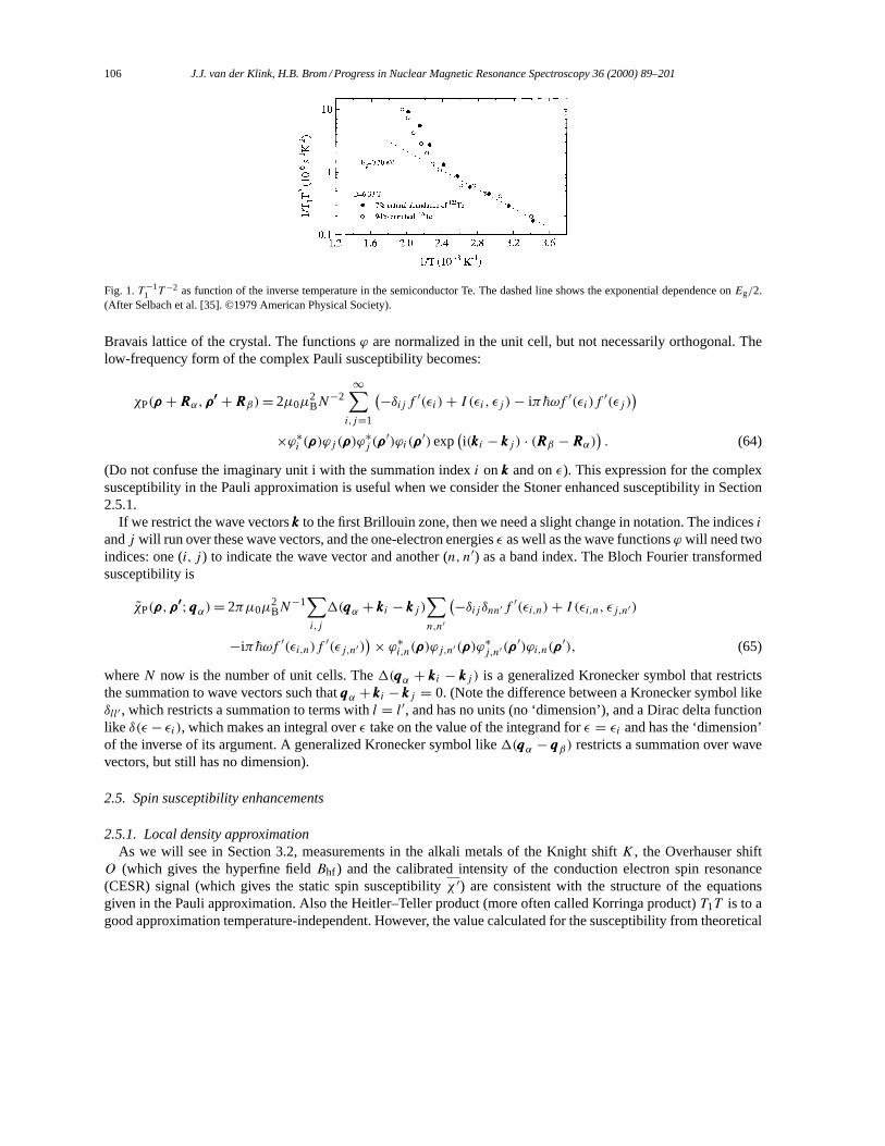
Such a temperature dependence is measured in the semiconductor Te [35] below 400 K withEg = 0.30 eV (seeFig. 1).
Coming back to the subject of metals, we use thatf ′(εi) ≈ −δ(εi − Ef ) and the density of statesD(Ef ) (twicethe number of energy levels at the Fermi energy, normalized per electron) to write
χ ′P = µ0µ2B�−1D(Ef ) with D(Ef ) = 2N−1
∞∑i=1
δ(εi − Ef ). (63)
The periodicity of the crystal lattice means that the one-electron functionsφ(rrr) can be chosen in the Bloch form:φ(ρρρ + RRRα) = N−1/2ϕ(ρρρ)exp(ikkk · RRRα) with ρρρ restricted to the unit cell in the origin, andRRRα a vector in the
106 J.J. van der Klink, H.B. Brom / Progress in Nuclear Magnetic Resonance Spectroscopy 36 (2000) 89–201
Fig. 1.T −11 T −2 as function of the inverse temperature in the semiconductor Te. The dashed line shows the exponential dependence onEg/2.
(After Selbach et al. [35]. ©1979 American Physical Society).
Bravais lattice of the crystal. The functionsϕ are normalized in the unit cell, but not necessarily orthogonal. Thelow-frequency form of the complex Pauli susceptibility becomes:
χP(ρρρ +RRRα,ρ′ρ′ρ′ +RRRβ)= 2µ0µ2BN−2∞∑
i,j=1
(−δij f ′(εi)+ I (εi, εj )− iπ~ωf ′(εi)f ′(εj ))
×ϕ∗i (ρρρ)ϕj (ρρρ)ϕ∗j (ρρρ′)ϕi(ρρρ′)exp(i(kkki − kkkj ) · (RRRβ −RRRα)
). (64)
(Do not confuse the imaginary unit i with the summation indexi onkkk and onε). This expression for the complexsusceptibility in the Pauli approximation is useful when we consider the Stoner enhanced susceptibility in Section2.5.1.
If we restrict the wave vectorskkk to the first Brillouin zone, then we need a slight change in notation. The indicesi
andj will run over these wave vectors, and the one-electron energiesε as well as the wave functionsϕ will need twoindices: one (i, j ) to indicate the wave vector and another (n, n′) as a band index. The Bloch Fourier transformedsusceptibility is
χP(ρρρ,ρ′ρ′ρ′;qqqα)= 2πµ0µ
2BN−1∑i,j
1(qqqα + kkki − kkkj )∑n,n′
(−δij δnn′f ′(εi,n)+ I (εi,n, εj,n′)−iπ~ωf ′(εi,n)f ′(εj,n′)
)× ϕ∗i,n(ρρρ)ϕj,n′(ρρρ)ϕ∗j,n′(ρρρ′)ϕi,n(ρρρ′), (65)
whereN now is the number of unit cells. The1(qqqα + kkki − kkkj ) is a generalized Kronecker symbol that restrictsthe summation to wave vectors such thatqqqα + kkki − kkkj = 0. (Note the difference between a Kronecker symbol likeδll′ , which restricts a summation to terms withl = l′, and has no units (no ‘dimension’), and a Dirac delta functionlike δ(ε − εi), which makes an integral overε take on the value of the integrand forε = εi and has the ‘dimension’of the inverse of its argument. A generalized Kronecker symbol like1(qqqα − qqqβ) restricts a summation over wavevectors, but still has no dimension).
2.5. Spin susceptibility enhancements
2.5.1. Local density approximationAs we will see in Section 3.2, measurements in the alkali metals of the Knight shiftK, the Overhauser shift
O (which gives the hyperfine fieldBhf ) and the calibrated intensity of the conduction electron spin resonance(CESR) signal (which gives the static spin susceptibilityχ ′) are consistent with the structure of the equationsgiven in the Pauli approximation. Also the Heitler–Teller product (more often called Korringa product)T1T is to agood approximation temperature-independent. However, the value calculated for the susceptibility from theoretical
J.J. van der Klink, H.B. Brom / Progress in Nuclear Magnetic Resonance Spectroscopy 36 (2000) 89–201 107
density of states curves does not agree particularly well; neither does the Korringa relation between the squareof the shift and relaxation rate given by Eq. (58). Furthermore in the Pauli approximation the total shift must benecessarily positive, since the (spin) Knight shift is positive, and the net orbital shift is expected to be either verysmall, or dominated by the positive van Vleck contribution. However, in some transition metals (Pt, Pd) the shift isbeyond doubt negative.
These problems are solved in the present approximation, where we use the expressions for susceptibility enhance-ment as given by density-functional theory. (We use these expressions to show a change in structure of the equationsonly; not to perform actual calculations). This enhancement gives at the same time three effects: a Stoner-likeamplification [36] of the static susceptibility; a Moriya-type desenhancement factor [37] in the Korringa relation;and the Yafet–Jaccarino kind of core-polarization hyperfine fields [38], that may be parallel or antiparallel to theapplied field.
The density-functional theory of the inhomogeneous electron gas [39–42] says that in the local-density approxi-mation the paramagnetic susceptibility can be written in the form of an integral equation:
χ(ρρρ,ρρρ′ +RRRα) = χP(ρρρ,ρρρ′ +RRRα)+
∑β
∫cellχP(ρρρ,ρρρ1+RRRβ)ν(n(ρρρ1+RRRβ))χ(ρρρ1+RRRβ,ρρρ′ +RRRα)dρρρ1, (66)
whereν(n(rrr)) is related to a second derivative of the exchange-correlation energy, and is (in the local-densityapproximation) a function only of the charge densityn in the pointrrr. The quantityχP(ρρρ,ρρρ
′ +RRRα) is the ‘nonin-teracting’ Pauli susceptibility, see Eq. (64). The vectorsρρρ′ andρρρ1 are in the unit cell at the origin, andRRRα andRRRβare lattice vectors, as introduced in Eq. (30). For simplicity,ν(n(rrr)) will be writtenν(ρρρ) in the following, with thevectorρρρ in the unit cell at the origin (the charge density having, of course, the periodicity of the lattice).
The equivalent equation for the Bloch Fourier transformed susceptibilities is (compare Eq. (31))
χ(ρρρ,ρρρ′; Eqqqα) = χP(ρρρ,ρρρ′;qqqα)+
∫cellχP(ρρρ,ρρρ1;qqqα)ν(ρ1)χ(ρρρ1,ρρρ
′;qqqα)dρρρ1. (67)
The expression for the real part of the susceptibility is directly obtained by adding a prime to allχ in Eq. (66) andEq. (67). But for later use we also write it in a slightly different form, using that the susceptibility should obey thereciprocity relationχ(rrr1, rrr2) = χ(rrr2, rrr1):
χ ′(ρρρ,ρρρ′ +RRRα) = χ ′P(ρρρ′ +RRRα,ρρρ)+∑β
∫cellχ ′P(ρρρ
′ +RRRα −RRRβ,ρρρ1)ν(ρρρ1)χ′(ρρρ1+RRRβ,ρρρ)dρρρ1. (68)
Once theχ ′ has been found, theχ ′′ can be obtained to lowest order in~ω from
χ ′′(ρρρ,ρρρ′ +RRRα) = χ ′′P(ρρρ,ρρρ′ +RRRα)+ 2∑β
∫cellχ ′′P(ρρρ,ρρρ1+RRRβ)ν(ρρρ1)χ
′(ρρρ1+RRRβ,ρρρ′ +RRRα)dρρρ1
+∑β,γ
∫ ∫cellχ ′(ρρρ,ρρρ1+RRRβ)ν(ρρρ1)χ
′′P(ρρρ1+RRRβ,ρρρ2+RRRγ )ν(ρρρ2)χ
′(ρρρ2+RRRγ ,ρρρ′ +RRRα)dρρρ1 dρρρ2, (69)
and the Bloch Fourier transform of this equation is
χ ′′(ρρρ,ρρρ′;qqqα) = χ ′′P(ρρρ,ρρρ′;qqqα)+ 2∫
cellχ ′′P(ρρρ,ρρρ1;qqqα)ν(ρρρ1)χ
′(ρρρ1,ρρρ′;qqqα)dρ1
+∫ ∫
cellχ ′(ρρρ,ρρρ1;qqqα)ν(ρρρ1)χ
′′P(ρρρ1,ρρρ2;qqqα)ν(ρρρ2)χ
′(ρρρ2,ρρρ′;qqqα)dρρρ1 dρρρ2. (70)
In numerical work, the equation can be applied to crystals with several different atoms in the unit cell (e.g.YBa2Cu3O7, see [43]), but here we will simplify to a system with one atom per unit cell in a cubic structure.
108 J.J. van der Klink, H.B. Brom / Progress in Nuclear Magnetic Resonance Spectroscopy 36 (2000) 89–201
We will take the Wigner–Seitz cell as the unit cell, approximate it by a sphere, and assume that the spin density andthe charge density have spherical symmetry, replacingρρρ by ρ, and dρρρ by 4πρ2dρ. The wave functionsϕi(ρρρ) in Eq.(64) are developed in spherical harmonicsYml (θ, φ):
ϕi(ρρρ) = (4π)1/2∞∑l=1
+l∑m=−l
Clm(i)ϕl(εi, ρ)Yml (θ, φ), (71)
where the radial functionϕl(εi, ρ) (do not confuse with the total functionϕi(ρρρ)) which can be taken as real, anddepends on the indexi only through the energyεi of the one-electron state described by the wave functionϕi(ρρρ).The spherical harmonics are orthonormal:∫ 2π
φ=0
∫ π
θ=0Ym∗l (θ, φ)Ym
′l′ (θ, φ) sin(θ)dθ dφ = δll′δmm′ , (72)
the radial wave functions are normalized as
4π∫ WS
0ρ2|ϕl(ε, ρ)|2 dρ = 1, (73)
where WS is the radius of the Wigner–Seitz sphere, and the coefficients are normalized as
∞∑l=1
+l∑m=−l|Clm(i)|2 = 1. (74)
In the expression for the complex Pauli susceptibility, Eq. (64), we replace the product of two wave functions takenin the same pointρρρ by its spherical average:
ϕ∗i (ρ)ϕj (ρ) ≈ (4π)−1∫ 2π
φ=0
∫ π
θ=0ϕ∗i (ρρρ)ϕj (ρρρ) sin(θ)dθ dφ =
∑lm
C∗lm(i)Clm(j)ϕl(εi, ρ)ϕl(εj , ρ). (75)
Likewise, we will assume that the enhanced susceptibility is given in terms of such spherical averages.Thelm-like partial density of electron states at energyε (twice the number of energy levels per atom and per unit
energy interval)Dlm(ε) is related to the set of complex expansion coefficientsClm(i) through Obata’s sum rule[44]:
2N−1∞∑i=1
δ(ε − εi)C∗lm(i)Cl′m′(i) = δll′δmm′Dlm(ε), (76)
whereN is the number of unit cells. Note that on both sides of Eq. (76) the dimension is 1/energy.Since the spherical harmonics form a complete set, the expansions given in Eqs. (71),(73) and (74) are formally
exact; but of course they will be useful only if it turns out that a small number ofl-values is sufficient for a correctrepresentation of theϕi(ρρρ). These wave functions may be ‘hybridized’ in the sense that they do not need to be purelys-like or d-like, or other; only the average value|Clm|2 of the projection constants appears in the expression for thepartial densities of state. This formulation in real space does not require to group the one-electron eigenfunctionsin bands, as is done in the Bloch Fourier transform Eq. (65).
In order to proceed further, we will need, however, some other assumptions in addition to the sphericalaverages. Letm(ρ) be a quantity proportional to the magnetization created in pointρρρ by a uniform field, anddefined as
m(ρ) =N∑α=1
∫cellχ ′(ρ,ρρρ′ + rrrα)dρρρ′. (77)
J.J. van der Klink, H.B. Brom / Progress in Nuclear Magnetic Resonance Spectroscopy 36 (2000) 89–201 109
Setting−f ′(ε) = δ(ε − Ef ) in the expression forχ ′P, Eq. (64), and using Eq. (68) we obtain
m(ρ) = µ0µ2B
∑lm
Dlm(Ef )
(ϕ2l (Ef , ρ)+
N∑α=1
∫cellϕ2l (Ef , |ρ′ρ′ρ′|)ν(ρρρ′)χ ′(ρρρ′ +RRRα, |ρρρ|)dρρρ′
). (78)
The contact Knight shift for the nucleus inρ = 0, therefore, has a direct contribution, proportional to the first termwithin parentheses on the right (and nonzero only forl = 0), and a core polarization contribution given by thesecond term.
In the following we attempt to decompose the static susceptibility, the Knight shift and the relaxation rateapproximately into sums oflm-like contributions [38,45]. It will be convenient to introduce a quantity
ml(ρ;qqqα) = ϕ2l (Ef , ρ)+
N∑β=1
exp(iqqqα ·RRRβ)∫
cellϕ2l (Ef , |ρ′ρ′ρ′|)ν(ρρρ′)χ ′(ρρρ′ +RRRβ, |ρρρ|)dρρρ′. (79)
The uniform susceptibility is
χ ′ = �−1∫
4πρ2m(ρ)dρ = µ0µ2B�−1∑lm
Dlm(Ef )
∫4πρ2ml(ρ;0)dρ =
∑lm
χ ′lm, (80)
which defines the partial susceptibilitiesχ ′lm. The enhancement with respect to the Pauli valueχ ′P,lm is given by
χ ′lmχ ′P,lm
=∫
4πρ2ml(ρ;0)dρ = 1
1− αl , (81)
where the right most expression defines thel-like partial Stoner factorαl .The Knight shiftK(0) is
K(0) = 2
3m(0) =
∑lm
χ ′lm�Bhf,l(0)
µ0µB=∑lm
Klm(0), (82)
where the last equality defines the partial contributions to the shift, and the effectivel-like hyperfine fieldBhf,l isdefined as
�Bhf,l(0)
µ0µB= 2ml(0;0)
3�−1∫
4πρ2ml(ρ;0)dρ. (83)
This hyperfine field can be nonzero also forl 6= 0, and the sign ofml(ρ;0) in ρ = 0 (the numerator) may beopposed to that of its average over the Wigner–Seitz sphere (the denominator), giving a negative hyperfine field.
To separateχ ′′(0,0), that appears in the expression for the relaxation rate, Eq. (43), intolm-like contributions,we make the approximation that in the enhancement integrals in Eq. (69) only those terms in the sums give animportant contribution where both arguments ofχ ′′P(rrr1, rrr2) are in the same unit cell:
χ ′′(0,0) ≈ χ ′′P(0,0)+ 2∫
cellχ ′′P(0,ρρρ1)ν(ρρρ1)χ
′(ρρρ1,0)dρρρ1
+∑β
∫ ∫cellχ ′(0,ρρρ1+RRRβ)ν(ρρρ1)χ
′′P(ρρρ1+RRRβ,ρρρ2+RRRβ)ν(ρρρ2)χ
′(ρρρ2+RRRβ,0)dρρρ1 dρρρ2. (84)
Introducing the spherical-average expression forχ ′′P(ρ1, ρ2)
χ ′′P(ρρρ1+RRRβ,ρρρ2+RRRβ) = χ ′′P(ρρρ1,ρρρ2) = χ ′′P(ρ1, ρ2) = 1
2π~ωµ0µ
2B
∑lm
D2lm(Ef )ϕ
2l (Ef , ρ1)ϕ
2l (Ef , ρ2), (85)
110 J.J. van der Klink, H.B. Brom / Progress in Nuclear Magnetic Resonance Spectroscopy 36 (2000) 89–201
the relaxation rate can be written as
S(T1T )−1 =
∑lm
klK2lm, (86)
where the partial contribution to the Knight shiftKlm have been defined in Eq. (82), and where the ‘desenhancementfactor’ kl is given by
k−1l =
|ml(0,0)|2N−1
∑Nα=1|ml(0;qqqα)|2
. (87)
Thekl are commonly called desenhancement factors, but in some cases they actually represent an increase in relax-ation rate with respect to the Korringa-like value. It depends on whether the average value of|ml(0;qqqα)|2 is larger orsmaller than its value forqqqα = 0. When the most importantml(0;qqqα) occurs at zero wave vector, the magnetizationis aligned over many unit cells, and therefore ferromagnetic: the factorkl < 1. In the opposite case, when the biggestml(0;qqqα) is found well away fromqqqα = 0, the magnetization changes sign over distances comparable to a unit celldimension and therefore it represents an antiferromagnetic magnetization: in that casekl > 1.
The desenhancement factor for the homogeneous electron gas has been discussed by Moriya [37]. Because ofthe homogeneity there are no indiceslm, m(ρρρ;qqq) is independent ofρρρ, and the hyperfine field is simplyBhf =2µ0µB/3� (although different values are usually supplied in an ad-hoc manner). Theν(ρρρ) is taken proportional toδ(ρρρ) and theq-dependence ofm(ρρρ;qqq) becomes of the Lindhard form, i.e. has its maximum atqqq = 0, and thereforea desenhancement is found.
The right-hand sides of Eqs. (80),(82) and (86) are explicitly labeled with a given value ofl (andm). Assume forthe sake of argument that in a given system, perhaps a transition metal alloy, we can experimentally varyD00(Ef ),without affecting any of theD2m(Ef ); would all quantities labeled withl = 2 remain completely unchanged? Thisis only approximately true, as we will show on the example of the uniform susceptibility. From now on, we will nolonger show the argumentEf in the quantitiesDlm(Ef ) andϕl(Ef , ρ). Using Eq. (79) the enhancement factor inEq. (81) is written as∫
4πρ2ml(ρ;0)dρ = 1+∫
4πρ′2ϕ2l (ρ′)ν(ρ′)m(ρ′)dρ′
= 1+ µ0µ2B
∑l′m′Dl′m′
∫4πρ2ϕ2
l (ρ)ν(ρ)ml′(ρ;0)dρ. (88)
Now approximate theml(ρ;0) in the leftmost and right most integrals in Eq. (88) by a function of the form(1+ Al)ϕ2
l (ρ), where the constantAl remains to be determined; Eq. (88) transforms into
1+ Al =∫
4πρ2ml(ρ;0)dρ = 1+ µ0µ2B
∑l′m′Dl′m′(1+ Al′)
∫4πρ2ϕ2
l (ρ)ν(ρ)ϕ2l′(ρ)dρ
= 1+∑l′m′Dl′m′(1+ Al′)νll′ , (89)
where the last line defines the exchange integralsνll′ . Only if the diagonal elements ofνll′ are more important thanthe off-diagonal ones,νll′ ≈ νllδll′ , can we write a Stoner-like expression where the partial Stoner factorαl (seeEq. (81)) is determined only byl-like quantities:
χ ′ =∑lm
χ ′lm = µ0µ2B�−1∑lm
Dlm
1− νll∑m′Dlm′
. (90)
In applications of equations forχ ′, K andT1T with the structure derived here, it is usual to assume that theνllandBhf,l are properties of an atom in its Wigner–Seitz cell, and that, if we put this Wigner–Seitz cell in different
J.J. van der Klink, H.B. Brom / Progress in Nuclear Magnetic Resonance Spectroscopy 36 (2000) 89–201 111
environments, these intra-atomic exchange integrals and effective hyperfine fields do not vary much: the changes inenvironment will only change the densities of statesDlm. In systems that lack translation symmetry (surfaces, smallparticles), the different environments are described by differentlocal densities of states. The values of the exchangeconstants and hyperfine fields are often obtained once and for all by fitting data obtained in the bulk elemental metalof interest. (Calculated densities of states for the bulk are believed to be reliable, and are used as input parameters inthe fit). A good example of an important change in Wigner–Seitz cell with experimental conditions is given by thehigh pressure experiments on alkalis to be discussed in Section 3.2: here the cell volume changes very considerably,and the value of the hyperfine field does not remain constant.
2.5.2. Spin fluctuationsIn the treatment of Section 2.5.1, the exchange interaction, represented byνll in Eq. (90), has no effect on the
energy of the system when no magnetic field is applied: the system is completely ‘nonmagnetic’. (Of course someexchange-and-correlation potential has been used to determine the band structure, but that is completely independentof any magnetic-susceptibility effect). But strictly speaking, once an exchange coupling has been introduced, thereis a magnetic energy in zero applied field associated with the thermal fluctuations of the local spin density (around azero average). Simply stated, a thermal fluctuation sets up an internal field, and this field couples to the other modes.The free energy of the zero-field equilibrium state at a finite temperature now contains a contribution related tothe wave vector-dependent dynamic susceptibility of the system. Therefore, some kind of self-consistent proceduremust be followed to determine this susceptibility. For example, one could start from an enhancement found by alocal-density theory; write a spin–fluctuation term1F in the free energy using this susceptibility; add a magneticfield, and determine a new value of the susceptibility (the second derivative of the free energy with respect to thefield). Repeating the procedure should lead to a self-consistent value [46]. It is clear that this program is not easy toexecute, and no local-susceptibility variant exists: all available work is purely thermodynamic, yielding expressionsfor the low-frequency wave vector-dependent susceptibility, but not for the corresponding hyperfine fields.
It is plausible that at least a part of the contribution of the spin fluctuations to the susceptibility will be temperaturedependent. In the discussion here we only consider metals at temperatures sufficiently above their magnetic transitiontemperatures. Nevertheless, the wave vector-dependence of the strength of the spin fluctuations will reflect thecharacter of the ordered state: for simplicity we consider only ferro- and simple antiferromagnetic orderings. In ametal, these orderings are distinguished by saying that the frequency of the fluctuations in a certain wave vectorrange becomes very low when the transition temperature is approached from above, and finally these fluctuations‘freeze out’ (note that this is a dynamic mode, that slows down; which is not the same as creating a one-electronlocalized moment). The dynamic susceptibility at these wave vectors is temperature-dependent; but at wave vectorsfar away the susceptibility may well have a nearly Pauli-like temperature-independence. In the case of (what at lowtemperature will be) ferromagnets, the temperature dependence is nearqqq = 0, whereas in antiferromagnets it is forwave vectors about halfway into the Brillouin zone, since an antiferromagnetic unit cell has twice the dimensionsof its parent paramagnetic cell. It will be clear that temperature-dependent antiferromagnetic fluctuations can havean influence on the temperature dependence of theT1T -product, while at the same time the Knight shift could bedetermined by an (almost) temperature-independent long-wavelength susceptibility.
We can give here only the barest of outlines of the application of spin fluctuation theory to nuclear spin relaxation[47,48]. Consider that the magnetization in a sample fluctuates in time and varies in space:MMM(rrr, t). (We will notbother about unit cells and atoms). In the paramagnetic phase and in zero applied field:∫
sampleMMM(rrr, t)dV = 0=
∫ ∞t=0MMM(rrr, t)dt (91)
but the integrals of the squares of these quantities would be zero only if we had rigorouslyMMM(rrr, t) = 0 at all pointsand at all times. More precisely this idea is expressed by the space-time correlation function
〈MMM(rrr, t)MMM(rrr ′, t ′)〉 = FM(|rrr − rrr ′|, |t − t ′|) , (92)
112 J.J. van der Klink, H.B. Brom / Progress in Nuclear Magnetic Resonance Spectroscopy 36 (2000) 89–201
where the〈 〉 indicate a thermodynamic averaging, and the absolute-bars in the right-hand side come from theconditions of translational invariance and of stationarity. In a general caseFM is a tensor, but we consider onlyone diagonal component (and since our simple system is isotropic, all diagonal components behave the sameway). The double Fourier transform ofFM(rrr, t) is on one hand related to theqqq-dependent susceptibility (throughthe fluctuation-dissipation theorem and the Kramers–Kronig relations), and on the other hand to our postulatedcontribution1F to the free energy. Let the latter be expressed by an exchange interactionI (rrr − rrr ′) (the equivalentof νll in Eq. (90)):
1F = V −1∫ ∫
sampleI (rrr − rrr ′)MMM(rrr, t) ·MMM(rrr ′, t)drrr drrr ′ =
∫ ∫I (qqq)FM(qqq, ω)dqqq dω. (93)
It should be pointed out that the mechanism postulated by Eq. (93) does not contribute to the temperature dependenceof the susceptibility of a purely local-moment system. A local moment jumps (more or less) randomly between‘up’ and ‘down’, but its absolute value is temperature-independent (the jump rate need not be), so that Eq. (93)simply shifts the free energy by a constant amount. Spin–fluctuation theory [46] says that the magnetic momentper site in the ordered phase of a metallic system can be much smaller than oneµB, and that in the paramagneticphase the mean-squared moment grows approximately linearly in temperature. However, looking inqqq-space, thereis a difference between the paramagnetic phases of ferro- and antiferromagnetic systems. In ferromagnetic systems,the ‘ordering vector’QQQ is nearQQQ = 0, while for antiferromagnets it is some finite vector, usually denotedQQQA. Inqqq-space the increase with temperature ofFM(qqq, ω) in the paramagnetic phase is localized near an ordering vectorof the low-temperature phase.
The self-consistency requirement is now that the dynamical susceptibility calculated from the total free energy
Ft = F0 + FM(qqq;ω)+1F (94)
(whereF0 is the free energy without any magnetic field effects andFM(qqq;ω) is the magnetic free energy in the pres-ence of an applied field of wave vectorqqq and frequencyω) is the same as that calculated by the fluctuation–dissipationtheorem fromFM(qqq, ω). This of course is rather formidable, and cannot be done ab initio. The idea has been toparametrize a simple model, based on the electron gas, and then fit experimental results to parameters of the model.
In the context of NMR, the theory has mainly been used to discuss the difference in temperature dependence oftheT1T product for the paramagnetic phases of (incipient) ferromagnets and antiferromagnets. Because the rangeof qqq-vectors whereχ ′′(qqq, ω) changes with temperature is different in the two cases, the integral overχ ′′(qqq, ω)/ω,as in Eq. (44), behaves differently as well. To lowest order inqqq andω it has been found ([46], Eqs. 5.2 and 5.6) thatin the paramagnetic phases
χ ′′(QQQ+ qqq, ω)ω
∝ κ2
(q/qB)(κ2+ (q/qB)2)2(ferromagnets QQQ = 0) (95)
χ ′′(QQQ+ qqq, ω)ω
∝ κ2
(κ2+ (q/qB)2)2(antiferromagnetsQQQ =QQQA), (96)
whereqB is the radius of the effective, spherical Brillouin zoneqB = (6π2/�)1/3 with� the volume per magneticatom. The dimensionless parameterκ2 is proportional to the inverse of the enhancement by the spin fluctuations ofthe static susceptibility at the ordering wave vector:
κ2 ∝ χ ′0(QQQ,0)χ ′(QQQ,0)
(97)
and parametrizes the temperature dependence of the problem. It is found in spin fluctuation theory [46] that in theparamagnetic phases of both ferromagnets and antiferromagnets, sufficiently far from the transition temperaturethere is a region where theκ2 increases approximately linearly with temperature. Note, for antiferromagnets,
J.J. van der Klink, H.B. Brom / Progress in Nuclear Magnetic Resonance Spectroscopy 36 (2000) 89–201 113
the difference between the static uniform susceptibility (the response to a uniform applied field) and the staticsusceptibility at the ordering wave vector (response to an applied field with periodicityQQQA).
To lowest order, the temperature variation of(T1T )−1 is found by integratingq/qB in Eq. (95) or Eq. (96) over a
unit sphere, and retaining only the lowest power ofκ. The result is that in the paramagnetic phase of antiferromagnets(T1T )
−1 ∝ κ ∝ 1/√T and for ferromagnets(T1T )
−1 ∝ κ2 ∝ 1/T . In several weak (i.e. low transition temperature)ferromagnets and antiferromagnets such behavior has been identified in a well chosen temperature region.
2.6. Kramers’ degeneracy
2.6.1. Time reversal symmetryIn the Hartree picture, each energy eigenvalue is associated with two eigenfunctions that have the same orbital
parts, but ‘opposite’ spin parts. In solids, the orbital parts can be represented by Bloch functions. This leads to a veryconvenient formulation of the magnetic properties, since the Hamiltonian for the interaction between a magneticfield and an electron
H = µB
~BBB · (rrr ×ppp + 2sss) (98)
does not connect the two states, and the average value ofrrr ×ppp in each of the states is zero. Therefore, theg-factorhas exactly the free-electron value. By construction, the spin operatorsss has no matrix elements between statesbelonging to different pairs, but the orbital operatorrrr×ppp can have such elements (they appear e.g. in the expressionfor the orbital Knight shift, Eq. (25)).
This two-fold degeneracy is a special result of a theorem due to Kramers: if the Hamiltonian of any system withan odd number of electrons contains only kinetic-energy and electrostatic terms, then at least two-fold degeneracywill always exist. This degeneracy is lifted by additional Hamiltonian terms that contain a magnetic field. Theone-electron Hartree Hamiltonian is of course the simplest such case. The general situation is represented by an‘effective spin 1/2’, in the sense that there is a doublet of states; however, its energy splitting in the presence of anadditional magnetic field does not need to be the same as that of the ‘real spin 1/2’ of a free electron. To emphasizethis, we write the spin in the Pauli matrix notation, whereσσσ = 2sss/~ stands for the collection of the three matrices
σx =(
0 11 0
)σy = i
(0 −11 0
)σz =
(1 00 −1
). (99)
If the two degenerate states are represented by two orthonormal wave functions, these wave functions are related bythe ‘time-reversal’ operatorK. (The operation actually reverses the direction of all motion, both orbital and spin,rather than time). In the usual representation whererrr is diagonal and theσσσ defined as in Eq. (99), the time-reversaloperator is represented by
K = iσyK0, (100)
whereK0 is the ‘complex conjugation’ operator, that converts the spatial part of the wave function into its complexconjugate. It is easy to verify that(iσy)σσσ = −σσσ(iσy). In therrr-representation,ppp = (~/i)∇, and thusK0ppp = −pppK0.Therefore, the following anti-commutation rules hold:
Kσσσ = −σσσK (101)
K(rrr ×ppp) = −(rrr ×ppp)K. (102)
Let ψ1 andψ2 be any two wave functions for the odd-electron system, and let the corresponding ‘time-reversed’states beKψ1 andKψ2. To avoid ambiguities, we write the corresponding bras and kets as e.g.〈(Kψ1)| and|(Kψ1)〉.It follows from the usual definition of the scalar product〈ψ1|ψ2〉 that
〈ψ1|ψ2〉 = 〈(Kψ2)|(Kψ1)〉 (103)
114 J.J. van der Klink, H.B. Brom / Progress in Nuclear Magnetic Resonance Spectroscopy 36 (2000) 89–201
and therefore also that
〈ψ1|σσσ |ψ2〉 = 〈ψ1|(σσσψ2)〉 = 〈(Kσσσψ2)|(Kψ1)〉 = −〈(σσσKψ2)|(Kψ1)〉 = −〈(Kψ1)|σσσ |(Kψ2)〉∗. (104)
Let us now consider two members of a Kramers doublet at energyεi , denotedφi,α andφi,β and chosen orthogonalin the eigenfunction subspace belonging toεi such that
φi,α = Kφi,β . (105)
Choosingψ1 = ψ2 = φi,α in Eq. (104) it is easy to see that
〈φi,α|σσσ |φi,α〉 = −〈φi,β |σσσ |φi,β〉. (106)
In a similar way it can be shown that
〈φi,α|rrr ×ppp|φi,α〉 = −〈φi,β |rrr ×ppp|φi,β〉. (107)
In the simplest case, the two functionsφi,α andφi,β are pure ‘spin-up’ and ‘spin-down’ functions. The more generaldegeneracy that can exist (the ‘mixing’ of the pure spin states) is due to the existence of a spin–orbit couplingmechanism. A classical image of this coupling, which overestimates it by a factor of two, is as follows. An electronrunning at speedvvv through an electric fieldEEE senses a magnetic fieldBBB ′ given (to first order invvv/c) by
BBB ′ = − vvvc2×EEE (108)
and the magnetic dipole associated with the spin senses thisBBB ′. The fieldEEE is due to the (periodic) electrostaticpotential of the lattice. It is strongest in the core regions of the atoms; and becomes stronger if the core containsmore charge (i.e. when the atom is heavier). If an external magnetic field is applied,mvvv = ppp + eAAA, see Eq. (143)in Section 2.7. The Hamiltonian becomes
H = 1
2m(ppp + eAAA)2− eV + ~µB
2mc2σσσ ·EEE × (ppp + eAAA)+ µB
~BBB · (rrr ×ppp + ~σσσ). (109)
The term in the spin–orbit coupling containing the magnetic vector potential can be neglected. First, we consider thezero-field case, and takeHso = (~µB/2mc2)σσσ ·EEE×ppp as a perturbation on the states|i〉 of the Hartree HamiltonianH0 = (1/2m)ppp2− eV , resulting in states|i, so〉 given by
|i, so〉 = |i〉 +∑n
〈n|Hso|i〉εi − εn |n〉, (110)
where now|i, so〉 is one of the members of the Kramers doublet. Because of the properties discussed below Eq.(98) we can write theg-factor of this doublet as
gi |BBB|2= 〈i, so|BBB · (rrr ×ppp + ~σσσ)|i, so〉 = 〈i|~BBB · σσσ |i〉 +
∑n
〈n|Hso|i〉〈i|BBB · rrr ×ppp|n〉 + c.c.
εi − εn , (111)
where the c.c. stands for complex conjugate, and we have used that〈i|rrr × ppp|i〉 = 0 and〈i|σσσ |n〉 = 0. Here thesummation indexn runs over both ‘spin-up’ and ‘spin-down’ functions forn 6= i.
In an electron spin resonance experiment, we induce transitions between the two Kramers conjugate states. Thiscan only be done if initially the two states are not both full or both empty, that is, if the states are very close to theFermi energy. According to the above derivation, different pairs of states at the Fermi energy may have differentg-factorsgi . If the electron is scattered (e.g. by phonons) between different states at a rate fast compared to thecorresponding differences in Larmor frequencies, only an averageg-value is observed (just as in the case of rapidchemical exchange in NMR). The intensity of the ESR line is proportional to the number of participating states,
J.J. van der Klink, H.B. Brom / Progress in Nuclear Magnetic Resonance Spectroscopy 36 (2000) 89–201 115
which is proportional to the density of states at the Fermi energy, and therefore, to the Pauli susceptibilityχP. Sincethe averageg-value in metals is never very different from 2, it is in general not necessary to make ag-correction inthe expression forχP.
2.6.2. Shift, hyperfine fieldWe now want to see how this degeneracy affects the susceptibility and the Knight shift. For simplicity, we consider
the approximation where the Knight shift can be written as the product of a hyperfine field and a susceptibility. Inthis section we look at the hyperfine field; the next one is devoted to susceptibility effects. To discuss the hyperfinefield it is useful to have an expression for the two members of a Kramers doublet that shows explicitly the spatialand spin parts. It is easily verified that the followingφi,α andφi,β are connected byK (note thatK2 = −1):
φi,α = ϕa(rrr)(
10
)+ ϕ∗b (rrr)
(01
)(112)
φi,β = −ϕb(rrr)(
10
)+ ϕ∗a (rrr)
(01
), (113)
where the(10
)
are the eigenvectors of theσz-matrix. The simple Hartree picture is recovered whenϕb(rrr) = 0. We can choose thesewave functions so as to diagonalize the Zeeman HamiltonianHZ = (µB/~)BBB · (rrr ×ppp + ~σσσ):
〈φi,α|BBB · (rrr ×ppp + ~σσσ)|φi,α〉 = g|BBB|2
(114)
〈φi,α|BBB · (rrr ×ppp + ~σσσ)|φi,β〉 = 0 (115)
and the same with a minus sign when the indicesα andβ are exchanged. The hyperfine field is proportional to thematrix elements
BBBhf(rrr) ∝ 〈φi,α(rrr)|σzδ(rrr − rrr)|φi,α(rrr)〉 = |ϕa(rrr)|2− |ϕb(rrr)|2. (116)
In a simplified description, the (direct contact) Knight shift is proportional to the average of|BBBhf(0)| for states at theFermi energy, and toχP. The orbital Knight shift will be given by the usual expression, Eq. (25), but using the wavefunctionsφi,α etc. (This change in orbital Knight shift when the spin–orbit coupling is ‘switched on’ is sometimescalled the spin–orbit Knight shift). As a result of all this, one can expect fairly modest, quantitative, changes in theNMR quantities when spin–orbit coupling is taken into account.
However, there are two cases where the spin–orbit coupling is believed to modify qualitatively the behaviorexpected for the susceptibility in its absence. This is the subject of the next Section 2.6.3.
2.6.3. SusceptibilityFor BCS superconductors, one expects spin pairing at low temperatures, and therefore, also a vanishing contact
Knight shift [49], Eq. (35). An example of the same phenomenon in a cuprate superconductor [50] is given in Fig. 2.Something similar is supposed to occur in the quantum-size regime (see Section 4.1) of small metal particles with aneven number of electrons. Experimentally, such vanishing shifts are not always observed. For experimental reasons,NMR on superconducting metals must be performed on relatively fine powders. It is thought that in fine powdersand small particles the presence of the surface induces an additional spin–orbit coupling, resulting in one-electronwave functions of the type of Eqs. (112) and (113). It is then argued that a second-order effect in the spin-only
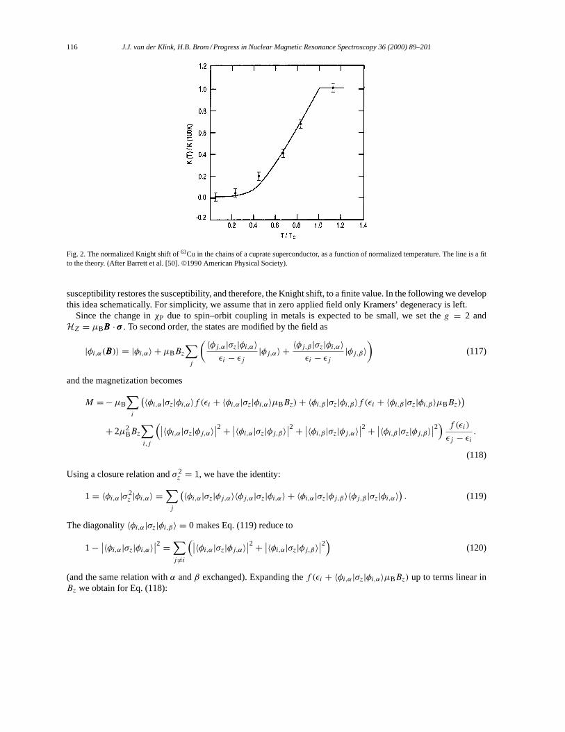
116 J.J. van der Klink, H.B. Brom / Progress in Nuclear Magnetic Resonance Spectroscopy 36 (2000) 89–201
Fig. 2. The normalized Knight shift of63Cu in the chains of a cuprate superconductor, as a function of normalized temperature. The line is a fitto the theory. (After Barrett et al. [50]. ©1990 American Physical Society).
susceptibility restores the susceptibility, and therefore, the Knight shift, to a finite value. In the following we developthis idea schematically. For simplicity, we assume that in zero applied field only Kramers’ degeneracy is left.
Since the change inχP due to spin–orbit coupling in metals is expected to be small, we set theg = 2 andHZ = µBBBB · σσσ . To second order, the states are modified by the field as
|φi,α(BBB)〉 = |φi,α〉 + µBBz∑j
( 〈φj,α|σz|φi,α〉εi − εj |φj,α〉 + 〈φj,β |σz|φi,α〉
εi − εj |φj,β〉)
(117)
and the magnetization becomes
M =−µB
∑i
(〈φi,α|σz|φi,α〉f (εi + 〈φi,α|σz|φi,α〉µBBz)+ 〈φi,β |σz|φi,β〉f (εi + 〈φi,β |σz|φi,β〉µBBz))
+ 2µ2BBz
∑i,j
(∣∣〈φi,α|σz|φj,α〉∣∣2+ ∣∣〈φi,α|σz|φj,β〉∣∣2+ ∣∣〈φi,β |σz|φj,α〉∣∣2+ ∣∣〈φi,β |σz|φj,β〉∣∣2) f (εi)
εj − εi .
(118)
Using a closure relation andσ 2z = 1, we have the identity:
1= 〈φi,α|σ 2z |φi,α〉 =
∑j
(〈φi,α|σz|φj,α〉〈φj,α|σz|φi,α〉 + 〈φi,α|σz|φj,β〉〈φj,β |σz|φi,α〉) . (119)
The diagonality〈φi,α|σz|φi,β〉 = 0 makes Eq. (119) reduce to
1− ∣∣〈φi,α|σz|φi,α〉∣∣2 =∑j 6=i
(∣∣〈φi,α|σz|φj,α〉∣∣2+ ∣∣〈φi,α|σz|φj,β〉∣∣2) (120)
(and the same relation withα andβ exchanged). Expanding thef (εi + 〈φi,α|σz|φi,α〉µBBz) up to terms linear inBz we obtain for Eq. (118):
J.J. van der Klink, H.B. Brom / Progress in Nuclear Magnetic Resonance Spectroscopy 36 (2000) 89–201 117
M
µ2BBz=− 2
∑i
f ′(εi)+∑
i,j, j 6=i
(∣∣〈φi,α|σz|φj,α〉∣∣2+ ∣∣〈φi,α|σz|φj,β〉∣∣2+ ∣∣〈φi,β |σz|φj,α〉∣∣2
+ ∣∣〈φi,β |σz|φj,β〉∣∣2)×(f (εi)− f (εj )
εj − εi + f ′(εi)). (121)
Here the first sum overi on the right-hand side gives the density of states at the Fermi energy,D(Ef ), compare Eq.(10). To be able to proceed further with the second sum, we assume that the matrix elements are mainly a functionof the energy difference between statesφi andφj , but do not depend (much) on these states themselves. In that casewe introduce a functiong(|εj − εi |) to rewrite Eq. (121) as
M
µ2BBz= D(Ef )+
∑i,j, j 6=i
g(|εj − εi |)(f (εi)− f (εj )
εj − εi + f ′(εi))
(122)
2.6.4. Metals, superconductors, small particlesNow we must make a distinction between the cases where there is a gap in the density of states atEf , as happens
at low temperature in superconductors or in ‘even’ small particles, and the usual situation, where the density ofstates is continuous atEf .
We treat the latter case first, and write
f (εi)− f (εj )εj − εi + f ′(εi) = −
∞∑n=2
(εj − εi)n−1
n!f (n)(εi), (123)
wheref (n)(εi) is thenth derivative off (ε), taken inε = εi . In Eq. (122) we can change the summation overj ina summation over energy intervalsεj − εi = 1ε:
M
µ2BBz= D(Ef )−
∞∑n=2
1
n!
∑1ε
g(|1ε|)(1ε)n−1∑i
f (n)(εi). (124)
Thenth derivatives are nonzero only in a small region around the Fermi energy, and we can replace the sum overi
by an integral:
∑i
f (n)(εi) = D(Ef )
∫ ∞0f (n)(ε)dε = D(Ef )
(f (n−1)(∞)− f (n−1)(0)
)= 0, (125)
which shows that there is no second-order spin susceptibility effect when the density of states is effectively constant(and nonzero) around the Fermi energy.
The case of a BCS superconductor at zero temperature will only be discussed briefly and qualitatively. Theelectrons pair off in the Kramers doublet states, giving a first-order spin susceptibility of zero. The density ofexcited states is nonzero only for excitation energies greater than the gap energy, usually denoted as 21. The Fermilevel is in the center of the gap, and therefore, Eq. (122) becomes
M
µ2BBz=
∑i,j, j 6=i
g(|εj − εi |)(f (εi)− f (εj )
εj − εi
). (126)
If g(|εj − εi |) is nonzero for|εj − εi | ≥ 21 then there will be a second-order contribution to the spin susceptibility,known as the Ferrell–Anderson effect [51,52]. This is believed to be the reason for the nonvanishing of the Knightshift in superconducting heavy nontransition metals such as Sn [49].
118 J.J. van der Klink, H.B. Brom / Progress in Nuclear Magnetic Resonance Spectroscopy 36 (2000) 89–201
In the quantum-size regime of ‘even’ small particles, the equal level spacing model (see Section 4.1) is easiestto handle. We have the same expression as in the superconductor case, Eq. (126), and now we let1 be the levelspacing. Then we number the levels such thatεi = i1 andεj = j1. Slightly rearranging the double sum we have
M
µ2BBz= 2
∑i,j, j 6=i
g(|j − i|1)(f (i1)− f (j1)
(j − i)1). (127)
Replacing the indexj by p = j − iM
µ2BBz= 2
∞∑p=1
g(p1)
p1
∞∑i=0
(f (i1)− f ((i + p)1)) . (128)
At low temperatures, wheref (ε) is a step function, the sum overi yieldsp, and thus, reintroducing the full expressionfor g(1ε) defined by Eq. (121) and Eq. (122):
M
µ2BBz=1−1
∑i,j, j 6=i
(∣∣〈φi,α|σz|φj,α〉∣∣2+ ∣∣〈φi,α|σz|φj,β〉∣∣2+ ∣∣〈φi,β |σz|φj,α〉∣∣2+ ∣∣〈φi,β |σz|φj,β〉∣∣2)
=1−1∑i
(1− ∣∣〈φi,α|σz|φi,α〉∣∣2+ 1− ∣∣〈φi,β |σz|φi,β〉∣∣2) = 2δi
(2− δi)1
, (129)
where we followed the literature [53] in defining〈φi,α|σz|φi,α〉 = 1− δi .
2.7. Appendix: second quantization
2.7.1. GeneralThe quantum mechanical wave function that represents a collection of electrons is antisymmetric with respect to
the operation that exchanges the space and spin coordinates of any pair of electrons in the collection (electrons arefermions). Let a set of orthonormal one-electron wave functions be given byφ1 · · ·φn, and let the system containN electrons, withN � n. Arrange a choice ofN (out ofn) functionsφi in anN ×N array where the elements in arow have constanti, while the arguments of the wave function are the same in any given column, all referring, say,to thekth electron. AnN -electron wave function satisfying the antisymmetry requirement can be represented bythe determinant of this array (called a Slater determinant). Ifn tends to infinity (as will be implied in all equationsof this Section), we can construct an infinite number of such arrays, and any desiredN -electron wave function canbe represented as a suitable linear combination of the determinants of such arrays. Of course it helps for simplicityto make a suitable choice for the collectionφi to start with; but here we will not actually make calculations, and weneed not go into this question.
In many practical problems, we want to determine matrix elements of a many-electron operator that has oneof two relatively simple structures: it can be written as a sum of terms that each contain only operators referringto one single electron (one-electron operators; e.g. terms in the kinetic energy), or only operators referring to twosingle electrons (two-electron operators; e.g. the interelectronic distance occurring in the Coulomb repulsion). Itcan be shown that such operators have elements only between determinantal wave functions differing by at most2 one-electron orbitals. For example, the first array may be constructed choosing allφi with 1 ≤ i ≤ N , and thesecond with 3≤ i ≤ N + 2. Because of this property, it turns out to be convenient to imagine a ‘creation’ operator
b†i , that ‘places’ an electron intoφi , and its Hermitian conjugatebi , the ‘destruction’ operator, that ‘removes’ an
electron from that orbital. In the example above let the determinant of the first array be denoted11···N , and that ofthe second array by13···N+2, then
11···N = b†1b†2bN+1bN+2δ3···N+2. (130)
J.J. van der Klink, H.B. Brom / Progress in Nuclear Magnetic Resonance Spectroscopy 36 (2000) 89–201 119
As a further example, we evaluate the matrix element
〈11···N |b†mb†2bN+1bN+2|13···N+2〉 = δm,1, (131)
which is zero, unless the indexm equals 1. The creation operatorsb†j and annihilation operatorsbi obey theanti-commutation rules
b†j bi + bib†j = δij (132)
b†i b
†j + b†j b†i = 0 (133)
bibj + bjbi = 0 (134)
In the following, we consider the interaction of theN -electron system with the magnetic field as a perturbation onthe ground state of the zero-field HamiltonianH0. Suppose that, through a suitable choice of one-electron wavefunctionsφi , the ground state ofH0 can be written as a single determinantal wave function, represented by a ket|90〉,with eigenvalueE0 forH0. Let other possible arrays that can be formed from the collection ofφi be represented bykets|9e〉, with eigenvaluesEe forH0. LetF andG be two one-electron operators:
F =n∑
k,l, k 6=lFklb
†k bl, G =
n∑i,j, i 6=j
Gij b†i bj (135)
and suppose thatFkl = F ∗lk andGij = G∗ji . In perturbation theory we encounter expressions of the type
∞∑e=1
〈90|G|9e〉〈9e|F |90〉 + c.c.
Ee − E0=
n∑k,l=1
n∑i,j=1
∞∑e=1
FklGij 〈90|b†i bj |9e〉〈9e|b†k bl |90〉 + c.c.
Ee − E0, (136)
where c.c. stands for complex conjugate. The product of the two matrix elements is nonzero only ifk = j andl = i;in that caseEe − E0 = εj − εi , whereεi is the one-electron energy corresponding to an electron ‘annihilated’ by
bi , andεj corresponds to an electron ‘created’ byb†j . Next we use the closure relation
∞∑e=1
|9e〉〈9e| = 1− |90〉〈90| (137)
to obtain for the perturbation expression, Eq. (136)
n∑i,j=1
FjiGij 〈90|b†i bj b†j bi |90〉 + c.c.
εj − εi =n∑
i,j=1
FjiGij 〈90|(1− b†j bj )b†i bi |90〉 + c.c.
εj − εi . (138)
A matrix element like〈90|b†i bi |90〉 is interpreted as the probability that the one-electron orbitalφi is occupied intheN -electron state90, and this probability is given by the Fermi–Dirac functionf (εi). Using, furthermore, theHermitian property of the matricesFkl andGij we have finally
∞∑e=1
〈9e|F |90〉〈90|G|9e〉 + c.c.
Ee − E0=
n∑i,j=1
I (εi, εj )FjiGij , (139)
with the definition thatI (εi, εj ) = 0 if εi = εj and(f (εi)− f (εj ))/(εj − εi) otherwise.
120 J.J. van der Klink, H.B. Brom / Progress in Nuclear Magnetic Resonance Spectroscopy 36 (2000) 89–201
2.7.2. Current densityThe current density operatorj0(rrr) for anN -electron system (the index 0 indicates that no magnetic field is
applied in this case) is given by
j0(rrr) =N∑i=1
−e2m(pppiδ(rrr − rrr i )+ δ(rrr − rrr i )pppi). (140)
To make a clear distinction between the continuous space variablerrr and the position operator of theith electronrrr i ,theˆ is used here to indicate operator quantities. We will not use this notation in general, however. The structure ofthis equation says that electroni does not contribute to the current density in pointrrr, unless its positionrrr coincideswith that point, in which case its contribution is(−e/m)ppp = −evvv, wheree is a positive quantity, and the current isopposed to the electron’s motion (this relation betweenmvvv andp is modified by the magnetic field, see below). Theoperatorj0(rrr) clearly is a one-electron operator in the sense given above. A general rule for the second-quantizationrepresentation of one-electron operators leads to
j0(rrr) = −e
2m
n∑k,l=1
〈φk|pppδ(rrr − rrr)+ δ(rrr − rrr)ppp|φl〉b†k bl, (141)
where the interesting feature is that the single sum over electrons in Eq. (140) has been replaced by a double sumover orbitals in Eq. (141). Of course the creation and annihilation operators will ensure that the correct numberof electronsN is used. The one-electron matrix elements in Eq. (141) are easy to evaluate using the explicitrepresentationppp = (~/i)∇:
〈φk|pppδ(rrr − rrr)+ δ(rrr − rrr)ppp|φl〉 = ~i
(φ∗k ∇φl − φl ∇φ∗k
), (142)
where the right-hand side is to be evaluated in the pointrrr (but we will not use this expression here).The HamiltonianH of a single electron in a magnetic vector potentialA and a scalar electric potentialV is given
by
H = 1
2m(ppp + eAAA)2− eV . (143)
From the change in the ‘kinetic energy’ term, we see that nowmvvv corresponds toppp + eAAA, thereby adding a termjAAA(rrr) to the current density operator, Eq. (141):
jAAA(rrr) = −e2
mAAA(rrr)δ(rrr − rrr) (144)
and in second quantization for theN -electron system:
jAAA(rrr) = −e2
mAAA(rrr)
n∑k,l=1
φ∗k (rrr)φl(rrr)b†k bl. (145)
In the Hartree approximation, the Hamiltonian of anN -electron system is a sum of terms like Eq. (143), the potentialV being due to the crystal lattice and the(N − 1) other electrons. ConsideringAAA as a perturbation, we write
H = H0 +HAAA, (146)
where, neglecting the terms inAAA2,
HAAA = −∫
j0(rrr) ·AAA(rrr)dV = e
2m
n∑k,l=1
〈φk|ppp ·AAA(rrr)+AAA(rrr) · ppp|φl〉b†k bl. (147)
Here the notationAAA(rrr) indicates thatAAA now takes the position operator of the electron as its argument.
J.J. van der Klink, H.B. Brom / Progress in Nuclear Magnetic Resonance Spectroscopy 36 (2000) 89–201 121
The ket|9AAA〉 representing theN -electron system in presence ofAAA can be written as
|9AAA〉 = |90〉 −∞∑e=1
〈9e|HAAA|90〉Ee − E0
|9e〉 (148)
and the current density in theN -electron system in the presence ofAAA is
jjj(rrr) = 〈9AAA|j0 + jAAA|9AAA〉. (149)
We requirejjj(rrr) to first order inAAA:
jjj(rrr) = 〈90|jAAA|90〉 −∞∑e=1
〈90|j0|9e〉〈9e|HAAA|90〉 + c.c.
Ee − E0. (150)
From the second quantization forms ofjAAA (Eq. (145)),HAAA (Eq. (147)) andj0 (Eq. (141)) and using Eq. (139) wefind
jjj(rrr)=n∑
i,j=1
(− e
2
2mAAA(rrr)δij f (εi)|φi(rrr)|2
+( e
2m
)2I (εi, εj )〈φi |pppδ(rrr − rrr)+ δ(rrr − rrr)ppp|φj 〉〈φj |AAA(rrr) · ppp + ppp ·AAA(rrr)|φi〉
). (151)
This completes the derivation of the current densityjjj(rrr) induced by an external vector potentialAAA(rrr). Note thatby definition the sums run over electron states, not over energy levels (the number of states is twice the number oflevels).
2.7.3. Spin magnetizationIn this section, it will be useful to have separate spin- and orbital indices to the creation and annihilation operators,
e.g.b†j↑. We will be interested in the representation of the components of the local spin magnetization operator
MMM(rrr), whererrr is a continuous space variable (not an electron position operatorrrr).
MMM(rrr) =N∑i=1
MMMiδ(rrr − rrri). (152)
The one-electron magnetic moment operator is related to the corresponding spin operator byMMMi = −2µBSSSi , becausespin and magnetic moment have opposite directions. The Bohr magnetonµB is the strength of an elementary dipole.The second-quantization representation of the irreducible tensor components ofMMM(rrr) is given by
M0 = µB
n∑k,l=1
(b†k↑bl↑ − b†k↓bl↓
)φ∗k (rrr)φl(rrr) (153)
M+1 = −µB√
2n∑
k,l=1
b†k↑bl↓φ
∗k (rrr)φl(rrr) (154)
M−1 = µB√
2n∑
k,l=1
b†k↓bl↑φ
∗k (rrr)φl(rrr), (155)
122 J.J. van der Klink, H.B. Brom / Progress in Nuclear Magnetic Resonance Spectroscopy 36 (2000) 89–201
where the indices↑ and↓ refer to magnetic moments parallel and antiparallel, respectively, to the magnetic field.The relation between Cartesian and irreducible tensor components is
M−1 = 12
√2(Mx − iMy), M0 = Mz, M+1 = −1
2
√2(Mx + iMy). (156)
The electron Zeeman Hamiltonian is
HZ = −∫M0(rrr)B0(rrr)dV = −µB
n∑k,l=1
(b†k↑bl↑ − b†k↓bl↓
)〈φk|B0(rrr)|φl〉, (157)
where the notationB0(rrr) indicates that the argument is the position operator of the electron. In a uniform field thisreduces to
HZ,0 = −µBB0
n∑k=1
(b†k↑bk↑ − b†k↓bk↓
). (158)
The magnetizationMz(rrr) is given to first order in the field by an expression rather similar to Eq. (150):
Mz(rrr) = 〈9BBB |M0(rrr)|9BBB〉 −∞∑e=1
〈9e|HZ|90〉〈90|M0(rrr)|9e〉 + c.c.
Ee − E0, (159)
where9BBB is the ground state in presence of the field, while90 and9e are evaluated without the field. In the firstterm we must, therefore, distinguish the one-electron energiesεi↑ andεi↓:
〈9BBB |b†i↑bj↑ − b†i↓bj↓|9BBB〉 = δij(f(εi − µB〈φi |B0(rrr)|φi〉
)− f (εi + µB〈φi |B0(rrr)|φi〉))
≈−2µBδij 〈φi |B0(rrr)|φi〉f ′(εi), (160)
wheref ′(εi) is the derivative of the Fermi–Dirac functionf (ε), taken inε = εi . In the sum over excited stateswe take the zero-field values forEe − E0, determined by one-electron energies likeεi andεj , and use the generalexpression, Eq. (139), so that finally
Mz(rrr) = 2µ0µ2B
n∑i,j=1
(−δij f ′(εi)+ I (εi, εj ))φ∗i (rrr)φj (rrr)∫
sampleφ∗j (rrr
′)HHH 0(rrr′)φi(rrr ′)drrr ′. (161)
This expression is used in the evaluation of the Knight shift and of the uniform susceptibility in the Pauli approxi-mation, Section 2.4.
2.7.4. Power absorptionTo study the average power absorbed by the spin magnetization from a nonuniform alternating fieldB0(rrr) cosωt
we consider the perturbation Hamiltonian
H1(t)=−∫M0(rrr)B0(rrr)
1
2(exp(iωt)+ exp(−iωt))dV
=−µB
2
n∑k,l=1
(b†k↑bl↑ − b†k↓bl↓
)〈φk|B0(rrr)|φl〉 (exp(iωt)+ exp(−iωt))
=H1,0 (exp(iωt)+ exp(−iωt)) , (162)
J.J. van der Klink, H.B. Brom / Progress in Nuclear Magnetic Resonance Spectroscopy 36 (2000) 89–201 123
where the last line defines the operatorH1,0. Using Fermi’s golden rule, we write the transition probability per unittimeW0e to go, under influence of this perturbation, from theN -electron ground state represented by the ket|90〉to an excited state represented by|9e〉 as
W0e(ω) = 2π
~
∣∣〈90|H1,0|9e〉∣∣2 δ(Ee − E0 + ~ω). (163)
To make the connection between this quantum mechanical result and thermodynamics is not straightforward. Clearly,if we are sure that the system is initially in the state|90〉 then its probability per unit time to go to the state|9e〉by absorption is given byW0e in Eq. (163). But if on the contrary we were sure that initially the system is in|9e〉, then the same expression gives the rateWe0 at which it goes to the state|90〉 by stimulated emission. So thethermodynamical average should take into account how likely it is to be initially in each of the states. SinceH1,0is a one-electron operator, this accounting can be done by considering separately processes where a one-electronstate at lower energy is ‘replaced’ by one at higher energy (absorption), and the opposite (stimulated emission). Thetotal rate of all absorption processes is
W0→(ω) =∑e
W0e(ω) = π
~µ2
B
n∑i,j=1
f (εi)(1− f (εj )
) ∣∣〈φi |B0(rrr)|φj 〉∣∣2 δ(εj − εi − ~ω) (164)
with εj > εi : in the initial state|φi〉 is occupied, and|φj 〉 is empty. The total rate of all emission processes isobtained when initially the higher-energy state is occupied, and the lower-energy one is empty:
W0←(ω) =∑e
We0(ω) = π
~µ2
B
n∑i,j=1
f (εj ) (1− f (εi))∣∣〈φj |B0(rrr)|φi〉
∣∣2 δ(εj − εi − ~ω) (165)
again withεj > εi . The net absorbed power is thus
P(ω)= ~ω (W0→(ω)−W0←(ω))
= (πω)µ2B
n∑i,j=1
(f (εi)− f (εj )
) ∣∣〈φi |B0(rrr)|φj 〉∣∣2 δ(εj − εi − ~ω), ~ω > 0. (166)
For our application we will be interested in the low-frequency limit ofP(ω)/~ω2. We use that
(f (εi)− f (εj )
)δ(εj − εi − ~ω) = −~ωf ′(εi)δ(εj − εi − ~ω), ~ω→ 0 (167)
and in Section 2.4 we need the limit
lim~ω→0
2P(ω)
~ω2= −2πµ2
B
n∑i,j=1
f ′(εi)δ(εj − εi − ~ω)∣∣〈φi |B0(rrr)|φj 〉
∣∣2
= −2πµ0µ2B
n∑i,j=1
f ′(εi)δ(εj − εi − ~ω)∫ ∫
sampleφ∗i (rrr)BBB(rrr)φj (rrr)φ
∗j (rrr′)HHH(rrr ′)φi(rrr ′)drrr drrr ′. (168)
According to this equation, no power is absorbed from a uniform fieldBBB0(rrr) = BBB0. Clearly, it does not describethe spin–lattice relaxation process when we switch on a magnetic field; such processes are in fact related to theevolution in time ofW0←(ω) andW0→(ω).
124 J.J. van der Klink, H.B. Brom / Progress in Nuclear Magnetic Resonance Spectroscopy 36 (2000) 89–201
3. NMR in metals
3.1. Zero of the shift scale
3.1.1. The reference stateThe very first review of NMR in metals [15] already pointed out the importance of the choice of reference
compound to determine the metallic shift. In Section 2.2 we have found the following expression for the orbitalKnight shift (see Eq. (25)):
Korb = −µ0e2
4πm
∞∑i=1
f (εi)
⟨φi
∣∣∣∣x2+ y2
2|r|3∣∣∣∣φi
⟩+ µ0e
2
4πm
∞∑i,j=1
I (εi, εj )
2m
⟨φi
∣∣∣∣ lz|r|3∣∣∣∣φj
⟩〈φj |lz|φi〉. (169)
Here the applied field has been taken in thez-direction, and|r|2 = x2 + y2 + z2; furthermore,lz = (rrr ×ppp)z. Thefirst term is diamagnetic (negative), the second one is paramagnetic, and often called the van Vleck shift, becauseit corresponds to a contribution to the magnetic susceptibility of ions that has first been discussed by van Vleck.(This susceptibility is often called temperature independent paramagnetism, TIP, by magnetochemists).
It is useful to divide the diamagnetic term into two parts. The first diamagnetic contribution is due to the low-lying(εi � Ef ) core electronic levels. It is generally assumed, and confirmed by recent ab-initio calculations of chemicalshifts [54], that this term is almost independent of atomic environment, and can be treated as a constant for a giventype of atom. The second diamagnetic contribution is that of valence electrons (εi ≈ Ef ). It is usually neglectedcompared to the paramagnetic shift which is caused by these same electrons. (Because of the factorI (εi, εj ) thecore electrons have no effect on paramagnetism). The van Vleck susceptibilityχvV is given by
χvV = µ0e2
4πm�−1
∞∑i,j=1
I (εi, εj )
2m
∣∣〈φi |lz|φj 〉∣∣2 (170)
and the second term in Eq. (169) is often rewritten in terms of this susceptibility and an orbital hyperfine fielddefined such that
KvV = χvV�Bhf,orb
µ0µB. (171)
It is then usual to define an average value〈r−3〉 by
〈r−3〉 =∑∞i,j=1I (εi, εj )〈φi |lz|r|−3|φj 〉〈φj |lz|φi〉∑∞
i,j=1I (εi, εj )∣∣〈φi |lz|φj 〉∣∣2 (172)
so that the orbital hyperfine field can be expressed as
Bhf,orb = µ0µB〈r−3〉. (173)
The ideal ‘reference state’ therefore, is the nucleus with core electrons, rather than the ‘bare’ nucleus. (The latterwas preferred by the nuclear physicists of the early days, who were interested in the gyromagnetic ratio as a nuclearproperty, and thought of shifts as a useless nuisance). For the alkalis, silver and some other metals it is possible tofind aqueous solutions of salts with noncoordinating anions, and extrapolate the observed resonance frequency toinfinite dilution to obtain a suitable reference.
For transition metals this usually does not work since even the coordination with water can already be fairly strong.Since the paramagnetic shift is related to the van Vleck paramagnetism, one might think of correlating the measuredmagnetic susceptibility and NMR shift in a series of ionic compounds. If we had some means of independently
J.J. van der Klink, H.B. Brom / Progress in Nuclear Magnetic Resonance Spectroscopy 36 (2000) 89–201 125
estimating the diamagnetic part of the susceptibility, then we could extrapolate the correlation plot to zero vanVleck paramagnetism, and find the resonance frequency for the ion with its core electrons only. Unfortunately, theestimate of the diamagnetic part usually cannot be made with sufficient precision.
A very elegant procedure has been proposed for ions that have paramagnetic groundstates when present asimpurities in simple host crystals, such as Co2+ in MgO ([55], p. 244). The idea is to observe the same ion in anumber of different hosts using a technique called electronic-nuclear double resonance (ENDOR). ENDOR detectsESR in the presence of an additional continuous frequency-swept decoupling in the NMR frequency range, andcontains information on the electronic as well as the nuclear transitions. The different ligand fields in the differenthost crystals will shift both the NMR and the ESR signals from their ‘free ion’ values. One could make a correlationplot of the observed nuclear and electronic frequencies, and extrapolate to the known ESR frequency at zero vanVleck susceptibility (corresponding tog ≈ 2): this gives the (unknown) NMR frequency without paramagneticcontribution. The experiment has never been performed in this complete form, but a simplified version, withoutextrapolation, has been used for the 3d5 ions Mn2+ and Fe3+ (it should also be applicable to Cr+). In these cases itis expected on theoretical grounds, and experimentally observed, that the ESR shift (with respect tog = 2) shouldbe small; therefore, the observed NMR frequency should also be close to the value at zero van Vleck susceptibility.The case of55Mn is discussed at some length in Section 3.7.1, and the result for57Fe will be briefly mentioned inSection 3.1.2.
For ions with nonmagnetic groundstates, a correlation between NMR and optical data can be used. The applicationof this method for the determination of the reference gyromagnetic ratio of several transition metal nuclei is thesubject of Section 3.1.2.
3.1.2. Optical methodsAmong the first clearly detected chemical shift differences were those for59Co in different ‘nonmagnetic’
compounds [56]. For simplicity, we will restrict our discussion mainly to octahedral complexes of d6 ions, likeCo3+. In an octahedral ligand field the five d-orbitals that are degenerate in energy in the atom are split in one groupof three, and another group of two. For a d6 ion in the ground state, the group of three is fully occupied and the groupof two is empty. The energy splitting often is fairly low, corresponding to optical frequencies in the visible region ofthe spectrum. Therefore, the energy denominators inI (εi, εj ) = (f (εi)−f (εj ))/(εj −εi) are relatively small, andthe shift according to Eq. (171) is important. It was observed that the59Co resonance in a series of such complexes isshifted to lower field (paramagnetic shift) when the optical transition occurs at longer wavelengths (lower energy):this correlation is called spectrochemical ordering [57,58]. In a number of Co complexes, the relation between shiftand wavelength is linear, so that extrapolation of the experimental straight line to zero wavelength (infinite energydifference, thereforeI (εi, εj ) → 0) should yield the zero of the NMR shift scale. This procedure supposes thatthe variation in excited-state energy in Eq. (170) is the determining variable, and that the geometric factor〈r−3〉in Eq. (172) is less important. However, this is not the general case, as we will see from data collected in Tables 1and 2.
In Table 1 the NMR shifts are given for195Pt, 103Rh, 59Co, 99Ru and57Fe in a series of d6 octahedral orquasi-octahedral complexes. The data are taken from [59], and given on the shift scales used in that book. So far asthe resonances have been observed, they all go from low field to high field in the order of ligands: F, H2O, OH, Cl,Br, ethane-1,2-diamine (abbreviated:en), CN and I, except for the inversion of Br andenfor 195Pt. The data for thesandwich compounds with cyclopentadienyl (Cp)2 show that the ligand-ordering idea can (in an imprecise way) beextended to other coordinations. The meaning of the values in the last line will be discussed below. We remark inpassing that on the shift scales used in Table 1, the resonance of Rh metal is at−1370 ppm, and that of Ru metal atapproximately+1500 ppm, refuting the idea that Knight shifts must be ‘unusually’ large. As we will see, the shiftsin the transition metals result from positive and negative contributions, that occasionally may cancel out.
The optical data in Table 2 show that spectrochemical ordering is indeed often observed, although there is anumber of exceptions, the most notable being the position of Cl and Br for195Pt and103Rh. Closer inspection ofthe numerical values also reveals that the linearity between shift and wavelength is usually much worse than for the
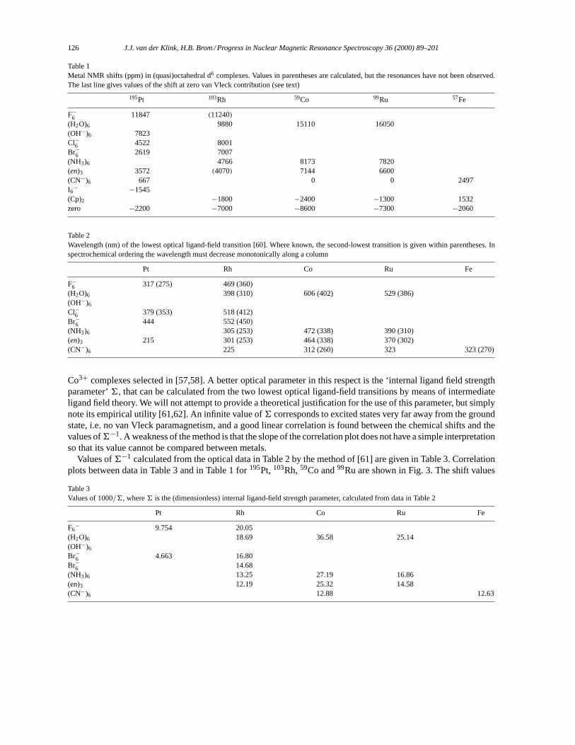
126 J.J. van der Klink, H.B. Brom / Progress in Nuclear Magnetic Resonance Spectroscopy 36 (2000) 89–201
Table 1Metal NMR shifts (ppm) in (quasi)octahedral d6 complexes. Values in parentheses are calculated, but the resonances have not been observed.The last line gives values of the shift at zero van Vleck contribution (see text)
195Pt 103Rh 59Co 99Ru 57Fe
F−6 11847 (11240)(H2O)6 9880 15110 16050(OH−)6 7823Cl−6 4522 8001Br−6 2619 7007(NH3)6 4766 8173 7820(en)3 3572 (4070) 7144 6600(CN−)6 667 0 0 2497I6− −1545
(Cp)2 −1800 −2400 −1300 1532zero −2200 −7000 −8600 −7300 −2060
Table 2Wavelength (nm) of the lowest optical ligand-field transition [60]. Where known, the second-lowest transition is given within parentheses. Inspectrochemical ordering the wavelength must decrease monotonically along a column
Pt Rh Co Ru Fe
F−6 317 (275) 469 (360)(H2O)6 398 (310) 606 (402) 529 (386)(OH−)6
Cl−6 379 (353) 518 (412)Br−6 444 552 (450)(NH3)6 305 (253) 472 (338) 390 (310)(en)3 215 301 (253) 464 (338) 370 (302)(CN−)6 225 312 (260) 323 323 (270)
Co3+ complexes selected in [57,58]. A better optical parameter in this respect is the ‘internal ligand field strengthparameter’6, that can be calculated from the two lowest optical ligand-field transitions by means of intermediateligand field theory. We will not attempt to provide a theoretical justification for the use of this parameter, but simplynote its empirical utility [61,62]. An infinite value of6 corresponds to excited states very far away from the groundstate, i.e. no van Vleck paramagnetism, and a good linear correlation is found between the chemical shifts and thevalues of6−1. A weakness of the method is that the slope of the correlation plot does not have a simple interpretationso that its value cannot be compared between metals.
Values of6−1 calculated from the optical data in Table 2 by the method of [61] are given in Table 3. Correlationplots between data in Table 3 and in Table 1 for195Pt, 103Rh, 59Co and99Ru are shown in Fig. 3. The shift values
Table 3Values of 1000/6, where6 is the (dimensionless) internal ligand-field strength parameter, calculated from data in Table 2
Pt Rh Co Ru Fe
F6− 9.754 20.05
(H2O)6 18.69 36.58 25.14(OH−)6
Br−6 4.663 16.80Br−6 14.68(NH3)6 13.25 27.19 16.86(en)3 12.19 25.32 14.58(CN−)6 12.88 12.63
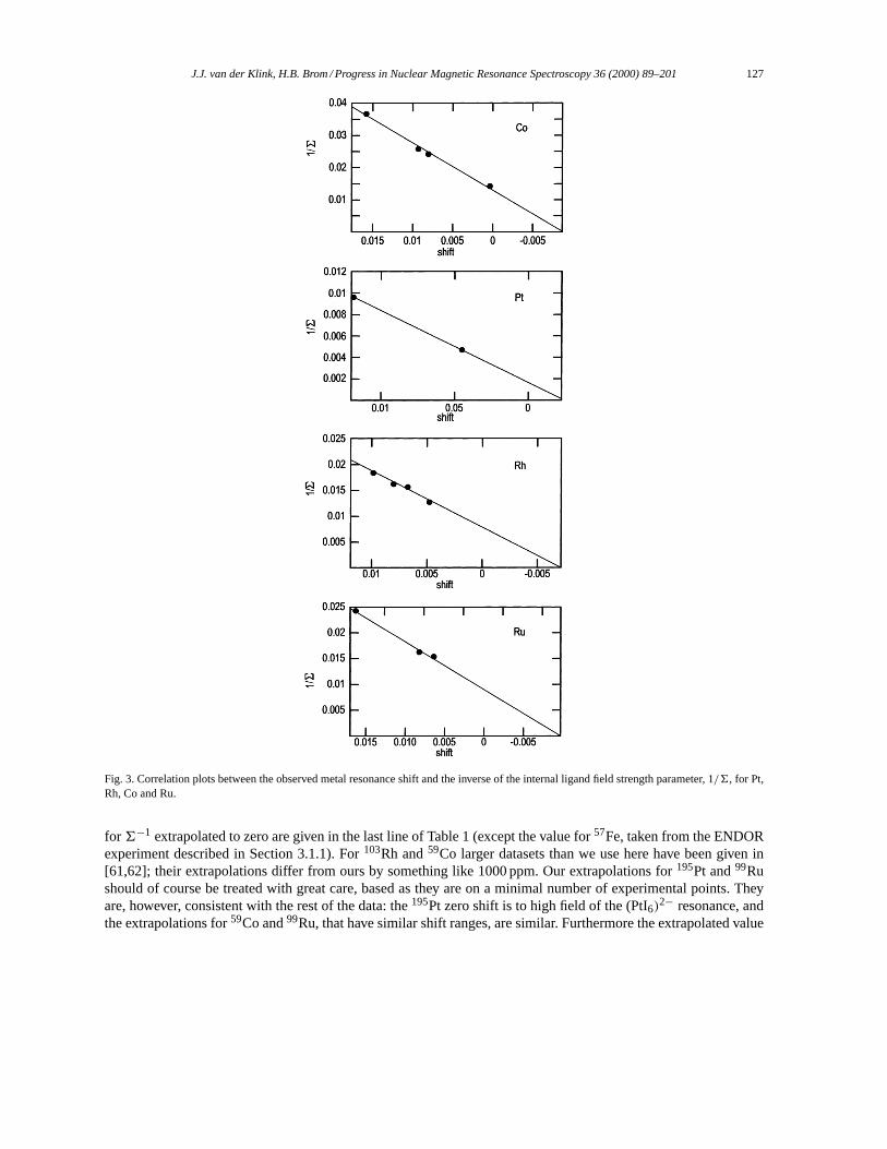
J.J. van der Klink, H.B. Brom / Progress in Nuclear Magnetic Resonance Spectroscopy 36 (2000) 89–201 127
Fig. 3. Correlation plots between the observed metal resonance shift and the inverse of the internal ligand field strength parameter, 1/6, for Pt,Rh, Co and Ru.
for 6−1 extrapolated to zero are given in the last line of Table 1 (except the value for57Fe, taken from the ENDORexperiment described in Section 3.1.1). For103Rh and59Co larger datasets than we use here have been given in[61,62]; their extrapolations differ from ours by something like 1000 ppm. Our extrapolations for195Pt and99Rushould of course be treated with great care, based as they are on a minimal number of experimental points. Theyare, however, consistent with the rest of the data: the195Pt zero shift is to high field of the (PtI6)
2− resonance, andthe extrapolations for59Co and99Ru, that have similar shift ranges, are similar. Furthermore the extrapolated value
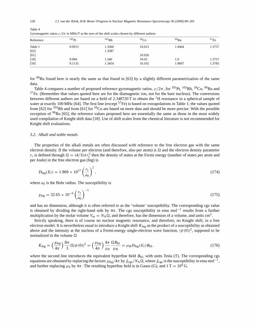
128 J.J. van der Klink, H.B. Brom / Progress in Nuclear Magnetic Resonance Spectroscopy 36 (2000) 89–201
Table 4Gyromagnetic ratiosγ /2π in MHz/T at the zero of the shift scales chosen by different authors
Reference 195Pt 103Rh 59Co 99Ru 57Fe
Table 1 9.0913 1.3360 10.015 1.9464 1.3757[62] 1.3387[61] 10.026[18] 9.094 1.340 10.03 1.9 1.3757[59] 9.1135 1.3454 10.102 1.9607 1.3785
for 99Ru found here is nearly the same as that found in [63] by a slightly different parametrization of the samedata.
Table 4 compares a number of proposed reference gyromagnetic ratios,γ /2π , for 195Pt, 103Rh,59Co,99Ru and57Fe. (Remember that values quoted here are for the diamagnetic ion, not for the bare nucleus). The conversionsbetween different authors are based on a field of 2.348720 T to obtain the1H resonance in a spherical sample ofwater at exactly 100 MHz [64]. The first line (except57Fe) is based on extrapolations in Table 1; the values quotedfrom [62] for 103Rh and from [61] for59Co are based on more data and should be more precise. With the possibleexception of99Ru [65], the reference values proposed here are essentially the same as those in the most widelyused compilation of Knight shift data [18]. Use of shift scales from the chemical literature is not recommended forKnight shift evaluations.
3.2. Alkali and noble metals
The properties of the alkali metals are often discussed with reference to the free electron gas with the sameelectron density. If the volume per electron (and therefore, also per atom) is� and the electron density parameterrs is defined through� = (4/3)πr3
s then the density of states at the Fermi energy (number of states per atom andper Joule) in the free electron gas (feg) is
Dfeg(Ef ) = 1.869× 10¹⁷(rs
a0
)2
, (174)
wherea0 is the Bohr radius. The susceptibility is
χfeg = 32.65× 10⁻⁶(rs
a0
)−1
(175)
and has no dimension, although it is often referred to as the ‘volume’ susceptibility. The corresponding cgs valueis obtained by dividing the right-hand side by 4π . The cgs susceptibility in emu mol−1 results from a furthermultiplication by the molar volumeVm = NA�, and therefore, has the dimension of a volume, and units cm3.
Strictly speaking, there is of course no nuclear magnetic resonance, and therefore, no Knight shift, in a freeelectron model. It is nevertheless usual to introduce a Knight shiftKfeg as the product of a susceptibility as obtainedabove and the intensity at the nucleus of a Fermi-energy single-electron wave function,|ψ(0)|2, supposed to benormalized in the volume�
Kfeg =(χfeg
4π
) 8π
3�|ψ(0)|2 =
(χfeg
4π
) 4π
µ0
�Bhf
µB= µBDfeg(Ef )Bhf , (176)
where the second line introduces the equivalent hyperfine fieldBhf , with units Tesla (T). The corresponding cgsequations are obtained by replacing the factorsχfeg/4π by χcgs/NA�, whereχcgsis the susceptibility in emu mol−1,and further replacingµ0 by 4π . The resulting hyperfine field is in Gauss (G), and 1 T= 104 G.
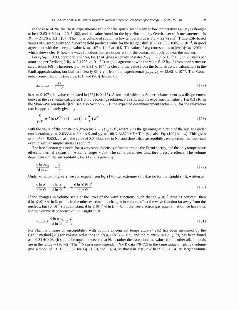
J.J. van der Klink, H.B. Brom / Progress in Nuclear Magnetic Resonance Spectroscopy 36 (2000) 89–201 129
In the case of Na, the ‘best’ experimental value for the spin susceptibility at low temperature (4.2 K) is thoughtto be(13.63± 0.14)× 10−6 [66], and the value found for the hyperfine field by Overhauser shift measurements isBhf = 24.76± 1.2 T [67]. The molar volume of sodium at low temperatures isVm = 22.72 cm3. These ESR-basedvalues of susceptibility and hyperfine field predict a value for the Knight shiftK = (1.09± 0.05)× 10−3, in goodagreement with the accepted valueK = 1.07× 10⁻³ at 10 K. The value ofBhf corresponds to|ψ(0)|2 = 120�−1,which shows clearly how the wave functions that are important for the contact shift pile up near the nucleus.
Forrs/a0 = 3.93, appropriate for Na, Eq. (174) gives a density of statesDfeg = 2.89×10¹⁸ J−1, or 6.3 states peratom and per Rydberg (1Ry= 2.1795× 10⁻¹⁸ J) in good agreement with the value 6.12 Ry−1 from band structurecalculations [68]. Therefore,χfeg = 8.31× 10⁻⁶ is close to the value from the band structure calculation in thePauli approximation, but both are clearly different from the experimentalχobserved= 13.63× 10⁻⁶. The Stonerenhancement factorα (see Eqs. (81) and (90)) defined by
χobserved= χP
1− α (177)
is α = 0.407 (the value calculated in [68] is 0.415). Associated with this Stoner enhancement is a disagreementbetween theT1T value calculated from the Korringa relation, 3.29 s K, and the experimental value 5.1± 0.3 s K. Inthe Shaw–Warren model [69], see also Section 2.5.1, the expected desenhancement factork(α) for the relaxationrate is approximately given by
S
T1T= k(α)K2 ≈ (1− α)
(1+ α
4
)K2 (178)
with the value of the constantS given byS = c(γp/γ )2, whereγ is the gyromagnetic ratio of the nucleus underconsideration,c = 2.63334× 10⁻⁷ s K andγp = 100/2.34870 MHz T−1 (see also Eq. (190) below). This givesk(0.407) ≈ 0.653, close to the value of 0.64 observed in Na, and shows that susceptibility enhancement is importanteven in such a ‘simple’ metal as sodium.
The free electron gas model has a very smooth density of states around the Fermi energy, and the only temperatureeffect is thermal expansion, which changesrs/a0. The same parameter describes pressure effects. The volumedependence of the susceptibility, Eq. (175), is given by
d lnχfeg
d ln�= −1
3. (179)
Under variation ofp or T we can expect from Eq. (176) two extremes of behavior for the Knight shift, written as
d lnK
d ln�= d lnχ
d ln�+ 1+ d ln |ψ(0)|2
d ln�. (180)
If the changes in volume scale at the level of the wave functions, such that�|ψ(0)|2 remains constant, thend ln |ψ(0)|2/d ln� = −1. In the other extreme, the changes in volume affect the wave function far away from thenucleus, but|ψ(0)|2 stays constant: d ln|ψ(0)|2/d ln� = 0. In the free electron gas approximation we have thusfor the volume dependence of the Knight shift
−1/3≤ d lnKfeg
d ln�≤ 2
3. (181)
For Na, the change of susceptibility with volume at constant temperature (4.2 K) has been measured by theCESR method [70] for volume reductions to�(p)/�(0) = 0.9, and the quantity in Eq. (179) has been foundas−0.34± 0.03. (It should be noted, however, that Na is rather the exception: the values for the other alkali metalsare in the range−1 to−2). The23Na pressure-dependent NMR data [70–72] in the same range of relative volumegive a slope of+0.13± 0.02 for Eq. (180), see Fig. 4, so that d ln|ψ(0)|2/d ln� ≈ −0.54. At larger volume
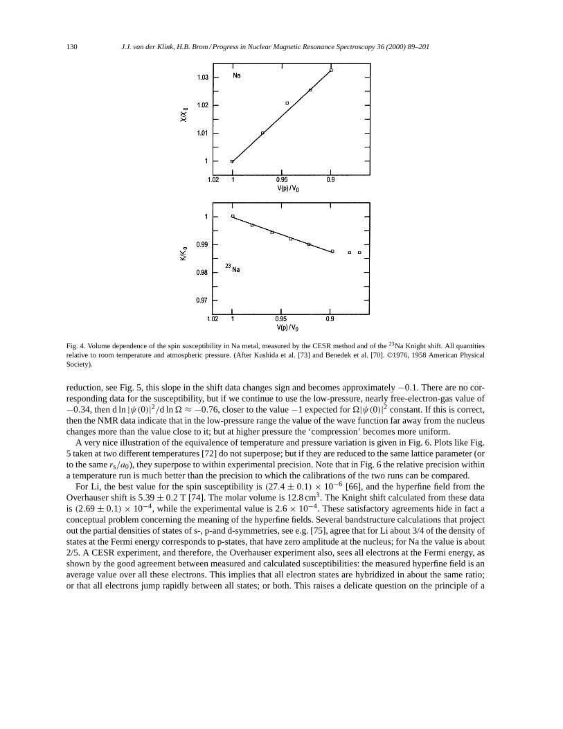
130 J.J. van der Klink, H.B. Brom / Progress in Nuclear Magnetic Resonance Spectroscopy 36 (2000) 89–201
Fig. 4. Volume dependence of the spin susceptibility in Na metal, measured by the CESR method and of the23Na Knight shift. All quantitiesrelative to room temperature and atmospheric pressure. (After Kushida et al. [73] and Benedek et al. [70]. ©1976, 1958 American PhysicalSociety).
reduction, see Fig. 5, this slope in the shift data changes sign and becomes approximately−0.1. There are no cor-responding data for the susceptibility, but if we continue to use the low-pressure, nearly free-electron-gas value of−0.34, then d ln|ψ(0)|2/d ln� ≈ −0.76, closer to the value−1 expected for�|ψ(0)|2 constant. If this is correct,then the NMR data indicate that in the low-pressure range the value of the wave function far away from the nucleuschanges more than the value close to it; but at higher pressure the ‘compression’ becomes more uniform.
A very nice illustration of the equivalence of temperature and pressure variation is given in Fig. 6. Plots like Fig.5 taken at two different temperatures [72] do not superpose; but if they are reduced to the same lattice parameter (orto the samers/a0), they superpose to within experimental precision. Note that in Fig. 6 the relative precision withina temperature run is much better than the precision to which the calibrations of the two runs can be compared.
For Li, the best value for the spin susceptibility is(27.4± 0.1) × 10−6 [66], and the hyperfine field from theOverhauser shift is 5.39± 0.2 T [74]. The molar volume is 12.8 cm3. The Knight shift calculated from these datais (2.69± 0.1) × 10−4, while the experimental value is 2.6× 10⁻⁴. These satisfactory agreements hide in fact aconceptual problem concerning the meaning of the hyperfine fields. Several bandstructure calculations that projectout the partial densities of states of s-, p-and d-symmetries, see e.g. [75], agree that for Li about 3/4 of the density ofstates at the Fermi energy corresponds to p-states, that have zero amplitude at the nucleus; for Na the value is about2/5. A CESR experiment, and therefore, the Overhauser experiment also, sees all electrons at the Fermi energy, asshown by the good agreement between measured and calculated susceptibilities: the measured hyperfine field is anaverage value over all these electrons. This implies that all electron states are hybridized in about the same ratio;or that all electrons jump rapidly between all states; or both. This raises a delicate question on the principle of a
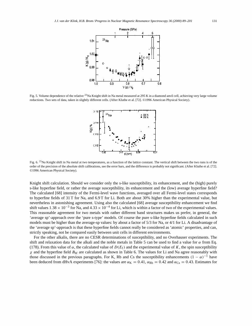
J.J. van der Klink, H.B. Brom / Progress in Nuclear Magnetic Resonance Spectroscopy 36 (2000) 89–201 131
Fig. 5. Volume dependence of the relative23Na Knight shift in Na metal measured at 295 K in a diamond anvil cell, achieving very large volumereductions. Two sets of data, taken in slightly different cells. (After Kluthe et al. [72]. ©1996 American Physical Society).
Fig. 6.23Na Knight shift in Na metal at two temperatures, as a function of the lattice constant. The vertical shift between the two runs is of theorder of the precision of the absolute shift calibrations, see the error bars, and the difference is probably not significant. (After Kluthe et al. [72].©1996 American Physical Society).
Knight shift calculation. Should we consider only the s-like susceptibility, its enhancement, and the (high) purelys-like hyperfine field, or rather the average susceptibility, its enhancement and the (low) average hyperfine field?The calculated [68] intensity of the Fermi-level wave functions, averaged over all Fermi-level states correspondsto hyperfine fields of 31 T for Na, and 6.9 T for Li. Both are about 30% higher than the experimental value, butnevertheless in astonishing agreement. Using also the calculated [68] average susceptibility enhancement we findshift values 1.38× 10⁻³ for Na, and 4.33× 10⁻⁴ for Li, which is within a factor of two of the experimental values.This reasonable agreement for two metals with rather different band structures makes us prefer, in general, the‘average sp’-approach over the ‘pure s-type’ models. Of course the pure s-like hyperfine fields calculated in suchmodels must be higher than the average-sp values: by about a factor of 5/3 for Na, or 4/1 for Li. A disadvantage ofthe ‘average sp’-approach is that these hyperfine fields cannot really be considered as ‘atomic’ properties, and can,strictly speaking, not be compared easily between unit cells in different environments.
For the other alkalis, there are no CESR determinations of susceptibility, and no Overhauser experiments. Theshift and relaxation data for the alkali and the noble metals in Table 5 can be used to find a value forα from Eq.(178). From this value ofα, the calculated value ofD(Ef ) and the experimental value ofK, the spin susceptibilityχ and the hyperfine fieldBhf are calculated as shown in Table 6. The values for Li and Na agree reasonably withthose discussed in the previous paragraphs. For K, Rb and Cs the susceptibility enhancements(1 − α)−1 havebeen deduced from dHvA experiments [76]: the values areαK = 0.41,αRb = 0.42 andαCs= 0.43. Estimates for
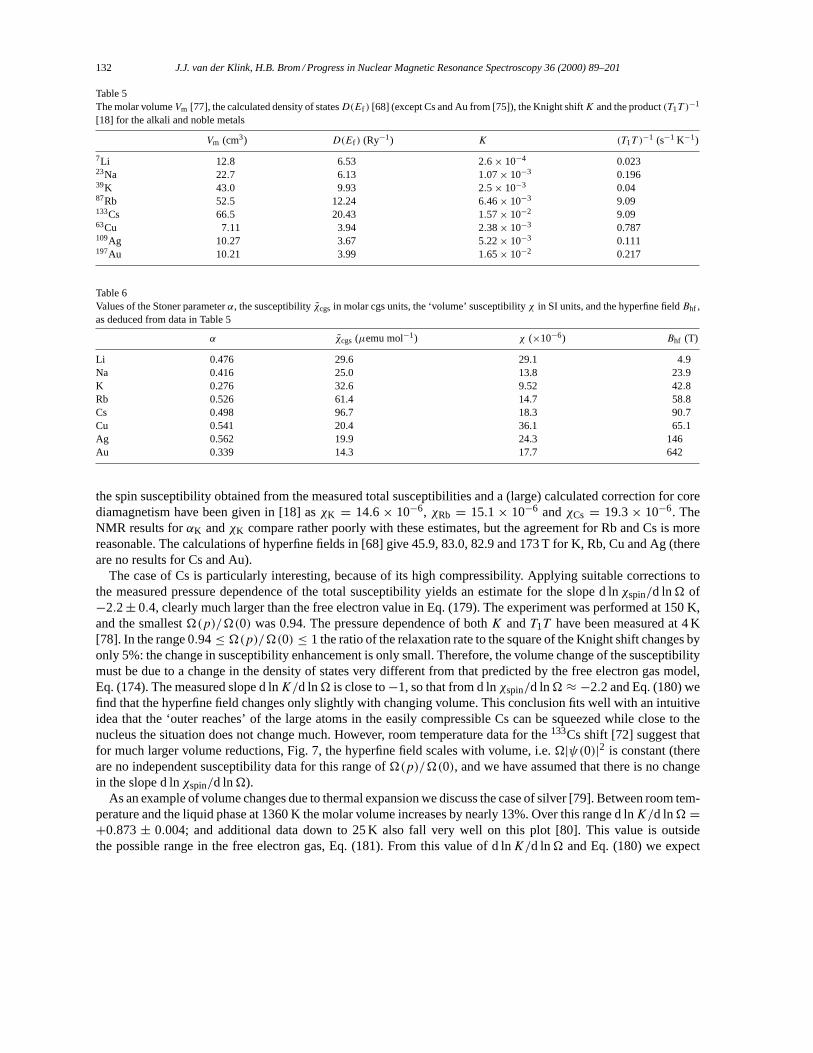
132 J.J. van der Klink, H.B. Brom / Progress in Nuclear Magnetic Resonance Spectroscopy 36 (2000) 89–201
Table 5The molar volumeVm [77], the calculated density of statesD(Ef ) [68] (except Cs and Au from [75]), the Knight shiftK and the product(T1T )
−1
[18] for the alkali and noble metals
Vm (cm3) D(Ef ) (Ry−1) K (T1T )−1 (s−1 K−1)
7Li 12.8 6.53 2.6× 10⁻⁴ 0.02323Na 22.7 6.13 1.07× 10⁻³ 0.19639K 43.0 9.93 2.5× 10⁻³ 0.0487Rb 52.5 12.24 6.46× 10⁻³ 9.09133Cs 66.5 20.43 1.57× 10⁻² 9.0963Cu 7.11 3.94 2.38× 10⁻³ 0.787109Ag 10.27 3.67 5.22× 10⁻³ 0.111197Au 10.21 3.99 1.65× 10⁻² 0.217
Table 6Values of the Stoner parameterα, the susceptibilityχcgs in molar cgs units, the ‘volume’ susceptibilityχ in SI units, and the hyperfine fieldBhf ,as deduced from data in Table 5
α χcgs (µemu mol−1) χ (×10−6) Bhf (T)
Li 0.476 29.6 29.1 4.9Na 0.416 25.0 13.8 23.9K 0.276 32.6 9.52 42.8Rb 0.526 61.4 14.7 58.8Cs 0.498 96.7 18.3 90.7Cu 0.541 20.4 36.1 65.1Ag 0.562 19.9 24.3 146Au 0.339 14.3 17.7 642
the spin susceptibility obtained from the measured total susceptibilities and a (large) calculated correction for corediamagnetism have been given in [18] asχK = 14.6× 10⁻⁶, χRb = 15.1× 10⁻⁶ andχCs = 19.3× 10⁻⁶. TheNMR results forαK andχK compare rather poorly with these estimates, but the agreement for Rb and Cs is morereasonable. The calculations of hyperfine fields in [68] give 45.9, 83.0, 82.9 and 173 T for K, Rb, Cu and Ag (thereare no results for Cs and Au).
The case of Cs is particularly interesting, because of its high compressibility. Applying suitable corrections tothe measured pressure dependence of the total susceptibility yields an estimate for the slope d lnχspin/d ln� of−2.2± 0.4, clearly much larger than the free electron value in Eq. (179). The experiment was performed at 150 K,and the smallest�(p)/�(0) was 0.94. The pressure dependence of bothK andT1T have been measured at 4 K[78]. In the range 0.94≤ �(p)/�(0) ≤ 1 the ratio of the relaxation rate to the square of the Knight shift changes byonly 5%: the change in susceptibility enhancement is only small. Therefore, the volume change of the susceptibilitymust be due to a change in the density of states very different from that predicted by the free electron gas model,Eq. (174). The measured slope d lnK/d ln� is close to−1, so that from d lnχspin/d ln� ≈ −2.2 and Eq. (180) wefind that the hyperfine field changes only slightly with changing volume. This conclusion fits well with an intuitiveidea that the ‘outer reaches’ of the large atoms in the easily compressible Cs can be squeezed while close to thenucleus the situation does not change much. However, room temperature data for the133Cs shift [72] suggest thatfor much larger volume reductions, Fig. 7, the hyperfine field scales with volume, i.e.�|ψ(0)|2 is constant (thereare no independent susceptibility data for this range of�(p)/�(0), and we have assumed that there is no changein the slope d lnχspin/d ln�).
As an example of volume changes due to thermal expansion we discuss the case of silver [79]. Between room tem-perature and the liquid phase at 1360 K the molar volume increases by nearly 13%. Over this range d lnK/d ln� =+0.873± 0.004; and additional data down to 25 K also fall very well on this plot [80]. This value is outsidethe possible range in the free electron gas, Eq. (181). From this value of d lnK/d ln� and Eq. (180) we expect
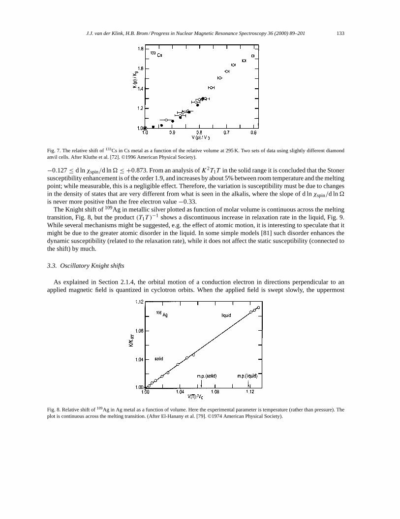
J.J. van der Klink, H.B. Brom / Progress in Nuclear Magnetic Resonance Spectroscopy 36 (2000) 89–201 133
Fig. 7. The relative shift of133Cs in Cs metal as a function of the relative volume at 295 K. Two sets of data using slightly different diamondanvil cells. After Kluthe et al. [72]. ©1996 American Physical Society).
−0.127≤ d lnχspin/d ln� ≤ +0.873. From an analysis ofK2T1T in the solid range it is concluded that the Stonersusceptibility enhancement is of the order 1.9, and increases by about 5% between room temperature and the meltingpoint; while measurable, this is a negligible effect. Therefore, the variation is susceptibility must be due to changesin the density of states that are very different from what is seen in the alkalis, where the slope of d lnχspin/d ln�is never more positive than the free electron value−0.33.
The Knight shift of109Ag in metallic silver plotted as function of molar volume is continuous across the meltingtransition, Fig. 8, but the product(T1T )
−1 shows a discontinuous increase in relaxation rate in the liquid, Fig. 9.While several mechanisms might be suggested, e.g. the effect of atomic motion, it is interesting to speculate that itmight be due to the greater atomic disorder in the liquid. In some simple models [81] such disorder enhances thedynamic susceptibility (related to the relaxation rate), while it does not affect the static susceptibility (connected tothe shift) by much.
3.3. Oscillatory Knight shifts
As explained in Section 2.1.4, the orbital motion of a conduction electron in directions perpendicular to anapplied magnetic field is quantized in cyclotron orbits. When the applied field is swept slowly, the uppermost
Fig. 8. Relative shift of109Ag in Ag metal as a function of volume. Here the experimental parameter is temperature (rather than pressure). Theplot is continuous across the melting transition. (After El-Hanany et al. [79]. ©1974 American Physical Society).
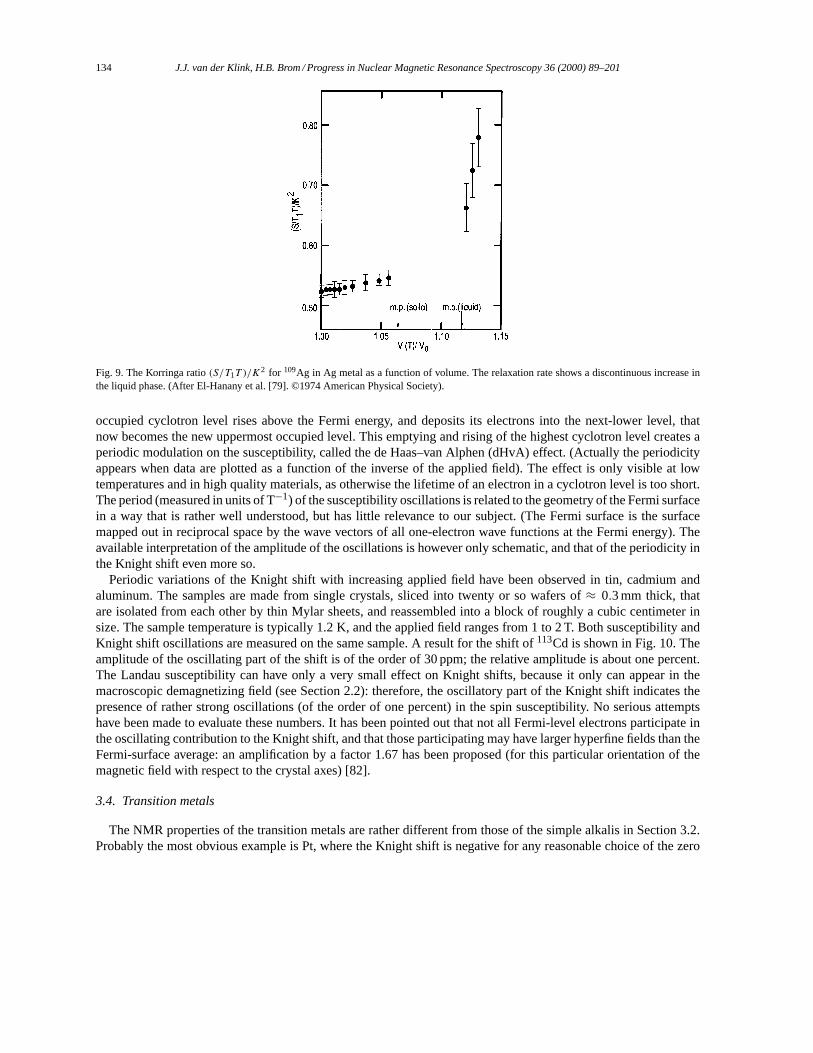
134 J.J. van der Klink, H.B. Brom / Progress in Nuclear Magnetic Resonance Spectroscopy 36 (2000) 89–201
Fig. 9. The Korringa ratio(S/T1T )/K2 for 109Ag in Ag metal as a function of volume. The relaxation rate shows a discontinuous increase in
the liquid phase. (After El-Hanany et al. [79]. ©1974 American Physical Society).
occupied cyclotron level rises above the Fermi energy, and deposits its electrons into the next-lower level, thatnow becomes the new uppermost occupied level. This emptying and rising of the highest cyclotron level creates aperiodic modulation on the susceptibility, called the de Haas–van Alphen (dHvA) effect. (Actually the periodicityappears when data are plotted as a function of the inverse of the applied field). The effect is only visible at lowtemperatures and in high quality materials, as otherwise the lifetime of an electron in a cyclotron level is too short.The period (measured in units of T−1) of the susceptibility oscillations is related to the geometry of the Fermi surfacein a way that is rather well understood, but has little relevance to our subject. (The Fermi surface is the surfacemapped out in reciprocal space by the wave vectors of all one-electron wave functions at the Fermi energy). Theavailable interpretation of the amplitude of the oscillations is however only schematic, and that of the periodicity inthe Knight shift even more so.
Periodic variations of the Knight shift with increasing applied field have been observed in tin, cadmium andaluminum. The samples are made from single crystals, sliced into twenty or so wafers of≈ 0.3 mm thick, thatare isolated from each other by thin Mylar sheets, and reassembled into a block of roughly a cubic centimeter insize. The sample temperature is typically 1.2 K, and the applied field ranges from 1 to 2 T. Both susceptibility andKnight shift oscillations are measured on the same sample. A result for the shift of113Cd is shown in Fig. 10. Theamplitude of the oscillating part of the shift is of the order of 30 ppm; the relative amplitude is about one percent.The Landau susceptibility can have only a very small effect on Knight shifts, because it only can appear in themacroscopic demagnetizing field (see Section 2.2): therefore, the oscillatory part of the Knight shift indicates thepresence of rather strong oscillations (of the order of one percent) in the spin susceptibility. No serious attemptshave been made to evaluate these numbers. It has been pointed out that not all Fermi-level electrons participate inthe oscillating contribution to the Knight shift, and that those participating may have larger hyperfine fields than theFermi-surface average: an amplification by a factor 1.67 has been proposed (for this particular orientation of themagnetic field with respect to the crystal axes) [82].
3.4. Transition metals
The NMR properties of the transition metals are rather different from those of the simple alkalis in Section 3.2.Probably the most obvious example is Pt, where the Knight shift is negative for any reasonable choice of the zero
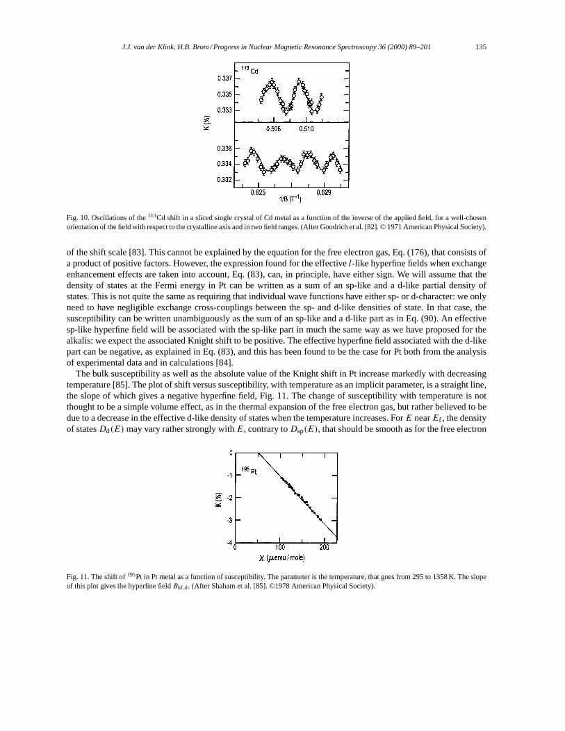
J.J. van der Klink, H.B. Brom / Progress in Nuclear Magnetic Resonance Spectroscopy 36 (2000) 89–201 135
Fig. 10. Oscillations of the113Cd shift in a sliced single crystal of Cd metal as a function of the inverse of the applied field, for a well-chosenorientation of the field with respect to the crystalline axis and in two field ranges. (After Goodrich et al. [82]. © 1971 American Physical Society).
of the shift scale [83]. This cannot be explained by the equation for the free electron gas, Eq. (176), that consists ofa product of positive factors. However, the expression found for the effectivel-like hyperfine fields when exchangeenhancement effects are taken into account, Eq. (83), can, in principle, have either sign. We will assume that thedensity of states at the Fermi energy in Pt can be written as a sum of an sp-like and a d-like partial density ofstates. This is not quite the same as requiring that individual wave functions have either sp- or d-character: we onlyneed to have negligible exchange cross-couplings between the sp- and d-like densities of state. In that case, thesusceptibility can be written unambiguously as the sum of an sp-like and a d-like part as in Eq. (90). An effectivesp-like hyperfine field will be associated with the sp-like part in much the same way as we have proposed for thealkalis: we expect the associated Knight shift to be positive. The effective hyperfine field associated with the d-likepart can be negative, as explained in Eq. (83), and this has been found to be the case for Pt both from the analysisof experimental data and in calculations [84].
The bulk susceptibility as well as the absolute value of the Knight shift in Pt increase markedly with decreasingtemperature [85]. The plot of shift versus susceptibility, with temperature as an implicit parameter, is a straight line,the slope of which gives a negative hyperfine field, Fig. 11. The change of susceptibility with temperature is notthought to be a simple volume effect, as in the thermal expansion of the free electron gas, but rather believed to bedue to a decrease in the effective d-like density of states when the temperature increases. ForE nearEf , the densityof statesDd(E)may vary rather strongly withE, contrary toDsp(E), that should be smooth as for the free electron
Fig. 11. The shift of195Pt in Pt metal as a function of susceptibility. The parameter is the temperature, that goes from 295 to 1358 K. The slopeof this plot gives the hyperfine fieldBhf,d. (After Shaham et al. [85]. ©1978 American Physical Society).
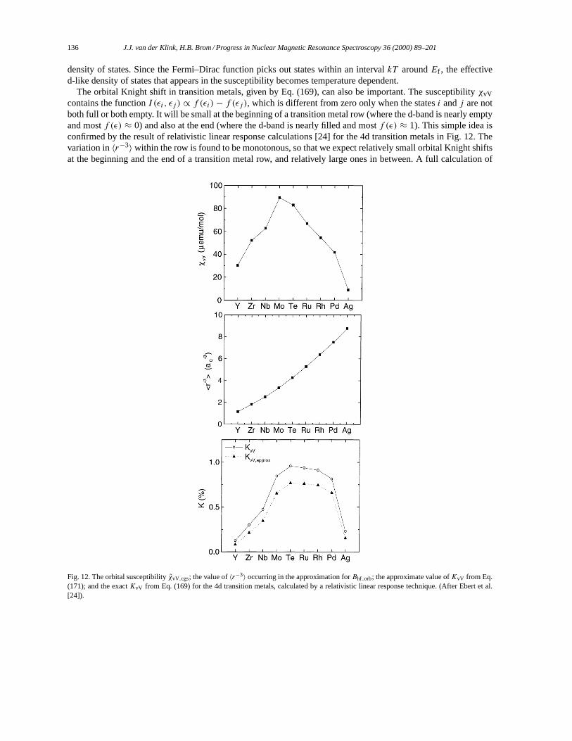
136 J.J. van der Klink, H.B. Brom / Progress in Nuclear Magnetic Resonance Spectroscopy 36 (2000) 89–201
density of states. Since the Fermi–Dirac function picks out states within an intervalkT aroundEf , the effectived-like density of states that appears in the susceptibility becomes temperature dependent.
The orbital Knight shift in transition metals, given by Eq. (169), can also be important. The susceptibilityχvVcontains the functionI (εi, εj ) ∝ f (εi)− f (εj ), which is different from zero only when the statesi andj are notboth full or both empty. It will be small at the beginning of a transition metal row (where the d-band is nearly emptyand mostf (ε) ≈ 0) and also at the end (where the d-band is nearly filled and mostf (ε) ≈ 1). This simple idea isconfirmed by the result of relativistic linear response calculations [24] for the 4d transition metals in Fig. 12. Thevariation in〈r−3〉 within the row is found to be monotonous, so that we expect relatively small orbital Knight shiftsat the beginning and the end of a transition metal row, and relatively large ones in between. A full calculation of
Fig. 12. The orbital susceptibilityχvV,cgs; the value of〈r−3〉 occurring in the approximation forBhf,orb; the approximate value ofKvV from Eq.(171); and the exactKvV from Eq. (169) for the 4d transition metals, calculated by a relativistic linear response technique. (After Ebert et al.[24]).
J.J. van der Klink, H.B. Brom / Progress in Nuclear Magnetic Resonance Spectroscopy 36 (2000) 89–201 137
KvV confirms this idea, although the exact values in Fig. 12 are up to 20% higher than those obtained using Eq.(171).
While the shift may contain positive as well as negative contributions, the relaxation rate is always a sum ofpositive terms. In the theoretical section we have shown terms proportional to the squares of the sp-like and d-likeKnight shifts introduced above in Eq. (86). There are two other contributions, that we have not discussed [44]. Ina cubic metal, the shift due to spin–dipolar coupling (Eq. (39)) is zero because of symmetry, but the fluctuatingpart contributes to the relaxation. Furthermore, the fluctuating part of the van Vleck interaction (Eq. (171)) likewisegives relaxation. These relaxation rates have only been discussed in the tight-binding approximation, where bothare found to be proportional to(Dd(Ef )Bhf,orb)
2. Strictly speaking, the hyperfine fieldBhf,orb that appears in therelaxation equations is different from that appearing in Eq. (173), but it is usual to neglect this difference. Thedipolar relaxation rate is nearly always much smaller than the orbital rate, and therefore neglected.
A refinement can be made to the relaxation equations given in the theoretical section. In Eq. (86) we have writtensums overm, wherem runs from−l to +l. In cubic metals the five values ofm corresponding tol = 2 cometogether in a triplet t2g and a doublet eg. So instead of
Dd(Ef ) =2∑
m=−2
D2m(Ef ) (182)
we should write
Dd(Ef ) = Dt2g(Ef )+Deg(Ef ) (183)
and similarly for the sum of squares
2∑m=−2
D22m(Ef ) = 3
(Dt2g(Ef )
3
)2
+ 2
(Deg(Ef )
2
)2
= RdD2d(Ef ), (184)
where the last equality defines the ‘orbital reduction factor’Rd. There is a similar, but slightly differently defined,reduction factorRorb that appears in the expression for the orbital relaxation rate. We will not go into the details ofits derivation [44], but mention for reference
Rd =2D2
t2g+ 3D2
eg
6D2d
(185)
Rorb =2Dt2g(Dt2g + 6Deg)
9D2d
. (186)
In the above paragraphs we have already introduced several approximations in the description of the shift andrelaxation rates in transition metals, the most severe being the introduction of the three densities of statesDsp(Ef ),Dt2g(Ef ) andDeg(Ef ). The advantage is that these values can be supplied by band structure calculations, and thatthe d-like hyperfine field can, sometimes, be found from experiment, as in Fig. 11. We have no reliable means tocalculate the effective Stoner factorsαl that appear in Eq. (81) and the desenhancement factorskl in the expression forthe relaxation rate, Eq. (87), are also unknown. We will suppose thatkl can be calculated from somel-independentfunction of the Stoner parameterk(α), thuskl = k(αl). A few models exist to derive the relationk(α), all ofthem for simple metals [37,69,86,87]. For want of something better they have sometimes been applied to transitionmetals as well [85,88,89,90]. Here we will adopt the Shaw–Warren result [69], which can be represented as a simplepolynomial inα, k(α) ≈ (1− α)(1+ α/4). There is little fundamental justification for doing so, but it leads to asatisfactory description of e.g. the data for Pt and for Pd. Finally, we will analyze the data in terms of the equations
138 J.J. van der Klink, H.B. Brom / Progress in Nuclear Magnetic Resonance Spectroscopy 36 (2000) 89–201
Table 7Fitted values of partial contributions to the susceptibility, the Knight shift and the relaxation rate of195Pt in platinum metal. The next four rowsgive the parameters used: hyperfine fieldsBhf , reduction factorsR, Stoner parametersα and densities of statesD(Ef ). Vm = 9.10 cm3
s d vV Total Exp.
χ(×10−6) 22.2 289 13.8 242 242K(×10−3) 7.8 −44.2 2.0 −34.4 −34.4(T1T )
−1 (s−1K−1) 7.2 19.9 6.35 33.4 33.4Bhf (T) 270 −118 110R 0.21 0.87α 0.4 0.77D(Ef ) (Ry−1) 4.08 20.4
χ ′ = µ0µ2B�−1(Dsp(Ef )
1− αsp+ Dd(Ef )
1− αd
)+ χvV = χ ′sp+ χ ′d + χvV (187)
K =(χ ′spBhf,sp+ χ ′dBhf,d + χvVBhf,orb
) �
µ0µB= Ksp+Kd +KvV (188)
S(T1T )−1 = k(αsp)K
2sp+ k(αd)K
2dRd + (µBDdBhf,orb)
2Rorb (189)
k(α) = (1− α)(1+ α
4
). (190)
In the expression for the susceptibility a diamagnetic contributionχdia has been left out. As explained in thetheoretical section, the diamagnetism of the conduction electrons only shows up as part of the demagnetizing fieldassociated withχ ′, leading to shifts of the order of a few tens of ppm (the numerical value of the diamagneticsusceptibility). For a derivation of the last term in the expression for the relaxation rate, Eq. (189), see [44].
The experimental, calculated and fitted data for Pt are shown in Table 7. The values forBhf,s = 270 T,αs =0.40 andαd = 0.77 have simply been fitted. The orbital susceptibility and hyperfine field can be estimated fromother data. The estimated diamagnetic contribution is not included in the value quoted for the total susceptibility.The d-like hyperfine fieldBhf,d = −118 T is given by the shift versus susceptibility plot. The densities of statesDs(Ef ) = 4.08 Ry−1 andDd(Ef ) = 20.4 Ry−1 [91] as well as the reduction factors [75]Rorb = 0.87 andRd = 0.21are from bandstructure calculations. The analysis of the195Pt shifts is based on the reference value195γ /2π =9.094 MHz T−1 given in the Knight shift compilation of Carter, Bennett and Kahan [18]. This was thought to givethe resonance condition for H2PtI6, but more recent values [59] put this resonance at 9.0973 MHz T−1.
There is a large uncertainty in the reference frequency for105Pd. Its NMR has been reported in only one nonmetallicsystem, two aqueous solutions of hexachloropalladate [92], with an average ratio of frequency to field ofν/B =1.9525 MHz T−1. As we have seen in Section 3.1.2, the zero of the Knight shift scale must be at smallerν/B thanany resonance in such octahedral complexes. At 4 K, the average of the values ofν/B for the metal given in [93,94]is 1.8700 MHz T−1. It follows that the Knight shiftK is more positive than−4.2×10⁻². The hexachloro complexesof Rh and Pt, neighbors of Pd in the periodic table, are at+1.5% and+0.67%, respectively, with respect to the (notvery precise) zeroes in Fig. 3, so the Knight shift of Pd is probably between−2.7×10⁻² and−3.5×10⁻². From theshift-susceptibility correlation plot the low-temperature value ofχd = 1.06×10⁻³, and ofKd = −0.0450 [94]; anearlier report [93] hasχd = 1.01×10⁻³, andKd = −0.0438. The experimental value of(T1T )
−1 = 1.35 s−1K−1.Using Eq. (189), the smallest value ofKs that is compatible with these experimental results isKs = 7.4× 10⁻³,with αs = 0. The corresponding hyperfine field isBhf,s = 520 T, which is probably too large compared to the valuegiven for Pt in Table 7 (compare the trends in Table 6). If we imposeBhf,s = 200 T, and furthermore assume a 10%error margin in the relaxation rate, we can obtain the partitioning of the susceptibility, Knight shift and relaxationrate given in Table 8. The densities of states are from [91] and the reduction factors from [75]. Note the rather largeenhancement of the s-like susceptibility found this way. The valueK = −0.0344 givesγ = 1.9366 MHz T−1 as the
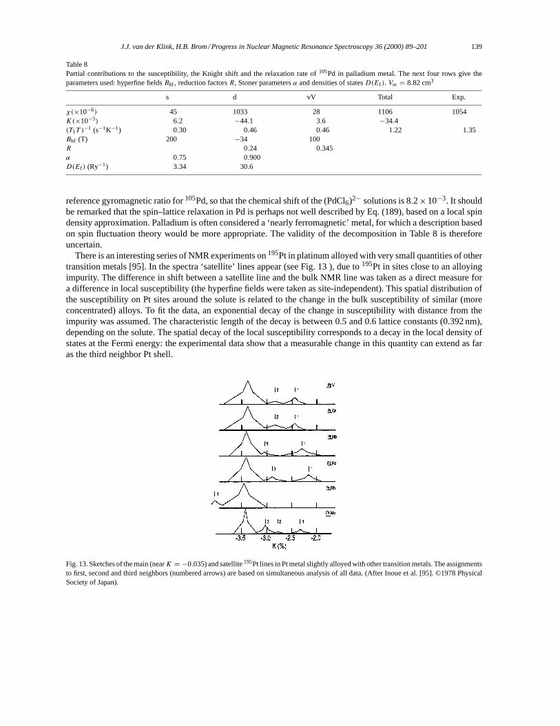
J.J. van der Klink, H.B. Brom / Progress in Nuclear Magnetic Resonance Spectroscopy 36 (2000) 89–201 139
Table 8Partial contributions to the susceptibility, the Knight shift and the relaxation rate of105Pd in palladium metal. The next four rows give theparameters used: hyperfine fieldsBhf , reduction factorsR, Stoner parametersα and densities of statesD(Ef ). Vm = 8.82 cm3
s d vV Total Exp.
χ(×10−6) 45 1033 28 1106 1054K(×10−3) 6.2 −44.1 3.6 −34.4(T1T )
−1 (s−1K−1) 0.30 0.46 0.46 1.22 1.35Bhf (T) 200 −34 100R 0.24 0.345α 0.75 0.900D(Ef ) (Ry−1) 3.34 30.6
reference gyromagnetic ratio for105Pd, so that the chemical shift of the (PdCl6)2− solutions is 8.2×10⁻³. It shouldbe remarked that the spin–lattice relaxation in Pd is perhaps not well described by Eq. (189), based on a local spindensity approximation. Palladium is often considered a ‘nearly ferromagnetic’ metal, for which a description basedon spin fluctuation theory would be more appropriate. The validity of the decomposition in Table 8 is thereforeuncertain.
There is an interesting series of NMR experiments on195Pt in platinum alloyed with very small quantities of othertransition metals [95]. In the spectra ‘satellite’ lines appear (see Fig. 13 ), due to195Pt in sites close to an alloyingimpurity. The difference in shift between a satellite line and the bulk NMR line was taken as a direct measure fora difference in local susceptibility (the hyperfine fields were taken as site-independent). This spatial distribution ofthe susceptibility on Pt sites around the solute is related to the change in the bulk susceptibility of similar (moreconcentrated) alloys. To fit the data, an exponential decay of the change in susceptibility with distance from theimpurity was assumed. The characteristic length of the decay is between 0.5 and 0.6 lattice constants (0.392 nm),depending on the solute. The spatial decay of the local susceptibility corresponds to a decay in the local density ofstates at the Fermi energy: the experimental data show that a measurable change in this quantity can extend as faras the third neighbor Pt shell.
Fig. 13. Sketches of the main (nearK = −0.035) and satellite195Pt lines in Pt metal slightly alloyed with other transition metals. The assignmentsto first, second and third neighbors (numbered arrows) are based on simultaneous analysis of all data. (After Inoue et al. [95]. ©1978 PhysicalSociety of Japan).
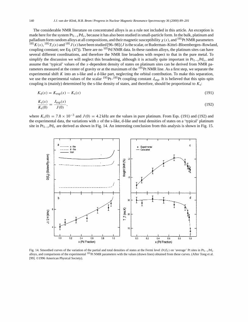
140 J.J. van der Klink, H.B. Brom / Progress in Nuclear Magnetic Resonance Spectroscopy 36 (2000) 89–201
The considerable NMR literature on concentrated alloys is as a rule not included in this article. An exception ismade here for the system Pt1−xPdx , because it has also been studied in small-particle form. In the bulk, platinum andpalladium form random alloys at all compositions, and their magnetic susceptibilityχ(x), and195Pt NMR parameters195K(x), 195T1(x)and195J (x)have been studied [96–98] (J is the scalar, or Ruderman–Kittel–Bloembergen–Rowland,coupling constant; see Eq. (47)). There are no105Pd NMR data. In these random alloys, the platinum sites can haveseveral different coordinations, and therefore the NMR line broadens with respect to that in the pure metal. Tosimplify the discussion we will neglect this broadening, although it is actually quite important in Pt1−xPdx , andassume that ‘typical’ values of thex-dependent density of states on platinum sites can be derived from NMR pa-rameters measured at the center of gravity or at the maximum of the195Pt NMR line. As a first step, we separate theexperimental shiftK into an s-like and a d-like part, neglecting the orbital contribution. To make this separation,we use the experimental values of the scalar195Pt–195Pt coupling constantJexp. It is believed that this spin–spincoupling is (mainly) determined by the s-like density of states, and therefore, should be proportional toKs:
Kd(x) = Kexp(x)−Ks(x) (191)
Ks(x)
Ks(0)= Jexp(x)
J (0), (192)
whereKs(0) = 7.8× 10⁻³ andJ (0) = 4.2 kHz are the values in pure platinum. From Eqs. (191) and (192) andthe experimental data, the variations withx of the s-like, d-like and total densities of states on a ‘typical’ platinumsite in Pt1−xPdx are derived as shown in Fig. 14. An interesting conclusion from this analysis is shown in Fig. 15.
Fig. 14. Smoothed curves of the variation of the partial and total densities of states at the Fermi levelD(Ef ) on ‘average’ Pt sites in Pt1−xPdxalloys, and comparisons of the experimental195Pt NMR parameters with the values (drawn lines) obtained from these curves. (After Tong et al.[99]. ©1996 American Physical Society).
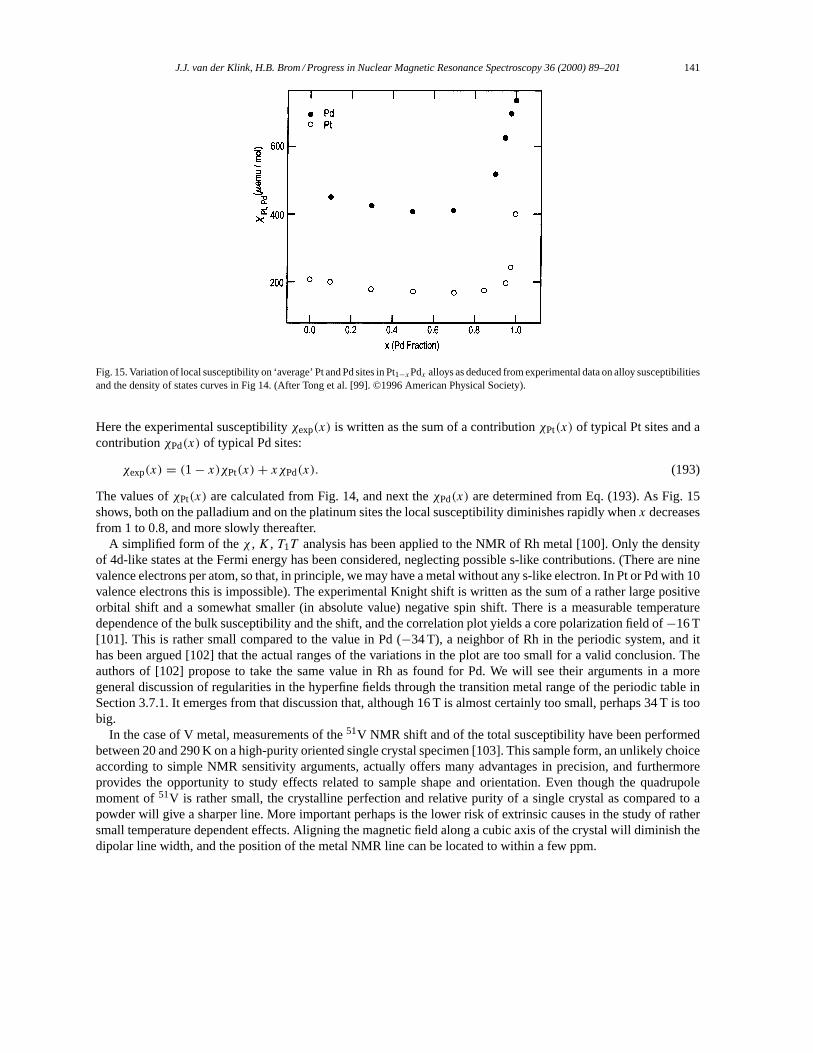
J.J. van der Klink, H.B. Brom / Progress in Nuclear Magnetic Resonance Spectroscopy 36 (2000) 89–201 141
Fig. 15. Variation of local susceptibility on ‘average’ Pt and Pd sites in Pt1−xPdx alloys as deduced from experimental data on alloy susceptibilitiesand the density of states curves in Fig 14. (After Tong et al. [99]. ©1996 American Physical Society).
Here the experimental susceptibilityχexp(x) is written as the sum of a contributionχPt(x) of typical Pt sites and acontributionχPd(x) of typical Pd sites:
χexp(x) = (1− x)χPt(x)+ xχPd(x). (193)
The values ofχPt(x) are calculated from Fig. 14, and next theχPd(x) are determined from Eq. (193). As Fig. 15shows, both on the palladium and on the platinum sites the local susceptibility diminishes rapidly whenx decreasesfrom 1 to 0.8, and more slowly thereafter.
A simplified form of theχ , K, T1T analysis has been applied to the NMR of Rh metal [100]. Only the densityof 4d-like states at the Fermi energy has been considered, neglecting possible s-like contributions. (There are ninevalence electrons per atom, so that, in principle, we may have a metal without any s-like electron. In Pt or Pd with 10valence electrons this is impossible). The experimental Knight shift is written as the sum of a rather large positiveorbital shift and a somewhat smaller (in absolute value) negative spin shift. There is a measurable temperaturedependence of the bulk susceptibility and the shift, and the correlation plot yields a core polarization field of−16 T[101]. This is rather small compared to the value in Pd (−34 T), a neighbor of Rh in the periodic system, and ithas been argued [102] that the actual ranges of the variations in the plot are too small for a valid conclusion. Theauthors of [102] propose to take the same value in Rh as found for Pd. We will see their arguments in a moregeneral discussion of regularities in the hyperfine fields through the transition metal range of the periodic table inSection 3.7.1. It emerges from that discussion that, although 16 T is almost certainly too small, perhaps 34 T is toobig.
In the case of V metal, measurements of the51V NMR shift and of the total susceptibility have been performedbetween 20 and 290 K on a high-purity oriented single crystal specimen [103]. This sample form, an unlikely choiceaccording to simple NMR sensitivity arguments, actually offers many advantages in precision, and furthermoreprovides the opportunity to study effects related to sample shape and orientation. Even though the quadrupolemoment of51V is rather small, the crystalline perfection and relative purity of a single crystal as compared to apowder will give a sharper line. More important perhaps is the lower risk of extrinsic causes in the study of rathersmall temperature dependent effects. Aligning the magnetic field along a cubic axis of the crystal will diminish thedipolar line width, and the position of the metal NMR line can be located to within a few ppm.
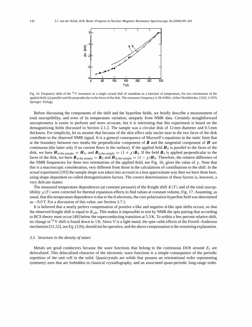
142 J.J. van der Klink, H.B. Brom / Progress in Nuclear Magnetic Resonance Spectroscopy 36 (2000) 89–201
Fig. 16. Frequency shift of the51V resonance in a single crystal disk of vanadium as a function of temperature, for two orientations of theapplied field: (a) parallel and (b) perpendicular to the faces of the disk. The resonance frequency is 38.4 MHz. (After Hechtfischer, [103]. ©1976Springer–Verlag).
Before discussing the components of the shift and the hyperfine fields, we briefly describe a measurement oftotal susceptibility, and even of its temperature variation, uniquely from NMR data. Certainly straightforwardsusceptometry is easier to perform and more accurate, but it is interesting that this experiment is based on thedemagnetizing fields discussed in Section 2.1.2. The sample was a circular disk of 12 mm diameter and 0.5 mmthickness. For simplicity, let us assume that because of the skin effect only nuclei near to the two faces of the diskcontribute to the observed NMR signal. It is a general consequence of Maxwell’s equations in the static limit thatat the boundary between two media the perpendicular component ofBBB and the tangential component ofHHH arecontinuous (the latter only if no current flows in the surface). If the applied fieldHHH 0 is parallel to the faces of thedisk, we haveHHH in the sample= HHH 0, andBBB in the sample= (1+ χ)BBB0. If the fieldBBB0 is applied perpendicular to thefaces of the disk, we haveBBB in the sample= BBB0 andHHH in the sample= (1− χ)HHH 0. Therefore, the relative difference ofthe NMR frequencies for these two orientations of the applied field, see Fig. 16, gives the value ofχ . Note thatthis is a macroscopic consideration, very different from those in the calculations of contributions to the shift. In theactual experiment [103] the sample shape was taken into account in a less approximate way then we have done here,using shape-dependent so-called demagnetization factors. The correct determination of these factors is, however, avery delicate matter.
The measured temperature dependences (at constant pressure) of the Knight shiftK(T ) and of the total suscep-tibility χ(T ) were corrected for thermal expansion effects to find values at constant volume, Fig. 17. Assuming, asusual, that this temperature dependence is due to the d-electrons, the core polarization hyperfine field was determinedas−9.0 T. For a discussion of this value, see Section 3.7.1.
It is believed that a nearly perfect compensation of positive s-like and negative d-like spin shifts occurs, so thatthe observed Knight shift is equal toKorb. This makes it impossible to test by NMR the spin pairing that accordingto BCS theory must occur [49] below the superconducting transition at 5.3 K. To within a few percent relative shift,no change in51V shift is found down to 1 K. Since V is a light metal, the spin–orbit effects of the Ferrell–Andersonmechanism [51,52], see Eq. (126), should not be operative, and the above compensation is the remaining explanation.
3.5. Structure in the density of states
Metals are good conductors because the wave functions that belong to the continuous DOS aroundEf aredelocalized. This delocalized character of the electronic wave functions is a simple consequence of the periodicrepetition of the unit cell in the solid. Quasicrystals are solids that possess an orientational order representingsymmetry axes that are forbidden in classical crystallography, and an associated quasi-periodic long-range order.
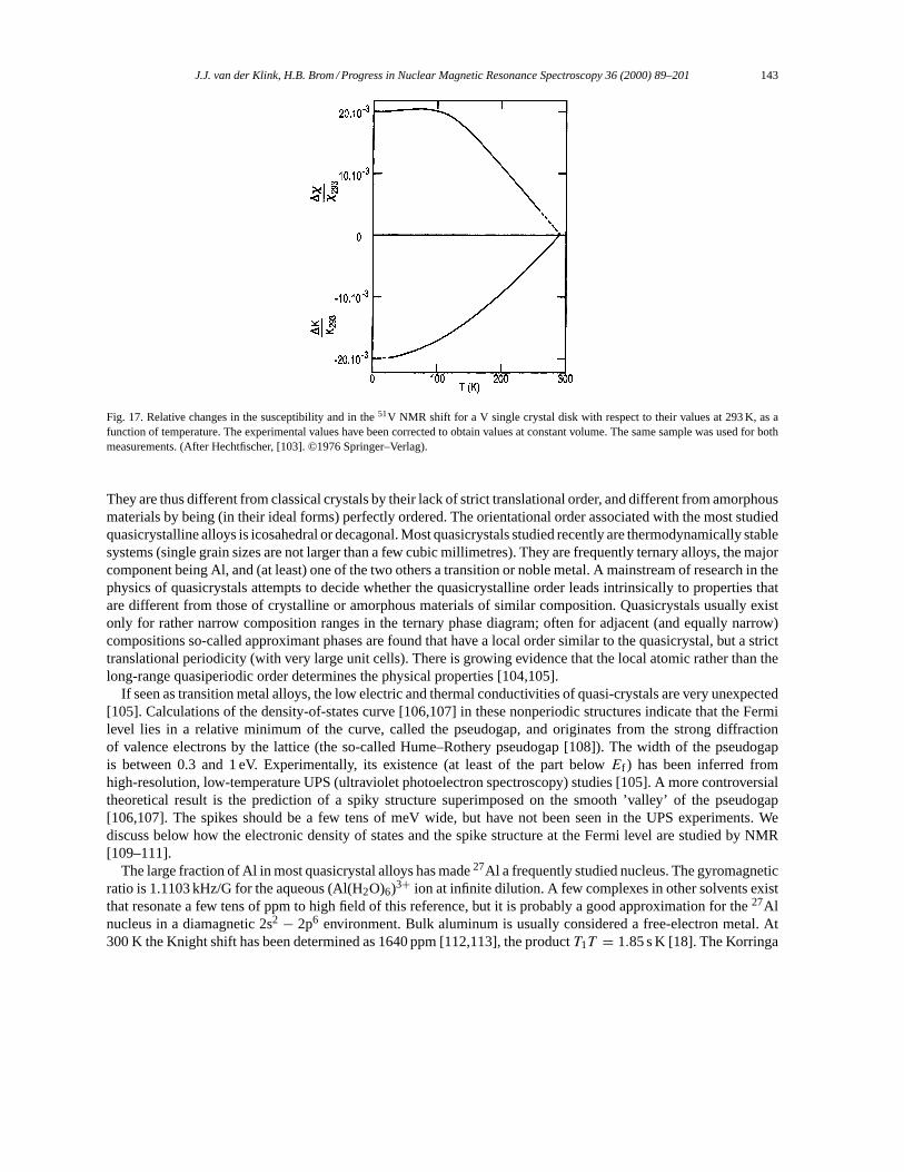
J.J. van der Klink, H.B. Brom / Progress in Nuclear Magnetic Resonance Spectroscopy 36 (2000) 89–201 143
Fig. 17. Relative changes in the susceptibility and in the51V NMR shift for a V single crystal disk with respect to their values at 293 K, as afunction of temperature. The experimental values have been corrected to obtain values at constant volume. The same sample was used for bothmeasurements. (After Hechtfischer, [103]. ©1976 Springer–Verlag).
They are thus different from classical crystals by their lack of strict translational order, and different from amorphousmaterials by being (in their ideal forms) perfectly ordered. The orientational order associated with the most studiedquasicrystalline alloys is icosahedral or decagonal. Most quasicrystals studied recently are thermodynamically stablesystems (single grain sizes are not larger than a few cubic millimetres). They are frequently ternary alloys, the majorcomponent being Al, and (at least) one of the two others a transition or noble metal. A mainstream of research in thephysics of quasicrystals attempts to decide whether the quasicrystalline order leads intrinsically to properties thatare different from those of crystalline or amorphous materials of similar composition. Quasicrystals usually existonly for rather narrow composition ranges in the ternary phase diagram; often for adjacent (and equally narrow)compositions so-called approximant phases are found that have a local order similar to the quasicrystal, but a stricttranslational periodicity (with very large unit cells). There is growing evidence that the local atomic rather than thelong-range quasiperiodic order determines the physical properties [104,105].
If seen as transition metal alloys, the low electric and thermal conductivities of quasi-crystals are very unexpected[105]. Calculations of the density-of-states curve [106,107] in these nonperiodic structures indicate that the Fermilevel lies in a relative minimum of the curve, called the pseudogap, and originates from the strong diffractionof valence electrons by the lattice (the so-called Hume–Rothery pseudogap [108]). The width of the pseudogapis between 0.3 and 1 eV. Experimentally, its existence (at least of the part belowEf ) has been inferred fromhigh-resolution, low-temperature UPS (ultraviolet photoelectron spectroscopy) studies [105]. A more controversialtheoretical result is the prediction of a spiky structure superimposed on the smooth ’valley’ of the pseudogap[106,107]. The spikes should be a few tens of meV wide, but have not been seen in the UPS experiments. Wediscuss below how the electronic density of states and the spike structure at the Fermi level are studied by NMR[109–111].
The large fraction of Al in most quasicrystal alloys has made27Al a frequently studied nucleus. The gyromagneticratio is 1.1103 kHz/G for the aqueous (Al(H2O)6)3+ ion at infinite dilution. A few complexes in other solvents existthat resonate a few tens of ppm to high field of this reference, but it is probably a good approximation for the27Alnucleus in a diamagnetic 2s2 − 2p6 environment. Bulk aluminum is usually considered a free-electron metal. At300 K the Knight shift has been determined as 1640 ppm [112,113], the productT1T = 1.85 s K [18]. The Korringa
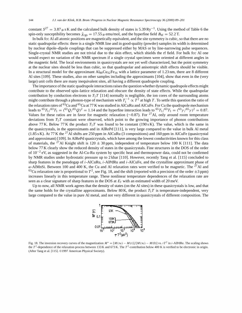
144 J.J. van der Klink, H.B. Brom / Progress in Nuclear Magnetic Resonance Spectroscopy 36 (2000) 89–201
constantS27 = 3.87m s K and the calculated bulk density of states is 5.39 Ry−1. Using the method of Table 6 thespin-only susceptibility becomesχcgs= 17.55m emu/mol, and the hyperfine fieldBhf = 52.2 T.
In bulk fcc Al all atomic positions are magnetically equivalent, and the site symmetry is cubic, so that there are nostatic quadrupolar effects: there is a single NMR line and in good-quality (powder) samples its width is determinedby nuclear dipole–dipole couplings that can be suppressed either by MAS or by line-narrowing pulse sequences.Single-crystal NMR studies are not trivial due to the skin effect, which shields the rf field. For bulk fcc Al onewould expect no variation of the NMR spectrum if a single crystal specimen were oriented at different angles inthe magnetic field. The local environments in quasicrystals are not yet well characterized, but the point symmetryat the nuclear sites should be less than cubic, so that quadrupolar and anisotropic shift effects should be visible.In a structural model for the approximant Al80Cu32Fe16 with a lattice parameter of 1.23 nm, there are 8 differentAl sites [109]. These studies, also on other samples including the approximants [104], show that even in the (verylarge) unit cells there are many inequivalent sites, all having a different quadrupole coupling.
The importance of the static quadrupole interactions raises the question whether dynamic quadrupole effects mightcontribute to the observed spin–lattice relaxation and obscure the density of state effects. While the quadrupolarcontribution by conduction electrons toT1T [114] normally is negligible, the ion cores of the surrounding atomsmight contribute through a phonon-type of mechanism withT −1
1 ∝ T 2 at highT . To settle this question the ratio ofthe relaxation rates of63Cu and65Cu at 77 K was studied in AlCuRu and AlCuFe. For Cu the quadrupole mechanismleads to65T1/
63T1 = (63Q/65Q)2 = 1.14 and the hyperfine interaction leads to65T1/63T1 = (63γ /65γ )2 = 0.87.
Values for these ratios are in favor for magnetic relaxation (∼0.87). For27Al, only around room temperaturedeviations fromT1T constant were observed, which point to the growing importance of phonon contributionsabove 77 K. Below 77 K the productT1T was found to be constant (190 s K). The value, which is the same inthe quasicrystals, in the approximants and in AlRePd [111], is very large compared to the value in bulk Al metal(1.85 s K). At 77 K the27Al shifts are 250 ppm in AlCuRu (3 compositions) and 160 ppm in AlCuFe (quasicrystaland approximant) [109]. In AlRePd quasicrystals, which have among the lowest conductivities known for this classof materials, the27Al Knight shift is 120± 30 ppm, independent of temperature below 100 K [111]. The databelow 77 K clearly show the reduced density of states in the quasicrystals. Fine structures in the DOS of the orderof 10−2 eV, as suggested in the Al-Cu-Ru system by specific heat and thermopower data, could not be confirmedby NMR studies under hydrostatic pressure up to 2 kbar [110]. However, recently Tang et al. [115] concluded tosharp features in the pseudogap ofi-AlCuRu, i-AlPdRu andi-AlCuFe, and the crystalline approximant phase ofα-AlMnSi. Between 100 and 400 K, the Cu and Al relaxation rates were verified to be magnetic. The27Al and63Cu relaxation rate is proportional toT 2, see Fig. 18, and the shift (reported with a precision of the order±3 ppm)increases linearly in this temperature range. These nonlinear temperature dependences of the relaxation rate areseen as a clear signature of sharp features in the DOS atEf with an estimated width of 20 meV.
Up to now, all NMR work agrees that the density of states (on the Al sites) in these quasicrystals is low, and thatthe same holds for the crystalline approximants. Below 80 K, the productT1T is temperature-independent, verylarge compared to the value in pure Al metal, and not very different in quasicrystals of different composition. The
Fig. 18. The inversion recovery curves of the magnetizationM∗ = [M(∞)−M(t)]/[M(∞)−M(0)] vs. tT 2 in i-AlPdRe. The scaling showstheT 2-dependence of the relaxation process between 133 K and 673 K. TheT 2-contribution below 400 K is verified to be electronic in origin.(After Tang et al. [115]. ©1997 American Physical Society).
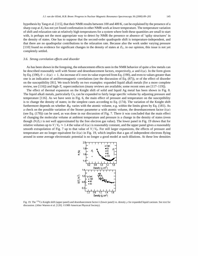
J.J. van der Klink, H.B. Brom / Progress in Nuclear Magnetic Resonance Spectroscopy 36 (2000) 89–201 145
hypothesis by Tang et al. [115], that their NMR results between 100 and 400 K, can be explained by the presence of asharp cusp atEf has not yet found confirmation in other NMR work at lower temperature. The temperature variationof shift and relaxation rate at relatively high temperatures for a system where both these quantities are small to startwith, is perhaps not the most appropriate way to detect by NMR the presence or absence of ’spiky structures’ inthe density of states. One has to suppose that the second-order quadrupole shift is temperature-independent, andthat there are no quadrupolar contributions to the relaxation rate. Because also the work under varying pressure[110] found no evidence for significant changes in the density of states atEf , in our opinion, this issue is not yetcompletely settled.
3.6. Strong correlation effects and disorder
As has been shown in the foregoing, the enhancement effects seen in the NMR behavior of quite a few metals canbe described reasonably well with Stoner and desenhancement factors, respectively,α andk(α). In the form givenby Eq. (190), 0< k(α) < 1. An increase ofk over its value expected from Eq. (190), and even to values greater thanone is an indication of antiferromagnetic correlations (see the discussion of Eq. (87)), or of the effect of disorderon the susceptibility [81]. We touch briefly on two examples: expanded liquid alkali metals (for a more completereview, see [116]) and high-Tc superconductors (many reviews are available; some recent ones are [117–119]).
The effect of thermal expansion on the Knight shift of solid and liquid Ag metal has been shown in Fig. 8.The liquid alkali metals, particularly Cs, can be expanded to fairly large specific volume by adjusting pressure andtemperature [116]. As we have seen in Fig. 6, the main effect of pressure and temperature on the susceptibilityis to change the density of states; in the simplest cases according to Eq. (174). The variation of the Knight shiftfurthermore depends on whetherBhf varies with the atomic volume, e.g. within the limits given by Eq. (181). Asa check on the possible variation of the Stoner parameterα with atomic volume, the desenhancement factork(α)
(see Eq. (178)) can be used, as was done in our discussion of Fig. 7. There it was concluded that the main effectof changing the molecular volume at ambient temperature and pressure is a change in the density of states (eventhoughD(Ef ) is not well approximated by the free electron gas value). The lower panel in Fig. 19 shows that forrelative volumes up toV/V0 ≈ 1.4 the value ofk(α) is reasonably constant, and the upper panel gives a reasonablysmooth extrapolation of Fig. 7 up to that value ofV/V0. For still larger expansions, the effects of pressure andtemperature are no longer equivalent fork(α) in Fig. 19, which implies that a gas of independent electrons flyingaround in some average electrostatic potential is no longer a good model at such dilutions. At these low densities
Fig. 19. The133Cs Knight shift (upper panel) and desenhancement factork (lower panel) vs. densityρ for expanded liquid caesium. See text fordiscussion. (After Warren et al. [120]. ©1989 American Physical Society).
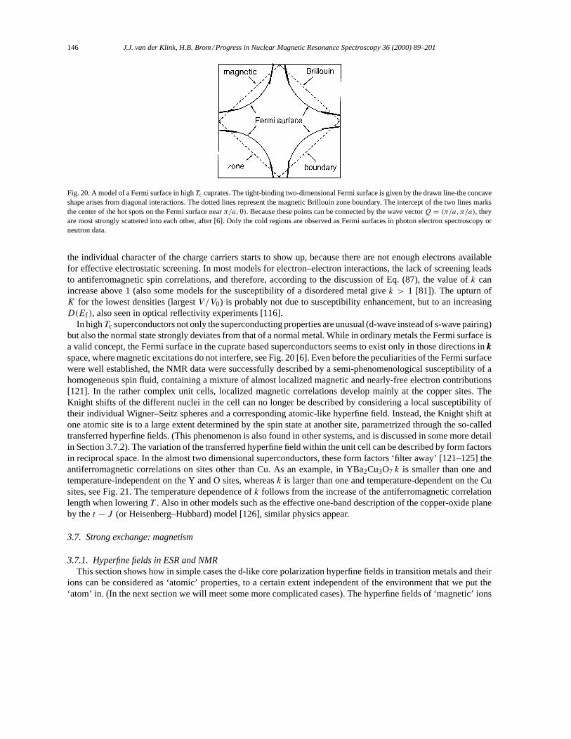
146 J.J. van der Klink, H.B. Brom / Progress in Nuclear Magnetic Resonance Spectroscopy 36 (2000) 89–201
Fig. 20. A model of a Fermi surface in highTc cuprates. The tight-binding two-dimensional Fermi surface is given by the drawn line-the concaveshape arises from diagonal interactions. The dotted lines represent the magnetic Brillouin zone boundary. The intercept of the two lines marksthe center of the hot spots on the Fermi surface nearπ/a,0). Because these points can be connected by the wave vectorQ = (π/a, π/a), theyare most strongly scattered into each other, after [6]. Only the cold regions are observed as Fermi surfaces in photon electron spectroscopy orneutron data.
the individual character of the charge carriers starts to show up, because there are not enough electrons availablefor effective electrostatic screening. In most models for electron–electron interactions, the lack of screening leadsto antiferromagnetic spin correlations, and therefore, according to the discussion of Eq. (87), the value ofk canincrease above 1 (also some models for the susceptibility of a disordered metal givek > 1 [81]). The upturn ofK for the lowest densities (largestV/V0) is probably not due to susceptibility enhancement, but to an increasingD(Ef ), also seen in optical reflectivity experiments [116].
In highTc superconductors not only the superconducting properties are unusual (d-wave instead of s-wave pairing)but also the normal state strongly deviates from that of a normal metal. While in ordinary metals the Fermi surface isa valid concept, the Fermi surface in the cuprate based superconductors seems to exist only in those directions inkkk
space, where magnetic excitations do not interfere, see Fig. 20 [6]. Even before the peculiarities of the Fermi surfacewere well established, the NMR data were successfully described by a semi-phenomenological susceptibility of ahomogeneous spin fluid, containing a mixture of almost localized magnetic and nearly-free electron contributions[121]. In the rather complex unit cells, localized magnetic correlations develop mainly at the copper sites. TheKnight shifts of the different nuclei in the cell can no longer be described by considering a local susceptibility oftheir individual Wigner–Seitz spheres and a corresponding atomic-like hyperfine field. Instead, the Knight shift atone atomic site is to a large extent determined by the spin state at another site, parametrized through the so-calledtransferred hyperfine fields. (This phenomenon is also found in other systems, and is discussed in some more detailin Section 3.7.2). The variation of the transferred hyperfine field within the unit cell can be described by form factorsin reciprocal space. In the almost two dimensional superconductors, these form factors ‘filter away’ [121–125] theantiferromagnetic correlations on sites other than Cu. As an example, in YBa2Cu3O7 k is smaller than one andtemperature-independent on the Y and O sites, whereask is larger than one and temperature-dependent on the Cusites, see Fig. 21. The temperature dependence ofk follows from the increase of the antiferromagnetic correlationlength when loweringT . Also in other models such as the effective one-band description of the copper-oxide planeby thet − J (or Heisenberg–Hubbard) model [126], similar physics appear.
3.7. Strong exchange: magnetism
3.7.1. Hyperfine fields in ESR and NMRThis section shows how in simple cases the d-like core polarization hyperfine fields in transition metals and their
ions can be considered as ‘atomic’ properties, to a certain extent independent of the environment that we put the‘atom’ in. (In the next section we will meet some more complicated cases). The hyperfine fields of ‘magnetic’ ions
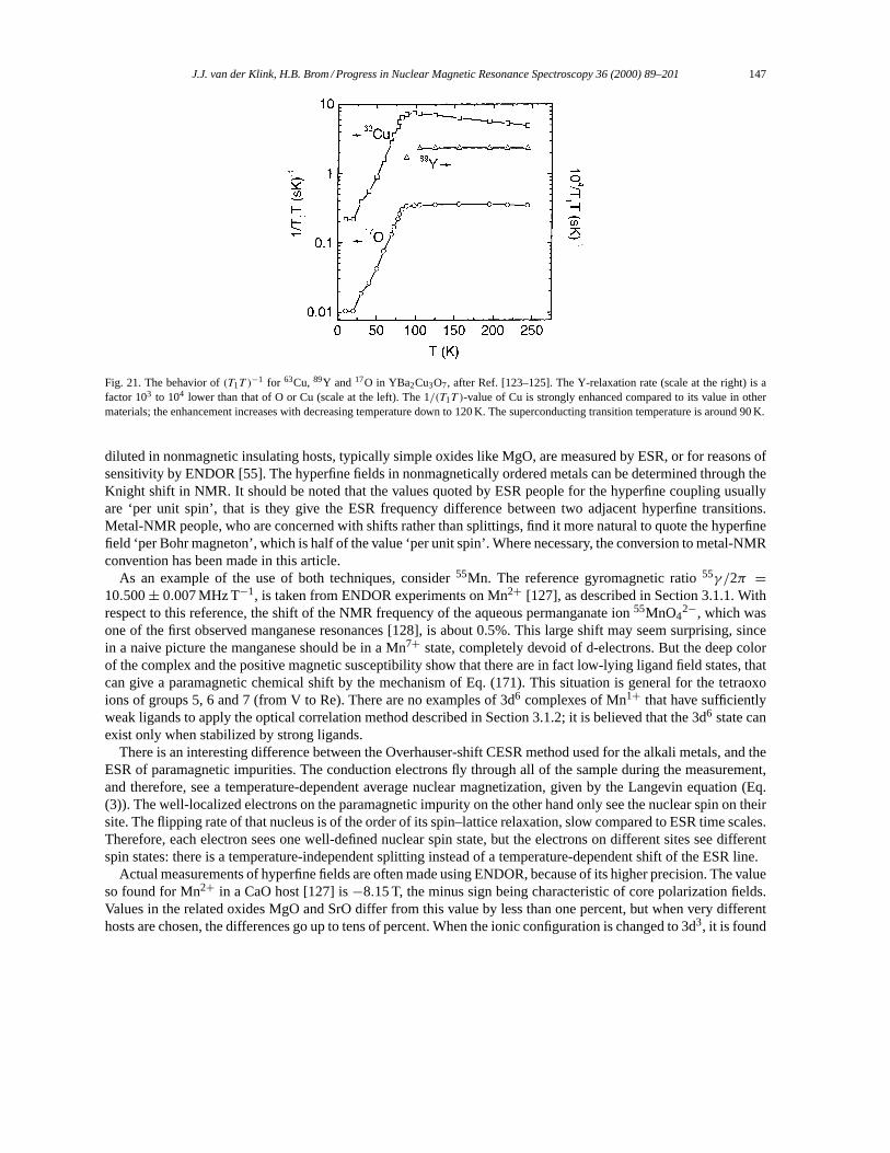
J.J. van der Klink, H.B. Brom / Progress in Nuclear Magnetic Resonance Spectroscopy 36 (2000) 89–201 147
Fig. 21. The behavior of(T1T )−1 for 63Cu, 89Y and 17O in YBa2Cu3O7, after Ref. [123–125]. The Y-relaxation rate (scale at the right) is a
factor 103 to 104 lower than that of O or Cu (scale at the left). The 1/(T1T )-value of Cu is strongly enhanced compared to its value in othermaterials; the enhancement increases with decreasing temperature down to 120 K. The superconducting transition temperature is around 90 K.
diluted in nonmagnetic insulating hosts, typically simple oxides like MgO, are measured by ESR, or for reasons ofsensitivity by ENDOR [55]. The hyperfine fields in nonmagnetically ordered metals can be determined through theKnight shift in NMR. It should be noted that the values quoted by ESR people for the hyperfine coupling usuallyare ‘per unit spin’, that is they give the ESR frequency difference between two adjacent hyperfine transitions.Metal-NMR people, who are concerned with shifts rather than splittings, find it more natural to quote the hyperfinefield ‘per Bohr magneton’, which is half of the value ‘per unit spin’. Where necessary, the conversion to metal-NMRconvention has been made in this article.
As an example of the use of both techniques, consider55Mn. The reference gyromagnetic ratio55γ /2π =10.500± 0.007 MHz T−1, is taken from ENDOR experiments on Mn2+ [127], as described in Section 3.1.1. Withrespect to this reference, the shift of the NMR frequency of the aqueous permanganate ion55MnO4
2−, which wasone of the first observed manganese resonances [128], is about 0.5%. This large shift may seem surprising, sincein a naive picture the manganese should be in a Mn7+ state, completely devoid of d-electrons. But the deep colorof the complex and the positive magnetic susceptibility show that there are in fact low-lying ligand field states, thatcan give a paramagnetic chemical shift by the mechanism of Eq. (171). This situation is general for the tetraoxoions of groups 5, 6 and 7 (from V to Re). There are no examples of 3d6 complexes of Mn1+ that have sufficientlyweak ligands to apply the optical correlation method described in Section 3.1.2; it is believed that the 3d6 state canexist only when stabilized by strong ligands.
There is an interesting difference between the Overhauser-shift CESR method used for the alkali metals, and theESR of paramagnetic impurities. The conduction electrons fly through all of the sample during the measurement,and therefore, see a temperature-dependent average nuclear magnetization, given by the Langevin equation (Eq.(3)). The well-localized electrons on the paramagnetic impurity on the other hand only see the nuclear spin on theirsite. The flipping rate of that nucleus is of the order of its spin–lattice relaxation, slow compared to ESR time scales.Therefore, each electron sees one well-defined nuclear spin state, but the electrons on different sites see differentspin states: there is a temperature-independent splitting instead of a temperature-dependent shift of the ESR line.
Actual measurements of hyperfine fields are often made using ENDOR, because of its higher precision. The valueso found for Mn2+ in a CaO host [127] is−8.15 T, the minus sign being characteristic of core polarization fields.Values in the related oxides MgO and SrO differ from this value by less than one percent, but when very differenthosts are chosen, the differences go up to tens of percent. When the ionic configuration is changed to 3d3, it is found
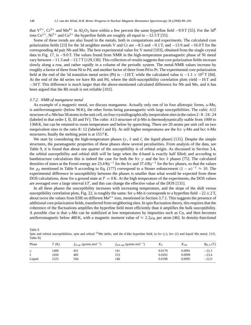
148 J.J. van der Klink, H.B. Brom / Progress in Nuclear Magnetic Resonance Spectroscopy 36 (2000) 89–201
that V2+, Cr3+ and Mn4+ in Al2O3 have within a few percent the same hyperfine field−9.9 T [55]. For the 3d8
ions Co1+, Ni2+ and Cu3+ the hyperfine fields are roughly all equal to−12.5 T [55].Some of these trends are also found in the metals, both in computations and experiments. The calculated core
polarization fields [23] for the 3d neighbor metals V and Cr are−8.5 and−9.1 T, and−13.9 and−16.0 T for thecorresponding 4d pair Nb and Mo. The best experimental value for V metal [103], obtained from the single crystaldata in Fig. 17, is−9.0 T. The values found from NMR in the high-temperature paramagnetic phase of Ni metalvary between−11.3 and−13.7 T [129,130]. This collection of results suggests that core polarization fields increaseslowly along a row, and rather rapidly in a column of the periodic system. The metal-NMR values increase byroughly a factor of three from Ni to Pd, and another factor of three from Pd to Pt. The experimental core polarizationfield at the end of the 5d transition metal series (Pt) is−118 T, while the calculated value is−1.1× 10² T [84].At the end of the 4d series we have Rh and Pd, where the shift-susceptibility correlation plots yield−16 T and−34 T. This difference is much larger than the above-mentioned calculated difference for Nb and Mo, and it hasbeen argued that the Rh result is not reliable [102].
3.7.2. NMR of manganese metalAs example of a magnetic metal, we discuss manganese. Actually only one of its four allotropic forms,a-Mn,
is antiferromagnetic (below 96 K), the other forms being paramagnetic with large susceptibilities. The cubicA12structure ofa-Mn has 58 atoms in the unit cell, on four crystallographically inequivalent sites in the ratios2 : 8 : 24 : 24(labeled in that order I, II, III and IV). The cubicA13 structure ofb-Mn is thermodynamically stable from 1000 to1368 K, but can be retained to room temperature and below by quenching. There are 20 atoms per unit cell on twoinequivalent sites in the ratio 8 : 12 (labeled I and II). At still higher temperatures are the fccg-Mn and bccd-Mnstructures; finally the melting point is at 1517 K.
We start by considering the high-temperature phases (γ , δ and`, the liquid phase) [131]. Despite the simplestructures, the paramagnetic properties of these phases show several peculiarities. From analysis of the data, seeTable 9, it is found that about one quarter of the susceptibility is of orbital origin. As discussed in Section 3.4,the orbital susceptibility and orbital shift will be large when the d-band is exactly half filled; and according tobandstructure calculations this is indeed the case for both the fccγ and the bccδ phases [75]. The calculateddensities of states at the Fermi energy are 23.4 Ry−1 for the fcc and 37.4 Ry−1 for the bcc phases, so that the valuesfor χd mentioned in Table 9 according to Eq. (177) correspond to a Stoner enhancement(1− α)−1 ≈ 10. Theexperimental difference in susceptibility between the phases is smaller than what would be expected from theseDOS calculations, done for a ground state atT = 0 K. At the high temperature of the experiments, the DOS valuesare averaged over a large intervalkT , and this can change the effective value of the DOS [131].
In all three phases the susceptibility increases with increasing temperature, and the slope of the shift versussusceptibility correlation plots, Fig. 22, is roughly the same: forg-Mn it corresponds to a hyperfine field−22±2 T,about twice the values from ESR on different Mnn+ ions, mentioned in Section 3.7.1. This suggests the presence ofadditional core polarization fields, transferred from neighboring sites. In spin fluctuation theory, this requires that thecoherence of the fluctuations amplifies the hyperfine field more efficiently than it amplifies the bulk susceptibility.A possible clue is thatg-Mn can be stabilized at low temperatures by impurities such as Cu, and then becomesantiferromagnetic below 480 K, with a magnetic moment value of≈ 2.2µB per atom [46]. In density-functional
Table 9Spin and orbital susceptibilities, spin and orbital55Mn shifts, and the d-like hyperfine field, in fcc (γ ), bcc (δ) and liquid Mn metal. [131,Table II]
Phase T (K) χd,cgs (memu mol−1) χorb,cgs (memu mol−1) Kd Korb Bhf,d (T)
γ 1400 451 141 0.0179 0.0091 −22.3δ 1450 485 153 0.0202 0.0099 −23.4Liquid 1525 504 146 0.0198 0.0095 −22.0
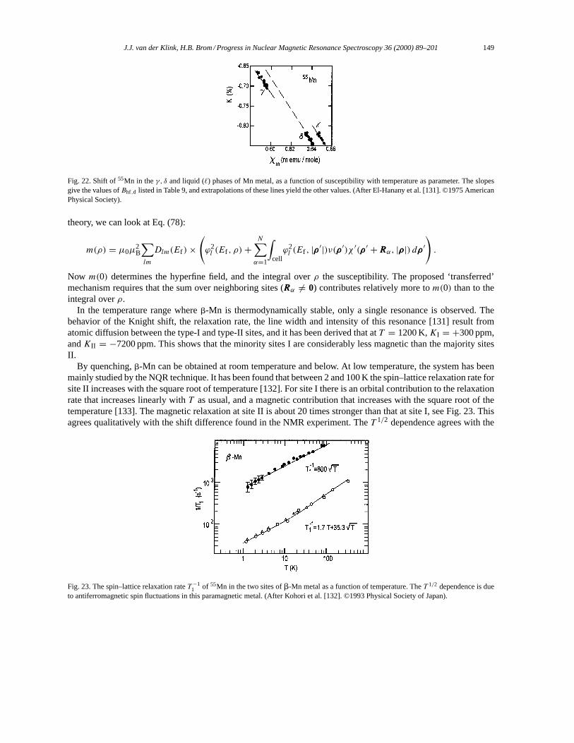
J.J. van der Klink, H.B. Brom / Progress in Nuclear Magnetic Resonance Spectroscopy 36 (2000) 89–201 149
Fig. 22. Shift of55Mn in theγ, δ and liquid ( ) phases of Mn metal, as a function of susceptibility with temperature as parameter. The slopesgive the values ofBhf,d listed in Table 9, and extrapolations of these lines yield the other values. (After El-Hanany et al. [131]. ©1975 AmericanPhysical Society).
theory, we can look at Eq. (78):
m(ρ) = µ0µ2B
∑lm
Dlm(Ef )×(ϕ2l (Ef , ρ)+
N∑α=1
∫cellϕ2l (Ef , |ρρρ′|)ν(ρρρ′)χ ′(ρρρ′ +RRRα, |ρρρ|) dρρρ′
).
Now m(0) determines the hyperfine field, and the integral overρ the susceptibility. The proposed ‘transferred’mechanism requires that the sum over neighboring sites (RRRα 6= 0) contributes relatively more tom(0) than to theintegral overρ.
In the temperature range whereb-Mn is thermodynamically stable, only a single resonance is observed. Thebehavior of the Knight shift, the relaxation rate, the line width and intensity of this resonance [131] result fromatomic diffusion between the type-I and type-II sites, and it has been derived that atT = 1200 K,KI = +300 ppm,andKII = −7200 ppm. This shows that the minority sites I are considerably less magnetic than the majority sitesII.
By quenching,b-Mn can be obtained at room temperature and below. At low temperature, the system has beenmainly studied by the NQR technique. It has been found that between 2 and 100 K the spin–lattice relaxation rate forsite II increases with the square root of temperature [132]. For site I there is an orbital contribution to the relaxationrate that increases linearly withT as usual, and a magnetic contribution that increases with the square root of thetemperature [133]. The magnetic relaxation at site II is about 20 times stronger than that at site I, see Fig. 23. Thisagrees qualitatively with the shift difference found in the NMR experiment. TheT 1/2 dependence agrees with the
Fig. 23. The spin–lattice relaxation rateT −11 of 55Mn in the two sites ofb-Mn metal as a function of temperature. TheT 1/2 dependence is due
to antiferromagnetic spin fluctuations in this paramagnetic metal. (After Kohori et al. [132]. ©1993 Physical Society of Japan).
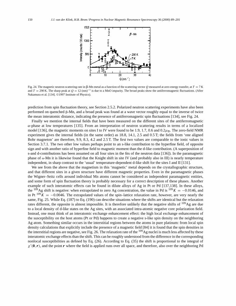
150 J.J. van der Klink, H.B. Brom / Progress in Nuclear Magnetic Resonance Spectroscopy 36 (2000) 89–201
Fig. 24. The magnetic neutron scattering rate inb-Mn metal as a function of the scattering vectorQmeasured at zero energy transfer, atT = 7 KandT = 290 K. The sharp peak atQ = 12 (nm)−1 is due to a MnO impurity. The broad peaks show the antiferromagnetic fluctuations. (AfterNakamura et al. [134]. ©1997 Institute of Physics).
prediction from spin fluctuation theory, see Section 2.5.2. Polarized neutron scattering experiments have also beenperformed on quenchedb-Mn, and a broad peak was found at a wave vector roughly equal to the inverse of twicethe mean interatomic distance, indicating the presence of antiferromagnetic spin fluctuations [134], see Fig. 24.
Finally we mention the internal fields that have been measured on the different sites of the antiferromagneticα-phase at low temperatures [135]. From an interpretation of neutron scattering results in terms of a localizedmodel [136], the magnetic moments on sites I to IV were found to be 1.9, 1.7, 0.6 and 0.2µB. The zero-field NMRexperiment gives the internal fields (in the same order) as 18.8, 14.1, 2.5 and 0.5 T; the fields from ‘one alignedBohr magneton’ are therefore, 9.9, 8.3, 4.2 and 2.5 T. The first two values are comparable to the ionic values inSection 3.7.1. The two other low values perhaps point to an s-like contribution to the hyperfine field, of oppositesign and with another ratio of hyperfine field to magnetic moment than the d-like contribution. (A superposition ofs-and d-contributions has been assumed on all four sites in the fits of the neutron data [136]). In the paramagneticphase ofa-Mn it is likewise found that the Knight shift in site IV (and probably also in III) is nearly temperatureindependent, in sharp contrast to the ‘usual’ temperature-dependent d-like shift for the sites I and II [131].
We see from the above that the magnetism in this ‘magnetic’ metal depends on the crystallographic structure,and that different sites in a given structure have different magnetic properties. Even in the paramagnetic phasesthe Wigner–Seitz cells around individual Mn atoms cannot be considered as independent paramagnetic entities,and some form of spin fluctuation theory is probably necessary for a correct description of these phases. Anotherexample of such interatomic effects can be found in dilute alloys of Ag in Pt or Pd [137,138]. In these alloys,the109Ag shift is negative: when extrapolated to zero Ag concentration, the value in Pd is109K = −0.0146, andin Pt 109K = −0.0046. The extrapolated values of the spin–lattice relaxation rate, however, are very nearly thesame, Fig. 25. While Eq. (187) to Eq. (190) can describe situations where the shifts are identical but the relaxationrates different, the opposite is almost impossible. It is therefore unlikely that the negative shifts of109Ag are dueto a local density of d-like states on the Ag sites, with an associated intra-atomic negative core polarization field.Instead, one must think of an interatomic exchange enhancement effect: the high local exchange enhancement ofthe susceptibility on the host atoms (Pt or Pd) happens to create a negative s-like spin density on the neighboringAg atom. Something similar occurs in the interstitial regions between the atoms in pure platinum: from local spindensity calculations that explicitly include the presence of a magnetic field [84] it is found that the spin densities inthe interstitial regions are negative, see Fig. 26. The relaxation rate of the109Ag nuclei is much less affected by theseinteratomic exchange effects than the shift. This can be roughly understood from the difference in the correspondingnonlocal susceptibilities as defined by Eq. (26). According to Eq. (35) the shift is proportional to the integral ofχ ′(0, rrr), and the pointrrr where the field is applied runs over all space, and therefore, also over the neighboring Pd
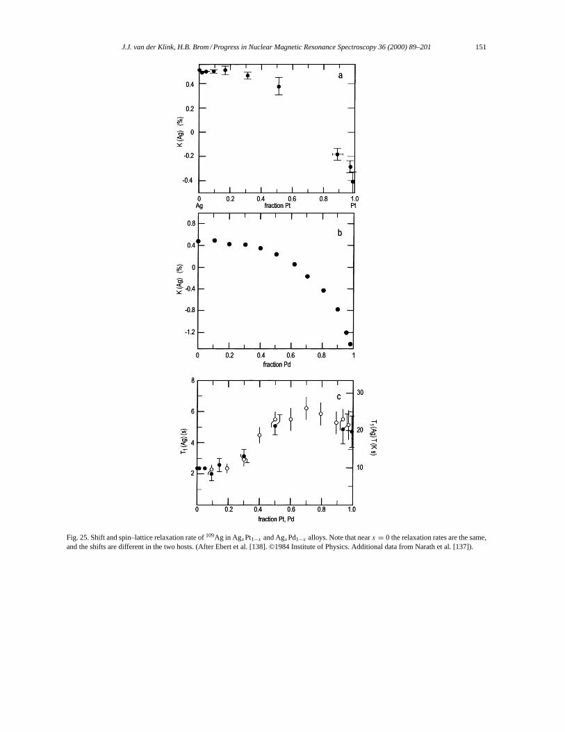
J.J. van der Klink, H.B. Brom / Progress in Nuclear Magnetic Resonance Spectroscopy 36 (2000) 89–201 151
Fig. 25. Shift and spin–lattice relaxation rate of109Ag in AgxPt1−x and AgxPd1−x alloys. Note that nearx = 0 the relaxation rates are the same,and the shifts are different in the two hosts. (After Ebert et al. [138]. ©1984 Institute of Physics. Additional data from Narath et al. [137]).
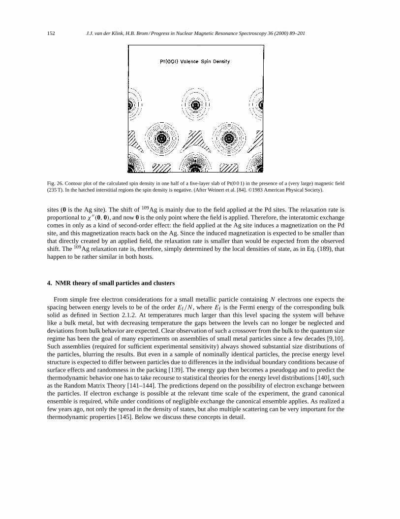
152 J.J. van der Klink, H.B. Brom / Progress in Nuclear Magnetic Resonance Spectroscopy 36 (2000) 89–201
Fig. 26. Contour plot of the calculated spin density in one half of a five-layer slab of Pt(0 0 1) in the presence of a (very large) magnetic field(235 T). In the hatched interstitial regions the spin density is negative. (After Weinert et al. [84]. ©1983 American Physical Society).
sites (0 is the Ag site). The shift of109Ag is mainly due to the field applied at the Pd sites. The relaxation rate isproportional toχ ′′(0,0), and now0 is the only point where the field is applied. Therefore, the interatomic exchangecomes in only as a kind of second-order effect: the field applied at the Ag site induces a magnetization on the Pdsite, and this magnetization reacts back on the Ag. Since the induced magnetization is expected to be smaller thanthat directly created by an applied field, the relaxation rate is smaller than would be expected from the observedshift. The109Ag relaxation rate is, therefore, simply determined by the local densities of state, as in Eq. (189), thathappen to be rather similar in both hosts.
4. NMR theory of small particles and clusters
From simple free electron considerations for a small metallic particle containingN electrons one expects thespacing between energy levels to be of the orderEf /N , whereEf is the Fermi energy of the corresponding bulksolid as defined in Section 2.1.2. At temperatures much larger than this level spacing the system will behavelike a bulk metal, but with decreasing temperature the gaps between the levels can no longer be neglected anddeviations from bulk behavior are expected. Clear observation of such a crossover from the bulk to the quantum sizeregime has been the goal of many experiments on assemblies of small metal particles since a few decades [9,10].Such assemblies (required for sufficient experimental sensitivity) always showed substantial size distributions ofthe particles, blurring the results. But even in a sample of nominally identical particles, the precise energy levelstructure is expected to differ between particles due to differences in the individual boundary conditions because ofsurface effects and randomness in the packing [139]. The energy gap then becomes a pseudogap and to predict thethermodynamic behavior one has to take recourse to statistical theories for the energy level distributions [140], suchas the Random Matrix Theory [141–144]. The predictions depend on the possibility of electron exchange betweenthe particles. If electron exchange is possible at the relevant time scale of the experiment, the grand canonicalensemble is required, while under conditions of negligible exchange the canonical ensemble applies. As realized afew years ago, not only the spread in the density of states, but also multiple scattering can be very important for thethermodynamic properties [145]. Below we discuss these concepts in detail.
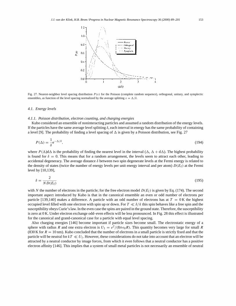
J.J. van der Klink, H.B. Brom / Progress in Nuclear Magnetic Resonance Spectroscopy 36 (2000) 89–201 153
Fig. 27. Nearest-neighbor level spacing distributionP(x) for the Poisson (complete random sequence), orthogonal, unitary, and symplecticensembles, as function of the level spacing normalized by the average splittingx = 1/δ.
4.1. Energy levels
4.1.1. Poisson distribution, electron counting, and charging energiesKubo considered an ensemble of noninteracting particles and assumed a random distribution of the energy levels.
If the particles have the same average level splittingδ, each interval in energy has the same probability of containinga level [9]. The probability of finding a level spacing of1 is given by a Poisson distribution, see Fig. 27
P(1) = 1
δe−1/δ, (194)
whereP(1)d1 is the probability of finding the nearest level in the interval (1,1+ d1). The highest probabilityis found forδ = 0. This means that for a random arrangement, the levels seem to attract each other, leading toaccidental degeneracy. The average distanceδ between two spin degenerate levels at the Fermi energy is related tothe density of states (twice the number of energy levels per unit energy interval and per atom)D(Ef ) at the Fermilevel by [10,139],
δ = 2
ND(Ef )(195)
withN the number of electrons in the particle; for the free electron modelD(Ef ) is given by Eq. (174). The secondimportant aspect introduced by Kubo is that in the canonical ensemble an even or odd number of electrons perparticle [139,140] makes a difference. A particle with an odd number of electrons has atT = 0 K the highestoccupied level filled with one electron with spin up or down. ForT � δ/k this spin behaves like a free spin and thesusceptibility obeys Curie’s law. In the even case the spins are paired in the ground state. Therefore, the susceptibilityis zero at 0 K. Under electron exchange odd–even effects will be less pronounced. In Fig. 28 this effect is illustratedfor the canonical and grand-canonical case for a particle with equal level spacing.
Also charging energies [146] become important if particle sizes become small. The electrostatic energy of asphere with radiusR and one extra electron isU1 = e2/(8πε0R). This quantity becomes very large for smallR(830 K forR = 10 nm). Kubo concluded that the number of electrons in a small particle is strictly fixed and that theparticle will be neutral forkT � U1. However, these considerations do not take into account that an electron will beattracted by a neutral conductor by image forces, from which it even follows that a neutral conductor has a positiveelectron affinity [146]. This implies that a system of small metal particles is not necessarily an ensemble of neutral
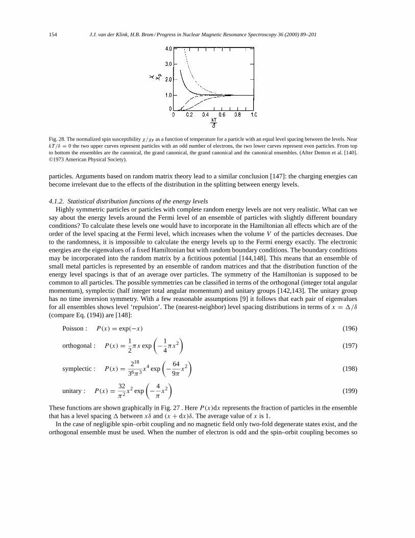
154 J.J. van der Klink, H.B. Brom / Progress in Nuclear Magnetic Resonance Spectroscopy 36 (2000) 89–201
Fig. 28. The normalized spin susceptibilityχ/χP as a function of temperature for a particle with an equal level spacing between the levels. NearkT /δ = 0 the two upper curves represent particles with an odd number of electrons, the two lower curves represent even particles. From topto bottom the ensembles are the canonical, the grand canonical, the grand canonical and the canonical ensembles. (After Denton et al. [140].©1973 American Physical Society).
particles. Arguments based on random matrix theory lead to a similar conclusion [147]: the charging energies canbecome irrelevant due to the effects of the distribution in the splitting between energy levels.
4.1.2. Statistical distribution functions of the energy levelsHighly symmetric particles or particles with complete random energy levels are not very realistic. What can we
say about the energy levels around the Fermi level of an ensemble of particles with slightly different boundaryconditions? To calculate these levels one would have to incorporate in the Hamiltonian all effects which are of theorder of the level spacing at the Fermi level, which increases when the volumeV of the particles decreases. Dueto the randomness, it is impossible to calculate the energy levels up to the Fermi energy exactly. The electronicenergies are the eigenvalues of a fixed Hamiltonian but with random boundary conditions. The boundary conditionsmay be incorporated into the random matrix by a fictitious potential [144,148]. This means that an ensemble ofsmall metal particles is represented by an ensemble of random matrices and that the distribution function of theenergy level spacings is that of an average over particles. The symmetry of the Hamiltonian is supposed to becommon to all particles. The possible symmetries can be classified in terms of the orthogonal (integer total angularmomentum), symplectic (half integer total angular momentum) and unitary groups [142,143]. The unitary grouphas no time inversion symmetry. With a few reasonable assumptions [9] it follows that each pair of eigenvaluesfor all ensembles shows level ‘repulsion’. The (nearest-neighbor) level spacing distributions in terms ofx = 1/δ(compare Eq. (194)) are [148]:
Poisson : P(x) = exp(−x) (196)
orthogonal : P(x) = 1
2πx exp
(−1
4πx2
)(197)
symplectic : P(x) = 218
36π3x4 exp
(− 64
9πx2)
(198)
unitary : P(x) = 32
π2x2 exp
(− 4
πx2)
(199)
These functions are shown graphically in Fig. 27 . HereP(x)dx represents the fraction of particles in the ensemblethat has a level spacing1 betweenxδ and(x + dx)δ. The average value ofx is 1.
In the case of negligible spin–orbit coupling and no magnetic field only two-fold degenerate states exist, and theorthogonal ensemble must be used. When the number of electron is odd and the spin–orbit coupling becomes so
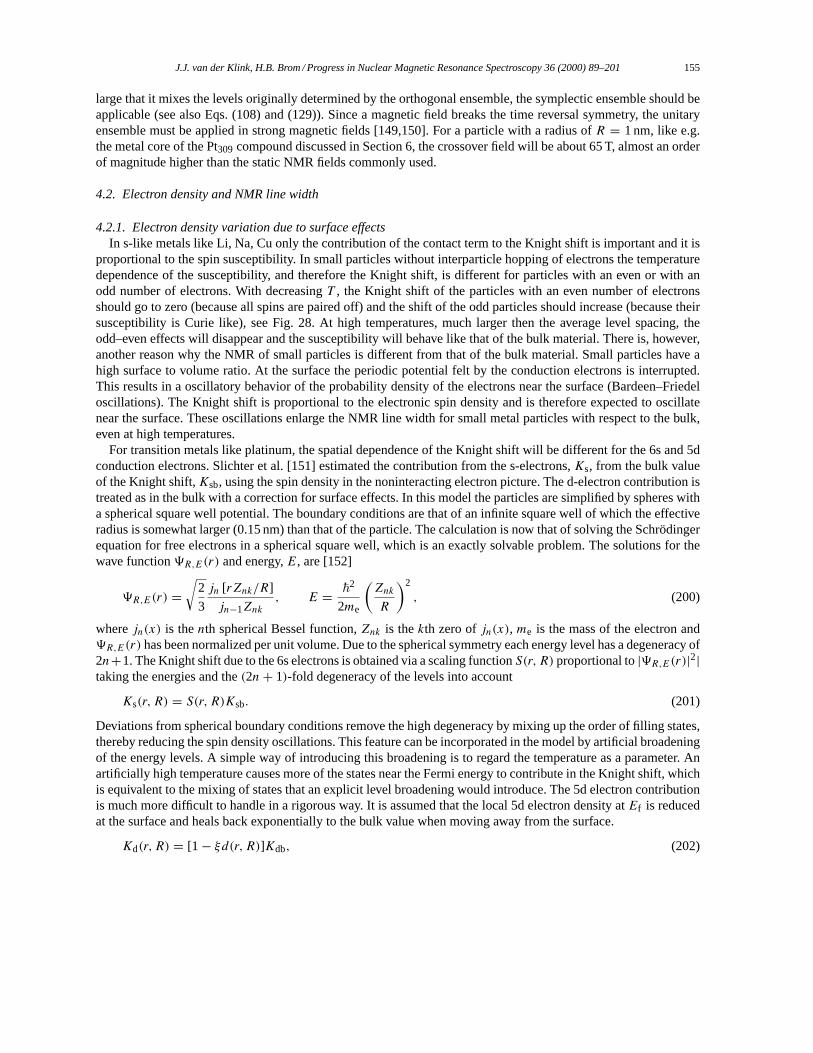
J.J. van der Klink, H.B. Brom / Progress in Nuclear Magnetic Resonance Spectroscopy 36 (2000) 89–201 155
large that it mixes the levels originally determined by the orthogonal ensemble, the symplectic ensemble should beapplicable (see also Eqs. (108) and (129)). Since a magnetic field breaks the time reversal symmetry, the unitaryensemble must be applied in strong magnetic fields [149,150]. For a particle with a radius ofR = 1 nm, like e.g.the metal core of the Pt309 compound discussed in Section 6, the crossover field will be about 65 T, almost an orderof magnitude higher than the static NMR fields commonly used.
4.2. Electron density and NMR line width
4.2.1. Electron density variation due to surface effectsIn s-like metals like Li, Na, Cu only the contribution of the contact term to the Knight shift is important and it is
proportional to the spin susceptibility. In small particles without interparticle hopping of electrons the temperaturedependence of the susceptibility, and therefore the Knight shift, is different for particles with an even or with anodd number of electrons. With decreasingT , the Knight shift of the particles with an even number of electronsshould go to zero (because all spins are paired off) and the shift of the odd particles should increase (because theirsusceptibility is Curie like), see Fig. 28. At high temperatures, much larger then the average level spacing, theodd–even effects will disappear and the susceptibility will behave like that of the bulk material. There is, however,another reason why the NMR of small particles is different from that of the bulk material. Small particles have ahigh surface to volume ratio. At the surface the periodic potential felt by the conduction electrons is interrupted.This results in a oscillatory behavior of the probability density of the electrons near the surface (Bardeen–Friedeloscillations). The Knight shift is proportional to the electronic spin density and is therefore expected to oscillatenear the surface. These oscillations enlarge the NMR line width for small metal particles with respect to the bulk,even at high temperatures.
For transition metals like platinum, the spatial dependence of the Knight shift will be different for the 6s and 5dconduction electrons. Slichter et al. [151] estimated the contribution from the s-electrons,Ks, from the bulk valueof the Knight shift,Ksb, using the spin density in the noninteracting electron picture. The d-electron contribution istreated as in the bulk with a correction for surface effects. In this model the particles are simplified by spheres witha spherical square well potential. The boundary conditions are that of an infinite square well of which the effectiveradius is somewhat larger (0.15 nm) than that of the particle. The calculation is now that of solving the Schrödingerequation for free electrons in a spherical square well, which is an exactly solvable problem. The solutions for thewave function9R,E(r) and energy,E, are [152]
9R,E(r) =√
2
3
jn [rZnk/R]
jn−1Znk, E = ~
2
2me
(Znk
R
)2
, (200)
wherejn(x) is thenth spherical Bessel function,Znk is thekth zero ofjn(x), me is the mass of the electron and9R,E(r) has been normalized per unit volume. Due to the spherical symmetry each energy level has a degeneracy of2n+1. The Knight shift due to the 6s electrons is obtained via a scaling functionS(r, R) proportional to|9R,E(r)|2|taking the energies and the(2n+ 1)-fold degeneracy of the levels into account
Ks(r, R) = S(r, R)Ksb. (201)
Deviations from spherical boundary conditions remove the high degeneracy by mixing up the order of filling states,thereby reducing the spin density oscillations. This feature can be incorporated in the model by artificial broadeningof the energy levels. A simple way of introducing this broadening is to regard the temperature as a parameter. Anartificially high temperature causes more of the states near the Fermi energy to contribute in the Knight shift, whichis equivalent to the mixing of states that an explicit level broadening would introduce. The 5d electron contributionis much more difficult to handle in a rigorous way. It is assumed that the local 5d electron density atEf is reducedat the surface and heals back exponentially to the bulk value when moving away from the surface.
Kd(r, R) = [1− ξd(r, R)]Kdb, (202)
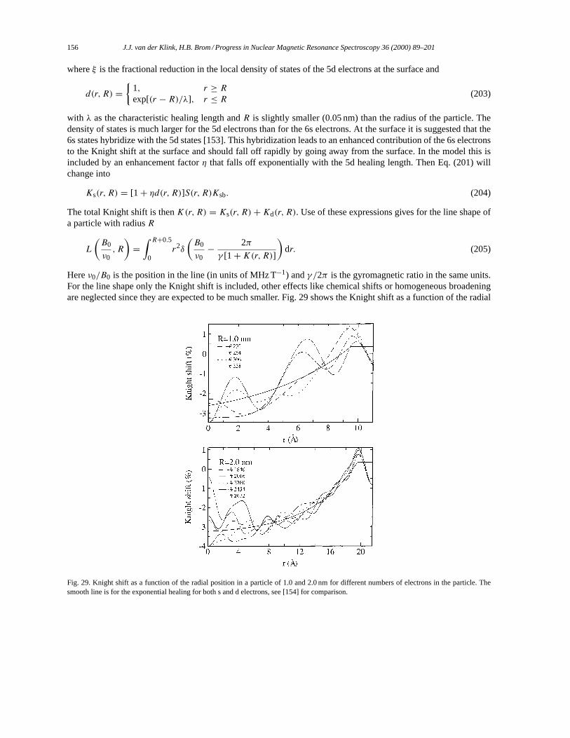
156 J.J. van der Klink, H.B. Brom / Progress in Nuclear Magnetic Resonance Spectroscopy 36 (2000) 89–201
whereξ is the fractional reduction in the local density of states of the 5d electrons at the surface and
d(r, R) ={
1, r ≥ Rexp[(r − R)/λ], r ≤ R (203)
with λ as the characteristic healing length andR is slightly smaller (0.05 nm) than the radius of the particle. Thedensity of states is much larger for the 5d electrons than for the 6s electrons. At the surface it is suggested that the6s states hybridize with the 5d states [153]. This hybridization leads to an enhanced contribution of the 6s electronsto the Knight shift at the surface and should fall off rapidly by going away from the surface. In the model this isincluded by an enhancement factorη that falls off exponentially with the 5d healing length. Then Eq. (201) willchange into
Ks(r, R) = [1+ ηd(r, R)]S(r, R)Ksb. (204)
The total Knight shift is thenK(r, R) = Ks(r, R)+Kd(r, R). Use of these expressions gives for the line shape ofa particle with radiusR
L
(B0
ν0, R
)=∫ R+0.5
0r2δ
(B0
ν0− 2π
γ [1+K(r, R)])
dr. (205)
Hereν0/B0 is the position in the line (in units of MHz T−1) andγ /2π is the gyromagnetic ratio in the same units.For the line shape only the Knight shift is included, other effects like chemical shifts or homogeneous broadeningare neglected since they are expected to be much smaller. Fig. 29 shows the Knight shift as a function of the radial
Fig. 29. Knight shift as a function of the radial position in a particle of 1.0 and 2.0 nm for different numbers of electrons in the particle. Thesmooth line is for the exponential healing for both s and d electrons, see [154] for comparison.
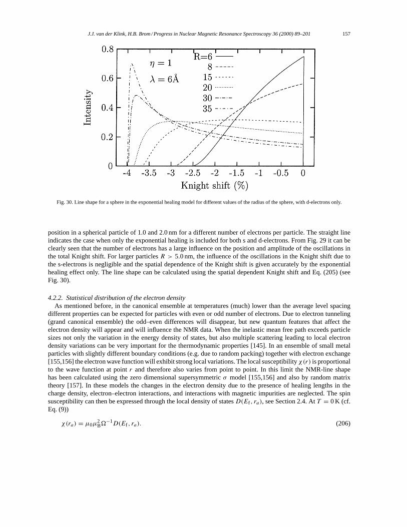
J.J. van der Klink, H.B. Brom / Progress in Nuclear Magnetic Resonance Spectroscopy 36 (2000) 89–201 157
Fig. 30. Line shape for a sphere in the exponential healing model for different values of the radius of the sphere, with d-electrons only.
position in a spherical particle of 1.0 and 2.0 nm for a different number of electrons per particle. The straight lineindicates the case when only the exponential healing is included for both s and d-electrons. From Fig. 29 it can beclearly seen that the number of electrons has a large influence on the position and amplitude of the oscillations inthe total Knight shift. For larger particlesR > 5.0 nm, the influence of the oscillations in the Knight shift due tothe s-electrons is negligible and the spatial dependence of the Knight shift is given accurately by the exponentialhealing effect only. The line shape can be calculated using the spatial dependent Knight shift and Eq. (205) (seeFig. 30).
4.2.2. Statistical distribution of the electron densityAs mentioned before, in the canonical ensemble at temperatures (much) lower than the average level spacing
different properties can be expected for particles with even or odd number of electrons. Due to electron tunneling(grand canonical ensemble) the odd–even differences will disappear, but new quantum features that affect theelectron density will appear and will influence the NMR data. When the inelastic mean free path exceeds particlesizes not only the variation in the energy density of states, but also multiple scattering leading to local electrondensity variations can be very important for the thermodynamic properties [145]. In an ensemble of small metalparticles with slightly different boundary conditions (e.g. due to random packing) together with electron exchange[155,156] the electron wave function will exhibit strong local variations. The local susceptibilityχ(r) is proportionalto the wave function at pointr and therefore also varies from point to point. In this limit the NMR-line shapehas been calculated using the zero dimensional supersymmetricσ model [155,156] and also by random matrixtheory [157]. In these models the changes in the electron density due to the presence of healing lengths in thecharge density, electron–electron interactions, and interactions with magnetic impurities are neglected. The spinsusceptibility can then be expressed through the local density of statesD(Ef , ra), see Section 2.4. AtT = 0 K (cf.Eq. (9))
χ(ra) = µ0µ2B�−1D(Ef , ra). (206)
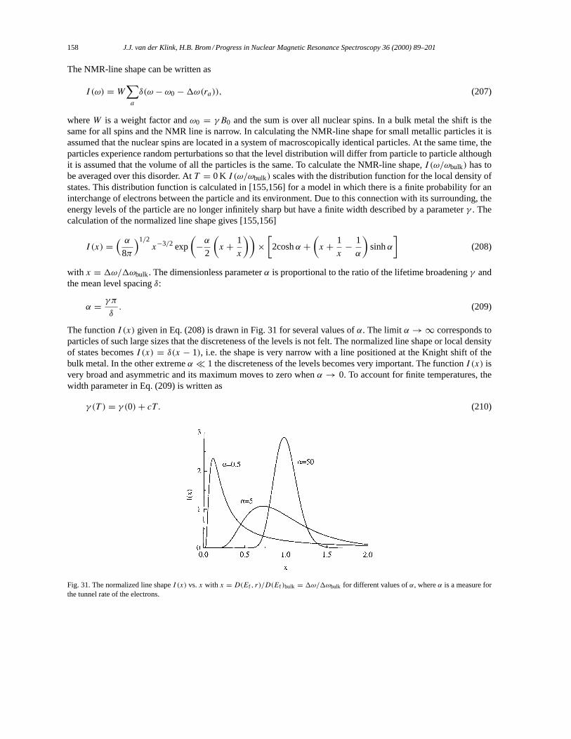
158 J.J. van der Klink, H.B. Brom / Progress in Nuclear Magnetic Resonance Spectroscopy 36 (2000) 89–201
The NMR-line shape can be written as
I (ω) = W∑a
δ(ω − ω0 −1ω(ra)), (207)
whereW is a weight factor andω0 = γB0 and the sum is over all nuclear spins. In a bulk metal the shift is thesame for all spins and the NMR line is narrow. In calculating the NMR-line shape for small metallic particles it isassumed that the nuclear spins are located in a system of macroscopically identical particles. At the same time, theparticles experience random perturbations so that the level distribution will differ from particle to particle althoughit is assumed that the volume of all the particles is the same. To calculate the NMR-line shape,I (ω/ωbulk) has tobe averaged over this disorder. AtT = 0 K I (ω/ωbulk) scales with the distribution function for the local density ofstates. This distribution function is calculated in [155,156] for a model in which there is a finite probability for aninterchange of electrons between the particle and its environment. Due to this connection with its surrounding, theenergy levels of the particle are no longer infinitely sharp but have a finite width described by a parameterγ . Thecalculation of the normalized line shape gives [155,156]
I (x) =( α
8π
)1/2x−3/2 exp
(−α
2
(x + 1
x
))×[2coshα +
(x + 1
x− 1
α
)sinhα
](208)
with x = 1ω/1ωbulk. The dimensionless parameterα is proportional to the ratio of the lifetime broadeningγ andthe mean level spacingδ:
α = γπ
δ. (209)
The functionI (x) given in Eq. (208) is drawn in Fig. 31 for several values ofα. The limitα→∞ corresponds toparticles of such large sizes that the discreteness of the levels is not felt. The normalized line shape or local densityof states becomesI (x) = δ(x − 1), i.e. the shape is very narrow with a line positioned at the Knight shift of thebulk metal. In the other extremeα � 1 the discreteness of the levels becomes very important. The functionI (x) isvery broad and asymmetric and its maximum moves to zero whenα → 0. To account for finite temperatures, thewidth parameter in Eq. (209) is written as
γ (T ) = γ (0)+ cT . (210)
Fig. 31. The normalized line shapeI (x) vs.x with x = D(Ef , r)/D(Ef )bulk = 1ω/1ωbulk for different values ofα, whereα is a measure forthe tunnel rate of the electrons.
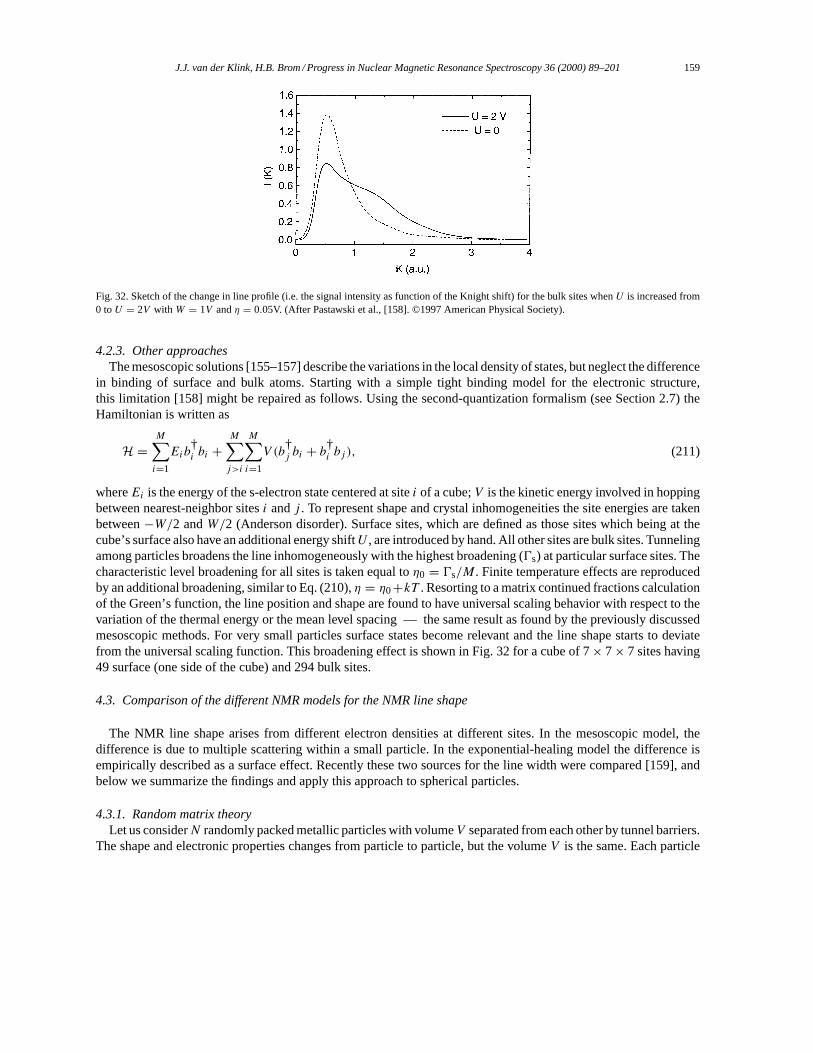
J.J. van der Klink, H.B. Brom / Progress in Nuclear Magnetic Resonance Spectroscopy 36 (2000) 89–201 159
Fig. 32. Sketch of the change in line profile (i.e. the signal intensity as function of the Knight shift) for the bulk sites whenU is increased from0 toU = 2V with W = 1V andη = 0.05V. (After Pastawski et al., [158]. ©1997 American Physical Society).
4.2.3. Other approachesThe mesoscopic solutions [155–157] describe the variations in the local density of states, but neglect the difference
in binding of surface and bulk atoms. Starting with a simple tight binding model for the electronic structure,this limitation [158] might be repaired as follows. Using the second-quantization formalism (see Section 2.7) theHamiltonian is written as
H =M∑i=1
Eib†i bi +
M∑j>i
M∑i=1
V (b†j bi + b†i bj ), (211)
whereEi is the energy of the s-electron state centered at sitei of a cube;V is the kinetic energy involved in hoppingbetween nearest-neighbor sitesi andj . To represent shape and crystal inhomogeneities the site energies are takenbetween−W/2 andW/2 (Anderson disorder). Surface sites, which are defined as those sites which being at thecube’s surface also have an additional energy shiftU , are introduced by hand. All other sites are bulk sites. Tunnelingamong particles broadens the line inhomogeneously with the highest broadening (0s) at particular surface sites. Thecharacteristic level broadening for all sites is taken equal toη0 = 0s/M. Finite temperature effects are reproducedby an additional broadening, similar to Eq. (210),η = η0+kT . Resorting to a matrix continued fractions calculationof the Green’s function, the line position and shape are found to have universal scaling behavior with respect to thevariation of the thermal energy or the mean level spacing — the same result as found by the previously discussedmesoscopic methods. For very small particles surface states become relevant and the line shape starts to deviatefrom the universal scaling function. This broadening effect is shown in Fig. 32 for a cube of 7× 7× 7 sites having49 surface (one side of the cube) and 294 bulk sites.
4.3. Comparison of the different NMR models for the NMR line shape
The NMR line shape arises from different electron densities at different sites. In the mesoscopic model, thedifference is due to multiple scattering within a small particle. In the exponential-healing model the difference isempirically described as a surface effect. Recently these two sources for the line width were compared [159], andbelow we summarize the findings and apply this approach to spherical particles.
4.3.1. Random matrix theoryLet us considerN randomly packed metallic particles with volumeV separated from each other by tunnel barriers.
The shape and electronic properties changes from particle to particle, but the volumeV is the same. Each particle

160 J.J. van der Klink, H.B. Brom / Progress in Nuclear Magnetic Resonance Spectroscopy 36 (2000) 89–201
contains on the averageM electrons. The system is, therefore, an(N × M) electron system. The energy leveldistribution is quasi continuous, but each corresponding eigenfunction is supposed to be well localized in one of theN particles. Therefore, this model is referred to as the tunnelling/localization model. The particles are numberedby n and the energy levels within a particle byk. It is assumed that the probability distribution of the energy of anelectron in a level (n,k) is given by a LorentzianL(E − Enk ) with width γ /2 independent ofn andk.
L(E) = γ
2π
[E2+
(γ2
)2]−1
. (212)
The charge distribution|ψnk (r)|2 is not supposed to be uniform. To calculate the thermodynamic properties thereare two steps involved [139]. The first step is to average over an ensemble of particles which are all completelyidentical to particlen. The total number of electrons is supposed to be so large and the temperature so low that thechemical potentialζ (see Section 2.1.2) is temperature independent. Due to electron tunneling or hoppingζ is equalin all the particles. The second step takes into account the differences in energy levels for different particles. Thethermodynamic average for the susceptibility of particlen, χn, is given by
χn = −2µ0µ2B
V
∑k
∫L(Enk − E)
∂f
∂EdE (213)
and the second step is the average over particlesn
χ = N−1∑n
χn. (214)
The second moment of the susceptibility is defined by
1χ2 = N−1∑n
(χn − χ)2. (215)
Using the same methods the average Knight shift (or center of gravity of the line) becomes
K = 23χ. (216)
The expression for the second moment of the resonance lines not only depends on1χ2, but also on the two levelcorrelation function and the variations in|ψnk (r)|2 within the particles. From random matrix theory explicit formsof the level correlation functions can be obtained. The second moment of the Knight shift becomes
1K2 = 491χ
2+ 49(πα)
−1χ2A = K2(πα)−1(g(α)+ A). (217)
Theα in Eq. (217) is a levelwidth parameter similar to Eq. (209), andA has the value of 2/β with β = 1,2,4 forthe orthogonal, unitary and symplectic ensembles [157]. The first term of Eq. (217) comes from the variation insusceptibility due to the difference in energy levels aroundEf between particles: the stronger the level repulsion theless variation inχ , see Fig. 33. The second term comes from the variation of the wave functions within the particles.At high temperatures, this means large values ofα, the first contribution vanishes, and the variation of the wavefunction dominates. At low temperatures, i.e. small values ofα, the influences of both terms are of equal size.
4.3.2. Exponential healingThe exponential healing model focuses on surface effects. For comparison with the multiple scattering model let
us consider an infinite slab of thickness 2d. The Knight shift varies with distancex from the center of the slab as
K(x)
Kb= 1− η exp
(x − dλ
)(218)
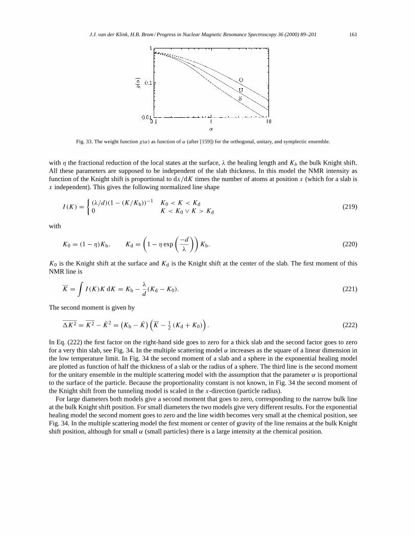
J.J. van der Klink, H.B. Brom / Progress in Nuclear Magnetic Resonance Spectroscopy 36 (2000) 89–201 161
Fig. 33. The weight functiong(α) as function ofα (after [159]) for the orthogonal, unitary, and symplectic ensemble.
with η the fractional reduction of the local states at the surface,λ the healing length andKb the bulk Knight shift.All these parameters are supposed to be independent of the slab thickness. In this model the NMR intensity asfunction of the Knight shift is proportional to dx/dK times the number of atoms at positionx (which for a slab isx independent). This gives the following normalized line shape
I (K) ={(λ/d)(1− (K/Kb))
−1 K0 < K < Kd0 K < K0 ∨K > Kd
(219)
with
K0 = (1− η)Kb, Kd =(
1− η exp
(−dλ
))Kb. (220)
K0 is the Knight shift at the surface andKd is the Knight shift at the center of the slab. The first moment of thisNMR line is
K =∫I (K)K dK = Kb− λ
d(Kd −K0). (221)
The second moment is given by
1K2 = K2− K2 = (Kb− K) (K − 1
2 (Kd +K0)). (222)
In Eq. (222) the first factor on the right-hand side goes to zero for a thick slab and the second factor goes to zerofor a very thin slab, see Fig. 34. In the multiple scattering modelα increases as the square of a linear dimension inthe low temperature limit. In Fig. 34 the second moment of a slab and a sphere in the exponential healing modelare plotted as function of half the thickness of a slab or the radius of a sphere. The third line is the second momentfor the unitary ensemble in the multiple scattering model with the assumption that the parameterα is proportionalto the surface of the particle. Because the proportionality constant is not known, in Fig. 34 the second moment ofthe Knight shift from the tunneling model is scaled in thex-direction (particle radius).
For large diameters both models give a second moment that goes to zero, corresponding to the narrow bulk lineat the bulk Knight shift position. For small diameters the two models give very different results. For the exponentialhealing model the second moment goes to zero and the line width becomes very small at the chemical position, seeFig. 34. In the multiple scattering model the first moment or center of gravity of the line remains at the bulk Knightshift position, although for smallα (small particles) there is a large intensity at the chemical position.
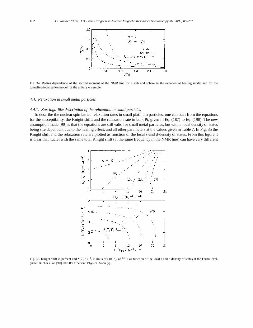
162 J.J. van der Klink, H.B. Brom / Progress in Nuclear Magnetic Resonance Spectroscopy 36 (2000) 89–201
Fig. 34. Radius dependence of the second moment of the NMR line for a slab and sphere in the exponential healing model and for thetunneling/localization model for the unitary ensemble.
4.4. Relaxation in small metal particles
4.4.1. Korringa-like description of the relaxation in small particlesTo describe the nuclear spin lattice relaxation rates in small platinum particles, one can start from the equations
for the susceptibility, the Knight shift, and the relaxation rate in bulk Pt, given in Eq. (187) to Eq. (190). The newassumption made [90] is that the equations are still valid for small metal particles, but with a local density of statesbeing site dependent due to the healing effect, and all other parameters at the values given in Table 7. In Fig. 35 theKnight shift and the relaxation rate are plotted as function of the local s-and d-density of states. From this figure itis clear that nuclei with the same total Knight shift (at the same frequency in the NMR line) can have very different
Fig. 35. Knight shift in percent andS(T1T )−1, in units of (10−6), of 195Pt as function of the local s and d density of states at the Fermi level.
(After Bucher et al. [90]. ©1988 American Physical Society).
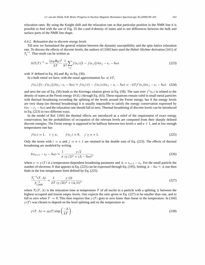
J.J. van der Klink, H.B. Brom / Progress in Nuclear Magnetic Resonance Spectroscopy 36 (2000) 89–201 163
relaxation rates. By using the Knight shift and the relaxation rate at that particular position in the NMR line it ispossible to find with the use of Fig. 35 the s-and d-density of states and to see differences between the bulk andsurface parts of the NMR line shape.
4.4.2. Relaxation due to discrete energy levelsTill now we formulated the general relation between the dynamic susceptibility and the spin–lattice relaxation
rate. To discuss the effects of discrete levels, the authors of [160] have used the Hebel–Slichter derivation [161] ofT −1
1 . That result can be written as
S(T1T )−1 = (µBBhf)
2
kT
1
N2
∑i,j
f (εi)(1− f (εj )
)δ(εj − εi − ~ω) (223)
with N defined in Eq. (6) andBhf in Eq. (36).In a bulk metal we have, with the usual approximation~ω � kT ,
f (εi)(1−f (εj )
)δ(εj−εi − ~ω) ≈ f (εi) (1− f (εi)) δ(εj − εi − ~ω) = −kTf ′(εi)δ(εj − εi − ~ω) (224)
and next the use of Eq. (56) leads to the Korringa relation given in Eq. (58). The sum overf ′(εi) is related to thedensity of states at the Fermi energyD(Ef ) through Eq. (63). These equations remain valid in small metal particleswith thermal broadening exceeding the splitting of the levels around the Fermi energy, but if the energy levelsare very sharp (no thermal broadening) it is usually impossible to satisfy the energy conservation expressed byδ(εi − εj − ~ω) and the relaxation rate should fall to zero. Thermal broadening of discrete levels can be introducedin Eq. (223) in two different ways.
In the model of Ref. [160] the thermal effects are introduced as a relief of the requirement of exact energyconservation; but the probabilities of occupation of the relevant levels are computed from their sharply defineddiscrete energies. The Fermi energy is supposed to be halfway between two levelsn andn+ 1, and at low enoughtemperatures one has
f (εi) = 1, i ≤ n, f (εj ) = 0, j ≥ n+ 1. (225)
Only the terms withi = n andj = n + 1 are retained in the double sum of Eq. (223). The effects of thermalbroadening are modeled by writing
δ(εn+1− εn − ~ω) ≈ 1
π
γ/2
(γ /2)2+ (1− ~ω)2 , (226)
whereγ = γ (T ) is a temperature-dependent broadening parameter and1 = εn+1− εn. For the small particle thenumber of electronsN that appears in Eq. (223) can be expressed through Eq. (195). Setting1− ~ω ≈ 1 one thenfinds in the low-temperature limit defined by Eq. (225)
T −11 (T ,1)
T −11,bulk
= δ
kT
γ /2δ
(γ /2δ)2+ (1/δ)2 , (227)
whereT1(T ,1) is the relaxation time at temperatureT of all nuclei in a particle with a splitting1 between thehighest occupied and lowest empty levels. One expects the ratio given in Eq. (227) to be smaller than one, and tofall to zero whenT → 0. This then requires thatγ (T ) goes to zero faster than linear in the temperature. In [160]γ (T ) was chosen to depend on the level splitting and on the temperature as
γ (T ,1) = γ0(T )exp
(−1kT
). (228)
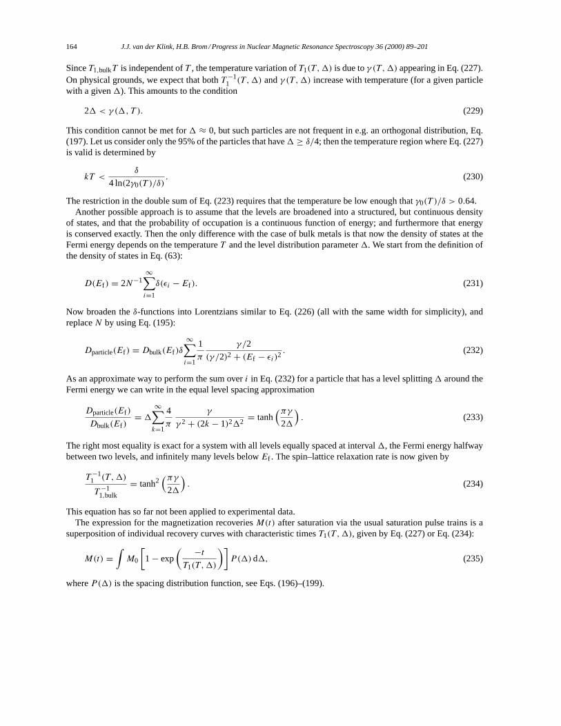
164 J.J. van der Klink, H.B. Brom / Progress in Nuclear Magnetic Resonance Spectroscopy 36 (2000) 89–201
SinceT1,bulkT is independent ofT , the temperature variation ofT1(T ,1) is due toγ (T ,1) appearing in Eq. (227).On physical grounds, we expect that bothT −1
1 (T ,1) andγ (T ,1) increase with temperature (for a given particlewith a given1). This amounts to the condition
21 < γ (1, T ). (229)
This condition cannot be met for1 ≈ 0, but such particles are not frequent in e.g. an orthogonal distribution, Eq.(197). Let us consider only the 95% of the particles that have1 ≥ δ/4; then the temperature region where Eq. (227)is valid is determined by
kT <δ
4 ln(2γ0(T )/δ). (230)
The restriction in the double sum of Eq. (223) requires that the temperature be low enough thatγ0(T )/δ > 0.64.Another possible approach is to assume that the levels are broadened into a structured, but continuous density
of states, and that the probability of occupation is a continuous function of energy; and furthermore that energyis conserved exactly. Then the only difference with the case of bulk metals is that now the density of states at theFermi energy depends on the temperatureT and the level distribution parameter1. We start from the definition ofthe density of states in Eq. (63):
D(Ef ) = 2N−1∞∑i=1
δ(εi − Ef ). (231)
Now broaden theδ-functions into Lorentzians similar to Eq. (226) (all with the same width for simplicity), andreplaceN by using Eq. (195):
Dparticle(Ef ) = Dbulk(Ef )δ
∞∑i=1
1
π
γ/2
(γ /2)2+ (Ef − εi)2 . (232)
As an approximate way to perform the sum overi in Eq. (232) for a particle that has a level splitting1 around theFermi energy we can write in the equal level spacing approximation
Dparticle(Ef )
Dbulk(Ef )= 1
∞∑k=1
4
π
γ
γ 2+ (2k − 1)212= tanh
(πγ21
). (233)
The right most equality is exact for a system with all levels equally spaced at interval1, the Fermi energy halfwaybetween two levels, and infinitely many levels belowEf . The spin–lattice relaxation rate is now given by
T −11 (T ,1)
T −11,bulk
= tanh2(πγ
21
). (234)
This equation has so far not been applied to experimental data.The expression for the magnetization recoveriesM(t) after saturation via the usual saturation pulse trains is a
superposition of individual recovery curves with characteristic timesT1(T ,1), given by Eq. (227) or Eq. (234):
M(t) =∫M0
[1− exp
( −tT1(T ,1)
)]P(1)d1, (235)
whereP(1) is the spacing distribution function, see Eqs. (196)–(199).
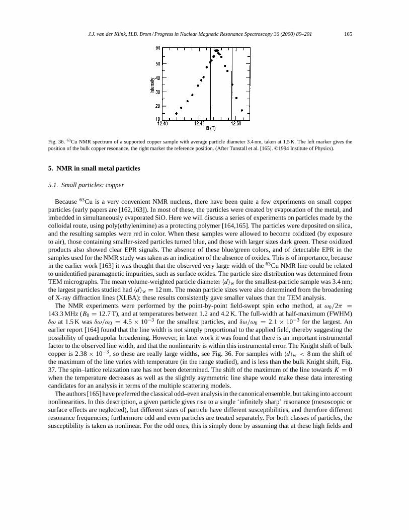
J.J. van der Klink, H.B. Brom / Progress in Nuclear Magnetic Resonance Spectroscopy 36 (2000) 89–201 165
Fig. 36.63Cu NMR spectrum of a supported copper sample with average particle diameter 3.4 nm, taken at 1.5 K. The left marker gives theposition of the bulk copper resonance, the right marker the reference position. (After Tunstall et al. [165]. ©1994 Institute of Physics).
5. NMR in small metal particles
5.1. Small particles: copper
Because63Cu is a very convenient NMR nucleus, there have been quite a few experiments on small copperparticles (early papers are [162,163]). In most of these, the particles were created by evaporation of the metal, andimbedded in simultaneously evaporated SiO. Here we will discuss a series of experiments on particles made by thecolloidal route, using poly(ethylenimine) as a protecting polymer [164,165]. The particles were deposited on silica,and the resulting samples were red in color. When these samples were allowed to become oxidized (by exposureto air), those containing smaller-sized particles turned blue, and those with larger sizes dark green. These oxidizedproducts also showed clear EPR signals. The absence of these blue/green colors, and of detectable EPR in thesamples used for the NMR study was taken as an indication of the absence of oxides. This is of importance, becausein the earlier work [163] it was thought that the observed very large width of the63Cu NMR line could be relatedto unidentified paramagnetic impurities, such as surface oxides. The particle size distribution was determined fromTEM micrographs. The mean volume-weighted particle diameter〈d〉w for the smallest-particle sample was 3.4 nm;the largest particles studied had〈d〉w = 12 nm. The mean particle sizes were also determined from the broadeningof X-ray diffraction lines (XLBA): these results consistently gave smaller values than the TEM analysis.
The NMR experiments were performed by the point-by-point field-swept spin echo method, atω0/2π =143.3 MHz (B0 = 12.7 T), and at temperatures between 1.2 and 4.2 K. The full-width at half-maximum (FWHM)δω at 1.5 K wasδω/ω0 = 4.5× 10⁻³ for the smallest particles, andδω/ω0 = 2.1× 10⁻³ for the largest. Anearlier report [164] found that the line width is not simply proportional to the applied field, thereby suggesting thepossibility of quadrupolar broadening. However, in later work it was found that there is an important instrumentalfactor to the observed line width, and that the nonlinearity is within this instrumental error. The Knight shift of bulkcopper is 2.38× 10⁻³, so these are really large widths, see Fig. 36. For samples with〈d〉w < 8 nm the shift ofthe maximum of the line varies with temperature (in the range studied), and is less than the bulk Knight shift, Fig.37. The spin–lattice relaxation rate has not been determined. The shift of the maximum of the line towardsK = 0when the temperature decreases as well as the slightly asymmetric line shape would make these data interestingcandidates for an analysis in terms of the multiple scattering models.
The authors [165] have preferred the classical odd–even analysis in the canonical ensemble, but taking into accountnonlinearities. In this description, a given particle gives rise to a single ‘infinitely sharp’ resonance (mesoscopic orsurface effects are neglected), but different sizes of particle have different susceptibilities, and therefore differentresonance frequencies; furthermore odd and even particles are treated separately. For both classes of particles, thesusceptibility is taken as nonlinear. For the odd ones, this is simply done by assuming that at these high fields and
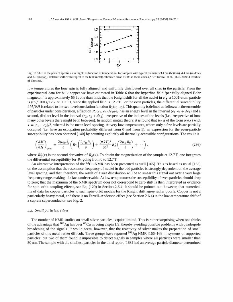
166 J.J. van der Klink, H.B. Brom / Progress in Nuclear Magnetic Resonance Spectroscopy 36 (2000) 89–201
Fig. 37. Shift at the peak of spectra as in Fig 36 as function of temperature, for samples with typical diameters 3.4 nm (bottom), 4.4 nm (middle)and 8.0 nm (top). Relative shift, with respect to the bulk metal; estimated error±0.05 in these units. (After Tunstall et al. [165]. ©1994 Instituteof Physics).
low temperatures the lone spin is fully aligned, and uniformly distributed over all sites in the particle. From theexperimental data for bulk copper we have estimated in Table 6 that the hyperfine field ‘per fully aligned Bohrmagneton’ is approximately 65 T; one than finds that the Knight shift for all the nuclei in e.g. a 1001-atom particleis (65/1001)/12.7 ≈ 0.0051, since the applied field is 12.7 T. For the even particles, the differential susceptibility∂M/∂H is related to the two-level correlation functionR2(ε1, ε2). This quantity is defined as follows: in the ensembleof particles under consideration, a fractionR2(ε1, ε2)dε1dε2 has an energy level in the interval(ε1, ε1+ dε1) and asecond, distinct level in the interval(ε2, ε2+ dε2), irrespective of the indices of the levels (i.e. irrespective of howmany other levels there might be in between). In random matrix theory, it is found thatR2 is of the formR2(x)withx = |ε1− ε2|/δ, whereδ is the mean level spacing. At very low temperatures, where only a few levels are partiallyoccupied (i.e. have an occupation probability different from 0 and from 1), an expression for the even-particlesusceptibility has been obtained [140] by counting explicitly all thermally accessible configurations. The result is(
∂M
∂H
)even= 2µ0µ
2B
δ
(R2
(2µBB0
δ
)+ (πkT )
2
6δ2R′′2
(2µBB0
δ
)+ · · ·
), (236)
whereR′′2(x) is the second derivative ofR2(x). To obtain the magnetization of the sample at 12.7 T, one integratesthe differential susceptibility forB0 going from 0 to 12.7 T.
An alternative interpretation of the63Cu NMR has been presented as well [165]. This is based as usual [163]on the assumption that the resonance frequency of nuclei in the odd particles is strongly dependent on the averagelevel spacing, and that, therefore, the result of a size distribution will be to smear this signal out over a very largefrequency range, making it in fact unobservable. At low temperatures the susceptibility of even particles should dropto zero; that the maximum of the NMR spectrum does not correspond to zero shift is then interpreted as evidencefor spin–orbit coupling effects, see Eq. (129) in Section 2.6.4. It should be pointed out, however, that numericalfits of data for copper particles to such spin–orbit models for the Knight shift agree rather poorly. Copper is not aparticularly heavy metal, and there is no Ferrell–Anderson effect (see Section 2.6.4) in the low-temperature shift ofa cuprate superconductor, see Fig. 2.
5.2. Small particles: silver
The number of NMR studies on small silver particles is quite limited. This is rather surprising when one thinksof the advantage that109Ag has over63Cu in being a spin 1/2, thereby avoiding possible problems with quadrupolebroadening of the signals. It would seem, however, that the reactivity of silver makes the preparation of smallparticles of this metal rather difficult. Three groups have reported109Ag NMR [166–168] in systems of supportedparticles: but two of them found it impossible to detect signals in samples where all particles were smaller than50 nm. The sample with the smallest particles in the third report [168] had an average particle diameter determined
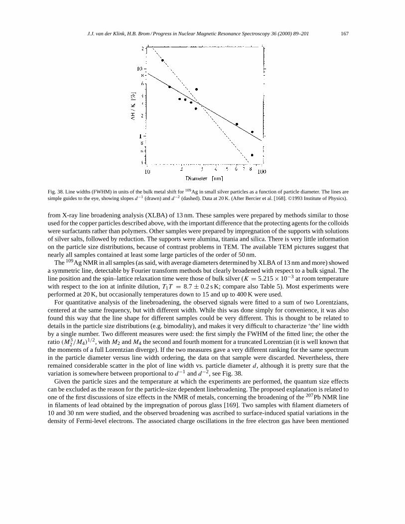
J.J. van der Klink, H.B. Brom / Progress in Nuclear Magnetic Resonance Spectroscopy 36 (2000) 89–201 167
Fig. 38. Line widths (FWHM) in units of the bulk metal shift for109Ag in small silver particles as a function of particle diameter. The lines aresimple guides to the eye, showing slopesd−1 (drawn) andd−2 (dashed). Data at 20 K. (After Bercier et al. [168]. ©1993 Institute of Physics).
from X-ray line broadening analysis (XLBA) of 13 nm. These samples were prepared by methods similar to thoseused for the copper particles described above, with the important difference that the protecting agents for the colloidswere surfactants rather than polymers. Other samples were prepared by impregnation of the supports with solutionsof silver salts, followed by reduction. The supports were alumina, titania and silica. There is very little informationon the particle size distributions, because of contrast problems in TEM. The available TEM pictures suggest thatnearly all samples contained at least some large particles of the order of 50 nm.
The109Ag NMR in all samples (as said, with average diameters determined by XLBA of 13 nm and more) showeda symmetric line, detectable by Fourier transform methods but clearly broadened with respect to a bulk signal. Theline position and the spin–lattice relaxation time were those of bulk silver (K = 5.215× 10⁻³ at room temperaturewith respect to the ion at infinite dilution,T1T = 8.7± 0.2 s K; compare also Table 5). Most experiments wereperformed at 20 K, but occasionally temperatures down to 15 and up to 400 K were used.
For quantitative analysis of the linebroadening, the observed signals were fitted to a sum of two Lorentzians,centered at the same frequency, but with different width. While this was done simply for convenience, it was alsofound this way that the line shape for different samples could be very different. This is thought to be related todetails in the particle size distributions (e.g. bimodality), and makes it very difficult to characterize ‘the’ line widthby a single number. Two different measures were used: the first simply the FWHM of the fitted line; the other theratio(M3
2/M4)1/2, withM2 andM4 the second and fourth moment for a truncated Lorentzian (it is well known that
the moments of a full Lorentzian diverge). If the two measures gave a very different ranking for the same spectrumin the particle diameter versus line width ordering, the data on that sample were discarded. Nevertheless, thereremained considerable scatter in the plot of line width vs. particle diameterd, although it is pretty sure that thevariation is somewhere between proportional tod−1 andd−2, see Fig. 38.
Given the particle sizes and the temperature at which the experiments are performed, the quantum size effectscan be excluded as the reason for the particle-size dependent linebroadening. The proposed explanation is related toone of the first discussions of size effects in the NMR of metals, concerning the broadening of the207Pb NMR linein filaments of lead obtained by the impregnation of porous glass [169]. Two samples with filament diameters of10 and 30 nm were studied, and the observed broadening was ascribed to surface-induced spatial variations in thedensity of Fermi-level electrons. The associated charge oscillations in the free electron gas have been mentioned
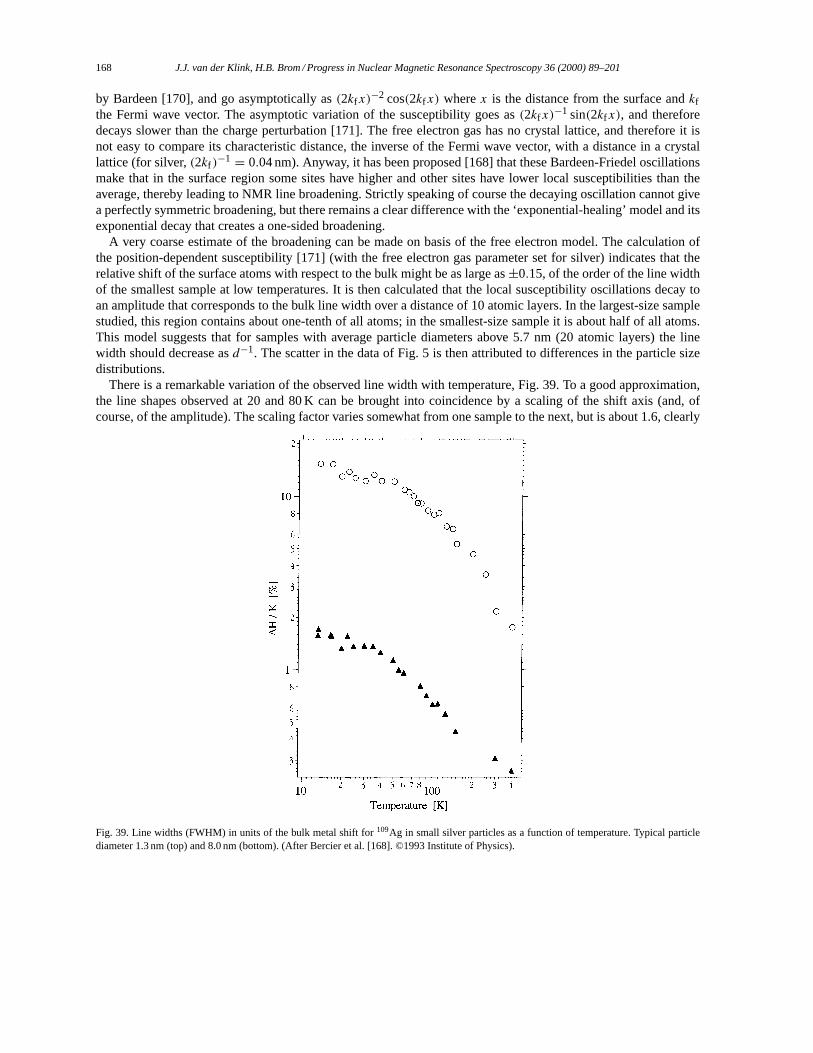
168 J.J. van der Klink, H.B. Brom / Progress in Nuclear Magnetic Resonance Spectroscopy 36 (2000) 89–201
by Bardeen [170], and go asymptotically as(2kf x)−2 cos(2kf x) wherex is the distance from the surface andkf
the Fermi wave vector. The asymptotic variation of the susceptibility goes as(2kf x)−1 sin(2kf x), and therefore
decays slower than the charge perturbation [171]. The free electron gas has no crystal lattice, and therefore it isnot easy to compare its characteristic distance, the inverse of the Fermi wave vector, with a distance in a crystallattice (for silver,(2kf )
−1 = 0.04 nm). Anyway, it has been proposed [168] that these Bardeen-Friedel oscillationsmake that in the surface region some sites have higher and other sites have lower local susceptibilities than theaverage, thereby leading to NMR line broadening. Strictly speaking of course the decaying oscillation cannot givea perfectly symmetric broadening, but there remains a clear difference with the ‘exponential-healing’ model and itsexponential decay that creates a one-sided broadening.
A very coarse estimate of the broadening can be made on basis of the free electron model. The calculation ofthe position-dependent susceptibility [171] (with the free electron gas parameter set for silver) indicates that therelative shift of the surface atoms with respect to the bulk might be as large as±0.15, of the order of the line widthof the smallest sample at low temperatures. It is then calculated that the local susceptibility oscillations decay toan amplitude that corresponds to the bulk line width over a distance of 10 atomic layers. In the largest-size samplestudied, this region contains about one-tenth of all atoms; in the smallest-size sample it is about half of all atoms.This model suggests that for samples with average particle diameters above 5.7 nm (20 atomic layers) the linewidth should decrease asd−1. The scatter in the data of Fig. 5 is then attributed to differences in the particle sizedistributions.
There is a remarkable variation of the observed line width with temperature, Fig. 39. To a good approximation,the line shapes observed at 20 and 80 K can be brought into coincidence by a scaling of the shift axis (and, ofcourse, of the amplitude). The scaling factor varies somewhat from one sample to the next, but is about 1.6, clearly
Fig. 39. Line widths (FWHM) in units of the bulk metal shift for109Ag in small silver particles as a function of temperature. Typical particlediameter 1.3 nm (top) and 8.0 nm (bottom). (After Bercier et al. [168]. ©1993 Institute of Physics).
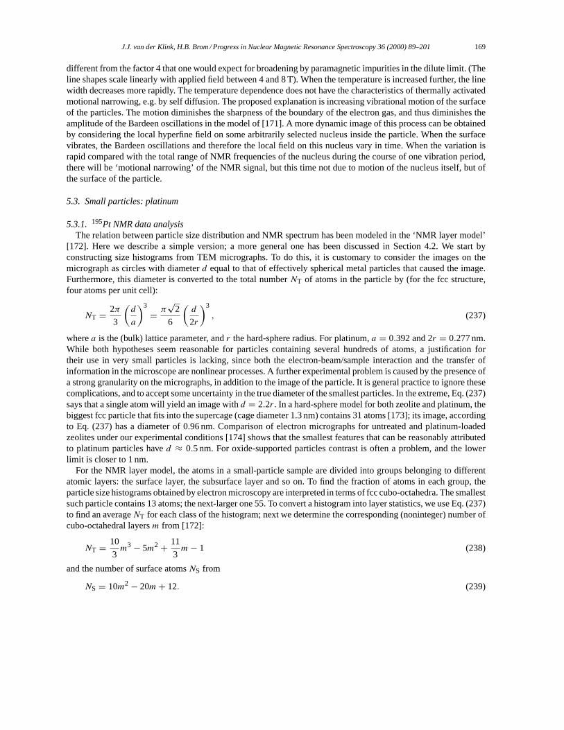
J.J. van der Klink, H.B. Brom / Progress in Nuclear Magnetic Resonance Spectroscopy 36 (2000) 89–201 169
different from the factor 4 that one would expect for broadening by paramagnetic impurities in the dilute limit. (Theline shapes scale linearly with applied field between 4 and 8 T). When the temperature is increased further, the linewidth decreases more rapidly. The temperature dependence does not have the characteristics of thermally activatedmotional narrowing, e.g. by self diffusion. The proposed explanation is increasing vibrational motion of the surfaceof the particles. The motion diminishes the sharpness of the boundary of the electron gas, and thus diminishes theamplitude of the Bardeen oscillations in the model of [171]. A more dynamic image of this process can be obtainedby considering the local hyperfine field on some arbitrarily selected nucleus inside the particle. When the surfacevibrates, the Bardeen oscillations and therefore the local field on this nucleus vary in time. When the variation israpid compared with the total range of NMR frequencies of the nucleus during the course of one vibration period,there will be ‘motional narrowing’ of the NMR signal, but this time not due to motion of the nucleus itself, but ofthe surface of the particle.
5.3. Small particles: platinum
5.3.1. 195Pt NMR data analysisThe relation between particle size distribution and NMR spectrum has been modeled in the ‘NMR layer model’
[172]. Here we describe a simple version; a more general one has been discussed in Section 4.2. We start byconstructing size histograms from TEM micrographs. To do this, it is customary to consider the images on themicrograph as circles with diameterd equal to that of effectively spherical metal particles that caused the image.Furthermore, this diameter is converted to the total numberNT of atoms in the particle by (for the fcc structure,four atoms per unit cell):
NT = 2π
3
(d
a
)3
= π√
2
6
(d
2r
)3
, (237)
wherea is the (bulk) lattice parameter, andr the hard-sphere radius. For platinum,a = 0.392 and 2r = 0.277 nm.While both hypotheses seem reasonable for particles containing several hundreds of atoms, a justification fortheir use in very small particles is lacking, since both the electron-beam/sample interaction and the transfer ofinformation in the microscope are nonlinear processes. A further experimental problem is caused by the presence ofa strong granularity on the micrographs, in addition to the image of the particle. It is general practice to ignore thesecomplications, and to accept some uncertainty in the true diameter of the smallest particles. In the extreme, Eq. (237)says that a single atom will yield an image withd = 2.2r. In a hard-sphere model for both zeolite and platinum, thebiggest fcc particle that fits into the supercage (cage diameter 1.3 nm) contains 31 atoms [173]; its image, accordingto Eq. (237) has a diameter of 0.96 nm. Comparison of electron micrographs for untreated and platinum-loadedzeolites under our experimental conditions [174] shows that the smallest features that can be reasonably attributedto platinum particles haved ≈ 0.5 nm. For oxide-supported particles contrast is often a problem, and the lowerlimit is closer to 1 nm.
For the NMR layer model, the atoms in a small-particle sample are divided into groups belonging to differentatomic layers: the surface layer, the subsurface layer and so on. To find the fraction of atoms in each group, theparticle size histograms obtained by electron microscopy are interpreted in terms of fcc cubo-octahedra. The smallestsuch particle contains 13 atoms; the next-larger one 55. To convert a histogram into layer statistics, we use Eq. (237)to find an averageNT for each class of the histogram; next we determine the corresponding (noninteger) number ofcubo-octahedral layersm from [172]:
NT = 10
3m3− 5m2+ 11
3m− 1 (238)
and the number of surface atomsNS from
NS = 10m2− 20m+ 12. (239)
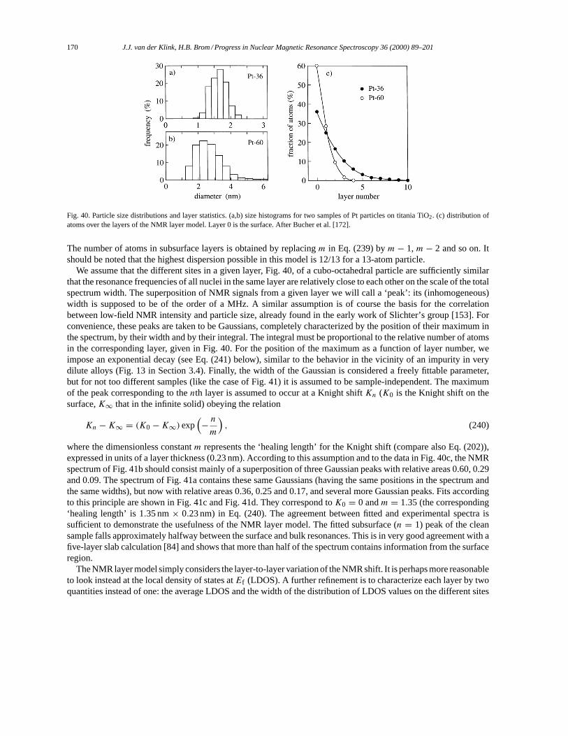
170 J.J. van der Klink, H.B. Brom / Progress in Nuclear Magnetic Resonance Spectroscopy 36 (2000) 89–201
Fig. 40. Particle size distributions and layer statistics. (a,b) size histograms for two samples of Pt particles on titania TiO2. (c) distribution ofatoms over the layers of the NMR layer model. Layer 0 is the surface. After Bucher et al. [172].
The number of atoms in subsurface layers is obtained by replacingm in Eq. (239) bym − 1,m − 2 and so on. Itshould be noted that the highest dispersion possible in this model is 12/13 for a 13-atom particle.
We assume that the different sites in a given layer, Fig. 40, of a cubo-octahedral particle are sufficiently similarthat the resonance frequencies of all nuclei in the same layer are relatively close to each other on the scale of the totalspectrum width. The superposition of NMR signals from a given layer we will call a ‘peak’: its (inhomogeneous)width is supposed to be of the order of a MHz. A similar assumption is of course the basis for the correlationbetween low-field NMR intensity and particle size, already found in the early work of Slichter’s group [153]. Forconvenience, these peaks are taken to be Gaussians, completely characterized by the position of their maximum inthe spectrum, by their width and by their integral. The integral must be proportional to the relative number of atomsin the corresponding layer, given in Fig. 40. For the position of the maximum as a function of layer number, weimpose an exponential decay (see Eq. (241) below), similar to the behavior in the vicinity of an impurity in verydilute alloys (Fig. 13 in Section 3.4). Finally, the width of the Gaussian is considered a freely fittable parameter,but for not too different samples (like the case of Fig. 41) it is assumed to be sample-independent. The maximumof the peak corresponding to thenth layer is assumed to occur at a Knight shiftKn (K0 is the Knight shift on thesurface,K∞ that in the infinite solid) obeying the relation
Kn −K∞ = (K0 −K∞)exp(− nm
), (240)
where the dimensionless constantm represents the ‘healing length’ for the Knight shift (compare also Eq. (202)),expressed in units of a layer thickness (0.23 nm). According to this assumption and to the data in Fig. 40c, the NMRspectrum of Fig. 41b should consist mainly of a superposition of three Gaussian peaks with relative areas 0.60, 0.29and 0.09. The spectrum of Fig. 41a contains these same Gaussians (having the same positions in the spectrum andthe same widths), but now with relative areas 0.36, 0.25 and 0.17, and several more Gaussian peaks. Fits accordingto this principle are shown in Fig. 41c and Fig. 41d. They correspond toK0 = 0 andm = 1.35 (the corresponding‘healing length’ is 1.35 nm× 0.23 nm) in Eq. (240). The agreement between fitted and experimental spectra issufficient to demonstrate the usefulness of the NMR layer model. The fitted subsurface (n = 1) peak of the cleansample falls approximately halfway between the surface and bulk resonances. This is in very good agreement with afive-layer slab calculation [84] and shows that more than half of the spectrum contains information from the surfaceregion.
The NMR layer model simply considers the layer-to-layer variation of the NMR shift. It is perhaps more reasonableto look instead at the local density of states atEf (LDOS). A further refinement is to characterize each layer by twoquantities instead of one: the average LDOS and the width of the distribution of LDOS values on the different sites
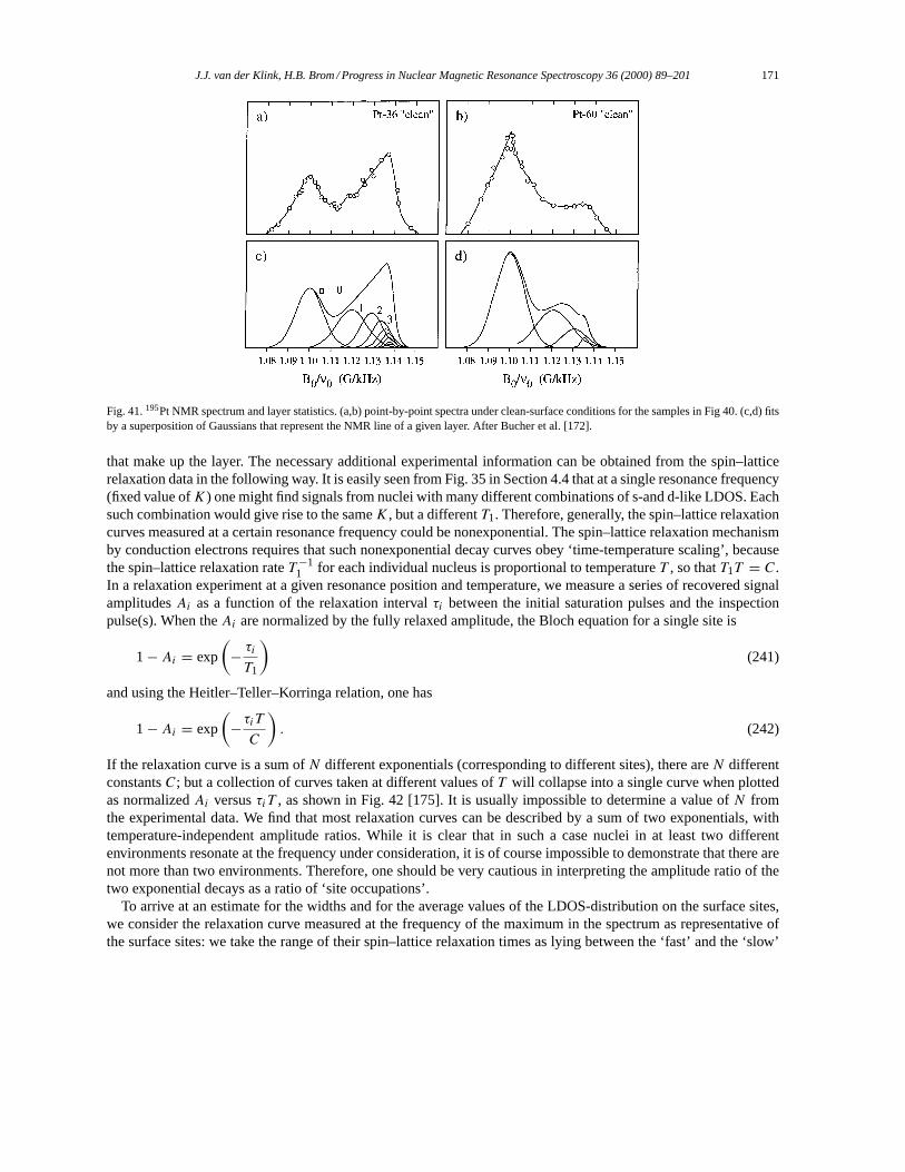
J.J. van der Klink, H.B. Brom / Progress in Nuclear Magnetic Resonance Spectroscopy 36 (2000) 89–201 171
Fig. 41.195Pt NMR spectrum and layer statistics. (a,b) point-by-point spectra under clean-surface conditions for the samples in Fig 40. (c,d) fitsby a superposition of Gaussians that represent the NMR line of a given layer. After Bucher et al. [172].
that make up the layer. The necessary additional experimental information can be obtained from the spin–latticerelaxation data in the following way. It is easily seen from Fig. 35 in Section 4.4 that at a single resonance frequency(fixed value ofK) one might find signals from nuclei with many different combinations of s-and d-like LDOS. Eachsuch combination would give rise to the sameK, but a differentT1. Therefore, generally, the spin–lattice relaxationcurves measured at a certain resonance frequency could be nonexponential. The spin–lattice relaxation mechanismby conduction electrons requires that such nonexponential decay curves obey ‘time-temperature scaling’, becausethe spin–lattice relaxation rateT −1
1 for each individual nucleus is proportional to temperatureT , so thatT1T = C.In a relaxation experiment at a given resonance position and temperature, we measure a series of recovered signalamplitudesAi as a function of the relaxation intervalτi between the initial saturation pulses and the inspectionpulse(s). When theAi are normalized by the fully relaxed amplitude, the Bloch equation for a single site is
1− Ai = exp
(− τiT1
)(241)
and using the Heitler–Teller–Korringa relation, one has
1− Ai = exp
(−τiTC
). (242)
If the relaxation curve is a sum ofN different exponentials (corresponding to different sites), there areN differentconstantsC; but a collection of curves taken at different values ofT will collapse into a single curve when plottedas normalizedAi versusτiT , as shown in Fig. 42 [175]. It is usually impossible to determine a value ofN fromthe experimental data. We find that most relaxation curves can be described by a sum of two exponentials, withtemperature-independent amplitude ratios. While it is clear that in such a case nuclei in at least two differentenvironments resonate at the frequency under consideration, it is of course impossible to demonstrate that there arenot more than two environments. Therefore, one should be very cautious in interpreting the amplitude ratio of thetwo exponential decays as a ratio of ‘site occupations’.
To arrive at an estimate for the widths and for the average values of the LDOS-distribution on the surface sites,we consider the relaxation curve measured at the frequency of the maximum in the spectrum as representative ofthe surface sites: we take the range of their spin–lattice relaxation times as lying between the ‘fast’ and the ‘slow’
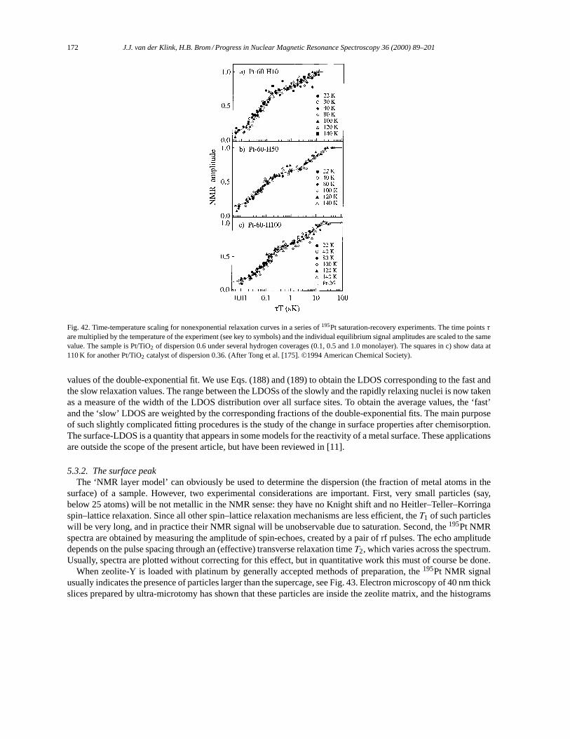
172 J.J. van der Klink, H.B. Brom / Progress in Nuclear Magnetic Resonance Spectroscopy 36 (2000) 89–201
Fig. 42. Time-temperature scaling for nonexponential relaxation curves in a series of195Pt saturation-recovery experiments. The time pointsτ
are multiplied by the temperature of the experiment (see key to symbols) and the individual equilibrium signal amplitudes are scaled to the samevalue. The sample is Pt/TiO2 of dispersion 0.6 under several hydrogen coverages (0.1, 0.5 and 1.0 monolayer). The squares in c) show data at110 K for another Pt/TiO2 catalyst of dispersion 0.36. (After Tong et al. [175]. ©1994 American Chemical Society).
values of the double-exponential fit. We use Eqs. (188) and (189) to obtain the LDOS corresponding to the fast andthe slow relaxation values. The range between the LDOSs of the slowly and the rapidly relaxing nuclei is now takenas a measure of the width of the LDOS distribution over all surface sites. To obtain the average values, the ‘fast’and the ‘slow’ LDOS are weighted by the corresponding fractions of the double-exponential fits. The main purposeof such slightly complicated fitting procedures is the study of the change in surface properties after chemisorption.The surface-LDOS is a quantity that appears in some models for the reactivity of a metal surface. These applicationsare outside the scope of the present article, but have been reviewed in [11].
5.3.2. The surface peakThe ‘NMR layer model’ can obviously be used to determine the dispersion (the fraction of metal atoms in the
surface) of a sample. However, two experimental considerations are important. First, very small particles (say,below 25 atoms) will be not metallic in the NMR sense: they have no Knight shift and no Heitler–Teller–Korringaspin–lattice relaxation. Since all other spin–lattice relaxation mechanisms are less efficient, theT1 of such particleswill be very long, and in practice their NMR signal will be unobservable due to saturation. Second, the195Pt NMRspectra are obtained by measuring the amplitude of spin-echoes, created by a pair of rf pulses. The echo amplitudedepends on the pulse spacing through an (effective) transverse relaxation timeT2, which varies across the spectrum.Usually, spectra are plotted without correcting for this effect, but in quantitative work this must of course be done.
When zeolite-Y is loaded with platinum by generally accepted methods of preparation, the195Pt NMR signalusually indicates the presence of particles larger than the supercage, see Fig. 43. Electron microscopy of 40 nm thickslices prepared by ultra-microtomy has shown that these particles are inside the zeolite matrix, and the histograms
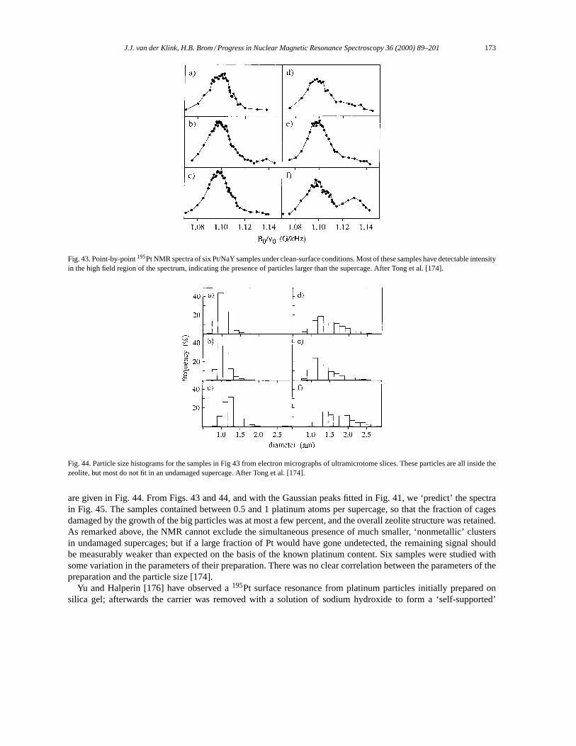
J.J. van der Klink, H.B. Brom / Progress in Nuclear Magnetic Resonance Spectroscopy 36 (2000) 89–201 173
Fig. 43. Point-by-point195Pt NMR spectra of six Pt/NaY samples under clean-surface conditions. Most of these samples have detectable intensityin the high field region of the spectrum, indicating the presence of particles larger than the supercage. After Tong et al. [174].
Fig. 44. Particle size histograms for the samples in Fig 43 from electron micrographs of ultramicrotome slices. These particles are all inside thezeolite, but most do not fit in an undamaged supercage. After Tong et al. [174].
are given in Fig. 44. From Figs. 43 and 44, and with the Gaussian peaks fitted in Fig. 41, we ‘predict’ the spectrain Fig. 45. The samples contained between 0.5 and 1 platinum atoms per supercage, so that the fraction of cagesdamaged by the growth of the big particles was at most a few percent, and the overall zeolite structure was retained.As remarked above, the NMR cannot exclude the simultaneous presence of much smaller, ‘nonmetallic’ clustersin undamaged supercages; but if a large fraction of Pt would have gone undetected, the remaining signal shouldbe measurably weaker than expected on the basis of the known platinum content. Six samples were studied withsome variation in the parameters of their preparation. There was no clear correlation between the parameters of thepreparation and the particle size [174].
Yu and Halperin [176] have observed a195Pt surface resonance from platinum particles initially prepared onsilica gel; afterwards the carrier was removed with a solution of sodium hydroxide to form a ‘self-supported’
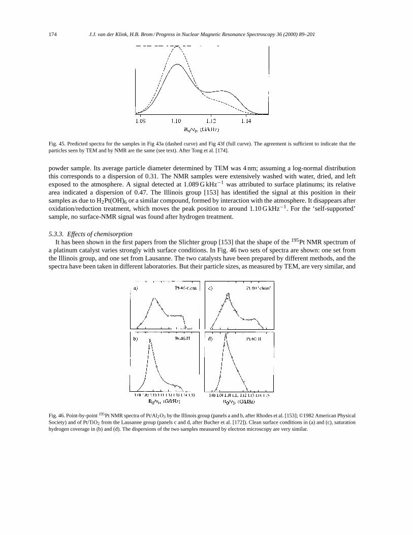
174 J.J. van der Klink, H.B. Brom / Progress in Nuclear Magnetic Resonance Spectroscopy 36 (2000) 89–201
Fig. 45. Predicted spectra for the samples in Fig 43a (dashed curve) and Fig 43f (full curve). The agreement is sufficient to indicate that theparticles seen by TEM and by NMR are the same (see text). After Tong et al. [174].
powder sample. Its average particle diameter determined by TEM was 4 nm; assuming a log-normal distributionthis corresponds to a dispersion of 0.31. The NMR samples were extensively washed with water, dried, and leftexposed to the atmosphere. A signal detected at 1.089 G kHz−1 was attributed to surface platinums; its relativearea indicated a dispersion of 0.47. The Illinois group [153] has identified the signal at this position in theirsamples as due to H2Pt(OH)6 or a similar compound, formed by interaction with the atmosphere. It disappears afteroxidation/reduction treatment, which moves the peak position to around 1.10 G kHz−1. For the ‘self-supported’sample, no surface-NMR signal was found after hydrogen treatment.
5.3.3. Effects of chemisorptionIt has been shown in the first papers from the Slichter group [153] that the shape of the195Pt NMR spectrum of
a platinum catalyst varies strongly with surface conditions. In Fig. 46 two sets of spectra are shown: one set fromthe Illinois group, and one set from Lausanne. The two catalysts have been prepared by different methods, and thespectra have been taken in different laboratories. But their particle sizes, as measured by TEM, are very similar, and
Fig. 46. Point-by-point195Pt NMR spectra of Pt/Al2O3 by the Illinois group (panels a and b, after Rhodes et al. [153]; ©1982 American PhysicalSociety) and of Pt/TiO2 from the Lausanne group (panels c and d, after Bucher et al. [172]). Clean surface conditions in (a) and (c), saturationhydrogen coverage in (b) and (d). The dispersions of the two samples measured by electron microscopy are very similar.
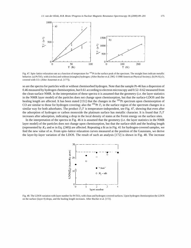
J.J. van der Klink, H.B. Brom / Progress in Nuclear Magnetic Resonance Spectroscopy 36 (2000) 89–201 175
Fig. 47. Spin–lattice relaxation rate as a function of temperature for195Pt in the surface peak of the spectrum. The straight lines indicate metallicbehavior. (a) Pt/TiO2 with (circles) and without (triangles) hydrogen. (After Bucher et al. [90]. ©1988 American Physical Society). (b) Pt/Al2O3
covered with CO. (After Ansermet et al. [177]).
so are the spectra for particles with or without chemisorbed hydrogen. Note that the sample Pt-46 has a dispersion of0.46 measured by hydrogen chemisorption, but 0.61 according to electron microscopy and 0.52–0.62 measured fromthe clean-surface NMR. In the interpretation of these spectra it is assumed that the geometry (i.e. the layer statisticsin the NMR layer model) of the particles does not change upon chemisorption, but that the surface-LDOS and thehealing length are affected. It has been stated [151] that the changes in the195Pt spectrum upon chemisorption ofCO are similar to those for hydrogen covering; also the195PtT1 in the surface region of the spectrum changes in asimilar way for both adsorbates. The productT1T is temperature-independent, see Fig. 47, showing that even afterthe adsorption of hydrogen or carbon monoxide the platinum surface has metallic character. It is found thatT1T
increases after adsorption, indicating a drop in the local density of states at the Fermi energy on the surface sites.In the interpretation of the spectra in Fig. 46 it is assumed that the geometry (i.e. the layer statistics in the NMR
layer model) of the particles does not change upon chemisorption, but that the surface-shift and the healing length(represented byK0 andm in Eq. (240)) are affected. Repeating a fit as in Fig. 41 for hydrogen-covered samples, wefind the new value ofm. From spin–lattice relaxation curves measured at the position of the Gaussians, we derivethe layer-by-layer variation of the LDOS. The result of such an analysis [172] is shown in Fig. 48. The increase
Fig. 48. The LDOS variation with layer number for Pt/TiO2 with clean and hydrogen-covered surfaces. Upon hydrogen chemisorption the LDOSon the surface (layer 0) drops, and the healing length increases. After Bucher et al. [172].
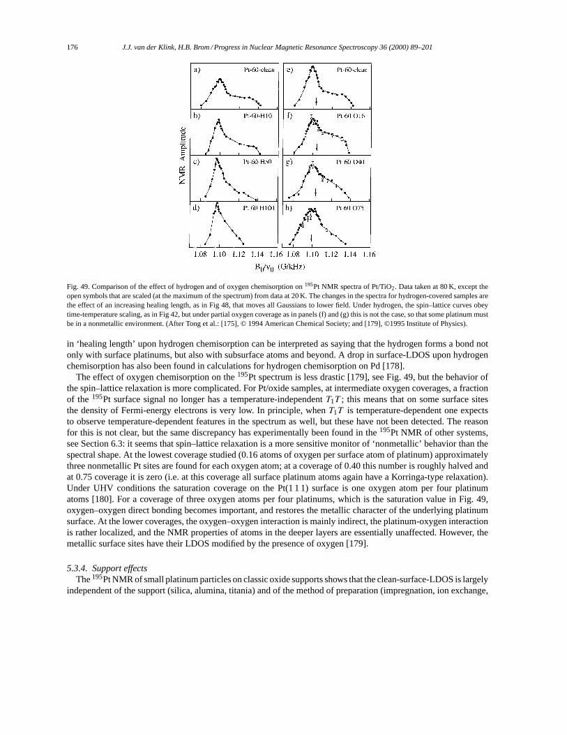
176 J.J. van der Klink, H.B. Brom / Progress in Nuclear Magnetic Resonance Spectroscopy 36 (2000) 89–201
Fig. 49. Comparison of the effect of hydrogen and of oxygen chemisorption on195Pt NMR spectra of Pt/TiO2. Data taken at 80 K, except theopen symbols that are scaled (at the maximum of the spectrum) from data at 20 K. The changes in the spectra for hydrogen-covered samples arethe effect of an increasing healing length, as in Fig 48, that moves all Gaussians to lower field. Under hydrogen, the spin–lattice curves obeytime-temperature scaling, as in Fig 42, but under partial oxygen coverage as in panels (f) and (g) this is not the case, so that some platinum mustbe in a nonmetallic environment. (After Tong et al.: [175], © 1994 American Chemical Society; and [179], ©1995 Institute of Physics).
in ‘healing length’ upon hydrogen chemisorption can be interpreted as saying that the hydrogen forms a bond notonly with surface platinums, but also with subsurface atoms and beyond. A drop in surface-LDOS upon hydrogenchemisorption has also been found in calculations for hydrogen chemisorption on Pd [178].
The effect of oxygen chemisorption on the195Pt spectrum is less drastic [179], see Fig. 49, but the behavior ofthe spin–lattice relaxation is more complicated. For Pt/oxide samples, at intermediate oxygen coverages, a fractionof the 195Pt surface signal no longer has a temperature-independentT1T ; this means that on some surface sitesthe density of Fermi-energy electrons is very low. In principle, whenT1T is temperature-dependent one expectsto observe temperature-dependent features in the spectrum as well, but these have not been detected. The reasonfor this is not clear, but the same discrepancy has experimentally been found in the195Pt NMR of other systems,see Section 6.3: it seems that spin–lattice relaxation is a more sensitive monitor of ‘nonmetallic’ behavior than thespectral shape. At the lowest coverage studied (0.16 atoms of oxygen per surface atom of platinum) approximatelythree nonmetallic Pt sites are found for each oxygen atom; at a coverage of 0.40 this number is roughly halved andat 0.75 coverage it is zero (i.e. at this coverage all surface platinum atoms again have a Korringa-type relaxation).Under UHV conditions the saturation coverage on the Pt(1 1 1) surface is one oxygen atom per four platinumatoms [180]. For a coverage of three oxygen atoms per four platinums, which is the saturation value in Fig. 49,oxygen–oxygen direct bonding becomes important, and restores the metallic character of the underlying platinumsurface. At the lower coverages, the oxygen–oxygen interaction is mainly indirect, the platinum-oxygen interactionis rather localized, and the NMR properties of atoms in the deeper layers are essentially unaffected. However, themetallic surface sites have their LDOS modified by the presence of oxygen [179].
5.3.4. Support effectsThe195Pt NMR of small platinum particles on classic oxide supports shows that the clean-surface-LDOS is largely
independent of the support (silica, alumina, titania) and of the method of preparation (impregnation, ion exchange,
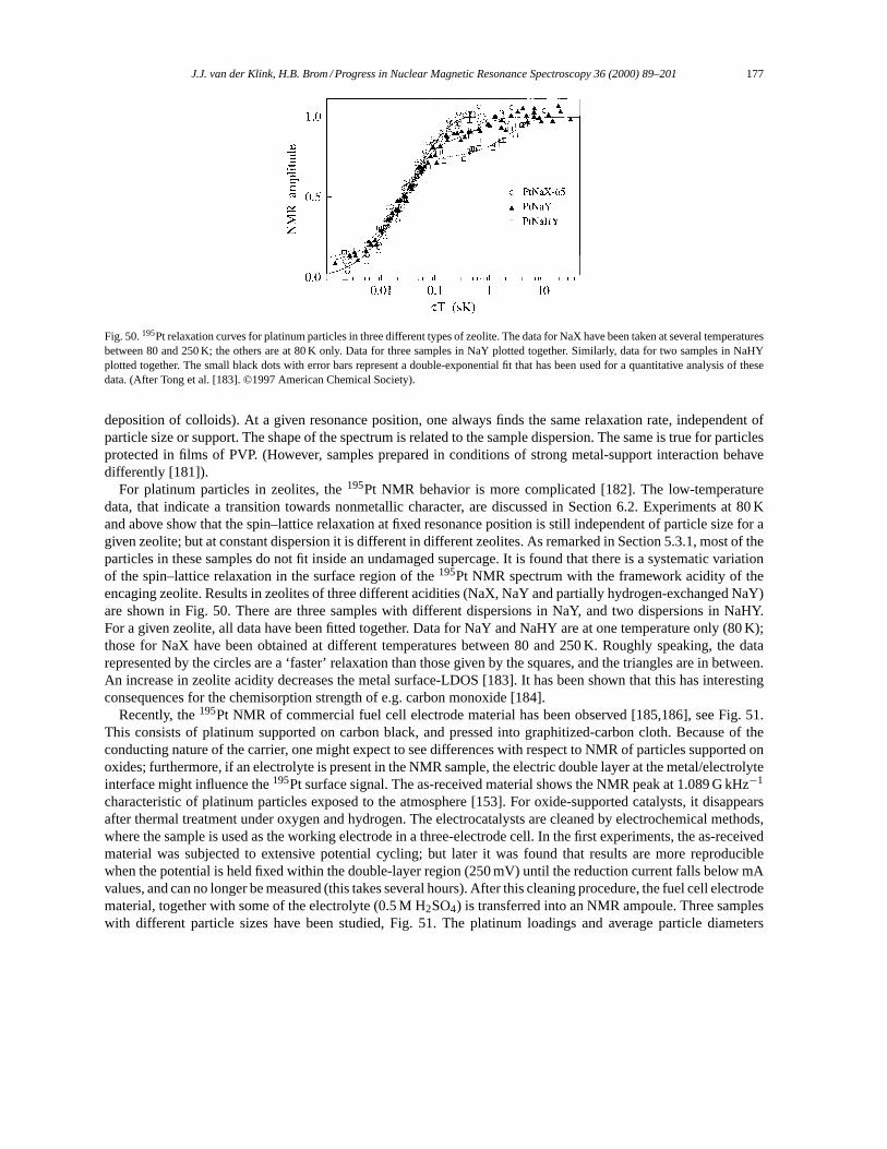
J.J. van der Klink, H.B. Brom / Progress in Nuclear Magnetic Resonance Spectroscopy 36 (2000) 89–201 177
Fig. 50.195Pt relaxation curves for platinum particles in three different types of zeolite. The data for NaX have been taken at several temperaturesbetween 80 and 250 K; the others are at 80 K only. Data for three samples in NaY plotted together. Similarly, data for two samples in NaHYplotted together. The small black dots with error bars represent a double-exponential fit that has been used for a quantitative analysis of thesedata. (After Tong et al. [183]. ©1997 American Chemical Society).
deposition of colloids). At a given resonance position, one always finds the same relaxation rate, independent ofparticle size or support. The shape of the spectrum is related to the sample dispersion. The same is true for particlesprotected in films of PVP. (However, samples prepared in conditions of strong metal-support interaction behavedifferently [181]).
For platinum particles in zeolites, the195Pt NMR behavior is more complicated [182]. The low-temperaturedata, that indicate a transition towards nonmetallic character, are discussed in Section 6.2. Experiments at 80 Kand above show that the spin–lattice relaxation at fixed resonance position is still independent of particle size for agiven zeolite; but at constant dispersion it is different in different zeolites. As remarked in Section 5.3.1, most of theparticles in these samples do not fit inside an undamaged supercage. It is found that there is a systematic variationof the spin–lattice relaxation in the surface region of the195Pt NMR spectrum with the framework acidity of theencaging zeolite. Results in zeolites of three different acidities (NaX, NaY and partially hydrogen-exchanged NaY)are shown in Fig. 50. There are three samples with different dispersions in NaY, and two dispersions in NaHY.For a given zeolite, all data have been fitted together. Data for NaY and NaHY are at one temperature only (80 K);those for NaX have been obtained at different temperatures between 80 and 250 K. Roughly speaking, the datarepresented by the circles are a ‘faster’ relaxation than those given by the squares, and the triangles are in between.An increase in zeolite acidity decreases the metal surface-LDOS [183]. It has been shown that this has interestingconsequences for the chemisorption strength of e.g. carbon monoxide [184].
Recently, the195Pt NMR of commercial fuel cell electrode material has been observed [185,186], see Fig. 51.This consists of platinum supported on carbon black, and pressed into graphitized-carbon cloth. Because of theconducting nature of the carrier, one might expect to see differences with respect to NMR of particles supported onoxides; furthermore, if an electrolyte is present in the NMR sample, the electric double layer at the metal/electrolyteinterface might influence the195Pt surface signal. The as-received material shows the NMR peak at 1.089 G kHz−1
characteristic of platinum particles exposed to the atmosphere [153]. For oxide-supported catalysts, it disappearsafter thermal treatment under oxygen and hydrogen. The electrocatalysts are cleaned by electrochemical methods,where the sample is used as the working electrode in a three-electrode cell. In the first experiments, the as-receivedmaterial was subjected to extensive potential cycling; but later it was found that results are more reproduciblewhen the potential is held fixed within the double-layer region (250 mV) until the reduction current falls below mAvalues, and can no longer be measured (this takes several hours). After this cleaning procedure, the fuel cell electrodematerial, together with some of the electrolyte (0.5 M H2SO4) is transferred into an NMR ampoule. Three sampleswith different particle sizes have been studied, Fig. 51. The platinum loadings and average particle diameters
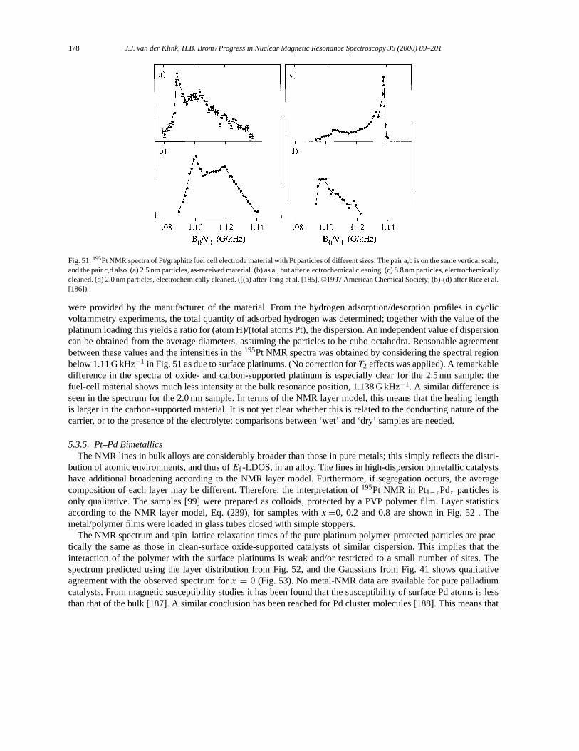
178 J.J. van der Klink, H.B. Brom / Progress in Nuclear Magnetic Resonance Spectroscopy 36 (2000) 89–201
Fig. 51.195Pt NMR spectra of Pt/graphite fuel cell electrode material with Pt particles of different sizes. The pair a,b is on the same vertical scale,and the pair c,d also. (a) 2.5 nm particles, as-received material. (b) as a., but after electrochemical cleaning. (c) 8.8 nm particles, electrochemicallycleaned. (d) 2.0 nm particles, electrochemically cleaned. ([(a) after Tong et al. [185], ©1997 American Chemical Society; (b)-(d) after Rice et al.[186]).
were provided by the manufacturer of the material. From the hydrogen adsorption/desorption profiles in cyclicvoltammetry experiments, the total quantity of adsorbed hydrogen was determined; together with the value of theplatinum loading this yields a ratio for (atom H)/(total atoms Pt), the dispersion. An independent value of dispersioncan be obtained from the average diameters, assuming the particles to be cubo-octahedra. Reasonable agreementbetween these values and the intensities in the195Pt NMR spectra was obtained by considering the spectral regionbelow 1.11 G kHz−1 in Fig. 51 as due to surface platinums. (No correction forT2 effects was applied). A remarkabledifference in the spectra of oxide- and carbon-supported platinum is especially clear for the 2.5 nm sample: thefuel-cell material shows much less intensity at the bulk resonance position, 1.138 G kHz−1. A similar difference isseen in the spectrum for the 2.0 nm sample. In terms of the NMR layer model, this means that the healing lengthis larger in the carbon-supported material. It is not yet clear whether this is related to the conducting nature of thecarrier, or to the presence of the electrolyte: comparisons between ‘wet’ and ‘dry’ samples are needed.
5.3.5. Pt–Pd BimetallicsThe NMR lines in bulk alloys are considerably broader than those in pure metals; this simply reflects the distri-
bution of atomic environments, and thus ofEf -LDOS, in an alloy. The lines in high-dispersion bimetallic catalystshave additional broadening according to the NMR layer model. Furthermore, if segregation occurs, the averagecomposition of each layer may be different. Therefore, the interpretation of195Pt NMR in Pt1−xPdx particles isonly qualitative. The samples [99] were prepared as colloids, protected by a PVP polymer film. Layer statisticsaccording to the NMR layer model, Eq. (239), for samples withx=0, 0.2 and 0.8 are shown in Fig. 52 . Themetal/polymer films were loaded in glass tubes closed with simple stoppers.
The NMR spectrum and spin–lattice relaxation times of the pure platinum polymer-protected particles are prac-tically the same as those in clean-surface oxide-supported catalysts of similar dispersion. This implies that theinteraction of the polymer with the surface platinums is weak and/or restricted to a small number of sites. Thespectrum predicted using the layer distribution from Fig. 52, and the Gaussians from Fig. 41 shows qualitativeagreement with the observed spectrum forx = 0 (Fig. 53). No metal-NMR data are available for pure palladiumcatalysts. From magnetic susceptibility studies it has been found that the susceptibility of surface Pd atoms is lessthan that of the bulk [187]. A similar conclusion has been reached for Pd cluster molecules [188]. This means that
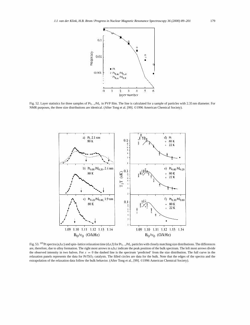
J.J. van der Klink, H.B. Brom / Progress in Nuclear Magnetic Resonance Spectroscopy 36 (2000) 89–201 179
Fig. 52. Layer statistics for three samples of Pt1−xPdx in PVP film. The line is calculated for a sample of particles with 2.35 nm diameter. ForNMR purposes, the three size distributions are identical. (After Tong et al. [99]. ©1996 American Chemical Society).
Fig. 53.195Pt spectra (a,b,c) and spin–lattice relaxation time (d,e,f) for Pt1−xPdx particles with closely matching size distributions. The differencesare, therefore, due to alloy formation. The right most arrows in a,b,c indicate the peak position of the bulk spectrum. The left most arrows dividethe observed intensity in two halves. Forx = 0 the dashed line is the spectrum ‘predicted’ from the size distribution. The full curve in therelaxation panels represents the data for Pt/TiO2 catalysts. The filled circles are data for the bulk. Note that the edges of the spectra and theextrapolation of the relaxation data follow the bulk behavior. (After Tong et al., [99]. ©1996 American Chemical Society).
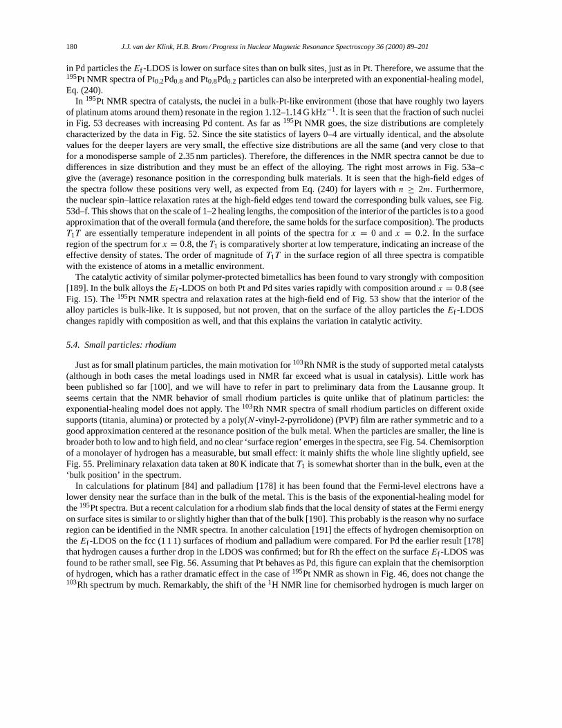
180 J.J. van der Klink, H.B. Brom / Progress in Nuclear Magnetic Resonance Spectroscopy 36 (2000) 89–201
in Pd particles theEf -LDOS is lower on surface sites than on bulk sites, just as in Pt. Therefore, we assume that the195Pt NMR spectra of Pt0.2Pd0.8 and Pt0.8Pd0.2 particles can also be interpreted with an exponential-healing model,Eq. (240).
In 195Pt NMR spectra of catalysts, the nuclei in a bulk-Pt-like environment (those that have roughly two layersof platinum atoms around them) resonate in the region 1.12–1.14 G kHz−1. It is seen that the fraction of such nucleiin Fig. 53 decreases with increasing Pd content. As far as195Pt NMR goes, the size distributions are completelycharacterized by the data in Fig. 52. Since the site statistics of layers 0–4 are virtually identical, and the absolutevalues for the deeper layers are very small, the effective size distributions are all the same (and very close to thatfor a monodisperse sample of 2.35 nm particles). Therefore, the differences in the NMR spectra cannot be due todifferences in size distribution and they must be an effect of the alloying. The right most arrows in Fig. 53a–cgive the (average) resonance position in the corresponding bulk materials. It is seen that the high-field edges ofthe spectra follow these positions very well, as expected from Eq. (240) for layers withn ≥ 2m. Furthermore,the nuclear spin–lattice relaxation rates at the high-field edges tend toward the corresponding bulk values, see Fig.53d–f. This shows that on the scale of 1–2 healing lengths, the composition of the interior of the particles is to a goodapproximation that of the overall formula (and therefore, the same holds for the surface composition). The productsT1T are essentially temperature independent in all points of the spectra forx = 0 andx = 0.2. In the surfaceregion of the spectrum forx = 0.8, theT1 is comparatively shorter at low temperature, indicating an increase of theeffective density of states. The order of magnitude ofT1T in the surface region of all three spectra is compatiblewith the existence of atoms in a metallic environment.
The catalytic activity of similar polymer-protected bimetallics has been found to vary strongly with composition[189]. In the bulk alloys theEf -LDOS on both Pt and Pd sites varies rapidly with composition aroundx = 0.8 (seeFig. 15). The195Pt NMR spectra and relaxation rates at the high-field end of Fig. 53 show that the interior of thealloy particles is bulk-like. It is supposed, but not proven, that on the surface of the alloy particles theEf -LDOSchanges rapidly with composition as well, and that this explains the variation in catalytic activity.
5.4. Small particles: rhodium
Just as for small platinum particles, the main motivation for103Rh NMR is the study of supported metal catalysts(although in both cases the metal loadings used in NMR far exceed what is usual in catalysis). Little work hasbeen published so far [100], and we will have to refer in part to preliminary data from the Lausanne group. Itseems certain that the NMR behavior of small rhodium particles is quite unlike that of platinum particles: theexponential-healing model does not apply. The103Rh NMR spectra of small rhodium particles on different oxidesupports (titania, alumina) or protected by a poly(N -vinyl-2-pyrrolidone) (PVP) film are rather symmetric and to agood approximation centered at the resonance position of the bulk metal. When the particles are smaller, the line isbroader both to low and to high field, and no clear ‘surface region’ emerges in the spectra, see Fig. 54. Chemisorptionof a monolayer of hydrogen has a measurable, but small effect: it mainly shifts the whole line slightly upfield, seeFig. 55. Preliminary relaxation data taken at 80 K indicate thatT1 is somewhat shorter than in the bulk, even at the‘bulk position’ in the spectrum.
In calculations for platinum [84] and palladium [178] it has been found that the Fermi-level electrons have alower density near the surface than in the bulk of the metal. This is the basis of the exponential-healing model forthe195Pt spectra. But a recent calculation for a rhodium slab finds that the local density of states at the Fermi energyon surface sites is similar to or slightly higher than that of the bulk [190]. This probably is the reason why no surfaceregion can be identified in the NMR spectra. In another calculation [191] the effects of hydrogen chemisorption ontheEf -LDOS on the fcc (1 1 1) surfaces of rhodium and palladium were compared. For Pd the earlier result [178]that hydrogen causes a further drop in the LDOS was confirmed; but for Rh the effect on the surfaceEf -LDOS wasfound to be rather small, see Fig. 56. Assuming that Pt behaves as Pd, this figure can explain that the chemisorptionof hydrogen, which has a rather dramatic effect in the case of195Pt NMR as shown in Fig. 46, does not change the103Rh spectrum by much. Remarkably, the shift of the1H NMR line for chemisorbed hydrogen is much larger on
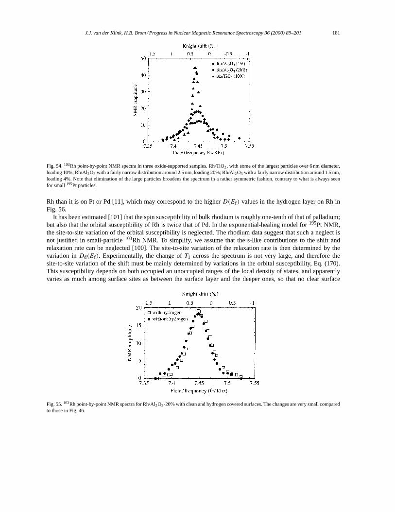
J.J. van der Klink, H.B. Brom / Progress in Nuclear Magnetic Resonance Spectroscopy 36 (2000) 89–201 181
Fig. 54.103Rh point-by-point NMR spectra in three oxide-supported samples. Rh/TiO2, with some of the largest particles over 6 nm diameter,loading 10%; Rh/Al2O3 with a fairly narrow distribution around 2.5 nm, loading 20%; Rh/Al2O3 with a fairly narrow distribution around 1.5 nm,loading 4%. Note that elimination of the large particles broadens the spectrum in a rather symmetric fashion, contrary to what is always seenfor small195Pt particles.
Rh than it is on Pt or Pd [11], which may correspond to the higherD(Ef ) values in the hydrogen layer on Rh inFig. 56.
It has been estimated [101] that the spin susceptibility of bulk rhodium is roughly one-tenth of that of palladium;but also that the orbital susceptibility of Rh is twice that of Pd. In the exponential-healing model for195Pt NMR,the site-to-site variation of the orbital susceptibility is neglected. The rhodium data suggest that such a neglect isnot justified in small-particle103Rh NMR. To simplify, we assume that the s-like contributions to the shift andrelaxation rate can be neglected [100]. The site-to-site variation of the relaxation rate is then determined by thevariation inDd(Ef ). Experimentally, the change ofT1 across the spectrum is not very large, and therefore thesite-to-site variation of the shift must be mainly determined by variations in the orbital susceptibility, Eq. (170).This susceptibility depends on both occupied an unoccupied ranges of the local density of states, and apparentlyvaries as much among surface sites as between the surface layer and the deeper ones, so that no clear surface
Fig. 55.103Rh point-by-point NMR spectra for Rh/Al2O3-20% with clean and hydrogen covered surfaces. The changes are very small comparedto those in Fig. 46.
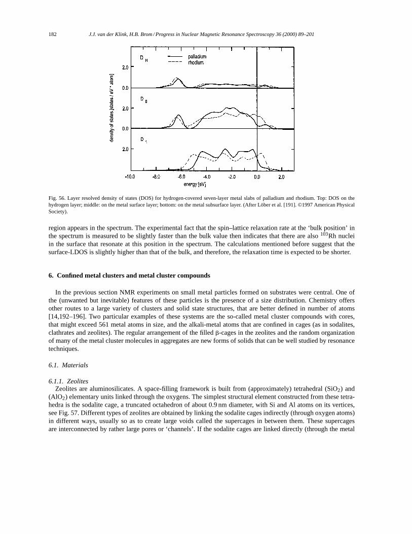
182 J.J. van der Klink, H.B. Brom / Progress in Nuclear Magnetic Resonance Spectroscopy 36 (2000) 89–201
Fig. 56. Layer resolved density of states (DOS) for hydrogen-covered seven-layer metal slabs of palladium and rhodium. Top: DOS on thehydrogen layer; middle: on the metal surface layer; bottom: on the metal subsurface layer. (After Löber et al. [191]. ©1997 American PhysicalSociety).
region appears in the spectrum. The experimental fact that the spin–lattice relaxation rate at the ‘bulk position’ inthe spectrum is measured to be slightly faster than the bulk value then indicates that there are also103Rh nucleiin the surface that resonate at this position in the spectrum. The calculations mentioned before suggest that thesurface-LDOS is slightly higher than that of the bulk, and therefore, the relaxation time is expected to be shorter.
6. Confined metal clusters and metal cluster compounds
In the previous section NMR experiments on small metal particles formed on substrates were central. One ofthe (unwanted but inevitable) features of these particles is the presence of a size distribution. Chemistry offersother routes to a large variety of clusters and solid state structures, that are better defined in number of atoms[14,192–196]. Two particular examples of these systems are the so-called metal cluster compounds with cores,that might exceed 561 metal atoms in size, and the alkali-metal atoms that are confined in cages (as in sodalites,clathrates and zeolites). The regular arrangement of the filledb-cages in the zeolites and the random organizationof many of the metal cluster molecules in aggregates are new forms of solids that can be well studied by resonancetechniques.
6.1. Materials
6.1.1. ZeolitesZeolites are aluminosilicates. A space-filling framework is built from (approximately) tetrahedral (SiO2) and
(AlO2) elementary units linked through the oxygens. The simplest structural element constructed from these tetra-hedra is the sodalite cage, a truncated octahedron of about 0.9 nm diameter, with Si and Al atoms on its vertices,see Fig. 57. Different types of zeolites are obtained by linking the sodalite cages indirectly (through oxygen atoms)in different ways, usually so as to create large voids called the supercages in between them. These supercagesare interconnected by rather large pores or ‘channels’. If the sodalite cages are linked directly (through the metal
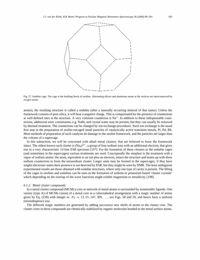
J.J. van der Klink, H.B. Brom / Progress in Nuclear Magnetic Resonance Spectroscopy 36 (2000) 89–201 183
Fig. 57. Sodalite cage. The cage is the building block of zeolites. Alternating silicon and aluminum atoms at the vertices are interconnected byoxygen atoms.
atoms), the resulting structure is called a sodalite (after a naturally occurring mineral of that name). Unless theframework consists of pure silica, it will bear a negative charge. This is compensated by the presence of counterionsat well-defined sites in the structure. A very common counterion is Na+. In addition to these indispensable coun-terions, additional ionic constituents, e.g. NaBr, and crystal water may be present, but they can usually be removedby thermal treatment. The counterions can be changed by ion-exchange procedures. Such ion exchange is the usualfirst step in the preparation of zeolite-encaged small particles of catalytically active transition metals, Pt, Pd, Rh.Most methods of preparation of such catalysts do damage to the zeolite framework, and the particles are larger thanthe volume of a supercage.
In this subsection, we will be concerned with alkali metal clusters, that are believed to leave the frameworkintact. The oldest known such cluster is (Na4)3+, a group of four sodium ions with an additional electron, that givesrise to a very characteristic 13-line ESR spectrum [197]. For the formation of these clusters in the sodalite cages(and sometimes in the supercages) various treatments are used. Conceptually the simplest is the treatment with avapor of sodium atoms: the atom, equivalent to an ion plus an electron, enters the structure and teams up with threesodium counterions to form the tetrasodium cluster. Larger units may be formed in the supercages; if they havesinglet electronic states their presence is not detected by ESR, but they might be seen by NMR. The least ambiguousexperimental results are those obtained with sodalite structures, where only one type of cavity is present. The fillingof the cages in zeolites and sodalites can be seen as the formation of sodium-or potassium based ‘cluster crystals’which depending on the overlap of the wave functions might exhibit magnetism or metallicity [198].
6.1.2. Metal cluster compoundsIn a metal cluster compound (MCM) a core or network of metal atoms is surrounded by nonmetallic ligands. One
variety (type A) of MCMs consist of a metal core in a cuboctahedral arrangement with a magic number of atomsgiven by Eq. (238) with integerm: NT = 13,55,147,309, . . . , see Figs. 58 and 59, and hence have a uniform(monodisperse) size.
The different magic numbers are generated by adding successive new shells of atoms to the cluster core. Thecluster cores in these compounds are chemically stabilized by organic molecules bonded to the metal surface atoms.
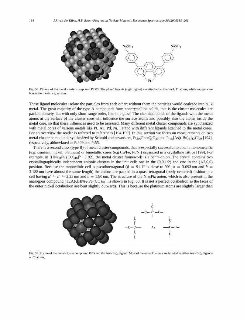
184 J.J. van der Klink, H.B. Brom / Progress in Nuclear Magnetic Resonance Spectroscopy 36 (2000) 89–201
Fig. 58. Pt core of the metal cluster compound Pt309. The phen∗ ligands (right figure) are attached to the black Pt atoms, while oxygens arebonded to the dark gray sites.
These ligand molecules isolate the particles from each other; without them the particles would coalesce into bulkmetal. The great majority of the type A compounds form noncrystalline solids, that is the cluster molecules arepacked densely, but with only short-range order, like in a glass. The chemical bonds of the ligands with the metalatoms at the surface of the cluster core will influence the surface atoms and possibly also the atoms inside themetal core, so that these influences need to be assessed. Many different metal cluster compounds are synthesizedwith metal cores of various metals like Pt, Au, Pd, Ni, Fe and with different ligands attached to the metal cores.For an overview the reader is referred to references [194,199]. In this section we focus on measurements on twometal cluster compounds synthesized by Schmid and coworkers, Pt309Phen∗36O30 and Pt55[As(t-Bu)3]12Cl20 [194],respectively, abbreviated as Pt309 and Pt55.
There is a second class (type B) of metal cluster compounds, that is especially successful to obtain monometallic(e.g. osmium, nickel, platinum) or bimetallic cores (e.g Cu/Fe, Pt/Ni) organized in a crystalline lattice [199]. Forexample, in [HNi38Pt6(CO)48]5− [192], the metal cluster framework is a penta-anion. The crystal contains twocrystallographically independent anionic clusters in the unit cell: one in the (0,0,1/2) and one in the (1/2,0,0)position. Because the monoclinic cell is pseudotetragonal (β = 91.1◦ is close to 90◦; a = 3.093 nm andb =3.188 nm have almost the same length) the anions are packed in a quasi-tetragonal (body centered) fashion in acell havinga′ ≈ b′ ≈ 2.23 nm andc = 1.90 nm. The structure of the Ni38Pt6 anion, which is also present in theanalogous compound (TEA)5[HNi38Pt6(CO)48], is shown in Fig. 60. It is not a perfect octahedron as the faces ofthe outer nickel octahedron are bent slightly outwards. This is because the platinum atoms are slightly larger than
Fig. 59. Pt core of the metal cluster compound Pt55 and the As(t-Bu)3 ligand. Most of the outer Pt atoms are bonded to either As(t-Bu)3 ligandsor Cl atoms.
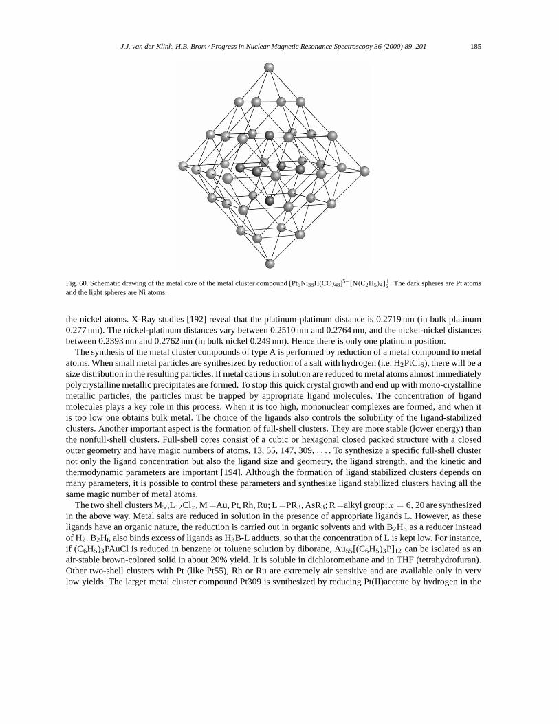
J.J. van der Klink, H.B. Brom / Progress in Nuclear Magnetic Resonance Spectroscopy 36 (2000) 89–201 185
Fig. 60. Schematic drawing of the metal core of the metal cluster compound [Pt6Ni38H(CO)48]5−[N(C2H5)4]+5 . The dark spheres are Pt atomsand the light spheres are Ni atoms.
the nickel atoms. X-Ray studies [192] reveal that the platinum-platinum distance is 0.2719 nm (in bulk platinum0.277 nm). The nickel-platinum distances vary between 0.2510 nm and 0.2764 nm, and the nickel-nickel distancesbetween 0.2393 nm and 0.2762 nm (in bulk nickel 0.249 nm). Hence there is only one platinum position.
The synthesis of the metal cluster compounds of type A is performed by reduction of a metal compound to metalatoms. When small metal particles are synthesized by reduction of a salt with hydrogen (i.e. H2PtCl6), there will be asize distribution in the resulting particles. If metal cations in solution are reduced to metal atoms almost immediatelypolycrystalline metallic precipitates are formed. To stop this quick crystal growth and end up with mono-crystallinemetallic particles, the particles must be trapped by appropriate ligand molecules. The concentration of ligandmolecules plays a key role in this process. When it is too high, mononuclear complexes are formed, and when itis too low one obtains bulk metal. The choice of the ligands also controls the solubility of the ligand-stabilizedclusters. Another important aspect is the formation of full-shell clusters. They are more stable (lower energy) thanthe nonfull-shell clusters. Full-shell cores consist of a cubic or hexagonal closed packed structure with a closedouter geometry and have magic numbers of atoms, 13, 55, 147, 309,. . . . To synthesize a specific full-shell clusternot only the ligand concentration but also the ligand size and geometry, the ligand strength, and the kinetic andthermodynamic parameters are important [194]. Although the formation of ligand stabilized clusters depends onmany parameters, it is possible to control these parameters and synthesize ligand stabilized clusters having all thesame magic number of metal atoms.
The two shell clusters M55L12Clx , M=Au, Pt, Rh, Ru; L=PR3, AsR3; R=alkyl group;x = 6,20 are synthesizedin the above way. Metal salts are reduced in solution in the presence of appropriate ligands L. However, as theseligands have an organic nature, the reduction is carried out in organic solvents and with B2H6 as a reducer insteadof H2. B2H6 also binds excess of ligands as H3B-L adducts, so that the concentration of L is kept low. For instance,if (C6H5)3PAuCl is reduced in benzene or toluene solution by diborane, Au55[(C6H5)3P]12 can be isolated as anair-stable brown-colored solid in about 20% yield. It is soluble in dichloromethane and in THF (tetrahydrofuran).Other two-shell clusters with Pt (like Pt55), Rh or Ru are extremely air sensitive and are available only in verylow yields. The larger metal cluster compound Pt309 is synthesized by reducing Pt(II)acetate by hydrogen in the
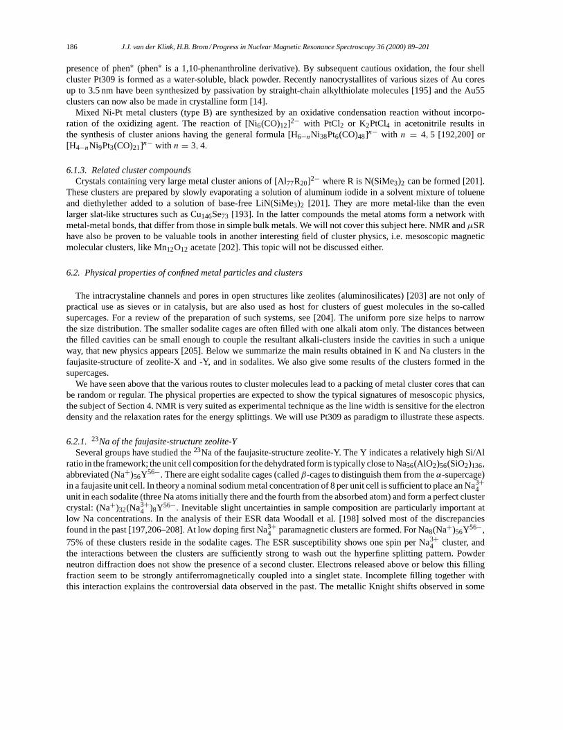
186 J.J. van der Klink, H.B. Brom / Progress in Nuclear Magnetic Resonance Spectroscopy 36 (2000) 89–201
presence of phen∗ (phen∗ is a 1,10-phenanthroline derivative). By subsequent cautious oxidation, the four shellcluster Pt309 is formed as a water-soluble, black powder. Recently nanocrystallites of various sizes of Au coresup to 3.5 nm have been synthesized by passivation by straight-chain alkylthiolate molecules [195] and the Au55clusters can now also be made in crystalline form [14].
Mixed Ni-Pt metal clusters (type B) are synthesized by an oxidative condensation reaction without incorpo-ration of the oxidizing agent. The reaction of [Ni6(CO)12]2− with PtCl2 or K2PtCl4 in acetonitrile results inthe synthesis of cluster anions having the general formula [H6−nNi38Pt6(CO)48]n− with n = 4,5 [192,200] or[H4−nNi9Pt3(CO)21]n− with n = 3,4.
6.1.3. Related cluster compoundsCrystals containing very large metal cluster anions of [Al77R20]2− where R is N(SiMe3)2 can be formed [201].
These clusters are prepared by slowly evaporating a solution of aluminum iodide in a solvent mixture of tolueneand diethylether added to a solution of base-free LiN(SiMe3)2 [201]. They are more metal-like than the evenlarger slat-like structures such as Cu146Se73 [193]. In the latter compounds the metal atoms form a network withmetal-metal bonds, that differ from those in simple bulk metals. We will not cover this subject here. NMR andµSRhave also be proven to be valuable tools in another interesting field of cluster physics, i.e. mesoscopic magneticmolecular clusters, like Mn12O12 acetate [202]. This topic will not be discussed either.
6.2. Physical properties of confined metal particles and clusters
The intracrystaline channels and pores in open structures like zeolites (aluminosilicates) [203] are not only ofpractical use as sieves or in catalysis, but are also used as host for clusters of guest molecules in the so-calledsupercages. For a review of the preparation of such systems, see [204]. The uniform pore size helps to narrowthe size distribution. The smaller sodalite cages are often filled with one alkali atom only. The distances betweenthe filled cavities can be small enough to couple the resultant alkali-clusters inside the cavities in such a uniqueway, that new physics appears [205]. Below we summarize the main results obtained in K and Na clusters in thefaujasite-structure of zeolite-X and -Y, and in sodalites. We also give some results of the clusters formed in thesupercages.
We have seen above that the various routes to cluster molecules lead to a packing of metal cluster cores that canbe random or regular. The physical properties are expected to show the typical signatures of mesoscopic physics,the subject of Section 4. NMR is very suited as experimental technique as the line width is sensitive for the electrondensity and the relaxation rates for the energy splittings. We will use Pt309 as paradigm to illustrate these aspects.
6.2.1. 23Na of the faujasite-structure zeolite-YSeveral groups have studied the23Na of the faujasite-structure zeolite-Y. The Y indicates a relatively high Si/Al
ratio in the framework; the unit cell composition for the dehydrated form is typically close to Na56(AlO2)56(SiO2)136,abbreviated (Na+)56Y56−. There are eight sodalite cages (calledβ-cages to distinguish them from theα-supercage)in a faujasite unit cell. In theory a nominal sodium metal concentration of 8 per unit cell is sufficient to place an Na3+
4unit in each sodalite (three Na atoms initially there and the fourth from the absorbed atom) and form a perfect clustercrystal: (Na+)32(Na3+
4 )8Y56−. Inevitable slight uncertainties in sample composition are particularly important atlow Na concentrations. In the analysis of their ESR data Woodall et al. [198] solved most of the discrepanciesfound in the past [197,206–208]. At low doping first Na3+
4 paramagnetic clusters are formed. For Na8(Na+)56Y56−,75% of these clusters reside in the sodalite cages. The ESR susceptibility shows one spin per Na3+
4 cluster, andthe interactions between the clusters are sufficiently strong to wash out the hyperfine splitting pattern. Powderneutron diffraction does not show the presence of a second cluster. Electrons released above or below this fillingfraction seem to be strongly antiferromagnetically coupled into a singlet state. Incomplete filling together withthis interaction explains the controversial data observed in the past. The metallic Knight shifts observed in some
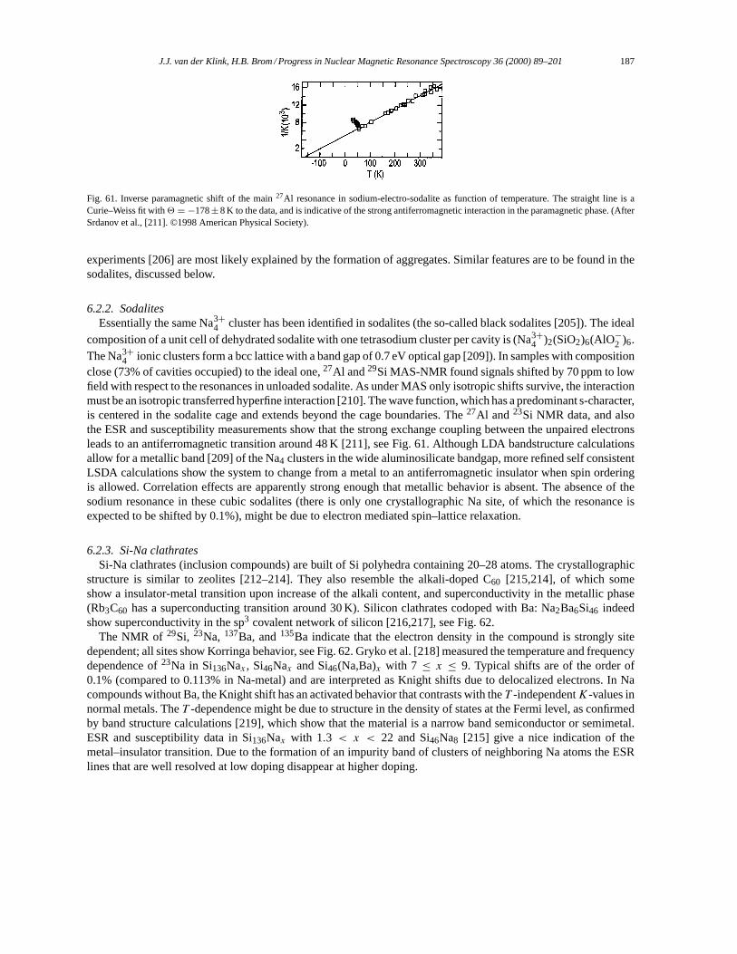
J.J. van der Klink, H.B. Brom / Progress in Nuclear Magnetic Resonance Spectroscopy 36 (2000) 89–201 187
Fig. 61. Inverse paramagnetic shift of the main27Al resonance in sodium-electro-sodalite as function of temperature. The straight line is aCurie–Weiss fit with2 = −178±8 K to the data, and is indicative of the strong antiferromagnetic interaction in the paramagnetic phase. (AfterSrdanov et al., [211]. ©1998 American Physical Society).
experiments [206] are most likely explained by the formation of aggregates. Similar features are to be found in thesodalites, discussed below.
6.2.2. SodalitesEssentially the same Na3+
4 cluster has been identified in sodalites (the so-called black sodalites [205]). The idealcomposition of a unit cell of dehydrated sodalite with one tetrasodium cluster per cavity is (Na3+
4 )2(SiO2)6(AlO−2 )6.The Na3+4 ionic clusters form a bcc lattice with a band gap of 0.7 eV optical gap [209]). In samples with compositionclose (73% of cavities occupied) to the ideal one,27Al and29Si MAS-NMR found signals shifted by 70 ppm to lowfield with respect to the resonances in unloaded sodalite. As under MAS only isotropic shifts survive, the interactionmust be an isotropic transferred hyperfine interaction [210]. The wave function, which has a predominant s-character,is centered in the sodalite cage and extends beyond the cage boundaries. The27Al and 23Si NMR data, and alsothe ESR and susceptibility measurements show that the strong exchange coupling between the unpaired electronsleads to an antiferromagnetic transition around 48 K [211], see Fig. 61. Although LDA bandstructure calculationsallow for a metallic band [209] of the Na4 clusters in the wide aluminosilicate bandgap, more refined self consistentLSDA calculations show the system to change from a metal to an antiferromagnetic insulator when spin orderingis allowed. Correlation effects are apparently strong enough that metallic behavior is absent. The absence of thesodium resonance in these cubic sodalites (there is only one crystallographic Na site, of which the resonance isexpected to be shifted by 0.1%), might be due to electron mediated spin–lattice relaxation.
6.2.3. Si-Na clathratesSi-Na clathrates (inclusion compounds) are built of Si polyhedra containing 20–28 atoms. The crystallographic
structure is similar to zeolites [212–214]. They also resemble the alkali-doped C60 [215,214], of which someshow a insulator-metal transition upon increase of the alkali content, and superconductivity in the metallic phase(Rb3C60 has a superconducting transition around 30 K). Silicon clathrates codoped with Ba: Na2Ba6Si46 indeedshow superconductivity in the sp3 covalent network of silicon [216,217], see Fig. 62.
The NMR of 29Si, 23Na, 137Ba, and135Ba indicate that the electron density in the compound is strongly sitedependent; all sites show Korringa behavior, see Fig. 62. Gryko et al. [218] measured the temperature and frequencydependence of23Na in Si136Nax , Si46Nax and Si46(Na,Ba)x with 7 ≤ x ≤ 9. Typical shifts are of the order of0.1% (compared to 0.113% in Na-metal) and are interpreted as Knight shifts due to delocalized electrons. In Nacompounds without Ba, the Knight shift has an activated behavior that contrasts with theT -independentK-values innormal metals. TheT -dependence might be due to structure in the density of states at the Fermi level, as confirmedby band structure calculations [219], which show that the material is a narrow band semiconductor or semimetal.ESR and susceptibility data in Si136Nax with 1.3 < x < 22 and Si46Na8 [215] give a nice indication of themetal–insulator transition. Due to the formation of an impurity band of clusters of neighboring Na atoms the ESRlines that are well resolved at low doping disappear at higher doping.
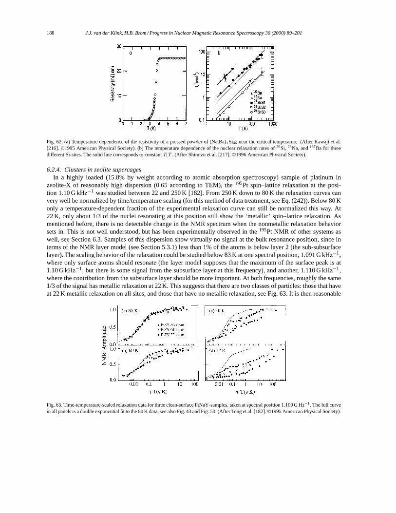
188 J.J. van der Klink, H.B. Brom / Progress in Nuclear Magnetic Resonance Spectroscopy 36 (2000) 89–201
Fig. 62. (a) Temperature dependence of the resistivity of a pressed powder of (Na,Ba)xSi46 near the critical temperature. (After Kawaji et al.[216]. ©1995 American Physical Society). (b) The temperature dependence of the nuclear relaxation rates of29Si, 23Na, and137Ba for threedifferent Si-sites. The solid line corresponds to constantT1T . (After Shimizu et al. [217]. ©1996 American Physical Society).
6.2.4. Clusters in zeolite supercagesIn a highly loaded (15.8% by weight according to atomic absorption spectroscopy) sample of platinum in
zeolite-X of reasonably high dispersion (0.65 according to TEM), the195Pt spin–lattice relaxation at the posi-tion 1.10 G kHz−1 was studied between 22 and 250 K [182]. From 250 K down to 80 K the relaxation curves canvery well be normalized by time/temperature scaling (for this method of data treatment, see Eq. (242)). Below 80 Konly a temperature-dependent fraction of the experimental relaxation curve can still be normalized this way. At22 K, only about 1/3 of the nuclei resonating at this position still show the ‘metallic’ spin–lattice relaxation. Asmentioned before, there is no detectable change in the NMR spectrum when the nonmetallic relaxation behaviorsets in. This is not well understood, but has been experimentally observed in the195Pt NMR of other systems aswell, see Section 6.3. Samples of this dispersion show virtually no signal at the bulk resonance position, since interms of the NMR layer model (see Section 5.3.1) less than 1% of the atoms is below layer 2 (the sub-subsurfacelayer). The scaling behavior of the relaxation could be studied below 83 K at one spectral position, 1.091 G kHz−1,where only surface atoms should resonate (the layer model supposes that the maximum of the surface peak is at1.10 G kHz−1, but there is some signal from the subsurface layer at this frequency), and another, 1.110 G kHz−1,where the contribution from the subsurface layer should be more important. At both frequencies, roughly the same1/3 of the signal has metallic relaxation at 22 K. This suggests that there are two classes of particles: those that haveat 22 K metallic relaxation on all sites, and those that have no metallic relaxation, see Fig. 63. It is then reasonable
Fig. 63. Time-temperature-scaled relaxation data for three clean-surface PtNaY-samples, taken at spectral position 1.100 G Hz−1. The full curvein all panels is a double exponential fit to the 80 K data, see also Fig. 43 and Fig. 50. (After Tong et al. [182]. ©1995 American Physical Society).
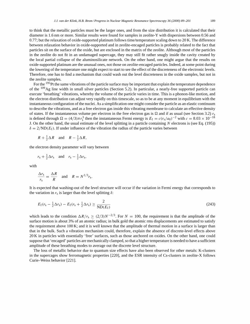
J.J. van der Klink, H.B. Brom / Progress in Nuclear Magnetic Resonance Spectroscopy 36 (2000) 89–201 189
to think that the metallic particles must be the larger ones, and from the size distribution it is calculated that theirdiameter is 1.6 nm or more. Similar results were found for samples in zeolite-Y with dispersions between 0.56 and0.77; but the relaxation of oxide-supported platinum follows time/temperature scaling down to 20 K. The differencebetween relaxation behavior in oxide-supported and in zeolite-encaged particles is probably related to the fact thatparticles sit on the surface of the oxide, but are enclosed in the matrix of the zeolite. Although most of the particlesin the zeolite do not fit in an undamaged supercage, they may still fit rather snugly inside the cavity created bythe local partial collapse of the aluminosilicate network. On the other hand, one might argue that the results onoxide-supported platinum are the unusual ones, not those on zeolite-encaged particles. Indeed, at some point duringthe lowering of the temperature one might expect to start to see the effect of the discreteness of the electronic levels.Therefore, one has to find a mechanism that could wash out the level discreteness in the oxide samples, but not inthe zeolite samples.
For the195Pt the same vibrations of the particle surface may be important that explain the temperature dependenceof the 109Ag line width in small silver particles (Section 5.2). In particular, a nearly-free supported particle canexecute ‘breathing’ vibrations, whereby the volume of the particle varies in time. This is a phonon-like motion, andthe electron distribution can adjust very rapidly on this timescale, so as to be at any moment in equilibrium with theinstantaneous configuration of the nuclei. As a simplification one might consider the particle as an elastic continuumto describe the vibrations, and as a free electron gas inside this vibrating membrane to calculate an effective densityof states. If the instantaneous volume per electron in the free electron gas is� and if as usual (see Section 3.2)rsis defined through� = (4/3)πr3
s then the instantaneous Fermi energy isEf = c(rs/a0)−2 with c = 8.03× 10⁻¹⁸
J. On the other hand, the usual estimate of the level splitting in a particle containingN electrons is (see Eq. (195))δ = 2/ND(Ef ). If under influence of the vibration the radius of the particle varies between
R + 121R and R − 1
21R,
the electron density parameter will vary between
rs+ 121rs and rs− 1
21rs,
with
1rs
rs= 1R
Rand R = N1/3rs.
It is expected that washing-out of the level structure will occur if the variation in Fermi energy that corresponds tothe variation inrs is larger than the level splittingδ:
Ef (rs− 121rs)− Ef (rs+ 1
21rs) ≥2
ND(Ef )(243)
which leads to the condition1R/rs ≥ (2/3)N−2/3. ForN = 100, the requirement is that the amplitude of thesurface motion is about 3% of an atomic radius; in bulk gold the atomic rms displacements are estimated to satisfythe requirement above 100 K; and it is well known that the amplitude of thermal motion in a surface is larger thanthat in the bulk. Such a vibration mechanism could, therefore, explain the absence of discrete-level effects above20 K in particles with essentially ‘free’ surfaces, such as those anchored on oxides. On the other hand, one couldsuppose that ‘encaged’ particles are mechanically clamped, so that a higher temperature is needed to have a sufficientamplitude of these breathing modes to average out the discrete level structure.
The loss of metallic behavior due to quantum size effects have also been observed for other metals: K-clustersin the supercages show ferromagnetic properties [220], and the ESR intensity of Cs-clusters in zeolite-X followsCurie–Weiss behavior [221].
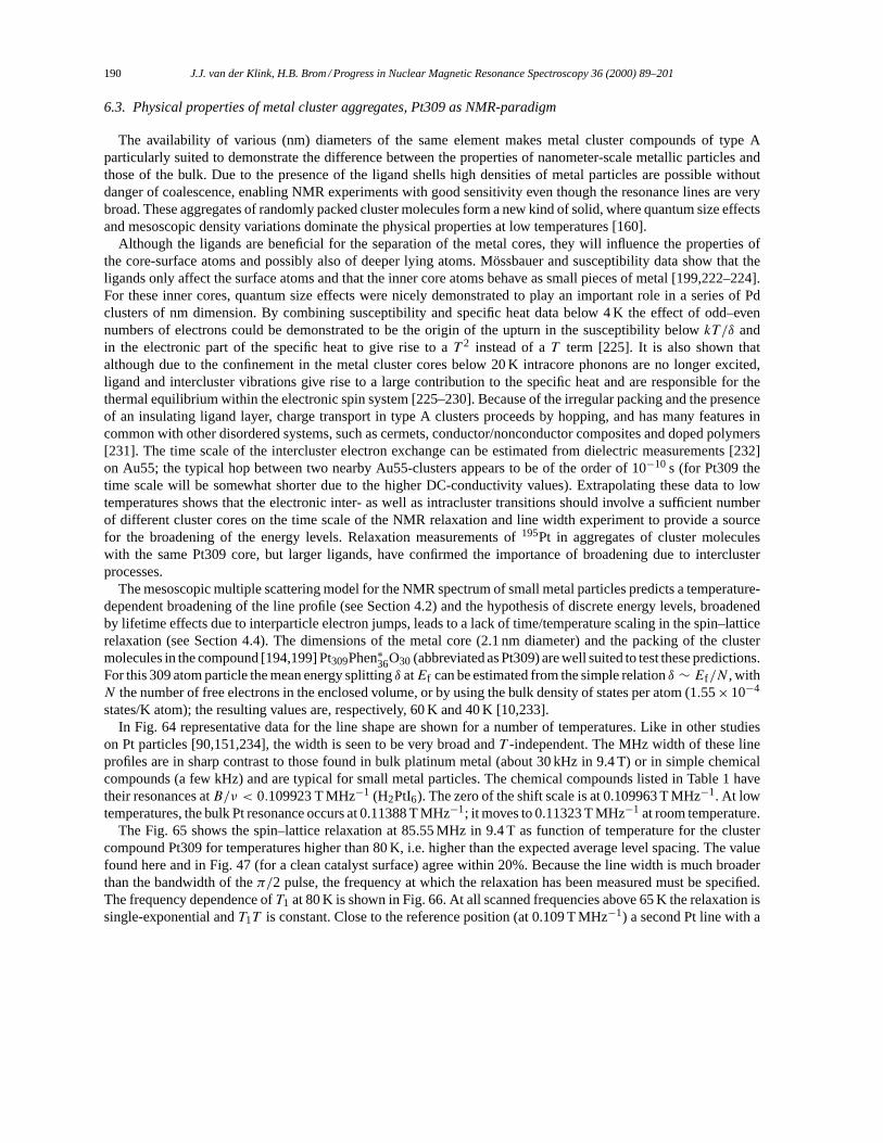
190 J.J. van der Klink, H.B. Brom / Progress in Nuclear Magnetic Resonance Spectroscopy 36 (2000) 89–201
6.3. Physical properties of metal cluster aggregates, Pt309 as NMR-paradigm
The availability of various (nm) diameters of the same element makes metal cluster compounds of type Aparticularly suited to demonstrate the difference between the properties of nanometer-scale metallic particles andthose of the bulk. Due to the presence of the ligand shells high densities of metal particles are possible withoutdanger of coalescence, enabling NMR experiments with good sensitivity even though the resonance lines are verybroad. These aggregates of randomly packed cluster molecules form a new kind of solid, where quantum size effectsand mesoscopic density variations dominate the physical properties at low temperatures [160].
Although the ligands are beneficial for the separation of the metal cores, they will influence the properties ofthe core-surface atoms and possibly also of deeper lying atoms. Mössbauer and susceptibility data show that theligands only affect the surface atoms and that the inner core atoms behave as small pieces of metal [199,222–224].For these inner cores, quantum size effects were nicely demonstrated to play an important role in a series of Pdclusters of nm dimension. By combining susceptibility and specific heat data below 4 K the effect of odd–evennumbers of electrons could be demonstrated to be the origin of the upturn in the susceptibility belowkT /δ andin the electronic part of the specific heat to give rise to aT 2 instead of aT term [225]. It is also shown thatalthough due to the confinement in the metal cluster cores below 20 K intracore phonons are no longer excited,ligand and intercluster vibrations give rise to a large contribution to the specific heat and are responsible for thethermal equilibrium within the electronic spin system [225–230]. Because of the irregular packing and the presenceof an insulating ligand layer, charge transport in type A clusters proceeds by hopping, and has many features incommon with other disordered systems, such as cermets, conductor/nonconductor composites and doped polymers[231]. The time scale of the intercluster electron exchange can be estimated from dielectric measurements [232]on Au55; the typical hop between two nearby Au55-clusters appears to be of the order of 10−10 s (for Pt309 thetime scale will be somewhat shorter due to the higher DC-conductivity values). Extrapolating these data to lowtemperatures shows that the electronic inter- as well as intracluster transitions should involve a sufficient numberof different cluster cores on the time scale of the NMR relaxation and line width experiment to provide a sourcefor the broadening of the energy levels. Relaxation measurements of195Pt in aggregates of cluster moleculeswith the same Pt309 core, but larger ligands, have confirmed the importance of broadening due to interclusterprocesses.
The mesoscopic multiple scattering model for the NMR spectrum of small metal particles predicts a temperature-dependent broadening of the line profile (see Section 4.2) and the hypothesis of discrete energy levels, broadenedby lifetime effects due to interparticle electron jumps, leads to a lack of time/temperature scaling in the spin–latticerelaxation (see Section 4.4). The dimensions of the metal core (2.1 nm diameter) and the packing of the clustermolecules in the compound [194,199] Pt309Phen∗36O30 (abbreviated as Pt309) are well suited to test these predictions.For this 309 atom particle the mean energy splittingδ atEf can be estimated from the simple relationδ ∼ Ef /N , withN the number of free electrons in the enclosed volume, or by using the bulk density of states per atom (1.55×10⁻⁴
states/K atom); the resulting values are, respectively, 60 K and 40 K [10,233].In Fig. 64 representative data for the line shape are shown for a number of temperatures. Like in other studies
on Pt particles [90,151,234], the width is seen to be very broad andT -independent. The MHz width of these lineprofiles are in sharp contrast to those found in bulk platinum metal (about 30 kHz in 9.4 T) or in simple chemicalcompounds (a few kHz) and are typical for small metal particles. The chemical compounds listed in Table 1 havetheir resonances atB/ν < 0.109923 T MHz−1 (H2PtI6). The zero of the shift scale is at 0.109963 T MHz−1. At lowtemperatures, the bulk Pt resonance occurs at 0.11388 T MHz−1; it moves to 0.11323 T MHz−1 at room temperature.
The Fig. 65 shows the spin–lattice relaxation at 85.55 MHz in 9.4 T as function of temperature for the clustercompound Pt309 for temperatures higher than 80 K, i.e. higher than the expected average level spacing. The valuefound here and in Fig. 47 (for a clean catalyst surface) agree within 20%. Because the line width is much broaderthan the bandwidth of theπ/2 pulse, the frequency at which the relaxation has been measured must be specified.The frequency dependence ofT1 at 80 K is shown in Fig. 66. At all scanned frequencies above 65 K the relaxation issingle-exponential andT1T is constant. Close to the reference position (at 0.109 T MHz−1) a second Pt line with a
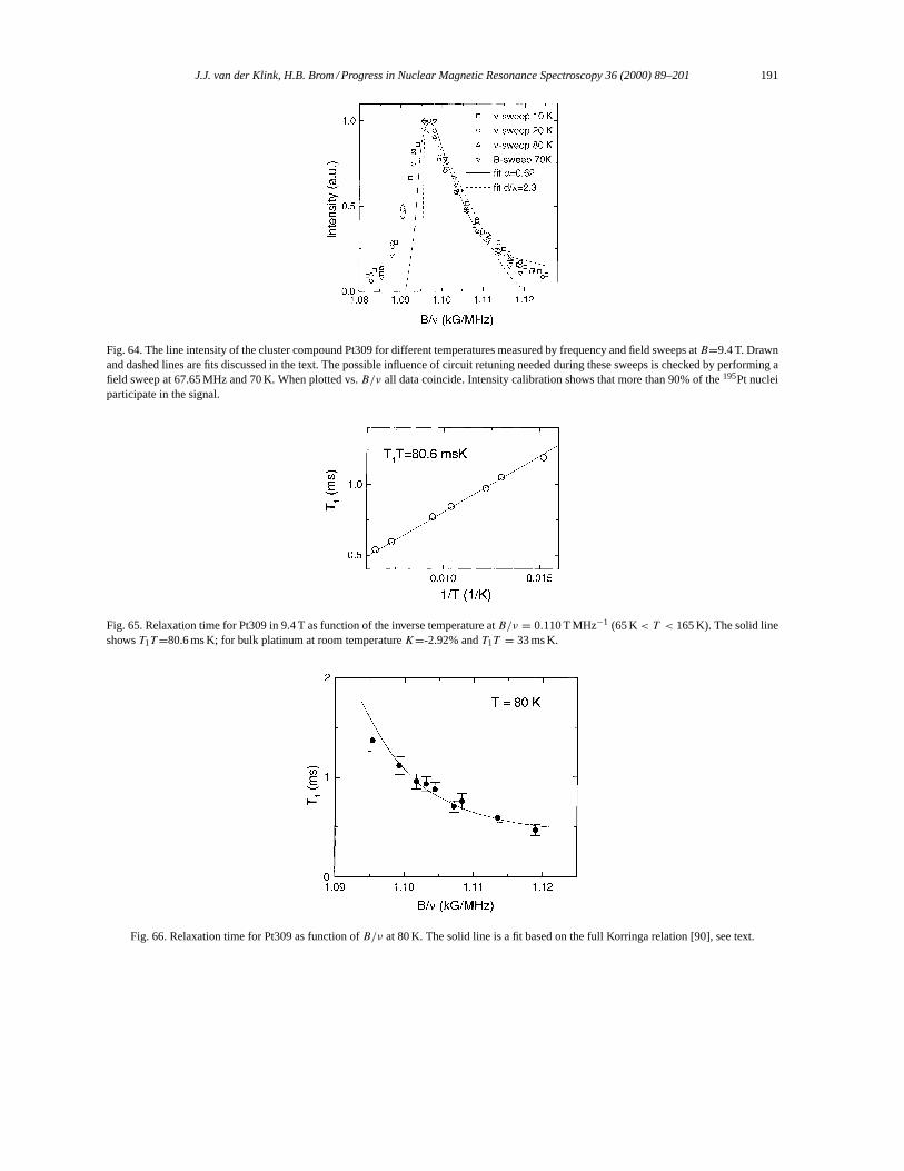
J.J. van der Klink, H.B. Brom / Progress in Nuclear Magnetic Resonance Spectroscopy 36 (2000) 89–201 191
Fig. 64. The line intensity of the cluster compound Pt309 for different temperatures measured by frequency and field sweeps atB=9.4 T. Drawnand dashed lines are fits discussed in the text. The possible influence of circuit retuning needed during these sweeps is checked by performing afield sweep at 67.65 MHz and 70 K. When plotted vs.B/ν all data coincide. Intensity calibration shows that more than 90% of the195Pt nucleiparticipate in the signal.
Fig. 65. Relaxation time for Pt309 in 9.4 T as function of the inverse temperature atB/ν = 0.110 T MHz−1 (65 K< T < 165 K). The solid lineshowsT1T=80.6 ms K; for bulk platinum at room temperatureK=-2.92% andT1T = 33 ms K.
Fig. 66. Relaxation time for Pt309 as function ofB/ν at 80 K. The solid line is a fit based on the full Korringa relation [90], see text.

192 J.J. van der Klink, H.B. Brom / Progress in Nuclear Magnetic Resonance Spectroscopy 36 (2000) 89–201
much longer relaxation time appears, which is due to Pt-atoms that are chemically strongly bound to ligand groups[233,235]. Here we neglect this second resonance.
As explained in Section 4.4, the exponential-healing models [90,151] analyze small-particle NMR data usingEq. (187)–(190), assuming that only the densities of states vary from site to site. From the combination of Knightshift and relaxation time, the s-and d-like density of states can be computed. The single exponentiality of themagnetization recoveries means that at different frequencies only one combination of s-and d-density of states isinvolved. The solid line in Fig. 66 is a fit that takes only a site dependence of the d-part of the Knight shift intoaccount [90], while the s-part is uniform. (An equally good fit can be obtained by including a healing length forthe s-electron density too [151]). The constant value ofDs(Ef ) taken in the fit is 0.28 states eV−1 at.−1, close tothe bulk value of 0.30 states eV−1 at.−1 (see Table 7). The bulk value ofDd(Ef ) (reached far from the surface) is 5times larger thanDs(Ef ).
In the calculation of the line shapeL(ν) as a function ofν the Knight shiftK has to be weighted by the numberof nuclei having that particular shift. This can be done in different ways. For the NMR layer model, similar toexponential healing, results of calculations have been illustrated in Fig. 41. The multiple scattering model givesin the case of the unitary ensemble a simple zero-Kelvin expression forL(ν), Eq. (208), which depends onlyon one parameterα, which is proportional to the ratio of the level broadeningγ and the mean level splittingδ[155,156]; for the orthogonal ensemble only small changes are expected. (Going from the unitary to the orthogonalensemble changes the second moment of the line shape at most by a factor of two [157]). With increasingT theresonance profile is predicted to shift and narrow to the bulk position and shape. Although the measured line shapecan be well fitted by the mesoscopic expression (the drawn line in Fig. 64), the expected temperature dependenceis absent. Above 65 K, where according to Fig. 65 the Korringa relation holds, the Pt309 data show that the lineshape is still broad. CalculatingL(ν)with the exponential-healing parameters that were derived from the frequencydependence of the relaxation rates in this Korringa regime,L(ν) is well reproduced [90,151,233] (dashed line inFig. 64). In this temperature range, the densities of states are smooth functions of energy, and the surface effects arebetter represented by exponential healing than by multiple scattering. Incorporating additional surface effects in themultiple scattering model by considering the different binding situation, as in Eq. (211), shows [158] that the lattereffect may indeed overshadow the other mesoscopic features. The conclusion is that at temperatures higher than65 K the spin–lattice relaxation rate and Knight shift of the Pt-cores behave as in bulk Pt, but with a reduced andsite dependent d-density of states. Up to this point, the Pt309 results are similar to those on other small Pt particlesdiscussed in Section 5.3 (but compare the discussion of platinum particles in zeolites in Section 6.2).
These common features become different below 65 K. Fig. 67 shows the recovery of the nuclear magnetizationas function of the timeτ times the temperatureT , for Pt309 at various temperatures down to 5 K. By scaling thetime as in Eq. (242), the recovery curves fall on top of each other in the Korringa regime (T > 65 K; the 80 K dataare given as reference). Non-exponentiality is observed to start below about 50 K and becomes strongly pronouncedbelow 10 K. In contrast to Korringa behavior, the scaled curves are now all temperature specific. While at 10 Kequilibrium could be reached in an hour, at 5 K it is expected that the magnetization needs at least three ordersof magnitude more for its return to the thermal equilibrium valueM0. Therefore, at 5 K,M0 is determined fromequilibrium data taken at 10 K by assuming thatM0 will obey the Curie law. For an explanation of the loss oftime-temperature scaling in Fig. 67 at 15 K and below we note that the expected average level splitting in the Pt-coreand the observed cross-over temperature are around 40 K. When thermal broadening is no longer sufficient to havea quasi-continuous density of states atEf , the differences in energy splitting become manifest, similar to what isseen in Fig. 63. The fits in Fig. 67 are based on a generalization of Eq. (227), written as
T −11 (T ,1) = A(T ) γ (T ,1)
γ 2(T ,1)+ 412, (244)
whereA(T ) is a slightly temperature-dependent proportionality constant, independent of1, andγ (T ,1) is of theform given in Eq. (228). The lines in Fig. 67 are of the form given by Eq. (235):
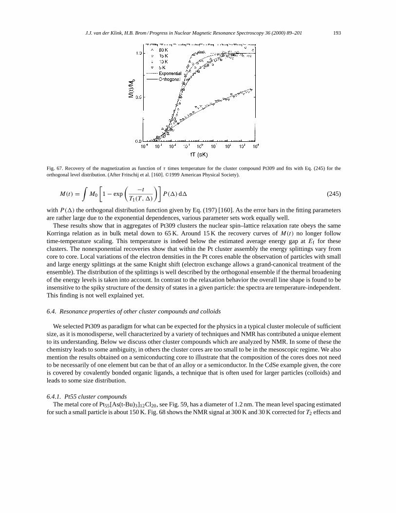
J.J. van der Klink, H.B. Brom / Progress in Nuclear Magnetic Resonance Spectroscopy 36 (2000) 89–201 193
Fig. 67. Recovery of the magnetization as function ofτ times temperature for the cluster compound Pt309 and fits with Eq. (245) for theorthogonal level distribution. (After Fritschij et al. [160]. ©1999 American Physical Society).
M(t) =∫M0
[1− exp
( −tT1(T ,1)
)]P(1)d1 (245)
with P(1) the orthogonal distribution function given by Eq. (197) [160]. As the error bars in the fitting parametersare rather large due to the exponential dependences, various parameter sets work equally well.
These results show that in aggregates of Pt309 clusters the nuclear spin–lattice relaxation rate obeys the sameKorringa relation as in bulk metal down to 65 K. Around 15 K the recovery curves ofM(t) no longer followtime-temperature scaling. This temperature is indeed below the estimated average energy gap atEf for theseclusters. The nonexponential recoveries show that within the Pt cluster assembly the energy splittings vary fromcore to core. Local variations of the electron densities in the Pt cores enable the observation of particles with smalland large energy splittings at the same Knight shift (electron exchange allows a grand-canonical treatment of theensemble). The distribution of the splittings is well described by the orthogonal ensemble if the thermal broadeningof the energy levels is taken into account. In contrast to the relaxation behavior the overall line shape is found to beinsensitive to the spiky structure of the density of states in a given particle: the spectra are temperature-independent.This finding is not well explained yet.
6.4. Resonance properties of other cluster compounds and colloids
We selected Pt309 as paradigm for what can be expected for the physics in a typical cluster molecule of sufficientsize, as it is monodisperse, well characterized by a variety of techniques and NMR has contributed a unique elementto its understanding. Below we discuss other cluster compounds which are analyzed by NMR. In some of these thechemistry leads to some ambiguity, in others the cluster cores are too small to be in the mesoscopic regime. We alsomention the results obtained on a semiconducting core to illustrate that the composition of the cores does not needto be necessarily of one element but can be that of an alloy or a semiconductor. In the CdSe example given, the coreis covered by covalently bonded organic ligands, a technique that is often used for larger particles (colloids) andleads to some size distribution.
6.4.1. Pt55 cluster compoundsThe metal core of Pt55[As(t-Bu)3]12Cl20, see Fig. 59, has a diameter of 1.2 nm. The mean level spacing estimated
for such a small particle is about 150 K. Fig. 68 shows the NMR signal at 300 K and 30 K corrected forT2 effects and
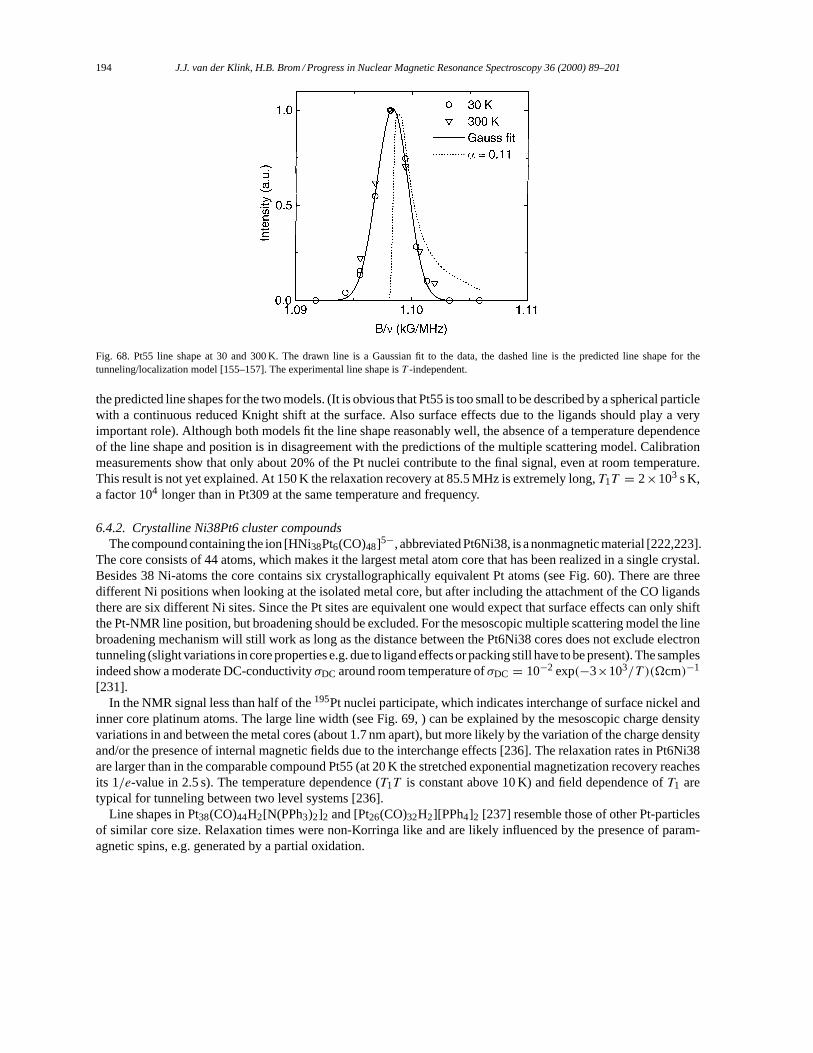
194 J.J. van der Klink, H.B. Brom / Progress in Nuclear Magnetic Resonance Spectroscopy 36 (2000) 89–201
Fig. 68. Pt55 line shape at 30 and 300 K. The drawn line is a Gaussian fit to the data, the dashed line is the predicted line shape for thetunneling/localization model [155–157]. The experimental line shape isT -independent.
the predicted line shapes for the two models. (It is obvious that Pt55 is too small to be described by a spherical particlewith a continuous reduced Knight shift at the surface. Also surface effects due to the ligands should play a veryimportant role). Although both models fit the line shape reasonably well, the absence of a temperature dependenceof the line shape and position is in disagreement with the predictions of the multiple scattering model. Calibrationmeasurements show that only about 20% of the Pt nuclei contribute to the final signal, even at room temperature.This result is not yet explained. At 150 K the relaxation recovery at 85.5 MHz is extremely long,T1T = 2×10³ s K,a factor 104 longer than in Pt309 at the same temperature and frequency.
6.4.2. Crystalline Ni38Pt6 cluster compoundsThe compound containing the ion [HNi38Pt6(CO)48]5−, abbreviated Pt6Ni38, is a nonmagnetic material [222,223].
The core consists of 44 atoms, which makes it the largest metal atom core that has been realized in a single crystal.Besides 38 Ni-atoms the core contains six crystallographically equivalent Pt atoms (see Fig. 60). There are threedifferent Ni positions when looking at the isolated metal core, but after including the attachment of the CO ligandsthere are six different Ni sites. Since the Pt sites are equivalent one would expect that surface effects can only shiftthe Pt-NMR line position, but broadening should be excluded. For the mesoscopic multiple scattering model the linebroadening mechanism will still work as long as the distance between the Pt6Ni38 cores does not exclude electrontunneling (slight variations in core properties e.g. due to ligand effects or packing still have to be present). The samplesindeed show a moderate DC-conductivityσDC around room temperature ofσDC = 10−2 exp(−3×10³/T )(�cm)−1
[231].In the NMR signal less than half of the195Pt nuclei participate, which indicates interchange of surface nickel and
inner core platinum atoms. The large line width (see Fig. 69, ) can be explained by the mesoscopic charge densityvariations in and between the metal cores (about 1.7 nm apart), but more likely by the variation of the charge densityand/or the presence of internal magnetic fields due to the interchange effects [236]. The relaxation rates in Pt6Ni38are larger than in the comparable compound Pt55 (at 20 K the stretched exponential magnetization recovery reachesits 1/e-value in 2.5 s). The temperature dependence (T1T is constant above 10 K) and field dependence ofT1 aretypical for tunneling between two level systems [236].
Line shapes in Pt38(CO)44H2[N(PPh3)2]2 and [Pt26(CO)32H2][PPh4]2 [237] resemble those of other Pt-particlesof similar core size. Relaxation times were non-Korringa like and are likely influenced by the presence of param-agnetic spins, e.g. generated by a partial oxidation.
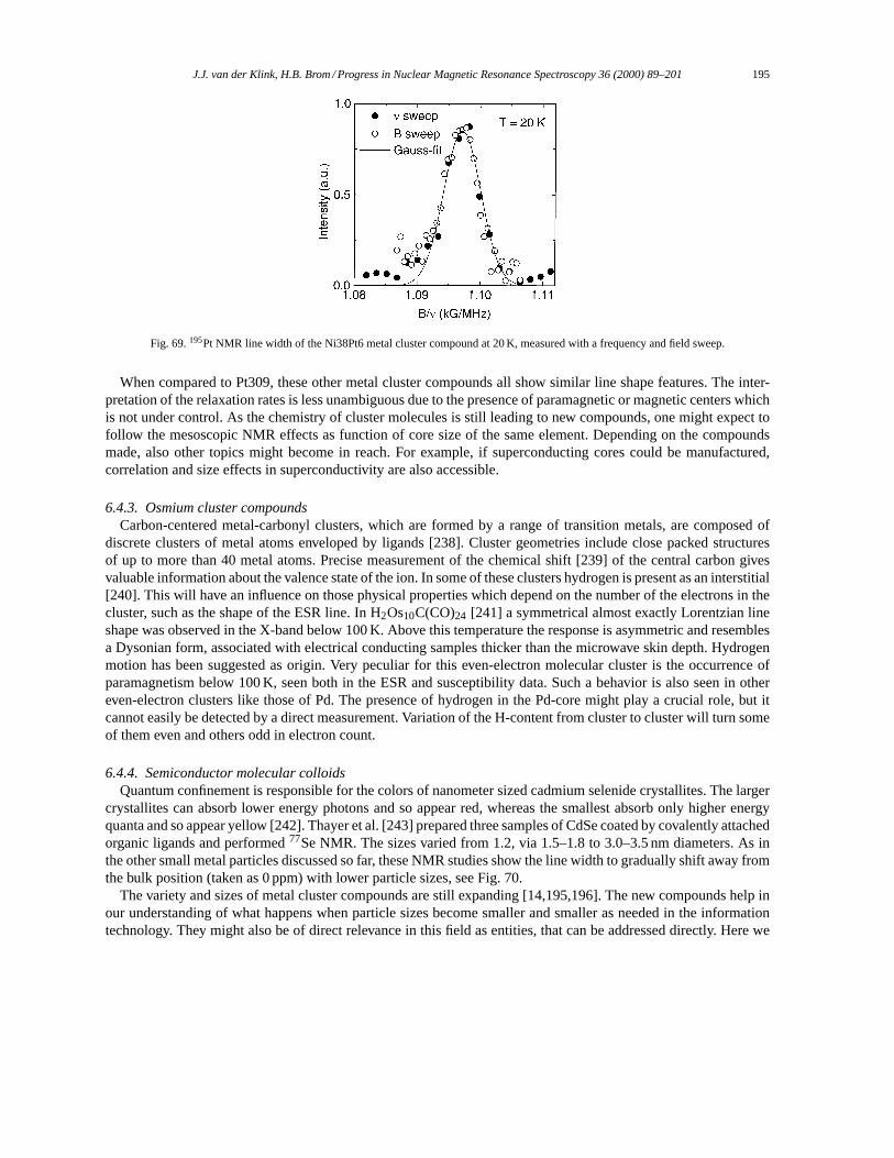
J.J. van der Klink, H.B. Brom / Progress in Nuclear Magnetic Resonance Spectroscopy 36 (2000) 89–201 195
Fig. 69.195Pt NMR line width of the Ni38Pt6 metal cluster compound at 20 K, measured with a frequency and field sweep.
When compared to Pt309, these other metal cluster compounds all show similar line shape features. The inter-pretation of the relaxation rates is less unambiguous due to the presence of paramagnetic or magnetic centers whichis not under control. As the chemistry of cluster molecules is still leading to new compounds, one might expect tofollow the mesoscopic NMR effects as function of core size of the same element. Depending on the compoundsmade, also other topics might become in reach. For example, if superconducting cores could be manufactured,correlation and size effects in superconductivity are also accessible.
6.4.3. Osmium cluster compoundsCarbon-centered metal-carbonyl clusters, which are formed by a range of transition metals, are composed of
discrete clusters of metal atoms enveloped by ligands [238]. Cluster geometries include close packed structuresof up to more than 40 metal atoms. Precise measurement of the chemical shift [239] of the central carbon givesvaluable information about the valence state of the ion. In some of these clusters hydrogen is present as an interstitial[240]. This will have an influence on those physical properties which depend on the number of the electrons in thecluster, such as the shape of the ESR line. In H2Os10C(CO)24 [241] a symmetrical almost exactly Lorentzian lineshape was observed in the X-band below 100 K. Above this temperature the response is asymmetric and resemblesa Dysonian form, associated with electrical conducting samples thicker than the microwave skin depth. Hydrogenmotion has been suggested as origin. Very peculiar for this even-electron molecular cluster is the occurrence ofparamagnetism below 100 K, seen both in the ESR and susceptibility data. Such a behavior is also seen in othereven-electron clusters like those of Pd. The presence of hydrogen in the Pd-core might play a crucial role, but itcannot easily be detected by a direct measurement. Variation of the H-content from cluster to cluster will turn someof them even and others odd in electron count.
6.4.4. Semiconductor molecular colloidsQuantum confinement is responsible for the colors of nanometer sized cadmium selenide crystallites. The larger
crystallites can absorb lower energy photons and so appear red, whereas the smallest absorb only higher energyquanta and so appear yellow [242]. Thayer et al. [243] prepared three samples of CdSe coated by covalently attachedorganic ligands and performed77Se NMR. The sizes varied from 1.2, via 1.5–1.8 to 3.0–3.5 nm diameters. As inthe other small metal particles discussed so far, these NMR studies show the line width to gradually shift away fromthe bulk position (taken as 0 ppm) with lower particle sizes, see Fig. 70.
The variety and sizes of metal cluster compounds are still expanding [14,195,196]. The new compounds help inour understanding of what happens when particle sizes become smaller and smaller as needed in the informationtechnology. They might also be of direct relevance in this field as entities, that can be addressed directly. Here we
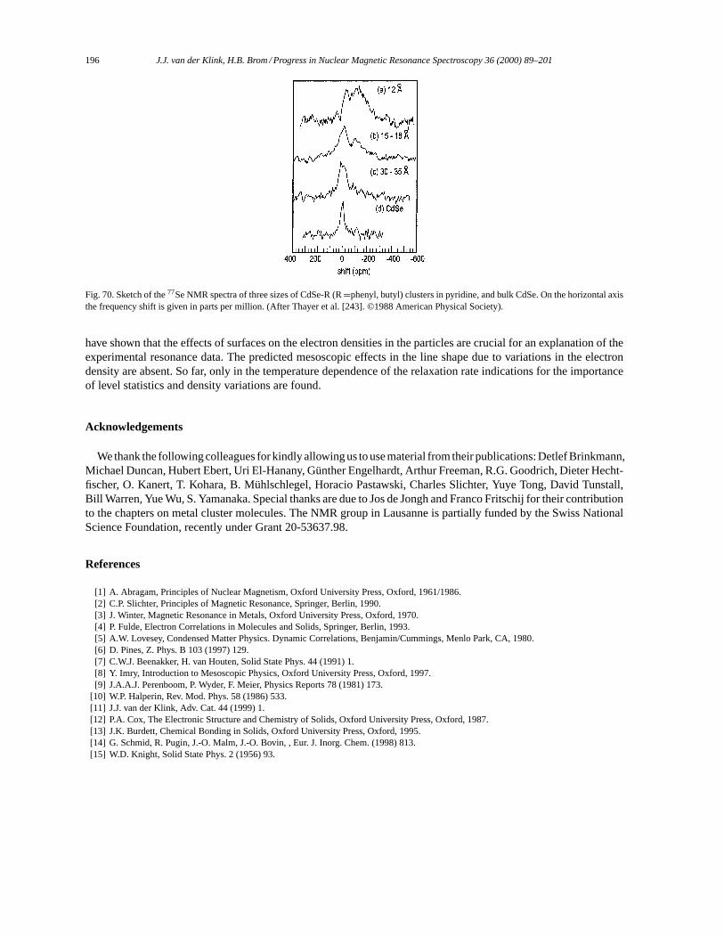
196 J.J. van der Klink, H.B. Brom / Progress in Nuclear Magnetic Resonance Spectroscopy 36 (2000) 89–201
Fig. 70. Sketch of the77Se NMR spectra of three sizes of CdSe-R (R=phenyl, butyl) clusters in pyridine, and bulk CdSe. On the horizontal axisthe frequency shift is given in parts per million. (After Thayer et al. [243]. ©1988 American Physical Society).
have shown that the effects of surfaces on the electron densities in the particles are crucial for an explanation of theexperimental resonance data. The predicted mesoscopic effects in the line shape due to variations in the electrondensity are absent. So far, only in the temperature dependence of the relaxation rate indications for the importanceof level statistics and density variations are found.
Acknowledgements
We thank the following colleagues for kindly allowing us to use material from their publications: Detlef Brinkmann,Michael Duncan, Hubert Ebert, Uri El-Hanany, Günther Engelhardt, Arthur Freeman, R.G. Goodrich, Dieter Hecht-fischer, O. Kanert, T. Kohara, B. Mühlschlegel, Horacio Pastawski, Charles Slichter, Yuye Tong, David Tunstall,Bill Warren, Yue Wu, S. Yamanaka. Special thanks are due to Jos de Jongh and Franco Fritschij for their contributionto the chapters on metal cluster molecules. The NMR group in Lausanne is partially funded by the Swiss NationalScience Foundation, recently under Grant 20-53637.98.
References
[1] A. Abragam, Principles of Nuclear Magnetism, Oxford University Press, Oxford, 1961/1986.[2] C.P. Slichter, Principles of Magnetic Resonance, Springer, Berlin, 1990.[3] J. Winter, Magnetic Resonance in Metals, Oxford University Press, Oxford, 1970.[4] P. Fulde, Electron Correlations in Molecules and Solids, Springer, Berlin, 1993.[5] A.W. Lovesey, Condensed Matter Physics. Dynamic Correlations, Benjamin/Cummings, Menlo Park, CA, 1980.[6] D. Pines, Z. Phys. B 103 (1997) 129.[7] C.W.J. Beenakker, H. van Houten, Solid State Phys. 44 (1991) 1.[8] Y. Imry, Introduction to Mesoscopic Physics, Oxford University Press, Oxford, 1997.[9] J.A.A.J. Perenboom, P. Wyder, F. Meier, Physics Reports 78 (1981) 173.
[10] W.P. Halperin, Rev. Mod. Phys. 58 (1986) 533.[11] J.J. van der Klink, Adv. Cat. 44 (1999) 1.[12] P.A. Cox, The Electronic Structure and Chemistry of Solids, Oxford University Press, Oxford, 1987.[13] J.K. Burdett, Chemical Bonding in Solids, Oxford University Press, Oxford, 1995.[14] G. Schmid, R. Pugin, J.-O. Malm, J.-O. Bovin, , Eur. J. Inorg. Chem. (1998) 813.[15] W.D. Knight, Solid State Phys. 2 (1956) 93.
J.J. van der Klink, H.B. Brom / Progress in Nuclear Magnetic Resonance Spectroscopy 36 (2000) 89–201 197
[16] T.J. Rowland, Prog. Mat. Sci. 9 (1961) 1.[17] L.E. Drain, Metallurgical Rev. 119 (1967) 195.[18] G.C. Carter, L.H. Bennett, D.J. Kahan, Prog. Mat. Sci. 20 (1977) 1.[19] R.T. Schumacher, C.P. Slichter, Phys. Rev. 101 (1956) 58.[20] R. Peierls, ZS. f. Phys. 80 (1932) 763.[21] E. Teller, ZS. f. Phys. 67 (1930) 311.[22] J. Benkowitsch, H. Winter, J. Phys. F: Met. Phys. 13 (1983) 991.[23] H. Ebert, H. Winter, J. Voitländer, J. Phys. F: Met. Phys. 16 (1986) 1133.[24] H. Ebert, M. Battocletti, M. Deng, H. Freyer, J. Voitländer, , J. Computational Chemistry, in press.[25] J.M. Luttinger, P.J. Stiles, J. Phys. Chem. Solids 17 (1961) 284.[26] D. Shoenberg, Magnetic Oscillations in Metals, Cambridge University Press, Cambridge, 1984.[27] J.A. Stratton, Electromagnetic Theory, McGraw-Hill, New York, 1941.[28] K.H. Oh, B.N. Harmon, S.H. Liu, S.K. Sinha, Phys. Rev. B 14 (1976) 1283.[29] B. Bleaney, in: A.J. Freeman, R.B. Frankel (Eds.), Hyperfine Interactions, Academic Press, New York, 1967.[30] A. Abragam, B. Bleaney, Electron Paramagnetic Resonance of Transition Ions, Oxford University Press, Oxford, 1970 (Dover reprint
1986).[31] W. Heitler, E. Teller, Proc. Roy. Soc. A 155 (1936) 629.[32] N. Bloembergen, T.J. Rowland, Phys. Rev. 97 (1955) 1679.[33] M. Ruderman, C. Kittel, Phys. Rev. 96 (1954) 99.[34] J. Korringa, Physica 16 (1950) 601.[35] H.S. Selbach, O. Kanert, D. Wolf, Phys. Rev. B 19 (1979) 4435.[36] E.C. Stoner, Proc. Roy. Soc. A 165 (1938) 372.[37] T. Moriya, J. Phys. Soc. Jpn. 18 (1963) 516.[38] Y. Yafet, V. Jaccarino, Phys. Rev. A 133 (1964) 1630.[39] S.H. Vosko, J.P. Perdew, Can. J. Phys. 53 (1975) 1385.[40] O. Gunnarson, J. Phys. F: Met. Phys. 6 (1976) 587.[41] J.F. Janak, Phys. Rev. B 16 (1977) 255.[42] A.R. Williams, U. von Barth, in: S. Lundquist, N.H. March (Eds.), Theory of the Inhomogeneous Electron Gas, Plenum Press, New York,
1983.[43] W. Götz, H. Winter, J. Phys.: Condens. Matter 4 (1992) 6253.[44] Y. Obata, J. Phys. Soc. Jpn. 18 (1963) 1020.[45] J.J. van der Klink, J. Phys.: Condens. Matter 8 (1996) 1845.[46] T. Moriya, Spin Fluctuations in Itinerant Electron Magnetism, Springer, Berlin, 1985.[47] T. Moriya, K. Ueda, Solid State Commun. 15 (1974) 169.[48] A. Ishigaki, T. Moriya, J. Phys. Soc. Jpn. 65 (1996) 3402.[49] D.E. MacLaughlin, Solid State Phys. 31 (1976) 2.[50] S.E. Barrett, D.J. Durand, C.H. Pennington, C.P. Slichter, T.A. Friedmann, Phys. Rev. B 41 (1990) 6283.[51] R.A. Ferrell, Phys. Rev. Lett. 3 (1959) 262.[52] P.W. Anderson, Phys. Rev. Lett. 3 (1959) 325.[53] J. Sone, J. Phys. Soc. Jpn. 42 (1977) 1457.[54] G. Schreckenbach, T. Ziegler, Int. J. Quantum Chem. 60 (1996) 753.[55] S. Geschwind, in: A.J. Freeman, R.B. Frankel (Eds.), Hyperfine Interactions, Academic Press, New York, 1967.[56] W.G. Proctor, F.C. Yu, Phys. Rev. 81 (1951) 20.[57] J.S. Griffith, L.E. Orgel, Trans. Faraday Soc. 53 (1957) 601.[58] R. Freeman, G.R. Murray, R.E. Richards, Proc. Roy. Soc. A 242 (1957) 455.[59] Joan Mason (Ed.), Multinuclear NMR, Plenum Press, New York, 1987.[60] A.B.P. Lever, Inorganic Electronic Spectroscopy, Elsevier, Amsterdam, 1984.[61] R. Bramley, M. Brorson, A.M. Sargeson, C.E. Schäffer, J. Am. Chem. Soc. 107 (1985) 2780.[62] M.C. Read, J. Glaser, M. Sandström, J. Chem. Soc. Dalton Trans. 233 (1992).[63] N. Juranic, J. Magn. Res. 71 (1987) 144.[64] E.R. Cohen, B.N. Taylor, Europhysics News 18 (1987) 65.[65] A. Burgstaller, J. Voitländer, H. Ebert, J. Phys.: Condens. Matter 6 (1994) 8335.[66] C. Oliver, A. Myers, J. Phys.: Condens. Matter 1 (1989) 9457.[67] Ch. Ryter, Phys. Lett. 4 (1963) 69.[68] V.L. Moruzzi, J.F. Janak, A.R. Williams, Calculated Electronic Properties of Metals, Pergamon Press, New York, 1978.[69] R.W. Shaw Jr., W.W. Warren Jr., Phys. Rev. B 3 (1971) 1562.[70] G.B. Benedek, T. Kushida, J. Phys. Chem. Solids 5 (1958) 241.[71] R. Bertani, M. Mali, J. Roos, D. Brinkmann, J. Phys.: Condens. Matter 2 (1990) 7911.
198 J.J. van der Klink, H.B. Brom / Progress in Nuclear Magnetic Resonance Spectroscopy 36 (2000) 89–201
[72] S. Kluthe, R. Markendorf, M. Mali, J. Roos, D. Brinkmann, Phys. Rev. B 53 (1996) 11369.[73] T. Kushida, J.C. Murphy, M. Hanabusa, Phys. Rev. B 13 (1976) 5136.[74] Ch. Ryter, Phys. Rev. Lett. 5 (1960) 10.[75] D.A. Papaconstantopoulos, Handbook of the Bandstructure of Elemental Solids, Plenum Press, New York, 1986.[76] B. Knecht, J. Low Temp. Phys. 21 (1975) 619.[77] W.B. Pearson, Handbook of the Lattice Spacings of Metals and Alloys, Pergamon Press, New York, 1967.[78] H.T. Weaver, A. Narath, Phys. Rev. B 1 (1970) 973.[79] U. El-Hanany, M. Shaham, D. Zamir, Phys. Rev. B 10 (1974) 2343.[80] J.-J. Bercier, Thesis EPFL, Lausanne, 1993.[81] B.S. Shastry, E. Abrahams, Phys. Rev. Lett. 72 (1994) 1933.[82] R.G. Goodrich, S.A. Khan, J.M. Reynolds, Phys. Rev. B 3 (1971) 2379.[83] A.M. Clogston, V. Jaccarino, Y. Yafet, Phys. Rev. A 134 (1964) 650.[84] M. Weinert, A.J. Freeman, Phys. Rev. B 28 (1983) 6262.[85] M. Shaham, U. El-Hanany, D. Zamir, Phys. Rev. B 17 (1978) 3513.[86] A. Narath, H.T. Weaver, Phys. Rev. 175 (1968) 373.[87] P. Bhattacharyya, K.N. Pathak, K.S. Singwi, Phys. Rev. B 3 (1971) 1568.[88] F.Y. Fradin, D.D. Koelling, A.J. Freeman, T.J. Watson-Yang, Phys. Rev. B 12 (1975) 5570.[89] L.M. Noskova, E.V. Rozenfeld, Y.P. Irkhin, Sov. Phys. Solid State 26 (1984) 1686.[90] J.P. Bucher, J.J. van der Klink, Phys. Rev. B 38 (1988) 11038.[91] A.H. MacDonald, J.M. Daams, S.H. Vosko, D.D. Koelling, Phys. Rev. B 23 (1981) 6377.[92] M.A. Fedotov, V.A. Likhobolov, Bull. Acad. Sci. USSR; Div. Chem. Sci. 33 (1984) 1751.[93] J.A. Seitchik, A.C. Gossard, V. Jaccarino, Phys. Rev. 136 (1964) A1119.[94] M. Takigawa, H. Yasuoka, J. Phys. Soc. Jpn. 51 (1982) 787.[95] N. Inoue, T. Sugawara, J. Phys. Soc. Jpn. 45 (1978) 450.[96] W. Treutmann, Z. Angew. Phys. 30 (1970) 5.[97] S. Kobayashi, H. Launois, P. Lederer, C. Froidevaux, W. Treutmann, E. Vogt, Solid State Commun. 6 (1968) 265.[98] A. Narath, H.T. Weaver, Solid State Commun. 6 (1968) 413.[99] Y.Y. Tong, T. Yonezawa, N. Toshima, J.J. van der Klink, J. Phys. Chem. 100 (1996) 730.
[100] P.A. Vuissoz, T. Yonezawa, D. Yang, J. Kiwi, J.J. van der Klink, Chem. Phys. Lett. 264 (1997) 366.[101] J.A. Seitchik, V. Jaccarino, J.H. Wernick, Phys. Rev. 138 (1965) A148.[102] A. Narath, H.T. Weaver, Phys. Rev. B 3 (1971) 616.[103] D. Hechtfischer, Z. Physik B 23 (1976) 255.[104] F. Hippert, L. Kandel, Y. Calvayrac, D. Dubost, Phys. Rev. Lett. 69 (1992) 2086.[105] Z.M. Stadnik, D. Purdie, M. Garnier, Y. Baer, A.-P. Tsai, A. Inoue, K. Edagawa, S. Takeuchi, K.H.J. Buschow, Phys. Rev. B 55 (1997)
10938.[106] G. Trambly de Laissardière, T. Fujiwara, Phys. Rev. B 50 (1994) 5999.[107] M. Krajci, M. Windisch, J. Hafner, G. Kresse, M. Mihalkovic, Phys. Rev. B 51 (1995) 17355.[108] W. Hume-Rothery, G.V. Raynor, The structure of Metals and Alloys, Institute of Metals, London, 1954.[109] A. Shastri, F. Borsa, D.R. Torgeson, J.E. Shield, A.I. Goldman, Phys. Rev. B 50 (1994) 15651.[110] A. Shastri, D.B. Baker, M.S. Conradi, F. Borsa, D.R. Torgeson, Phys. Rev. B 52 (1995) 12681.[111] J.L. Gavilano, B. Ambrosini, P. Vonlanthen, M.A. Chernikov, H.R. Ott, Phys. Rev. Lett. 79 (1997) 3058.[112] M. Mehring, H. Raber, Solid State Commun. 13 (1973) 1637.[113] E.R. Andrew, W.S. Hinshaw, R.S. Tiffen, J. Magn. Res. 15 (1974) 191.[114] Y. Obata, J. Phys. Soc. Jpn. 19 (1964) 2348.[115] X.-P. Tang, E.A. Hill, S.K. Wonnell, S.J. Poon, Y. Wu, Phys. Rev. Lett. 79 (1997) 1070.[116] W.W. Warren Jr., J. Phys.: Condens. Matter 5 (1993) B211.[117] K. Asayama, Y. Kitaoka, G.-Q. Zheng, K. Ishida, Progr. NMR Spectrosc. 28 (1996) 221.[118] C. Berthier, M.H. Julien, M. Horvatic, Y. Berthier, , J. Phys. I (France) 6 (1996) 2205.[119] H.B. Brom, Proceedings of the International School of Physics ‘Enrico Fermi’, vol. 136, 1998, p. 77.[120] W.W. Warren Jr., G.F. Brennet, U. El-Hanany, Phys. Rev. B 39 (1989) 4038.[121] A.J. Millis, H. Monien, D. Pines, Phys. Rev. B 42 (1990) 167.[122] F. Mila, T.M. Rice, Physica C 157 (1989) 561.[123] P.C. Hammel, M. Takigawa, R. Heffner, Z. Fisk, K.C. Ott, Phys. Rev. Lett. 63 (1989) 1992.[124] H. Alloul, P. Mendels, P. Monod, Phys. Rev. Lett. 61 (1988) 746.[125] H. Alloul, T. Ohno, P. Mendels, Phys. Rev. Lett. 63 (1989) 1700.[126] B. Sriram Shastry, Phys. Rev. Lett. 63 (1989) 1289.[127] W.B. Mims, G.E. Devlin, S. Geschwind, V. Jaccarino, Phys. Lett. A 24 (1967) 481.[128] W.G. Proctor, F.C. Yu, Phys. Rev. 77 (1950) 716.
J.J. van der Klink, H.B. Brom / Progress in Nuclear Magnetic Resonance Spectroscopy 36 (2000) 89–201 199
[129] P.J. Segransan, Y. Chabre, W.G. Clark, J. Phys. F 8 (1978) 1513.[130] M. Shaham, J. Barak, U. El-Hanany, W.W. Warren Jr., Phys. Rev. B 22 (1980) 5400.[131] U. El-Hanany, W.W. Warren Jr., Phys. Rev. B 12 (1975) 861.[132] Y. Kohori, Y. Noguchi, T. Kohara, J. Phys. Soc. Jpn. 62 (1993) 447.[133] M. Katayama, S. Akimoto, K. Asayama, J. Phys. Soc. Jpn. 42 (1977) 97.[134] H. Nakamura, K. Yoshimoto, M. Shiga, M. Nishi, K. Kakurai, J. Phys.: Condens. Matter 9 (1997) 4701.[135] H. Yamagata, K. Asayama, J. Phys. Soc. Jpn. 29 (1970) 1385.[136] T. Yamada, N. Kunitomi, Y. Nakai, D.E. Cox, G. Shirane, J. Phys. Soc. Jpn. 28 (1970) 615.[137] A. Narath, J. Appl. Phys. 39 (1968) 553.[138] H. Ebert, J. Abart, J. Voitländer, J. Phys. F: Met. Phys. 14 (1984) 749.[139] R. Kubo, J. Phys. Soc. Jpn. 17 (1962) 975.[140] R. Denton, B. Mühlschlegel, D.J. Scalapino, Phys. Rev. B 7 (1973) 3589.[141] E.P. Wigner, Proc. Cambridge Phil. Soc. 47 (1951) 790.[142] F.J. Dyson, J. Math. Phys. 3 (1962) 140.[143] F.J. Dyson, M.L. Mehta, J. Math. Phys. 4 (1963) 701.[144] L.P. Gorkov, G.M. Eliashberg, Sov. Phys. JETP 21 (1965) 940.[145] B.L. Altshuler, in: W.P. Kirk, M.A. Reed (Eds.), Nanostructures and Mesoscopic Systems, Elsevier, Amsterdam, 1991.[146] M.P.J. van Staveren, H.B. Brom, L.J. de Jongh, G. Schmid, Z. Phys. D 12 (1989) 451.[147] E. Cuevas, M. Ortuño, J. Ruiz, Phys. Rev. Lett. 71 (1993) 1871.[148] M.L. Mehta, Random Matrices, Academic Press, New York, 1991.[149] K.B. Efetov, Physica D 83 (1995) 151.[150] C.W.J. Beenakker, Rev. Mod. Phys. 69 (1997) 731.[151] C.D. Makowka, C.P. Slichter, J.H. Sinfelt, Phys. Rev. B 31 (1985) 5663.[152] L.I. Schiff, Quantum Mechanics, 3rd ed., McGraw-Hill, New York, 1968, pp. 83–88.[153] H.E. Rhodes, P.-K. Wang, H.T. Stokes, C.P. Slichter, J.H. Sinfelt, Phys. Rev. B 26 (1982) 3559.[154] H.T. Stokes, H.E. Rhodes, P.-K. Wang, C.P. Slichter, J.H. Sinfelt, Phys. Rev. B 26 (1982) 3575.[155] K.B. Efetov, V.N. Prigodin, Mod. Phys. Lett. B 7 (1993) 981.[156] K.B. Efetov, V.N. Prigodin, Phys. Rev. Lett. 70 (1993) 1315.[157] C. Beenakker, Phys. Rev. B 50 (1994) 15170.[158] H.M. Pastawski, J.A. Gascôn, Phys. Rev. B 56 (1997) 4887.[159] J.J. van der Klink, J. Phys.: Condens. Matter 7 (1995) 2183.[160] F.C. Fritschij, H.B. Brom, L.J. de Jongh, G. Schmid, Phys. Rev. Lett. 82 (1999) 2167.[161] L.C. Hebel, C.P. Slichter, Phys. Rev. 113 (1959) 1504.[162] S. Kobayashi, T. Takahashi, W. Sasaki, J. Phys. Soc. Jpn. 32 (1972) 1234.[163] P. Yee, W.D. Knight, Phys. Rev. B 11 (1975) 3261.[164] M.J. Williams, P.P. Edwards, D.P. Tunstall, Faraday Discuss. 92 (1991) 199.[165] D.P. Tunstall, P.P. Edwards, J. Todd, M.J. Williams, J. Phys.: Condens. Matter 6 (1994) 1791.[166] J.K. Plischke, A.J. Benesi, M.A. Vannice, J. Phys. Chem. 96 (1992) 3799.[167] V.M. Mastikhin, I.L. Mudrakovsky, S.N. Goncharova, B.S.Balzhinimaev, S.P. Noskova, V.I. Zaikovsky, React. Kinet. Catal. Lett. 48 (1992)
425.[168] J.J. Bercier, M. Jirousek, M. Graetzel, J.J. van der Klink, J. Phys.: Condens. Matter 5 (1993) L571.[169] R.J. Charles, W.A. Harrison, Phys. Rev. Lett. 11 (1963) 75.[170] J. Bardeen, Phys. Rev. 49 (1936) 653.[171] R.L. Kautz, B.B. Schwartz, Phys. Rev. B 14 (1976) 2017.[172] J.P. Bucher, J. Buttet, J.J. van der Klink, M. Graetzel, Surf. Sci. 214 (1989) 347.[173] A. Kleine, P.L. Ryder, Catal. Today 3 (1988) 103.[174] Y.Y. Tong, J.J. van der Klink, G. Clugnet, A.J. Renouprez, D. Laub, P.A. Buffat, Surf. Sci. 292 (1993) 276.[175] Y.Y. Tong, J.J. van der Klink, J. Phys. Chem. 98 (1994) 11011.[176] I. Yu, W.P. Halperin, Phys. Rev. B 47 (1993) 15830.[177] J. Ph. Ansermet, C.P. Slichter, J.H. Sinfelt, Progr. NMR Spectrosc. 22 (1990) 401.[178] S.G. Louie, Phys. Rev. Lett. 42 (1979) 476.[179] Y.Y. Tong, J.J. van der Klink, J. Phys.: Condens. Matter 7 (1995) 2447.[180] A.G. Luntz, M.D. Williams, D.S. Bethune, J. Chem. Phys. 89 (1988) 4381.[181] J.P. Bucher, J.J. van der Klink, M. Graetzel, J. Phys. Chem. 94 (1990) 1209.[182] Y.Y. Tong, D. Laub, G. Schulz-Ekloff, A.J. Renouprez, J.J. van der Klink, Phys. Rev. B 52 (1995) 8407.[183] Y.Y. Tong, J.J. Billy, A.J. Renouprez, J.J. van der Klink, J. Am. Chem. Soc. 119 (1997) 3929.[184] Y.Y. Tong, P. Meriaudeau, A.J. Renouprez, J.J. van der Klink, J. Phys. Chem. B 101 (1997) 10155.[185] Y.Y. Tong, C. Belrose, A. Wieckowski, E. Oldfield, J. Am. Chem. Soc. 119 (1997) 11709.
200 J.J. van der Klink, H.B. Brom / Progress in Nuclear Magnetic Resonance Spectroscopy 36 (2000) 89–201
[186] C. Rice, Y.Y. Tong, E. Oldfield, A. Wieckowski, Electrochim. Acta 43 (1998) 2825.[187] S. Ladas, R.A. Dalla Betta, M. Boudart, J. Catal. 53 (1978) 356.[188] D.A. van Leeuwen, J.M. van Ruitenbeek, G. Schmid, L.J. de Jongh, Phys. Lett. A 170 (1992) 325.[189] N. Toshima, T. Yonezawa, K. Kushihashi, J. Chem. Soc. Faraday Trans. 89 (1993) 2537.[190] A. Eichler, J. Hafner, J. Furthmüller, G. Kresse, Surf. Sci. 346 (1996) 300.[191] R. Löber, D. Hennig, Phys. Rev. B 55 (1997) 4761.[192] A. Ceriotti, F. Demartin, G. Longoni, M. Manassero, G. Piva, M. Sansoni, Angew. Chem. Ed. Engl. 24 (1985) 697.[193] H. Krautscheid, D. Fenske, G. Baum, M. Semmelmann, Angew. Chem. 105 (1993) 1364.[194] G. Schmid, Clusters and colloids: from theory to applications, in: G. Schmid (Ed.), Structure and Bonding, vol. 62, VCH, Weinheim,
1985, p. 51.[195] R.L. Whetten, J.T. Khoury, M.M. Alvarez, S. Murthy, I. Veznar, Z.L. Wang, P.W. Stephens, C.L. Cleveland, W.D. Luedtke, U. Landman,
Adv. Mater. 8 (1996) 428.[196] A. Müller, S.Q.N. Shah, H. Bögge, M. Schmidtmann, Nature 397 (1999) 48.[197] H. Nakayama, D.D. Klug, C.I. Ratcliffe, J.A. Ripmeester, J. Am. Chem. Soc. 116 (1994) 9777.[198] L.J. Woodall, P.A. Anderson, A.R. Armstrong, P.P. Edwards, J. Chem. Soc. Dalton Trans. (1996) 719.[199] L.J. de Jongh (Ed.), Physics and Chemistry of Metal Cluster Compounds, Kluwer Academic Publishers, Dordrecht, 1994.[200] A. Ceriotti, R. Pergola, L. Garlaschelli, Physics and Chemistry of Metal Cluster Compounds, Kluwer Academic Publishers, Dordrecht,
1994.[201] A. Ecker, E. Weckert, H. Schnöckel, Nature 387 (1997) 397.[202] A. Lasciafari, Z.H. Jang, F. Borsa, P. Caretta, D. Gatteschi, Phys. Rev. Lett. 81 (1998) 3773.[203] J. Klinowski, Progr. NMR Spectrosc. 16 (1984) 237.[204] J.B. Nagy, I. Hannus, I. Kiricsi, in: J.H. Fendler (Ed.), Nanoparticles and Nanostructured Films, Wiley-VCH, Weinheim, 1998.[205] O.F. Sankey, A.A. Demkov, T. Lenovsky, Phys. Rev. B 57 (1998) 15129.[206] P.J. Grobet, G. van Gorp, L.R.M. Martens, P.A. Jacobs, Proc. Coll. Ampere 23 (1986) 356.[207] P.A. Anderson, P.P. Edwards, J. Am. Chem. Soc. 114 (1992) 10608.[208] E. Trescos, F. Rachdi, L.C. de Ménorval, F. Fajula, T. Numes, G. Feio, J. Phys. Chem. 97 (1993) 11855.[209] N.P. Blake, V.I. Srdanov, G.D. Stucky, H. Metiu, J. Chem. Phys. 104 (1996) 8721.[210] G. Engelhardt, M. Feuerstein, P. Sieger, D. Markgraber, G. Stucky, V. Srdanov, J. Chem. Soc. Chem. Commun. (1996) 729.[211] V.I. Srdanov, G.D. Stucky, E. Lippmaa, G. Engelhardt, Phys. Rev. Lett. 80 (1998) 2449.[212] C. Cros, M. Pouchard, P. Hagemuller, Compt. Rend. 260 (1965) 4764.[213] J.S. Kasper, P. Hagemuller, M. Pouchard, C. Cros, Science 150 (1965) 1714.[214] A.A. Demkov, O.F. Sankey, K.E. Schmidt, G.B. Adams, M.O’Keeffe, Phys. Rev. B 50 (1994) 17001.[215] S.B. Roy, K.E. Sim, A.D. Caplin, Phil. Mag. B 6 (1992) 1445.[216] H. Kawaji, H. Horie, S. Yamanaka, M. Ishikawa, Phys. Rev. Lett. 74 (1995) 1427.[217] F. Shimizu, Y. Maniwa, K. Kume, H. Kawaji, S. Yamanaka, M. Ishikawa, Phys. Rev. B 54 (1996) 13242.[218] J. Gryko, P.F. MacMillan, R.F. Marzke, A.P. Dodokin, A.A. Demkov, O.F. Sankey, Phys. Rev. B 57 (1998) 4172.[219] G.B. Adams, M. O’Keeffe, A.A. Demkov, O.F. Sankey, Y-M. Huang, Phys. Rev. B 49 (1994) 8048.[220] Y. Nozue, T. Kodaira, S. Ohwashi, T. Goto, O. Terasaki, Phys. Rev. B. 48 (1993) 12253.[221] K.W. Blazey, K.A. Müller, F. Blatter, E. Schumacher, Europhys. Lett. 4 (1987) 857.[222] D. van Leeuwen, J. van Ruitenbeek, Phys. Rev. Lett. 73 (1994) 1423.[223] David A. van Leeuwen, J.M. van Ruitenbeek, L.J. de Jongh, A. Ceriotti, G. Pacchioni, O.D. Häberlen, N. Rösch, Phys. Rev. Lett. 73
(1994) 1432.[224] F.M. Mulder, T.A. Stegink, R.C. Thiel, L.J. de Jongh, G. Schmid, Nature 367 (1994) 716.[225] Y. Volokitin, J. Sinzig, L.J. de Jongh, G. Schmid, M.N. Vargaftik, I.I. Moiseev, Nature 384 (1996) 621.[226] H.H.A. Smit, P.R. Nugteren, R.C. Thiel, L.J. de Jongh, Physica B 153 (1988) 33.[227] J. Baak, H.B. Brom, L.J. de Jongh, G. Schmid, Z. Phys. D 26 (1993) S30.[228] H.B. Brom, J. Baak, in: L.J. de Jongh (Ed.), Physics and Chemistry of Metal Cluster Compounds, Kluwer Academic Publishers, Dordrecht,
1994, p. 211.[229] Y. Volokitin, J. Sinzig, G. Schmid, H. Bonnemann, L.J. de Jongh, Z. Phys. D 40 (1997) 136.[230] Y. Volokitin, C. Bernard, G. Schmid, I.I. Moiseev, L.J. de Jongh, Czech. J. Phys 46 (Suppl. S4) 2373 (1996).[231] M.P.J. van Staveren, H.B. Brom, L.J. de Jongh, Phys. Rep. 208 (1991) 1.[232] J.A. Reedijk, H.B. Brom, L.J. de Jongh, G. Schmid, Phys. Rev. B 57 (1998) R15116.[233] H.B. Brom, D. van der Putten, L.J. de Jongh, Physics and Chemistry of Metal Cluster Compounds, Kluwer Academic Publishers, Dordrecht,
1994, p. 227.[234] I. Yu, W.P. Halperin, J. Low Temp. Phys. 45 (1981) 189.[235] D. van der Putten, H.B. Brom, L.J. de Jongh, G. Schmid, in: P. Jena (Ed.), Physics and Chemistry of Finite Systems: From Clusters to
Crystals, Kluwer Academic Publishers, Dordrecht, 1992, p. 1007.[236] H.B. Brom, J.J. van der Klink, F.C. Fritschij, L.J. de Jongh, R. della Pergola, A. Ceriotti, Z. Phys. D 40 (1997) 559.
J.J. van der Klink, H.B. Brom / Progress in Nuclear Magnetic Resonance Spectroscopy 36 (2000) 89–201 201
[237] B.J. Pronk, H.B. Brom, A. Ceriotti, G. Longoni, Solid State. Commun. 64 (1987) 7.[238] P. Chini, J. Organomet. Chem. 200 (1980) 37.[239] J.D. Harris, T. Hughbanks, J. Am. Chem. Soc. 119 (1997) 9449.[240] E.C. Constable, B.F.G. Johnson, J. Lewis, G.N. Pain, M.J. Taylor, J. Chem. Soc. Chem. Commun. (1982) 754.[241] R.E. Benfield, J. Phys. Chem. 91 (1987) 2712.[242] M.A. Reed, Scientific American, January 1993, 98.[243] A.M. Thayer, M.L. Steigerwald, T.M. Duncan, D.C. Douglas, Phys. Rev. Lett. 60 (1988) 2673.