Embed Size (px)
Citation preview

7/25/2019 NM Lecture 6 on 15th Sept 2015.pdf
http://slidepdf.com/reader/full/nm-lecture-6-on-15th-sept-2015pdf 1/76
NUMERICAL METHODS
Lecture 6
Dr. P V Ramana 1NM Dr P V RAMANA
7/25/2019 NM Lecture 6 on 15th Sept 2015.pdf
http://slidepdf.com/reader/full/nm-lecture-6-on-15th-sept-2015pdf 2/76
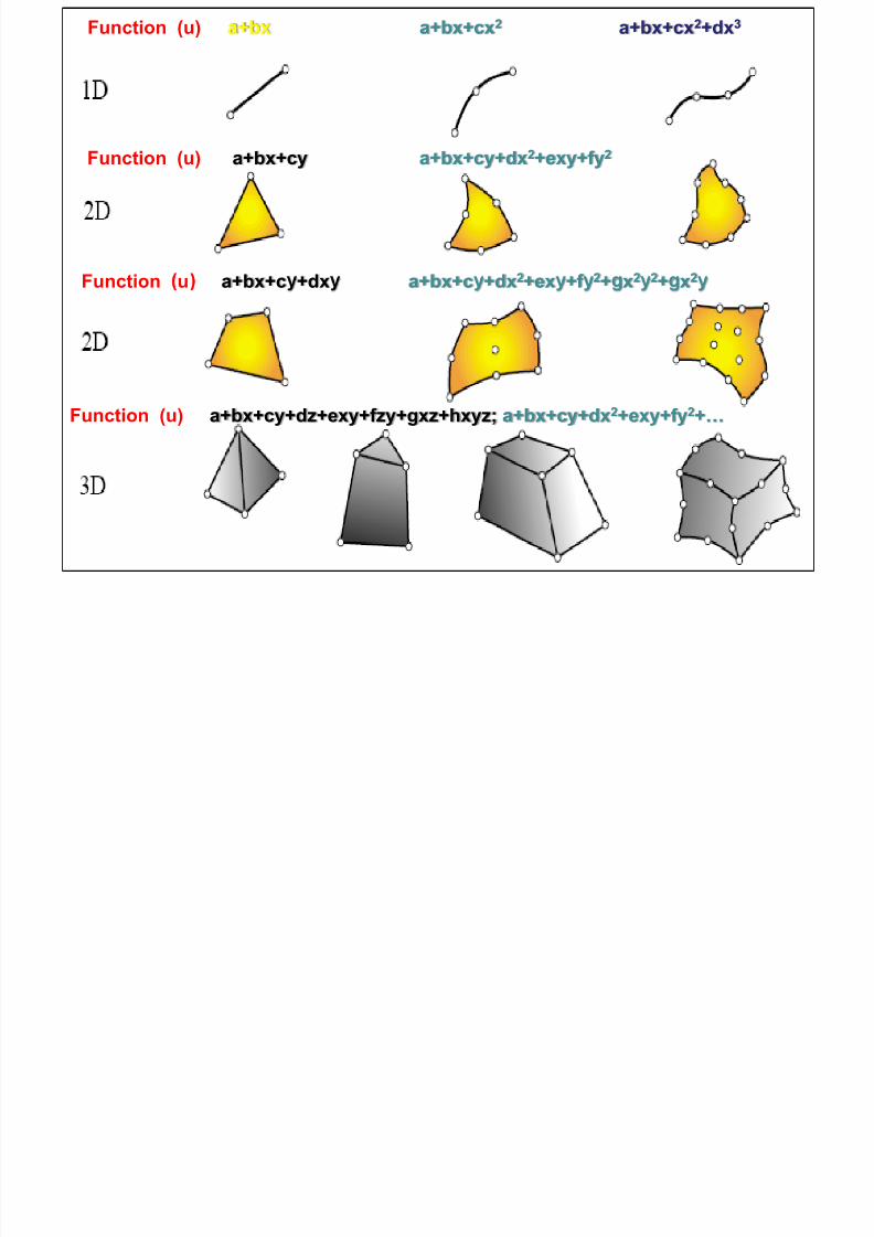
Function (u) a+bx a+bx+cx2 a+bx+cx2+dx3
Function (u) a+bx+cy a+bx+cy+dx2+exy+fy2
Function u a+bx+c +dx a+bx+c +dx2+ex +f 2+ x2 2+ x2
Function (u) a+bx+cy+dz+exy+fzy+gxz+hxyz; a+bx+cy+dx2+exy+fy2+…
NM Dr P V RAMANA 2

7/25/2019 NM Lecture 6 on 15th Sept 2015.pdf
http://slidepdf.com/reader/full/nm-lecture-6-on-15th-sept-2015pdf 3/76
Forces are acting in transverse
direction
3NM Dr P V
RAMANA
7/25/2019 NM Lecture 6 on 15th Sept 2015.pdf
http://slidepdf.com/reader/full/nm-lecture-6-on-15th-sept-2015pdf 4/76
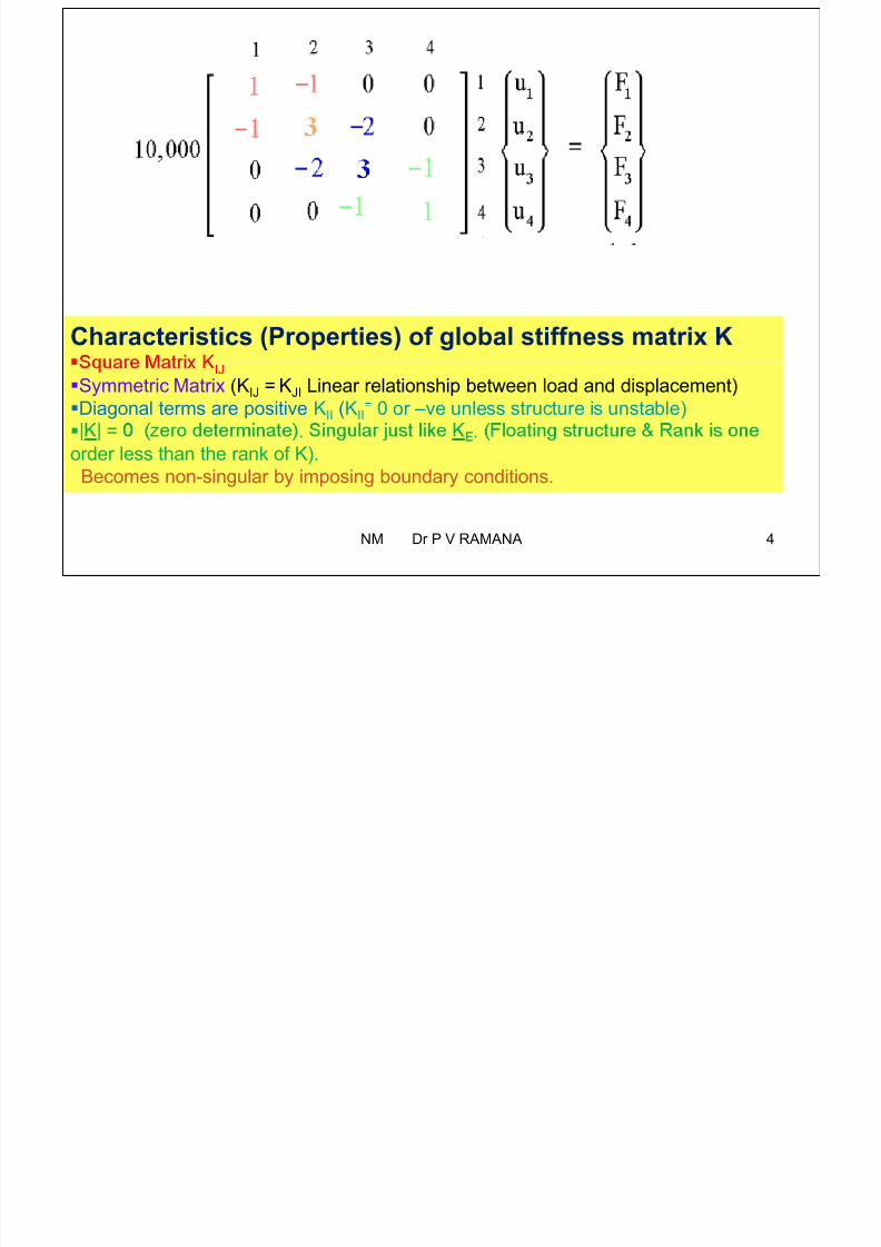
Characteristics (Properties) of global stiffness matrix K IJ
Symmetric Matrix (KIJ = KJI Linear relationship between load and displacement)
Diagonal terms are positive KII (KII= 0 or –ve unless structure is unstable) = . .
order less than the rank of K).
Becomes non-singular by imposing boundary conditions.
NM Dr P V RAMANA 4
7/25/2019 NM Lecture 6 on 15th Sept 2015.pdf
http://slidepdf.com/reader/full/nm-lecture-6-on-15th-sept-2015pdf 5/76
•
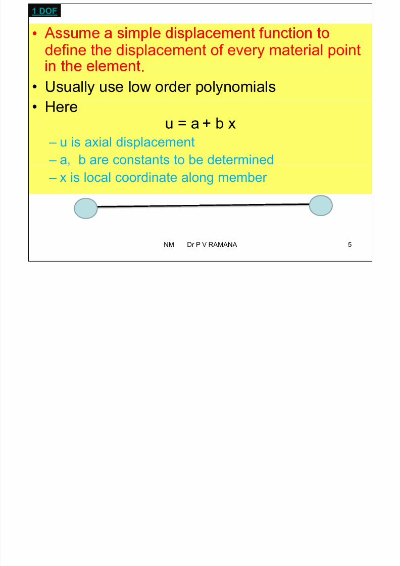
1 DOF
define the displacement of every material point.
• Usually use low order polynomials• Here
u = a + b x
– u is axial displacement – a b are constants to be determined
– x is local coordinate along member
NM Dr P V RAMANA 5
7/25/2019 NM Lecture 6 on 15th Sept 2015.pdf
http://slidepdf.com/reader/full/nm-lecture-6-on-15th-sept-2015pdf 6/76
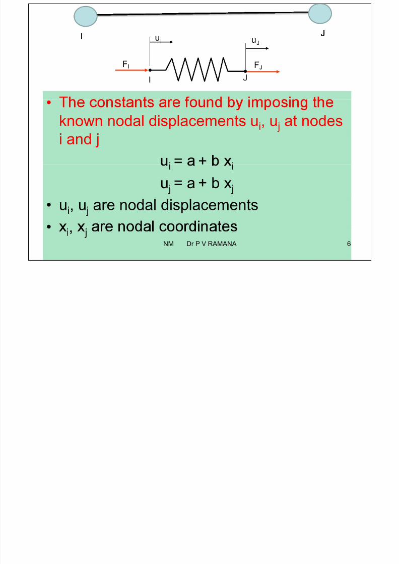
uJ
F F
uI
I J
•
known nodal displacements ui, u j at nodes
i and j= +
u j = a + b x j
• ui, u j are nodal displacements
• i, j 6NM Dr P V RAMANA
7/25/2019 NM Lecture 6 on 15th Sept 2015.pdf
http://slidepdf.com/reader/full/nm-lecture-6-on-15th-sept-2015pdf 7/76
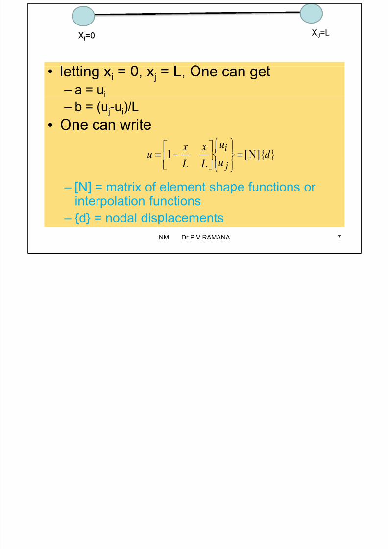
=I
• e ng xi = , x j = , ne can ge
– a = ui
– b = (u j-ui)/L
•
}]{ N[1 d u x x
u i
– N = matrix of element sha e functions or
u j
interpolation functions
– d = nodal dis lacements
7NM Dr P V RAMANA
7/25/2019 NM Lecture 6 on 15th Sept 2015.pdf
http://slidepdf.com/reader/full/nm-lecture-6-on-15th-sept-2015pdf 8/76
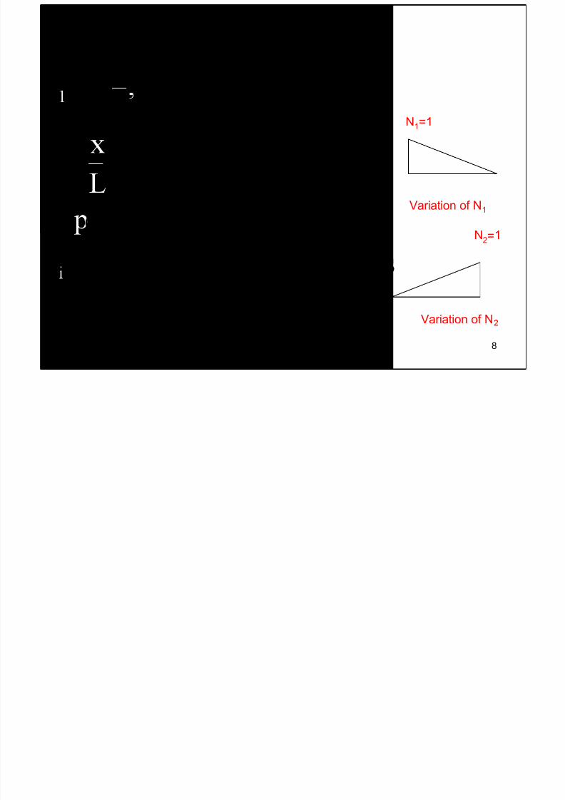
1 2 N N N
xN 1 L
N1=1
2N
Pro ertiesVariation of N1
N 1 at node i and zero at all other nodes
2=
i N 1 Variation of N
1 2i.e. at any point in the element N N 1 8NM Dr P V RAMANA
7/25/2019 NM Lecture 6 on 15th Sept 2015.pdf
http://slidepdf.com/reader/full/nm-lecture-6-on-15th-sept-2015pdf 9/76
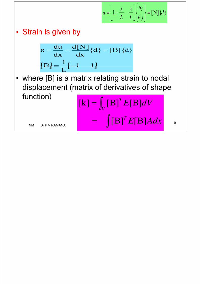
}]{ N[1 d u x x
u i
•
du d[N]dx dx
1
• where [B] is a matrix relating strain to nodalL
displacement (matrix of derivatives of shape
functiondV E
V ]B[]B[]k [
NM Dr P V RAMANA9 Adx E T ]B[]B[
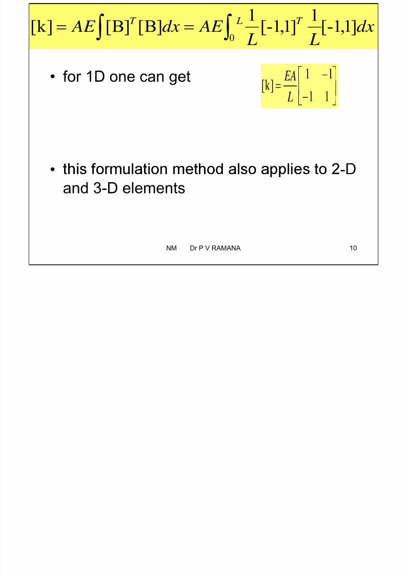
7/25/2019 NM Lecture 6 on 15th Sept 2015.pdf
http://slidepdf.com/reader/full/nm-lecture-6-on-15th-sept-2015pdf 10/76
dx AE dx AE T LT
]1,1-[1
]1,1-[1
]B[]B[]k [
• for 1D one can get
11]k[
L
EA
• -
and 3-D elements
10NM Dr P V RAMANA
P bl 1

7/25/2019 NM Lecture 6 on 15th Sept 2015.pdf
http://slidepdf.com/reader/full/nm-lecture-6-on-15th-sept-2015pdf 11/76
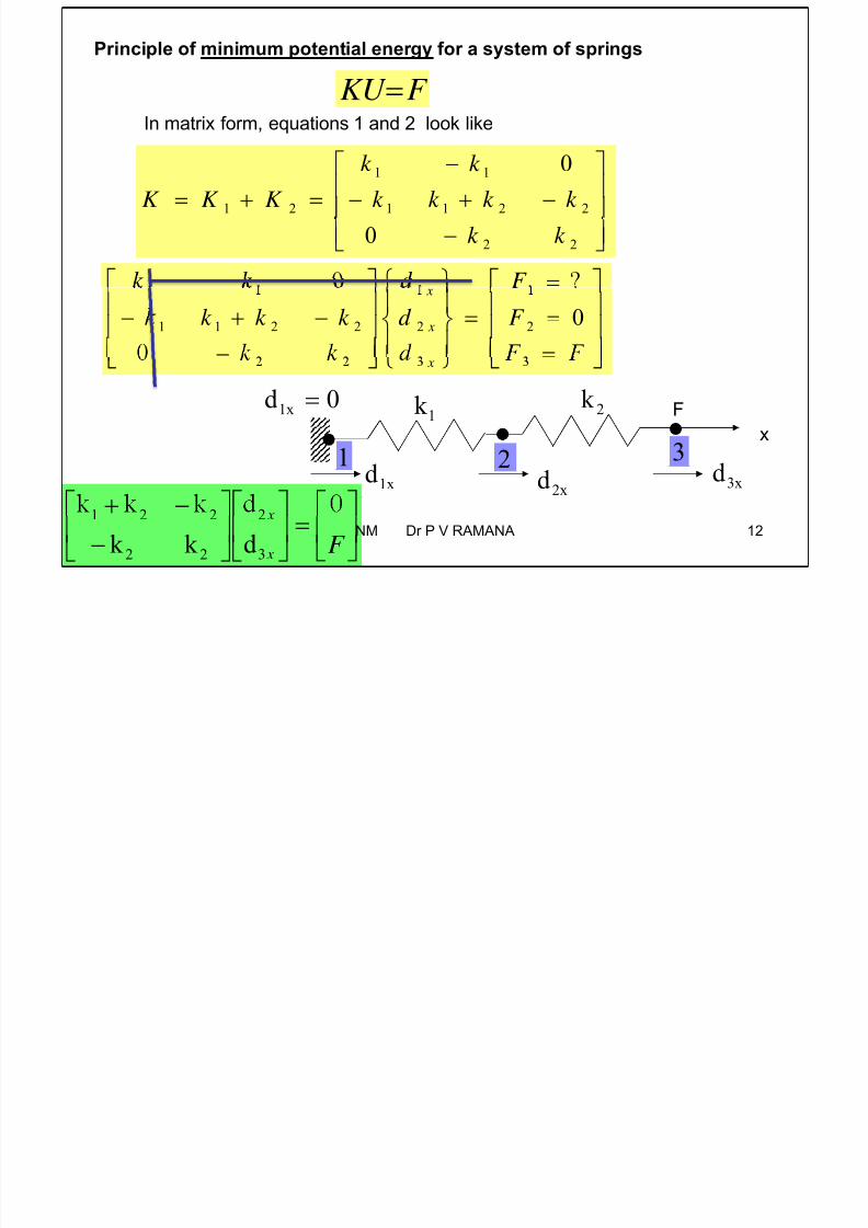
For a system of springs
Problem 1
1k Fx
2k 0d1x
1xd2xd 3xd
,
as:
2211 k k k k
222
111 k k k k
11 0k k
221121 k k k k K K K
11
NM Dr P V RAMANA 22
7/25/2019 NM Lecture 6 on 15th Sept 2015.pdf
http://slidepdf.com/reader/full/nm-lecture-6-on-15th-sept-2015pdf 12/76
32

7/25/2019 NM Lecture 6 on 15th Sept 2015.pdf
http://slidepdf.com/reader/full/nm-lecture-6-on-15th-sept-2015pdf 13/76
3
3
2
210)( xa xa xaa xv 2 DOF
321 32)( xa xaa xv
NM Dr P V RAMANA 13
7/25/2019 NM Lecture 6 on 15th Sept 2015.pdf
http://slidepdf.com/reader/full/nm-lecture-6-on-15th-sept-2015pdf 14/76

7/25/2019 NM Lecture 6 on 15th Sept 2015.pdf
http://slidepdf.com/reader/full/nm-lecture-6-on-15th-sept-2015pdf 15/76
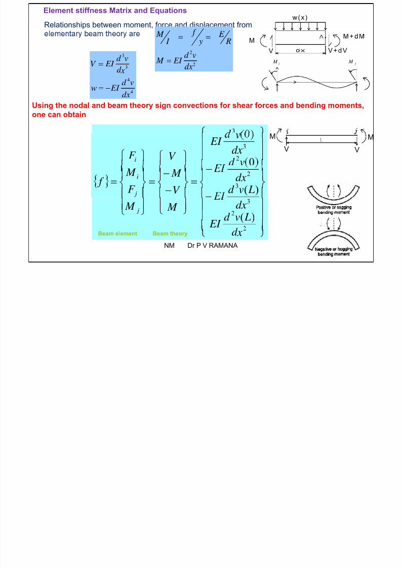
Use the following equations into above equation.
3 (0)d v
M M
V V
22323
3231
11
2,32 xL L x L x L
N L L x x L
N
3
2
2
(0)i
i
dx
F V d v EI
M M dx
3433 ,
L L 3
2
2
( )
j
j
v EI
M dx M
d v L
EI dx
d N v
d dxdx
vd d dxdx
vd d dxdx
dv ,,33
3
22
2
EI N d 22
2
Ldx,,,
3
NM Dr P V RAMANA 15 L L Ldx
6,12,6,1233
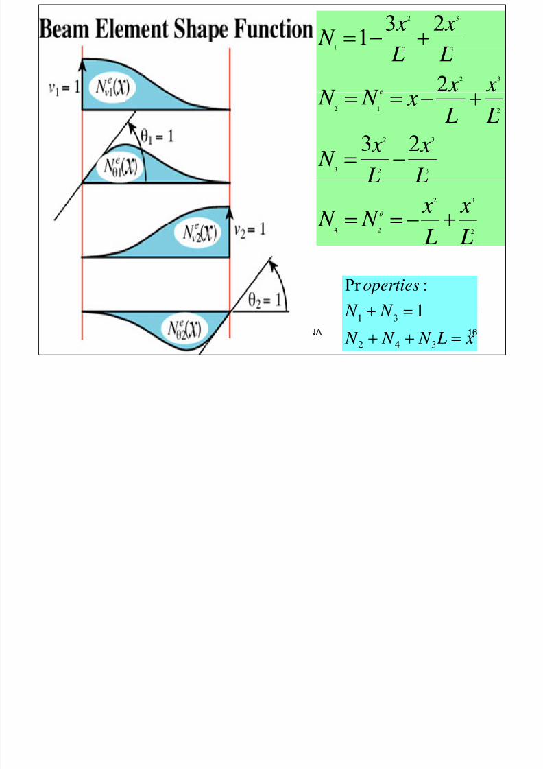
7/25/2019 NM Lecture 6 on 15th Sept 2015.pdf
http://slidepdf.com/reader/full/nm-lecture-6-on-15th-sept-2015pdf 16/76
32 231
x x N
322 x x212
L L x
3
3
2
2
3
x x N
32
x x
224
L L
operties :Pr
x L N N N 342
31NM Dr P V RAMANA 16
7/25/2019 NM Lecture 6 on 15th Sept 2015.pdf
http://slidepdf.com/reader/full/nm-lecture-6-on-15th-sept-2015pdf 17/76
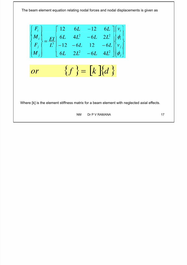
The beam element equation relating nodal forces and nodal displacements is given as
ii v L LF 612612
ii
v L L
L L L L
L
EI
F
M 22
3 612612
2646
j j L L L L M 22 4626
d k f or
Where [k] is the element stiffness matrix for a beam element with neglected axial effects.
NM Dr P V RAMANA 17

7/25/2019 NM Lecture 6 on 15th Sept 2015.pdf
http://slidepdf.com/reader/full/nm-lecture-6-on-15th-sept-2015pdf 18/76

7/25/2019 NM Lecture 6 on 15th Sept 2015.pdf
http://slidepdf.com/reader/full/nm-lecture-6-on-15th-sept-2015pdf 19/76
NM Dr P V RAMANA 19
AE AE
3 DOF
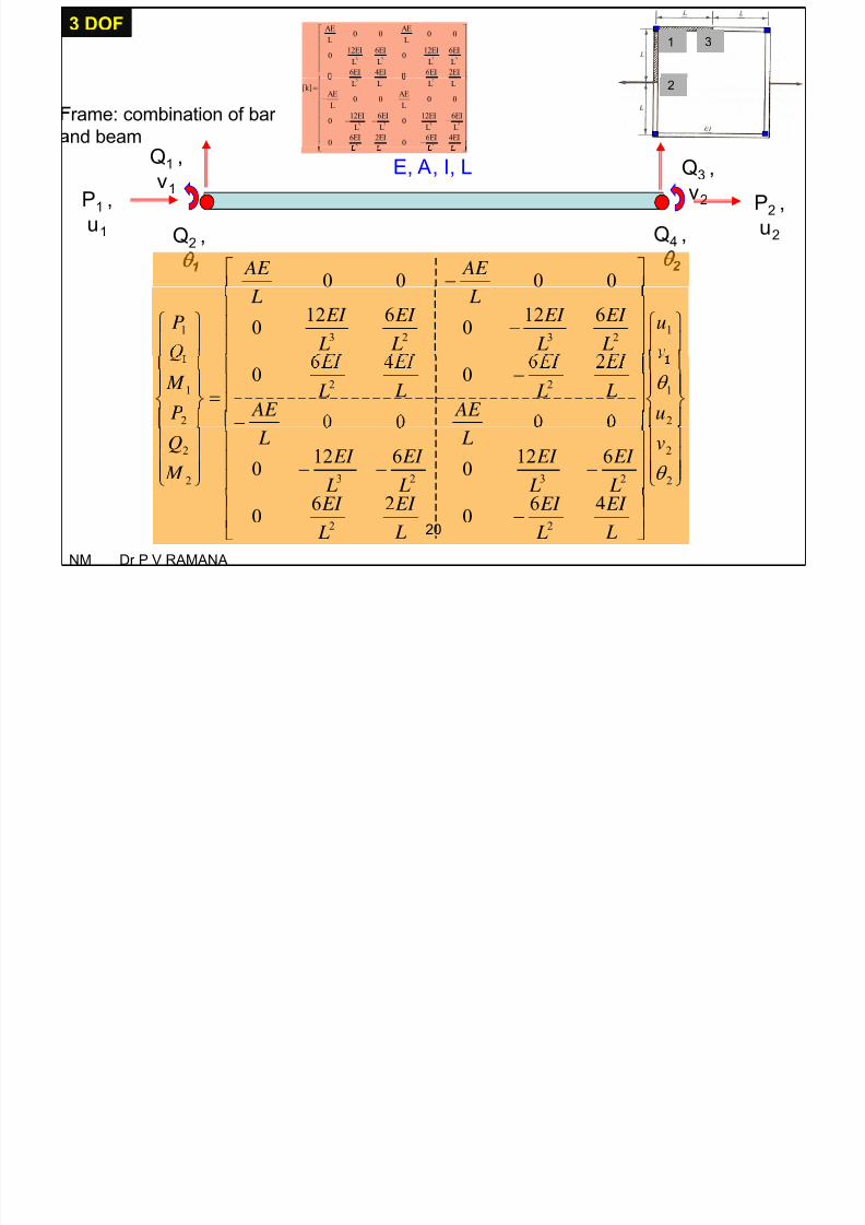
7/25/2019 NM Lecture 6 on 15th Sept 2015.pdf
http://slidepdf.com/reader/full/nm-lecture-6-on-15th-sept-2015pdf 20/76
3 2 3 2
AE AE0 0 0 0
L L
12EI 6EI 12EI 6EI0 0
L L L L
6EI 4EI 6EI 2EI
1 3
3 DOF
rame: combination of bar
nd beam
2 2
3 2 3 2
2 2
L L L L[k]
AE AE0 0 0 0
L L12EI 6EI 12EI 6EI
0 0L L L L
6EI 2EI 6EI 4EI0 0
2
E, A, I, LQ1 ,
v1
Q3 ,
v2P1 , P2 ,
Q2 ,
1
u1 Q4 ,
2
u2
0000
AE AE
1
23231
6120
6120 u
L
EI
L
EI
L
EI
L
EI L L
P
2
122
2
100
u AE AE
L L L L
P
M
2
2
23232
2 6120
6120
v
L
EI
L
EI
L
EI
L
EI L L
M
Q
22460260 L EI
L EI
L EI
L EI
20
NM Dr P V RAMANA

7/25/2019 NM Lecture 6 on 15th Sept 2015.pdf
http://slidepdf.com/reader/full/nm-lecture-6-on-15th-sept-2015pdf 21/76
GJ GJ
L L
3 2 3 20 0
L L L L
3 30 0
L L L L
GJ GJ0 0 0 0
12EI 6EI 12EI 6EI0 0
6EI 2EI 6EI 4EI
2 2L L L L 21
NM Dr P V RAMANA
F d t l C t
7/25/2019 NM Lecture 6 on 15th Sept 2015.pdf
http://slidepdf.com/reader/full/nm-lecture-6-on-15th-sept-2015pdf 22/76
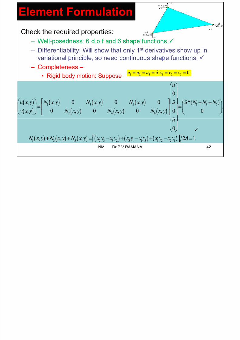
Fundamental Concepts
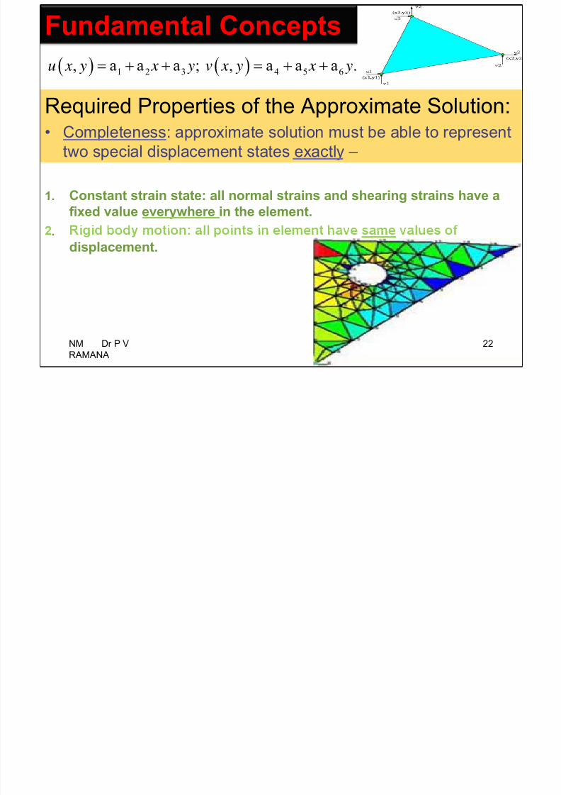
1 2 3 4 5 6, a a a ; , a a a .u x y x y v x y x y
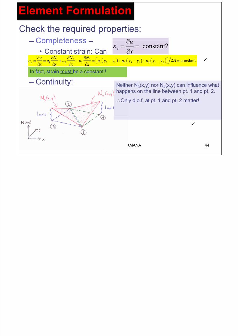
Required Properties of the Approximate Solution:
• Completeness: approximate solution must be able to representtwo special displacement states exactly –
1. Constant strain state: all normal strains and shearing strains have afixed value everywhere in the element.
.
displacement.
NM Dr P V
RAMANA
22
F d t l C t
7/25/2019 NM Lecture 6 on 15th Sept 2015.pdf
http://slidepdf.com/reader/full/nm-lecture-6-on-15th-sept-2015pdf 23/76
Fundamental Concepts
Required Properties of the Approximate Solution:• e -pose ness: e num er o s ape unc ons use
in the approximate solution must equal the number of degrees
.
Degrees of freedom are the unknowns in the local problem;
.
E.g., Galerkin and Rayleigh’s method
NM Dr P V RAMANA 23
El t F l ti
7/25/2019 NM Lecture 6 on 15th Sept 2015.pdf
http://slidepdf.com/reader/full/nm-lecture-6-on-15th-sept-2015pdf 24/76
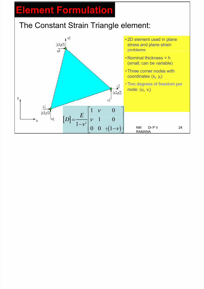
Element Formulation
The Constant Strain Triangle element:
• 2D element used in plane
stress and plane strain
roblems
• Nominal thickness = h
(small; can be variable)
• Three corner nodes withcoordinates (xi, yi)
node: (ui, vi)
1 0
NM Dr P V
RAMANA
24 2
12
1 010 0 1
D
Element Formulation
7/25/2019 NM Lecture 6 on 15th Sept 2015.pdf
http://slidepdf.com/reader/full/nm-lecture-6-on-15th-sept-2015pdf 25/76
Element Formulation
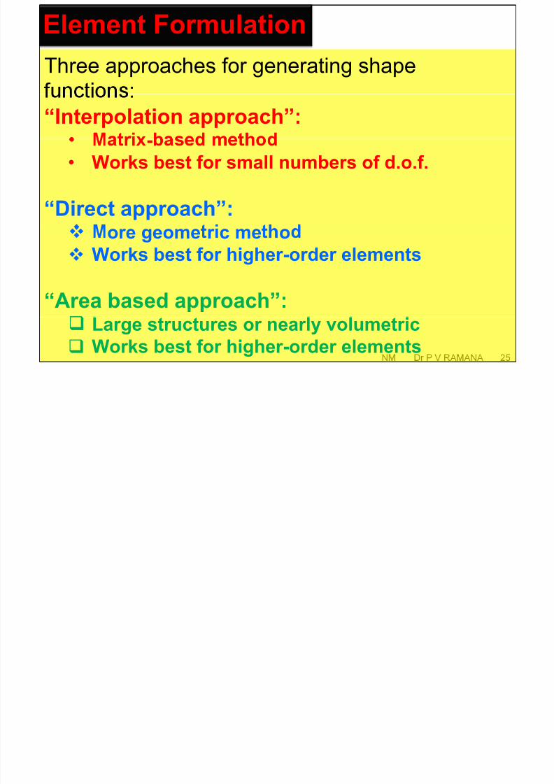
Three approaches for generating shape
“Interpolation approach”:-
• Works best for small numbers of d.o.f.
“Direct approach”:ore geome r c me o
Works best for higher-order elements
“Area based approach”:
NM Dr P V RAMANA 25
Large structures or nearly volumetric Works best for higher-order elements
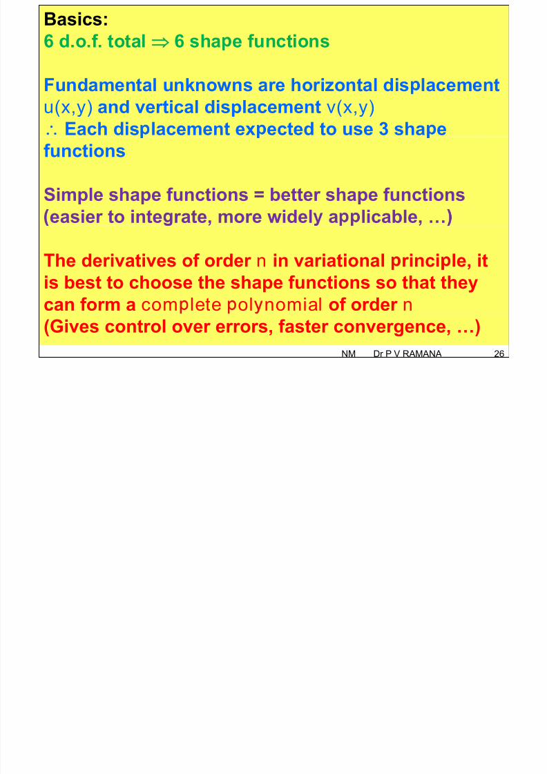
Basics:
7/25/2019 NM Lecture 6 on 15th Sept 2015.pdf
http://slidepdf.com/reader/full/nm-lecture-6-on-15th-sept-2015pdf 26/76
Basics:
6 d.o.f. total 6 sha e functions
Fundamental unknowns are horizontal dis lacement
u(x,y) and vertical displacement v(x,y)
Each dis lacement ex ected to use 3 sha efunctions
Simple shape functions = better shape functionseasier to inte rate, more widel a licable, …
The derivatives of order n in variational rinci le, itis best to choose the shape functions so that they
can form a com lete ol nomial of order n
NM Dr P V RAMANA 26
(Gives control over errors, faster convergence, …)
Element Formulation

7/25/2019 NM Lecture 6 on 15th Sept 2015.pdf
http://slidepdf.com/reader/full/nm-lecture-6-on-15th-sept-2015pdf 27/76
Element Formulation
“Interpolation approach”:st , ,
1 2 3 4 5 6, a a a ; , a a a .u x y x y v x y x y
– At each node, require u(xi,yi) = ui and v(xi,yi) = vi :
1 1 2 1 3 1 1 4 5 1 6 1
2 1 2 2 3 2 2 4 5 2 6 2
.
a a a ; a a a .u x y v x y
3 1 2 3 3 3 3 4 5 3 6 3.
6 e uations for the 6 unknowns!
NM Dr P V
RAMANA
27
1 1 2 1 3 1 1 4 5 1 6 1a a a ; a a a .u x y v x y
Element Formulation
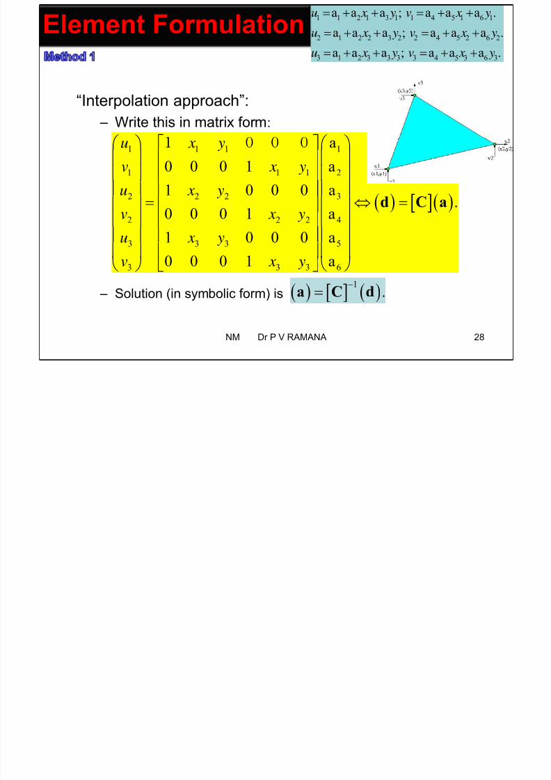
7/25/2019 NM Lecture 6 on 15th Sept 2015.pdf
http://slidepdf.com/reader/full/nm-lecture-6-on-15th-sept-2015pdf 28/76
2 1 2 2 3 2 2 4 5 2 6 2a a a ; a a a .u x y v x y Element Formulation3 1 2 3 3 3 3 4 5 3 6 3a a a ; a a a .u x y v x y
“Interpolation approach”:
– Write this in matrix form:
1 1 1 1
1 1 1 2
a
0 0 0 1 a
u x y
v x y
2 2 2 3
2 2 2 4
1 0 0 0 a .0 0 0 1 a
u x yv x y
d C a
3 3 3 5
3 3 3 6
1 0 0 0 a
0 0 0 1 a
u x y
v x y
– Solution (in symbolic form) is 1
.
a C d
NM Dr P V RAMANA 28
Element Formulation
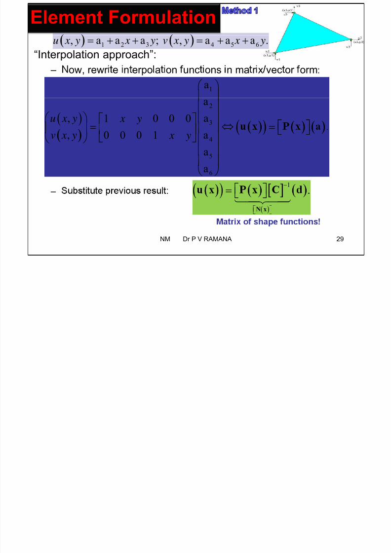
7/25/2019 NM Lecture 6 on 15th Sept 2015.pdf
http://slidepdf.com/reader/full/nm-lecture-6-on-15th-sept-2015pdf 29/76
Element Formulation
“Interpolation approach”:1 2 3 4 5 6, a a a ; , a a a .u x y x y v x y x y
– ow, rewr e n erpo a on unc ons n ma r x vec or orm:
1a
2
3
a
, a1 0 0 0u x y x y
4
5
, a0 0 0 1a
v x y x y
–
6a
1
.
N x
NM Dr P V RAMANA 29
Element Formulation
7/25/2019 NM Lecture 6 on 15th Sept 2015.pdf
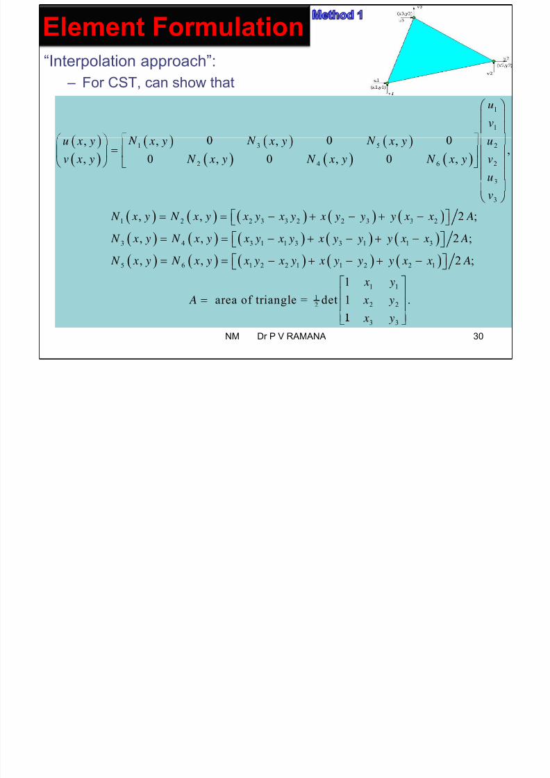
http://slidepdf.com/reader/full/nm-lecture-6-on-15th-sept-2015pdf 30/76
Element Formulation
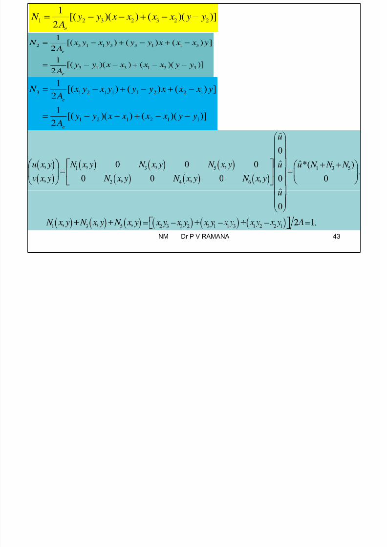
“Interpolation approach”: – For CST, can show that
1
1
u
v
21 3 5
22 4 6
, , , ,,
, 0 , 0 , 0 ,
uu x y x y x y x y
vv x y N x y N x y N x y
u
3
1 2 2 3 3 2 2 3 3 2 , , 2 ;
v
N x y N x y x y x y x y y y x x A
3 4 3 1 1 3 3 1 1 3 , , N x y N x y x y x y x y y y x x
5 6 1 2 2 1 1 2 2 1
2 ;
, , 2 ;
A
N x y N x y x y x y x y y y x x A
1 1
12 22
1
area of triangle = det 1 .
x y
A x y
3 3
x y
NM Dr P V RAMANA 30
Element Formulation

7/25/2019 NM Lecture 6 on 15th Sept 2015.pdf
http://slidepdf.com/reader/full/nm-lecture-6-on-15th-sept-2015pdf 31/76
Element Formulation
Notes on “Interpolation approach”:
– s approac genera zes o eren s apes, eren no e
locations, and different numbers of d.o.f.
– However, the matrix [C] is not always invertible for general
choices of nodal locations.
– As number of d.o.f. increases, matrix inversion becomes more
difficult, and thus exact functions become harder to determine.
NM Dr P V
RAMANA
31
Element Formulation
7/25/2019 NM Lecture 6 on 15th Sept 2015.pdf
http://slidepdf.com/reader/full/nm-lecture-6-on-15th-sept-2015pdf 32/76
Element Formulation
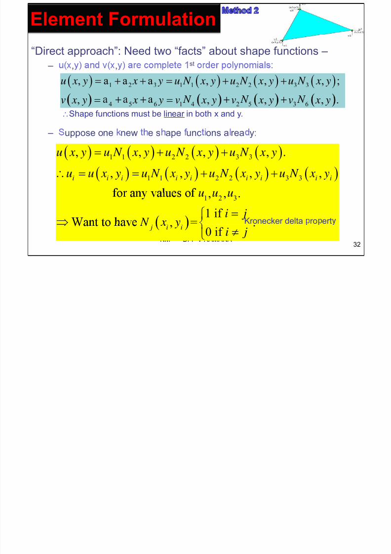
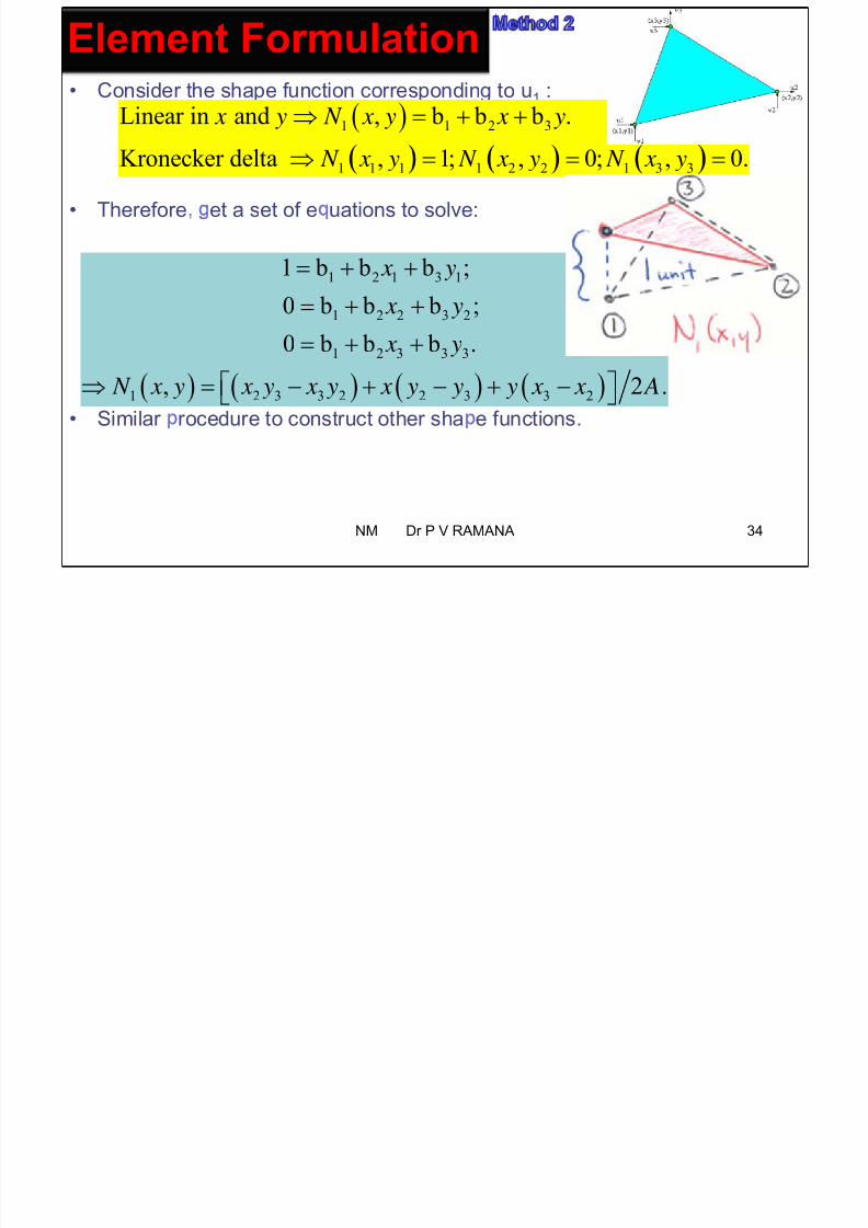
“Direct approach”: Need two “facts” about shape functions – – st, ,
1 2 3 1 1 2 2 3 3, a a a , , , ;u x y x y u N x y u N x y u N x y
4 5 6 1 4 2 5 3 6, , , , .v x y x y v x y v x y v x y Shape functions must be linear in both x and y.
– uppose one new e s ape unc ons a rea y:
1 1 2 2 3 3, , , , .u x y u N x y u N x y u N x y
1 1 2 2 3 3, , , ,i i i i i i i i iu u x y u N x y u N x y u N x y
1 2 3 , , .
1 if=
i jKronecker delta ro ert
NM Dr P V RAMANA32
, .0 if
j i i
i j
Element Formulation

7/25/2019 NM Lecture 6 on 15th Sept 2015.pdf
http://slidepdf.com/reader/full/nm-lecture-6-on-15th-sept-2015pdf 33/76
Element Formulation
• Visually, this looks like:
NM Dr P V RAMANA 33
7/25/2019 NM Lecture 6 on 15th Sept 2015.pdf
http://slidepdf.com/reader/full/nm-lecture-6-on-15th-sept-2015pdf 34/76
Shape functions construction

7/25/2019 NM Lecture 6 on 15th Sept 2015.pdf
http://slidepdf.com/reader/full/nm-lecture-6-on-15th-sept-2015pdf 35/76
Shape functions construction
1 1
2 2 2 3 3 2 2 3 1 3 2 1
11 1 1
1 [( ) ( ) ( ) ]
2 2 2e
x y
x y x y x y y y x x x y P
3 3 x y
Area of triangle Moment matrix
Substitute a1, b1 and c1 back into N1 = a1 + b1x + c1y:
1 2 3 2 3 2 2
1[( )( ) ( )( )]
2 e
N y y x x x x y y
A
35NM Dr P V RAMANA
Shape functions construction
7/25/2019 NM Lecture 6 on 15th Sept 2015.pdf
http://slidepdf.com/reader/full/nm-lecture-6-on-15th-sept-2015pdf 36/76
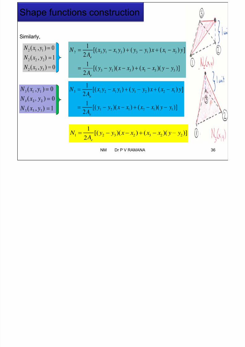
Shape functions construction
Similarly,
2 1 1
2 2 2
( , ) 0
( , ) 1
N x y
N x y
2 3 1 1 3 3 1 1 3
1[( ) ( ) ( ) ]
2 e
N x y x y y y x x x y A
2 3 3( , ) 0 N x y 3 1 3 1 3 3
1[( )( ) ( )( )]
2 e
y y x x x x y y A
3 1 1( , ) 0
0
N x y
N x
3 1 2 1 1 1 2 2 11 [( ) ( ) ( ) ]2 e
N x y x y y y x x x y A
3 3 3( , ) 1 N x y 1 2 1 2 1 1
1[( )( ) ( )( )]
2 e
y y x x x x y y A
1 2 3 2 3 2 2
1[( )( ) ( )( )]
2 N y y x x x x y y
NM Dr P V RAMANA 36
Shape functions construction
7/25/2019 NM Lecture 6 on 15th Sept 2015.pdf
http://slidepdf.com/reader/full/nm-lecture-6-on-15th-sept-2015pdf 37/76
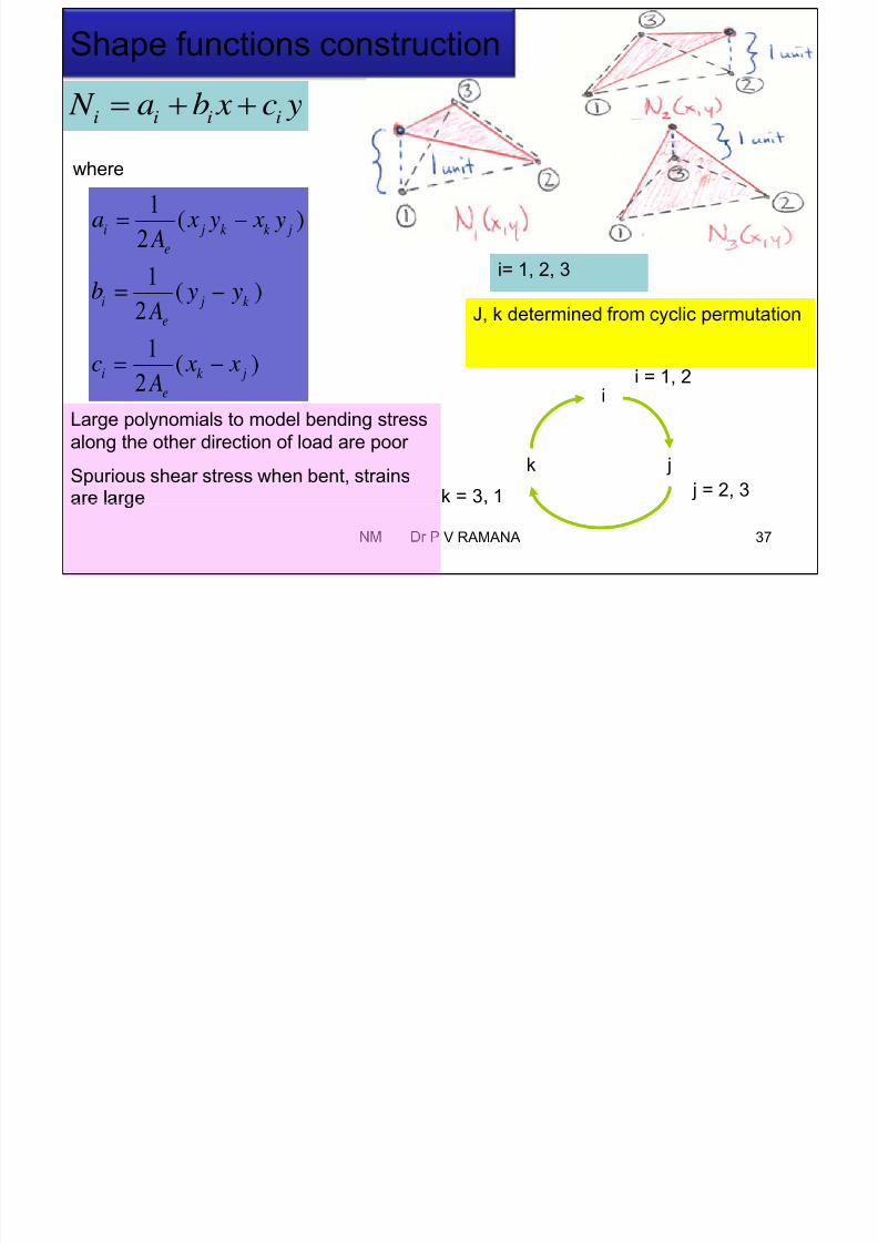
Shape functions construction
i i i i N a b x c y
1
where
2
1
i j k k j
e A
i= 1, 2, 3
21
i j k
e A
J, k determined from cyclic permutation
2i k j
e A
ii = 1, 2
Large polynomials to model bending stress
jk
j = 2, 3k = 3 1
along the other direction of load are poor
Spurious shear stress when bent, strains
NM Dr P V RAMANA 37
Using area coordinates
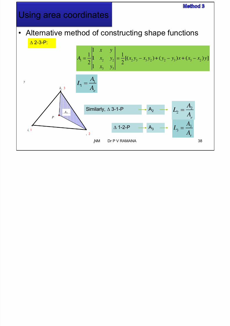
7/25/2019 NM Lecture 6 on 15th Sept 2015.pdf
http://slidepdf.com/reader/full/nm-lecture-6-on-15th-sept-2015pdf 38/76
Using area coordinates
• Alternative method of constructing shape functions
1
1 1
x y
2-3-P:
1 2 2 2 3 3 2 2 3 3 2
3 3
2 21 x y
k , 3 y 11
e
A L
A1 Similarly, 3-1-P A2 22
A L
i, 1
P
1-2-P A3
e
33
A L
38
, 2
xe
NM Dr P V RAMANA
Using area coordinates1
1 1 x y
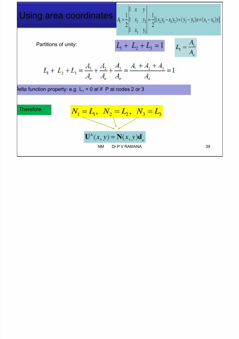
7/25/2019 NM Lecture 6 on 15th Sept 2015.pdf
http://slidepdf.com/reader/full/nm-lecture-6-on-15th-sept-2015pdf 39/76
Using area coordinates 1 11 A x x x x x x
3 3
2 2
1 x y
1 2 3 1 L L L Partitions of unity: 11
e
L A
elta function property: e.g. L1 = 0 at if P at nodes 2 or 3
Therefore,
1 1 2 2 3 3, , N L N L N L
h
NM Dr P V RAMANA 39
, ,e
Strain matrix i i i i N a b x c y 1
( )2
i j k k ja x y x yA
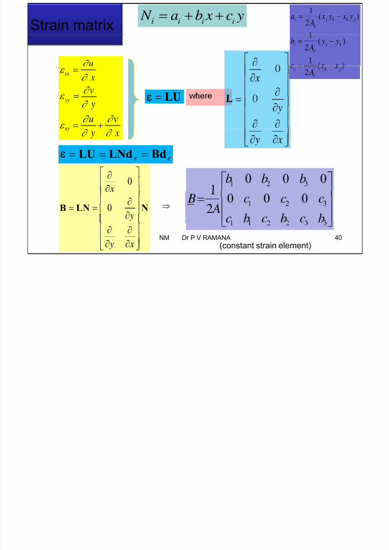
7/25/2019 NM Lecture 6 on 15th Sept 2015.pdf
http://slidepdf.com/reader/full/nm-lecture-6-on-15th-sept-2015pdf 40/76
Strain matrix 2e A
u
( )
21
i j k
e
b y y
A
xx x
v
x
2i k j
e A
yy
y
u v
y
y x
y x BdLNdLU
0
321 000 bbb
0 y
B LN N
321 000
2bcbcbc
ccc A
B
40 y x
(constant strain element)NM Dr P V RAMANA
Element matrices
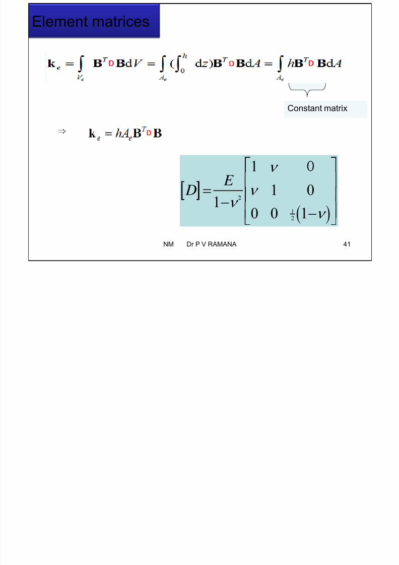
7/25/2019 NM Lecture 6 on 15th Sept 2015.pdf
http://slidepdf.com/reader/full/nm-lecture-6-on-15th-sept-2015pdf 41/76
Element matrices
Constant matrix
1 0 E
D
1
2
10 0 1
41NM Dr P V RAMANA
7/25/2019 NM Lecture 6 on 15th Sept 2015.pdf
http://slidepdf.com/reader/full/nm-lecture-6-on-15th-sept-2015pdf 42/76
1 2 3 2 3 2 2
1[( )( ) ( )( )]
2 N y y x x x x y y
A
7/25/2019 NM Lecture 6 on 15th Sept 2015.pdf
http://slidepdf.com/reader/full/nm-lecture-6-on-15th-sept-2015pdf 43/76
2e
A
2 3 1 1 3 3 1 1 3
1[( ) ( ) ( ) ]
21
e
N x y x y y y x x x y
A
3 1 3 1 3 32 e A
3 1 2 1 1 1 2 2 1
1[( ) ( ) ( ) ] N x y x y y y x x x y
1 2 1 2 1 1
1[( )( ) ( )( )]
2
e
e
y y x x x x y y A
ˆ0u
1 3 5 1 3 5
2 4 6
ˆ ˆ, , 0 , 0 , 0 *( ).
, 0 , 0 , 0 , 0 0
ˆ
u x y N x y N x y N x y u u N N N
v x y N x y N x y N x y
0
u
NM Dr P V RAMANA 43
1 3 5 2 3 3 2 3 1 1 3 1 2 2 1 , , , .
7/25/2019 NM Lecture 6 on 15th Sept 2015.pdf
http://slidepdf.com/reader/full/nm-lecture-6-on-15th-sept-2015pdf 44/76
Constant Strain Triangle (CST) : Simplest 2D finite element

7/25/2019 NM Lecture 6 on 15th Sept 2015.pdf
http://slidepdf.com/reader/full/nm-lecture-6-on-15th-sept-2015pdf 45/76
v3v1
u3
u1
v2
v(x1,y1)
(x3,y3)
y
u22
(x,y)
x
2, 2
• 3 nodes per element
• 2 dofs per node (each node can move in x- and y- directions)• Hence 6 dofs per element
NM Dr P V
RAMANA
45
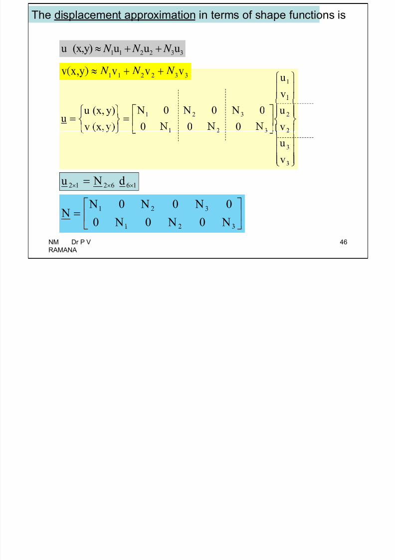
The displacement approximation in terms of shape functions is
7/25/2019 NM Lecture 6 on 15th Sept 2015.pdf
http://slidepdf.com/reader/full/nm-lecture-6-on-15th-sept-2015pdf 46/76
1 1 2 2 3 3u (x,y) u u u N N N
1
v
u1 1 2 2 3 3v x,y v v v
2321
v
u
000
0 N0 N0 N
xv
y)(x,uu
3
vu
166212 d Nu
321
N0 N0 N0
0 N0 N0 N N
NM Dr P V
RAMANA
46
Formula for the shape functions are
cxba
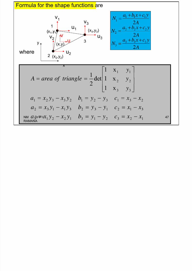
7/25/2019 NM Lecture 6 on 15th Sept 2015.pdf
http://slidepdf.com/reader/full/nm-lecture-6-on-15th-sept-2015pdf 47/76
c xba
yc xba N
A2222
1
v
3
1
u11
(x3,y3)
yc xba N
A2
3333
y
u3v23
(x,y)
vu
where u22 (x2,y2)
11x11
y
x
33
22
x12
y
23132123321
x xcb x xa
x xc y yb y x y xa
12321312213 x xc y yb y x y xa NM Dr P V
RAMANA
47
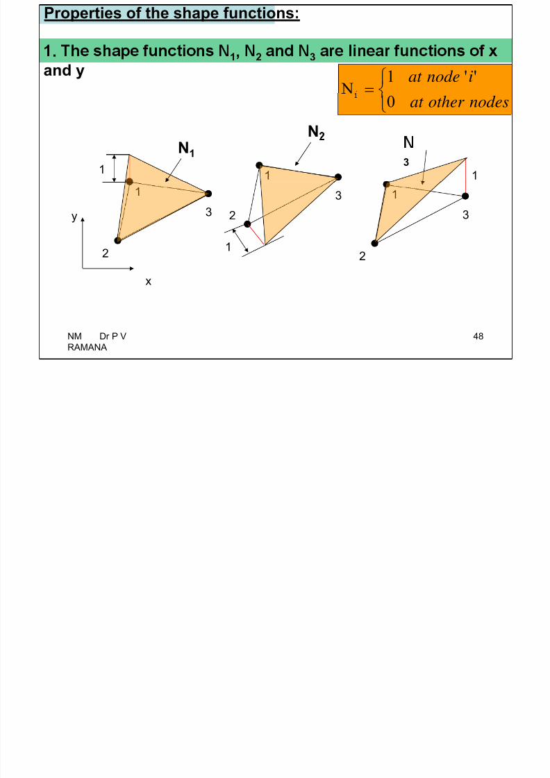
Properties of the shape functions:
7/25/2019 NM Lecture 6 on 15th Sept 2015.pdf
http://slidepdf.com/reader/full/nm-lecture-6-on-15th-sept-2015pdf 48/76
. 1, 2 3
and y inodeat ''1
N
N
nodesother at 0
1
N1
1 13
y 3
1
23
31
21
2
x
NM Dr P V
RAMANA
48
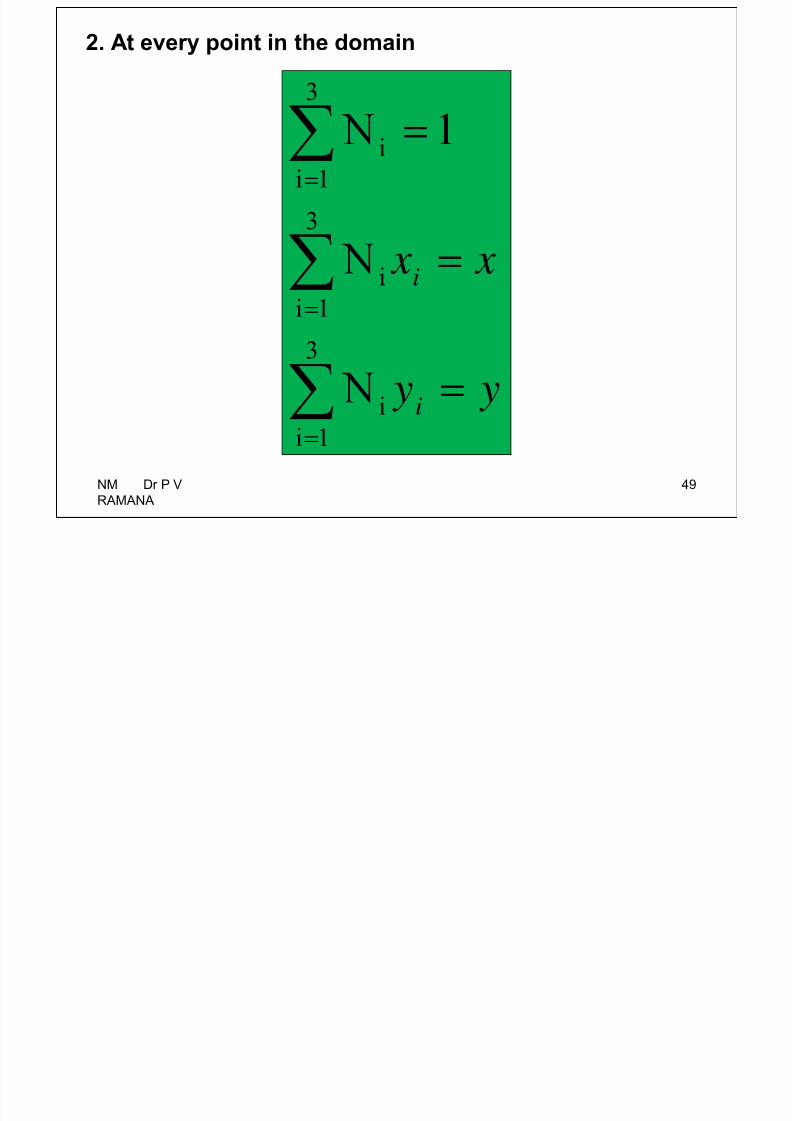
2. At every point in the domain
7/25/2019 NM Lecture 6 on 15th Sept 2015.pdf
http://slidepdf.com/reader/full/nm-lecture-6-on-15th-sept-2015pdf 49/76
3
1i
i
3
i1i i
3
i
1i
i
NM Dr P V
RAMANA
49
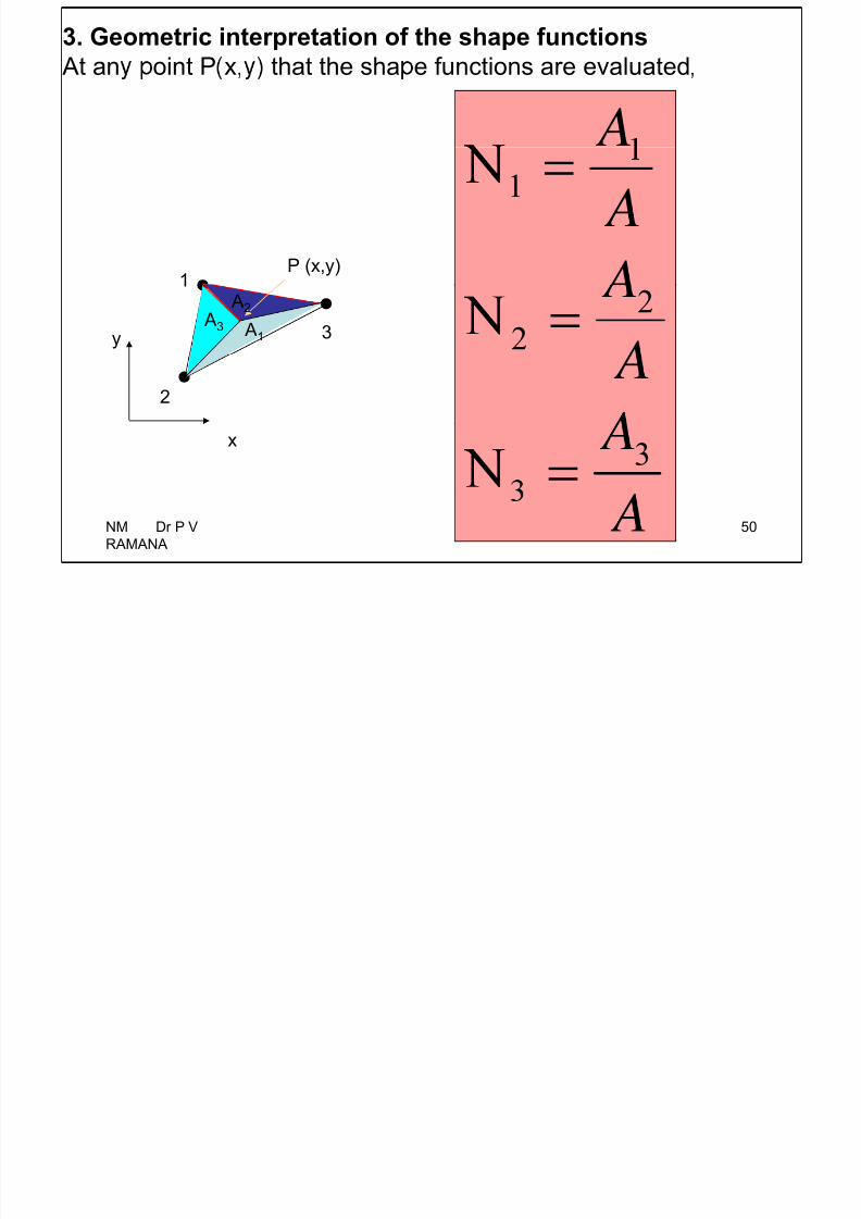
3. Geometric interpretation of the shape functions
At an oint P x that the sha e functions are evaluated
7/25/2019 NM Lecture 6 on 15th Sept 2015.pdf
http://slidepdf.com/reader/full/nm-lecture-6-on-15th-sept-2015pdf 50/76
At an oint P x that the sha e functions are evaluated
A1
1P (x,y)
y 3 A1 A3
A2 22
2
x3
NM Dr P V
RAMANA
50
Approximation of the strains
u
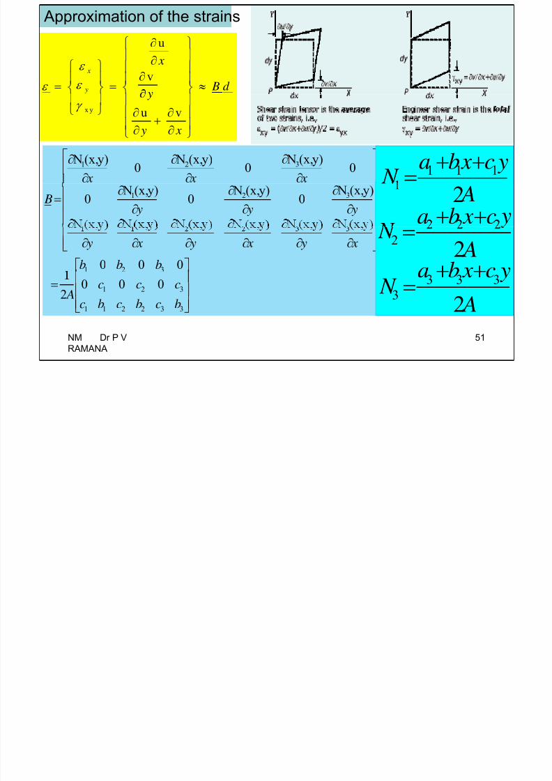
7/25/2019 NM Lecture 6 on 15th Sept 2015.pdf
http://slidepdf.com/reader/full/nm-lecture-6-on-15th-sept-2015pdf 51/76
u
v x
y
x
B d
x y u v
y x
321 0y)(x, N
0y)(x, N
0y)(x, N
x x x yc xba 111
321 y)(x, N
0
y)(x, N
0
y)(x, N
0 y y y Bc xba 2
321 000 bbb
x y x y x y A22
332211
321 0002
bcbcbc
ccc A
A N
2
3333
NM Dr P V
RAMANA
51
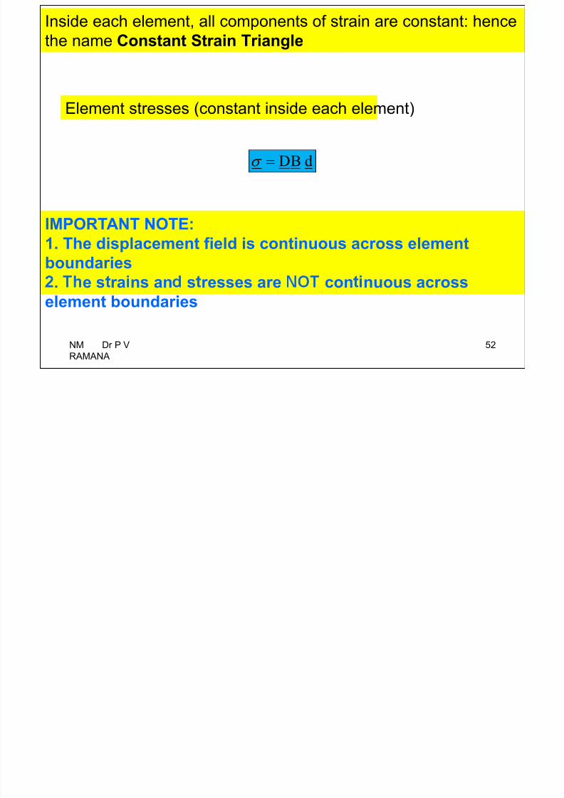
Inside each element, all components of strain are constant: hence
the name Constant Strain Triangle
7/25/2019 NM Lecture 6 on 15th Sept 2015.pdf
http://slidepdf.com/reader/full/nm-lecture-6-on-15th-sept-2015pdf 52/76
g
Element stresses (constant inside each element)
dBD
IMPORTANT NOTE:
1. The displacement field is continuous across element
boundaries. e s ra ns an s resses are con nuous across
element boundaries
NM Dr P V
RAMANA
52
Element stiffness matrix
321
321
000
000
2
1ccc
bbb
B

7/25/2019 NM Lecture 6 on 15th Sept 2015.pdf
http://slidepdf.com/reader/full/nm-lecture-6-on-15th-sept-2015pdf 53/76
2
eV k dVBDBT
t 332211 ccc
1 0
Since B is constant
2
1
1 01
0 0 1
D
At k eV BDBdVBDBTT
t=thickness of the element A=surface area of the element
T T
S
eT
b
e
f
S S
f
V
NM Dr P V
RAMANA
53
Element nodal load vector due to body forces
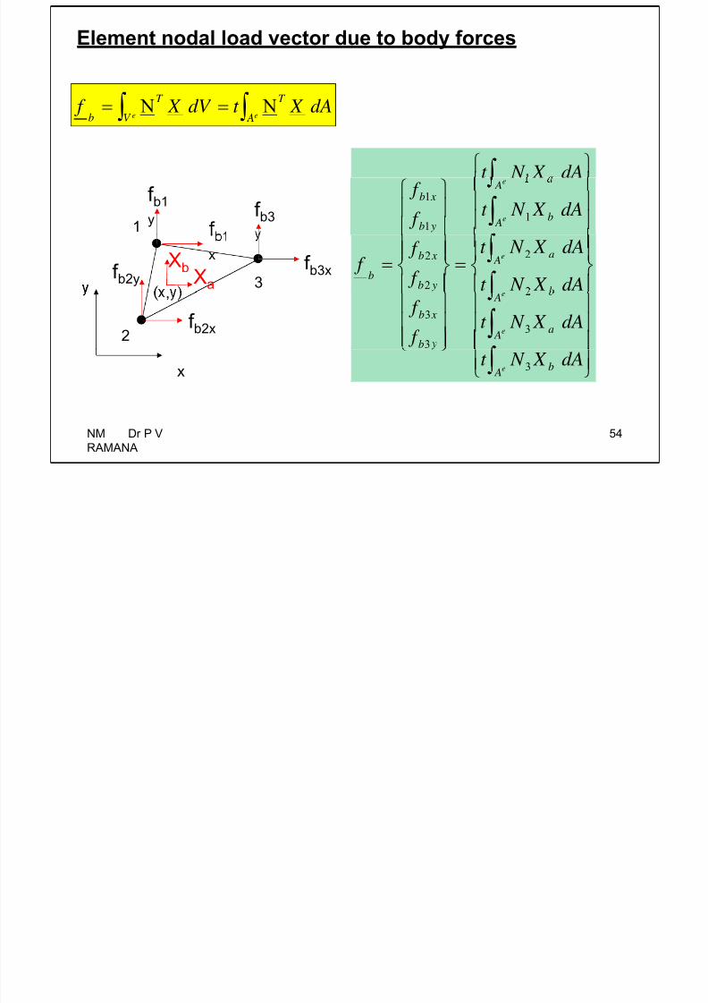
7/25/2019 NM Lecture 6 on 15th Sept 2015.pdf
http://slidepdf.com/reader/full/nm-lecture-6-on-15th-sept-2015pdf 54/76
ee
T T
bdA X t dV X f N N
dA X N t
e
e
A b
A
yb
xb
dA X N t f
f
11
1
f b3
f b1
y1
e A a
yb
xbb
dA X N t
dA X N t
f
f f 2
2
2f b3xxf b2y 3
XbXa
e
e
A a
A
b
xbdA X N t
f
f 3
3
3f b2x
2
,
e A b dA X N t 3x
NM Dr P V
RAMANA
54
LINEAR RECTANGULAR ELEMENTS
7/25/2019 NM Lecture 6 on 15th Sept 2015.pdf
http://slidepdf.com/reader/full/nm-lecture-6-on-15th-sept-2015pdf 55/76
• Non-constant strain matrix
1 2 3 4
• More accurate representation of stress and strain
• Regular shape makes formulation easy
55NM Dr P V RAMANA
7/25/2019 NM Lecture 6 on 15th Sept 2015.pdf
http://slidepdf.com/reader/full/nm-lecture-6-on-15th-sept-2015pdf 56/76
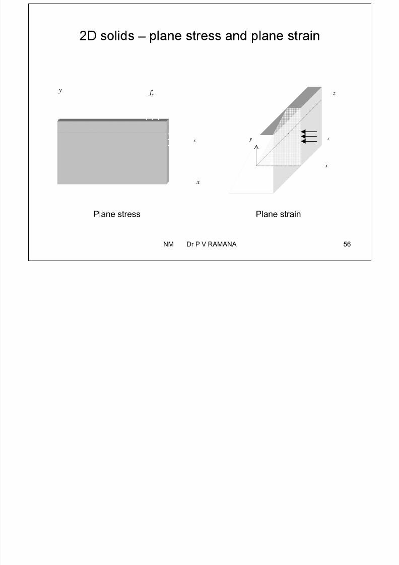
–
f y y z
x y x
x
x
Plane stress Plane strain
56NM Dr P V RAMANA
Rectangular Element:
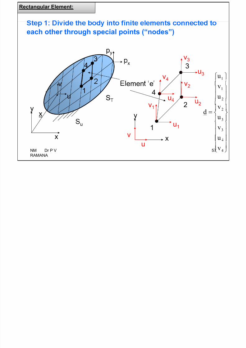
7/25/2019 NM Lecture 6 on 15th Sept 2015.pdf
http://slidepdf.com/reader/full/nm-lecture-6-on-15th-sept-2015pdf 57/76
each other through special points (“nodes”)
py
3v
3x4 3u3
v4 1u
Su
v emen e
1 4u
v2
2
1
u
v
yx
y
2 2v1
3
2
u
vd
x
u
xv
1u1
3
u
v
u 4vNM Dr P V
RAMANA
57
Element Formulation

7/25/2019 NM Lecture 6 on 15th Sept 2015.pdf
http://slidepdf.com/reader/full/nm-lecture-6-on-15th-sept-2015pdf 58/76
Three approaches for generating shape
“Interpolation approach”:
-• Works best for small numbers of d.o.f.
“Direct approach”:ore geome r c me o
Works best for higher-order elements
“Area based approach”:
NM Dr P V RAMANA 58Large structures or nearly volumetric Works best for higher-order elements
Basics:
8 d.o.f. total 8 sha e functions3
u3
v3
v
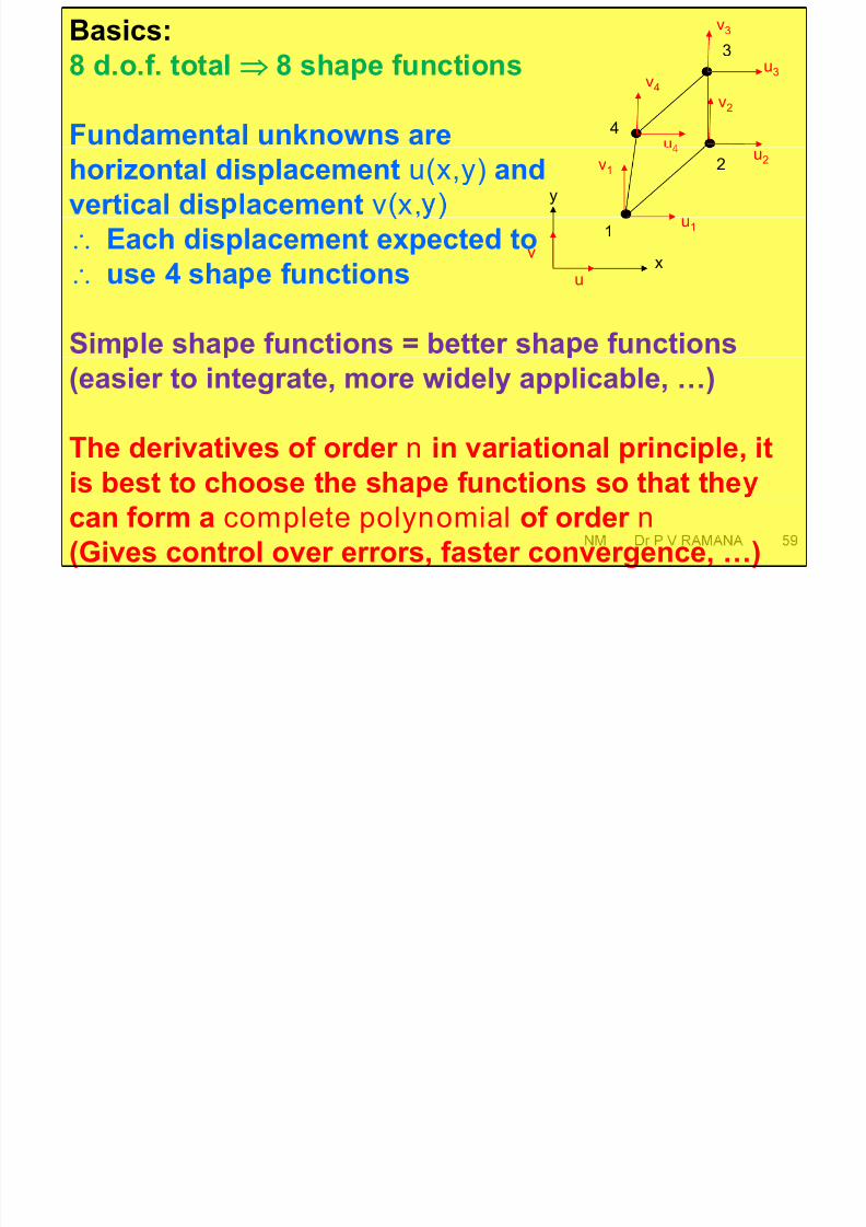
7/25/2019 NM Lecture 6 on 15th Sept 2015.pdf
http://slidepdf.com/reader/full/nm-lecture-6-on-15th-sept-2015pdf 59/76
Fundamental unknowns are 4u
v4
v2
horizontal displacement u(x,y) and
vertical dis lacement v x,
y
2u2v1
Each displacement expected to
use 4 sha e functionsx
v
u
1u1
Sim le sha e functions = better sha e functions
(easier to integrate, more widely applicable, …)
The derivatives of order n in variational principle, it
is best to choose the sha e functions so that the
NM Dr P V RAMANA 59can form a complete polynomial of order n(Gives control over errors, faster convergence, …)
Element Formulation

7/25/2019 NM Lecture 6 on 15th Sept 2015.pdf
http://slidepdf.com/reader/full/nm-lecture-6-on-15th-sept-2015pdf 60/76
“Interpolation approach”:st , ,
xya ya xaa y xv xya ya xaa y xu 87654321 ),(;),(
– At each node, require u(xi,yi) = ui and v(xi,yi) = vi :
xaa xaav xaa xaau
228272652224232212 ; y xa ya xaav y xa ya xaau
448474654444434214
338373653334333213
;
;
y xa ya xaav y xa ya xaau
y xa ya xaav y xa ya xaau
NM Dr P V
RAMANA
60
Element Formulation; yxayaxaavyxayaxaau
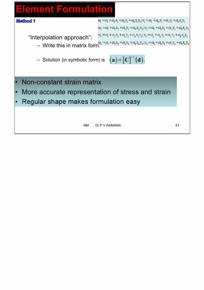
7/25/2019 NM Lecture 6 on 15th Sept 2015.pdf
http://slidepdf.com/reader/full/nm-lecture-6-on-15th-sept-2015pdf 61/76
228272652224232212
118171651114131211
;
;
y xa ya xaav y xa ya xaau
y xa ya xaav y xa ya xaau
“Interpolation approach”:
– Write this in matrix form:448474654444434214
338373653334333213
; y xa ya xaav y xa ya xaau
– Solution (in symbolic form) is 1
.a C d
• Non-constant strain matrix
• More accurate representation of stress and strain
•
NM Dr P V RAMANA 61
Element Formulation
)()(

7/25/2019 NM Lecture 6 on 15th Sept 2015.pdf
http://slidepdf.com/reader/full/nm-lecture-6-on-15th-sept-2015pdf 62/76
“Interpolation approach”: xya ya xaa y xv xya ya xaa y xu87654321
),(;),(
– ow, rewr e n erpo a on unc ons n ma r x vec or orm:
1
.
xya ya xaa y xv xya ya xaa y xu ),(;),( 87654321
aP y xu xu ),()(
–1
,
.
N x
NM Dr P V RAMANA 62
7/25/2019 NM Lecture 6 on 15th Sept 2015.pdf
http://slidepdf.com/reader/full/nm-lecture-6-on-15th-sept-2015pdf 63/76
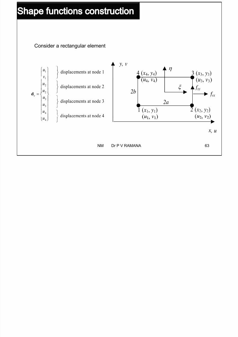
Consider a rectangular element
, v
3 ( x3, y3)4 ( x4, y4)
1 displacements at node 1u
v
u3, v3
sy
sx
4, 4
2b 2
2 displacements at node 2
e
u
u
d
1 ( x1, y1) 2 ( x2, y2)
2a3
3
4
displacements at node 3
dis lacements at node 4
u
u
, u
, ,4u
63NM Dr P V RAMANA
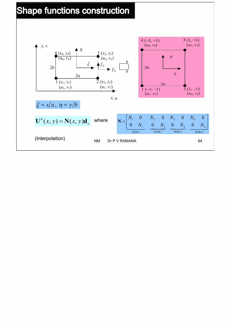
7/25/2019 NM Lecture 6 on 15th Sept 2015.pdf
http://slidepdf.com/reader/full/nm-lecture-6-on-15th-sept-2015pdf 64/76
, v
3 ( x3, y3)4 ( x4, y4)
,
(u3, v3)
, +
(u4, v4)
3, 3
sy
sx
4, 4
2b
2b
1 ( x1, y1)(u1, v1)
2 ( x2, y2) (u2, v2)
1 (1, 1)
u v
2 (1, 1)
u2, v2
2a
, u
, b ya x
( , ) ( , )h
e x y x yU N d
31 2 4
31 2 4
00 0 0
00 0 0
N N N N
N N N N
N
where
NM Dr P V RAMANA 64
(Interpolation)
Summary: For each element
Rectangular Element:
Displacement approximation in terms of shape functions

7/25/2019 NM Lecture 6 on 15th Sept 2015.pdf
http://slidepdf.com/reader/full/nm-lecture-6-on-15th-sept-2015pdf 65/76
Displacement approximation in terms of shape functions
d Nu
Strain approximation in terms of strain-displacement matrix
Stress approximation
dBε
dBD
e
V
k dVBDBT
Element nodal load vector
T T
S
eT
b
e
f
S
f
V
NM Dr P V
RAMANA
65
Lagrange family
Serendipity family
Second Approach
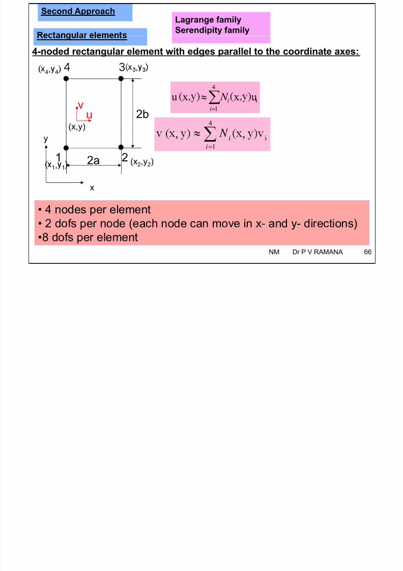
7/25/2019 NM Lecture 6 on 15th Sept 2015.pdf
http://slidepdf.com/reader/full/nm-lecture-6-on-15th-sept-2015pdf 66/76
4-noded rectangular element with edges parallel to the coordinate axes:,
4, 4
4
uxxu N
(x,y)
vu 2b
1i
4
y
(x2,y2)1 22a
1
i,,
i
i
x
,
• 4 nodes per element
• 2 dofs per node (each node can move in x- and y- directions)
•8 dofs per element NM Dr P V RAMANA 66
Generation of N1:2 x x
1xx

7/25/2019 NM Lecture 6 on 15th Sept 2015.pdf
http://slidepdf.com/reader/full/nm-lecture-6-on-15th-sept-2015pdf 67/76
y 21 x x
has the property
34l1(y)
0)(
1)(
21
11
xl
xl
2b Similarly
41
41 )(
y y
y y yl
x
1 2
2a
N1
has the property1)( 11 yl
l1(x)
10)( 41 yl
Hence choose the shape function at node 1 a
4242
111
1)()( y y x x
y y x x yl xl N
4121 a y y x x
NM Dr P V RAMANA 67
7/25/2019 NM Lecture 6 on 15th Sept 2015.pdf
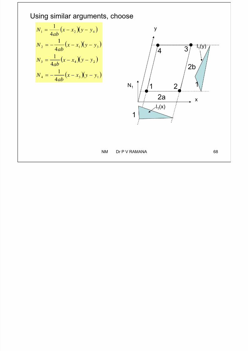
http://slidepdf.com/reader/full/nm-lecture-6-on-15th-sept-2015pdf 68/76
Second Approach
b ya xab
y y x xab
N 4
1
4
1421
by
a xyyxxN

7/25/2019 NM Lecture 6 on 15th Sept 2015.pdf
http://slidepdf.com/reader/full/nm-lecture-6-on-15th-sept-2015pdf 69/76
Lagrange familySerendi it famil 11 b ya x
b y
ab
y y x x
ab
N
144
312
Lagrange family
1144243
ab y y
ab
b ya x
y y x x N
11
134
4-noded rectangle
y
In local coordinate system
a a
12
b b xaab
N
41
y
l1(
x
b
yb xa
ab
))((
42
2b
y
3 4
yb xa N
ab
))((
43
1 22a
N1 1
ab4NM Dr P V RAMANA 69l1(x)1
1 Polynomial completeness
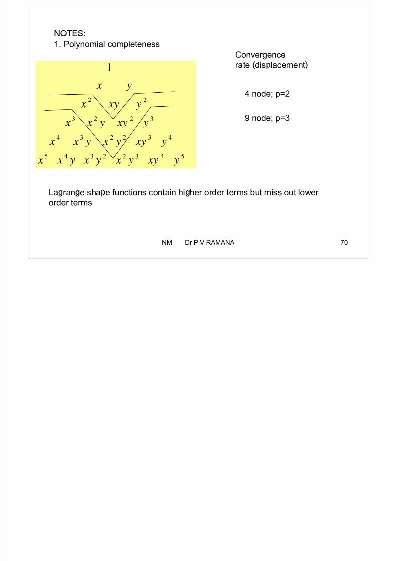
7/25/2019 NM Lecture 6 on 15th Sept 2015.pdf
http://slidepdf.com/reader/full/nm-lecture-6-on-15th-sept-2015pdf 70/76
1. Polynomial completeness
Convergencerate dis lacement
y x4 node; p=2
3223 y xy y x x
y xy x9 node; p=3
54322345
432234
x x x x x y xy y x y x x
La ran e sha e functions contain hi her order terms but miss out lowerorder terms
NM Dr P V RAMANA 70
Properties of the shape functions:

7/25/2019 NM Lecture 6 on 15th Sept 2015.pdf
http://slidepdf.com/reader/full/nm-lecture-6-on-15th-sept-2015pdf 71/76
1. The shape functions N1, N2 , N3 and N4 are bilinearfunctions of x and
2. Kronecker delta property
nodesother at
inodeat y x
0
''1),( N i
3. Completeness
y
a a 12
4
1i
i 1 N x
x x i
4
1i
i N 3 4
y y i 1i
i N NM Dr P V RAMANA 71
3. Along lines parallel to the x- or y-axes, the shape functions
are linear. But along any other line they are nonlinear.

7/25/2019 NM Lecture 6 on 15th Sept 2015.pdf
http://slidepdf.com/reader/full/nm-lecture-6-on-15th-sept-2015pdf 72/76
4. An element shape function related to a specific nodal point
point.
5. The displacement field is continuous across elements
. e s ra ns an s resses are no cons an w n an
element nor are they continuous across element boundaries.
y
a a12
x
b
NM Dr P V RAMANA 723 4
The strain-displacement relationship
4214
1 y y x x
ab N
34
2
l1(y)
x
3124
1 y y x x
ab N b
N
1

7/25/2019 NM Lecture 6 on 15th Sept 2015.pdf
http://slidepdf.com/reader/full/nm-lecture-6-on-15th-sept-2015pdf 73/76
xy
y
2434
1
4
y y x xab
N
ab
x1 22
N1
1
1
1
4321
v
u
y)(x,y)(x, Ny)(x,y)(x, N
1344
1 y y x x
ab N a
1
1
3
2
2
4321
u
v
u
y)(x, N0
y)(x, N0
y)(x, N0
y)(x, N0
y y y y
x x x x
4
3
B
44332211
u
vy)(x, Ny)(x, Ny)(x, Ny)(x, Ny)(x, Ny)(x, Ny)(x, Ny)(x, N
x y x y x y x y
4
y y y y y y y y 1234 0000
y y x x y y x x y y x x y y x x
x x x x x x x xab
B
13243142
3412 00004
o ce a e s ra ns an ence s resses are cons an w n an
element NM Dr P V RAMANA 73
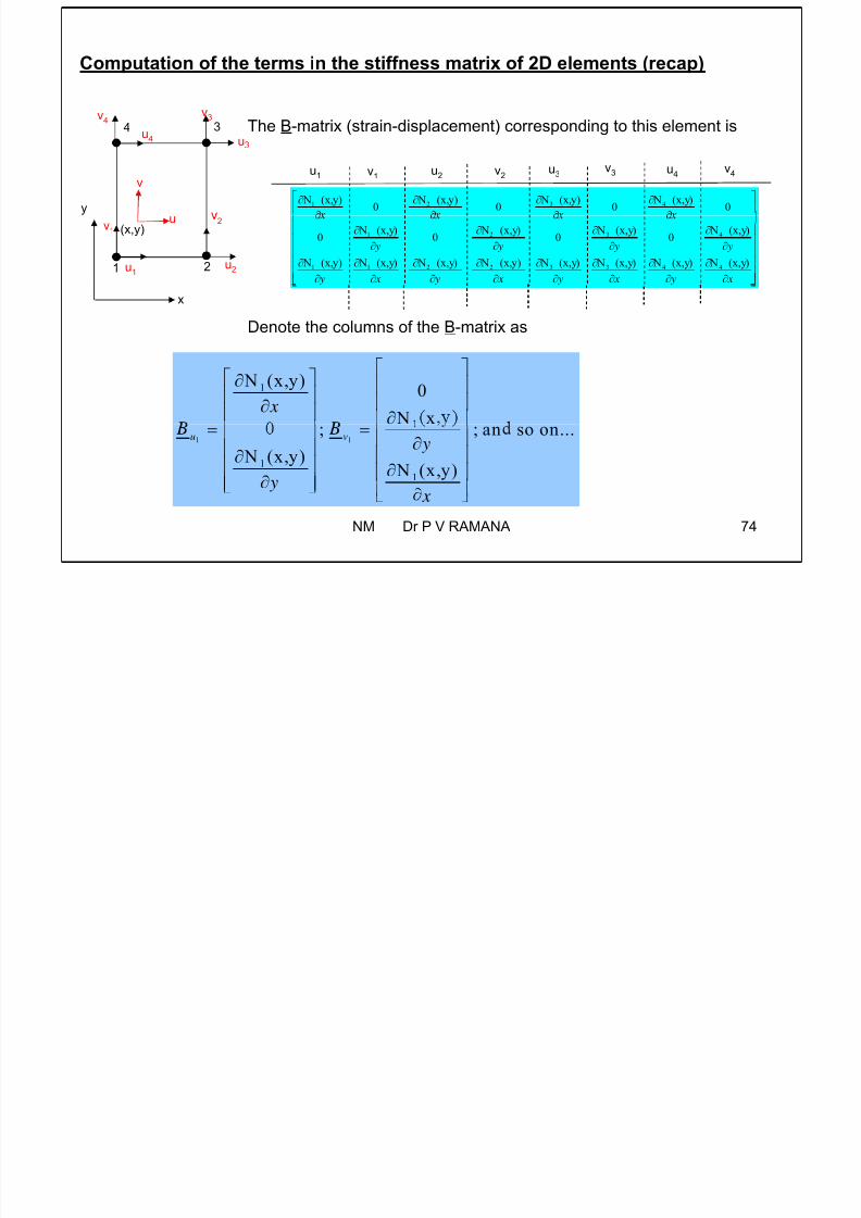
Computation of the terms in the stiffness matrix of 2D elements (recap)
7/25/2019 NM Lecture 6 on 15th Sept 2015.pdf
http://slidepdf.com/reader/full/nm-lecture-6-on-15th-sept-2015pdf 74/76
The B-matrix (strain-displacement) corresponding to this element is34v4 v3
uu4
y
v
1 2 3 4 N (x,y) N (x,y) N (x,y) N (x,y)0 0 0 0
u1 v1u2 v2
u3 u4v3 v4
(x,y) u
1 2
2v1
u1u2
1 2 3 4
1 1 2 2 3 3 4 4
N (x,y) N (x,y) N (x,y) N (x,y)0 0 0 0
N (x,y) N (x,y) N (x,y) N (x,y) N (x,y) N (x,y) N (x,y) N (x,y)
y y y y
y x y x y x y x
Denote the columns of the B-matrix as
x
1 N (x,y)0
N x x
1 1
1
1
; ; an so on...
N (x,y) N (x,y)
u v y
y
x
NM Dr P V RAMANA 74
The stiffness matrix corresponding to this element is
eV
k dVBDB which has the following form
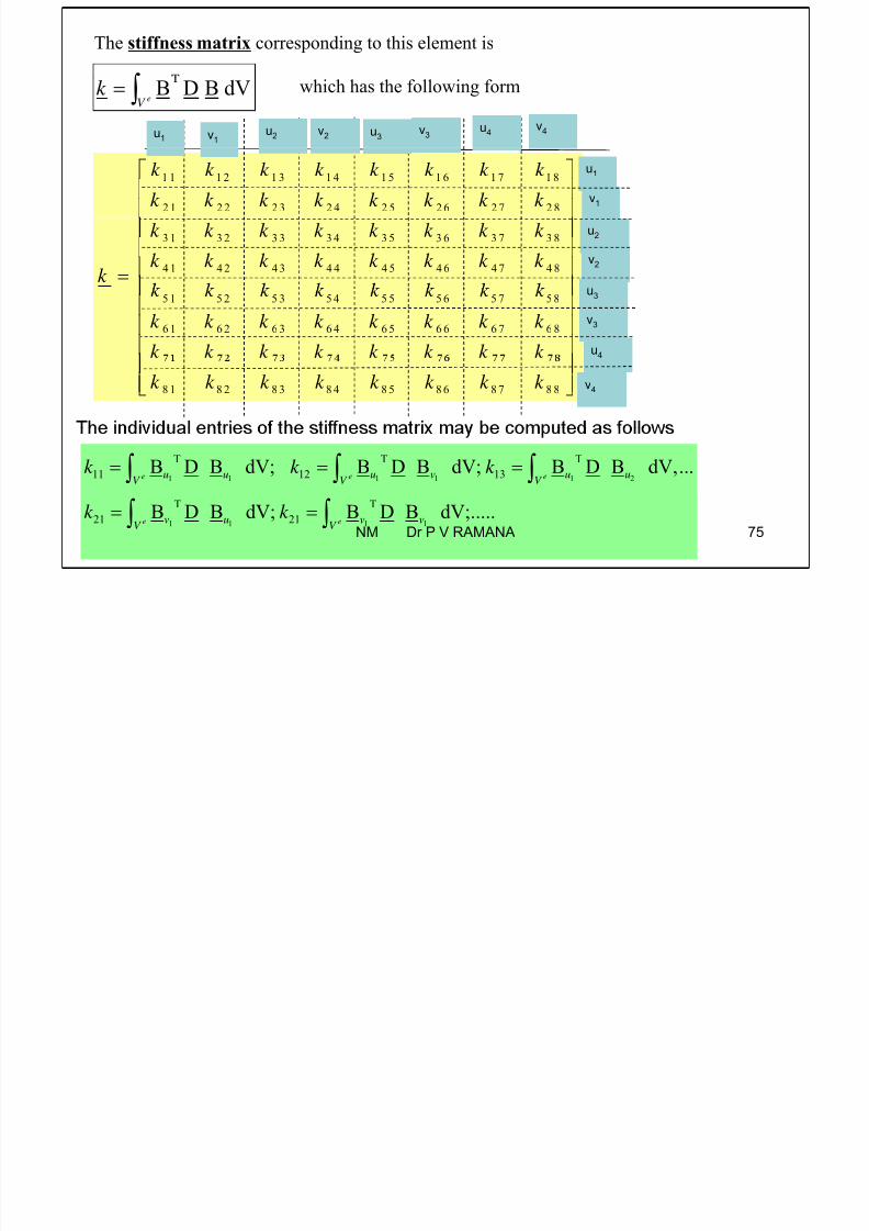
7/25/2019 NM Lecture 6 on 15th Sept 2015.pdf
http://slidepdf.com/reader/full/nm-lecture-6-on-15th-sept-2015pdf 75/76
V
u1 v1u2 v2 u3
u4v3v4
1 1 1 2 1 3 1 4 1 5 1 6 1 7 1 8
2 1 2 2 2 3 2 4 2 5 2 6 2 7 2 8
k k k k k k k k
k k k k k k k k
u1
v1
3 1 3 2 3 3 3 4 3 5 3 6 3 7 3 8
4 1 4 2 4 3 4 4 4 5 4 6 4 7 4 8
k k k k k k k k
k k k k k k k k k
u2
v2
5 1 5 2 5 3 5 4 5 5 5 6 5 7 5 8
6 1 6 2 6 3 6 4 6 5 6 6 6 7 6 8k k k k k k k k k k k k k k k k
u3
u4
v3
8 1 8 2 8 3 8 4 8 5 8 6 8 7 8 8k k k k k k k k v4
1 1 1 1 1 2
T T T
11 12 13B D B dV; B D B dV; B D B dV,...e e eu u u v u u
V V V k k k
1 1 1 1
T T
21 21B D B dV; B D B dV;.....e ev u v v
V V
k k
NM Dr P V RAMANA 75

7/25/2019 NM Lecture 6 on 15th Sept 2015.pdf
http://slidepdf.com/reader/full/nm-lecture-6-on-15th-sept-2015pdf 76/76
76NM Dr P V RAMANA