Embed Size (px)
Citation preview
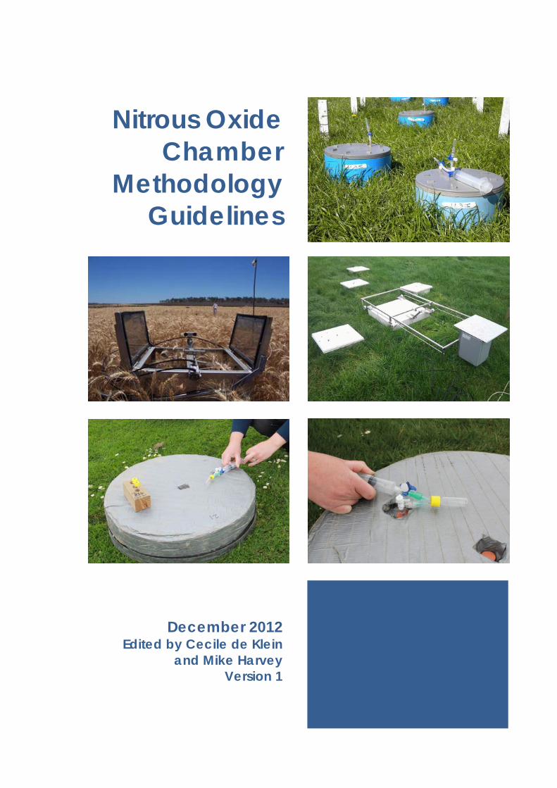
Nitrous Oxide Chamber
Methodology Guidelines
December 2012 Edited by Cecile de Klein
and Mike Harvey Version 1

2 | NITROUS OXIDE CHAMBER METHODOLOGY GUIDELINES – Version 1
Acknowledgements This manual has been commissioned by the New Zealand Government to support the goals and objectives of the Global Research Alliance on Agricultural Greenhouse Gases, but its contents rely heavily on the contributions from individual scientists in Alliance member countries. The participation of these scientists and their institutions is gratefully acknowledged, and warm thanks are extended for their contribution to this document.
We thank the two international peer reviewers for their expert review and invaluable comments on these Guidelines and Dave Hansford for professional editorial services.
Publisher details Ministry for Primary Industries Pastoral House, 25 The Terrace PO Box 2526, Wellington 6140, New Zealand Tel: +64 4 894 0100 or 0800 00 83 33 Web: www.mpi.govt.nz Copies can be downloaded in a printable pdf format from http://www.globalresearchalliance.org The document and material contained within will be free to download and reproduce for educational or non-commercial purposes without any prior written permission from the authors of the individual chapters. Authors must be duly acknowledged and material fully referenced. Reproduction of the material for commercial or other reasons is strictly prohibited without the permission of the authors. ISBN 978-0-478-40584-2 (print) ISBN 978-0-478-40585-9 (online)
Disclaimer While every effort has been made to ensure the information in this publication is accurate, the Livestock Research Group of the Global Research Alliance on Agricultural Greenhouse Gases does not accept any responsibility or liability for error of fact, omission, interpretation or opinion that may be present, nor for the consequences of any decisions based on this information. Any view or opinion expressed does not necessarily represent the view of the Livestock Research Group of the Global Research Alliance on Agricultural Greenhouse Gases.
Contents | 3
Nitrous Oxide Chamber Methodology Guidelines Version 1
Editors C. A. M. de Klein AgResearch, Invermay Research Centre, Private Bag 50034, Mosgiel, New Zealand [email protected]
M. J. Harvey NIWA, Private Bag 14-901, Kilbirnie, Wellington, New Zealand [email protected]
Nitrous Oxide Chamber Methodology Guidelines Cecile de Klein & Mike Harvey ( Eds )
1. Introduction – Cecile de Klein & Mike Harvey (New Zealand)
2. Chamber design – Tim Clough (New Zealand) et al.
3. Deployment protocol – al.
4. Air sample collection, storage and analysis – Frank Kelliher (New Zealand) et al.
5. Automated GHG measurement in the field – Peter Grace (Australia) et al.
6. Data analysis considerations – Rod Venterea (US) et al.
7. How to report your experimental data – Marta Alfaro (Chile) et al.
8. Health and safety considerations – David Chadwick (UK) et al.
Philippe Rochette (Canada) et


Chapter 6: Data Analysis Considerations | 95
6 DATA ANALYSIS CONSIDERATIONS
Author for correspondence - Email: [email protected]
R.T. Venterea1, T.BParkin2, L. Cardenas3, S.O. Petersen4 & A.R. Pedersen5.
1USDA-ARS, Soil and Water Management Research Unit, 1991 Upper Buford Cir., 439 Borlaug Hall, St. Paul, MN 55108. 2National Laboratory for Agriculture and the Environment, 2110 University Boulevard, Ames, Iowa 50011-3120. 3Rothamsted Research, North Wyke, Okehampton, Devon, EX20 2SB, United Kingdom. 4Department of Agroecology and Environment, Faculty of Agricultural Sciences, University of Aarhus, PO Box 50, DK-8830 Tjele, Denmark. 5Department of Genetics and Biotechnology, Faculty of Agricultural Sciences, University of Aarhus, PO Box 50, DK-8830 Tjele, Denmark.
96 | NITROUS OXIDE CHAMBER METHODOLOGY GUIDELINES – Version 1
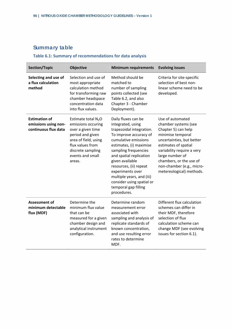
Summary table Table 6.1: Summary of recommendations for data analysis
Section/Topic Objective Minimum requirements Evolving issues
Selecting and use of a flux calculation method
Selection and use of most appropriate calculation method for transforming raw chamber headspace concentration data into flux values.
Method should be matched to number of sampling points collected (see Table 6.2, and also Chapter 3 - Chamber Deployment).
Criteria for site-specific selection of best non-linear scheme need to be developed.
Estimation of emissions using non-continuous flux data
Estimate total N2O emissions occuring over a given time period and given area of field, using flux values from discrete sampling events and small areas.
Daily fluxes can be integrated, using trapezoidal integration. To improve accuracy of cumulative emissions estimates, (i) maximise sampling frequencies and spatial replication given available resources, (ii) repeat experiments over multiple years, and (iii) consider using spatial or temporal gap filling procedures.
Use of automated chamber systems (see Chapter 5) can help minimise temporal uncertainties, but better estimates of spatial variability require a very large number of chambers, or the use of non-chamber (e.g., micro-metereological) methods.
Assessment of minimum detectable flux (MDF)
Determine the minimum flux value that can be measured for a given chamber design and analytical instrument configuration.
Determine random measurement error associated with sampling and analysis of replicate standards of known concentration, and use resulting error rates to determine MDF.
Different flux calculation schemes can differ in their MDF, therefore selection of flux calculation scheme can change MDF (see evolving issues for section 6.1).
Chapter 6: Data Analysis Considerations | 97
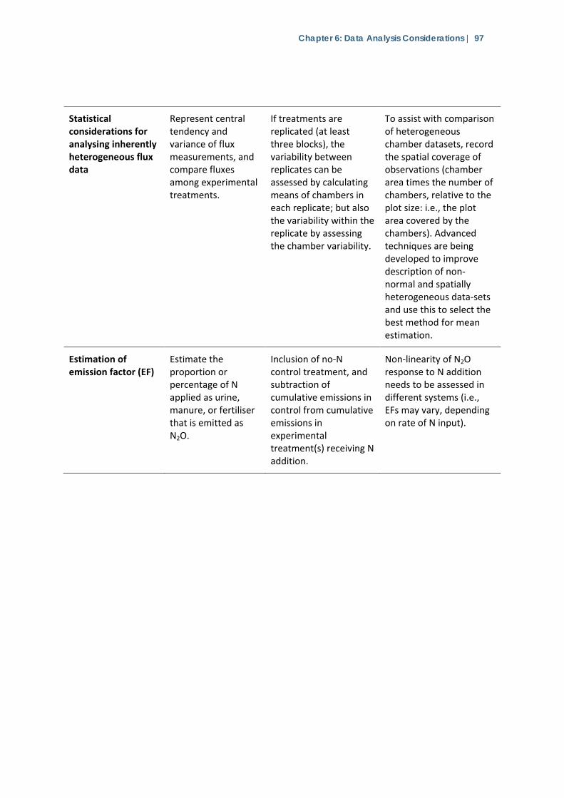
Statistical considerations for analysing inherently heterogeneous flux data
Represent central tendency and variance of flux measurements, and compare fluxes among experimental treatments.
If treatments are replicated (at least three blocks), the variability between replicates can be assessed by calculating means of chambers in each replicate; but also the variability within the replicate by assessing the chamber variability.
To assist with comparison of heterogeneous chamber datasets, record the spatial coverage of observations (chamber area times the number of chambers, relative to the plot size: i.e., the plot area covered by the chambers). Advanced techniques are being developed to improve description of non-normal and spatially heterogeneous data-sets and use this to select the best method for mean estimation.
Estimation of emission factor (EF)
Estimate the proportion or percentage of N applied as urine, manure, or fertiliser that is emitted as N2O.
Inclusion of no-N control treatment, and subtraction of cumulative emissions in control from cumulative emissions in experimental treatment(s) receiving N addition.
Non-linearity of N2O response to N addition needs to be assessed in different systems (i.e., EFs may vary, depending on rate of N input).
98 | NITROUS OXIDE CHAMBER METHODOLOGY GUIDELINES – Version 1
6.1 Selection and use of a flux calculation (FC) method The first step in any analysis of chamber N2O data is to calculate the flux from the basic chamber concentration versus time data. It is well documented that selection of a FC scheme can substantially alter the magnitude of flux estimates, as well as the sensitivity to detecting fluxes (Parkin et al. 2012). Levy et al. (2011) concluded that selection of a FC method was the largest single source of uncertainty in flux estimates from individual chambers.
The various FC schemes differ in their theoretical basis, numerical requirements and potentially, their accuracy and precision. Presently, there is no single clear or perfect choice for the ‘best’ FC scheme for all applications, and it is not our intention to make a specific recommendation. Our objectives here are instead to summarise the key attributes – and potential limitations – of the most widely used FC schemes from both practical and theoretical perspectives, so that users can make informed decisions for particular applications. We will also make some recommendations on FC scheme selection, based on the number of sampling points collected during each deployment period (DP). This approach is taken because the number of sampling points largely determines the overall suitability of the different schemes.
6.1.1 Basic considerations Non-steady-state chambers rely on the accumulation of the gas of interest (in our case, N2O) within an open-bottom chamber placed on the soil surface. The presence of the chamber is likely to affect gas diffusion: in theory, accumulation of N2O in the chamber immediately suppresses the vertical gradient in N2O concentration, thereby suppressing the flux below its pre-deployment value (F0) (Anthony et al. 1995).
Chamber placement may also create horizontal gradients in gas concentration, as well as pressure gradients that may further alter the flux (Mathias et al. 1978; Pedersen et al. 2010). The net result of at least the first two of these effects is that they lead to non-linearity in the relationship between chamber concentration (C) and time (t) after deployment, such that the maximum value of the slope (dC/dt) occurs immediately after chamber placement and decreases over time. This alteration in the slope complicates the estimation of F0, and selection of a FC scheme. While F0 will be best represented by the slope value occurring immediately after chamber placement, determining the initial value of dC/dt can be problematic in practice.
Chapter 6: Data Analysis Considerations | 99
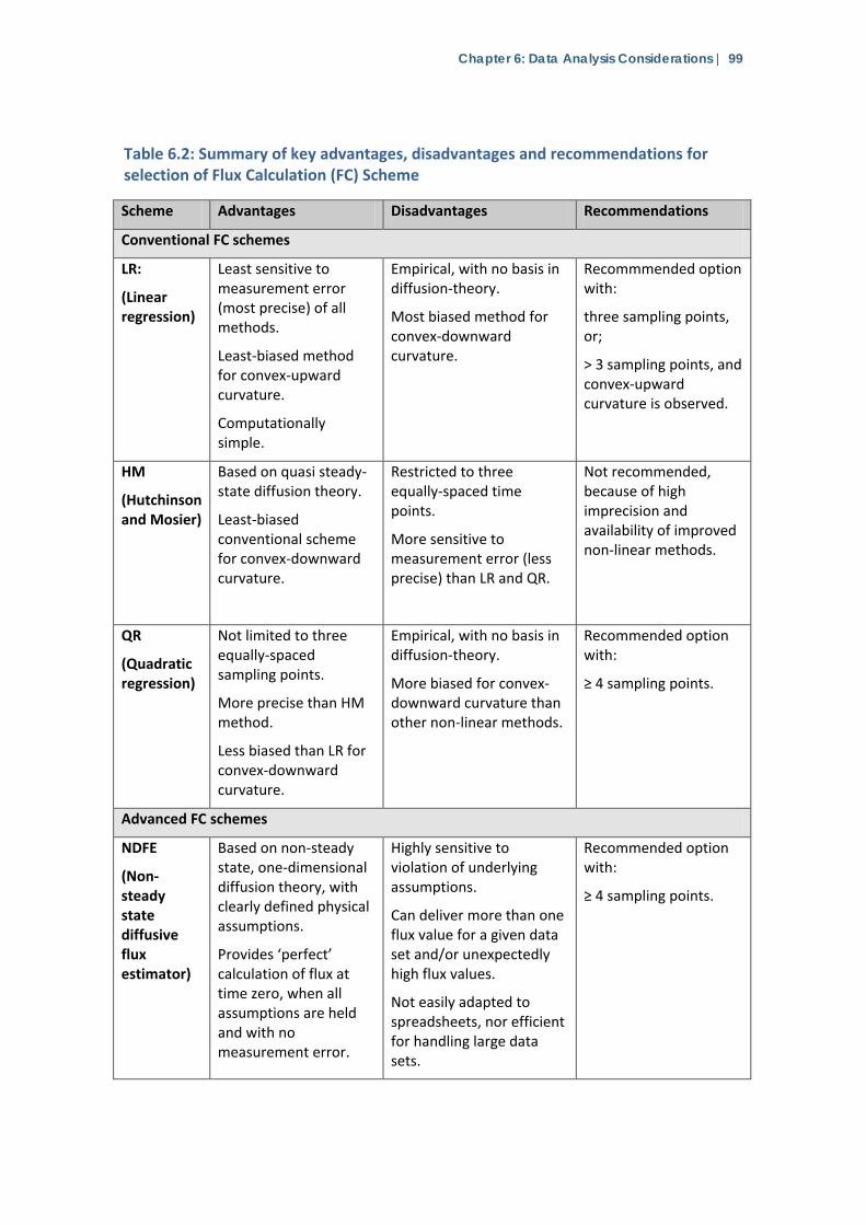
Table 6.2: Summary of key advantages, disadvantages and recommendations for selection of Flux Calculation (FC) Scheme
Scheme Advantages Disadvantages Recommendations
Conventional FC schemes
LR:
(Linear regression)
Least sensitive to measurement error (most precise) of all methods.
Least-biased method for convex-upward curvature.
Computationally simple.
Empirical, with no basis in diffusion-theory.
Most biased method for convex-downward curvature.
Recommmended option with:
three sampling points, or;
> 3 sampling points, and convex-upward curvature is observed.
HM
(Hutchinson and Mosier)
Based on quasi steady-state diffusion theory.
Least-biased conventional scheme for convex-downward curvature.
Restricted to three equally-spaced time points.
More sensitive to measurement error (less precise) than LR and QR.
Not recommended, because of high imprecision and availability of improved non-linear methods.
QR
(Quadratic regression)
Not limited to three equally-spaced sampling points.
More precise than HM method.
Less biased than LR for convex-downward curvature.
Empirical, with no basis in diffusion-theory.
More biased for convex-downward curvature than other non-linear methods.
Recommended option with:
≥ 4 sampling points.
Advanced FC schemes
NDFE
(Non-steady state diffusive flux estimator)
Based on non-steady state, one-dimensional diffusion theory, with clearly defined physical assumptions.
Provides ‘perfect’ calculation of flux at time zero, when all assumptions are held and with no measurement error.
Highly sensitive to violation of underlying assumptions.
Can deliver more than one flux value for a given data set and/or unexpectedly high flux values.
Not easily adapted to spreadsheets, nor efficient for handling large data sets.
Recommended option with:
≥ 4 sampling points.
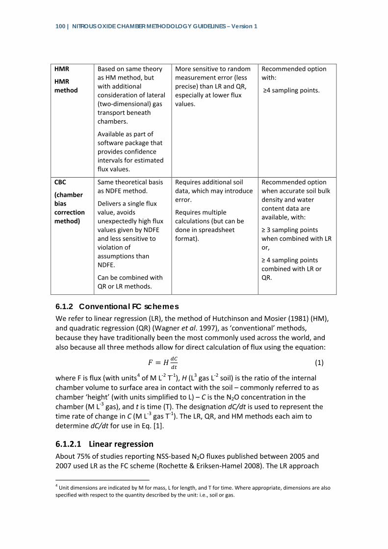
100 | NITROUS OXIDE CHAMBER METHODOLOGY GUIDELINES – Version 1
HMR
HMR method
Based on same theory as HM method, but with additional consideration of lateral (two-dimensional) gas transport beneath chambers.
Available as part of software package that provides confidence intervals for estimated flux values.
More sensitive to random measurement error (less precise) than LR and QR, especially at lower flux values.
Recommended option with:
≥4 sampling points.
CBC
(chamber bias correction method)
Same theoretical basis as NDFE method.
Delivers a single flux value, avoids unexpectedly high flux values given by NDFE and less sensitive to violation of assumptions than NDFE.
Can be combined with QR or LR methods.
Requires additional soil data, which may introduce error.
Requires multiple calculations (but can be done in spreadsheet format).
Recommended option when accurate soil bulk density and water content data are available, with:
≥ 3 sampling points when combined with LR or,
≥ 4 sampling points combined with LR or QR.
6.1.2 Conventional FC schemes We refer to linear regression (LR), the method of Hutchinson and Mosier (1981) (HM), and quadratic regression (QR) (Wagner et al. 1997), as ‘conventional’ methods, because they have traditionally been the most commonly used across the world, and also because all three methods allow for direct calculation of flux using the equation:
𝐹 = 𝐻 𝑑𝐶𝑑𝑡
(1)
where F is flux (with units4 of M L-2 T-1), H (L3 gas L-2 soil) is the ratio of the internal chamber volume to surface area in contact with the soil – commonly referred to as chamber ‘height’ (with units simplified to L) – C is the N2O concentration in the chamber (M L-3 gas), and t is time (T). The designation dC/dt is used to represent the time rate of change in C (M L-3 gas T-1). The LR, QR, and HM methods each aim to determine dC/dt for use in Eq. [1].
6.1.2.1 Linear regression About 75% of studies reporting NSS-based N2O fluxes published between 2005 and 2007 used LR as the FC scheme (Rochette & Eriksen-Hamel 2008). The LR approach
4 Unit dimensions are indicated by M for mass, L for length, and T for time. Where appropriate, dimensions are also specified with respect to the quantity described by the unit: i.e., soil or gas.
Chapter 6: Data Analysis Considerations | 101
simply uses the slope obtained from least-squares linear regression of C versus t to estimate dC/dt for use in Eq. [1]. Obviously, applying LR to inherently non-linear data, as described above, will in theory tend to underestimate F0, and this has been shown in several studies (e.g. Matthias et al. 1978). While this is universally recognised, LR is nevertheless widely used because of its practical advantages. It is computationally simple, and applicable to low numbers of chamber observations (e.g. n=2). However, while using two time points per chamber deployment may be attractive logistically, it does not allow for any evaluation of non-linearity, nor the statistical confidence of the estimate.
Some researchers have justified the use of LR and/or two sampling points, based on preliminary measurements showing a high degree of linearity in chamber data for a particular site. However, diffusion theory predicts that: (i) even relatively small deviations from linearity can result in substantially biased LR-based flux estimates; and (ii) the extent of non-linearity in chamber data can vary considerably among measurements, depending on soil physical properties (e.g. water content), which can range widely over time and space (Livingston et al. 2006; Venterea and Baker 2008).
For example, Conen and Smith (2000) used numerical modelling to show that when LR was applied to theoretical chamber data exhibiting r2 values greater than 0.997, F0 was underestimated by more than 25%, even at a relatively low value of soil air-filled porosity (i.e., 20%). Venterea and Parkin (2012) showed how increasing air-filled porosity leads – in theory – to increased non-linearity in chamber data and correspondingly increased underestimation of F0, due to increasing accumulation of gas within the soil pores instead of the chamber. Conen and Smith (2000) refer to this phenomenon as N2O “storage” within the soil profile.
Venterea and Parkin (2012) and Venterea and Baker (2008) demonstrated that such soil property effects on flux underestimation imply that LR (and potentially other FC schemes) will be more or less accurate at different times and/or in different places during a field experiment, thereby leading to biases that could confound the results. Nevertheless, compared with the QR and HM schemes, LR-based estimates are least sensitive to random variations in chamber N2O concentrations resulting from sampling techniques and performance of analytical instruments: in other words, from variations arising from ‘measurement error’ (Venterea et al. 2009). Similarly, LR has been shown to have the lowest method detection limit, compared with other schemes (Parkin et al. 2012).
In this sense, LR can be said to have greater precision compared with other schemes, while at the same time having the greatest expected bias. Furthermore, LR’s precision relative to other FC methods is expected to increase as the number of sampling points (n) collected per DP decreases (Venterea et al. 2009). This fact, combined with the lack of statistical robustness of non-linear FC methods when n < 4 (see sections below), leads us to recommend that LR be used when n = 3.
In addition, under certain circumstances, precision might be considered of equal or perhaps greater importance than bias. For example, Venterea et al. (2009) showed that LR-based flux estimates can be more statistically robust for detecting differences
102 | NITROUS OXIDE CHAMBER METHODOLOGY GUIDELINES – Version 1
in fluxes among experimental treatments, by reducing the additional variance contributed by measurement error.
The advantage of LR in this regard will depend on the magnitude of the flux in relation to measurement error, and to other factors which may be difficult to predict (Venterea et al. 2009). One option is to calculate fluxes using both LR and a non-linear scheme, then determine if means comparisons or statistical relationships using LR-based flux estimates are more robust. Of course, in this case, it must be kept in mind that the LR-based estimates will more greatly underestimate F0 than a non-linear scheme.
Another situation where LR may be the only reasonable option is when a chosen non-linear scheme ‘fails’ when applied to a particular set of chamber data. All other FC schemes essentially assume that chamber data will have decreasing slope over time. In practice, measurement error and/or other factors (e.g. temperature or pressure variations) may result in data that display near-perfect linearity or curvature that is ‘opposite’ to the expected pattern (i.e., increasing slope over time). In the latter case, non-linear FC schemes tend to produce a flux estimate less than that produced by LR, which is an unreasonable outcome.
Thus, when using methods other than LR, it is advisable to evaluate each individual data set for method ‘failure’, as discussed below. In these cases, use LR, or perhaps remove any clearly anomalous data points responsible for the method failure.
6.1.2.2 The HM method The non-linear FC scheme, first proposed by Hutchinson and Mosier (1981), is very commonly used in N2O work. However, the theoretical basis and underlying assumptions of the HM model may not be as widely understood. The assumptions are that: (i) the N2O gas concentration at some depth d in the soil is a constant (Cd) during the chamber deployment period; (ii) the physical properties (e.g., water content, bulk density) that control soil-gas diffusion are uniform in the soil layer above the depth d, and (iii) the flux of gas into the chamber is controlled by one-dimensional (1D) vertical diffusion, proportional to a linear soil-gas concentration gradient (dC/dt) between d and the soil surface.
With these assumptions, the rate of change in chamber N2O concentration (C) can be described by a simple ordinary differential equation given by:
𝑑𝐶𝑑𝑡
= 𝑘(𝐶𝑑 − 𝐶) (2)
where = 𝐷𝐻𝑑
, and D is the soil-gas diffusion coefficient (L3 gas L-1 soil T-1) in the soil
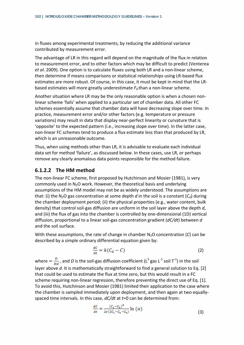
layer above d. It is mathematically straightforward to find a general solution to Eq. [2] that could be used to estimate the flux at time zero, but this would result in a FC scheme requiring non-linear regression, therefore preventing the direct use of Eq. [1]. To avoid this, Hutchinson and Mosier (1981) limited their application to the case where the chamber is sampled immediately upon deployment, and then again at two equally-spaced time intervals. In this case, dC/dt at t=0 can be determined from:
(3)
Chapter 6: Data Analysis Considerations | 103
where C0, C1, and C2 are the chamber N2O gas concentrations measured immediately after chamber deployment, after the first interval, and after the second interval, respectively, Δt is the time interval between each sample, and . In this case,
F can be calculated directly from Eqs. [1] and [3].
In addition to being restricted to the case of three equally-spaced time points, Eq. [3] will fail when α=1 (F = 0) and when α ≤ 0 (ln (α) is not defined). Also, when 0 ≤ α ≤ 1, unexpected curvature will occur as discussed above. Thus, combining these three cases, reasonable model failure criteria for the HM method would be to exclude all cases where α ≤ 1, in which cases applying LR instead may be more reasonable (Venterea et al. 2009).
The main advantage of the HM method is that it has some degree of theoretical basis: it is computationally straightforward, and allows for explicit use of Eq. [1]. On the other hand: (i) compared with LR and QR, the HM method has been shown to be most sensitive to measurement error, and therefore less precise than these other methods; (ii) HM cannot be used with > 3 sampling points, unless an averaging procedure is used – for example, by using four equally-spaced time points and using the average of the middle two time points as the second point – and (iii) HM cannot generate statistical data (e.g., confidence intervals, r2 values). For these reasons, the HM method is not recommended.
6.1.2.3 Quadratic regression The quadratic regression (QR) method proposed by Wagner et al. (1997) assumes that chamber gas concentration will change as a function of time, according to:
𝐶(𝑡) = 𝑎𝑡2 + 𝑏𝑡 + 𝑐 (4)
where a, b, and c are regression coefficients. Because the first derivative of Eq. [4] at t=0 is equal to b, the flux at time zero (F0) can be estimated by substitution of b for dC/dt in Eq. [1]. Like LR, QR is empirical, with no physical basis. The QR method can be applied without necessarily using non-linear regression; for example, the multiple regression (LINEST) function in Microsoft Excel can be applied in spreadsheets by treating t and t2 as separate independent variables.
The QR method can be used with more than three sampling points, and – in contrast to the original HM method – with any (e.g. non-uniform) sampling interval. Because Eq. [4] contains three regression coefficients, more than three sampling points are recommended when using QR. When more than three sampling points are used, the LINEST function can be used to return model statistics, including R2 and the standard error of the estimate of b. In contrast, the original HM model allows for only three equidistant sampling points; therefore model statistics cannot be determined (limitations in number and distribution of samples are overcome in the HMR model, see section 6.1.3.3).
Because Eq. [4] can be fitted to data displaying a wide range of non-linear patterns, it is recommended that model failure criteria be used when applying the QR method. Evaluation of model failure can be facilitated by using the value of the second
104 | NITROUS OXIDE CHAMBER METHODOLOGY GUIDELINES – Version 1
derivative of Eq. [4], which is equal to 2a. Unexpected data curvature will occur whenever a and b have the same sign, or in other words, whenever ab> 0. QR is more flexible in terms of sampling regime, and less sensitive to measurement error, compared with HM (Venterea et al. 2009). Theoretical analysis has indicated that QR produces more accurate flux estimates than LR, but less accurate than HM in the absence of measurement error (Livingston et al. 2006; Venterea et al. 2009).
6.1.3 Advanced FC schemes We apply the term ‘advanced’ to FC schemes which have a more rigorous or extended theoretical basis than conventional schemes, and which require additional numerical computation beyond direct calculation using Eq. [1]. Included in this category are the NDFE (Livingston et al. 2006), CBC (Venterea 2010), and the extended HM/HMR methods (Pedersen et al. 2010). Each of these schemes has its advantages and disadvantages, and currently, neither can be recommended as better overall. We do, however, recommend that when ≥ four points are sampled, a non-linear scheme be used: the recommended options therefore include LR with CBC, QR with or without CBC, NDFE alone, or HMR alone. The discussion below is provided so that users can make informed decisions about FC scheme selection.
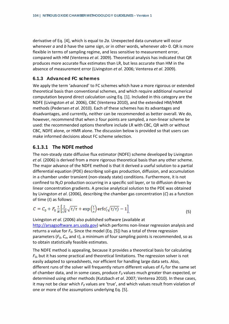
6.1.3.1 The NDFE method The non-steady state diffusive flux estimator (NDFE) scheme developed by Livingston et al. (2006) is derived from a more rigorous theoretical basis than any other scheme. The major advance of the NDFE method is that it derived a useful solution to a partial differential equation (PDE) describing soil-gas production, diffusion, and accumulation in a chamber under transient (non-steady state) conditions. Furthermore, it is not confined to N2O production occurring in a specific soil layer, or to diffusion driven by linear concentration gradients. A precise analytical solution to the PDE was obtained by Livingston et al. (2006), describing the chamber gas concentration (C) as a function of time (t) as follows:
. (5)
Livingston et al. (2006) also published software (available at http://arsagsoftware.ars.usda.gov) which performs non-linear regression analysis and returns a value for F0. Since the model (Eq. [5]) has a total of three regression parameters (F0, Co, and τ), a minimum of four sampling points is recommended, so as to obtain statistically feasible estimates.
The NDFE method is appealing, because it provides a theoretical basis for calculating F0, but it has some practical and theoretical limitations. The regression solver is not easily adapted to spreadsheets, nor efficient for handling large data sets. Also, different runs of the solver will frequently return different values of F0 for the same set of chamber data, and in some cases, produce F0 values much greater than expected, or determined using other methods (Kutzbach et al. 2007; Venterea 2010). In these cases, it may not be clear which F0 values are ‘true’, and which values result from violation of one or more of the assumptions underlying Eq. [5].
Chapter 6: Data Analysis Considerations | 105
One of these assumptions is that the soil is vertically uniform, with regard to water content and bulk density. Venterea and Baker (2008) showed that the NDFE can underestimate – and in some cases overestimate – F0 when applied to soil profiles having realistically non-uniform physical properties. Another assumption behind Eq. [5] is that chamber placement does not cause gas to diffuse horizontally beneath the chamber, which would further alter the curvature of the C versus t data. In other words, the method assumes only 1D diffusion, and therefore predicts in principle that chamber gas concentration will increase ad infinitum.
The validity of the assumption of no horizontal diffusion depends on the insertion depth of the chamber base walls into the soil, combined with the soil air-filled porosity, and the duration of chamber deployment. Hutchinson and Livingston (2001; 2002) provided criteria for determining the minimum insertion depth required to minimise this effect.
Livingston et al. (2006) numerically investigated the sensitivity of the NDFE model to chamber insertion depth, and found that the use of insertion depths less than those recommended by Hutchinson and Livingston (2001; 2002) resulted in NDFE overestimating F0. Kutzbach et al. (2007) provided some empirical support for the potential importance of horizontal diffusion effects on NDFE-based flux estimates, and its inadequacy under some circumstances, such as shallow chamber insertion depths in porous soils. The extended HM model (section 6.1.3.3) attempts to account for additional non-linear curvature due to horizontal diffusion (Pedersen et al. 2010).
6.1.3.2 The CBC method The chamber bias correction (CBC) method developed by Venterea (2010) utilises the same fundamental theory as Livingston et al. (2006), but applies it in a way that avoids non-linear regression. The CBC method is applied by first determining the flux using a conventional FC scheme (LR, HM, or QR). The initial flux estimate is then multiplied by a theoretically-based correction factor, which is calculated from soil physical properties (bulk density, water content, clay content, and temperature), chamber height (H) and total chamber deployment period (DP).
The CBC method utilises the fact that the τ term in Eq. [5] has physical meaning related to soil physical properties and H, and that the error of the initial flux estimate is
predictably related to the quantity , Venterea (2010) describes the theoretical
basis and mechanics for calculation of correction factors. An example spreadsheet is at http://www.ars.usda.gov/pandp/people/people.htm?personid=31831. Advantages of the CBC method are that it preserves the theoretical basis of the NDFE method, but overcomes some of its limitations. For example, it attempts to overcome the assumption of the NDFE method that water content and bulk density are vertically uniform by using soil physical properties averaged over the upper 10 cm of the soil profile. The CBC method avoids the need for a non-linear regression solver, and therefore delivers a single flux value, calculated using a conventional spreadsheet. It avoids generation of extraneously high flux estimates that are sometimes observed with the NDFE method (Venterea 2010; 2013).
106 | NITROUS OXIDE CHAMBER METHODOLOGY GUIDELINES – Version 1
On the other hand, the method requires additional soil property data. While these data are commonly available in many studies because of their influence over N2O production, these additional measurements necessarily introduce additional sources of potential error. The sensitivity of CBC-based flux estimates to errors in soil property measurements has been recently quantified (Venterea and Parkin, manuscript in preparation).
6.1.3.3 The extended HM model and the HMR method Pedersen et al. (2010) developed the HMR method, which builds on the original method of Hutchinson and Mosier (1981) but with expanded applicability. It has seen increasing application in some studies (e.g. Petersen et al. 2012). The HMR method is actually a comprehensive flux-calculation software available as an add-on package to be used with the R statistical programme (available at http://cran.opensourceresources.org/). The HMR method includes within it a FC scheme that expands the theoretical basis of the HM model to account for lateral (2D) gas diffusion induced by chamber placement and/or gas leaks from an imperfectly sealed chamber. This is accomplished by modifying the governing equation initially given by Eq. [2] as follows:
(6)
where the term γ(C - Co) accounts for lateral diffusion and chamber leaks. Eq. [6] can be re-arranged in the form of Eq. [2] with different values of Cd and k, but the same initial flux, which means that the flux estimate is independent of lateral diffusion and chamber leaks, as modelled by Eq. [6]. HMR can fit the HM model by non-linear regression to concentration measurements from three or more sampling time-points and arbitrary sampling intervals.
Further, HMR uses a one-parameter criterion which facilitates the search for the optimal fit: the HMR estimation procedure restricts the parameter space to ensure that estimated values are valid HM model parameters. The HM model (Eq. [2]) has the linear model (LR) and the constant model (no flux) as limiting cases (LR: k → 0; No flux: k → ∞). Therefore, when HMR detects that the criterion function is ever improving for k, approaching either zero or infinity, it recommends data to be analysed by LR, or no analysis, respectively. HMR leaves the choice of analysis to the user, and provides diagnostic plots to support a qualified decision.
For all supported analyses, HMR provides p-values 95% confidence intervals for the estimated flux, based on standard asymptotic statistical theory. The principles of the HMR estimation and classification procedure could also be applied to the NDFE model, which also has the linear and the constant model as limiting cases (LR: τ → ∞; No flux: τ → 0). As mentioned above, some studies have shown that, in practice, the NDFE model often does not fit measured chamber concentrations well, possibly due to violations of the NDFE assumption of no horizontal gas transport or other assumptions.
Analysing data with low signal-to-noise ratio is particularly challenging with non-linear FC schemes. There is always a risk that chamber concentrations by chance, even at
Chapter 6: Data Analysis Considerations | 107
sites with no flux, will follow a clear non-linear pattern, which may fool the HMR procedure to erroneously estimate a large and seemingly statistically significant flux. The variation of chamber measurements must be evaluated against the site-specific natural variation of the trace gas concentration (e.g., derived from repeated pre-deployment sampling), but this is not presently part of the HMR method.
6.1.4 Criteria for selecting FC scheme for particular applications Which is the best FC method? As described above, several criteria must be considered when selecting an analysis technique to apply to a given data set. Several studies have evaluated some of the aforementioned methods with regard to the bias (accuracy) associated with the calculated flux estimate (Livingston et al. 2006; Venterea et al. 2009; Venterea 2010; Pedersen et al. 2010; Venterea, 2013).
However, in addition to bias, the variance associated with the calculation method must also be considered. Every analytical technique for gas measurement has an associated error (see Chapter 4, section 4.4 - 4.7). In the case of gas chromatography, the precision (coefficient of variation) of the gas measurements is often in the range of 1 to 6% when small (0.2 to 1.0 ml) gas samples are used. The error associated with gas measurement (as well as other sampling errors) can result in the occurrence of ‘noisy data’ (Anthony et al. 1995), and this ‘noise’ – induced by sampling and analytical variability – can introduce a variance component to the flux estimation method. Thus, the variance of the flux estimation method should also be considered, as well as its bias.
A statistical analysis by Venterea et al. (2009) demonstrated clear trade-offs between bias and variance in selecting a flux-calculation scheme, with linear regression having greater bias, but less variance compared with the HM and Quad methods. When an estimation method has both bias and a variance component, the appropriate selection criterion is the Mean Square Error (MSE), which combines the bias and variance (Eq. 7) (DeGroot 1986):
MSE = Variance + Bias2 (7)
Parkin and Venterea (manuscript in preparation) investigated these issues further, using Monte Carlo simulation to evaluate the bias, variance, and MSE of linear regression, the HM method, and the Quad method when applied to data sets of three or four points, with chamber deployment times of 0.5 h, 0.75 h and 1.0 hour, and different degrees of data curvi-linearity. Monte Carlo simulations were performed by constructing simulated N2O chamber data, using the method described by Venterea et al. (2009). This analysis was applied over a range of analytical precisions (1% to 6%), and showed there is no simple answer to the question: “Which flux calculation method is the best?”
The MSE of a given flux calculation method is dependent upon three factors: i) the magnitude of the underlying flux; ii) the degree of data curvi-linearity and iii) the analytical precision. The reader is referred to Parkin and Venterea (2010) for preliminary results of this analysis. Additional analysis is under way (Parkin and Venterea, manuscript in preparation). It is quite possible that analysis of N2O flux
108 | NITROUS OXIDE CHAMBER METHODOLOGY GUIDELINES – Version 1
results from complex environments – where fluxes may range over several orders of magnitude and display different types and degrees of non-linear curvature – will require a combination of FC methods to obtain the best overall precision and minimum bias. The HMR software (section 6.1.3.3) enables the analyst to choose between LR and a non-linear model (or zero flux) for each individual data set, based on scatter plots. This approach could be extended by more stringent criteria to guide the decision on flux calculation method.
6.2 Estimation of cumulative emissions using non-continuous flux data
Accurately determining N2O fluxes from agricultural soils is a major challenge, due to the large spatial and temporal variability of the microbial processes that generate them, and their interaction with environmental variables. Long-term studies are recommended, as fluxes vary from year to year (Velthof and Oenema 1995): unusual weather in one year will affect subsequent emissions that year, and thereafter.
6.2.1 Accounting for spatial variability The spatial variability in N2O emissions (as discussed in Chapter 3) means that large coefficients of variation are often encountered in flux data derived from static chamber measurements: e.g., 50-100% for CH4 (Whalen and Reeburgh 1988); 13-57% (Yamulki et al. 1995) and 31-168% for N2O (Matthias et al.1978). Calculation of mean fluxes from a replicated experiment must therefore give a representative value of the spatial variability of the plot in question. This spatial variability has been considered log-normal at all scales (Oenema et al. 1997), although normal distributions have also been reported, in which case arithmetic means are used (Petersen 1999).
It has been suggested that the type of distribution can change at different times of the year (Tiedje et al. 1989). Normal distribution would be expected when the soil is wetter and more homogeneous. In the summer, when the soil is dry, hot spots are expected, producing a log-normal behaviour (Parkin 1987; Tiedje et al. 1989). A third type of distribution has been reported, in clusters, which shows two or more groups of data (see Chapter 3, section on Strategic Sampling). In this case, a mean per cluster is calculated, and these means are then averaged to give the plot mean. Cardenas et al. (2010) observed that the mean of the cluster means was biased by large values when these were a minority in the data set and noted that the bias could have been due to different numbers of data points in each cluster.
Another suggested method is the Kriging technique, in which gaps in data in a field (spatial gaps, areas of the field with no measurements) are filled in, but it relies on spatial autocorrelation between measured fluxes (Folorunso & Rolston 1984). It is however, common to have only few chambers (fewer than 10) to measure fluxes from a particular treatment at field scale, restricting the possibility of attributing the relevant distribution (Velthof & Oenema 1995). In this case, normal distribution is usually assumed and arithmetic means determined (Cardenas et al. 2010).
Chapter 6: Data Analysis Considerations | 109
6.2.2 Accounting for temporal variability As discussed in Chapter 5, the more frequently measurements are made, the more accurate the integrated seasonal/yearly cumulative flux estimate will be (Smith & Doobie 2001; Parkin 2008). When estimating daily and cumulative fluxes, certain components of temporal variability must be considered, including diurnal variations, and variations from perturbation, such as tillage, fertility, irrigation, rainfall and thawing. To account for diurnal variability, it is recommended that fluxes are measured at times of the day that more closely correspond to the daily average temperature (mid-morning, early evening). Q10 temperature correction may be used to adjust daily flux rates to the average daily temperature, but caution is warranted.
The temperature correction procedure assumes that temperature variations are the primary factor driving diurnal flux variations – an assumption that may not be universally true. Selection of both the appropriate Q10 factor and soil temperature (depth) are critical. The time lag between gas production in the soil profile, and gas flux from the soil surface, will dictate the appropriate soil temperature to use in performing the Q10 flux correction. Biological reaction rates increase exponentially with temperature between 15 – 35°C, and Q10 values found in the literature range between 1.6 for conditions conducive to nitrification (Smith et al. 1998), to 15 in heavy soils under wet conditions conducive to denitrification (Dobbie et al. 1999; Smith et al. 1998).
Temperature also affects the solubility of gases in water, as well as their rates of diffusion in the soil profile, affecting N2O as well as O2 diffusion. These in turn affect anaerobicity, suggesting a complex effect of temperature on fluxes. The appropriate Q10 factor, then, must be carefully determined when using a temperature correction.
Frequent sampling is recommended to account for temporal variation caused by perturbation, both before and after the events (Chapter 3). To calculate cumulative fluxes, the daily fluxes can then be integrated, using the trapezoidal integration method. However, this method could overestimate fluxes, especially if measurements are carried out more intensively around events (fertiliser application, rainfall) or if measurements are infrequent, especially around the time of larger fluxes.
Therefore, there may be a need to fill in the gaps when there are no measurements taken. This could be done by extrapolating the last pre-perturbation flux measurement over time, until just before the perturbation. Emissions between events (background fluxes) can also be used to calculate mean daily background fluxes, then extrapolated to the year by multiplying by the number of days not affected by events. However, this can underestimate emissions, as changes in soil mineral N (especially when organic carbon is high, or when crop residues are incorporated) could provide the N necessary for the production of N2O at those times when emissions are not expected to be great (Dobbie and Smith 2001; Webster and Goulding 2006). Empirical or process-based models can also be used to estimate fluxes on those times and locations where measurements were not carried out.
110 | NITROUS OXIDE CHAMBER METHODOLOGY GUIDELINES – Version 1
6.3 Assessment of minimum detectable flux (MDF) Past efforts to assess the minimum detection limits of soil gas emissions have focused on determining goodness-of-fit of regression procedures. For fluxes determined by linear regression, a t-test of the slope of the regression line can be used to assess if the flux is significantly different from zero (Livingston & Hutchinson 1995; Rochette et al. 2004). Since standard errors of the model parameters obtained in the Quad and HMR methods can also be calculated, a t-test of significance can be applied to determine the significance of fluxes derived by these methods.
The HM flux procedure does not allow for calculation of an associated standard error directly. However, the stochastic application of the HM procedure developed by Pedersen et al. (2001) does provide flux estimates with associated confidence limits, enabling the determination of regression significance. Typically, goodness-of-fit tests are applied at an α level of 0.05. However, in computations of trace gas fluxes with three or four data points, degrees of freedom will be small (degrees of freedom = number of time points, minus number of model parameters). When the number of degrees of freedom is small, the power to detect significance is low, thus the type II5 error rate will be high. In addition, whereas goodness-of-fit tests can determine whether a given flux is significantly different from zero, they do not provide an indication of the magnitude of the minimum detectable flux.
Using Monte Carlo sampling, Parkin et al. (2012) developed a method to determine the minimum detection limits for several different regression models when three or four data points are available. This method allows the calculation of the flux minimum detection limit if the chamber deployment time (DT) and sampling/analytical precision (coefficient of variation) are known (see Appendix 3 for an example of this calculation).
6.4 Statistical considerations for analysing inherently heterogeneous flux data
6.4.1 Assessment of normality and transformation The high variability of N2O emissions often manifests as positively skewed distributions. These in turn arise because many environmental variables cannot take on negative values, and are therefore constrained by zero. Before applying any standard analysis of variance procedures, several assumptions must be established concerning the underlying error structure of the data. Among these is the assumption of normality. The effects of violations of the assumption of normality on the efficacy of parametric statistical tests, such as the t-test, have long been known (Hey, 1938; Cochran, 1947).
Non-normality will influence the ability of a statistical test to perform at the stated a-level – an effect Cochran (1947) refers to as the validity of the test. Non-normality also affects the power of a statistical test to detect differences when real differences in the data actually exist. Two common procedures have been recommended for when data
5 Failure to reject false null hypothesis
Chapter 6: Data Analysis Considerations | 111
are not normally distributed: (i) transform for normality, or (ii) apply nonparametric statistical methods (Snedecor and Cochran 1967).
These two approaches, though, have consequences for the inference base – specifically with regard to the estimand – which are not typically considered. This discussion will focus on log-normally distributed data, and present information on (i) optimal methods for computing the mean and variance for a log-normally distributed variable, and (ii) guidelines for hypothesis testing.
6.4.2 Estimating the mean and variance of log-normally distributed data In most environmental studies, it is impossible to sample the entire population of the variable of interest. Thus, we are forced to estimate the parameters of the underlying population – such as the mean and variance – from sample data. Estimating the mean and variance for normally distributed data is straightforward. But sample data is often positively skewed, and is better approximated by the two-parameter log-normal distribution. When log-normality exists, statistical methods of analysing Gaussian data are not ideal: there are better techniques for estimating the population mean, median, and variance from sample data (Parkin and Robinson 1992; Parkin et al. 1988).
These alternatives yield unbiased parameter estimates, and have minimum variance. In addition, exact methods for computing confidence limits of the mean and median are known (Parkin et al. 1990). Three methods have typically been applied to estimate the mean and variance of log-normally distributed data. These are the method of moments (MM), the maximum likelihood method (ML) and the uniformly minimum variance unbiased estimator (UMVUE) method.
6.4.2.1 Method of Moments estimators (MM) Method of Moments (MM) estimators are computed according to the standard methods found in common statistical texts (the mean is the arithmetic average of the sample values, and the variance is the average squared deviation from the mean):
(8)
(9)
where xi = the untransformed ith observation, n = the number of observations, m = the estimate of the population mean, and s2 = the estimate of the population variance.
The MM estimators are unbiased, irrespective of the underlying distribution. However, they have higher associated variance than the UMVU estimators when applied to log-normal data, and so are less efficient.
6.4.2.2 Maximum Likelihood estimators (ML) Maximum Likelihood (ML) estimators employ the use of log-transformed sample data and compute the mean according to the asymptotic formulae shown below.
(10)
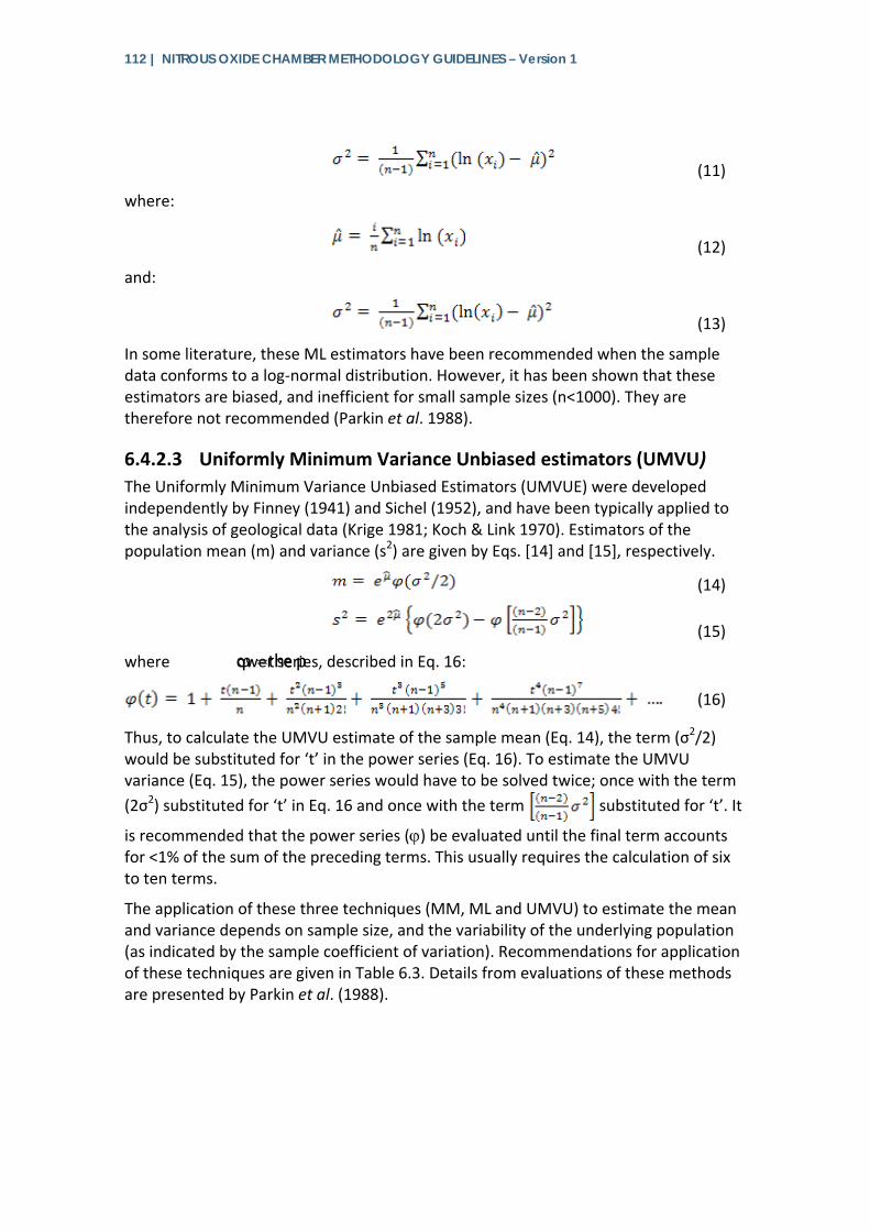
112 | NITROUS OXIDE CHAMBER METHODOLOGY GUIDELINES – Version 1
(11)
where:
(12)
and:
(13)
In some literature, these ML estimators have been recommended when the sample data conforms to a log-normal distribution. However, it has been shown that these estimators are biased, and inefficient for small sample sizes (n<1000). They are therefore not recommended (Parkin et al. 1988).
6.4.2.3 Uniformly Minimum Variance Unbiased estimators (UMVU) The Uniformly Minimum Variance Unbiased Estimators (UMVUE) were developed independently by Finney (1941) and Sichel (1952), and have been typically applied to the analysis of geological data (Krige 1981; Koch & Link 1970). Estimators of the population mean (m) and variance (s2) are given by Eqs. [14] and [15], respectively.
(14)
(15)
where ϕ = the power series, described in Eq. 16:
(16)
Thus, to calculate the UMVU estimate of the sample mean (Eq. 14), the term (σ2/2) would be substituted for ‘t’ in the power series (Eq. 16). To estimate the UMVU variance (Eq. 15), the power series would have to be solved twice; once with the term (2σ2) substituted for ‘t’ in Eq. 16 and once with the term substituted for ‘t’. It
is recommended that the power series (ϕ) be evaluated until the final term accounts for <1% of the sum of the preceding terms. This usually requires the calculation of six to ten terms.
The application of these three techniques (MM, ML and UMVU) to estimate the mean and variance depends on sample size, and the variability of the underlying population (as indicated by the sample coefficient of variation). Recommendations for application of these techniques are given in Table 6.3. Details from evaluations of these methods are presented by Parkin et al. (1988).
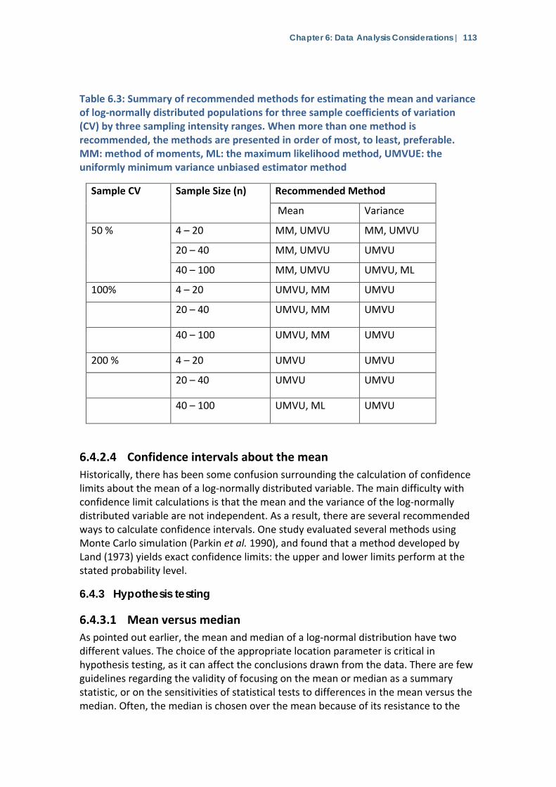
Chapter 6: Data Analysis Considerations | 113
Table 6.3: Summary of recommended methods for estimating the mean and variance of log-normally distributed populations for three sample coefficients of variation (CV) by three sampling intensity ranges. When more than one method is recommended, the methods are presented in order of most, to least, preferable. MM: method of moments, ML: the maximum likelihood method, UMVUE: the uniformly minimum variance unbiased estimator method
Sample CV Sample Size (n) Recommended Method
Mean Variance
50 % 4 – 20 MM, UMVU MM, UMVU
20 – 40 MM, UMVU UMVU
40 – 100 MM, UMVU UMVU, ML
100% 4 – 20 UMVU, MM UMVU
20 – 40 UMVU, MM UMVU
40 – 100 UMVU, MM UMVU
200 % 4 – 20 UMVU UMVU
20 – 40 UMVU UMVU
40 – 100 UMVU, ML UMVU
6.4.2.4 Confidence intervals about the mean Historically, there has been some confusion surrounding the calculation of confidence limits about the mean of a log-normally distributed variable. The main difficulty with confidence limit calculations is that the mean and the variance of the log-normally distributed variable are not independent. As a result, there are several recommended ways to calculate confidence intervals. One study evaluated several methods using Monte Carlo simulation (Parkin et al. 1990), and found that a method developed by Land (1973) yields exact confidence limits: the upper and lower limits perform at the stated probability level.
6.4.3 Hypothesis testing
6.4.3.1 Mean versus median As pointed out earlier, the mean and median of a log-normal distribution have two different values. The choice of the appropriate location parameter is critical in hypothesis testing, as it can affect the conclusions drawn from the data. There are few guidelines regarding the validity of focusing on the mean or median as a summary statistic, or on the sensitivities of statistical tests to differences in the mean versus the median. Often, the median is chosen over the mean because of its resistance to the
114 | NITROUS OXIDE CHAMBER METHODOLOGY GUIDELINES – Version 1
extreme values often observed with non-normal distributions. However, because the mean and median convey different information about the population, this rationale is not always valid.
These are the two most frequently used location parameters to summarise log-normal data. It should be recognised that the mean and median of a log-normal distribution actually convey different information about the distribution. Both of these location parameters are indicators of central tendency of the population. The mean is the centre of mass of the distribution, while the median is the centre of probability of the distribution.
In some cases, the median may be a more appropriate indicator of central tendency (Hirano et al. 1982; Loper et al. 1984; Landwehr 1978); in other situations, the mean is more appropriate (Parkin 1991; Gilbert 1987, p 45-57). The choice of the mean or the median as the summary statistic depends upon the objectives of the experiment, and the nature of the sampling. This choice between the mean and median will dictate the appropriateness of a transformation for normality, and the proper statistical test to use. A major consideration is the influence of sample volume effects on the median.
6.4.3.2 Sample volume effects on the median The central limit theorem predicts that, regardless of the form of the underlying population, the distribution of sample means approaches normality as the number of samples used in computing the means increases. An illustration of this effect is given by Parkin and Robinson (1992). In natural systems, if the variable of interest is randomly dispersed, collecting large samples has the same effect as bulking or pooling of smaller samples. Thus, for a variable that exhibits a skewed distribution, the distribution becomes more symmetrical as sample volume increases, and the value of the median increases (approaches the value of the distribution mean). This effect was observed for bacterial populations in the rhizosphere (Loper et al. 1984). The dependence of the median value on the sample volume is a major factor limiting the use of the median (and associated statistical tests of the median) as a summary parameter.
6.4.3.3 The Median as the Location Parameter of Choice When is it appropriate to use the median? A classical example illustrating a valid use of the median as a summary parameter exists in the field of economics. Personal income data are skewed, and have been approximated by a log-normal distribution. The median makes a good summary parameter for income data because the samples themselves – the individuals – have identity and significance.
The median income level allows individuals to gauge themselves against other individuals (samples) in the population. In environmental sciences, an excellent example of the appropriate use of the median is illustrated in a study of ice nucleation bacteria on plant leaves (Hirano et al. 1982). These investigators analysed 24 to 36 individual leaves, and found that the bacterial distributions on the leaves were log-normally distributed. According to the criterion statement given above, the
Chapter 6: Data Analysis Considerations | 115
appropriate use of the median requires that the samples have identity and significance.
The significance of considering the bacterial populations on the individual plant leaves is given by Hirano et al. (1982) in their statement, “The quantitative variability of epiphytic bacterial populations on individual leaves may be an expression of the uniqueness of each leaf as an ecosystem, with one or more environmental or biological characteristics significantly different from that of the neighbouring leaf.” They continue: “Since foliar plant diseases occur on individual leaves within a given plant canopy, the mean pathogen population for that canopy is of less importance than the pathogenic population on each leaf.”
For trace gas flux, the chambers can vary in size, and typically have no identity or significance. The median is not, therefore, the location parameter of choice, so normalising transformations and statistical tests on normalised data should be avoided.
6.4.3.4 The mean as the location parameter of choice Often in soil science, what is desired is an estimate of the total magnitude of a given microbial process in the ecosystem. For example, soil denitrification in agricultural systems may be an important mechanism of fertiliser N loss. Soil denitrification measurements exhibit highly skewed frequency distributions. Since the volume of a soil sample collected for denitrification determination typically has no particular significance, and because the median of a soil sample population is functionally dependent upon the volume of the samples, the median will underestimate the mass of N lost via denitrification. A possible exception may be the deliberate targeting of urine patches in grazed pastures. In this situation, if one is interested in characterising the population of urine patches, and not necessarily in estimating denitrification loss from the entire pasture, the median could be used.
The mean (centre of gravity of the distribution) is a better indicator of the total N loss from a particular system. In pollution monitoring, Gilbert (1987) defines the total mass of pollutant at a site as the ‘inventory’ of the pollutant. If the inventory of the pollutant is the desired summary variable, then the median is the wrong estimator of location, since it will systematically underestimate the total mass of material at the site (for positively skewed distributions). Since the mean should instead be the location parameter of choice, statistical tests of the mean (and not the median) should be used for hypothesis testing.
6.4.3.5 Power of hypothesis testing procedures Previous sections discussed optimum methods for computing summary statistics of log-normally distributed data. However, many studies typically wish to investigate beyond the estimation of population parameters from sample data. In many cases, sampling is conducted to evaluate treatment effects. The assumption of normality is typically required in the application of standard statistical tests. Non-normality will influence the ability of a statistical test to perform at the stated α level. Non-normality
116 | NITROUS OXIDE CHAMBER METHODOLOGY GUIDELINES – Version 1
will also affect the power of a statistical test to detect differences when real differences in the underlying populations actually exist.
The preceding discussion highlighted the fact that, with log-normally distributed variables, there is a choice of location parameters, and that the appropriate choice must be consistent with the objectives and methodologies of the problem under study. After selecting the appropriate location parameter, consideration must be given to the statistical methods used at the hypothesis testing stage. It is imperative that the experimenter who has to analyse positively skewed data understands what is being compared when log-normally transformed data, or nonparametric procedures, are used.
Parkin (1993) evaluated several hypothesis tests for determining differences in means and medians of log-normally distributed variables. He observed that transformation for normality and applying a t-test is a test of differences in medians. Such a procedure is insensitive to any differences between population means. A similar result is obtained when parametric approaches are applied. If the median is the location estimator of interest, this is not a problem. However, if the mean is the location estimator of interest, neither of these recommendations is sufficient. A t-test performed on untransformed data and the confidence limit overlap method were insensitive to differences in population median, but were sensitive to differences in population means.
At any given sample size, the t-test on untransformed data detected differences at a lower frequency than the mean confidence interval overlap method. This latter test was also operating at a Type I6 error rate substantially less than the nominal α-level at which it was applied. Thus, the mean confidence interval overlap method is a conservative test. For the log-normal case described here – regardless of whether the mean or median is the estimator of interest – at sample sizes of n = 4, very poor power is available. When lower sample numbers are available, the only way to increase power is to apply the tests at higher α levels. An Excel spreadsheet for computing the UMVU estimates of the mean and variance of a log-normally distributed variable along with Land’s exact confidence limits of the mean is available from T.B. Parkin.
6.5 Estimation of emission factor (EF) Emissions factors (EF) – representing the proportion or percentage of the N applied as urine, manure, or fertiliser emitted as N2O over the course of a growing season or annually – are often calculated from N2O emissions field data (Cardenas et al. 2010; de Klein et al. 2006). Values of the EF can be estimated by subtracting the cumulative N2O emissions occurring in a control treatment where no N was added, and from the cumulative N2O emissions in a given experimental treatment where N was added, then dividing the difference by the amount of N added. EF values can be calculated using the mean cumulative emissions for each treatment receiving N addition over all replicates, and likewise, using the mean cumulative emissions for the control
6 True null hypothesis incorrectly rejected.
Chapter 6: Data Analysis Considerations | 117
treatments over all replicates. This will obtain a single EF value for each experimental treatment, but with no indication of variance.
Alternatively, EF values can be calculated for each individual treatment replicate. In this case, cumulative emissions for the control treatment within each block (replicate) should be subtracted from the cumulative emissions for a given experimental treatment within the same block, in order to determine the EF value for that particular treatment and replicate. This procedure allows for calculation of mean and variance of each EF value, and for examining differences in the EF among treatments. In this case, users are referred to the considerations and recommendations discussed in the previous sections on statistical analysis and hypothesis testing.
It is normally expected that N2O emissions from treatments receiving added N will be greater than emissions from no-N control treatments. However, in cases where cumulative N2O emissions are greater in the control than in the treatment replicate (EF < 0), we do not recommend simply substituting EF = 0 for these values. Rather, include the actual value in the subsequent statistical analysis, unless excluding that value as an outlier is justified. It should also be noted that some studies have found non-linear relationships between amounts of N added and N2O emissions, at least for synthetic N fertiliser addition (e.g. Hoben et al. 2011). This implies that EF can vary, depending on N addition rate. Thus, it should be kept in mind that an EF calculated for a single rate of N addition may not necessarily be generalisable to other N addition rates, even within the same management and cropping system.
6.6 Conclusion Use of chambers to determine soil-to-atmosphere emissions of N2O is labor intensive and requires collection and processing of relatively large data sets. Due to the inherently variable nature of N2O emissions and the inherent tendency of chambers to alter the quantity being measured, substantial care is required to optimize analysis of the collected data. Careful consideration of appropriate analysis procedures as discussed in this chapter will ensure that upstream efforts with regard to chamber design, sampling regimes, and other aspects of the methodology will generate the most meaningful and statistically valid results.
6.7 References Anthony, WH, Hutchinson, GL & Livingston, GP, 1995, ‘Chamber measurements of soil-
atmosphere gas exchange: Linear vs. diffusion-based flux models’, Soil Science Society of America Journal, vol. 59, pp. 1308-1310.
Cardenas, LM, Thorman, R, Ashlee, N, Butler, M, Chadwick, D, Chambers, B, Cuttle, S, Donovan, N, Kingston, H, Lane, S, Dhanoa, MS & Scholefield D, 2010, ‘Quantifying annual N2O emission fluxes from grazed grassland under a range of inorganic fertiliser nitrogen inputs’, Agriculture, Ecosystems and Environment vol. 136, pp. 218-226.
Cochran, WC, 1947, ‘Some consequences when the assumptions for the analysis of variance are not satisfied’, Biometrics, vol. 3, pp. 22-38.
118 | NITROUS OXIDE CHAMBER METHODOLOGY GUIDELINES – Version 1
Conen, F, & Smith, KA, 2000, ‘An explanation of linear increases in gas concentration under closed chambers used to measure gas exchange between soil and the atmosphere’, European Journal of Soil Science, vol. 51 (no. 1), pp. 111–117.
Conrad, R, Seiler, W & Bunse, G, (1983) ‘Factors influencing the loss of fertiliser nitrogen into the atmosphere as N2O’, Journal of Geophysical Research, vol. 88, pp. 6709-6718.
DeGroot, MH, 1986. Probability and Statistics, Addison-Wesley Publishing Company, Reading, MA.
de Klein, C.A.M., Novoa, RSA, Ogle, S, Smith, KA, Rochette, P, & Wirth, TC, 2006. ‘N2O emissions from managed soils, and CO2 emission from lime and urea application’, Chapter 11 in: 2006 IPCC Guidelines for National Greenhouse Gas Inventories, Volume 4: Agriculture, Forestry and Other Land Uses, S Eggleston, L Buendia, K Miwa, T Ngara, & K Tanabe (eds.). IPCC National Greenhouse Gas Inventories Program, IGES, Japan.
Dobbie, KE, McTaggart, IP & Smith, KA, 1999, ‘Nitrous oxide emissions from intensive agricultural systems: variations between crops and seasons, key driving variables, and mean emission factors’, Journal of Geophysical Research, vol. 104, pp. 26891-26899.
Dobbie, KE & Smith, KA, 2001, ‘The effects of temperature, water-filled pore space and land use on N2O emissions from an imperfectly drained gleysol’, European Journal of Soil Science, vol. 52, pp. 667-673.
Finney, DJ, 1941, ‘On the distribution of a variate whose logarithm is normally distributed’ Journal of the Royal Statistical Society, Suppl. 7, pp. 144-161.
Folorunso, OA, & Rolston, DE, 1984, ‘Spatial variability of field-measured denitrification gas fluxes’, Soil Science Society of America Journal, vol. 48, pp. 1214–1219.
Gilbert RO, 1987, Statistical methods for environmental pollution monitoring, Van Nostrand Reinhold Co., New York.
Hey, GB, 1938, ‘A new method of experimental sampling illustrated on certain nonnormal populations’, Biometrika, vol. 30, pp. 68-80.
Hirano, SS, Nordheim, EV, Army DC & Upper CD. 1982, ‘Log-normal distribution of epiphytic bacteria populations on leaf surfaces’ Applied Environmental Microbiology, vol. 44, pp. 695-700.
Hoben, JP, Gehl, RJ, Millar, N, Grace, PR & Robertson GP, 2011, ‘Non-linear nitrous oxide (N2O) response to nitrogen fertiliser in on-farm corn crops of the us midwest’, Global Change Biology, vol. 17, pp. 1140-1152.
Hutchinson, GL & Mosier, AR, 1981, ‘Improved soil cover method for field measurement of nitrous oxide fluxes’, Soil Science Society of America Journal, vol. 45, pp. 311–316.
Hutchinson, GL, Livingston, GP, . 2001, ‘Vents and seals in nonsteady-state chambers used for measuring gas exchange between soil and the atmosphere’, European. Journal of Soil Science, vol. 52, pp.675–682.
Hutchinson, GL & Livingston, GP, 2002, ‘Soil-atmosphere gas exchange’,. pp. 1159–1182. In JH Dane & GC Topp (eds.) Methods of soil analysis. Part 4, SSSA Book Ser. 5. SSSA, Madison, WI.
Koch, GS & Link, RF, 1970, Statistical Analysis of Geological Data. Wiley, New York.
Chapter 6: Data Analysis Considerations | 119
Krige, DG, 1981. Lognormal de-Wijsian Geostatistics for Ore Evaluation, South African Institute of Mining and Metallurgy (PB1.) Johannesburg, South Africa.
Kutzbach, L, Schneider, J, Sachs, T, Giebels, M, Nykänen, H, Shurpali, NJ, Martikainen, PJ, Alm, J & Wilmking, M, 2007, ‘CO2 flux determination by closed-chamber methods can be seriously biased by inappropriate application of linear regression’. Biogeosciences Discussions, vol. 4, pp. 2279-2328.
Land, CE, 1971. ‘Confidence intervals for linear functions of the normal mean and variance’, The Annals of Mathematical Statistics, vol. 42, pp. 1187-1205.
Landwehr, JM, 1978, ‘Some properties of the geometric mean and its use in water quality standards’, Water Resources Research, vol. 14, pp. 467-473.
Levy, PE, Gray, A, Leeson, SR, Gaiawyn, J, Kelly, MPC, Cooper,MDA, Dinsmore, KJ, Jones, SK & Sheppard LJ, 2011, ‘Quantification of uncertainty in trace gas fluxes measured by the static chamber method’, European Journal of Soil Science, doi: 10.1111/j.1365-2389.2011.01403.x.
Livingston, GP, & Hutchinson GL, 1995, ‘Enclosure-based measurement of trace gas exchange: applications and sources of error’, In. PA Matson & RC Harriss (eds.) Biogenic Trace Gases: Measuring Emissions from Soil and Water. Methods in Ecology, Blackwell Science Cambridge University Press, pp. 14-51.
Livingston, GP, Hutchinson, GL & Spartalian, K, 2006, ‘Trace gas emission in chambers: A non-steady-state diffusion model’, Soil Science Society of America Journal, vol. 70, pp. 1459-1469.
Loper, JE Suslow, TV &Schroth, NM, 1984, ‘Lognormal distribution of bacterial populations in the rhizosphere’, Phytopathology vol. 74, pp. 1454-1460.
Matthias, AD, Yarger, DN & Weinback, RS, 1978, ‘A numerical evaluation of chamber methods for determining gas fluxes’, Geophysical Research Letters, vol. 5, pp. 765–768.
Oenema, O, Velthof, GL, Yamulki, S & Jarvis, SC, 1997, ‘Nitrous oxide emissions from grazed grassland’, Soil Use Management, vol. 13, pp. 288–295.
Parkin, TB, 1987, ‘Soil microsites as a source of denitrification variability’, Soil Science Society of America Journal, vol. 51, pp. 1194-1199.
Parkin, TB, 1991, ‘Characterizing the variability of soil denitrification’. In J Sorensen & NP Revsbech (eds.) Denitrification in Soil and Sediment, Plenum Publ. Corp., New York.
Parkin, TB, 1993, ‘Evaluation of statistical methods for determining differences between samples from lognormal populations’, Agronomy Journal, vol. 85 pp. 747-753.
Parkin, TB, 2008, ‘Effect of sampling frequency on estimates of cumulative nitrous oxide emissions’,Journal of Environmental Quality vol. 37, pp. 1390-1395.
Parkin, TB, Chester, ST & Robinson, JA, 1990, ‘Calculating confidence intervals for the mean of a log-normally distributed variable’, Soil Science Society of America Journal, vol. 54, pp. 321-326.
Parkin, TB, Hargreaves, SK, & Venterea, RT. 2012, ‘Calculating the detection limits of chamber-based soil greenhouse gas flux’, Journal of Environmental Quality, (accepted Jan 24, 2012).
120 | NITROUS OXIDE CHAMBER METHODOLOGY GUIDELINES – Version 1
Parkin, TB, Meisinger, JJ, Chester, ST, Starr, JL & Robinson, JA, 1988, ‘Evaluation of statistical estimation methods for log-normally distributed variables’, Soil Science Society of America Journal, vol. 52, pp. 323-329.
Parkin, TB & Robinson, JA, 1992, ‘Analysis of lognormal data’, In BA Stewart (ed.), Advances in Soil Science, vol. 20, pp. :193-235.
Parkin, TB & Robinson, JA, 1993, ‘Statistical evaluation of median estimators for log-normally distributed variables’, Soil Science Society of America Journal, vol. 57, pp. 317-323.
Parkin, TB & Venterea, RT, 2010, ‘Sampling Protocols. Chapter 3. Chamber-Based Trace Gas Flux Measurements’, In: Sampling Protocols. RF Follett (ed.), pp. 3-1 to 3-39.Available at: http://www.ars.usda.gov/SP2UserFiles/Program/212/ Chapter%203.%20GRACEnet%20Trace%20Gas%20Sampling%20Protocols.pdf(link checked 01/11/2012)
Pedersen, AR, Petersen, SO & Schelde, K, 2010, ‘A comprehensive approach to soil-atmosphere trace-gas flux estimation with static chambers’, European Journal of Soil Science, vol. 61, pp. 888-902.
Pedersen, AR, Petersen, SO, & Vinther, FP,2001, Stochastic diffusion model for estimating trace gas emissions with static chambers’, Soil Science Society of America Journal, vol. 65, pp. 49-58.
Petersen, SO, 1999. Nitrous oxide emissions from manure and inorganic fertilizers applied to spring barley. Journal of Environmental Quality, vol. 28, pp. 1610-1618.
Petersen, SO, Hoffmann, CC, Schäfer, C-M, Blicher-Mathiesen, G, Elsgaard, L, Kristensen, K, Larsen, SE, Torp, SB & Greve, MH, 2012, ‘Annual emissions of CH4 and N2O, and ecosystem respiration, from eight organic soils in Western Denmark managed by agriculture’, Biogeosciences, vol. 9, pp. 403–422.
Rochette, P, Angers, DA, Chantigny, MH, Bertrand, N & Cote, D, 2004, ‘Carbon dioxide and nitrous oxide emissions following fall and spring applications of pig slurry to an agricultural soil’,Soil Science Society of America Journal, vol. 68, pp. 1410-1420.
Rochette, P, & Eriksen-Hamel, NS, 2008, ‘Chamber measurements of soil nitrous oxide flux: Are absolute values reliable?’ Soil Science Society of America Journal, vol. 72, pp. 331–342.
Sichel, HS, 1952, ‘New methods in the statistical evaluation of mine sampling’, London Institute of Mining and Metallurgy Transactions, vol. 61, pp. 261-288.
Smith, KA, & Dobbie, KE, 2001, ‘The impact of sampling frequency and sampling times on chamber-based measurements of N2O emissions from fertilised soils’, Global Change Biology, vol. 7, pp. 933-945.
Smith, KA, Thomson, PE, Clayton, H, McTaggart, IP & Conen, F, 1998. Effects of temperature, water content and nitrogen fertilisation on emissions of nitrous oxide by soils’, Atmospheric Environment, vol. 32, pp. 3301-3309.
Snedecor, GW & Cochran, WG, 1967, Statistical methods. 6th ed., The Iowa State Univ Press, Ames, IA.
Chapter 6: Data Analysis Considerations | 121
Tiedje, JM, Simkins, S, & Groffman, PM, 1989, ‘Perspectives on measurements of denitrification in the field including recommended protocols for acetylene based methods’, Plant and soil, vol. 115, pp. 261-284.
Velthof, GL, & Oenema, O, 1995, ‘Nitrous oxide fluxes from grassland in the Netherlands 1. Statistical analysis of flux-chamber measurements’. European Journal of Soil Science, vol. 46, pp. 533–540.
Venterea, RT 2010. ‘Simplified method for quantifying theoretical underestimation of chamber-based trace gas fluxes’, Journal of Environmental Quality vol. 39, pp. 126-135.
Venterea, RT (2013). Theoretical comparison of advanced methods for calculating nitrous oxide fluxes using non-steady state chambers. Soil Sci. Soc. Am. J. Vol. 77 No. 3, p. 709-720. 10.2136/sssaj2013.01.0010.
Venterea, RT & Baker, JM, 2008, ‘Effects of soil physical nonuniformity on chamber-based gas flux estimates’, Soil Science Society of America Journal, vol. 72, pp. 1410–1417.
Venterea, RT, & Parkin, TB, 2012, ‘Quantifying biases in non-steady state chamber measurements of soil-atmosphere gas exchange’, In, Managing Agricultural Greenhouse Gases M Liebig, et al. (eds.), DOI: 10.1016/B978-0-12-386897-8.00019-X, published by Elsevier Inc.
Venterea, RT & Parkin, TB, In prep, ‘Optimizing selection of a flux-calculation scheme for determining nitrous oxide fluxes using non-steady state chambers’ (manuscript in preparation).
Venterea, RT, Spokas, KA, & Baker JM. 2009, ‘Accuracy and precision analysis of chamber-based nitrous oxide gas flux estimates, Soil Science Society of America Journal, vol. 73, pp. 1087-1093.
Wagner, SW, Reicosky, DC & Alessi, RS, 1997, ‘Regression models for calculating gas fluxes measured with a closed chamber’, Agronomy Journal, vol. 89, pp. 279–284.
Webster, CP & Goulding, KWT, 2006. ‘Influence of soil carbon content on denitrification from fallow land during autumn’, Journal of the Science of Food and Agriculture, vol. 49, pp. 131-142.
Whalen, SC, & Reeburgh, WS, 1988, A methane flux time series for tundra environments. Global Biogeochemical Cycles, vol. 2 pp. 399-409.
Yamulki, S, Goulding, KWT, Webster, CP&Harrison, RM, 1995, ‘Studies on NO and N2O fluxes from a wheat field’, Atmospheric Environment, vol. 29, pp. 1627-1635.