Embed Size (px)
Citation preview

Model Documentation
NITA s mobile LRAIC
model draft v2 cost model
17 December 2007
Our ref: 297-353
Analysys Consulting Limited
St Giles Court, 24 Castle Street
Cambridge, CB3 0AJ, UK
Tel: +44 (0)1223 460600
Fax: +44 (0)1223 460866
www.analysys.com

NITA s mobile LRAIC model
draft v2 cost
model
Model Documentation
Contents
1 General introduction 1
2 Introduction to model documentation 2
3 Installing and running the model 5
3.1 Model workbooks 5
3.2 Running the model 8
4 Main inputs 9
5 Demand and network assumptions 11
5.1 Market demand 11
5.2 Market share 13
5.3 Traffic volumes 14
5.4 Demand drivers 14
5.5 Radio network deployment 17
5.6 Transmission and switching network deployment 28
6 Network design algorithms 33
6.1 Radio network: site coverage requirement 33
6.2 Radio network: site capacity requirement (GSM and UMTS) 37
6.3 Radio network: TRX requirements 45
6.4 Backhaul transmission 46
6.5 BSC deployment 48
6.6 3G NodeB deployment 52
6.7 3G channel kit and carriers deployment 52

Model Documentation
6.8 3G backhaul deployment 53
6.9 3G RNC deployment 53
6.10 2G MSC deployment 54
6.11 Calculation of length of backbone links 59
6.12 Transit layer deployment 59
6.13 3G MSS and MGW deployment 60
6.14 Deployment of other network elements 60
7 Expenditure calculations 65
7.1 Purchasing, replacement, and capex planning periods 65
7.2 Retirement algorithm 66
7.3 Equipment unit prices 67
8 Annualisation of expenditure 70
8.1 The rationale for using economic depreciation 70
8.2 Implementation of economic depreciation principles 71
8.3 Implementation details 73
9 Service cost calculations 74
10 Glossary of abbreviations used 76
Confidential annexes (provided as separate files)
A: Draft v2 cost model for TDC
B: Draft v2 cost model for Sonofon
C: Draft v2 cost model for Telia
D: Draft v2 cost model for Hi3G
Public annexes
E: Cost of capital
F: Model updates

1 General introduction
NITA plans to finish its long-run average incremental costing (LRAIC) model for mobile
termination at the end of May 2008. At that time, NITA will make its final decision on the
LRAIC-based termination prices that will come into force from 1 January 2009.
According to the Executive order no. 1078 from 31 October 2006, NITA is obliged to use
the efficiently incurred costs of the highest-cost company as the basis for setting LRAIC
prices. As such, the LRAIC model includes the network operators TDC, Sonofon, Telia
and Hi3G.
During the process, NITA has also considered how to treat the MVNOs, Tele2 and
Barablu, in the LRAIC model. Tele2 has been acquired by Telenor, who is also the owner
of Sonofon. At this point NITA believes that Tele2 and Telenor (including and hereafter
Sonofon) should be considered as one economic entity, and NITA s decision to treat
Sonofon and Tele2 as one economic entity also applies in the context of calculating
LRAIC-based costs.
With regard to the MVNO operator, Barablu, NITA is currently as a part of its
investigation of the competition on mobile termination markets (Market 16) in the process
of performing a market analysis for Barablu. If this analysis subsequently should conclude
that Barablu has SMP and should be subject to price regulation, NITA will then consider
the configuration of this price regulation. Should it be decided to price regulate Barablu
according to the LRAIC method, this could be based on the following options:
The mobile termination rate of its host operator
The MVNO s own cost of termination plus its commercially agreed access charge
The MVNO s own cost of termination plus a calculation of the access charge on an
LRAIC basis.
It is the view of NITA, that the second and third of these approaches would be consistent
with the legislation. Because of the highest cost principle, however, the second approach
could give rise to incentives for the host operators to increase the commercially agreed
access charge. Therefore, NITA believes that the results of the third approach should be
used as a ceiling for the results from the second approach.

NITA s mobile LRAIC model
draft v2 cost model | 2
2 Introduction to model documentation
This document accompanies the draft v2 reconciled bottom-up demand, network and cost
model for long-run average incremental costing (LRAIC) distributed to Danish industry
parties on 17 December 2007.
The draft v2 bottom-up model specifies in detail the demand, network and unit cost parts of
each individual operator. A roadmap of the model is shown in Exhibit 1 below.

NITA s mobile LRAIC model
draft v2 cost model | 3
Collating market demand - voiceOperator data on historic voice usage
Collating market demand - dataOperator data on historic non-voice usage
Market scenario subs_####Historic and forecast subscribers by operator
Market scenario voice_####Historic and forecast voice traffic per sub by operator
Market scenario data_####Historic and forecast data traffic per sub by operator
Market scenario selectHistoric and forecast voice and data traffic by operator
Operator selectDemand data for selected operator
NwDes.SelectedNetwork design parameters for selected operator
NwDes.OperatorsNetwork design parameters by operator
Lifetime.InAccounting and economic asset lifetime data
Untilisation.InUtilisation inputs for operators' assets
DemCalcBusy hour demand calculations
NwDesNetwork design algorithm
FullNwOutput of network elements required by demand
NwDeployNetwork deployment schedule, retirement and purchasing algorithms
Dem.InTransposed service demand array
NwEle.OutNetwork element output (routed demand volumes)
RouFacsNetwork routing factors
CostTrendsCapex and opex unit cost trends
Unit CapexUnit capex over time
Unit OpexUnit opex over time
Costscenario.basecaseBasecase unit cost inputs
TotCapexTotal capex incurred over time
TotOpexTotal opex incurred over time
EconDepEconomic Depreciation algorithm
Com.incrCommon and incremental cost calculations
Results
Cov&Dem.InOutdoor coverage and demand calculations - normalisation of traffic by geotype
Exhibit 1: Model schematic [Source: Analysys]

NITA s mobile LRAIC model
draft v2 cost model | 4
In this draft v2 model, the demand and network aspects have been updated in response to
the operators hearing submissions and new information provided since 3 September 2007.
The costing module has been populated with a realistic set of values for costs, price trends
and the weighted average cost of capital (WACC). The bottom-up model has also been
reconciled with the top-down information submitted by each mobile operator.
This documentation covers the whole model:
Section2 introduces the model documentation
Section 3 explains how to install and run the model.
Section 4 provides a quick reference to the main inputs of the draft model.
Section 5 describes the assumptions and structure of the demand module.
Section 6 details the network design algorithms of the network module.
Section 7 describes the expenditure calculations.
Section 8 explains the cost annualisation calculations.
Section 9 details the service costing calculations
Section 10 provides a glossary of terms.
This document also provides annexes for:
Annex A: Demand and network model for TDC
Annex B: Demand and network model for Sonofon
Annex C: Demand and network model for Telia
Annex D: Demand and network model for Hi3G
Annex E: Cost of capital.

NITA s mobile LRAIC model
draft v2 cost model | 5
3 Installing and running the model
This section presents the basic operation of the model.
3.1 Model workbooks
The model is presented in an Excel workbook, called LRIC_model_NITA_draft_v2.xls,
which can be stored in a local directory and opened as a single file. There are no external
links and no macros. The model has been developed using Microsoft Excel 2000, though it
should be compatible with later versions of Excel. The structure of the Excel workbook is
detailed in Exhibit 2:
Exhibit 2: Sheet-by-sheet description of the model [Source: NITA draft demand network and
demand model, Analysys]
Sheet name Description and details of spreadsheet calculations
Input summary Summary of model inputs by operator
Roadmap Flow diagram of model calculations with hyperlinks
Con Contents description
V.H Version history
Style Style guide
Lists Definition of lists commonly used in the model
Categorisation table Operator asset, capex and opex categories
Control.Panel Selection of operator and scenarios
Collating market demand-voice
Collation and processing of voice demand for each operator
Collating market demand-data
Collation and processing of data demand for each operator
Market_scenario_ subs_static
Subscriber history and static forecast of market share
Rows 7-20: mobile penetration
Rows 23-40: market share and subscribers by operator
Rows 41-139: 2G and 3G subscribers
Rows 140-154: non-personal SIMs
Rows 156-173: GPRS subscribers.
Market_scenario_subs_evolving
Subscriber history and indicative forecast of evolution of market share
Row structure as in static subscriber sheet

NITA s mobile LRAIC model
draft v2 cost model | 6
Sheet name Description and details of spreadsheet calculations
Market_scenario_subs_converged
Subscriber history and indicative forecast of converging market share
Row structure as in static subscriber sheet
Barablu Set-up sheet for Barablu scenario
Market_scenario_subs_barablu
Subscriber history and indicative forecast of market share for Barablu
Market_ scenario_ voice_medium
Medium growth scenario for voice demand forecast (see note below)
Market_ scenario_ data_medium
Medium growth scenario for data demand forecast (see note below)
Market_ scenario_ select
Market and demand scenario subscribers and traffic for the selected market scenario
Rows 6-265: parameters from selected scenarios
Rows 266-595: calculation of volumes by service.
Operator_ select Demand parameters for the selected operator
Lifetime_In Asset lifetimes and planning periods
Cov&Dem_In Calculation of coverage area and demand per geotype
Rows 11-52: distribution of 2G demand by geotype over time
Rows 54-89: distribution of 3G demand by geotype over time.
DemCalc Conversion of service demand into cost drivers
Rows 7-56: demand volumes linked in
Rows 59-99: call duration volumes linked in
Rows 101-141: calculation of successful calls per year
Rows 143-436: calculation of busy hour load by service
Rows 439-483: input of service routeing factors
Rows 485-1113: calculation of busy hour load for each part of the network
UtilisationIn Maximum equipment utilisation, including scorched node calibration factors
NwDes.Operators Network design parameters, including spectrum allocation and asset capacities for all of the mobile operators
Rows 5-9: geotype definition
Rows 10-71: spectrum
Rows 73-100: cell radii and scorched-node outdoor coverage coefficients
Rows 102-134: blocking probabilities
Rows 137-308: area coverage
Rows 310-392: coverage and capacity deployment factors
Rows 394-512: traffic parameters
Rows 514-849: network design parameters.
Rows 851-858: 3G Licence payment sequence

NITA s mobile LRAIC model
draft v2 cost model | 7
Sheet name Description and details of spreadsheet calculations
NwDes.Selected Network design parameters, including spectrum allocation and assets capacity for the selected mobile operator
NwDes Network design calculation
Rows 6-510: 2G coverage and capacity sites
Rows 512-630: 2G transceivers
Rows 632-715: 2G backhaul
Rows 716-783: BSC layer.
Rows 786-940: 3G coverage and capacity sites
Rows 941-1017: 3G channel kit
Rows 1020-1103: 3G backhaul
Rows 1105-1145: RNC layer
Rows 1147-1253: 2G main switching layer and transmission
Rows 1256-1380: 3G main switching layer and transmission
Rows 1384-1464: other network elements.
Full_Nw Network requirements in each year
NwDeploy Purchasing and retirement algorithms expenditure schedule as a function of network requirements
Dem_In Transposes service demand
RouFac Routeing factors for network elements for average incremental cost allocation
NwEle_Out Element output routed service demand
DiscFacs WACC and discount factors for present value (PV) calculations
Costscenario.basecase
Unit capex and opex cost inputs
CostTrends Real-terms cost trends and output weighted by cost trends
UnitCapex Unit capex over time
TotCapex Total capital expenditures
UnitOpex Unit opex over time
TotOpex Total operating expenditures
EconDep Cost annualisation economic depreciation algorithm
Rows 7-158: Capex cost per unit output
Rows 162-312: Opex cost per unit output
Rows 313-465: Total cost per unit output
Rows 467-507: Fully allocated economic cost per service unit (not used elsewhere in the model)
Rows 509-670: Total economic cost recovery.
Com_incr Input of common assets by category and the incremental and common costing calculation
Rows 3-309: Total and per-unit economic costs
Rows 311-771: Input and calculation of proportion of network elements that are common

NITA s mobile LRAIC model
draft v2 cost model | 8
Sheet name Description and details of spreadsheet calculations
Rows 773-1079: Calculation of common and incremental costs by network element
Rows 1082-1426: Calculation of incremental costs per service unit and common cost mark-ups
Rows 1428-1470: Check of total cost recovery post-mark-up.
Results Marked- up costs per unit of service demand
Real.to.nominal Conversion of investment and expenditure from real into nominal terms, as required for Historic Cost Accounting (HCA) costing
HCA Cost annualisation HCA algorithm
HCA.nom.to.real Conversion of HCA result from nominal into real terms
HCA.service_cost Calculation of HCA costs per service unit
Tilted_annity Calculation of 2006 tilted annuity based costs per network element.
Erlang.table Reference table: for a given a number of TRXs or channels in a sector and a blocking probability, this table provides the capacity of the sector in Erlangs
Note: The forecast of usage per subscriber can be projected in the Market_scenario_voice_#### and Market_scenario_data_####
sheets, and selected using the model control panel. In the draft model, indicative medium growth scenarios are presented for
information only.
3.2 Running the model
In order to run the model, simply press the F9 (re-calculate) key. On some versions of
Excel, a full recalculation (CTRL + ALT + F9) may be required. The model has run and
calculated when calculate is no longer displayed in the Excel status bar. The model may
take around ten seconds to fully calculate, particularly if run on an older computer.

NITA s mobile LRAIC model
draft v2 cost model | 9
4 Main inputs
The model uses a number of input parameters, and is designed so that these can easily be
changed. The table below provides a brief description of the main inputs and their location
in the workbook.
Exhibit 3: Input parameters and their location in the model [Source: Source: NITA draft
demand network and demand model, Analysys]
Input parameter Location in the model and brief description of the input
Control panel Selection of options or scenarios to be applied to the model
Subscriber traffic forecasts
Location: Market_scenario_voice_#### and Market_scenario_data_#### worksheets
The forecast per year-average subscriber of voice and data traffic volumes per month
Market share of subscribers
Location: Market_scenario_subs_#### worksheet
The evolution of subscribers and market share from 1 January 2007.
Network roll out Location: NwDes.Operators worksheet, rows 180-308
This controls the proportion of area covered by the coverage network in each year.
Network design parameters
Location: NwDes.Operators worksheet
These parameters control all the operator specific aspects of the network design, and most of them can be modified by the user as required:
spectrum allocation
blocking probabilities
cell radii
coverage inputs
traffic assumptions (call durations, busy hour, call attempts, traffic by geotype)
maximum frequency reuse pattern
site sectorisation
site type deployment (own, third party sites)
BTS capacity
repeater/tunnel deployments
backhaul: split between microwave and leased lines
BSC capacities and remote percentage
RNC capacities and remote percentage
BSC-MSC link capacity

NITA s mobile LRAIC model
draft v2 cost model | 10
Input parameter Location in the model and brief description of the input
MSC capacities
proportions of traffic traversing the backbone network
HLR, SMSC, PCU and GSN capacities and minimum deployments.
Asset lifetimes Location: Lifetime_in
Input of asset lifetimes, planning and retirement periods.
Demand driver parameters
Location: DemCalc
This sheet contains further inputs which are require to convert demand volumes into network drivers:
SMS channel parameters
GPRS traffic parameters
UMTS channel parameters
Subscriber and PDP context registration in GSNs
Routeing factors for Radio and Transmission parts of the network
MSC processor, SMSC and GSN loading parameters.
Equipment costs Location: UnitCapex and UnitOpex
Capital and operating cost per unit of equipment, expressed in real 2006 DKK.
Equipment price trends
Location: CostTrends
Annual real-terms price trend for capital and operating cost components.
Cost of capital Location: DiscFacs
Real, pre-tax WACC and inflation.

NITA s mobile LRAIC model
draft v2 cost model | 11
5 Demand and network assumptions
5.1 Market demand
Market demand is modelled for each mobile operator for historical years, based on data
provided by NITA s statistics and information provided by the mobile operators in
response to the data request. For future years, a forecast for market subscribers and traffic
is presented.
Subscribers
The number of active subscribers in the market is calculated, with a projection of future
population and assumed level of penetration of digital mobile services. The penetration is
assumed to reach 120% by the end of the period, following a saturation formula (see
Exhibit 4).
0%
20%
40%
60%
80%
100%
120%
140%
1992
1994
1996
1998
2000
2002
2004
2006
2008
2010
2012
2014
Act
ive
SIM
s in
mar
ket
Exhibit 4:
Modelled mobile
penetration, in
terms of active
SIMs [Source:
Analysys]

NITA s mobile LRAIC model
draft v2 cost model | 12
Traffic
Information on historical traffic levels, up to 2006, is sourced from operator data. The
forecast traffic demand for each mobile operator is determined by a projection of traffic per
subscriber, multiplied by projected subscriber numbers. Traffic per subscriber is projected
for each operator using simple annual growth rates, specified in the traffic scenario sheet (Sheet Market_scenario_voice_medium, Rows 6, 14, 22 etc). The following 2G and 3G traffic services have been
modelled, split according to the information supplied by each operator:
2G and 3G Voice (incoming, outgoing off-net and on-net).
2G and 3G SMS (incoming, outgoing off-net and on-net).
2G PS data traffic.
3G PS data traffic (Release 99).
2G and 3G Incoming to VMS deposit.
2G and 3G On-net to VMS deposit.
2G and 3G On-net to VMS retrieval.
2G and 3G Technical SMS.
3G Video minutes (split by incoming, outgoing off-net and on-net).
ON 2G NR incoming, outgoing (applicable to TDC and Sonofon).
OFF 2G NR incoming, outgoing (applicable to Telia and MVNOs).
ON 3G NR incoming, outgoing (applicable to Sonofon).
OFF 3G NR incoming, outgoing (applicable to Hi3G and MVNOs).
OFF 2G MVNO SMS outgoing (applicable to MVNOs).
OFF 3G MVNO SMS outgoing (applicable to MVNOs).
The table below indicates how the various services interact with the network:

NITA s mobile LRAIC model
draft v2 cost model | 13
Radio Transmission Switch
processing
Service TRX or
CK
BSC or
RNC to
core
Inter-
connect
Inter-
switch
to VMS MSC SMSC SGSN
and
GGSN
HLR
Voice traffic
SMS traffic (1)
Voice to/from VMS (2)
Packet switched traffic (3)
Video traffic
Subscriber numbers
NR on network
NR off network (4)
Notes: (1): SMS traffic is assumed to be carried in signalling channel reservation
(2): calls which are deposited on the voicemail system do not utilise the radio network for call conveyance, although an
allocation for ringing time is included
(3): 2G PS traffic is assumed to be carried in data channel reservation; 3G packet switched data is added to the voice
Erlang load
(4): NR off the network is counted as NR on network for the corresponding other operator
Exhibit 5: Indicative interactions between network elements [Source: Analysys]
5.2 Market share
The market share of each operator can be projected in the Market_scenario_subs_####
sheets, and then selected as the subscriber scenario using the model control panel. In the
draft model, scenarios are presented for information only, rather than the definitive basis on
which costs will be calculated.
The draft model presents a slow evolution to equality of market share between the four
network operators in the long term (according to the introduction, Tele2 is expected to be
included with Sonofon for this purpose), which has been forecast using simple straight-line
trends.

NITA s mobile LRAIC model
draft v2 cost model | 14
0%
10%
20%
30%
40%
50%
60%
70%
1992
1995
1998
2001
2004
2007
2010
2013
2016
2019
2022
2025
2028
2031
2034
2037
2040
Mar
ket s
hare
of s
ubsc
riber
s
TDC Sonofon Telia Hi3G Tele2
Exhibit 6: Market shares in a slow evolution scenario [Source: Analysys]
5.3 Traffic volumes
The forecast of usage per subscriber can be projected in the Market_scenario_voice_####
and Market_scenario_data_#### sheets, and selected using the model control panel. In the
draft model, indicative medium growth scenarios are presented for information only.
5.4 Demand drivers
The total service volumes for the selected operator are converted into the main demand
drivers which are used to dimension the various network elements.
Voice services
The number of voice minutes is converted into a year-average busy-hour Erlang (BHE)
load (Sheet DemCalc, Rows 143-190) using the following inputs:

NITA s mobile LRAIC model
draft v2 cost model | 15
Proportion of annual traffic during 250 normal weekdays.
Proportion of weekday traffic occurring in the normal busy hour.
The number of voice BHE is converted into a further measure, the number of busy hour
call attempts (BHCA) (Sheet DemCalc, Rows 192-274) using inputs of:
Average call duration.
Number of call attempts per successful call (e.g. due to unanswered calls).
60d
wd
B
PPficannualtrafBHE
Where Pd = Proportion of daily traffic in the busy hour
Pw = Proportion of annual traffic in the busy week days
Bd = Number of busy (week) days
aveD
CBHEBHCA
Where C = call attempts per successful call
Dave = average duration of a successful call.
Ringing time
Voice services explicitly include the additional Erlang load presented by the ringing time
associated with calling. Ringing time occurs for calls to a B-subscriber where there is
network occupancy until the call is answered, diverted or not answered. An estimated
ringing time of 10 seconds for calls to an end user, and 5 seconds for calls to/from the
VMS, is applied to the various call types. An estimate of 5 seconds is applied to VMS calls
because some diversions are a result of a mobile ringing but not being answered, and some
diversions are immediate.
For each service, the model calculates:

NITA s mobile LRAIC model
draft v2 cost model | 16
This ringing time per minute is added to the per-minute routeing factors for radio and
transmission elements in the DemCalc routeing factor table.
SMS services
The volume of SMS messages carried in the year is converted into a messages-per-busy-
hour rate using similar inputs as the voice calculation. A throughput in messages per
second is also calculated
this is equal to messages per hour divided by 3600. A
conversion factor between SMS messages and equivalent voice minutes is also calculated,
using estimates of the average SMS length (40 bytes) and the channel rate that SMS is
carried by (assumed to be 8 SDCCH per TCH) (Sheet DemCalc, Rows 276-312).
Packet data services
Demand for data services is converted into a Mbit/s demand driver and an equivalent voice
Erlang load using assumptions of:
The proportion of traffic occurring in the downlink vs. uplink direction.
The amount of additional IP overheads to user data that is required.
The channel rate at which the data is carried (13.4kbit/s CS2 for GPRS and 16kbit/s for
UMTS).
The model also calculates the number of connected and active packet data users (to
dimension the SGSN and GGSN network elements which service the packet data demand)
using estimates of the proportions of GPRS and UMTS subscriptions which are
active/connected (Sheet DemCalc, Rows 314-351).
lDurationcessfulCalAverageSuc
ssfulCalltsPerSucceCallAttempeRingingTimeveyedMinututesPerConRingingMin

NITA s mobile LRAIC model
draft v2 cost model | 17
Video services
A relatively small volume of video traffic is included in the model. This is converted into
BHE and BHCA in exactly the same way as voice traffic, although the model assumes that
4 channels are required per Erlang when video is included in the dimensioning of radio
network elements (Sheet DemCalc, Rows 333-337).
Routeing factors
An input table of routeing factors determines the factor applied to each service volume
when calculating the load on the various parts of the network (Sheet DemCalc, Rows 439-482, 485-1113).
5.5 Radio network deployment
The main assumptions and choices about network design are documented below.
Geotypes
The model considers four geotypes: dense urban, urban, suburban and rural. These
geotypes have been defined using the data submitted by the mobile operators. The rural
geotype can be matched closely to the various rural geotypes defined by the operators
(e.g. open, woodland, etc.). However, the definitions of non-rural areas differed between
the operators. As a result, operator-specific assumptions have been made when
transforming information such as traffic proportions from the operator-defined geotypes
into the modelled non-rural geotypes.
The proportion of area within each of the defined geotypes is shown below in Exhibit 7:

NITA s mobile LRAIC model
draft v2 cost model | 18
Geotype Proportion of area Cumulative proportion
Dense urban 0.08% 0.08%
Urban 0.83% 0.91%
Suburban 3.34% 4.25%
Rural 95.75% 100%
Exhibit 7: Split of
area between
geotypes [Source:
Analysys]
In order to better understand the distribution of the geotypes across Denmark, a MapInfo
dataset of Danish postcode areas has been used to assign each postcode to a geotype. This
was done by sorting postcode areas in descending order by population density and
allocating them to geotypes based on the cumulative proportion of area in the sorted list.
The geotypes are distributed across Denmark as shown in Exhibit 8.
Dense urban
Urban
Suburban
Rural
Dense urban
Urban
Suburban
Rural
Exhibit 8:
Denmark geotypes
by postcode areas
for the purpose of
the LRAIC model
[Source: Analysys]
Each operator has supplied data for traffic split by geotype, with is used to populate the
relevant traffic distribution percentage input in the model.

NITA s mobile LRAIC model
draft v2 cost model | 19
The definition of the geotypes can be found on the NwDes_operators worksheet (for
geographical parameters) and Cov&Dem_In (for traffic distribution calculations).
Coverage
The outdoor coverage networks for each technology (primary GSM, secondary GSM and
UMTS) are calculated separately within the model. Any in-building coverage area
provided by this deployment (where the signal strength is high enough to penetrate
buildings) will be commensurately lower, though not used to drive network deployment or
traffic calculations in the model.
In order to inform this outdoor coverage profile, NITA s mast database was used. This
database provides information about the number of active GSM/UMTS BTSs installed in
the radio networks of each operator over time. It includes information on:
Technology of the BTS (GSM900, GSM1800, or UMTS).
Location of the BTS, specified in Danish co-ordinates.
Activation date of the site that houses the BTS.
The location coordinates allow each BTS to be assigned to a geotype. At any one time, the
database can only provide a snapshot of the deployment at the time: it cannot be used to
accurately build up a time series, since the activation dates refer to the site, rather than the
BTS on that site. The two dates will only coincide when a BTS is deployed on a new site.
BTSs using more recent technologies are often deployed on existing sites, so their
associated dates in the database will be earlier than the actual date of installation of the
BTS. For example, 2G/3G operators have many UMTS BTSs with dates in the database
preceding 2000, since they were deployed on sites originally built for GSM and/or NMT.
The limitations in the database for each operator and technology are displayed below in
Exhibit 9.

NITA s mobile LRAIC model
draft v2 cost model | 20
Operator GSM900 GSM1800 UMTS
TDC Limitations: overlays of all three technologies on NMT sites, UMTS overlays on GSM sites, GSM1800 overlays on GSM900 sites
Sonofon Can assume no limitations: primary spectrum
Limitations: secondary spectrum many overlays
on pre-existing sites
Limitations: UMTS overlays on GSM sites
Telia Limitations: secondary spectrum many overlays
on pre-existing sites
Can assume no limitations: primary spectrum
Limitations: UMTS overlays on GSM sites
Hi3G n/a n/a Can assume no limitations: primary spectrum
Exhibit 9: Limitations of the mast database in calculating BTS deployments over time
[Source: Analysys]
NITA was able to provide several versions of the mast database, providing snapshots at
various points in the years 2004 07. Consistency checks were carried out on these data
sets, and a number of additions and removals of data were made where appropriate, to
ensure that
Forecasted (but not yet built) BTSs were removed.
BTSs with severe information gaps (such as technology and location) were removed if
the missing information could not be provided using other versions of the database.
BTSs in earlier versions of the data persisted through to the later versions in a
consistent way (sometimes BTSs would appear in the data intermittently).
After establishing a reasonable level of consistency, a detailed treatment of the BTS
deployments for the period 2003 06 was undertaken. Specifically, the number of BTSs
was calculated for the mid-year and year-end, broken down by operator, technology and
geotype. For the cases where no limitations in the data sets can be assumed (as described in
Exhibit 9), an understanding of deployments back to 1992 has also been possible. For the
remaining cases, using the date point in the database would result in an over-estimation of
the number of BTSs over time.
Some operators provided additional databases of their BTSs, which have allowed better
historical understanding of their BTS deployments over time. The mast database
information was combined with operator-supplied data in order to define the BTS locations
NITA s mobile LRAIC model
draft v2 cost model | 21
by geotype over time. This was in turn combined with cell radii estimates to calculate the
coverage profiles over time for each operator. These profiles were checked against
operator-supplied coverage estimates.
The databases also contained partial information on site identification, allowing BTSs to be
grouped together by their site. Where this information was unavailable, the co-ordinates of
the BTS was used to ascertain whether the BTS was an overlay or not. Two or more BTSs
(from the same operator) are assumed to be co-sited if their coordinates are within 15m of
each other. This buffer zone is used to account for
Small discrepancies in the BTS location data across the various databases.
The fact that BTSs may be listed with slightly different locations, given that they are
likely to be separately positioned on the site.
For the period covered by the databases (2003 06), the number of sites by operator,
technology and geotype has been calculated for the following categories:
GSM900 only.
GSM1800 only.
GSM900 shared with GSM1800.
UMTS only.
UMTS shared with GSM900.
UMTS shared with GSM1800.
UMTS shared with both GSM900 and GSM1800.
The definition of outdoor coverage by geotype can be found on the NwDes_operators
worksheet for each spectrum band. The same sheet also contains the definition of cell radii,
as described below.
Cell radii
Two different types of cell radii are used within the model: theoretical cell radii and
effective cell radii. Effective radii are derived from theoretical radii using the process
described below.

NITA s mobile LRAIC model
draft v2 cost model | 22
Theoretical cell radii
These radii apply to the hexagonal coverage area that it is estimated a BTS of a particular type,
considered in isolation, would have. Operators were able to provide some information on the
values that these cell radii would take. The model uses a set of theoretical cell radii values
which vary by geotype and technology, but not by operator
this is because theoretical cell
radii differences are considered to be due to differences in radio frequency and geotype
(clutter). These were derived by an iterative process, shown below in Exhibit 10.
Cell radii data from operators
BTS locations by operator
Area coverage data from operators (operator, time)
Cell radii estimations (technology, geotype)
BTS locations (operator, time)
Area coverage (operator, time)
Calibrated cell radii (technology, geotype)
comparison
refin
emen
t
Area coverage (operator, geotype, technology, time)
Geotype areas
Exhibit 10:
Process for
calibrating the cell
radii and deriving
area coverage over
time [Source:
Analysys]
Each operator was able to provide several values for its total geographic coverage for a
particular technology at a particular point in time. Using the databases described above, the
location of all BTSs for that particular network at that point in time was identified.
In order to derive the total geographic coverage of the network, MapInfo was used to
construct hexagonal zones of the relevant cell radius (depending on the technology of the
BTS and the geotype that it was located in) around each BTS in the network at that time.
These hexagonal zones were then grouped together and the total area of this shape was

NITA s mobile LRAIC model
draft v2 cost model | 23
calculated using MapInfo. Importantly, areas of overlap between hexagonal cells were only
counted once. An example of such a coverage map is given below in Exhibit 11, with areas
of network coverage shown in red.
Exhibit 11:
Example of a
network coverage
map generated by
MapInfo for a single
network at a
particular point in
time [Source:
Analysys]
This process was repeated until a set of cell radii were found that gave the closest values
for geographic coverage compared with the data provided by the mobile operators.
MapInfo was then used again as the central calculation engine to derive the geographic
coverage of each network by geotype and over time.
Effective cell radii
When calculating the number of BTSs required, the LRAIC model does not know the exact
location of each BTS across the geotypes. Assuming that BTSs have hexagonal coverage
areas means that they can in theory tessellate perfectly (fit together with no overlaps).
However, in reality some BTSs are not located optimally with the result that there may be
considerable overlap between their individual coverage areas. This concept is demonstrated
below in Exhibit 12.

NITA s mobile LRAIC model
draft v2 cost model | 24
Optimal locations of BTS Sub-optimal locations of BTS occurring in reality
Optimal locations of BTS Sub-optimal locations of BTS occurring in reality
Exhibit 12:
Illustration of
optimal versus sub-
optimal BTS
locations [Source:
Analysys]
The reasons for being unable to locate BTS optimally include:
obstructions (woodland, rivers, buildings),
a lack of permissible sites to house BTSs in the vicinity, and
the site already being occupied by another operator.
As a result, once a network has reached coverage in a certain geotype, the cell radii derived
using the method described above will be larger than they would be in a real-world
network. This can be seen in Exhibit 12, since sites that are sub-optimally located (on the
right of the diagram) have less total coverage than would be assumed by a more simplistic
model (on the left).
In order to explicitly account for this overlapping effect, the model weights the theoretical
cell radii by a percentage factor to give effective cell radii. In other words, the model
assumes a sub-optimal but realistic placing of BTSs. The factor that is applied is a
consequence of the scorched-node methodology used in the model, and is therefore
referred to as a scorched-node outdoor coverage coefficient (SNOCC). The value of this
coefficient can vary by operator, technology and geotype, but is always less than 1.
Effective coverage per site = SNOCC Theoretical coverage per site
2.6
Re2 = SNOCC 2.6
Rt2

NITA s mobile LRAIC model
draft v2 cost model | 25
Where 2.6 is the
for a hexagon, Re = effective hexagonal radius, and Rt = theoretical
hexagonal radius.
The variation of this factor by operator is particularly important, since earlier market
entrants usually get first choice of the sites, and later entrants often have to use site
locations that are less optimal for their network (e.g. because it is at a different frequency).
Operators may also choose the degree to which they fill-in any gaps in outdoor coverage
and achieve a more contiguous coverage network. Variation by geotype is also of
relevance, since the effect of sub-optimality can be expected to be greater in more urban
areas, where
BTSs need to be more concentrated due to the smaller cell radii,
the higher density of buildings can create greater obstructions,
support structures (buildings, chimneys and rooftops) cannot be moved, and
the demand for sites is higher.
In order to estimate values for the scorched-node coverage coefficient, the model uses the
calculations shown in Exhibit 13.

NITA s mobile LRAIC model
draft v2 cost model | 26
Theoretical cell radii (geotype, technology)
Geographic coverage (operator, geotype, technology, time)
Geographic coverage in year of interest
(operator, geotype, technology)
Effective cell radii(operator, geotype,
technology)
Ratio of effective radius to theoretical
radius (operator, geotype, technology)
Year of interest (operator, geotype,
technology)
BTS locations (operator, geotype, technology, time)
Number of BTSs(operator, geotype, technology, time)
Exhibit 13:
Derivation of
scorched-node
coverage
coefficient [Source:
Analysys]
In order to calculate the effective cell radii, the principles that have been used are that:
a geotype can only be covered by a BTS lying within that geotype,
the year of interest is determined on the basis that if a network has
achieved full coverage of a geotype: then the year of interest is taken to be the
earliest year in which coverage is achieved,
not achieved full coverage of a geotype, but has reached a steady maximal value:
then the year of interest is taken to be the first year where that value is reached.
This situation could occur because an operator may not fully deploy to a geotype
with a particular frequency (especially secondary spectrum),
neither achieved full coverage of a geotype nor reached a steady maximal value:
then the latest year (2006) is used.
Special sites
The model considers two types of special sites: indoor sites and tunnel repeaters. Data on
these site numbers has been supplied by each operator, and they are modelled on a logical

NITA s mobile LRAIC model
draft v2 cost model | 27
deployment basis. A small proportion of total traffic is assumed to be carried by these sites.
These roll-outs are defined in the NwDes.Operators worksheet.
Sectorisation and overlay of sites with secondary GSM spectrum
Mobile operators in Denmark are subject to coverage requirements for both the
GSM900MHz and DCS1800MHz spectrum. However, when determining site numbers, the
secondary spectrum may be overlaid upon the primary spectrum site. The proportion of
secondary spectrum BTSs which are overlaid upon primary spectrum sites is calculated
from operator information in the mast database (see the Coverage subsection above).
Macro site types
Operators utilise a mix of owned and third-party sites for deploying macro site BTSs and
NodeB equipment. Data from the operators indicates that these can be broadly grouped into
the following categories:
Owned tower sites.
Owned monopole sites.
Third-party tower sites.
Third-party roof-top or other sites.
The model considers the proportion of these four types of site deployment in order to
capture the different costs associated with site acquisition, civil works and ancillary
equipment. These site types are shown in Exhibit 14.
Own tower site Third party tower site Third party roof-top site
(blue shading denotes own equipment; grey shading denotes third-party assets)
Own monopole siteOwn tower site Third party tower site Third party roof-top site
(blue shading denotes own equipment; grey shading denotes third-party assets)
Own monopole site
Exhibit 14:
Site types [Source:
Analysys]

NITA s mobile LRAIC model
draft v2 cost model | 28
The proportions of sites falling into these different categories can be found in the
NwDes.Operators worksheet.
5.6 Transmission and switching network deployment
2G and 3G backhaul configuration
The backhaul configuration is modelled on the basis of the percentage of sites in each
geotype which use microwave backhaul (8Mbit/s links which can be filled with up to four
2Mbit/s E1s) or leased-line backhaul (2Mbit/s E1 links). This backhaul configuration is
shown in Exhibit 15:
9 x E1
BSC
8Mbit/s microwave (n E1 part
filled)
AN
Indoor/Tunnel sites
n E1 leased lines per site on average
E1
E1 E1
Up to 9 BTS per AN
Fibre backbone
1 x E1
9 x E1
BSC
8Mbit/s microwave (n E1 part
filled)
AN
Indoor/Tunnel sites
n E1 leased lines per site on average
E1
E1E1 E1E1
Up to 9 BTS per AN
Fibre backbone
1 x E1
Exhibit 15:
Backhaul
configuration
(AN = access node)
[Source: Analysys]
In addition to the last mile transmission to sites by microwave or leased links, a
proportion of sites are connected to access points on the operator s national transmission
network. The proportion of sites that are also connected by an access node is estimated
from operator data, and assumed to occur primarily in rural areas (where sites may be
approximately 20km away from the nearest BSC or RNC). Access nodes are dimensioned
according to a ratio of 9 BTS per node.

NITA s mobile LRAIC model
draft v2 cost model | 29
These assumptions can be found on the NwDes_operators worksheet.
In order to capture the specifics of the Danish networks, a series of fibre transmission rings
are modelled across the three main parts of Denmark (Zealand, Funen and Jutland). These
fibre rings, illustrated in Exhibit 16 below, carry:
Backhaul traffic from the access nodes to the BSC/RNC
traffic from remotely sited BSC/RNCs to the main switching sites (MSC/MGW)
inter-switch traffic between the main switching sites.
Jutland fibre ring
Fyn fibre ring
Sjaelland fibre ring
Jutland fibre ring
Fyn fibre ring
Sealand fibre ring
Exhibit 16:
Diagram of fibre
ring deployment in
Denmark [Source:
Analysys] The red
rings indicate the
location of the fibre
rings
BSC deployment
The number of BSCs is driven by the number of transceivers (TRXs) in the network, using
a BSC capacity as supplied by each operator. The inputs associated with this deployment
can be found in the NwDes.Operators worksheet.

NITA s mobile LRAIC model
draft v2 cost model | 30
Remote BSCs and associated BSC MSC links
The model includes a certain proportion of BSCs that are deployed remotely from an MSC.
This proportion is based on operator data. The traffic transiting through these BSCs is
backhauled to the MSC using E1 links provisioned over the fibre network.
RNC deployment
The number of RNCs is driven by the number of NodeBs or the total traffic which is
handled by the network. The model is based upon data for RNC capacity as supplied by
each operator, in terms of number of NodeBs and traffic capacity. The inputs associated
with this deployment can be found in the NwDes.Operators worksheet.
MSC/VLR deployment
2G MSCs are dimensioned on the basis of the processing load handled. This load is
assessed based on the number of calls, SMSs and location updates of each type that need to
be switched. This determines the number of MSC CPUs required. See Section 6.10 for
further details.
A reference table based on the Danish mobile network structures is used to determine the
number of main switching sites (MSC locations) and TSCs based on the number of MSCs
deployed in a particular operator s network. The number of MSC locations determines the
number of logical and physical links required in the network for inter-switch transmission.
Transmission requirements determine the number of E1 port cards required to support
transmission to and from the MSCs. Four types of MSC ports are calculated, based on the
associated busy hour Erlang loads carried on the respective parts of the network:
BSC-facing ports.
Interconnection ports.
Inter-switch ports.
Voicemail server ports.

NITA s mobile LRAIC model
draft v2 cost model | 31
3G MSCs are modelled as two units
an MSC Server (MSS), and a Media Gateway
Switch (MGW). The MSS is dimensioned on the basis of the processing load handled, and
this is assessed based on the number of calls, SMSs and location updates of each type that
need to be switched. The MGW is dimensioned on the basis of port demand, which is
calculated using a similar methodology to the calculation of 2G MSC port numbers. See
Section 6.10 for further details.
Transit layer
The number of required transit switches (TSCs) is calculated on the basis of the MSC
reference table. Transit switches are assumed to be required (efficient) once the diversity of
the switching network reaches the point that fully-meshing ten MSCs across six MSC sites
becomes overly complicated. See Section 6.10 for further details.
Backbone network
As discussed in the subsection on 2G and 3G backhaul, a configuration of three fibre
backbone rings is modelled. These rings are dimensioned according to the inter-switch
traffic plus the additional traffic associated with the radio sites and remote BSC/MSCs that
are connected directly to the fibre ring.
The backbone links are assumed to be deployed in STM-1 increments, based on the
number of E1 subunits required by the various transmission types. The length of the rings
is estimated on the basis of the Danish geography.
Other network elements
Also included is an explicit calculation of the remaining significant network element
deployments: HLR, network management systems, various IN servers, billing system,
VMS, GPRS and SMS infrastructure.

NITA s mobile LRAIC model
draft v2 cost model | 32
Non-network elements
The model has been populated with elements representing the major non-network activities
of wholesale support services, business overhead services and licence fees.
NITA s mobile LRAIC model
draft v2 cost model | 33
6 Network design algorithms
This section details the algorithms used to build up the network.
6.1 Radio network: site coverage requirement
The coverage networks for each technology (primary GSM, secondary GSM and UMTS)
are calculated separately within the model.
GSM
In Denmark, both 900MHz and 1800MHz spectrum are used for coverage purposes by the
GSM operators (TDC, Sonofon and Telia). To satisfy the coverage requirements, the
number of macro sites deployed has to be able to provide coverage for a certain area
defined for each geotype, which has been calculated for the period 1992 2006 using the
data provided by the mobile operators.
The inputs to the coverage site calculations, based on the chosen GSM operator, are as
follows:
Primary and secondary spectrum,
total area covered by the mobile operator by technology, geotype and time,
cell radii for coverage, by geotype and technology,
scorched node coefficients by geotype and technology, to convert between theoretical
and effective cell radii, and
proportion of primary spectrum sites available for overlay, by geotype.
The model allows for additional future coverage to be modelled. Exhibit 17 below outlines
the model algorithm for the calculation of GSM macro sites deployed.

NITA s mobile LRAIC model
draft v2 cost model | 34
Tunnel sites (t)
Indoor sites (t)
Land area km2 (G)% area to be covered by primary spectrum
(G, t)
Coverage area km2
(G, t)
Primary spectrum effective coverage
cell radius (G)
Coverage BTS area km2 (G)
Hexagonal factorNumber of primary
BTS for coverage (G, t)
% of secondary spectrum BTS deployed
on primary site (G)
Number of primary sites for coverage (G,
t)
Land area km2 (G)% area to be covered
by secondary spectrum (G, t)
Coverage area km2
(G, t)
Coverage BTS area km2 (G)
Hexagonal factorNumber of secondary BTS for coverage (G,
t)
Number of primary sites available for
overlay (G, t)
Number of separate secondary sites required (G, t)
Total coverage sites
(G, t)
Number of secondary sectors for coverage
(G, t)Sectors per BTS (G)
Sectors per BTS (G)
Number of primary sectors for coverage
(G, t)
Scorched-node outdoor coverage
coefficient (G)
Primary spectrum coverage cell radius
(G)
Secondary spectrum effective coverage
cell radius (G)
Scorched-node outdoor coverage
coefficient (G)
Secondary spectrum coverage cell radius
(G)
(G) = by geotype. (t) = by time
Exhibit 17: GSM coverage algorithm for the selected operator [Source: Analysys]
NITA s mobile LRAIC model
draft v2 cost model | 35
The coverage sites for the primary spectrum are calculated first (Sheet NwDes, Rows 9-37). The area
covered by a BTS in a particular geotype is calculated using the effective BTS radius. The
total area covered in the geotype is divided by this BTS area to determine the number of
primary coverage BTSs required (and therefore sites) (Sheet NwDes, Rows 19-29). The number of
secondary coverage BTSs are calculated in the same manner as for the primary spectrum (Sheet NwDes, Rows 39-60), but the calculation of the number of sites includes an assumption
regarding the proportion of secondary BTSs that are overlaid on the primary sites (Sheet NwDes,
Rows 62-86). The remaining secondary BTS require new sites (Sheet NwDes, Rows 76-80). The total
numbers of indoor BTSs and tunnel BTSs are modelled as explicit inputs using operator
data (Sheet NwDes, Rows 446-448).
All sites are assumed to be tri-sectored, except primary spectrum 900MHz coverage sites
which are assumed to be (on average) bi-sectored.
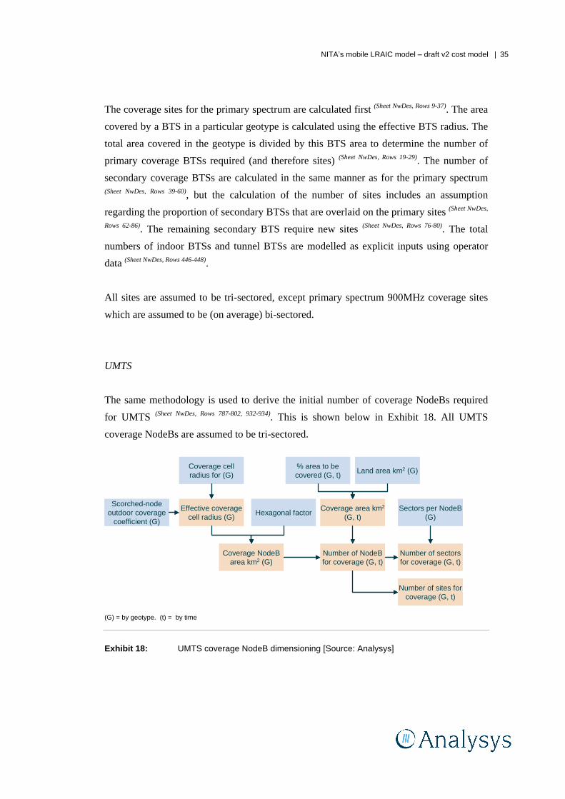
UMTS
The same methodology is used to derive the initial number of coverage NodeBs required
for UMTS (Sheet NwDes, Rows 787-802, 932-934). This is shown below in Exhibit 18. All UMTS
coverage NodeBs are assumed to be tri-sectored.
Land area km2 (G)% area to be covered (G, t)
Coverage area km2
(G, t)Effective coverage
cell radius (G)
Coverage NodeBarea km2 (G)
Hexagonal factor
Number of NodeBfor coverage (G, t)
Number of sites for coverage (G, t)
Sectors per NodeB(G)
Number of sectors for coverage (G, t)
Scorched-node outdoor coverage
coefficient (G)
Coverage cell radius for (G)
(G) = by geotype. (t) = by time
Exhibit 18: UMTS coverage NodeB dimensioning [Source: Analysys]

NITA s mobile LRAIC model
draft v2 cost model | 36
Within the UMTS network, however, the effect of cell breathing has been included. Cell
breathing takes places in a UMTS network in the situation where traffic loads increase and
the subsequent rise in the signal-to-noise ratio acts to curtail the range of the cell
usually
anticipated to be limited by the uplink communication. The coverage cell radii inputs to the
model are estimated (using operator data and a number of link-budget calculations) to be
applicable for up to a 50% load on the cells in the network. Beyond a 50% cell load, the
cell radius is estimated to decline using a polynomial approximation shown in Exhibit 19
below.
y = -2.3781x2 + 2.6013x + 0.2932
0.00
0.20
0.40
0.60
0.80
1.00
1.20
0% 20% 40% 60% 80% 100%
Cell load
Rel
ativ
e ce
ll ra
dius
Radius Max (100%) load Poly. (Radius)
Exhibit 19:
Estimated cell
breathing effect
[Source: Analysys]
The cell load is calculated (by geotype) in the model according to the average number of
utilised carriers per sector (Sheet NwDes, Rows 1000-1003), which is then applied to the polynomial
approximation to give the relative cell radius factor. Since the cells are shrinking at the
edges, and the uncovered area cannot be uniquely covered by single additional sites in each
locality, the relative cell radius factor is squared once, to reflect the area per site, and then
squared again to reflect the degree of infill coverage required to cover the hexagonal
mesh of uncovered areas (Sheet NwDes, Rows 1014-1017). In order to avoid a complicated circularity
in the model, the cell radius post-cell-breathing is applied to the following year s coverage
roll-out calculation (Sheet NwDes, Rows 790-794).

NITA s mobile LRAIC model
draft v2 cost model | 37
6.2 Radio network: site capacity requirement (GSM and UMTS)
The capacity requirements for each technology (primary GSM, secondary GSM and
UMTS) are calculated separately within the model. In all cases, two steps are required,
which involve calculating
The capacity provided by the coverage sites (Sheet NwDes, Rows 186-215, 853-864).
The number of additional sites (including secondary spectrum overlays, if available)
required to fulfil capacity requirements (Sheet NwDes, Rows 217-271, 866-888).
However, the differences between GSM and UMTS technologies means that the
methodologies require slightly different inputs, as explained below.
GSM capacity requirements
Step 1: Capacity provided by the sectorised coverage sites
Denmark has coverage requirements for both its GSM900 and GSM1800 licences. Section 6.1
explains how the number of coverage BTSs has been derived for the three 2G operators, by
geotype, technology and over time. The calculation of the busy-hour Erlang (BHE) capacity
provided by the sites deployed for coverage purposes is shown in Exhibit 20.

NITA s mobile LRAIC model
draft v2 cost model | 38
Spectrum channels(t, 900MHz, 1800MHz)
Spectrum MHz (t, 900MHz, 1800MHz)
MHz per channel (900MHz,1800MHz)
Radio blocking probability (t, 900MHz, 1800MHz)
Maximum sector re-use (900MHz,1800MHz)
Spectral sector capacity (TRX) (t, 900MHz, 1800MHz)
Physical capacity of BTS in TRX (G)
Actual sector capacity (TRX) (G, t, 900MHz, 1800MHz)
Erlangs required for a given number of channels (G)
Actual sector capacity (Erlang) (G, t, 900MHz,
1800MHz)
Sectors required for coverage (G, 900MHz, 1800MHz)
Peak TRX utilisation
Coverage sector capacity (BHE) (G, t, 900MHz,
1800MHz)
Total coverage capacity (BHE) (G, t)
Peak macro BTS utilisation (900MHz,1800MHz)
Inputs are broken down by geotype (G), by time (t), or by frequency band
Exhibit 20: Calculation of the BHE capacity provided by the coverage network [Source:
Analysys]
For each GSM operator, the coverage capacity for each technology is calculated separately. For
a given technology, before the capacity requirements of the network are calculated, the Erlang
capacity for the allocated spectrum is determined.
The inputs to this calculation are:
Availability of spectrum,
spectrum re-use factor,
blocking probability, and
BTS capacity, in terms of TRXs.

NITA s mobile LRAIC model
draft v2 cost model | 39
The spectral capacity per sector is the number of transceivers that can be deployed per
sector given a certain maximum spectrum re-use factor. The lesser of the physical capacity
and the spectral capacity of a sector is the applied capacity (Sheet NwDes, Rows 124-168).
The sector capacity in Erlangs is obtained using the Erlang B conversion table
channel
reservations for signalling and GPRS are made in the Erlang B table according to the
information provided by the operators. In calculating the effective capacity of each sector
in the coverage network, allowance is made for the fact that BTSs and TRXs will in fact be
underutilised:
Underutilisation of BTSs occurs because it is not possible to deploy the full physical
TRX complement in every BTS, since BHE demand does not occur uniformly at a
small number of sites. Alternatively, an operator may specifically choose to provide
capacity using additional sites rather than additional TRXs.
Underutilisation of TRXs occurs because the peak loading of each cell at its busy hour
is greater than the network average busy hour. To take this into account, an average-to-
peak BHE-loading factor of 150% is used in the calculation of TRX utilisation,
accounting for the fact that the cell busy hour is 50% greater than the network busy
hour. Also, BHE demand does not uniformly occur in a certain number of sectors.
This sector capacity (in Erlangs) is then multiplied by the total number of sectors in the
coverage network to arrive at the total capacity of the network.
Step 2: Calculation of the number of additional sites required to fulfil capacity
requirements
It is assumed that all the GSM operators only deploy capacity BTSs on new sites, rather
than overlaying existing sites. This is based on comparison of the versions of the mast
database for the period 2003 06, which indicate that almost all of the incremental GSM
BTSs deployed were on completely new sites, either as single-technology sites or dual
sites. The reason for this is likely to be that (respectively):
TDC and Sonofon will not overlay on existing coverage sites because their 1800MHz
coverage is inside their 900MHz coverage, so they will already have overlaid those

NITA s mobile LRAIC model
draft v2 cost model | 40
sites for 1800MHz coverage reasons in the high-population areas where the new traffic
loads will be located.
Telia accommodates increasing capacity with 1800MHz and uses 900MHz to extend
rural coverage. For this reason, increasing demand is occurring in places (i.e.
population centres) where the operator already has 1800MHz sites.
Therefore, the additional sites required are calculated to fulfil capacity requirements after
the calculation of the capacity of the coverage networks, as shown below in Exhibit 21.
Radio BHE (G,t)
BHE carried over coverage network (BHE)
(G, t)
BHE requiring additional radio site capacity (G, t)
Total coverage capacity (BHE) (G, t)
Peak macro BTS utilisation
TRX utilisation
Sectors per BTS (3 for full sectorisation)
Actual spectrum capacity (Erlang) (G, t)
Total effective capacity of fully overlaid site (G, t)
Proportion of additional sites (G)
Average capacity per additional site (G, t)
Additional sites required (G, t)
Total capacity BTS (G, t)
(G) = by geotype. (t) = by time
Exhibit 21: Calculation of the additional sites required to fulfil capacity requirements [Source:
Analysys]
Three types of GSM site are dimensioned according to the spectrum employed:
Primary-only sites.
Secondary-only sites.
Dual sites.
The total BHE demand is aggregated by element and then re-partitioned by geotype. GPRS
traffic is currently excluded, on the assumption that it is carried in a channel reservation.
Knowing the total capacity of the coverage network allows the determination of the BHE

NITA s mobile LRAIC model
draft v2 cost model | 41
demand that cannot be carried by the coverage network, broken down by geotype (Sheet NwDes,
Rows 219-222).
Assuming that all new sites are fully sectorised and that both BTSs and TRXs are not fully
utilised, the total effective capacity of a fully sectorised BTS for both primary and
secondary spectrum is calculated (Sheet NwDes, Rows 226-235). Then, for a selected operator, it is
assumed that new GSM sites will be deployed in specific proportions by site type (Sheet NwDes,
Rows 237-241). These parameters are used with the effective BTS capacities to calculate the
weighted average capacity per additional site by geotype. The total BHE demand not
accommodated by the coverage networks is then used, along with this weighted average
capacity and the split of new sites by site type, to calculate the number of additional sites
by site type and geotype required to accommodate this residual BHE (Sheet NwDes, Rows 250-271).
UMTS capacity requirements
Step 1: Capacity provided by the sectorised coverage sites
Exhibit 22 below demonstrates the methodology used to derive the capacity of the UMTS
network.

NITA s mobile LRAIC model
draft v2 cost model | 42
Available channel
elements per sector (t)
Percentage of channels reserved for
signalling/soft-handovers
16 channel elements per channel kit
5 channel kit per carrier per sector, 3 sectors per
NodeB
Channel elements required per sector (G)
Channels available per sector to carry voice/data
(G, t)
Erlang B Table
Erlang channels available per sector to carry voice/data (G, t)
Voice and guaranteed data (BHE)
Weighted average BHE channel load (t)
BHE traffic split (G)Voice BHE traffic (Erlangs) (G, t)
Capacity on coverage network (G, t)
UMTS coverage BTS (G, t)
BHE traffic supported by coverage network (G, t)
BHE traffic not supported by coverage network (G, t)
Radio network blocking probability (1%)
Channel kit utilisation
NodeB utilisation
Available channel elements per sector (t)
Percentage of channels reserved for
signalling/soft-handovers
16 channel elements per channel kit
5 channel kit per carrier per sector, 3 sectors per
NodeB
Channel elements required per sector (G)
Channels available per sector to carry voice/data
(G, t)
Erlang B Table
Erlang channels available per sector to carry voice/data (G, t)
Voice and guaranteed data (BHE)
Weighted average BHE channel load (t)
BHE traffic split (G)Voice BHE traffic (Erlangs) (G, t)
Capacity on coverage network (G, t)
UMTS coverage BTS (G, t)
BHE traffic supported by coverage network (G, t)
BHE traffic not supported by coverage network (G, t)
Radio network blocking probability (1%)
Channel kit utilisation
NodeB utilisation
(G) = by geotype. (t) = by time
Exhibit 22: Calculation of the BHE capacity provided by the UMTS coverage network
[Source: Analysys]
The following assumptions about specific 3G modelling inputs have been made:
3 sectors per NodeB.
5MHz per UMTS carrier.
A maximum physical capacity of 5 channel kit per carrier per sector, across all
geotypes-
Channel elements are pooled at the NodeB.
16 channel elements per channel kit.
1 channel element required to carry a voice call; 4 to carry a video call.
30% of channel elements are reserved for signalling/soft-handover purposes.

NITA s mobile LRAIC model
draft v2 cost model | 43
The model ensures that all offered traffic
voice, data and video
is carried with a
guarantee of available bandwidth. This represents the situation where delivery of best-
effort data traffic is undertaken without compromise to the user s experience of the service
during the busy hour. The degree to which operators may allow degradation in packet data
service during the busy hour is highly uncertain at the current time, and HSDPA services
may be available to more efficiently deliver down-link traffic. Therefore, the model
includes the option to exclude 3G packet data from the radio dimensioning part (Sheet
Control.Panel, Row 23), or to specify the directionality of the capacity-limited 3G bearer (i.e. an
uplink or downlink percentage in the 3G PS data Erlang calculation) (Sheet Control.Panel, Row 24).
The sector capacity (in Erlangs) is then obtained using the Erlang B conversion table and,
using the 3G demand data in BHE calculated by the model, the average BHE channel load
is obtained. Operator data has also allowed the model to estimate 3G BHE split by geotype
(with indoor traffic calculated separately).
The number of UMTS coverage sites calculated earlier in the model is multiplied by the
average BHE channel load to derive the capacity in the coverage network by geotype (Sheet
NwDes, Rows 866-870). However, as when modelling GSM capacity requirements, allowance is
made for the fact that NodeB and channel kit capacity is less than 100% utilised:
Underutilisation of NodeBs occurs because it is not possible to deploy the full physical
complement of channel kit in every NodeB, since BHE demand does not uniformly
exist at a small number of sites. Alternatively, an operator may choose to satisfy
capacity load with additional NodeBs rather than additional channel kit for each
existing carrier.
Underutilisation of channel kit occurs because the peak loading of each cell in its busy
hour is greater than the network average busy hour. To take this into account, the same
average-to-peak BHE-loading factor of 150% is used in the calculation of the channel
kit utilisation, i.e. the cell busy hour is assumed to be 50% greater than the network
busy hour. Also, BHE demand does not uniformly occur in a certain number of NodeB
sectors.

NITA s mobile LRAIC model
draft v2 cost model | 44
Step 2: Calculation of the number of additional sites required to fulfil capacity
requirements
Having calculated both the 3G BHE and the capacity of the coverage network by geotype,
the BHE that cannot be accommodated by the coverage network by geotype is derived (Sheet
NwDes, Rows 872-876), and the number of additional sites calculated, as shown below in Exhibit 23.
Capacity on coverage network (G, t)
BHE traffic supported by coverage network (G, t)
BHE traffic not supported by coverage network (G, t)
BHE traffic that can be supported by additional carrier
on coverage sites (G, t)
Capacity on single-carrier coverage network (G, t)
Weighted average BHE channel load (t)
Effective capacity of a site with a full overlay (t)
BHE traffic that cannot be supported by an additional
carrier on coverage sites (G, t)
Coverage sites which are overlaid (G, t)
Number of additional sites required (G, t)
Channel kit utilisation
NodeB utilisation
(G) = by geotype. (t) = by time
Exhibit 23: Calculation of the additional sites required to fulfil capacity requirements [Source:
Analysys]
This calculation essentially uses a three-stage algorithm:
Stage 1: If the 3G BHE in a geotype can be accommodated by the coverage network
for that geotype, then no further carriers or sites are added to the network.

NITA s mobile LRAIC model
draft v2 cost model | 45
Stage 2: If the 3G BHE in a geotype cannot be accommodated by the coverage
network for that geotype, then another carrier is added to the BTS in that geotype so
that the residual 3G BHE can be accommodated.
Stage 3: If the proportion in Stage 2 reaches 100% (so every 3G coverage BTS in that
geotype has been overlaid with additional carriers) and there is still more 3G BHE in
that geotype, then the number of additional sites required in that geotype to
accommodate the residual BHE from Stage 1 and Stage 2 is calculated. These
additional sites are assumed to be deployed fully overlaid (with 2 carriers used) (Sheet
NwDes, Rows 878-894).
6.3 Radio network: TRX requirements
To calculate the total number of transceivers required, the inputs required are:
BHE traffic.
Number of GSM sectors, split between 900MHz and 1800MHz.
Transceiver utilisation.
Minimum number of TRXs per sector, which is assumed to be
2 in the urban geotypes
1 in the rural geotype
1 or 2 for special sites (indoor and tunnel sites) depending on operator-stated data
Blocking probability for the radio network.
Exhibit 24 below gives a flow diagram describing the calculation of transceivers required.

NITA s mobile LRAIC model
draft v2 cost model | 46
Total sectors (G, t,
1800MHz, 900MHz)BHE traffic (G, t, 1800MHz,
900MHz)
Average BHE traffic per sector (G, t, 1800MHz, 900MHz)
Radio network blocking probability
Minimum TRX per sector (G, 1800MHz, 900MHz)
Maximum utilisation of TRX erlang capacity
TRX per sector to meet traffic requirements (G, t, 1800MHz,
900MHz)
Total number of TRXs required (G, t, 1800MHz, 900MHz)
Total sectors (G, t, 1800MHz, 900MHz)
BHE traffic (G, t, 1800MHz, 900MHz)
Average BHE traffic per sector (G, t, 1800MHz, 900MHz)
Radio network blocking probability
Minimum TRX per sector (G, 1800MHz, 900MHz)
Maximum utilisation of TRX erlang capacity
TRX per sector to meet traffic requirements (G, t, 1800MHz,
900MHz)
Total number of TRXs required (G, t, 1800MHz, 900MHz)
(G) = by geotype. (t) = by time
Exhibit 24: Transceiver deployment [Source: Analysys]
The number of TRXs required in each sector to meet the demand is calculated taking into
consideration the TRX utilisation, and converting the Erlang demand per sector into a
channel requirement using the Erlang B table and the assumed blocking probability. The
TRXs for each sector are then calculated (being at least the minimum amount specified
above), and then the total number of TRXs required is obtained by multiplying the number
of sectors and the number of TRXs per sector (Sheet NwDes, Rows 512-631).
6.4 Backhaul transmission
The calculation of the number of backhaul links and the corresponding number of E1 ports
required is set out in Exhibit 25 below.

NITA s mobile LRAIC model
draft v2 cost model | 47
Circuits (G,t)
Total number of macro sites (G, t)
Special sites (t)
1 leased E1 per Special site
Proportion of sites using microwave (G)
Proportion of sites using leased lines (G)
E1 utilisation
E1s per site (G, t)
Number of sites using E1 links (G, t)
Number of microwave links (2Mbit/s) (G, t)
Total number of E1links (G, t)
Number of E1s occupied (G, t)
Proportion of sites directly linked to the fibre
ring (G) Number of E1 links connected into Fibre to
BSC links
E1s per site (G, t)
Total number of E1 links required for special sites
(t)
(G) = by geotype. (t) = by time
Exhibit 25: Backhaul calculation [Source: Analysys]
Step 1: Capacity requirements
The number of E1s required per macro site is calculated to fulfil the capacity requirements
for a backhaul link. There are eight channels per transceiver, which translates into eight
circuits in the backhaul since the backhaul is dimensioned to support all the TRX channels.
If an operator has deployed EDGE in its radio network, the relevant number of reserved
TRX channels are multiplied by a factor of four (representing the 4x coding gain achieved
with EDGE). Taking into consideration the co-location of primary and secondary BTSs on
the same site, the number of channels per site is calculated on the basis of the number of

NITA s mobile LRAIC model
draft v2 cost model | 48
channels per TRX multiplied by the number of 900MHz and 1800MHz TRXs. Given the
maximum capacity of an E1 link and considering the link utilisation, the effective capacity
per E1 link is calculated. The number of E1 links required per site is then obtained by
simply dividing the circuits per site by the actual capacity per E1 link (Sheet NwDes, Rows 653-668).
Step 2: Backhaul network design algorithms
There are two types of backhaul to be considered in the network: microwave (2Mbit/s
links) and leased line backhaul. The percentage of sites which have microwave backhaul is
an input into the model.
The number of microwave backhaul links (capacity of 8Mbit/s or four E1 equivalents) is
set to be a minimum of one per site. The model allows for more than one 2Mbit/s link to be
deployed in the microwave link (Sheet NwDes, Rows 670-682).
The number of sites using leased lines is calculated as the difference between the total sites
and the number of sites using microwaves. The number of E1 leased lines required is
obtained by multiplying the total number of macro sites using leased lines by the average
number of E1s required per site (from Step 1) (Sheet NwDes, Rows 684-696).
A defined proportion of sites are linked to the BSC via the fibre ring network. The capacity
of these links is dimensioned according to the average number of E1s per site (by geotype) (Sheet NwDes, Rows 701-709).
Special sites (indoor and tunnel sites) are assumed to use only E1 leased-line backhaul and
hence are added to the leased-line requirement of the macro layer (Sheet NwDes, Rows 698-699).
6.5 BSC deployment
The structure of the BSC deployment algorithm is set out below in Exhibit 26.

NITA s mobile LRAIC model
draft v2 cost model | 49
BSC capacity in TRX
Maximum utilisationTRX (G,t)
Number of BSC required (G,t)
Total number of BSC (G,t)
MSC-facing E1 ports per BSC (G,t)
BSC-MSC BHE (G,t)Total number of MSC-facing BSC E1 ports (t)
BSC capacity in TRX
Maximum utilisationTRX (G,t)
Number of BSC required (G,t)
Total number of BSC (G,t)
MSC-facing E1 ports per BSC (G,t)
BSC-MSC BHE (G,t)Total number of MSC-facing BSC E1 ports (t)
Exhibit 26:
BSC
deployment
[Source:
Analysys]
(G) = by geotype. (t) = by time
Calculation of BSC units
The number of BSC units deployed is dependent on the capacity of a BSC, its utilisation
and the total number of TRXs required. The number of BSC units deployed must be able to
accommodate the number of TRXs deployed (see Section 6.3). Given a maximum capacity
of the BSC in terms of TRXs, adjusted for maximum utilisation, the number of BSCs
required is calculated (Sheet NwDes, Rows 716-731).

NITA s mobile LRAIC model
draft v2 cost model | 50
Calculation of BSC MSC links
Remote BSCs (G,t)
BSC-MSC BHE (G,t)BSC-MSC BHE per remote BSC (G,t)
E1 capacity and utilisation
Number of E1 links (G,t)
Exhibit 27:
BSC MSC remote
transmission
[Source: Analysys]
(G) = by geotype. (t) = by time
A proportion of BSCs are designated remote (i.e. not co-located with an MSC), and
therefore require physical links to the MSC. The traffic transiting through these BSCs is
backhauled to the MSC using E1 leased lines (on the fibre ring network).
The total traffic handled by each remote BSC can be calculated using the total BHE
transceiver traffic. The average BHE traffic handled by each remote BSC is converted into
a channel requirement using the Erlang table. The number of E1 links is then calculated by
dividing this channel requirement by the capacity of an E1 link, adjusted for maximum
utilisation. It should be noted that the capacity of the BSC MSC transmission depends on
where the transcoder equipment is located. For remote BSCs, the transcoder is assumed to
be located in the MSC, and so, according to the GSM standard, has a capacity of 120
circuits. (Sheet NwDes, Rows 733-739, 751-761)
The number of E1 BSC MSC ports is determined on the basis of the number of BSC MSC
E1 links (Sheet NwDes, Row 765).

NITA s mobile LRAIC model
draft v2 cost model | 51
Total outgoing ports for co-located BSCs
Given the total number of co-located BSCs and BHE transceiver traffic, the total number of
outgoing ports for co-located BSCs is calculated (Sheet NwDes, Rows 767-779). The flow of
calculation for co-located BSC ports is similar to that shown in Exhibit 27, except that the
transcoder is assumed to be in the BSC (and therefore the E1 capacity is 30 channels) and
the co-located links are not modelled (because this is part of the in-building cat-5 or similar
wiring).
Incoming and outgoing ports
The incoming ports to the BSC are ports facing the BTS while the outgoing ports are ports
facing the MSC. The diagram below shows the constituents of the incoming and outgoing
ports.
Total E1 incoming ports
Number of E1 for remote BSC-MSC links
Incoming ports Outgoing ports
Number of occupied E1 units of 8Mbit/s backhaul
Number of leased line E1 links
Number of E1 for co-located BSC-MSC links
Total E1 outgoing portsTotal E1 incoming ports
Number of E1 for remote BSC-MSC links
Incoming ports Outgoing ports
Number of occupied E1 units of 8Mbit/s backhaul
Number of leased line E1 links
Number of E1 for co-located BSC-MSC links
Total E1 outgoing ports
Exhibit 28: Total incoming and outgoing ports for BSC [Source: Analysys]
The total number of E1 incoming ports into a BSC is the sum of the microwave and leased
line backhaul links, while the total outgoing ports is the sum of the total number of E1s for
both remote and co-located BSCs (Sheet NwDes, Rows 742-749).

NITA s mobile LRAIC model
draft v2 cost model | 52
6.6 3G NodeB deployment
The 3G NodeB deployment algorithm is outlined in Section 6.2.
6.7 3G channel kit and carriers deployment
The dimensioning of 3G channel kit is done in a similar manner to the calculation of 2G
TRXs (Sheet NwDes, Rows 941-1000), with the exception that an allowance is made for soft handover:
Total number of UMTS sites (G, t)
UMTS BHE traffic per geotype (G, t)
Average BHE traffic per site (G, t)
Radio network blocking probability (1%)
Minimum CK per site (G)
Maximum utilisation of CE erlang capacity
CK per site to meet traffic requirements including a soft-
handover allowance (G, t)
Total number of CK required (G, t)
Channel Elements per Channel Kit
Soft-handover allowance
Total number of UMTS sites (G, t)
CK per site to meet traffic requirements including a soft-
handover allowance (G, t)
CK per carrier per Node B
Minimum number of carriers per Node B
Number of carriers required per Node B
Total number of UMTS sites (G, t)
UMTS BHE traffic per geotype (G, t)
Average BHE traffic per site (G, t)
Radio network blocking probability (1%)
Minimum CK per site (G)
Maximum utilisation of CE erlang capacity
CK per site to meet traffic requirements including a soft-
handover allowance (G, t)
Total number of CK required (G, t)
Channel Elements per Channel Kit
Soft-handover allowance
Total number of UMTS sites (G, t)
CK per site to meet traffic requirements including a soft-
handover allowance (G, t)
CK per carrier per Node B
Minimum number of carriers per Node B
Number of carriers required per Node B
(G) = by geotype. (t) = by time
Exhibit 29: 3G channel kit and carrier dimensioning [Source: Analysys]

NITA s mobile LRAIC model
draft v2 cost model | 53
6.8 3G backhaul deployment
3G backhaul is dimensioned in the same way as 2G backhaul (Sheet NwDes, Rows 1020-1103). 3G
backhaul is assumed to be logically and physically separate from 2G backhaul from the site
to the switch.
6.9 3G RNC deployment
RNCs are dimensioned on the basis of the number of NodeBs per RNC, and the total traffic
in the radio network.
RNC capacity in NodeBs
Maximum utilisation
NodeBs (G,t)
Number of RNC required to support NodeBs (G,t)
Total number of RNC (G,t)
Minimum number of RNC
RNC traffic capacity
Traffic BHE
Utilisation factor
RNCs required for CS traffic
(G) = by geotype. (t) = by time
Exhibit 30: RNC dimensioning [Source: Analysys]
A minimum number of RNC units are modelled
this minimum deployment of 1 or 2
RNCs is based on operator data (Sheet NwDes, Rows 1105-1103).
The number of E1 ports into and out of RNCs is modelled in the same way as for BSC
switches (Sheet NwDes, Rows 1123-1145).

NITA s mobile LRAIC model
draft v2 cost model | 54
6.10 2G MSC deployment
Calculation of number of MSC units to support processing demand
To support processing demand, the number of MSC units required is calculated from the
CPU capacity, processor utilisation and the demand for MSC processor time. The flow
diagram below shows the sequence of the calculation.
MSC CPU CapacityMSC Processor
UtilisationTotal BHms Demand for
MSC (t)
Required number of processors for BHms
demand (t)
MSC Processor Capacity
MSC Units required to support processor BHms
demand (t)
(t) = by time
Exhibit 31: Calculation of MSC units to support processing demand [Source: Analysys]
Taking into account the MSC processor utilisation, the total number of processors required
to meet the demand can be calculated as the total number of busy-hour milliseconds
(BHms) divided by the effective MSC capacity (Sheet NwDes, Rows 1154-1163).
Calculation of TSCs, MSC locations, logical links and physical links
TSCs, MSC locations, logical links and physical links are all calculated by means of a
reference table based on the number of MSCs deployed in an operator s network. This
reference table
shown in Exhibit 32 below
is based directly on operator s submitted
data, and is specific to the Danish network topology (Sheet NwDes, Rows 1166-1181).
The number of MSC locations is obtained by averaging the deployment for all operators. A
transit layer of 2 TSC switches is assumed to be required when the number of MSCs
reaches 10 in order to reduce the complexity of the logical transmission layout.

NITA s mobile LRAIC model
draft v2 cost model | 55
# MSC 0 1 2 3 4 5 6 7 8 9 10 11 12 13 14 15 16
# MSC locations 0 1 2 3 3 4 5 6 6 6 6 6 6 7 8 9 10# TSC 0 0 0 0 0 0 0 0 0 0 2 2 2 2 2 2 2# Logical E1 routes 0 0 2 3 3 6 10 15 15 15 12 12 12 16 20 25 30# Physical routes 0 6 6 6 6 6 7 8 8 8 8 8 8 9 10 11 12# Rings 0 3 3 3 3 3 3 3 3 3 3 3 3 3 3 3 3Physical routes by ring Sjealland 0 2 2 2 2 2 3 3 3 3 3 3 3 4 4 5 5
Fyn 0 2 2 2 2 2 2 2 2 2 2 2 2 2 3 3 3Jutland 0 2 2 2 2 2 2 3 3 3 3 3 3 3 3 3 4
Distribution of E1 per ring Sjealland 0% 0% 0% 0% 50% 50% 50% 50% 50% 50% 50% 50% 50% 50% 50% 50% 50%Fyn 0% 0% 100% 50% 25% 25% 25% 25% 25% 25% 25% 25% 25% 25% 25% 25% 25%Jutland 0% 0% 0% 50% 25% 25% 25% 25% 25% 25% 25% 25% 25% 25% 25% 25% 25%
Ring length (km) Sjealland 50Fyn 600Jutland 400
Exhibit 32: Core network reference table [Source: Analysys]

NITA s mobile LRAIC model
draft v2 cost model | 56
The calculation of the number of logical links that are required is based on the fully-meshed
formula n(n-1)/2 where n is the number of MSC locations. This is shown in Exhibit 33.
1
2
1
2
3
1
2
3
45
6
0 logical routes
2 logical routes
3 logical routes
6 logical routes
10 logical routes
15 logical routes
1
2
1
2
1
2
3
1
2
3
1
2
3
45
6
1
2
3
45
6
0 logical routes
2 logical routes
3 logical routes
6 logical routes
10 logical routes
15 logical routes
Exhibit 33:
Logical route
dimensioning of the
backbone [Source:
Analysys]
When dimensioning physical routes, a topology of three linking fibre rings is used, with
rings deployed on each of the three main parts of Denmark (see Exhibit 16 on page 29
above). The topology modelled is based on information sourced from each operator. The
model always deploys the three fibre rings, although there may be zero or one MSC MSC
route
in which case the fibre rings serve the sole purpose of backhauling site and
BSC/RNC traffic back to the main switching centre(s). Based on this three-ring
architecture, the number of physical links can be determined, as shown in Exhibit 34
below.

NITA s mobile LRAIC model
draft v2 cost model | 57
1
2
3
0 physical routes
2 physical routes
4 physical routes
6 physical routes
7 physical routes
8 physical routes
1
2
4
3
1
2
4
56
3
1
2
4
56
7
3
1
2
4
5
6
7
8
1
2
3
0 physical routes
2 physical routes
4 physical routes
6 physical routes
7 physical routes
8 physical routes
1
2
4
3
1
2
4
56
3
1
2
4
56
7
3
1
2
4
5
6
7
8
Exhibit 34
Physical route
dimensioning of the
backbone [Source:
Analysys]
Given that Copenhagen is on Zealand, the model assumes that a higher proportion of the
E1 inter-switch links are located on the Zealand fibre ring. The remaining E1 links are
divided equally between the Funen and Jutland fibre rings. This is shown in Exhibit 32
above.
Calculation of BSC-facing, interconnect-facing, VMS-facing and core-facing ports
Exhibit 35 below shows how the number of incoming and outgoing ports is obtained.

NITA s mobile LRAIC model
draft v2 cost model | 58
MSC locations (t)
Interconnection BHE traffic (t)
Interconnection traffic per MSC location
Erlang table channel calculation
Interconnection traffic per MSC location
(channels) (t)
Interconnection port utilisation
E1 capacity (circuits)
Interconnection ports per location (E1s) (t)
MSC locations (t)Number of
interconnection- facing E1 ports required (t)
Interconnect infrastructure VMS ports
Voicemail BHE traffic (t)
Erlang table channel calculation
Voicemail traffic (channels) (t)
Port utilisation
E1 capacity (circuits)
VMS ports (E1s) (t)
Incoming ports
Total number of outgoing E1 ports from BSCs (t)
Total number of incoming E1 ports from
BSCs (t)
(t) = by time
Exhibit 35: Calculation of BSC-facing, interconnect-facing and VMS-facing ports [Source:
Analysys]
The total number of incoming ports in the MSC is simply taken as the total number of E1
outgoing ports from the BSC (Sheet NwDes, Rows 1150-1152).
The total number of outgoing ports comprises the number of interconnect-facing ports
required, the number of VMS-facing ports required (both shown conceptually in Exhibit 35
above), plus the number of inter-switch ports required.
For the interconnection infrastructure, the total number of interconnect-facing ports
required to meet demand is obtained by dividing the interconnection BHE traffic at each
MSC location (as a channel requirement) by the actual E1 capacity of the port (Sheet NwDes,
Rows 1194-1202).
Inter-switch links are dimensioned on the basis of the BHE inter-switch traffic per logical
route (the number of which is determined according to the MSC reference table) (Sheet NwDes,
Rows 1212-1219).

NITA s mobile LRAIC model
draft v2 cost model | 59
6.11 Calculation of length of backbone links
The length of the backbone ring network is determined on the basis of the inter-switch
physical routes
refer to Exhibit 34 for the dimensioning of these routes on the basis of
MSC locations. As discussed previously, the model assumes that a higher proportion of the
E1 inter-switch links are on the Zealand fibre ring, with the remainder divided between the
Funen and Jutland fibre rings on the basis of the number of physical links dimensioned.
The backbone is dimensioned in terms of STM-1 links, where one STM-1 link contains 63 E1
links, subject to a maximum utilisation factor. An average route length per physical route is
calculated in order to determine the backbone link length required and the number of links (Sheet
NwDes, Rows 1221-1252).
6.12 Transit layer deployment
The deployment of a transit layer is determined according to the MSC reference table
outlined in Exhibit 32. Two TSC units are deployed when at least 10 MSCs (deployed in 6
MSC locations) are deployed in the network. By deploying a transit layer, the number of
logical links that are required is reduced compared to a fully-meshed network, e.g. the
network is split into two sets of fully-meshed linkages (linked through the TSCs). This is
shown in Exhibit 36 for the case of MSCs in seven locations with two TSCs.
MSC location
TSC
6 logical routes 10 logical routes
7 locations
mesh 1
mesh 2
Exhibit 36:
Two-mesh linking
for transit layer
[Source: Analysys]
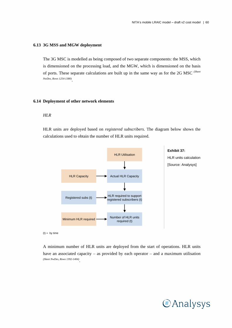
NITA s mobile LRAIC model
draft v2 cost model | 60
6.13 3G MSS and MGW deployment
The 3G MSC is modelled as being composed of two separate components: the MSS, which
is dimensioned on the processing load, and the MGW, which is dimensioned on the basis
of ports. These separate calculations are built up in the same way as for the 2G MSC (Sheet
NwDes, Rows 1254-1380).
6.14 Deployment of other network elements
HLR
HLR units are deployed based on registered subscribers. The diagram below shows the
calculations used to obtain the number of HLR units required.
HLR Capacity
HLR Utilisation
Actual HLR Capacity
Registered subs (t)HLR required to support registered subscribers (t)
Minimum HLR requiredNumber of HLR units
required (t)
Exhibit 37:
HLR units calculation
[Source: Analysys]
(t) = by time
A minimum number of HLR units are deployed from the start of operations. HLR units
have an associated capacity
as provided by each operator
and a maximum utilisation (Sheet NwDes, Rows 1392-1404).

NITA s mobile LRAIC model
draft v2 cost model | 61
SMSC
The SMSC deployment is driven by SMS throughput demand. The diagram below shows
the calculation flow.
SMSC Throughput Capacity
SMSC Utilisation
Actual SMSC Capacity
SMS Throughput Demand (t)
SMSCs required to support thoughput
demand (t)
Minimum SMSC unitsNumber of SMSC units
required (t)
Exhibit 38:
Calculation of SMSC
units [Source:
Analysys]
(t) = by time
Dividing the SMS throughput demand by the actual SMSC capacity gives the number of
SMSCs required to support this throughput demand. The number of SMSC units deployed
is the higher of either the SMSCs required to support demand or the minimum SMSC units (Sheet NwDes, Rows 1407-1419).
GPRS/EDGE/UMTS packet data infrastructure
There are three packet data infrastructures deployed, namely PCU, SGSN and GGSN.
PCU units are added to the GSM BSCs to groom packet data to/from the radio
transmission. A certain number of PCUs are deployed per BSC. It is assumed that the
UMTS RNC intrinsically contains PCU functionality (Sheet NwDes, Rows 1424+).
The exhibit below shows the calculations for SGSN and GGSN deployment, supporting
connective and active packet data subscribers of both 2G and 3G networks.

NITA s mobile LRAIC model
draft v2 cost model | 62
SGSN/GGSN Capacity
SGSN/GGSN Utilisation
Actual SGSN/GGSN Capacity
Connected subscribers/active PDP
contexts in the busy hour (t)
SGSNs/GGSNs required to support BH connected
subs/PDP contexts (t)
Minimum SGSN/GGSN units
Number of SGSN/GGSN units required (t)
Exhibit 39:
SGSN and GGSN
units calculation
[Source: Analysys]
(t) = by time
The calculations for both SGSN and GGSN deployment are similar. SGSN deployment is
driven by the number of simultaneously connected subscribers in the busy hour (Sheet NwDes,
Rows 1431+), while GGSN deployment is driven by active PDP contexts made in the busy hour (Sheet NwDes, Rows 1442+). A minimum number of SGSNs and GGSNs must be deployed (one or
two, depending on operator data).
Network management centre
The network management centre is deployed at the start of operations (Sheet NwDes, Rows 1457).
Voicemail system, IN and billing system
These network elements are modelled as a single functional unit deployed at the
commencement of operations (Sheet NwDes, Rows 1460+).
Non-network elements
Major categories of non-network activities are also modelled:

NITA s mobile LRAIC model
draft v2 cost model | 63
Wholesale
overheads
The costs relating to the support of wholesale services is modelled
on the basis of the number of wholesale events carried by the
network. Wholesale events are considered to be the sum of:
incoming minutes from other networks
outgoing minutes from other networks
incoming SMS messages from other networks
outgoing SMS messages from other networks
national roaming minutes carried by own, or other networks.
Wholesale overheads are assumed to be operating expenditures
only.
Business overhead
activities
Business overhead activities include the head office, IT, personnel,
administrative support and executive management functions of the
business.
These activities may incur both capital and operating expenditures,
though the approach of each operator in capitalising or expensing its
business overhead expenditures varies according to how the
operator has chosen to deploy its mobile function in Denmark. As
such, the model allows for the following business overhead
expenditures:
one-off capital expenditure required to establish the head
office buildings and basic facilities
ongoing capital expenditure required to maintain and expand
the head office facilities, fixtures and fittings; modelled
approximately according to the number of subscribers supported
by the business
fixed annual operating expenditure of the fixed business
overhead functions of building rental and running costs,
business overhead staff salaries and executive management
costs
increasing annual operating expenditure of the expanding

NITA s mobile LRAIC model
draft v2 cost model | 64
business overhead support functions (facilities and salary
related costs); modelled approximately according to the number
of subscribers supported by the business.
2G licence fees Some operators specify 2G licence fees (annual operating
expenditures), which are modelled as a fixed annual expenditure.
3G licence fees The model includes the capital asset of the 3G licence fee; however,
its value is currently input as a notional DKK100. The expenditure
profile of this notional DKK100 is modelled as follows:
25% in year of purchase
7.5% per year for the following 10 years.

NITA s mobile LRAIC model
draft v2 cost model | 65
7 Expenditure calculations
Once the requirement for network assets over time has been calculated over time (Sheet
NwDeploy, Rows 9+), the model must compute the purchasing, replacement, retirement and
expenditures associated with these network elements.
7.1 Purchasing, replacement, and capex planning periods
The network design algorithms compute the network elements that are required to support
a given demand in each year (assessed at the year-average point). The network deployment
scheduled is smoothed with respect to demand up to the peak asset deployment number, to
remove any transient dips in the profile of assets needed over time (Sheet NwDeploy, Rows 315+).
In order for network elements to be operational when needed, they need to be purchased in
advance (Sheet NwDeploy, Rows 785+), in order to allow provisioning, installation, configuration and
testing before they are activated. This is modelled for each asset by inputting a planning
period of between zero (no planning required) and 24 months. This concept of a look-ahead
period is illustrated in Exhibit 40.
Time
Demand requirement (t)subject to max utilisation
Look-aheadperiod
Ord
erin
gP
urch
asin
gD
eplo
ymen
tT
estin
gA
ctiv
atio
n
Dep
loym
ent Purchase requirement
subject to look-ahead
Exhibit 40:
Look-ahead period
for asset purchase
[Source: Analysys]

NITA s mobile LRAIC model
draft v2 cost model | 66
In order to calculate the number of assets to be purchased in each year, the model computes
the number of additional assets that need to be installed to provide incremental capacity,
and also includes the amount of equipment that has reached the end of its lifetime and
needs to be replaced (Sheet NwDeploy, Rows 630+).
The average accounting lifetime of network elements has been calculated by taking into
consideration the information submitted by the mobile operators on the depreciation
periods applied to their network elements. In addition, an economic asset lifetime has been
estimated by Analysys and NITA, taking into account the expectations of asset replacement
under economic rather than accounting circumstances.
7.2 Retirement algorithm
When the demand for an asset is reduced, it can either be removed from the network, or
retained. An algorithm is used to model how particular assets are to be retired (Sheet NwDeploy,
Rows 469+). There will be a period of delay between the point at which the demand reduction
occurs, and the point at which the asset is decommissioned. This delay can vary from zero
(the asset is retired in the same year that the demand reduction occurs) up to 100 years (the
asset remains in the network until the end of the network s lifetime), as shown in the
following exhibits.
Retirement
delay period (yr)
Explanation
0 Asset numbers reduce directly in the year that demand reduction occurs
1 Asset reduction lags demand reduction by 1 year
2 Asset reduction lags demand reduction by 2 year
100 Assets are maintained in the network until the end of the network
Exhibit 41: Values
used for the
retirement delay
period [Source:
Analysys]

NITA s mobile LRAIC model
draft v2 cost model | 67
Time
Dep
loym
ent
Actual requirement according to
demand
t=1 t=2 t=100
Exhibit 42:
Retirement
algorithm options
[Source: Analysys]
The retirement algorithm is built into the model because there are various reasons why
assets may not be removed perfectly from the network with reducing demand
such as
uncertainty over migrating volumes, or requirements to maintain network quality for
remaining subscribers.
7.3 Equipment unit prices
The model includes a schedule of capital and operating expenditures for each network
element (Sheet CostScenario.Basecase), along with a price trend which reflects the price of modern
equivalent assets over time (Sheet CostTrends). This price evolution also provides an important
input into the economic depreciation calculation, as explained in Section 8.
Capital and operating expenditures relevant to each network element in the model are
derived from the input of unit price (in real 2006 DKK) and the price trend applying from
1992 onwards.
The input of unit price consists of a number of components, which can generally be
considered to be broadly similar (though not identical) for each network operator. Some
distinct inputs exist, for example, where detailed operator data is unavailable or there are
specific differences in the operators network architecture:
Direct capital
expenditure
The direct capital expenditure for a network element reflects the list
price to purchase and install one unit of equipment.

NITA s mobile LRAIC model
draft v2 cost model | 68
These inputs have been estimated from two main sources:
bottom-up price lists provided by a number of the mobile
operators (e.g. from internal budget planning, vendor estimates
or other internal bottom-up operator data)
Analysys estimates.
In addition, a small number of bottom-up equipment prices have
been estimated by direct comparisons with top-down data.
Indirect capital
expenditure
The indirect capital expenditure for each network element
represents the share of other capitalised costs associated with
network deployment: installation capital, tools, testing, vehicles,
network facilities, etc. The additional indirect capital expenditure
associated with each network element category is identified by
observing the discrepancies (if any) between actual top-down
expenditures and the sum of bottom-up direct capital
expenditures.
The indirect capital expenditure allowance is added as a percentage
to the direct expenditure.
Operating
expenditures for
certain (direct)
network elements
The operating expenditures associated with the direct costs of
certain network facilities are modelled as an input in DKK terms.
The specific network facilities considered in this manner are:
radio site rental
backhaul leased E1 transmission links
backbone leased/self-managed STM1 transmission kilometres
wholesale overhead cost per wholesale event
annual and per-subscriber business overhead expenditure
2G licence fees.
However, the majority of these direct cost inputs are derived from
the actual top-down operating expenditures of each network

NITA s mobile LRAIC model
draft v2 cost model | 69
operator.
Operating
expenditures as a
percentage of
capital
expenditure for
various (indirect)
assets
The remainder of the network element operating expenditures are
estimated from top-down data on the basis of a percentage of capital
expenditure per unit. This opex input is specified according to the
1992 capex values, although in subsequent years operating
expenditure per unit is calculated according to the opex price trend.

NITA s mobile LRAIC model
draft v2 cost model | 70
8 Annualisation of expenditure
This section describes the implementation of the economical depreciation algorithm used in
NITA s mobile cost model. It details both the economic rationale for using this algorithm
and the calculation steps. Further discussion of the appropriate mark-up mechanism can be
found in the model principles document.
8.1 The rationale for using economic depreciation
Economic depreciation is a method for determining a cost recovery that is economically
rational , in that it:
Reflects the underlying costs of production, and
reflects the output of network elements over their lifetime.
The first factor relates the cost recovery to that of a new entrant to the market, which would
be able to offer the services based on the current costs of production. The second factor
relates the cost recovery to the lifetime of a mobile business
in that investments and
other expenditures are in reality made throughout the life of the business (especially large,
up-front investments) on the basis of being able to recover them from all demand occurring
in the lifetime of the business. New entrants to the market would also be required to make
these large upfront investments, and recover costs over the lifetime in a similar fashion to
the existing operators. (This is based on the realistic assumption that new entrants to the
market face the same systemic barriers to entry as were faced by the existing operators, and
would not be able to instantaneously capture the entire market of an operator, i.e. the
market is less than fully contestable).
These two factors are not reflected in accounting-based depreciation, which simply
considers when an asset was bought, and over what period the investment costs of the asset
should be depreciated.
Fundamentally, the implementation of economic depreciation utilised in the model is based
on the principle that all (efficiently) incurred costs should be fully recovered, in an
economically rational way. An allowance for capital return earned over the lifetime of the

NITA s mobile LRAIC model
draft v2 cost model | 71
business, specified by the weighted average cost of capital (WACC), is also included in the
resulting costs.
8.2 Implementation of economic depreciation principles
The economic depreciation algorithm recovers all efficiently incurred costs in an
economically rational way by ensuring that the total of the revenues generated across the
lifetime of the business are equal to the efficiently incurred costs, including cost of capital,
in PV terms. More specifically, for every asset class, in every year, the algorithm recovers
the proportion of total cost (incurred across the lifetime of the business) that is equal to the
revenue generated in that year as a proportion of the total revenue generated (across the
lifetime of the business) in PV terms.
PV calculation
The calculation of the cost recovered through revenues generated needs to reflect the value
associated with the opportunity cost of deferring expenditure or revenue to a later period.
This is accounted for by the application of a discount factor on future cash flow, which is
equal to the WACC of the modelled operator.
The business is assumed to be operating in perpetuity, and investment decisions are made
on this basis. This means that it is not necessary to recover investments within a particular
time horizon, for example the lifetime of a particular asset, but rather throughout the
lifetime of the business. In the model, this situation is approximated by explicitly
modelling a period of 50 years. At the discount rate applied, the PV of one DKK in the last
year of the model is fractional and thus any perpetuity value beyond 50 years is regarded as
immaterial to the final result.

NITA s mobile LRAIC model
draft v2 cost model | 72
Cost recovery profile
The costs incurred over the lifetime of the network are recovered in line with the revenues
generated by the business. The revenues generated by an asset class are the product of the
demand (or output) supported by that asset class, and the price per unit demand.
In the modelled environment of a competitive market, the price that will be charged per
unit demand is a function of the lowest cost of supporting that unit of demand, and thus the
price will change in accordance with the costs of the factors of production. Put another
way, if a low-cost asset could support a particular service, then the price charged for the
same service supported by a more expensive asset would be reflective of the costs of the
lower-cost asset
if not, a competitor would supply the service using the lower-cost asset
in order to capture the associated supernormal profits.
The shape of the revenue line (or cost recovery profile) for each asset class is thus the
product of the demand supported (or output) of the asset, and the profile of replacement
cost (or modern equivalent asset price trend) for that asset class.
Capital and operating expenditure
The efficient expenditure of the operator comprises all the efficient cash outflows over the
lifetime of the business, meaning that capital and operating expenditures are not
differentiated for the purposes of cost recovery. As stated previously, the model considers
that the costs incurred across the lifetime of the business are recovered by revenues across
the same period. Applying this principle to capital and operating expenditure leads to the
conclusion that they should both be treated in the same way since they both contribute to
supporting the revenues generated across the lifetime of the operator. Price trends for
capital and operating components are likely to vary, however.
Technology-specific assets versus those with shared technology
A number of network assets are identified as specific to GSM or UMTS, and are assumed
to be incompatible with the network services provided using the other technology. For

NITA s mobile LRAIC model
draft v2 cost model | 73
example, TRXs cannot support W-CDMA radio signals. The total costs of this type of
assets are recovered from an output profile, which considers only the specific GSM or
UMTS network volumes.
Assets which are not technology-specific are assumed to serve the same purpose in the
GSM and UMTS networks
such as a switching site or backbone transmission. The total
costs of this type of assets, including all ongoing replacements, are recovered from a
profile of demand which sums up GSM and UMTS volumes according to the various
routeing factors applicable to each service.
8.3 Implementation details
The economic depreciation algorithm appears in the worksheet EconDep. The depreciation
method implemented in the model (Sheet EconDep, Rows 8+) has the following characteristics:
It explicitly calculates the recovery of all costs incurred across the specified time
horizon (50 years), in PV terms (Sheet EconDep, Row 3).
The cost recovery schedule is computed for each asset along the output profile of the asset.
Cost recovery is computed separately for capital (Sheet Com.Incr, Rows 8+) and operating
expenditures (Sheet Com.Incr, Rows 162+) (allowing for potentially different MEA price trends of
capex and opex).
Costs are calculated with reference to network element output
the annual sum of
service demand produced by the network element (weighted according to the routeing
factor) (Sheet NwEle.Out).

NITA s mobile LRAIC model
draft v2 cost model | 74
9 Service cost calculations
The model takes the total economic costs for each network asset, and applies a common
cost proportion to that asset class. The proportion of each asset class (cost) that is common
is calculated from the input of the number of common assets (Sheet Com.Incr, Rows 468+). Common
costs are summed across assets to calculate a total common cost amount (Sheet Com.Incr, Rows 775+
and Rows 1196-1220). Residual incremental costs per unit output are calculated for each asset class (Sheet Com.Incr, Rows 930+).
The assets are defined as being either 2G assets, 3G assets or shared assets; with common
and incremental components calculated for each (Sheet Com.Incr, Rows 1082-1191). Routeing factors
determine the amount of each element s output required to provide each service. In order to
calculate incremental service costs, incremental unit output costs are therefore multiplied
by the routeing factors according to the following equation:
),()(___cos)( kiassets
ik serviceassetctorRouteingFaassetoutputunitpertServiceCost
This disaggregation of total economic costs is show in Exhibit 43.
Dedicated 2G assets
Incremental
Applicable to 2G only services
Dedicated 2G assets - common
Dedicated 3G assets
Incremental
Applicable to 3G only services
Dedicated 3G assets - common
Shared assets
Incremental
Applicable to 2G and 3G services
Shared assets - common
Retail incremental and common costs
Business overhead common costs
Exhibit 43:
Economic cost
structure
[Source:
Analysys]
This cost structure gives rise to four equi-proportional mark-up calculations, applied
sequentially as shown in Exhibit 44 (Sheet Com.Incr, Rows 1222 to 1391).

NITA s mobile LRAIC model
draft v2 cost model | 75
2G 3G
shared
overheads
Exhibit 44:
Mark-up sequence
[Source: Analysys]
The addition of the mark-ups results in a total cost per unit of demand, for each service (Sheet
Com.Incr, Rows 1357+). The Results sheet of the model includes checks of the PV of cost
recovered (rows 7-13) to ensure that all incurred expenditures are flowing through to the
marked-up service costs. The mark-up for business overheads between network and retail
activities is estimated outside of the model to be 50% for network and 50% for retail
rather than encoding all the various retail costs in the model in order to endogenously
calculate the percentage allocation outcome.
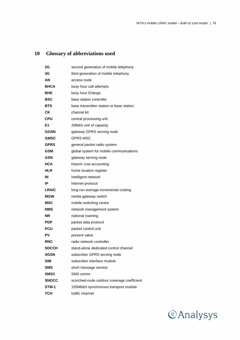
NITA s mobile LRAIC model
draft v2 cost model | 76
10 Glossary of abbreviations used
2G second generation of mobile telephony
3G third generation of mobile telephony
AN access node
BHCA busy hour call attempts
BHE busy hour Erlangs
BSC base station controller
BTS base transmitter station or base station
CK channel kit
CPU central processing unit
E1 2Mbit/s unit of capacity
GGSN gateway GPRS serving node
GMSC GPRS MSC
GPRS general packet radio system
GSM global system for mobile communications
GSN gateway serving node
HCA historic cost accounting
HLR home location register
IN intelligent network
IP Internet protocol
LRAIC long-run average incremental costing
MGW media gateway switch
MSC mobile switching centre
NMS network management system
NR national roaming
PDP packet data protocol
PCU packet control unit
PV present value
RNC radio network controller
SDCCH stand-alone dedicated control channel
SGSN subscriber GPRS serving node
SIM subscriber interface module
SMS short message service
SMSC SMS centre
SNOCC scorched-node outdoor coverage coefficient
STM-1 155Mbit/s synchronous transport module
TCH traffic channel

NITA s mobile LRAIC model
draft v2 cost model | 77
TRX transceiver unit
TSC transit switch
UMTS universal mobile telecommunications systems
VMS voicemail system
WACC weighted average cost of capital

Annex A: Draft v2 cost model for TDC
See separate file

Annex B: Draft v2 cost model for Sonofon
See separate file

Annex C: Draft v2 cost model for Telia
See separate file

Annex D: Draft v2 cost model for Hi3G
See separate file

Annex E: Cost of capital
As described in the conceptual approach to the LRAIC model development, the CAPM and
WACC methods are used for the calculation of the cost of capital for the mobile operators.
The cost of capital is to be calculated under two different situations:
the cost of capital for an efficient supplier of mobile services in Denmark
the cost of capital for each actual operator in Denmark
reflecting any differing
characteristics from the first calculation.
In this annex, the parameters used in the calculation of the WACC are described.
E.1 Calculation
The cost model will require a cost of capital (WACC) to be specified. Pre-tax weighted
average cost of capital is calculated as follows:
ED
EC
ED
DCWACC ed
Where:
dC is the cost of debt
eC is the pre-tax cost of equity
D
is the value of the operator s debt
E
is the value of the operator s equity
Since these parameters, or estimates of them, are most readily available in nominal form,
we calculate the nominal pre-tax WACC and convert it to real1 pre-tax WACC, as follows:
)1(
tax -pre Nominaltax -pre Real
CPI
WACCWACC
1 We have found it more transparent to construct real-terms bottom-up mobile LRIC models. Either method requires a CPI to be
specified (either within the price trends, or the WACC).

NITA s mobile LRAIC model
draft v2 cost model | 3
In the calculation shown above, CPI is the rate of inflation as measured by the Consumer
Price Index.
In the following sub-sections we discuss the assumptions behind each of the parameters in
this calculation.
E.1.1 Cost of debt
)()1( Dfd RRTC
is the cost of debt, where Rf is the risk-free rate, RD is the
company s debt premium and T is the corporate tax rate.
The corporate tax rate is the rate that is applicable to the forward-looking business of the
mobile operators in Denmark. The debt premium that must be offered by a company
specifies the rate above the risk-free rate which debt providers of the company are offered
in return for debt funding. Typically, the debt premium varies with the gearing of the
company
for a higher proportion of debt funding, a greater debt premium must be
offered. This higher premium accounts for the greater financial risk borne by debt
providers and the requirement to fund interest payments out of cashflows.
E.1.2 Cost of equity
We calculate the cost of equity using the capital asset pricing model (CAPM) as follows:
efe RRC
Where:
fR is risk-free rate of return
eR is the equity risk premium
is a measure of how risky a particular company or sector is relative to the national
economy as a whole.
Each of these parameters is now discussed in turn.

NITA s mobile LRAIC model
draft v2 cost model | 4
Risk-free rate of return, fR
The risk-free rate of return is usually taken as that of a long-term government bond. In
NITA s prior work on WACC, a ten-year government bond has been used.
Equity risk premium, eR
Equity risk premium is the increase over the risk-free rate of return that investors demand
from equity. Usually, companies listed on the national stock market are taken as the sample
over which this average is calculated.
Beta for mobile operators,
An accurate empirical determination of requires very large amounts of historical data. It
is therefore an area of considerable subjectivity. Only in the US, and perhaps in a few other
countries with very large stock markets and long histories, have estimates of
been
practicable.
However, given that
represents the risk of a particular industry or company relative to
the market as a whole, one would expect the
of a particular type of company
in this
case a mobile phone company
to be similar across different countries. Comparing
in
this manner requires an un-levered (asset) rather than a levered (equity) :
asset = equity / (1+D/E)
The ERG report on WACC2 provides a European selection of asset ranging from 0.80 to
1.39.
2 http://www.erg.eu.int/doc/publications/erg_07_05_pib_s_on_wacc.pdf
NITA s mobile LRAIC model
draft v2 cost model | 5
E.1.3 Debt/equity (D/E) ratio
Finally, it is necessary to define a funding structure for the market player, based upon an
estimate of the (optimal) proportion of debt and equity in the business. NITA aims to
establish a target gearing for this part of the calculation.
E.2 Sensitivity of the cost of capital to varying the input parameters
In constructing a WACC calculation it is necessary to specify the gearing of the company
(its proportion of debt compared to equity funding) in order to weight the relative costs of
debt and equity. The gearing of the company then also influences the calculation of the
equity, which specifies the rate return required on the equity side, and the debt premium,
which specifies the rate of return on the debt side. Equity returns are provided post-tax and
debt returns are provided pre-tax, therefore in calculating the pre-tax weighted average cost
of capital of a typical mobile operator it can be shown that the cost of capital is broadly
insensitive to the gearing input:
With a higher gearing, a greater proportion of the cost of capital is due to debt
returns at a lower rate than equity returns. However, with a higher gearing the debt
premium and equity also increases. These increases broadly counteract the benefit
of sourcing a greater proportion of funding from (lower cost) debt, and this is
otherwise known as the Miller-Modiglani hypothesis.
As such, the level of the cost of capital is most strongly affected by the input of asset.
E.3 Application to Denmark
Risk-free rate of return, fR
The effective interest rate on a government bond with duration of ten years has been used
as an estimate for the forward-looking nominal risk-free interest. The effective interest rate
for the bond will be estimated as the average of the last 24 months. The current estimation

NITA s mobile LRAIC model
draft v2 cost model | 6
is however based on an average of 12 month average nominal rate of return for a ten-year
government bond for the period November 2006 to October 2007 of 4.20%.3
Equity risk premium, eR
As it is more risky to invest in stocks (equity) than invest in the risk-free government
bonds, investors demand a risk premium when investing in stocks. In 2002, NITA used an
equity risk premium of 3.75%.4 This choice was made by evaluating seven different studies
of the Danish risk premium
using forward-looking as well as historical approaches
that
applied arithmetical as well as geometrical averages based on time periods of 50 100
years.
The ERG report on WACC5 shows that European regulators use an equity risk premium
that is between 3.75% and 7.20%. The most recent study6 of investment returns over the
101 years from 1900 2000 shows that the equity risk premium for Denmark is 2.0%
(geometric mean) and 3.3% (arithmetic mean), and for the world it is 4.6% (geometric
mean) and 5.6% (arithmetic mean). Furthermore, the study estimates that the forward-
looking risk premium for the world is 3% (geometric mean) and a little below 4%
(arithmetic mean).
Furthermore, NITA has noted that, in 2005, the Danish Energy Regulatory Authority
(DERA) found it to be true and fair to use a premium of 3.75% as part of the regulation of
the gas transmission and distribution networks.7
3 Source: Statistics Denmark.
4 Source: NITA, Report on the Hybrid Model, August 2002.
5 http://www.erg.eu.int/doc/publications/erg_07_05_pib_s_on_wacc.pdf.
6 Dimson, Marsh and Staunton (2002): Triumph of the optimists: 101 years of investment returns , Princeton University Press,
Princeton, New Jersey and Oxford.
7 DERA s decission from 29 August 2005: Indtægtsrammeregulering af naturgasdistributionsselskaberne fastsættelsen af
forrentningssatser for 2005 samt udmelding af indtægtsrammer for 2005, http://www.energitilsynet.dk/afgoerelser-
mv/4/1/afgoerelser-gas/indtaegtsrammeregulering-af-naturgasdistributi-onsselskaber-godkendelse-af-regulatoriske-aab-
ningsbalancer-pr-1-januar-2005-godkendelse-af-omkostningsrammer-og-godkendelse-af-11-om-kostninger-for-2005/

NITA s mobile LRAIC model
draft v2 cost model | 7
NITA therefore considers it to be appropriate that the equity risk premium should remain at
3.75%.
Tax rate, T
The Danish corporate tax rate of 25% should be applied in the cost of capital calculation.
Gearing, ED
D
The gearing denotes loan capital as a proportion of the total financing needs of a company.
Generally, the demand for return on equity will be higher than the demand for return on
loan capital. An increasing gearing will lead to an increasing debt risk premium as creditors
demand a higher interest rate if there is less certainty in getting repaid.
Therefore, in financial theory it is assumed that an optimal financing structure, that
minimises the cost of capital, actually exists. This is called target gearing. In practice, this
optimal gearing is very difficult to determine and it will vary according to the type and
form of the company.
The debt proportion of mobile companies typically varies from 0% to around 30%. Mobile
operators generally have a lower reliance on debt than fixed operators because of the
greater variability in costs and returns compared with incumbent fixed line operations.
However, as discussed above, the final result is generally insensitive to this input. Often, a
cost of capital is estimated for a range of gearing rates (e.g. NITA s 2002 and 2005 reports
on the fixed network LRAIC modelling; PTS s assessment of the cost of capital for its
mobile LRIC model, 4 July 2004).
Debt premium, DR
The debt premium for a mobile operator increases with the rate of gearing. At 10% gearing,
the debt premium is approximately 1 2%. The debt premium increases to around 2 3% at a

NITA s mobile LRAIC model
draft v2 cost model | 8
gearing of 30%. These premium rates are consistent with NITA s previous cost of capital
determinations in the fixed network. In fixed networks, where costs are less variable, debt
funding generally represents a higher proportion with debt premiums for a given gearing.
They are 1 2% lower than in the mobile situation, where costs are generally more variable.
Asset beta, asset
When an agent invests in any given stock, two types of risks are assumed to exist
a
systematic and an unsystematic risk. The unsystematic risk is caused by the risk connected
to the specific stock. The investor may avoid this risk by spreading (diversifying) the
investment on a number of different assets. Obviously, a collection of assets (a portfolio)
will always exist, eliminating the unsystematic risk.
The systematic risk, related to the investment, is due to the fact that it is generally risky to
invest in the stock market. This risk is denoted by
and is measured as the covariance
between the return of the specific stock and the return of the market portfolio in relation to
the variance of the return on the market portfolio. For the investor, it is not possible to
avoid the systematic risk, which is why a risk premium will be demanded. The magnitude
of this will vary with the covariance of the specific stock and the overall market
fluctuations.
It is possible to estimate asset through a comparison of the fluctuations in a company s
stock relative to a broad market portfolio over a number of years. However, such
measurements will always be uncertain and will produce a wide range of values depending
on the methodology. Again, under such circumstances, regulators often have to estimate
the cost of capital for a broad range of asset values.
However, by reviewing the range of measurements carried out by third parties, it is
possible to provide some consistency to this range. Indeed, as noted above, the ERG
provides its own range to this relevant parameter. We find the following conclusions for
the reasonable range of asset:

NITA s mobile LRAIC model
draft v2 cost model | 9
0.8 1.0 for integrated Scandinavian fixed and mobile telecoms providers such as TDC,
Telenor or TeliaSonera, which may be disaggregated into separate
asset for the fixed
and mobile parts.
0.8 1.6 for mobile operators, depending on their degree of investment risk.8
Therefore, NITA estimates that the
asset applicable to the funding of the mobile operators
in Denmark varies quite widely, ranging from 0.9 1.5 depending on the operator.
E.4 Results
NITA considers that the cost of capital is generally insensitive to the debt proportion
applied to the weighting calculation, though it is likely that the Danish mobile operators
fall into two types of company from a funding risk perspective. Based on this NITA
considers the differences between these two groups to be uncertain and therefore finds it
most appropriate to choose a beta value of 1.1 for all companies. The WACCs calculated
with 0% gearing and an un-geared asset beta are as follows:
<--Range for TDC, Sonofon, Telia --->
<---------- Range for Hi3G ----------->
Efficient
operator
Low Beta Lower mid
Beta
High mid
Beta
High Beta
Risk-free rate, nominal 4.20% 4.20% 4.20% 4.20% 4.20%
Equity risk premium 3.75% 3.75% 3.75% 3.75% 3.75%
Asset beta 0.9 1.0 1.2 1.5 1.1
Tax rate 25% 25% 25% 25% 25%
Pre-tax cost of equity, nominal 10.1% 10.6% 11.6% 13.1% 11.1%
Inflation9 2.2% 2.2% 2.2% 2.2% 2.2%
Pre-tax cost of capital, real 7.7% 8.2% 9.2% 10.7% 8.7%
Exhibit E.1: Cost of capital [Source: Analysys]
8 Investment risk is characterised by the degree of operator maturity, market share, date of entry and technology prospects.
9 Average of inflation for the next ten years, Source: EIU.

NITA s mobile LRAIC model
draft v2 cost model | 10
For comparison, the WACC calculated at a 10% gearing with a 2% debt premium, and the
WACC at a 30% gearing with a 2.5% debt premium, are also shown below. As can be
seen, the level of WACC is not materially affected by the debt assumptions.
Pre-tax cost of capital, real Low Beta Lower mid
Beta
High mid
Beta
High Beta Efficient
operator
0% debt, 100% equity, 7.7% 8.2% 9.2% 10.7% 8.7%
10% debt, 2% debt premium 7.7% 8.2% 9.1% 10.5% 8.6%
30% debt, 2.5% debt premium 7.7% 8.2% 9.1% 10.4% 8.6%
Exhibit E.2: Effect of debt assumptions [Source: Analysys]

Annex F: Model updates
This annex summarises the updates made to the model in producing the draft v2 cost
model. The table added to the model files (sheet: Change Summary) lists the specific
application of model updates to each mobile operator.
Updates for draft v1 model Notes
PS data proportion Set to 75% based on NITA information
Soft-handover allowance Set to 30% based on Analysys estimates
Exhibit F.1: Draft v1 model updates [Source: Analysys]

NITA s mobile LRAIC model
draft v2 cost model | 12
Updates for draft v2 model Notes
Deployment of MMSC Commences with packet data services
Deployment of content platform Commences with packet data services
Routeing factor for 3G interconnect infrastructure Routeing factor added for national roaming incoming traffic
Inputs and calculations for Tele2 and Barablu Model expanded to accommodate MVNOs
Calculation of "BHCA per minute" for use in the cost allocation matrix
Calculation adjusted to be based on 2007 demand parameters because when based on 2006 services, some zeros for non-launched 3G services flow through to give zero cost allocation to 3G services
New services added to complete the set of national roaming services for 3G
Model expanded to accommodate more services, though not all operators utilise/carry 3G national roaming
Added calculation of book value of fully depreciated assets
Only used for one operator's reconciliation
BTS, BSC and MSC utilisation input changed to a time series
To improve calibration aspects of historic evolution
Reconciliation files created for each operator To show reconciliation comparisons
Categorisation of capital and operating expenditures for each operator
Operator-specific categorisation of costs set up to assist in reconciliation comparisons
Ringing time added to the radio routeing factors of each voice conveyance service
In response to operator comments
Various changes to data inputs as listed in hearing note
Various see hearing notes
Signalling channels per TRX Extended to be operator-specific input
Maximum utilisation of a BTS Revised algorithm so that maximum utilisation applies to the physical capacity of the BTS, rather than both the physical and spectral capacity. This is because the reasons for under-utilising the capacity of BTSs on average relate to the physical domain (i.e. to cause deployment of more sites for "quality") rather than the specific constraint which may arise in the situation of (very) limited spectrum
Erlang table functions Revised formula to look one row further (see TDC hearing response)
Cell breathing quadratic approximation added See Public Annex D
Price trend inputs populated from operator information and estimates
Same underlying trends applied to all operators
Unit equipment prices added Operator-specific inputs based on bottom-up unit prices and top-down reconciliation
A matrix of 0s and 1s has been applied to the unit cost result matrices
To not show unit costs when services do not exist
Revised TSC series of MSC look-up table To improve TSC calibration
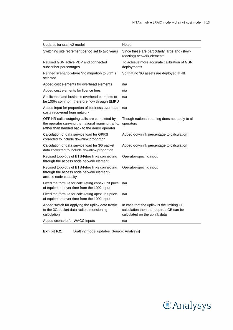
NITA s mobile LRAIC model
draft v2 cost model | 13
Updates for draft v2 model Notes
Switching site retirement period set to two years Since these are particularly large and (slow-reacting) network elements
Revised GSN active PDP and connected subscriber percentages
To achieve more accurate calibration of GSN deployments
Refined scenario where "no migration to 3G" is selected
So that no 3G assets are deployed at all
Added cost elements for overhead elements n/a
Added cost elements for licence fees n/a
Set licence and business overhead elements to be 100% common, therefore flow through EMPU
n/a
Added input for proportion of business overhead costs recovered from network
n/a
OFF NR calls: outgoing calls are completed by the operator carrying the national roaming traffic, rather than handed back to the donor operator
Though national roaming does not apply to all operators
Calculation of data service load for GPRS corrected to include downlink proportion
Added downlink percentage to calculation
Calculation of data service load for 3G packet data corrected to include downlink proportion
Added downlink percentage to calculation
Revised topology of BTS-Fibre links connecting through the access node network element
Operator-specific input
Revised topology of BTS-Fibre links connecting through the access node network element-access node capacity
Operator-specific input
Fixed the formula for calculating capex unit price of equipment over time from the 1992 input
n/a
Fixed the formula for calculating opex unit price of equipment over time from the 1992 input
n/a
Added switch for applying the uplink data traffic to the 3G packet data radio dimensioning calculation
In case that the uplink is the limiting CE calculation then the required CE can be calculated on the uplink data
Added scenario for WACC inputs n/a
Exhibit F.2: Draft v2 model updates [Source: Analysys]